Convergence map with action-angle variables based on square matrix for nonlinear lattice optimization

Abstract

To analyze nonlinear dynamic systems, we developed a new technique based on the square matrix method. We propose this technique called the “convergence map” for generating particle stability diagrams similar to the frequency maps widely used in accelerator physics to estimate dynamic aperture. The convergence map provides similar information as the frequency map but in a much shorter computing time. The dynamic equation can be rewritten in terms of action-angle variables provided by the square matrix derived from the accelerator lattice. The convergence map is obtained by solving the exact nonlinear equation iteratively by the perturbation method using Fourier transform and studying convergence. When the iteration is convergent, the solution is expressed as a quasi-periodic analytical function as a highly accurate approximation, and hence the motion is stable. The border of stable motion determines the dynamical aperture. As an example, we applied the new method to the nonlinear optimization of the NSLS-II storage ring and demonstrated a dynamic aperture comparable to or larger than the nominal one obtained by particle tracking. The computation speed of the convergence map is 30 to 300 times faster than the speed of the particle tracking, depending on the size of the ring lattice (number of superperiods). The computation speed ratio is larger for complex lattices with low symmetry, such as particle colliders.

I Introduction

The field of nonlinear dynamics has a very wide area of application in science Lichtenberg and Lieberman (1992). One of the topical applications is to study the question of the long-term behavior of charged particles in storage rings. One would like to analyze particle behavior under many iterations of the one-turn map. The most accurate and reliable numerical approach is particle tracking in a magnet lattice model with appropriate integration methods. This approach is implemented in many computer codes. However, particle tracking is computing resource-intensive, so parallel codes and long computation time are often required. For fast analysis, however, one would like a more compact representation of the one-turn map out of which to extract relevant information. Among the many approaches to this issue, we may mention canonical perturbation theory, Lie operators, power series, normal form Lichtenberg and Lieberman (1992); Ruth (1987); Guignard (1978); Schoch (1958); Dragt (1988); Berz (1989); Chao (2002); Bazzani et al. (1994); Forest (1998); Forest et al. (1989); Michelotti and Lifshitz (1995) , etc. The results are often expressed as polynomials. However, for increased perturbation, near resonance, or for large oscillation amplitudes, these perturbative approaches often have insufficient precision. The stability analysis of the beam trajectory and calculation of the dynamic aperture requires an accurate solution of the nonlinear dynamical equation. Hence there is a need to extract the information about long-term particle behavior from the one-turn map based on these polynomials with high precision and high speed.

The square matrix analysis Yu and Nash ; Yu (2017); Yu et al. ; Hao et al. has a good potential to explore this area. In this paper, we introduce a “convergence map” calculated using action-angle variables in the form of polynomials provided by a square matrix, which is derived from the one-turn map for an accelerator lattice. Since the iterations leading to the solution of the nonlinear dynamic equations expressed by these action-angle variables can be carried out by Fourier transform, the computation speed is very high, the details are presented in Section II. Using the NSLS-II lattice Dierker (2007) as an example, we show the nonlinear lattice optimization using the convergence map results in a dynamic aperture comparable to or larger than that obtained by particle tracking but the calculations are much faster. In comparison with the frequency map Nadolski and Laskar (2003) calculated by particle tracking, the convergence map is different, even though it provides nearly the same information about the stable region of the motion but the computation time is shorter by a factor of 30 to 300 depending on the size and order of symmetry of the ring lattice (number of superperiods). The computation speed ratio is larger for complex lattices with low symmetry, such as particle colliders.

As an example, Figure 1 shows a comparison of the convergence map (a) and the frequency map from tracking (b) calculated with the same number of points in the horizontal (x) and vertical (y) plane for the nominal lattice of NSLS-II (1 superperiod). The computation speed ratio is about 30 for this case. Figure 2 represents the computation time of the convergence map and the frequency map as a function of the number of points in both planes for one superperiod and the whole NSLS-II ring consisting of 15 superperiods.

One point we found is that the convergence map is more time-efficient because the lattice model is represented by truncated power series (TPS) Berz (1989); PyT and this time-consuming calculation is done only once before the map generation, unlike the frequency map which requires the tracking through the full lattice for every point on the map.The details will be explained in the following sections.

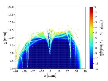
Figure 1: The convergence map (left figure) and the frequency map (right figure) for NSLS-II bare lattice.

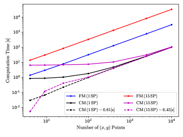
Figure 2: Computation time comparison between convergence map (CM) and frequency map (FM) analyses with different numbers of initial transverse coordinate points and with one super-period (SP) and the whole ring (15 SPs) of NSLS-II. The dash lines correspond to the computation times without the initial setup times (mainly TPSA calculations).

In Section II.A, we first introduce the square matrix equation for nonlinear dynamics, using the Henon map Wayne (1990); Hao et al. as an example. Then, in Section II.B, we show that a set of polynomials derived from the left eigenvectors in the Jordan decomposition of the square matrix can be used as a set of approximate action-angle variables, i.e. the trajectory represented by these variables follow a circle with a small deviation from a rotation with a constant rotation speed.

In Section III, we show that a suitable linear combination of these action-angle variables can be used to minimize the deviation from a pure rotation (i.e., a deviation from an exact action-angle variable). Then, considering the small deviation as a perturbation, we show it is possible to write an exact equation for the action-angle variables with the deviation as a perturbation term. We develop a method to solve this perturbation equation of motion using Fourier transform. That is, we develop an iteration procedure to generate a sequence of new action-angle variables to improve their precision, so in each iteration step the new solution has not only less deviation from a pure rotation, it is also closer to the exact solution of the equation. In short, we use an analytical periodic function to approximate the exact solution. When the iteration process is convergent the sequence approaches the exact solution.

In Section IV, we test the precision numerically using the convergence of the sequence as a criterion for the deviation of the solution from a pure rotation. Actually, the convergence criterion can be used to clarify the meaning of a “small” deviation from a pure rotation: if the deviation is “small”, the sequence should be convergent. Applying the convergence criterion in the x,y plane leads to a “convergence map” , which is entirely different from the frequency map Nadolski and Laskar (2003), but carries similar information about the trajectory, amplitude-tune dependence, stability of the trajectory and the dynamic aperture.

In Section V, we describe the convergence map application to nonlinear lattice optimization using NSLS-II as an example, in comparison with particle tracking.

In Section VI, we show the convergence map is much faster than tracking for the same number of points taken for the phase space. Hence the convergence map can be used as an efficient tool for the nonlinear optimization of storage ring lattices.

Then in Section VII, we compare the particle survival turn numbers in tracking with the number of points taken for the action-angle variables in a period of the trajectory before the iteration procedure diverges. Our numerical study indicates their similar relation to dynamic aperture. This is the reason why the convergence map can be used to study the dynamic aperture.

Section VIII is the conclusion.

II Square matrix

II.1 Square matrix equation for nonlinear dynamics

We consider the equations of motion of a nonlinear dynamic system with periodic structure such as Hills equation, it can be expressed by a square matrix.

If we use the complex Courant-Snyder variable $z=x-ip$, its conjugate and powers $z,z^{\ast},z^{2},...$ as a column vector $Z$, the one turn map can be represented by a large square matrix $M$ using

$$Z=MZ_{0}$$ (1)

The column vector $Z_{0}$ represents the initial value of the column vector $Z$ before the one turn mapping.

For an example of Hénon map Wayne (1990),

$$\begin{split}x&=x_{0}\cos\mu+p_{0}\sin\mu+\epsilon x_{0}^{2}\sin\mu\\ p&=-x_{0}\sin\mu+p_{0}\cos\mu+\epsilon x_{0}^{2}\cos\mu\end{split},$$ (2)

we use a variable transformation $z=x-ip$ , $z^{\ast}=x+ip$ ,$z_{0}=x_{0}-ip_{0}$ and $z_{0}^{\ast}=x_{0}+ip_{0}$ to rewrite this equation into a form of the first two rows of the following equation Eq.(3). Then, using these firt two rows, $z,z^{\ast}$ and their higher power monomials after one turn of rotation, or after one element in an accelerator lattice, can be written as a truncated power series expansion of the initial $z_{0}=x_{0}-ip_{0}$ and $z_{0}^{\ast}=x_{0}+ip_{0}$. For example, up to 3rd order, we have:

$$\begin{split}z&=e^{i\mu}z_{0}-\frac{i}{4}\epsilon e^{i\mu}z_{0}^{2}-\frac{i}{2}\epsilon e^{i\mu}z_{0}z_{0}^{\ast}-\frac{i}{4}\epsilon e^{i\mu}z_{0}^{\ast 2}\\ z^{\ast}&=e^{-i\mu}z_{0}^{\ast}+\frac{i}{4}\epsilon e^{-i\mu}z_{0}^{2}+\frac{i}{2}\epsilon e^{-i\mu}z_{0}z_{0}^{\ast}+\frac{i}{4}\epsilon e^{-i\mu}z_{0}^{\ast 2}\\ z^{2}&=e^{2i\mu}z_{0}^{2}-\frac{i}{2}\epsilon e^{2i\mu}z_{0}^{3}-i\epsilon e^{2i\mu}z_{0}^{2}z_{0}^{\ast}-\frac{i}{2}\epsilon e^{2i\mu}z_{0}z_{0}^{\ast 2}\\ zz^{\ast}&=z_{0}z_{0}^{\ast}+\frac{i}{4}\epsilon z_{0}^{3}+\frac{i}{4}\epsilon z_{0}^{2}z_{0}^{\ast}-\frac{i}{4}\epsilon z_{0}z_{0}^{\ast 2}-\frac{i}{4}\epsilon z_{0}^{\ast 3}\\ z^{\ast 2}&=e^{-2i\mu}z_{0}^{\ast 2}+\frac{i\epsilon}{2}e^{-2i\mu}z_{0}^{2}z_{0}^{\ast}+i\epsilon e^{-2i\mu}z_{0}z_{0}^{\ast 2}+\frac{i\epsilon}{2}e^{-2i\mu}z_{0}^{\ast 3}\\ z^{3}&=e^{3i\mu}z_{0}^{3}\\ ...&\\ z^{\ast 3}&=e^{-3i\mu}z_{0}^{\ast 3}\end{split},\text{ with \hskip 10.03749pt}Z\equiv\left(\begin{array}[]{c}z\\ z^{\ast}\\ z^{2}\\ zz^{\ast}\\ z^{\ast 2}\\ z^{3}\\ \vdots\\ z^{\ast 3}\end{array}\right)$$ (3)

Because in this equation the monomial term of power order $m$ at the left hand side only have power terms of initial monomial terms with power order higher than $m$ at the right hand side, the coefficients in Eq.(3) form an upper-triangular $10\times 10$ square matrix $M,$ such that Eq.(3) can be written as $Z=MZ_{0}$. In general, there are constant terms in the expansion. In this example, the offset of x is zero, so the constant terms are also zeros. The vector $Z$ spans a 10 dimensional linear space. The matrix $M$, when operated on $Z_{0}$ , represents a rotation of $Z$ in this space. We remark here that even though we mostly use $M$ to represent one turn map for a storage ring, each element in the storage ring dynamics or other nonlinear dynamics problem can also be written as a square matrix, then $M$ would be a product of the square matrix of the elements.

II.2 Eigenvectors of Jordan blocks of square matrix $M$ as Approximate Action-Angle Variables

All square matrices can be transformed into Jordan form Kågström and Ruhe (1980, 1980), this transform is particularly very simple for a triangular square matrix. A detailed description is given, e.g., in Ref Yu (2017); Kågström and Ruhe (1980, 1980). For any given square matrix $M$, there are well known methods to calculate an eigenvalue $\mu$, a transformation matrix $U$ and a Jordan matrix $\tau$ so that every row of the matrix $U$ is a (generalized) left eigenvector of $M$, with the i${}^{\text{th}}$ row of $U$ denoted by $u_{i}$ satisfying

$$\begin{split}UM=e^{i\mu I+{\tau}}U\end{split}$$ (4)

As an example, for the case of the Henon map in Eq.2 and Eq. 3 with tune $\mu$ , one of the eigenvalues of $M$ is $e^{i\mu}$, the Jordan matrix $\tau$ has the form

$$\tau=\begin{bmatrix}0&1\\ 0&0\end{bmatrix}$$ (5)

, with $I$ as the identity matrix. The Matrix U can be found as

$$U=\left(\begin{array}[]{c}u_{0}\\ u_{1}\end{array}\right)=\left({\scriptscriptstyle\begin{array}[]{cccccccccc}0&1&0&\frac{i}{4\left(-1+e^{i\mu}\right)}&\frac{ie^{i\mu}}{2-2e^{i\mu}}&\frac{ie^{3i\mu}}{4-4e^{3i\mu}}&-\frac{1}{8\left(-1+e^{i\mu}\right)^{2}}&0&U_{0,8}&U_{0,9}\\ 0&0&0&0&0&0&0&U_{1,7}&0&0\end{array}}\right)$$ (10)

with

$$U_{0,8} =\frac{e^{2i\mu}-e^{3i\mu}+e^{4i\mu}}{-8e^{i\mu}-8e^{3i\mu}+8e^{4i\mu}+8}$$

$$U_{0,9} =-\frac{e^{5i\mu}}{8\left(-1+e^{i\mu}\right)^{2}\left(1+e^{2i\mu}\right)\left(e^{i\mu}+e^{2i\mu}+1\right)}$$

$$U_{1,7} =\frac{e^{i\mu}\left(3e^{i\mu}+3e^{2i\mu}+2e^{3i\mu}+2\right)}{8\left(-1+e^{3i\mu}\right)}$$

In the general case, the Jordan matrix $\tau$ always has much lower dimension than the mapping matrix $M$, and has the form

$$\tau=\begin{bmatrix}0&1&0&...&0\\ 0&0&1&...&0\\ 0&0&...&...&0\\ 0&0&0&...&1\\ 0&0&0&...&0\end{bmatrix}.$$ (11)

In the example for the case of 4 variables $x,p_{x},y,p_{y}$ at $3^{\text{rd}}$ order, as for the storage ring lattice example to be used later, the matrix $M$ is a $35\times 35$ matrix, Jordan matrix $\tau$ is exactly same as the form of Eq.5, the matrices $U_{x}$ and $U_{y}$ are $2\times 35$ transformation matrix, for eigenvalues $\mu_{x}$ and $\mu_{y}$ respectively. For the convergence map study in our example, high precision is achieved without using power order higher than 3, and when it is convergent the result approaches the solution precisely.

As $Z=MZ_{0}$, Eq.(4) gives

$$UZ=UMZ_{0}=e^{i\mu I+{\tau}}UZ_{0}.$$ (12)

Therefore a transformation is defined as

$$\begin{split}W&\equiv UZ\\ W_{0}&\equiv UZ_{0}\end{split}$$ (13)

$W$ represents the projection of the vector $Z$ onto the invariant subspace spanned by the left eigenvectors $u_{j}$ given by the rows of the matrix $U$, such that each row of $W$ is $w_{j}=u_{j}Z$, a polynomial of $z,z^{\ast}$. Then Eq.(12) implies the operation of one turn map $Z=MZ_{0}$, corresponds to a rotation in the invariant subspace represented by

$$W=e^{i\mu I+{\tau}}W_{0}.$$ (14)

As an example, for the Henon map Eq.(2,3), because $U$ and $Z$ are given by Eq.(10, 3) we have:

$$w_{0} =u_{0}Z= z+\frac{i}{4\left(-1+e^{i\mu}\right)}z^{2}+\frac{ie^{i\mu}}{2-2e^{i\mu}}zz^{\ast}+\frac{ie^{3i\mu}}{4-4e^{3i\mu}}z^{\ast 2}$$

$$-\frac{1}{8\left(-1+e^{i\mu}\right)^{2}}z^{3}+\frac{e^{2i\mu}-e^{3i\mu}+e^{4i\mu}}{-8e^{i\mu}-8e^{3i\mu}+8e^{4i\mu}+8}zz^{\ast 2}$$

$$-\frac{e^{5i\mu}}{8\left(-1+e^{i\mu}\right)^{2}\left(1+e^{2i\mu}\right)\left(e^{i\mu}+e^{2i\mu}+1\right)}z^{\ast 3}$$

$$w_{1} =u_{1}Z= \frac{e^{i\mu}\left(3e^{i\mu}+3e^{2i\mu}+2e^{3i\mu}+2\right)}{8\left(-1+e^{3i\mu}\right)}z^{2}z^{\ast}$$

The lowest power order term of $w_{0}$ is the linear term $z$, compared with 3rd power order term $z^{2}z^{\ast}$ for $w_{1}$.

In general, for small amplitude the lowest order terms in $W$ dominate. Since $W$ rotates in the invariant subspace of $Z$, for sufficiently small amplitude, when the higher power term (for example in Hénon example, Eq.(3)) is negligibly small, the equation is nearly linear, hence the absolute value of each row $|w_{j}|=|u_{j}Z|$ of $W$ is approximately invariant with a phase advance given by $\mu+\phi$, where $\mu$ is the linear tune, and $\phi\ll\mu$ is the amplitude dependent tune shift. This is related to the KAM theory in nonlinear dynamics.

KAM theory states that the invariant tori are stable under small perturbation (See, for example, Ref Lichtenberg and Lieberman (1992); Broer (2004); Arnold (2009)). In our examples, for sufficiently small amplitude of oscillation in $z$, the invariant tori are deformed and survive, i.e., the motion is quasiperiodic. So the system has a nearly stable frequency, and when the amplitude is small, the fluctuation of the frequency is also small. Since during the dynamical process $W$ remains in the eigenspace of the column space $Z$, after $n$ turns, approximately, the vector $W$ only changes by a phase factor $e^{in(\mu+\phi)}$, i.e.,

$$W=e^{n(i\mu I+{\tau})}W_{0}\cong e^{in(\mu+\phi)}W_{0}.$$ (15)

From a comparison of both sides of Eq.(15) we have,

$$\tau W_{0}\cong i\phi W_{0}.$$ (16)

and $\phi$ is the amplitude dependent tune shift. In Eq.(16) we use the approximate equal sign because for a matrix $\tau$ of finite dimension m, the relation is only an approximation for sufficiently small amplitude. We write the Eq. (15) explicitly using the property of the Jordan matrix $\tau$ given by Eq. (11) as a raising operator:

$$\tau\begin{bmatrix}w_{0}\\ w_{1}\\ ...\\ w_{m-1}\end{bmatrix}=\begin{bmatrix}w_{1}\\ w_{2}\\ ...\\ 0\end{bmatrix}\cong\begin{bmatrix}i\phi w_{0}\\ i\phi w_{1}\\ ...\\ i\phi w_{m-1}\end{bmatrix}$$ (17)

where $w_{j}$’s are the rows of $W_{0}$. Compare the two sides we find

$$i\phi=\frac{w_{1}}{w_{0}}\cong\frac{w_{2}}{w_{1}}\cong\frac{w_{3}}{w_{2}}\dots$$ (18)

In the study of truncated power series, m is finite, hence Eq. (18) is an approximation. The polynomials $w_{m-2},w_{m-1}$ have only high order terms, and as $m$ increases, when the amplitude of $z$ is sufficiently small, the last term in Eq. (18) becomes the ratio of two negligibly small numbers, and is less accurate. Actually the last row of Eq. (17) is impossible, so it can only be taken as an approximation representing the fact that $|\phi w_{m-1}|$ is neglegibly small. In addition to the condition Eq. (18) for a stable motion, obviously, for the amplitude to be nearly constant, another condition is

$$\text{Im}(\phi)\cong 0.$$ (19)

Fig.3 compare the tracking (direct iteration of Eq.(2), red) and $\nu=(\mu+\phi)/2\pi$ (green), with $i\phi=\frac{w_{1}}{w_{0}}$ of Eq.(18). It is clear that $w_{0}$ can be used as an aproximate action-angle variable, even near the resonances $x\sim(0.53,0.68)$.

Figure 3: Compare tune $\nu$ vs.$x$ calculated by tracking with square matrix

In our study of storage ring lattice using its matrix $M$, Eqs.(18) and (19) are confirmed by many numerical examples.

The Eq.(15), derived for $x,y$ planes separately, leads to a set of polynomials $w_{x0},w_{x1},\cdots$, and $w_{y0},w_{y1},\cdots$. Our tracking results confirmed that these polynomials, or linear combinations can be used as a set of approximate action-angle variables: after $n$ turns they are multiplied by a factor of form $e^{in(\mu+\phi)}$ approximately, ie. the trajectory represented by these variabes follow a circle with small deviation from a rotation with uniform rotation speed. In addition, we find that near the stability border the deviation of these actions from constancy provides a measure of the destruction of invariant tori, or a measure of the stability of trajectories and tunes. In the next section, we shall seek for a variable transformation from $x,p_{x},y,p_{y}$ to these action-angle variables such that the nonlinear dynamical equation is transformed into a form which can be solved by an iteration method .

III Perturbation based on action-angle approximation and iteration

In this section, we will detail the iteration method to find the action-angle approximation and its application in predicting particle’s long term stability.

III.1 Variable transform of dynamical quation and perturbation solution

In the previous section, a transformation $U$ is generated by the square matrix method for nonlinear map $M$ to create the new set of variables $w$, so that map $U\circ M\circ U^{-1}$ is approximately a rigid rotation and $w$ serve as approximate action-angle variables. Since the new set of variable $w$ is not unique, we use $v_{1}$ and $v_{2}$ to denote the choice of approximate action. The simplest choice is $v_{1}=w_{x0}$ and $v_{2}=w_{y0}$. Further variable transformation can be found to make the map to be an exact rigid rotation map when there is a quasi-periodic solution for the system.

To formulate the perturbation problem, we rewrite the action-angle variables $v_{1},v_{2}$ as

$$\begin{split}&v_{1}(\theta_{1})\equiv e^{i\theta_{1}}\\ &v_{2}(\theta_{2})\equiv e^{i\theta_{2}}\end{split}$$ (20)

where $\theta_{1},\theta_{2}$ are complex numbers which denote oscillations deviate from rigid rotation with unknown frequency $\omega_{1},\omega_{2}$ with small phase fluctuation (the real part of $\theta_{1},\theta_{2}$ ) and amplitude fluctuation (imaginary part of $\theta_{1},\theta_{2}$). We consider the relation between the 4 variables, $\theta_{1},\theta_{2}$ , their complex conjugate $\theta_{1}^{*},\theta_{2}^{*}$, and $x,p_{x},y,p_{y}$ (to be abbreviated as $X$ in the following) as a variable transformation.

We establish one turn map using $\theta_{1},\theta_{2}$ as dynamic variables, i.e, we consider $\theta_{1,k+1},\theta_{2,k+1}$ as function of $\theta_{1k},\theta_{2k}$ (with $k$ the turn number):

$$\begin{split}&\theta_{1,k+1}=\theta_{1,k}-i\ log\frac{v_{1}(\theta_{1,k+1})}{v_{1}(\theta_{1,k})}\equiv\theta_{1,k}+\phi_{1}(\theta_{1,k},\theta_{2,k})\\ &\theta_{2,k+1}=\theta_{2,k}-i\ log\frac{v_{2}(\theta_{2,k+1})}{v_{2}(\theta_{2,k})}\equiv\theta_{2,k}+\phi_{2}(\theta_{1,k},\theta_{2,k})\end{split}$$ (21)

where $\phi_{1}$ and $\phi_{2}$ are functions which can be found from the map without approximations. Now when there are quasi-periodic solutions we can find a transformation from $(\theta_{1},\theta_{2})$ to a rigid rotation variable pair $(\alpha_{1},\alpha_{2})$, which satisfy

$$\begin{split}&\alpha_{1,k+1}=\alpha_{1,k}+\omega_{1}\\ &\alpha_{2,k+1}=\alpha_{2,k}+\omega_{2}\end{split}$$ (22)

where $\omega_{1}$ and $\omega_{2}$ are the rotation number of the map. By denoting $\Delta\phi_{1,2}\equiv\phi_{1,2}-\omega_{1,2}$, the equations for $(\theta_{1},\theta_{2})$ become

$$\begin{split}&\theta_{1}(\alpha_{1}+\omega_{1},\alpha_{2}+\omega_{2})-\theta_{1}(\alpha_{1},\alpha_{2})=\omega_{1}+\Delta\phi_{1}(\theta_{1}(\alpha_{1},\alpha_{2}),\theta_{2}(\alpha_{1},\alpha_{2}))\\ &\theta_{2}(\alpha_{1}+\omega_{1},\alpha_{2}+\omega_{2})-\theta_{2}(\alpha_{1},\alpha_{2})=\omega_{2}+\Delta\phi_{2}(\theta_{1}(\alpha_{1},\alpha_{2}),\theta_{2}(\alpha_{1},\alpha_{2}))\end{split}$$ (23)

If $v_{1},v_{2}$ are sufficiently close to a pure rotation, then $|\Delta\phi_{1}|,|\Delta\phi_{2}|\ll 1$. The real part of $|\Delta\phi_{1}|,|\Delta\phi_{2}|$ are the phase fluctuation, and their imaginary part is the amplitude fluctuation. This exact equation can be solved by perturbation: initially we take zero order approximation $\theta_{1}^{(0)}=\alpha_{1},\theta_{2}^{(0)}=\alpha_{2}$. Then $X^{(0)}$ is calculated by the inverse function of Eq.(20), and $\Delta\phi_{1}^{(0)},\Delta\phi_{1}^{(0)}$is calculated as given by Eq. (21). When this is substituted to the right hand side of Eq. (23), since $|\Delta\phi_{1}|,|\Delta\phi_{2}|\ll 1$ the error is of second order. Hence to first order the solution satisfies

$$\begin{split}&\theta_{1}^{(1)}(\alpha_{1}+\omega_{1},\alpha_{2}+\omega_{2})-\theta_{1}^{(1)}(\alpha_{1},\alpha_{2})\approx\omega_{1}^{(0)}+\Delta\phi_{1}(\theta_{1}^{(0)}(\alpha_{1},\alpha_{2}),\theta_{2}^{(0)}(\alpha_{1},\alpha_{2}))\\ &\theta_{2}^{(1)}(\alpha_{1}+\omega_{1},\alpha_{2}+\omega_{2})-\theta_{2}^{(1)}(\alpha_{1},\alpha_{2})\approx\omega_{2}^{(0)}+\Delta\phi_{2}(\theta_{1}^{(0)}(\alpha_{1},\alpha_{2}),\theta_{2}^{(0)}(\alpha_{1},\alpha_{2}))\end{split}$$ (24)

where $\omega_{1}^{(1)},\omega_{2}^{(1)}$ are the constant term of the Fourier transform of $\phi_{1}(\alpha_{1},\alpha_{2}),\phi_{2}(\alpha_{1},\alpha_{2})$. This equation can be solved using Fourier transform (see Appendix A about the solution by Fourier transform), the result is the first order approximation $\theta_{1}^{(1)},\theta_{2}^{(1)}$ with frequency $\omega_{1}^{(1)},\omega_{2}^{(1)}$. Then $\theta_{1}^{(1)},\theta_{2}^{(1)}$ is substituted in the right hand side of Eq. (24) to obtain $\theta_{1}^{(2)},\theta_{2}^{(2)}$ as $2^{\text{nd}}$ order approximation.

III.2 Iteration of perturbation solution

This process can be iterated to generate convergent solution to high precision if the amplitude of zero’th order$X^{(0)}$ (obtained from $\theta_{1}^{(0)},\theta_{2}^{(0)}$) is sufficiently close the origin, within the dynamical aperture. At iteration step $k$ (i.e., after k iteration ), the equation is

$$\begin{split}&\theta_{1}^{(k+1)}(\alpha_{1}+\omega_{1},\alpha_{2}+\omega_{2})-\theta_{1}^{(k+1)}(\alpha_{1},\alpha_{2})\approx\omega_{1}^{(k)}+\Delta\phi_{1}^{(k)}(\alpha_{1},\alpha_{2})\\ &\theta_{2}^{(k+1)}(\alpha_{1}+\omega_{1},\alpha_{2}+\omega_{2})-\theta_{2}^{(k+1)}(\alpha_{1},\alpha_{2})\approx\omega_{2}^{(k)}+\Delta\phi_{2}^{(k)}(\alpha_{1},\alpha_{2})\end{split}$$ (25)

where the subscripts denote the iteration number of the corresponding variables. $\omega_{1}^{(k)},\omega_{2}^{(k)}$ are the constant terms of the Fourier transform of $\phi_{1}^{(k)}(\alpha_{1},\alpha_{2}),\phi_{2}^{(k)}(\alpha_{1},\alpha_{2})$. For solution $\theta_{1}^{(k)}(\alpha_{1},\alpha_{2}),\theta_{2}^{(k)}(\alpha_{1},\alpha_{2})$ the corresponding coordinates, denoted as $X^{(k)}$, are calculated as the inverse function of Eq.(20).

The main issue is the convergence of this iteration process. In the neighbourhood of a pure rotation, KAM theory Lichtenberg and Lieberman (1992); Arnold (2009); Broer (2004) proved the existence of analytical solution. In a practical application, instead of trying to prove the existence of exact analytical solution, we apply iteration procedure to find the quasi-periodic solution exploring area with large amplitude or near resonance numerically.

III.3 Minimize deviation from pure rotation by renewing linear combination coefficients within an iteration step

In the numerical tests, we found that keeping the simplest choice, i.e. $v_{1}=w_{x0}$ and $v_{2}=w_{y0}$ does not always yields a successful iteration process for large amplitude particles when numerical simulation suggests a quasi-static orbit exists. As shown in the last section, the polynomials $w_{x0},w_{x1},\cdots$, and $w_{y0},w_{y1},\cdots$ may serve as approximate action angles, therefore we may extend the choice of $v_{1}$and $v_{2}$ to be linear combinations of them to allow the iteration method to start from a better approximation of rigid rotation. The linear combination can be written as:

$$\begin{split}&v_{1}(\theta_{1})\equiv a_{11}w_{x0}(X)+a_{12}w_{x1}(X)+a_{13}w_{y0}(X)+a_{14}w_{y1}(X)\\ &v_{2}(\theta_{2})\equiv a_{21}w_{x0}(X)+a_{22}w_{x1}(X)+a_{23}w_{y0}(X)+a_{24}w_{y1}(X)\end{split}$$ (26)

with $a_{ij}$ as free parameters and $X$ denotes the dynamic variables $(x,p_{x},y,p_{y})$. Here we use the 4 polynomials $w_{x0},w_{x1}$$,w_{y0},w_{y1}$, because our experiences shows for ’convergence map’ we found 4 is often enough to generate the map. In some special cases, for example when we calculate solution for some resonances, more polynomials such as $w_{x2},w_{x3}$$,w_{y2},w_{y3}$ ,obtained from higher order Jordan vectors are used to reach convergence. But the study of solution for resonances is still in progress, hence here we limit our discussion to only 4 polynomials.

In Eq. (24), if the zeroth order approximation, the pure rotation $v_{1}^{(0)}(\theta_{1}^{(0)}(\alpha_{1})),v_{2}^{(0)}(\theta_{2}^{(0)}(\alpha_{2}))$ in Eq. (26), determined by a set of linear combination coefficients $\{a_{i,j}^{(0)}\},(i=1,2),(j=1,2,3,4\}$ (the choice of initial $\{a_{ij}^{(0)}\}$ is discussed in the beginning of Appendix A), are sufficiently close to the solution, then the perturbation $|\Delta\phi_{1}^{(0)}|,|\Delta\phi_{2}^{(0)}|$ in Eq.(24) would be small, the Fourier expansion coefficients except the constant terms ($\alpha_{1},\alpha_{2})$ in the Fourier expansion of $\theta_{1}^{(1)},\theta_{2}^{(1)}$ (see Appendix A) would be small: $|\widetilde{\theta^{(1)}}_{1nm}|\ll 1,\ |\widetilde{\theta^{(1)}}_{2nm}|\ll 1$. The first order solution given by Eq. (24) and the first order approximation $v_{1}^{(0)}(\theta_{1}^{(1)}(\alpha_{1},\alpha_{2})),v_{2}^{(0)}(\theta_{2}^{(1)}(\alpha_{1},\alpha_{2}))$ given by Eq.(26) would provide more accurate solution. In order to enhance the convergence rate we add one step in the iteration, i.e., we use a least square method to minimize the fluctuation term $|\Delta\phi_{1}^{(1)}|,|\Delta\phi_{2}^{(1)}|$ in Eq. (25) by varying the linear combination $\{a_{i,j}\}$ in Eq. (26). The goal of this step is to minimize the deviation from pure rotation of $v_{1}\equiv v_{1}(\theta_{1}^{(1)}(\alpha_{1},\alpha_{2})),$ $v_{2}\equiv v_{2}(\theta_{2}^{(1)}(\alpha_{1},\alpha_{2}))$ using the optimized $\{a_{i,j}^{(1)}\}$ to generate $v_{1}^{(1)}\equiv v_{1}^{(1)}(\theta_{1}^{(1)}(\alpha_{1},\alpha_{2})),$ $v_{2}^{(1)}\equiv v_{2}^{(1)}(\theta_{2}^{(1)}(\alpha_{1},\alpha_{2}))$. This least square method is described in Appendix A.

In addition to this change of the linear combination coefficients $\{a_{i,j}\}$ to make the orbit more close to a pure rotation, another way to speed up the convergence is to further decouple the two sets of points in the trajectory determined by either $\theta_{1}(\alpha_{1},\alpha_{2})$ with fixed $\alpha_{2}$, or by $\theta_{2}(\alpha_{1},\alpha_{2})$ with fixed $\alpha_{1}$. Since the Fourier transform of the trajectory is given by $\widetilde{\theta}_{1nm}$ and $\widetilde{\theta}_{2nm}$ on $n_{\theta}^{2}$ points, as explained in Appendix A, the $\alpha_{1},\alpha_{2}$ phase space is also described by $n_{\theta}^{2}$ points determined by $\alpha_{1i},\alpha_{2j}$, as shown in Fig.5a in the next example section. When the solution is close to a pure rotation, there are two nearly independent functions $\theta_{1}(\alpha_{1},\alpha_{2})\approx\theta_{1}(\alpha_{1})$ and $\theta_{2}(\alpha_{1},\alpha_{2})\approx\theta_{2}(\alpha_{2})$, thus there are two nearly decoupled action-angle variables $v_{1},v_{2}$. In the numerical examples in Section IV Fig.7c,d, we show the trajectory in $v_{1},v_{2}$ planes separately as an example to see how they are nearly decoupled even at the starting point $v_{1}^{(0)},v_{2}^{(0)}$, as is more visible in Fig.7d. The blue dots (for varied $\alpha_{1})$ move aroud each red point with fixed $\alpha_{2}$ forming a small circles. As iteration number increases, the circles reduced their radius to points. This rapid decoupling is clear visible in Fig. 7a,b. The convergence result agree with tracking very well, as will be explained in Fig.6a of the next section. Hence for each fixed $\alpha_{2}$, average $\theta_{2}$ over all $\alpha_{1}$ makes the points more close to the poinst of a pure roation. Same way for each fixed $\alpha_{1}$, we average $\theta_{1}$ over all $\alpha_{2}$. This speeds up the decoupling of $v_{1},v_{2}$, and further speeds up the convergence in our iterations. Thus the averaging process is included as part of the second step.

This step is applied in every iteration $k$: Start from $\{a_{i,j}^{(k)}\}$, $X^{(k)}(\alpha_{1},\alpha_{2})$, obtained in previous iteration, we find $v_{1}^{(k)}(\alpha_{1},\alpha_{2}),v_{2}^{(k)}(\alpha_{1},\alpha_{2})$ and hence $\theta_{1}^{(k)}(\alpha_{1},\alpha_{2}),\theta_{2}^{(k)}(\alpha_{1},\alpha_{2})$ using Eq. (26), then the solution of Eq. (25) gives $\theta_{1}^{(k+1)}(\alpha_{1},\alpha_{2}),\theta_{2}^{(k+1)}(\alpha_{1},\alpha_{2})$. In turn, these lead to $v_{1}^{(k)}(\alpha_{1},\alpha_{2})\equiv v_{1}^{(k)}(\theta_{1}^{(k+1)}(\alpha_{1},\alpha_{2}))$ and $v_{2}^{(k)}(\alpha_{1},\alpha_{2})\equiv v_{2}^{(k)}(\theta_{2}^{(k+1)}(\alpha_{1},\alpha_{2}))$, which can be used to find $X^{(k+1)}$ using the inverse function of Eq. (26). Then the least square method in the Appendix B, followed by the decoupling averaging, is applied to find $\{a_{i,j}^{(k+1)}\}$. Then, $\{a_{i,j}^{(k+1)}\}$ and $X^{(k+1)}$ are the staring point of next iteration. The further optimized $\{a_{ij}^{(k+1)}\}$ in Eq. (26) would correspond to a new set of $v_{1}^{(k+1)}(\alpha_{1},\alpha_{2})\equiv v_{1}^{(k+1)}(\theta_{1}^{(k+1)}(\alpha_{1},\alpha_{2}))$, $v_{2}^{(k+1)}(\alpha_{1},\alpha_{2})\equiv v_{1}^{(k+1)}(\theta_{1}^{(k+1)}(\alpha_{1},\alpha_{2}))$ more close to a pure rotation. The two step cycle of iteration is illustrated in Fig.4.

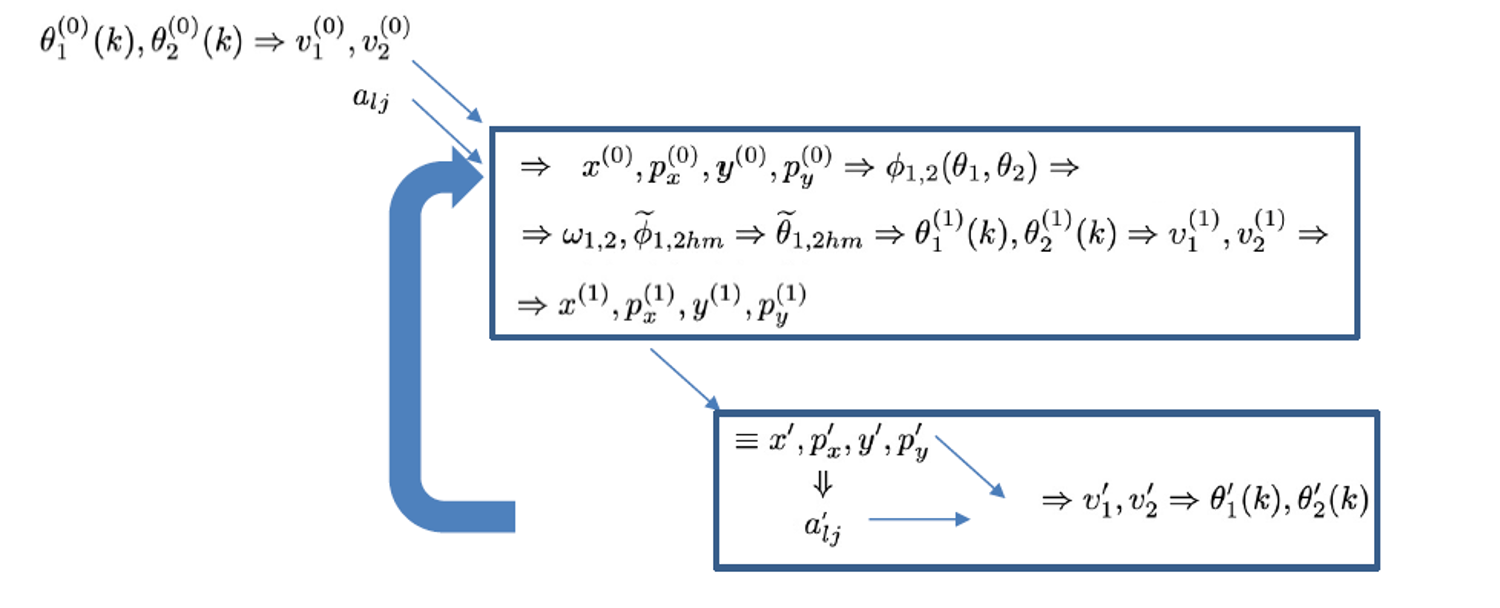
Figure 4: flow diagram for iteration, where $\widetilde{\theta}$, $\widetilde{\phi}$ are the Fourier trasform of $\theta$,$\phi$

There are two steps here in every iteration $k$: 1. find $v_{1}^{(k)},v_{2}^{(k)}$ so it is more close to the exact solution, as the step given by Eq. (25); 2. find new set of linear combination $\{a_{ij}^{(k+1)}\}$ so $v_{1}^{(k+1)},v_{2}^{(k+1)}$ is more close to a pure rotation, as given by Eq. (26) using the least square method in Appendix A.

For each iteration step $k$, $v_{1}^{(k)}(\alpha_{1},\alpha_{2}),v_{2}^{(k)}(\alpha_{1},\alpha_{2})$ and corresponding linear combination $\{a_{ij}^{(k)}\}$ of polynomials $w_{xj},w_{yj}$ give a periodic solution (trajectory) $X^{(k)}(\alpha_{1},\alpha_{2})\equiv x^{(k)}(\alpha_{1},\alpha_{2}),p_{x}^{(k)}(\alpha_{1},\alpha_{2}),y^{(k)}(\alpha_{1},\alpha_{2}),p_{y}^{(k)}(\alpha_{1},\alpha_{2})$. We can use the convergence of $X^{(k)}(\alpha_{1},\alpha_{2})$ as $k$ increases to test the convergence of the iteration based on the Cauchy convergence criterion, i.e., we study $\delta X_{k}$, which is the the standard deviation of $\delta X_{k}\equiv(X^{(k)}(\alpha_{1},\alpha_{2})-X^{(k-1)}(\alpha_{1},\alpha_{2}))_{rms}$, and check whether the sequence of $\delta X_{k}$ decreases exponentially as $k$ increases. If the iteration is convergent, as the iteration $k$ increases, the solution approaches an accurate solution near a limit determined by computer precision. Even though $v_{1}^{(k)},v_{2}^{(k)}$ are approximation to a pure rotation, generally they are not necessarily approaching pure rotation as $k$ increases.

Obviously the iteration method discussed in this section cannot be applied to resonance region where the two action-angle variables becomes correlated, and there is only one independent action-angle variable left. The discussion about resonance case should be addressed in a separate publication rather than this article.

With these provisions, we discuss the numerical application of this iteration steps in the following.

IV Numerical application of convergence map

In practical numerical application, one of the main parameters is the number of indices $m,n={0,1,2,...n_{\theta-1}}$ in Eq. (27). Correspondingly in the inverse Fourier transform of Eq. (27) the variables $\theta_{1},\theta_{2}$ and $\alpha_{1}$,$\alpha_{2}$ also take discrete values at $n_{\theta}^{2}$ points in the $\theta_{1},\theta_{2}$ plane. Fig.5 is an illustration of $\theta_{1}^{(0)}(\alpha),\theta_{2}^{(0)}(\alpha)$ and the result of tracking them one turn.

Figure 5: points in initial $\theta_{1}^{(0)}(\alpha),\theta_{2}^{(0)}(\alpha)$, and their distribution after one turn

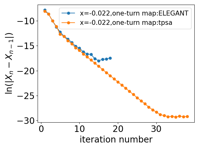
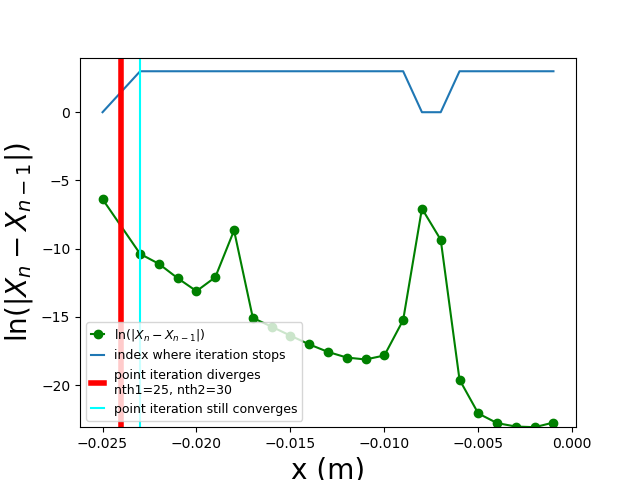
Figure 6: (a) $\delta X_{n}$ vs. iteration number $n$; (b) Minimum of $\delta X_{n}$ vs. $x$ , the red line is where iteration diverges for both $n_{\theta}=$25 and 30 and the maximum number of iteration is set at 4.

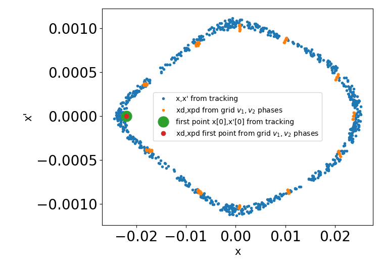
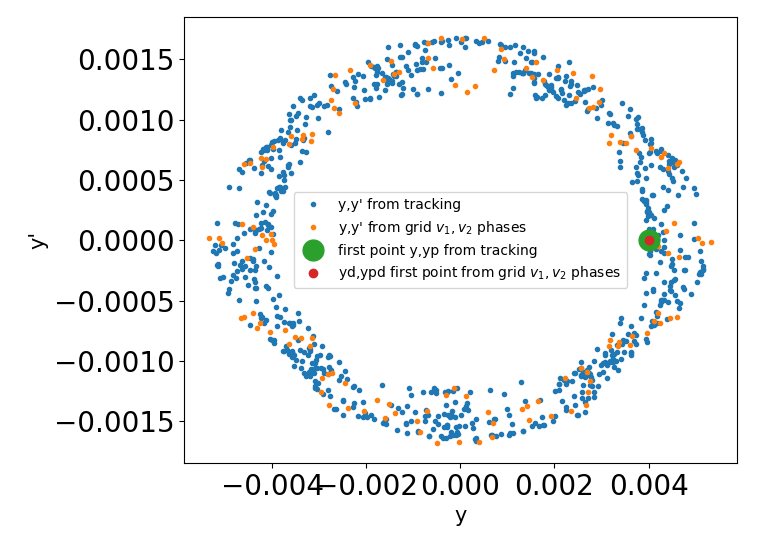
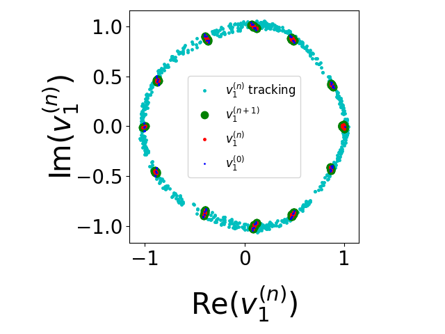
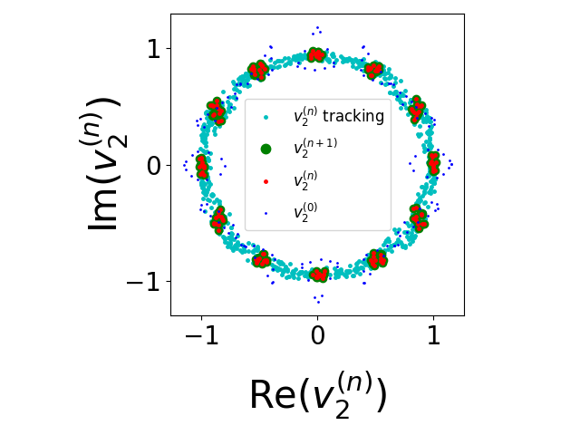
Figure 7: (a) trajectory in $xp_{x}$ plane within the range $-3mm<y<3mm$.  (b) trajectory in $yp_{y}$ plane within the range $-2mm<x<2mm$, blue (tracking by ELEGANT), orange (square matrix iteration). (c) trajectory in $v_{1}$ plane, (d) trajectory in $v_{2}$ plane. light blue (tracking by ELEGANT), red (square matrix iteration)

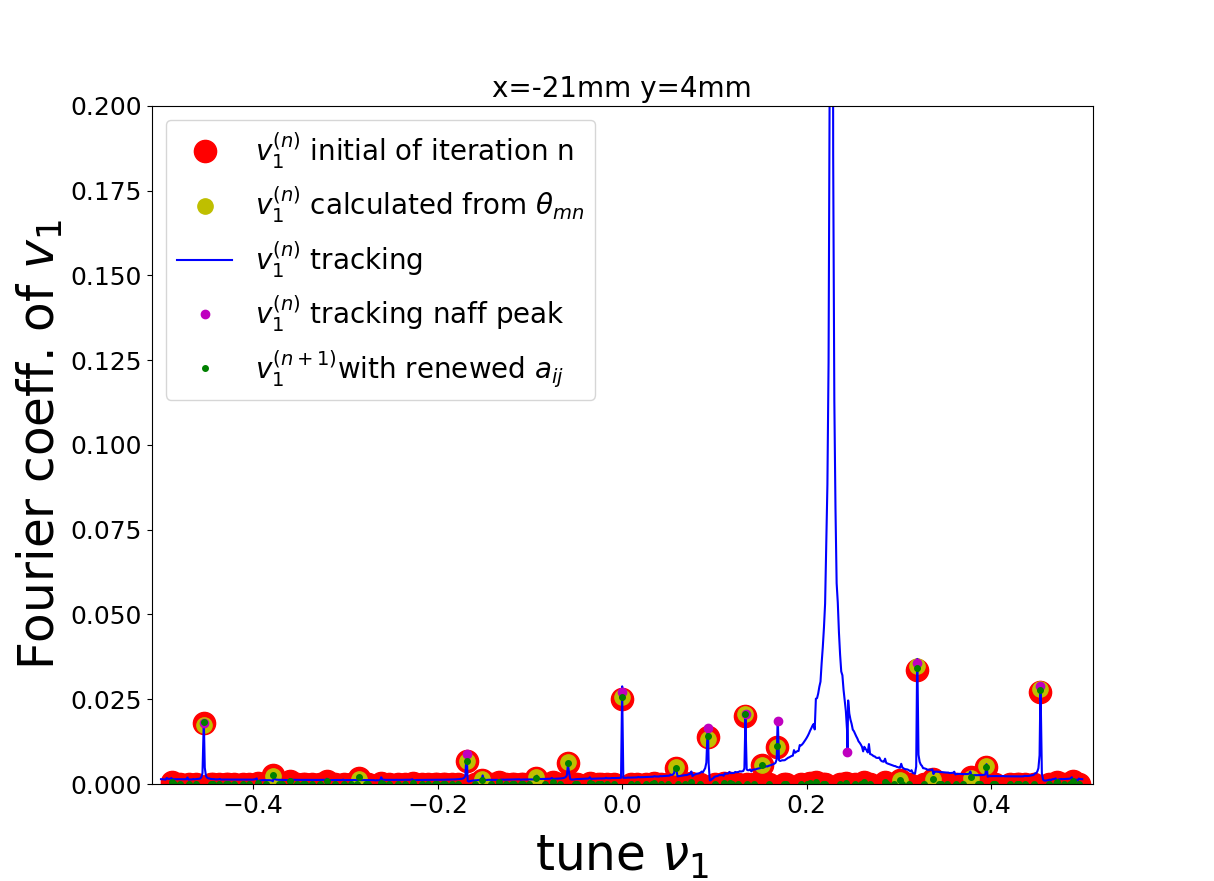
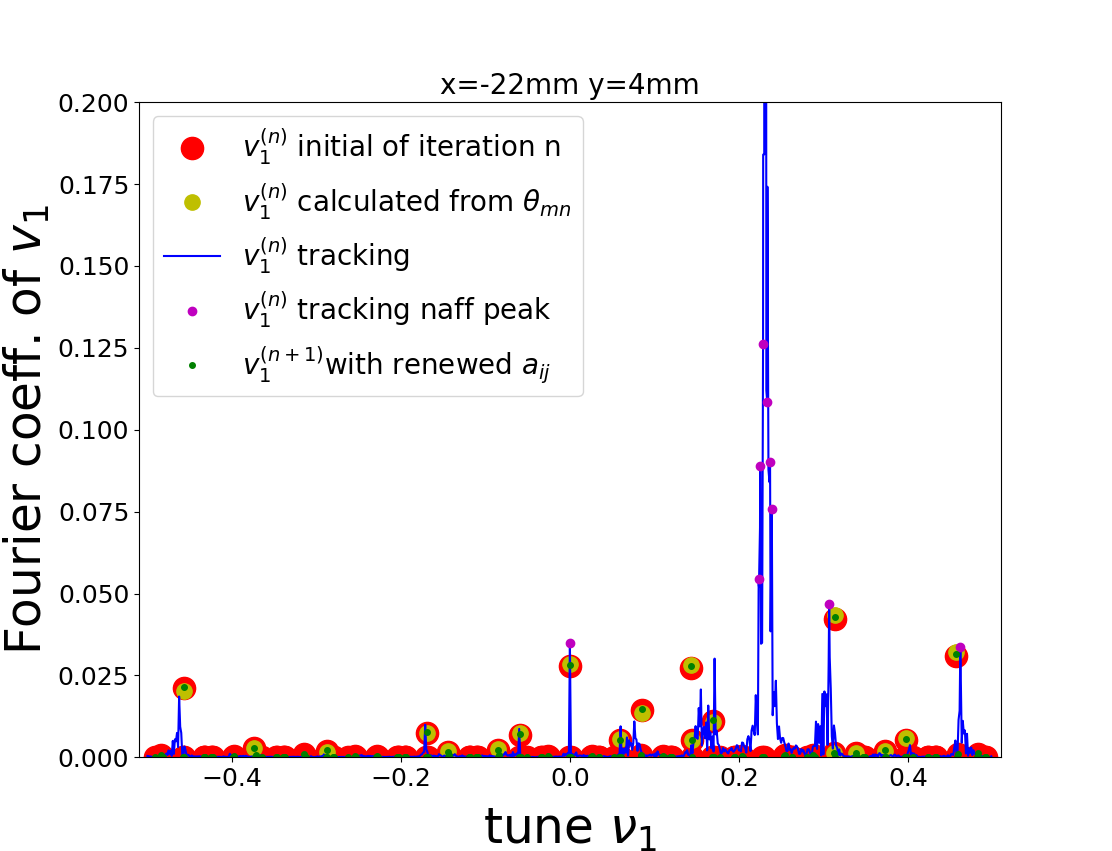
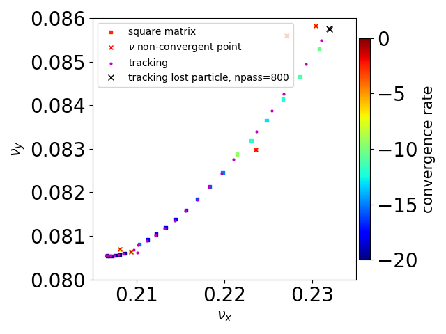
Figure 8: (a) and (b): spectrum of $v_{1}^{(n)}$ at the last iteration $4$ (red, yellow, green) compared with tracking (FFT from tracking blue, NAFF from tracking magenta) for $x=-21mm$ and $-22mm$ respectively. In order to see the precision of the spectrum, the vertical limit is 0.2 so the peak at nearly amplitude 1 is outside the scale and invisible. (c) tune footprints in $\nu_{x},\nu_{y}$ plane. (d) $\nu_{x}$ vs. $x$

In the following example of numerical application of the iteration steps in Section III, we use the matrix $M$ derived from one of the lattices for NSLSII storage ring. To construct the square matrix $M$, we first transform $x,p_{x},y,p_{y}$ to Courant-Snyder variables $z_{x}=\overline{x}-i\overline{p}_{x}$, $z_{y}=\overline{y}-i\overline{p}_{y}$, which are used to construct the monomial column $Z$. The the square matrix $M$ is construct from lattice input file using Truncated Power Series Algebra (TPSA) Berz (1989); Dragt (1988); Forest et al. (1989); Forest (1998); Chao (2002); Bazzani et al. (1994). We use four polynomials $w_{x0},w_{x1},w_{y0},w_{y1}$ derived from Jordan vector of power order 3, and corresponding linear combination coefficients $\{a_{1j}^{(k)},a_{2j}^{(k)}\},j=1,2,3,4$. Initially we take $a_{1}=1,0,0,0$, $a_{2}=0,0,1,0$. So initially we only use $w_{x0},w_{y0}$ for $v_{1}$ and $v_{2}$ respectively. During the iteration the contribution from $a_{12,}a_{13,}a_{14,}a_{21,}a_{22},a_{24}$ (starting from iteration $0$) increases to minimize the deviation of $v_{1}$ and $v_{2}$ from pure rotation, and improves the precision of $X^{(k)}$ so it is closer to real trajectory.

For a trajectory starting from $x=-22mm,y=4mm$, and momentum deviation $\delta=-0.025$ very close to dynamic aperture, when we take $n_{\theta}=12$, the iteration leads to convergence as shown in Fig.6a. When we use tracking by the code ELEGANT Borland (2000) to calculate the one turn map from $X_{k}$ to $X_{k+1}$, as mentioned in the definition of one turn mapping function $\phi_{1},\phi_{2}$ in Eq. (21), the minimum of $\ln(\delta X_{n})$ (blue) is -17 at the iteration 15 because the digital noise (order of $e^{-17}=4\times 10^{-8}$ mm) limited by the 7 digits in ELEGANT output ascii file we used. When we detect the minimum we stopped the iteration at step 18. Another way is to use square matrix of power order 5, the result is the orange dots (“tpsa”) with the minimum of $\ln(\delta X_{n})$ at -29.4 at iteration 32 (order of $e^{-29.4}=1.7\times 10^{-13}$ mm). Notice that even though the Jordan vector for the action-angle variables is of power order 3, the one turn map can be exact, as given by ELEGANT tracking. The results have almost same convergence rate, and at the the iteration 18, the trajectory difference is very small (order of $e^{-17}=4\times 10^{-8}$ mm). In the following, we we use square matrix of power order 3 to obtain the 3rd order polynomials of Jordan form. However in the iteration steps, the one turn map is calculated by the power order 5 square matrix (the calculation is approximate) to study the iteration convergence rate. As we mentioned before, the difference between using ELEGANT (the precise method) or power order 5 square matrix (the approximate method) is negligible in the optimization of the lattice.

For a scan from $x=$ -1mm to -26mm for every mm, we plot the minimum $\ln(\delta X_{n})$ of iteration for each $x$ in Fig.6b, here $n_{\theta}=12$. Because in Fig.6b our goal is only to study convergence, not to reach very high precision for the orbit, the maximum iteration is set at 4. The blue curve at the top is the number of iterations reached vs. $x$. For $x<-25mm$, and for $x=7,8$ mm the iteration diverges while for other $x$ the iteration converges. The vertical red line and light blue line in Fig.6b provide information about dynamical aperture and the relation between divergence and $n_{\theta}$ , to be addressed in Section V. The divergence at $x=7,8$ mm is due to resonance, where the trajectories move around two 1D-tori and form two islands in the 4D phase space. The 1D-tori can also be calculated to very high precision by square matrix method while trajectories in the resonance region are organized around the 1D-tori. However, the study around resonance region will be discussed in a separate publication.

The same iteration for initial value over the $xy$ plane with initial value of $p_{x},p_{y}=0,$ and momentum $\Delta p=0$ is shown in Fig.1a (before the Introduction) with $n_{\theta}=12$. The minimum of $\ln\delta X_{n}$ is represented by the color scale. The white area represents divergence of the iteration. We refer this map as a convergence map. A comparison of speed of the convergence map calculation with that of the frequency map will be discussed in Section VI. These two maps are entirely different maps, but both provide similar space structure. This suggests that the convergence map can be used in the nonlinear lattice optimization.

We use one point as an example of the iteration result, i.e. initial value $x=-22mm,y=4mm,\delta=-2.5\%$ Fig.7a,b compare trajectory calculated from ELEGANT and from iteration 4. Fig.7c,d show the trajectory in $v_{1}$ and $v_{2}$ complex plane respectively. Dark blue dots represent initial trial $v_{1}^{(0)}$ ,$v_{2}^{(0)}$ calculated with initial $\theta_{1}^{(0)}(\alpha),\theta_{2}^{(0)}(\alpha)$ and $n_{\theta}=12$. The red dots represent the result of $v_{1}^{(n)},v_{2}^{(n)}$ at the end of the iteration. The light blue lines represent $v_{1}^{(n)}$ ,$v_{2}^{(n)}$ calculated from tracking trajectory $x,p_{x},y,p_{y}$ for 1024 turns. There is a very good agreement between tracking and iteration results.

The spectrum of $v_{1}^{(n)}$ for $x=-21mm$ and $-22mm$ are shown in Fig.8 a,b. The main peaks are normalized to 1. The fluctuation peaks (red $v_{1}^{(k)}$ , yellow calculated from $\widetilde{\theta}_{1hm}$ and green $v_{1}^{(n+1)}$ dots) agree with tracking (blue lines) with peak (magenta dots) calculated by naff from tracking agree well even with limited $n_{\theta}=12$ for $x=-21mm$. For $x=-22mm,$ the difference is larger but the agreement is still very good considering the particle lost at $N=5448$. In Fig 8.c,d the tune footprint in $\nu_{x},\nu_{y}$ plane, and the $\nu_{x}$ vs. $x$ plot, the square matrix tune at the last iteration agree well with tracking except for points where the iteration diverges or particle lost in the tracking (represented by crosses).

In tracking for much longer time, the particle lost at $N=$5448 turns. Similarly when $n_{\theta}$ increased to 17, the iteration diverges.

There is a qualitative relation between the $n_{\theta}^{2}$ when iteration diverges and the number of turns $N$ when particle lost, obtained from numerical experiences. We have some intuitive understanding of this relation, but lack an analytical analysis so far, as will be addressed later in Section VII.

V An Example of Nonlinear Lattice Optimization

As a practical example for the utility of convergence maps (CMs), we used optimization of harmonic sextupoles for NSLS-II to maximize its on-momentum dynamic aperture (DA).

The lattice used for this was one super-period of NSLS-II (15 super-periods in the whole ring) without any insertion devices (often referred to as “ bare lattice”). The knobs for this optimization problem were the strengths for all 6 families of harmonic sextupoles. For each set of sextupole values, the DA, defined to be the maximum radius within which the convergence value stays below -12, was searched for each radial line. Nine radial lines covered the upper half-plane of x-y initial coordinate space. Each radial line search progressed monotonically outward with a step size of 1 mm, and stopped once the threshold convergence value was exceeded. These radial DA values were then used directly as the multi-objectives for the optimization problem.

The optimization algorithm employed for this problem was MOGA (multi-objective genetic algorithm) Deb (2001); Yang et al. (2011) implemented with DEAP Python package Fortin et al. (2012); DEA .

Figure 9a shows the frequency map (FM) of one of the optimal lattices after CM optimization. As in the previous section, the FMs in this section were generated by the “frequency map” command of ELEGANT Borland (2000). The magenta circles correspond to the 9 radial apertures found by CM during the optimization process. The full convergence map for the same lattice is shown in Fig. 9b, whose boundary looks similar to that of the FM. The horizontal aperture (near y=0) extends up to -30 mm and +35 mm, while satisfying the minimum required 2-mm vertical DA. In this sense, this optimized lattice appears to be better than the NSLS-II bare lattice whose FM and CM are shown in Fig. 1a,1b.

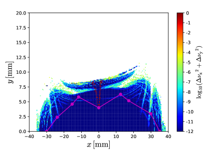
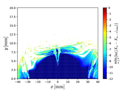
Figure 9: (a)The frequency map and the radial apertures (magenta circles) found by convergence map for one of the optimized lattices. (b) The full convergence map for the same lattice and on the same grid used in (a).

This CM optimization was also able to find a lattice, shown in Fig.10 whose FM and CM appear very similar to those of NSLS-II bare lattice shown in Fig. 1. These two optimized lattices shown in Fig.9 and Fig.10 demonstrate that the optimization based on CM can find lattices at least as good as or better than the optimization using DA based on many-turn particle survival. Furthermore, it achieves this feat with only a fraction of the computation resources.

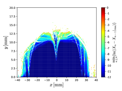
Figure 10: (a)The frequency map and (b) the convergence map for an optimized lattice similar to NSLS-II bare lattice

VI Computation Time Comparison of Convergence Map vs. Frequency Map

Computation time was compared between the convergence map and the frequency map using one super-period (2 cells) and the whole ring (15 super-period) of the NSLS-II bare lattice. By “bare” , it means there is no insertion device element in the lattice.

To compare the two maps, we need to compare the computation time for selected points in x-y plane in the NSLS-II bare lattice. If we choose the points in an unstable region, some particles may be lost during tracking. This would make the comparison difficult.

For a fair comparison, we chose a stable region. For both types of maps, an initial coordinate region of $+10\leq x[\text{mm}]\leq+11$ and $+1\leq y[\text{mm}]\leq+2$ was selected as particles launched from this region are very stable and can last at least 1024 turns specified for frequency map analysis. This square region was divided into $2\times 2$, $3\times 3$, $5\times 5,10\times 10,50\times 50,100\times 100$ grid points as a set of different number of points. Each grid point is used as an initial transverse coordinate for both maps. The momentum offset was zero.

For frequency map computations, we used ELEGANT “frequency_map” command Borland (2000) to compute the diffusion defined by the tune changes between the first 512 and the latter 512 turns.

For convergence map computations, PyTPSA PyT was used to create truncated power series (TPS) objects and handle all the algebraic operations on them while the TPS objects are propagated through all the lattice elements in a Python module where the symplectic integration method of TRACY J. Bengtsson has been reimplemented. The components of the TPS have been confirmed with simulation code MADX-PTC Skowronski et al. . During the speed test we use $n_{\theta}=12$. The number of iteration is set at 4. The polynomials $w_{j}=u_{j}Z,$ based on Jordan form as introduced by Eq. (13), are polynomials of 3rd power order. For readers who might be interested in the detailed implementation of our method, please see sqm .

All the computations in this section were performed using a single core of Intel Xeon Gold 6252 CPU at 2.10 GHz (hyper-threading enabled). The results are shown in Fig. 2 in the Introduction.This proposed CM method is also friendly to parallelization, which has been demonstrated to scale well to 128 cores.

The computation time of frequency maps (FM) linearly scaled with the number of grid points as expected. It was also expected to linearly scale with the number of super-periods (SP), as each point requires tracking of a single particle from the beginning to the end of the selected lattice. Thus, the whole-ring lattice should have taken roughly 15 times longer than the 1-SP lattice. However, the time only increased by 10.5. This appears to indicate the overhead of non-tracking portion of ELEGANT code is not negligible, compared to the tracking portion.

The most notable feature of the convergence map (CM) time is the fact that it changed very little for the case of $10^{4}$ points whether the lattice was 1 or 15 super-periods. This makes sense because once the TPSA calculation for a lattice is finished at the beginning, the computation cost is the same for each grid point, whether the lattice was 1 or 15 super-periods, unlike the tracking-based FM whose computation time is proportional to the length of the lattice. Note that the initial TPSA calculation does depend on the length of the lattice. However, it only increased from 0.81 s for 1 SP to 6.45 s for 15 SP. In both cases, this initial setup time is tiny compared to the total time of 100 seconds it took to compute the convergence values for $10^{4}$ points.

The speed of CM for $10^{4}$ points was 31.2 times faster than that of FM for the 1-SP case, while it was 314 times faster for the 15-SP case. These speed improvement factors include all the overhead and initial setup times. However, the advantage of CM diminishes as the number of points decrease, since the initial TPSA computation time starts to dominate the total CM computation time. Therefore, CM is particularly useful when the number of initial coordinate points whose stability needs to be investigated is quite large and/or when the lattice under study is very long and complex (e.g., lattices with multipole and alignment errors included and lattices with no periodicity such as colliders).

The dashed lines in Fig. 2 shows the computation times for CM without the initial setup times. Both the 1-SP and 15-SP curves show good linearity with the number of grid points. They are also almost on top of each other. This demonstrates the earlier statement of the convergence value computation time being independent of the lattice length/complexity, as long as the initial TPSA computation time is excluded.

VII Survival turn number $N$ and Dynamic Aperture, and its Relation to Convergence-Divergence-$n_{\theta}$ Dependence

Frequency map and convergence map are very different but related. In a frequency diagram, the dynamical aperture is given by the boundary where the particle is lost within a specified number of turns $N$. To find dynamical aperture defined by the divergence of the iteration by square matrix method, we need to understand the relation between divergence of the iteration and $n_{\theta}$.

The survival turn number is very sensitive to initial position $x$, so the study is based on statistical average. In Fig.11.a, the number of survival turns is plotted vs. $x$ for every 0.1mm, and for every 0.1mm with neighbour 20 points separated by $10\mu m$, tracking $N=65536$ turns. There is a boundary at $x=$-21.2mm if we choose $N=60000$, and the very thin area at $x=-22.8mm$. But for application in light source, with damping time about 10ms, if we take $N=1024$, then Fig.11.b (the same plot as Fig.11a with vertical range reduced to 10000 ) shows fluctuation of the number of survival turns is so large, that we need to further average over a certain range of $x$. Fig.11c shows the result of averaging over every 20 points of neighbour $x$ and compared with the same set of data in Fig.11b, the dynamical aperture is about $x=-23mm$. Similar plot is shown in Fig.11d with more points of average gives less fluctuation.

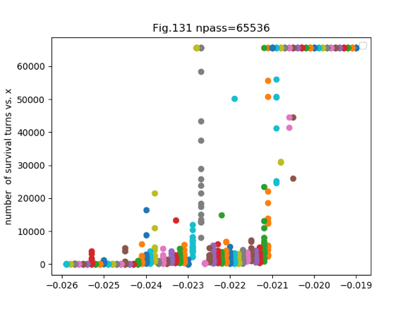
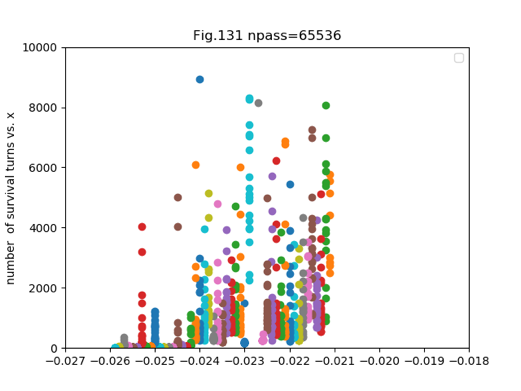
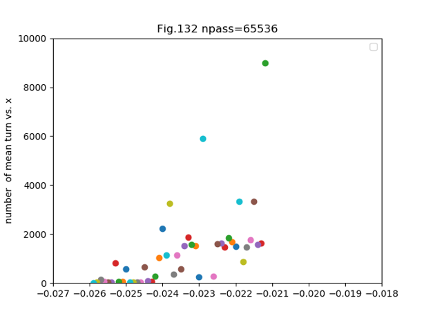
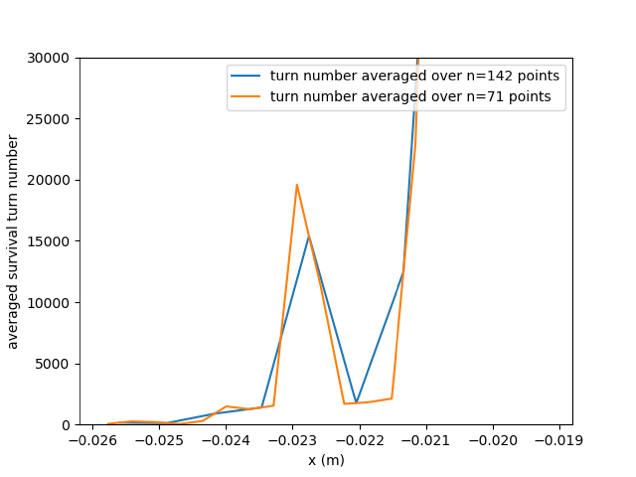
Figure 11: a and b: number of survival turns vs. $x$ by tracking ELEGANT in 70000 and 10000 scale c: same plot averaged over every 20 points of neighbour $x$ d: same plot averaged over 0.35mm (orange) and 0.7 mm (blue) respectively

Similarly, we can use the convergence-divergence-$n_{\theta}$ dependence in iteration by square matrix method to estimate the dynamical aperture. Fig.12 a,b are the 3D plot of iteration convergence rate vs. $n_{\theta}$ for $x=-20.1mm,20.2mm$ respectively. At $x=-20.1mm$ the iterations are convergent from $n_{\theta}=25$ to $80$ with only exception at $n_{\theta}=68,72$. But at $x=-20.2mm$ the iterations diverge for all $n_{\theta}>35$. Numerical study for many different $x$ shows when $n_{\theta}$ increases above a certain number, the divergence points form a continuous band with only very few points convergent.

The lowest point $n_{\theta}$ of the divergence band is also sensitive to $x$. Similar to tracking, Fig.12c plot the points of $n_{\theta}^{2}$ where the iteration converges. The distribution is also sensitive to the initial $x$, and Fig.12b shows at $x=-20.2$ there are band of divergence points above $n_{\theta}>40$. To be able to estimate dynamical aperture from this data, again, the $n_{\theta}^{2}$ is averaged over a small range of $x$ for every point, and plotted in Fig.12d. Compared with Fig.11d, Fig.12d also show that there is fast decrease of convergence at $x=-20.2mm$. If we take divergence at $n_{\theta}>25$ for aperture, then the aperture is estimated at $x=-21mm$. For crude estimate we may take $n_{\theta}=12$, then the aperture would be estimate as $x=-22mm$. This example indicates that even with relatively low $n_{\theta}=12$ the dynamical aperture is within $1mm$ from the aperture obtained by tracking of 6000 turns.

There is a resonance line at $x=-18.6mm$, an indication the iteration convergence is sensitive to resonance. A more detailed calculation leads to convergence at this point, but the calculation takes some more time. Since the main goal of this paper is to study dynamical aperture, the resonance study will be addressed in future publication. As we mentioned in regard of Fig.6b, near the resonance center, the square matrix method can also be applied to obtain very accurate information about a 1D-torus. Even though qualitatively we can use the convergence map to estimate the dynamical aperture, we still lack a more quantitative analytical understanding of the relation between iteration convergence at $n_{\theta}$ and particle loss at turn $N$. The fact that Fig.12c seems to be a little more regular than Fig.11b indicates that there might be some analytical way to explain the statistics of divergence vs. $n_{\theta}.$

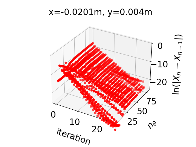
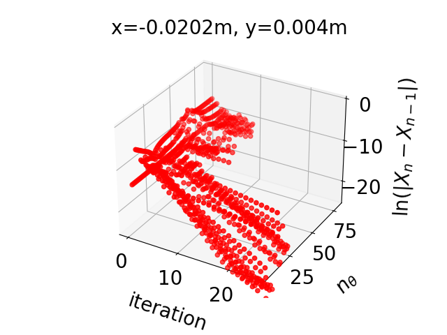
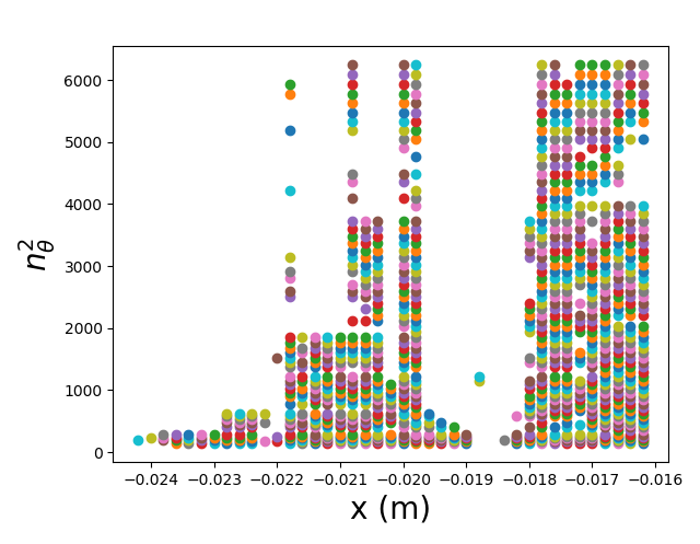
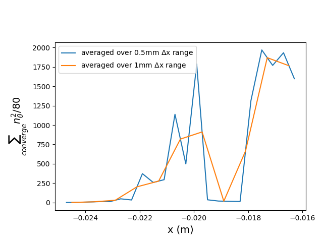
Figure 12: (a) the 3D plot of iteration convergence rate vs. $n_{\theta}$ for a: $x=-20.1mm.(b),x=-20.2mm$. (c) $n_{\theta}^{2}$ vs. x. (d) $n_{\theta}^{2}$ averaged over 80 points of neighbour $x$.

The comparison of Fig.12d and Fig.11d indicates the possibility of using convergence map to study dynamical aperture. Hence the speed of the calculation is important, as discussed in Section V.

VIII Conclusion

In this paper we show that the action-angle variables derived from square matrix method is close to a pure rotation, hence it is possible to rewrite the nonlinear dynamical equations in terms of these variables as an exact equation. The equation is in the form of pure rotation with nonlinear terms as perturbation. Hence an iteration steps developed using perturbation method to solve the nonlinear dynamical equation are convergent up to dynamic aperture or the border of resonance region. The convergence rate varies depending on how close the trajectory is to the dynamic aperture or resonance region. Hence the convergence rate is a function of the initial particle coordinates. For example the convergence rate can be plotted as a function of horizontal and vertical coordinates, as a color map. This “convergence map” can be used to study the stability of the nonlinear system.

This convergence map is similar but very different from frequency map calculated by tracking. The results agree with tracking well on dynamic aperture, tune footprint and phase space trajectory, and frequency spectrum to high precision. Using an NSLS-II lattice as an example, we carried out an extensive comparison of the optimization by traditional tracking method with the convergence map. We compared the speed and the quality of the optimization result, and show that depends on the complexity of the lattices. The iteration method is about 30 to 300 times faster than tracking.

Hence the convergence map is suitable for nonlinear optimization of storage ring lattice, and in particular for the study of the very long term behavior in storage rings with very large number of sextupoles or high order multipoles.

Appendix A Fourier Transform Solution of Iteration Equation

We write the two dimensional Fourier transform of $\phi_{1}(\alpha_{1},\alpha_{2}),\phi_{2}(\alpha_{1},\alpha_{2}),\theta_{1}(\alpha_{1},\alpha_{2}),\theta_{2}(\alpha_{1},\alpha_{2})$ in Eq. (25) (the iteration number $k$ is implicitly implied) as:

$$\begin{split}&\phi_{1}(\alpha_{1},\alpha_{2})=\omega_{1}+\sum_{\tiny{\begin{matrix}m,n\\ |n|+|m|\neq 0\end{matrix}}}^{n_{\theta},n_{\theta}}\widetilde{\phi}_{1nm}e^{in\alpha_{1}}e^{im\alpha_{2}},\phi_{2}(\alpha_{1},\alpha_{2})=\omega_{2}+\sum_{\tiny{\begin{matrix}m,n\\ |n|+|m|\neq 0\end{matrix}}}^{n_{\theta},n_{\theta}}\widetilde{\phi}_{2nm}e^{in\alpha_{1}}e^{im\alpha_{2}}\\ &\theta_{1}(\alpha_{1},\alpha_{2})=\alpha_{1}+\sum_{n,m=0,0}^{n_{\theta},n_{\theta}}\widetilde{\theta}_{1nm}e^{in\alpha_{1}}e^{im\alpha_{2}},\theta_{2}(\alpha_{1},\alpha_{2})=\alpha_{2}+\sum_{n,m=0,0}^{n_{\theta},n_{\theta}}\widetilde{\theta}_{2nm}e^{in\alpha_{1}}e^{im\alpha_{2}}\end{split}$$ (27)

where in the sum in $\phi_{1},\phi_{2}$ the indexes run from $0$ to $n_{\theta}$ except the term for $m=n=0$, i.e., the constant terms are removed and replaced by $\omega_{1},\omega_{2}$ respectively. Compare both sides of the Fourier transform of the first equation in Eq. (23) leads to

$$\alpha_{1}+\omega_{1}+\sum_{n,m=0,0}^{n_{\theta},n_{\theta}}\widetilde{\theta}_{1nm}e^{in(\alpha_{1}+\omega_{1})}e^{im(\alpha_{2}+\omega_{2})}-\alpha_{1}-\sum_{n,m=0,0}^{n_{\theta},n_{\theta}}\widetilde{\theta}_{1nm}e^{in\alpha_{1}}e^{im\alpha_{2}}\approx\omega_{1}+\sum_{\tiny{\begin{matrix}m,n\\ |n|+|m|\neq 0\end{matrix}}}^{n_{\theta},n_{\theta}}\widetilde{\phi}_{1nm}e^{in\alpha_{1}}e^{im\alpha_{2}}$$

$$\sum_{n,m=0,0}^{n_{\theta},n_{\theta}}\widetilde{\theta}_{1nm}e^{in(\alpha_{1}+\omega_{1})}e^{im(\alpha_{2}+\omega_{2})}-\sum_{n,m=0,0}^{n_{\theta},n_{\theta}}\widetilde{\theta}_{1nm}e^{in\alpha_{1}}e^{im\alpha_{2}}\approx\sum_{\tiny{\begin{matrix}m,n\\ |n|+|m|\neq 0\end{matrix}}}^{n_{\theta},n_{\theta}}\widetilde{\phi}_{1nm}e^{in\alpha_{1}}e^{im\alpha_{2}}$$

$$\sum_{n,m=0,0}^{n_{\theta},n_{\theta}}\widetilde{\theta}_{1nm}e^{i(n\omega_{1}+m\omega_{2})}e^{in\alpha_{1}}e^{im\alpha_{2}}-\sum_{n,m=0,0}^{n_{\theta},n_{\theta}}\widetilde{\theta}_{1nm}e^{in\alpha_{1}}e^{im\alpha_{2}}\approx\sum_{\tiny{\begin{matrix}m,n\\ |n|+|m|\neq 0\end{matrix}}}^{n_{\theta},n_{\theta}}\widetilde{\phi}_{1nm}e^{in\alpha_{1}}e^{im\alpha_{2}}$$

$$\widetilde{\theta}_{1nm}e^{i(n\omega_{1}+m\omega_{2})}-\widetilde{\theta}_{1nm}\approx\widetilde{\phi}_{1nm}$$

$$\widetilde{\theta}_{1nm}=\frac{\widetilde{\phi}_{1nm}}{e^{i(n\omega_{1}+m\omega_{2})}-1}$$

$$\widetilde{\theta}_{2nm}=\frac{\widetilde{\phi}_{2nm}}{e^{i(n\omega_{1}+m\omega_{2})}-1}$$ (28)

for $\text{ (}|n|+|m|\neq 0),$i.e, except the constant terms. For the constant terms, both sides are zeros so there we still need to find $\widetilde{\theta}_{100},\widetilde{\theta}_{200}$ from other condition. They are determined by the condition that the second line of Eq. 27 must be valid for $\alpha_{1}\equiv k\omega_{1}+\theta_{10},\alpha_{2}\equiv k\omega_{2}+\theta_{20}$ with all $k$ including $k=0$, i.e., when $\theta_{10}(\theta_{10},\theta_{20})=\theta_{10},\theta_{20}(\theta_{10},\theta_{20})=\theta_{20}$ so

$$\begin{split}&\theta_{10}=\theta_{10}+\sum_{n,m=0,0}^{n_{\theta},n_{\theta}}\widetilde{\theta}_{1nm}e^{in\theta_{10}}e^{im\theta_{20}}\text{ }\\ &\theta_{20}=\theta_{20}+\sum_{n,m=0,0}^{n_{\theta},n_{\theta}}\widetilde{\theta}_{2nm}e^{in\theta_{10}}e^{im\theta_{20}}.\end{split}$$ (29)

Hence

$$\begin{split}&\widetilde{\theta}_{100}=-\sum_{\tiny{\begin{matrix}m,n\\ |n|+|m|\neq 0\end{matrix}}}^{n_{\theta},n_{\theta}}\widetilde{\theta}_{1nm}e^{in\theta_{10}}e^{im\theta_{20}}\\ &\widetilde{\theta}_{200}=-\sum_{\tiny{\begin{matrix}m,n\\ |n|+|m|\neq 0\end{matrix}}}^{n_{\theta},n_{\theta}}\widetilde{\theta}_{2nm}e^{in\theta_{10}}e^{im\theta_{20}}\end{split}$$ (30)

During the $k^{\text{th}}$ iteration, $\widetilde{\phi}_{1nm},\widetilde{\phi}_{1nm},\omega_{1},\omega_{2}$ of the right hand side should be label as $(k)$, while $\widetilde{\theta}_{1nm},\widetilde{\theta}_{2nm}$ of the left hand side should be labeled as $(k+1)$, as labeled in Eq. (25). Thus the inverse Fourier transform gives the solution $\theta_{1}^{(k+1)}(\alpha_{1},\alpha_{2}),\theta_{2}^{(k+1)}(\alpha_{1},\alpha_{2})$. In the numerical calculation, $\alpha_{1},\alpha_{2}$ are only specified at discrete $n_{\theta}\times n_{\theta}$ points on the $\alpha_{1},\alpha_{2}$ torus plane of period $(2\pi\times 2\pi)$.

Appendix B Calculation of Linear Combinations using a known trajectory

Near the elliptical fixed point, the dynamics is dominated by the linear terms $z_{x},z_{y}$ in the square matrix $M,$ so $w_{x0}(X)$ and $w_{y0}(X)$ are near exact action-angle variables, and carry out nearly a pure rotation independently with linear tune $\mu_{x},\mu_{y}$ respectively. The coefficients $\{a_{ij}\}$ in Eq.(26) can be chosen as $a_{11}^{(0)}=1,a_{23}^{(0)}=1$ while all other $a_{ij}^{(0)}=0$ for the first iteration step. In the case of increased amplitude, these coefficients are determined by $x$,$p_{x}$,$y$,$p_{y}$ in a larger neighborhood near the fixed point. Obviously, the high power terms in Eq.(12) serve as a perturbation to the rigid rotation. (For a much more detailed and rigrorous description we refer to Poincare-Birkhoff theorem Brown and Neumann (1977)). During the iteration, the higher power terms in $w_{x1}(X),w_{y0}(X),w_{y1}(X)$ contribute to the deviation of $v_{1}$ from a pure rotation, and the same way $w_{x0}(X),w_{x1}(X),w_{y1}(X)$ contribute to the deviation of $v_{2}$. Hence $a_{ij}^{(0)}$ can be further minimized by a least square method to $a_{ij}^{(1)}$ as a starting point of the second iteration step. This can be continued for every iteration step $k$ for $a_{ij}^{(k)}$. Our experience shows renew $a_{ij}^{(k)}$ in each iteration step makes the convergence faster.

In the following we shall show that if we have a numerical direct integration of the dynamical equations, i.e., if we have the trajectory $X^{(k-1)}$, we can use the Fourier expansion of $w_{xi}(X^{(k-1)}),w_{yi}(X^{(k-1)})$ to determine the linear combinations $a_{ij}^{(k)}$ that minimize the deviation from pure rotation for the approximate rigid rotation $v_{1},v_{2}$. Hence an approximate trajectory can be used to determine the linear combinations by a least square method.

For a trajectory $\theta_{1}^{(k-1)}(\alpha_{1},\alpha_{2}),\theta_{2}^{(k-1)}(\alpha_{1},\alpha_{2})$, i.e., the solution of Eq. (25), the coordinates $X^{(k-1)}$ can be found by the inverse function of Eq. (26), as functions of $\alpha_{1},\alpha_{2}$ (modulo $2\pi$), hence the eigenvectors $w_{x0}$ , $w_{x1}$, $\ldots$ can also be Fourier expanded in terms of $\alpha_{1},\alpha_{2}$.

For simplicity in writing, if we choose $n_{v}$ eigenvectors for the linear combinations, we label them as $w_{j}$ with $j=1,2,..,n_{v}$. For example, for Eq.(26), $n_{v}=4$, $w_{1}\equiv w_{x0},w_{2}\equiv w_{x1},$ $w_{3}\equiv w_{y0},w_{4}\equiv w_{y1}$. We have the expansion

$$w_{j}(\alpha_{1},\alpha_{2})=\sum_{n,m}\widetilde{w}_{jnm}e^{in\alpha_{1}}e^{im\alpha_{2}}\qquad(j=1,2,..n_{v})$$ (31)

Here $m,n=0,1,2,...,n_{\theta}$ see Eq.(27). Now we look for linear combinations $a_{1j}$,$a_{2j}$ to construct the two approximate action-angle variables $v_{1},v_{2}$

$$v_{l} =\sum_{j=1}^{n_{v}}a_{lj}w_{j}=\sum_{n,m}\left(\sum_{j=1}^{n_{v}}a_{lj}\widetilde{w}_{jnm}\right)e^{in\alpha_{1}}e^{im\alpha_{2}}$$ (32)

$$\equiv\sum_{n,m}\widetilde{v}_{lnm}e^{in\alpha_{1}}e^{im\alpha_{2}}\qquad(l=1,2)$$

The Fourier coefficient for spectral line $n\omega_{1}+m\omega_{2}$ is $\widetilde{v}_{lnm}=\sum_{j}a_{lj}\widetilde{w}_{jnm}$. We choose $a_{lj}$ such that $\widetilde{v}_{110}=1$, $\widetilde{v}_{201}=1$, and define $\widetilde{v}_{1nm}=\epsilon_{1nm}$, for all ${n,m}$ except ${n=1,m=0}$, and $\widetilde{v}_{2nm}=\epsilon_{2nm}$ for all ${n,m}$ except for ${n=0,m=1}$. $\epsilon_{lnm}$ represents fluctuation. Among all possible values for $a_{lj}$, the one with minimized fluctuation most closely represents the rigid rotations. In general, we have a minimization problem for a function $g_{0}$ quadratic in $a_{lj}$ with constraints $g_{1},g_{2}$:

$$g_{0}(a_{lj})=\sum_{\tiny{\begin{matrix}n,m\\ |n-1|+|m|\neq 0\end{matrix}}}|\epsilon_{1nm}|^{2}+\sum_{\tiny{\begin{matrix}n,m\\ |n|+|m-1|\neq 0\end{matrix}}}|\epsilon_{2nm}|^{2}$$ (33)

$$g_{1}(a_{lj})=\widetilde{v}_{110}-1=0$$

$$g_{2}(a_{lj})=\widetilde{v}_{201}-1=0$$

If $g_{0}=0$, then $\epsilon_{lnm}$ are all zero, $v_{l}=e^{i\omega_{l}t}$ has a single frequency $\omega_{l}$, and $v_{1},v_{2}$ would be exact pure rotations. In general the fluctuation would not vanish, and for a finite power order $n_{s}$ of the square matrix (in this paper we found $n_{s}=3$ would give very accurate solution) and eigenvector number $n_{v}$ (in our example, we use $n_{v}=4$), we minimize the fluctuation $g_{0}$ to improve the action-angle variables as follows.

Use Lagrangian multiplier $\lambda_{1}$, $\lambda_{2}$, the minimization problem is reduced to solving $2n_{v}+2$ linear equations for $2n_{v}+2$ unknown $a_{lj,}$$\lambda_{1},\lambda_{2}$:

$$\frac{\partial g_{0}}{\partial a_{lj}}+\lambda_{1}\frac{\partial g_{1}}{\partial a_{lj}}+\lambda_{2}\frac{\partial g_{2}}{\partial a_{lj}}=0\qquad(l=1,2;\ j=1,2,..n_{v})$$ (34)

$$g_{1}=0,g_{2}=0$$

The solution of Eq.(34) is straight forward, and gives the linear combinations $a_{1k},a_{2k}$

$$a_{1h}=\frac{\sum_{j}\left(F_{1}^{-1}\right)_{hj}\widetilde{w}_{j10}^{*}}{\sum_{m,j}\widetilde{w}_{m10}\left(F_{1}^{-1}\right)_{mj}\widetilde{w}_{j10}^{*}}\qquad(m,j,h=1,2,..n_{v})$$

$$a_{2h}=\frac{\sum_{j}\left(F_{2}^{-1}\right)_{hj}\widetilde{w}_{j01}^{*}}{\sum_{m,j}\widetilde{w}_{m01}\left(F_{2}^{-1}\right)_{mj}\widetilde{w}_{j01}^{*}}\qquad\text{{with}}$$ (35)

$$\left(F_{1}\right)_{jh}\equiv\sum_{\tiny{\begin{matrix}n,m\\ |n-1|+|m|\neq 0\end{matrix}}}\widetilde{w}_{jnm}^{*}\widetilde{w}_{hnm}\qquad m,n=0,1,2, n_{\theta}$$(…,)

$$\left(F_{2}\right)_{jh}\equiv\sum_{\tiny{\begin{matrix}n,m\\ |n|+|m-1|\neq 0\end{matrix}}}\widetilde{w}_{jnm}^{*}\widetilde{w}_{hnm}\quad$$

For a given approximate trajectory $X^{(k-1)}(\alpha_{1},\alpha_{2})\equiv x^{(k-1)}$,$p_{x}^{(k-1)}$,$y^{(k-1)}$,$p_{y}^{(k-1)}$ as function of $\alpha_{1},\alpha_{2}$, the linear combinations $a_{1h}^{(k)},a_{2h}^{(k)}$ Eq.(35) determine the approximate action-angle variables $v_{1}^{(k)},v_{2}^{(k)}$ with minimized fluctuation Eq.(33), so they represent motion closer to pure rotations. Thus in every step of the iteration, the new solution not only closer to an exact solution of the exact dynamical equation Eq(23), it is also closer to a pure rotation. With less fluctuation from pure rotation, the convergence is faster.

References

- Lichtenberg and Lieberman (1992) A. J. Lichtenberg and M. Lieberman, Regular and Chaotic Dynamics (Springer, New York, 1992).
- Ruth (1987) R. D. Ruth, AIP Conf. Proc. 153, 150 (1987).
- Guignard (1978) G. Guignard, A general treatment of resonances in accelerators, CERN Academic Training Lecture (CERN, Geneva, 1978) cERN, Geneva, 1977 - 1978.
- Schoch (1958) A. Schoch, Theory of linear and non-linear perturbations of betatron oscillations in alternating-gradient synchrotrons, CERN Yellow Reports: Monographs (CERN, Geneva, 1958).
- Dragt (1988) A. J. Dragt, AIP Conference Proceedings 177, 261 (1988), https://aip.scitation.org/doi/pdf/10.1063/1.37819 .
- Berz (1989) M. Berz, in Proceedings of the 1989 IEEE Particle Accelerator Conference, . ’Accelerator Science and Technology (1989) pp. 1419–1423 vol.3.
- Chao (2002) A. Chao, “Lecture notes on topics in accelerator physics,” (2002).
- Bazzani et al. (1994) A. Bazzani, G. Servizi, E. Todesco, and G. Turchetti, A normal form approach to the theory of nonlinear betatronic motion, CERN Yellow Reports: Monographs (CERN, Geneva, 1994).
- Forest (1998) E. Forest, Beam Dynamics: A New Attitude and Framework (Harwood, Amsterdam, Netherlands, 1998).
- Forest et al. (1989) E. Forest, M. Berz, and J. Irwin, Part. Accel. 24, 91 (1989).
- Michelotti and Lifshitz (1995) L. Michelotti and E. M. Lifshitz, IntermediateClassical Dynamics with Applications to Beam Physics (Wiley, New York, 1995).
- (12) L.-H. Yu and B. Nash, in Proc. PAC’09 (JACoW Publishing, Geneva, Switzerland) pp. 3862–3864.
- Yu (2017) L. H. Yu, Phys. Rev. Accel. Beams 20, 034001 (2017).
- (14) L. H. Yu, Y. Hao, Y. Hidaka, F. Plassard, and V. V. Smaluk, in Proc. IPAC’21 (JACoW Publishing, Geneva, Switzerland) pp. 182–185.
- (15) Y. Hao, K. J. Anderson, and L. H. Yu, in Proc. IPAC’21 (JACoW Publishing, Geneva, Switzerland) pp. 3788–3791.
- Dierker (2007) S. Dierker, “Nsls-ii preliminary design report,” (2007).
- Nadolski and Laskar (2003) L. Nadolski and J. Laskar, Phys. Rev. ST Accel. Beams 6, 114801 (2003).
- (18) https://github.com/YueHao/PyTPSA.
- Wayne (1990) C. E. Wayne, Communications in Mathematical Physics 127, 479 (1990).
- Kågström and Ruhe (1980) B. Kågström and A. Ruhe, ACM Trans. Math. Softw. 6, 437–443 (1980).
- Kågström and Ruhe (1980) B. Kågström and A. Ruhe, ACM Trans. Math. Softw. 6, 398 (1980).
- Broer (2004) H. Broer, Bulletin of the American Mathematical Society 41, 1 (2004).
- Arnold (2009) V. Arnold, “Small denominators. i. mapping of the circumference onto itself,” (2009).
- Borland (2000) M. Borland, in 6th International Computational Accelerator Physics Conference (ICAP 2000) (2000).
- Deb (2001) K. Deb, “Multiobjective optimization using evolutionary algorithms. wiley, new york,” (2001).
- Yang et al. (2011) L. Yang, Y. Li, W. Guo, and S. Krinsky, Phys. Rev. ST Accel. Beams 14, 054001 (2011).
- Fortin et al. (2012) F.-A. Fortin, F.-M. De Rainville, M.-A. G. Gardner, M. Parizeau, and C. Gagné, J. Mach. Learn. Res. 13, 2171–2175 (2012).
- (28) https://github.com/DEAP/deap.
- (29) H. N. J. Bengtsson, E.Forest, Tracy User Manual.
- (30) P. K. Skowronski, E. Forest, F. Schmidt, and R. de Maria, in Proc. ICAP’06 (JACoW Publishing, Geneva, Switzerland) pp. 209–212.
- (31) https://github.com/yhidaka/squarematrix.
- Brown and Neumann (1977) M. Brown and W. D. Neumann, Michigan Mathematical Journal 24, 21 (1977).