Also at ]Department of Chemical Engineering, Carnegie Mellon University, Pittsburgh, PA 15213, USA
MeshDQN: A Deep Reinforcement Learning Framework for Improving Meshes in Computational Fluid Dynamics
Abstract
Meshing is a critical, but user-intensive process necessary for stable and accurate simulations in computational fluid dynamics (CFD). Mesh generation is often a bottleneck in CFD pipelines. Adaptive meshing techniques allow the mesh to be updated automatically to produce an accurate solution for the problem at hand. Existing classical techniques for adaptive meshing require either additional functionality out of solvers, many training simulations, or both. Current machine learning techniques often require substantial computational cost for training data generation, and are restricted in scope to the training data flow regime. MeshDQN is developed as a general purpose deep reinforcement learning framework to iteratively coarsen meshes while preserving target property calculation. A graph neural network based deep Q network is used to select mesh vertices for removal and solution interpolation is used to bypass expensive simulations at each step in the improvement process. MeshDQN requires a single simulation prior to mesh coarsening, while making no assumptions about flow regime, mesh type, or solver, only requiring the ability to modify meshes directly in a CFD pipeline. MeshDQN successfully improves meshes for two 2D airfoils.
I Introduction
Mesh generation in computational fluid dynamics (CFD) is a critical step for stable and accurate simulations. However, one of seven key findings from a year-long NASA study published in 2014 is that mesh generation and adaptation remains a significant bottleneck in the CFD workflowNASA . One of the reasons for this is meshing tends to be done with intuition and experience, rather than a strictly mathematical approach, to get convergence and stable simulationsBAKER200529 . In order to achieve the goals of the NASA study, autonomous mesh generation is a necessary next step. A more recent review on the progress of modeling and mesh generation since the study has indicated a growing interest in adaptive mesh techniques to aid in mesh generation chawner_progress_2019 .
Substantial literature exists on using both classical as well as machine learning techniques for adaptive meshingpark_unstructured_2016 ; ALAUZET201613 ; ml_optimal_mesh . Much of the focus on classical approaches is on pointwise error estimation and subsequent refinementALAUZET201613 . While these methods can be used to improve meshes, they often require additional backward solves to compute adjoint states with a full simulation at each step to recalculate the velocity and pressure fields. This adds computational time, as well as additional necessary features into a CFD solver, often rendering the method unfeasible with CFD codes and pipelines. More recently, many machine learning models and methods have been developed for adaptive meshing. However, these methods tend to rely on substantial up-front computational time in training data generation, where many simulations are runsupermeshing , and adjoint-based adaptive meshing are usedml_optimal_mesh .
Iterative mesh refinement can instead be viewed as a sequential decision making process, where each region or vertex to be modified constitutes another decision. This is well suited for deep reinforcement learning (DRL). Recent surveys have shown DRL applied to CFD has been primarily focused on control and optimizationdrl_cfd_review ; drl_cfd_review_part_2 . To the best of our knowledge, no work has been done in applying DRL for CFD meshing, specifically.
While using DRL for CFD meshing is novel, applying ML techniques for faster solutions is not. Works in operator learninghttps://doi.org/10.48550/arxiv.2205.13671 , surrogate modellingli_graph_2022 ; pant_deep_2021 ; https://doi.org/10.48550/arxiv.2005.06422 , and system identification meidani_data-driven_2021 offer alternative approaches to improve CFD simulations. Operator learning and surrogate modelling offer different approaches to learn the temporal evolution of the system. System identification is used to find new equations that describe the system at hand. While these approaches show promise, meshing, specifically, is the focus of this work because it allows practitioners to use existing CFD solvers on the Navier-Stokes equations.
In this work, we develop a general purpose DRL framework to coarsen CFD meshes while maintaining accuracy in the calculation of coarse properties such as lift and drag. Mesh coarsening is done by selecting and removing individual vertices in the mesh. Proof of concept is demonstrated on 2D airfoils. Our framework requires a single solve prior to training. Interplay between different geometry, meshing, and simulation codes is often of practical concern. Eliminating any dependence of our method on any particular code is of key importance for wide adoption. This framework only requires modifying the mesh directly, which allows us to use standard CFD solvers to run subsequent simulations. Lastly, our model makes no assumptions about the type of mesh, flow regime, solver, or dimensionality of the system. This allows our method to be easily incorporated into CFD pipelines.
II Methods
The MeshDQN framework is given below in figure 1. After running an initial simulation, the pressures, velocities, coordinates, and edges are saved. This data is then passed into the property calculation, where a coarse property, such as drag or lift, is calculated. The reward is then calculated from the property.

II.1 Computational Fluid Dynamics
The goal of CFD is to solve the Navier-Stokes equations over a discrete mesh. This work focuses on the incompressible NS equations with viscous flow:
| (1) |
Solving the NS equations numerically gives us pressure and velocity at each point. The drag and lift are calculated from our solution velocity and pressure as:
| (2) |
| (3) |
Where and are drag force and lift force, respectively and is the Cauchy stress tensor.
The meshes were generated using Delaunay TriangulationBarber96thequickhull as part of GMSHgmsh , with Meshionico_schlomer_2018_1173116 used as an intermediary to convert mesh files into a usable format for the CFD solver. Simulations for this work were done over 5 seconds with the incremental pressure correction scheme (IPCS)goda_multistep_1979 implemented in Dolfin as part of FEniCSLoggEtal_10_2012 ; LoggWells2010 , based on the FEniCS Tutorial Volume 1langtangen_solving_nodate .
II.2 Deep Reinforcement Learning
In reinforcement learning (RL), an agent interacts with an environment through actions. The agent takes in a state , selects an action , which results in a new state . Additionally, a reward is given after each action.
The goal in this case is to find an action selection policy such that reward is maximized. One way of measuring the quality of a state-action pair, and learning this Q-function is known as Q learning. The Q-function is defined in equation 4, where the reward is given based on taking action while in state , and following the optimal policy afterwards.
| (4) |
Deep RL (DRL) specifically refers to the use of neural networks for policy estimation. In this work, a graph neural network (GNN) is used to estimate the Q function, known as a Deep Q Netowrk (DQN). Specifically, Double DQN is used, where one Q network performs action selection, and the other performs action evaluation, as in equation 5. This is algorithm is used because it overestimates action values significantly less than DQN and is very easy to implement on top of DQNddqn .
| (5) |
The loss function, defined in equation 6, is then a function of the expected action value, as estimated by , and the actual selected action value, as measured by . Gradients from the loss are propagated backwards to one network at a time, where the network being updated alternates every few episodes.
| (6) |
II.3 Graph Neural Networks
Meshes in CFD can be naturally interpreted as a graph , where the nodes are the mesh vertices, and the edges are the connections between vertices. By interpreting meshes as graphs, Graph Neural Networks (GNNs) become a natural model choice for learning in this context. The structure of GNNs can be generally understood in three phases: aggregation, combination and readout. The aggregation step aggregates information from nodes and their neighbors.
Once aggregated, the information is pooled, where popular approaches are mean and max pooling.
Finally, the readout operation is performed, often after several aggregation and combination steps. Pooling operations are also popular for the readout step.
A more detailed description of GNNs can be found in a recent surveyGNN .
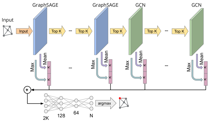
Node-level GNNs are used in this work because the values of interest, velocity and pressure, are defined at the nodes of the graph, and vertex selection is ultimately a node classification task. The DQN architecture used in this work is based on AirfoilGCNN, seen in figure 2, which is used for drag and lift prediction of airfoils in unstructured meshesOgoke_2021 . AirfoilGCNN makes use of GraphSAGEhamilton2017inductive and Graph ConvolutionalGCN layers as well as top-k poolingtopk . AirfoilGCNN has been modified for use in MeshDQN with an additional GraphSAGE layer, an additional GCN layer.
GraphSAGE layers are specifically designed to generate embeddings for unseen nodes, and are very well suited in this case where actions can result in a new vertex being added to the state space. Each GraphSAGE layer aggregates information from each vertex as well as its neighbors. In this work, aggregation is done as:
| (7) |
And the next state is given by:
| (8) |
Here, is the set of all neighbors of vertex , is a nonlinearity, and and are trainable weights in each layer.
GCN layers have been shown to perform well in node classification tasks, and so are also suitable choice here. GCN layers aggregate information in each layer, , through the adjacency matrix with self-self connection
| (9) |
where , is a trainable weight matrix in each layer, and is again a nonlinearity.
Top-K pooling is similar to max pooling, but selects the top-k fraction of data instead of the singular maximum value.
Skip connections are utilized in order to more effectively propagate information from each embedding into the final dense layers before classification. Our model was developed using Pytorch GeometricFey/Lenssen/2019 .
II.4 DRL Workflow
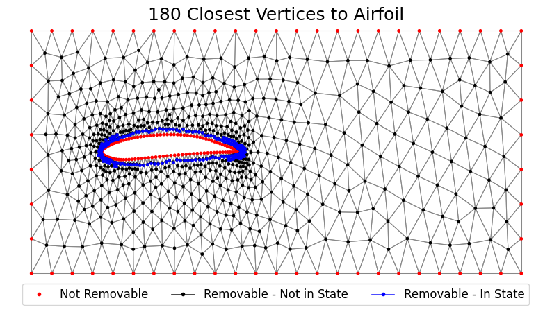
To begin our DRL training loop, we first run a simulation to calculate our target property using the IPCS scheme from section II.1. Our target property is then computed using the equation for either drag (Eq. 2) or lift (Eq. 3) and is our ground truth value . Intermediate and final solution states are stored as and , respectively, which will be referred to as snapshots. The number of snapshots to store can be tuned for the problem at hand. This is used to construct our initial state, which is stored as a graph, . Our state is defined as the closest vertices to the airfoil, seen in figure 3, inspired by an approach for designing nanoporesnanopore . Training was parallelized across 15 CPU cores using Ray, where 14 executed MeshDQN and the 15th acted as a server for DQN weights and updates.
II.4.1 State and Action Space
The node-level information at each vertex is:
Where is the and coordinates of each mesh vertex, is the and flow velocities at each vertex for each snapshot, is the pressure at each vertex for each snapshot, and indicates column-wise concatenation. The edge index is simply the connectivity between vertices in our mesh and the edge attribute is the Euclidean distance between vertices. The complete state space is given by which is a mixed continuous and discrete state space. Our action space is all vertices in the current state, as well as an additional ’no removal’ option that replaces the vertex nearest to the airfoil in the current state with the vertex nearest to the airfoil that is farther than all points in the current state. The ’no removal’ action stacks for a given episode, meaning that if the ’no removal’ action is selected times, then for a state consisting of 200 vertices, the vertices are the th through th closest to the airfoil.
Before initialization and after each vertex removal, the mesh is smoothed with local averaging 50 times for approximate convergence. Smoothing until convergence allows the full effect of each vertex removal to be realized immediately. This helps decorrelate actions from each other, making the dynamics of the system simpler.
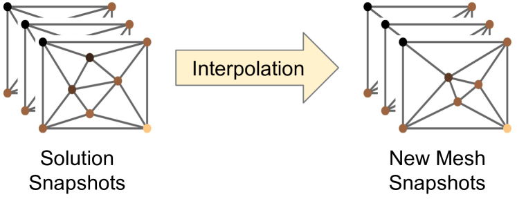
II.4.2 Interpolation
After vertex removal and smoothing is complete, the original snapshot values are interpolated onto the new mesh. Interpolation is done using piecewise elements as supported by FEniCS. Second order interpolation is done for velocities and first order is done for pressures. This matches the element order of the finite element method used in these simulations, which has shown acceptable accuracy. A toy example of interpolation is shown in figure 4.
II.4.3 Reward Function
Lastly, the reward function is defined in equation 10 where a broken mesh or broken interpolation returns a negative reward and ends the episode. The initial velocities and pressures are interpolated to the new mesh after each vertex removal and used for property estimation.
| (10) |
When the mesh and interpolation do not break, the reward is given by a property and time component, defined in equations 11 and 13, respectively. The factor is selected for an accuracy threshold of , in line with thresholds found in literatureullah_cfd_2021 . An error of yields a property reward of 0, and negative reward for worse accuracy. When the accuracy threshold is exceeded after a vertex removal, the episode is ended. Additionally, after a specified target number of vertices are removed the episode is ended. This reward incentivizes the selection of vertices that reduce error the smallest amount, and begins to penalize vertices if their removal results in too large of a drop in accuracy. The maximum property reward is 1, and the minimum is -1. A more in-depth exploration of the property reward function is given in Appendix A.
| (11) |
The factor can then be computed analytically by setting for an error of 0.0005 and solving for :
| (12) |
For the time reward, the factor is chosen so that the reward remains approximately constant after the removal of a vertex that results in a small, expected, drop in accuracy. This incentivizes vertex removals, and without this, MeshDQN would be rewarded for selecting ’no removal’ at every step. The full workflow is given in figure 1.
| (13) |
III Results
III.1 Mesh Improvement
Drag, specifically is used as the target property in these experiments. The YS930t_wing_1981 and AH93W145ah93w145 airfoils from the UIUC Airfoil Databaseselig_uiuc_1996 were used, with results in table 1. We use an accuracy threshold of 0.1%ullah_cfd_2021 and aim for 5% of vertices to be removed.
| Airfoil | Vertices Removed | Drag Error | Lift Error |
|---|---|---|---|
| YS930 | 5.023% | 0.039% | 0.002% |
| AH93W145 | 5.019% | 0.026% | 1.782% |
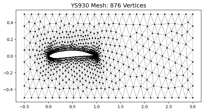
We see in figure 5 that MeshDQN is able to improve upon the selected airfoil, maintaining accuracy in the target property of drag for 44 vertices removed for the YS930 airfoil. This accuracy is maintained past a mesh that was generated using Delaunay triangulation and smoothing. Drag is also approximately maintained after each vertex removal, indicating MeshDQN is selecting vertices that maintain the drag at each step. The initial and final YS930 airfoils are give in figure 7. Plots for the AH93W145 airfoil are given in Appendix B.
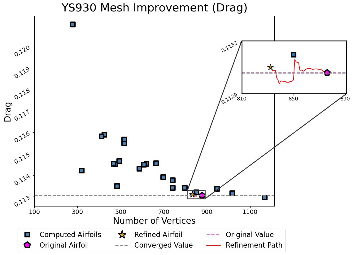
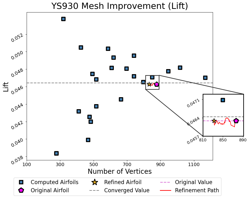
The initial and final meshes are given in figure 7. We see the mesh is sparser at the top and bottom surfaces of the airfoil, in the boundary flow layer where the flow is relatively simple.
a)
 b)
b)

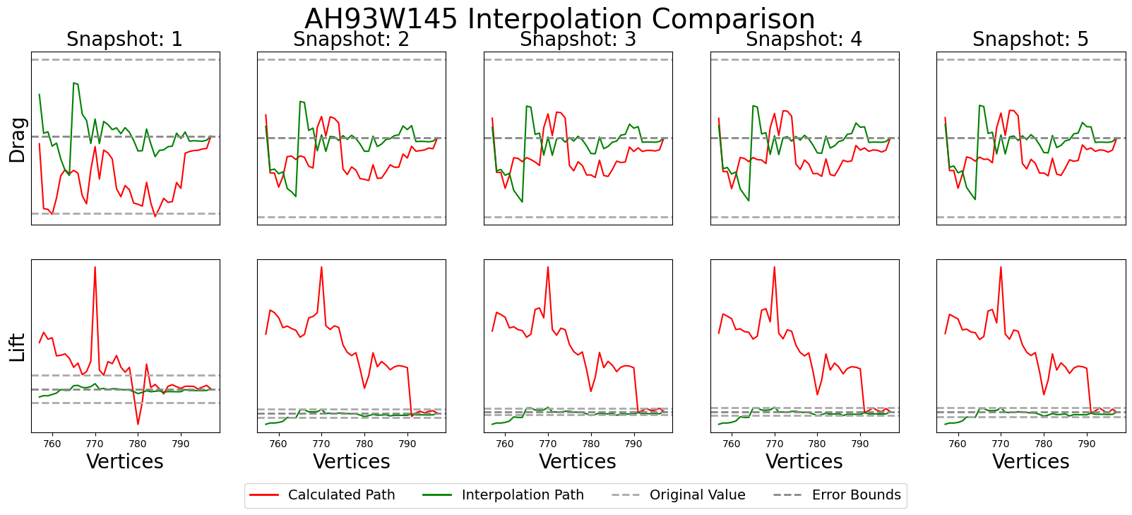
III.2 Interpolation Analysis
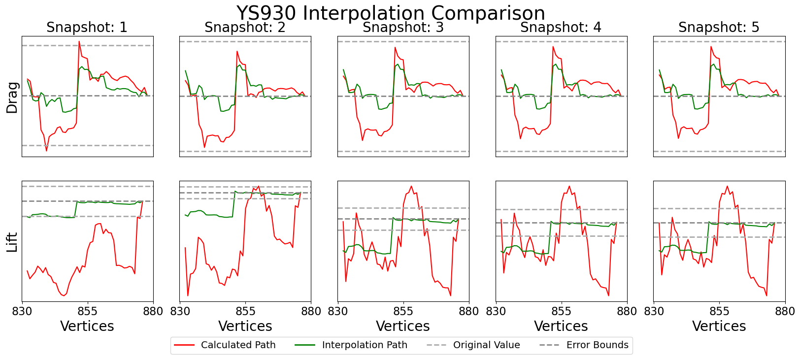
Interpolation is the key in allowing MeshDQN to quickly estimate target property values, and is of critical importance for accurate mesh improvement trajectories. Interpolated and calculated values are compared in figure 8. The green trajectory is the interpolated drag and lift value after each vertex removal, and the red trajectory is the value calculated from a full numerical simulation. In both figures, we see that the interpolated and calculated values correlate well with each other, generally showing shifts up and down in the same locations. However, the magnitude of shift is not the same. For lift, which was not used in training, there is little correlation between interpolated and calculated values.
IV Conclusion
We see MeshDQN has successfully taken fine meshes and selectively removed vertices while maintaining target property accuracy for 2D viscous, laminar flow for an unstructured mesh. MeshDQN is able to improve the mesh for multiple airfoils, while making no assumptions about the solver scheme, mesh type, flow regime, or dimensionality. While the current framework has demonstrated success at the given task, improved interpolation accuracy is of critical importance and is the current accuracy bottleneck.
While this work demonstrates a promising first step towards applying adaptive meshing to systems in CFD, there are many additional areas of CFD and meshing to explore. A promising future direction of research would be to apply this framework to new mesh types, such as structured, block structured, and arbitrary polygon unstructured meshes. Additionally, this work focused primarily on laminar flows, so applying this framework for turbulent flows remains an open problem. Further, this framework could be adapted to 3D geometries. Lastly, this framework was used simply for reducing the number of nodes in a fine mesh. In order to fully adapt a mesh to a particular problem, adding vertices to the mesh is necessary for refinement in regions of complex flow with high Reynolds number. This would also allow practitioners to begin with a relatively coarse mesh easy to generate mesh and adaptively refine the mesh to a given problem, making the CFD development significantly easier.
Author Contributions
Cooper Lorsung: conceptualization (equal); data curation, formal analysis; methodology (lead); software; validation (supporting); visualization; writing - original draft preparation; writing - review and editing (lead)
Amir Barati Farimani: conceptualization (equal); resources; methodology (supporting); resources; validation (supporting); supervision; writing - review and editing (supporting)
Acknowledgements
CL acknowledges Francis Ogoke for providing starter simulation code and helping with debugging. CL acknowledges Zhonglin Cao for the idea of using closest vertices to the airfoil.
This material is based upon work supported by the National Science Fountation under Grant No. 1953222
Author Declaration
The authors have no conflicts to disclose.
Data Availability
MeshDQN code and data are available at: https://github.com/BaratiLab/MeshDQN
Appendix A Reward Function Design
Reward function design is a critical component of the MeshDQN framework. Selecting a good value, as in equation 11, determines how strongly a vertex removal with high error, and in turn, allows MeshDQN to distinguish between low and high error vertex removals. Selecting too small of a value leads to rewards that are too close together to reliably learn which vertex removals lead to low and high error. On the other hand, selecting too large of a value causes issues in the other direction, where too many vertex removals are penalized, even with fairly small error. Selecting a proper value is therefore a balancing act.
As mentioned in section II.4.3, intuition guides us to select based on where we have reward. This allows us to set an penalty threshold, above which we penalize vertex removals, and below which we incentivize them. We see in figure 9 three different options. We can set 0 reward at the total error threshold, halfway to the error threshold, or a quarter of the way to the error threshold. Empirically, we have found setting the penalty threshold halfway to the way to the error threshold works well, leading to a variety of actions selected. Setting the penalty threshold higher does not generally provide a strong enough penalty for MeshDQN to reliably distinguish between actions, often times leading to mode collapse and a single action being selected repeatedly. Setting the threshold lower often leads to all removals being penalized too strongly, and MeshDQN learns to only select ’no removal’.

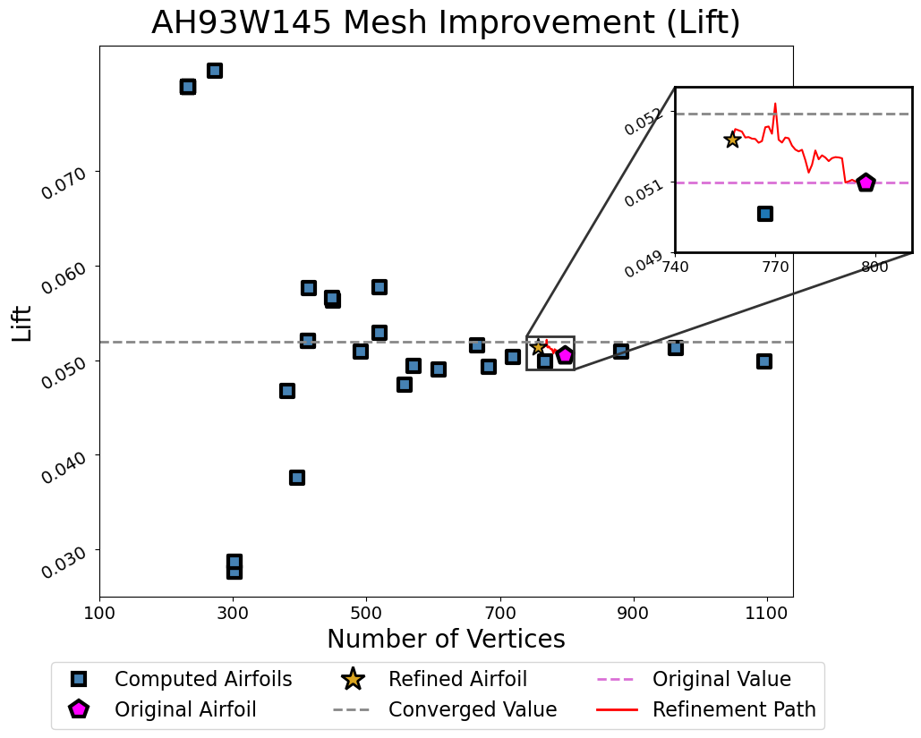
Appendix B AH93W145 Analysis
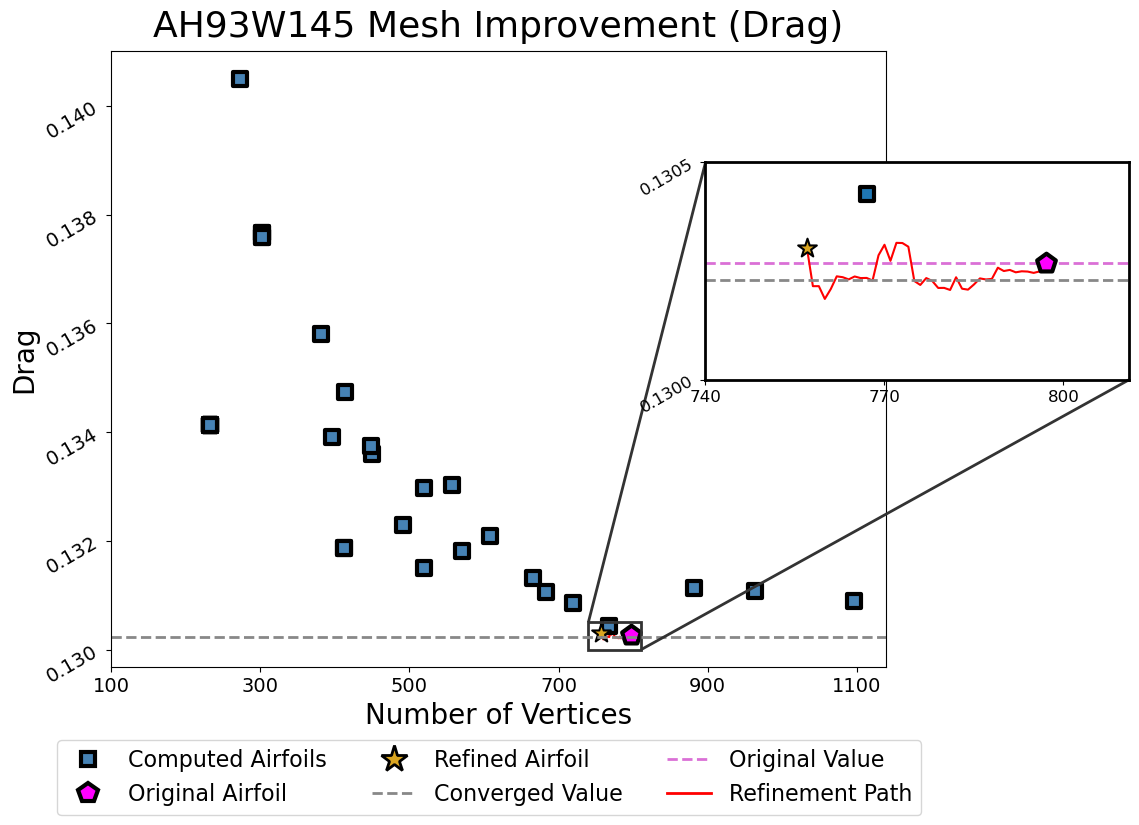
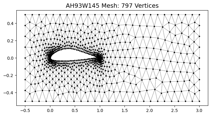
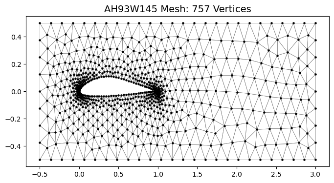
Further analysis of the AH93W145 airfoil is given here. We have the drag improvement in figure 10, where we see the drag is improved past a generated meshing. Lift improvement is given in figure 11, where we see the calculated lift value is not maintained as well, but still remains well within the region of other generated meshes. The initial and final meshes are given in figure 12, where we see the mesh at the top and bottom faces of the airfoil have been slightly coarsened.
a)
 b)
b)
Appendix C Simulation and Training Configuration
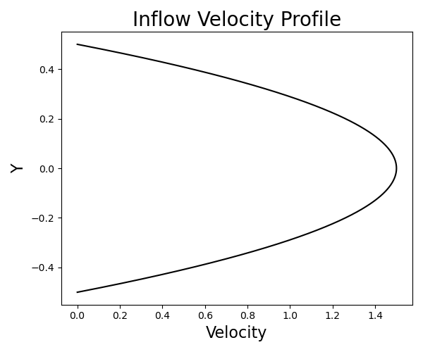
The flow solver was configured with no-slip boundary conditions on the airfoil, top and bottom walls. Zero pressure was used at the outlet. The inflow velocity profile is constant with respect to time and given in figure 14.
The simulation was done with unitless equations. Viscosity was set to 0.001, with density of 1, which gives us a Reynolds number of 1800. The timestep was set to 0.001, for 5000 timesteps, for a total of a five second simulation. The discount factor was set to 1. The Adam optimizerDBLP:journals/corr/KingmaB14 was used with a learning rate of 0.0005 and no weight decay. The weights and biases of each layer were initialized with Xavier normal initializerpmlr-v9-glorot10a using a gain of 0.9. A convolutional width of 128 was used for each GraphSAGE and GCN layer. Two GraphSAGE and GCN layers were used. Additionally, training was parallelized using Ray. Five evenly spaces snapshots were used at timestep 1000, 2000, 3000, 4000, and 5000.
References
References
- (1) Slotnick J., Khodadoust A., Alonso J., Darmofal D., Gropp W., Lurie E., Mavriplis D. “CFD Vision 2030 Study: A Path to Revolutionary Computational Aerosciences.” p. 58, 2014
- (2) Baker T.J. “Mesh generation: Art or science?” Progress in Aerospace Sciences, vol. 41, no. 1, 29–63, 2005. URL https://www.sciencedirect.com/science/article/pii/S0376042105000114
- (3) Chawner J.R., Taylor N.J. “Progress in Geometry Modeling and Mesh Generation Toward the CFD Vision 2030.” AIAA Aviation 2019 Forum. American Institute of Aeronautics and Astronautics, Dallas, Texas, Jun. 2019. URL https://arc.aiaa.org/doi/10.2514/6.2019-2945
- (4) Park M.A., Loseille A., Krakos J., Michal T.R., Alonso J.J. “Unstructured Grid Adaptation: Status, Potential Impacts, and Recommended Investments Towards CFD 2 030.” 46th AIAA Fluid Dynamics Conference, AIAA AVIATION Forum. American Institute of Aeronautics and Astronautics, Jun. 2016. URL https://arc.aiaa.org/doi/10.2514/6.2016-3323
- (5) Alauzet F., Loseille A. “A decade of progress on anisotropic mesh adaptation for computational fluid dynamics.” Computer-Aided Design, vol. 72, 13–39, 2016. URL https://www.sciencedirect.com/science/article/pii/S0010448515001517. 23rd International Meshing Roundtable Special Issue: Advances in Mesh Generation
- (6) Huang K., Krügener M., Brown A., Menhorn F., Bungartz H.J., Hartmann D. “Machine Learning-Based Optimal Mesh Generation in Computational Fluid Dynamics.”, 2021. URL https://arxiv.org/abs/2102.12923
- (7) Xu H., Nie Z., Xu Q., Li Y., Xie F., Liu X.J. “SuperMeshing: Boosting the Mesh Density of Stress Field in Plane Strain Problems using Deep Learning Method.” Journal of Computing and Information Science in Engineering, pp. 1–12, 05 2022. URL https://doi.org/10.1115/1.4054687
- (8) Garnier P., Viquerat J., Rabault J., Larcher A., Kuhnle A., Hachem E. “A review on Deep Reinforcement Learning for Fluid Mechanics.”, 2019. URL https://arxiv.org/abs/1908.04127
- (9) Viquerat J., Meliga P., Hachem E. “A review on deep reinforcement learning for fluid mechanics: an update.”, 2021. URL https://arxiv.org/abs/2107.12206
- (10) Li Z., Meidani K., Farimani A.B. “Transformer for Partial Differential Equations’ Operator Learning.”, 2022. URL https://arxiv.org/abs/2205.13671
- (11) “Graph neural network-accelerated Lagrangian fluid simulation.” vol. 103. URL https://www.sciencedirect.com/science/article/pii/S0097849322000206
- (12) Pant P., Doshi R., Bahl P., Barati Farimani A. “Deep learning for reduced order modelling and efficient temporal evolution of fluid simulations.” Physics of Fluids, vol. 33, no. 10, 107101, Oct. 2021. URL https://aip.scitation.org/doi/abs/10.1063/5.0062546. Publisher: American Institute of Physics
- (13) Jiang C., Farimani A.B. “Deep Learning Convective Flow Using Conditional Generative Adversarial Networks.”, 2020. URL https://arxiv.org/abs/2005.06422
- (14) Meidani K., Barati Farimani A. “Data-driven identification of 2D Partial Differential Equations using extracted physical features.” Computer Methods in Applied Mechanics and Engineering, vol. 381, 113831, Aug. 2021. URL https://www.sciencedirect.com/science/article/pii/S0045782521001687
- (15) Barber C.B., Dobkin D.P., Huhdanpaa H. “The Quickhull algorithm for convex hulls.” ACM TRANSACTIONS ON MATHEMATICAL SOFTWARE, vol. 22, no. 4, 469–483, 1996
- (16) Geuzaine C., Remacle J.F. “Gmsh: a three-dimensional finite element mesh generator with built-in pre- and post-processing facilities.” International Journal for Numerical Methods in Engineering, vol. 79, 1309–1331, 2009
- (17) Schlömer N., nilswagner, Li T., Coutinho C., Dalcin L., McBain G., Cervone A., Langlois T., Peak S., Bussonnier M., lgiraldi, Vaillant G.A., Croucher A. “nschloe/meshio v1.11.7.”, Feb. 2018. URL https://doi.org/10.5281/zenodo.1173116
- (18) Goda K. “A multistep technique with implicit difference schemes for calculating two- or three-dimensional cavity flows.” Journal of Computational Physics, vol. 30, no. 1, 76–95, Jan. 1979. URL https://www.sciencedirect.com/science/article/pii/0021999179900883
- (19) A. Logg G.N.W., Hake J. “DOLFIN: a C++/Python Finite Element Library.” K.M. A. Logg, G.N. Wells, editors, Automated Solution of Differential Equations by the Finite Element Method, vol. 84 of Lecture Notes in Computational Science and Engineering, chap. 10. Springer, 2012
- (20) Logg A., Wells G.N. “DOLFIN: Automated Finite Element Computing.” ACM Transactions on Mathematical Software, vol. 37, 2010
- (21) Langtangen H.P., Logg A. “Solving PDEs in Python – The FEniCS Tutorial Volume I.” p. 153
- (22) van Hasselt H., Guez A., Silver D. “Deep Reinforcement Learning with Double Q-learning.”, 2015. URL https://arxiv.org/abs/1509.06461
- (23) Wu Z., Pan S., Chen F., Long G., Zhang C., Yu P.S. “A Comprehensive Survey on Graph Neural Networks.” IEEE Transactions on Neural Networks and Learning Systems, vol. 32, no. 1, 4–24, 2021
- (24) Ogoke F., Meidani K., Hashemi A., Farimani A.B. “Graph convolutional networks applied to unstructured flow field data.” Machine Learning: Science and Technology, vol. 2, no. 4, 045020, sep 2021. URL https://doi.org/10.1088/2632-2153/ac1fc9
- (25) Hamilton W.L., Ying R., Leskovec J. “Inductive Representation Learning on Large Graphs.” NIPS. 2017
- (26) Kipf T.N., Welling M. “Semi-Supervised Classification with Graph Convolutional Networks.”, 2016. URL https://arxiv.org/abs/1609.02907
- (27) Cangea C., Veličković P., Jovanović N., Kipf T., Liò P. “Towards Sparse Hierarchical Graph Classifiers.”, 2018. URL https://arxiv.org/abs/1811.01287
- (28) Fey M., Lenssen J.E. “Fast Graph Representation Learning with PyTorch Geometric.” ICLR Workshop on Representation Learning on Graphs and Manifolds. 2019
- (29) Wang Y., Cao Z., Barati Farimani A. “Efficient water desalination with graphene nanopores obtained using artificial intelligence.” npj 2D Materials and Applications, vol. 5, no. 1, 1–9, Jul. 2021. URL https://www.nature.com/articles/s41699-021-00246-9. Number: 1 Publisher: Nature Publishing Group
- (30) Ullah A., Zaman M.B., Bhatti M.A., Qasim D., Hamid A., Xiong Q., Khan A. “CFD study of drag and lift coefficients of non-spherical particles.” Journal of King Saud University - Engineering Sciences, 2021. URL https://www.sciencedirect.com/science/article/pii/S1018363921001422
- (31) T S.Y., R E. “Wing sections for hydrofoils - Part 2: Nonsymmetrical profiles.” Journal of Ship Research, vol. 25, no. 3, 191–200, 1981. URL https://jglobal.jst.go.jp/en/detail?JGLOBAL_ID=200902072484484263
- (32) Althaus D. Niedriggeschwindigkeitsprofil. Vieweg, 1996
- (33) Selig M.S. UIUC airfoil data site. Urbana, Ill. : Department of Aeronautical and Astronautical Engineering Univ ersity of Illinois at Urbana-Champaign, 1996-, 1996. URL https://search.library.wisc.edu/catalog/999919007002121
- (34) Kingma D.P., Ba J. “Adam: A Method for Stochastic Optimization.” ICLR (Poster). 2015. URL http://arxiv.org/abs/1412.6980
- (35) Glorot X., Bengio Y. “Understanding the difficulty of training deep feedforward neural networks.” Y.W. Teh, M. Titterington, editors, Proceedings of the Thirteenth International Conference on Artificial Intelligence and Statistics, vol. 9 of Proceedings of Machine Learning Research, pp. 249–256. PMLR, Chia Laguna Resort, Sardinia, Italy, 13–15 May 2010. URL https://proceedings.mlr.press/v9/glorot10a.html