Isovector Axial Form Factor of the Nucleon
from Lattice QCD

Abstract

The isovector axial form factor of the nucleon plays a key role in interpreting data from long-baseline neutrino oscillation experiments. We present a lattice QCD calculation of this form factor, introducing a new method to directly extract its $z$-expansion from lattice correlators. Our final parameterization of the form factor, which extends up to spacelike virtualities of $0.7\,{\rm GeV}^{2}$ with fully quantified uncertainties, agrees with previous lattice calculations but is significantly less steep than neutrino-deuterium scattering data suggests.

1 Motivation

The axial form factor of the nucleon $G_{\rm A}(Q^{2})$ plays a central role in understanding the quasi-elastic part of GeV-scale neutrino-nucleus cross sections. These cross sections must be known with few-percent uncertainties [1] to enable a reliable reconstruction of the incident neutrino energy in the upcoming long-baseline neutrino oscillation experiments DUNE [2] and T2HK [3]. Lattice QCD determinations of $G_{\rm A}(Q^{2})$ [4] are crucial, as currently available experimental measurements of the form factor fall short of the required precision [5].

Here we summarize the Mainz group’s recent calculation of $G_{\rm A}(Q^{2})$ [6] for momentum transfers up to $0.7\,{\rm GeV}^{2}$ using lattice simulations with dynamical up, down and strange quarks with an O($a$) improved Wilson fermion action. We employ a new analysis method that simultaneously handles the issues of the excited-state contamination and the description of the form factor’s $Q^{2}$ dependence.

2 Methodology

The matrix elements of the local isovector axial current $A^{a}_{\mu}(x)=\bar{\psi}\gamma_{\mu}\gamma_{5}\frac{\tau^{a}}{2}\psi$ between single-nucleon states are parameterized by two form factors: the axial form factor $G_{\rm A}(Q^{2})$, and the induced pseudoscalar form factor $G_{\rm P}(Q^{2})$. We focus on calculating the axial form factor, which can be extracted from the current component orthogonal to the momentum transfer.

The setup for the lattice calculation in this project [6] is very similar to the one used in the case of the electromagnetic form factors [7]. The nucleon two- and three-point functions are computed as

$$C_{2}(\vec{p},t)= a^{3}\sum_{\vec{x}}e^{i\vec{p}\cdot\vec{x}}\Gamma_{\beta\alpha}\Big{\langle}\Psi^{\alpha}(t,\vec{x})\overline{\Psi}^{\beta}(0)\Big{\rangle},$$ (1)

$$C_{3}(\vec{q},t,t_{s})= -ia^{6}\sum_{\vec{x},\vec{y}}e^{i\vec{q}\cdot\vec{y}}\Gamma_{\beta\alpha}\frac{\vec{q}\times\vec{s}}{|\vec{q}\times\vec{s}|^{2}}\Big{\langle}\Psi^{\alpha}(t_{s},\vec{x})\vec{q}\times\vec{A}^{a=3}(t,\vec{y})\overline{\Psi}^{\beta}(0)\Big{\rangle},$$

where $t_{s}$ is the source-sink separation in the time direction, $\Psi^{\alpha}(\vec{x},t)$ denotes the proton interpolating operator and $\Gamma=\frac{1}{2}(1+\gamma_{0})(1+i\gamma_{5}\vec{s}\cdot\vec{\gamma})$ is the projection matrix. We set $\vec{s}=\vec{e}_{3}$, aligning the nucleon spin along the $x_{3}$-axis.

2.1 Summation method + $z$-expansion

The accessible momentum transfers are discrete, and for a given value of $\mathfrak{q}={2\pi|\vec{n}|}/{L}$, we perform averages of the two-point functions over all spatial momenta $\vec{q}$ of the same norm $\mathfrak{q}$. We then use the ratio

$$R(\vec{q},t,t_{s})\equiv\frac{C_{3}(\vec{q},t,t_{s})}{\overline{C}_{2}(0,t_{s})}\sqrt{\frac{\overline{C}_{2}(|\vec{q}|,t_{s}-t)\overline{C}_{2}(0,t)\overline{C}_{2}(0,t_{s})}{\overline{C}_{2}(0,t_{s}-t)\overline{C}_{2}(|\vec{q}|,t)\overline{C}_{2}(|\vec{q}|,t_{s})}}$$ (2)

to construct a momentum-averaged estimator for $G_{\rm A}(Q^{2})$,

$$G^{\rm eff}_{\rm A}(\mathfrak{q};t,t_{s})=\sqrt{\frac{2E_{\mathfrak{q}}}{m+E_{\mathfrak{q}}}}\sum_{|\vec{q}|=\mathfrak{q}}R(\vec{q},t,t_{s})\Big{/}\Big{(}\sum_{|\vec{q}|=\mathfrak{q}}1\Big{)}.$$ (3)

Here $m$ is the nucleon mass and $E_{\mathfrak{q}}$ its energy. These effective form factors are then used to construct the summed insertion

$$S(\mathfrak{q},t_{s})\equiv a\sum_{t=a}^{t_{s}-a}G^{\rm eff}_{\rm A}(\mathfrak{q};t,t_{s})\stackrel{{\scriptstyle t_{s}\to\infty}}{{=}}b_{0}(\mathfrak{q})+t_{s}G_{\rm A}(Q^{2})+\dots$$ (4)

with momentum transfer $Q^{2}=\mathfrak{q}^{2}-(m-E_{\mathfrak{q}})^{2}$. The excited states, indicated by the ellipsis, are of order $e^{-\Delta t_{s}}$ and $t_{s}e^{-\Delta t_{s}}$, with $\Delta$ the energy gap above the single-nucleon state.

To extract the form factor $G_{\rm A}(Q^{2})$, we parametrize it from the outset via the $z$-expansion

$$G_{\rm A}(Q^{2})=\sum^{n_{\rm max}}_{n=0}a_{n}z^{n}(Q^{2}),\quad z(Q^{2})=\frac{\sqrt{t_{\rm cut}+Q^{2}}-\sqrt{t_{\rm cut}}}{\sqrt{t_{\rm cut}+Q^{2}}+\sqrt{t_{\rm cut}}},$$ (5)

fitting simultaneously the $\mathfrak{q}$ and $t_{s}$ dependence of $S(\mathfrak{q},t_{s})$. Here $t_{\rm cut}=(3M_{\pi}^{\rm phys})^{2}$, and both the offsets $b_{0}(\mathfrak{q})$ (independent for each $\mathfrak{q}$) and the coefficients $a_{n}$ are fit parameters. We set $n_{\rm max}=2$ in our main analysis, and test that setting $n_{\rm max}=3$ gives consistent results. In the future, we will also consider parametrizing the $\mathfrak{q}$ dependence of $b_{0}(\mathfrak{q})$.

2.2 Choice of source-sink separation

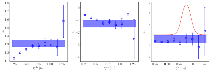
Figure 1: Illustration of averaging over the minimum source-sink separation $t_{s}^{\mathrm{min}}$ in the summation method for the near-physical pion mass ensemble E250. We perform the $z$-expansion fits for each ensemble starting at different values of $t_{s}^{\mathrm{min}}$. The results for coefficients $a_{0}$, $a_{1}$ and $a_{2}$ are shown here as the blue squares. The bands represent the smooth-window averages over $t_{s}^{\mathrm{min}}$, and the solid red line shows the weight function (arbitrarily normalized for visibility), which is applied to all three coefficients.

We perform fits to $S(\mathfrak{q},t_{s})$ including all values of $t_{s}\geq t_{s}^{\textrm{min}}$, requiring that at least two $t_{s}$ values enter the fit (and also requiring $n_{\textrm{dof}}>0$). At small values of $t_{s}$, contributions from excited states are expected to be significant, whereas at large $t_{s}$ the signal-to-noise ratio becomes poor. This leaves us with a relatively small window of starting values $t_{s}^{\textrm{min}}$ that can be used. Rather than choosing a single $t_{s}^{\textrm{min}}$, we average the fit results $a_{n}(t_{s}^{\textrm{min}})$ over all values $t_{s}^{\textrm{min}}$, using a ‘smooth window’ function $f(t_{s}^{\textrm{min}})$,

$$a_{n}=\sum_{t_{s}^{\textrm{min}}}f(t_{s}^{\textrm{min}})a_{n}(t_{s}^{\textrm{min}})\Big{/}\Big{(}\sum_{t_{s}^{\textrm{min}}}f(t_{s}^{\textrm{min}})\Big{)},\quad f(\tau)=\tanh{\left(\frac{\tau-t_{w}^{\textrm{low}}}{\Delta t_{w}}\right)}-\tanh{\left(\frac{\tau-t_{w}^{\textrm{up}}}{\Delta t_{w}}\right)},$$ (6)

as a weight factor. We choose $t_{w}^{\textrm{low}}=0.8$ fm, $t_{w}^{\textrm{up}}=1.0$ fm and $\Delta t_{w}=0.08$ fm. The average represents very well what one would identify as a plateau in the fit results, as illustrated in Fig. 1.

3 Lattice ensembles

We use a set of fourteen CLS $N_{f}=2+1$ ensembles [8] that have been generated with non-perturbatively $\mathcal{O}(a)$-improved Wilson fermions [9, 10] and the tree-level improved Lüscher-Weisz gauge action [11]. They cover the range of lattice spacings from $0.050$ fm to $0.086$ fm and pion masses from about $350~{}\textrm{MeV}$ down to $130~{}\textrm{MeV}$. Details of these ensembles, including the number of configurations, the number of measurements and the number of available source-sink separations $t_{s}$, are listed in Table 1. All ensembles used in this study have a fairly large volume, as indicated by $M_{\pi}L\gtrsim 4$.

ID	$\beta$	$T/a$	$L/a$	$\!\!M_{\pi}/\textrm{MeV}$	$M_{\pi}L$	$\!\!M_{N}/\textrm{GeV}$	$N_{\mathrm{conf}}$	$N_{\mathrm{meas}}$	$t_{s}~{}[\textrm{fm}]$	$N_{t_{s}}$
H102	3.40	96	32	354	4.96	1.103	2005	32080	0.35..1.47	14
H105	3.40	96	32	280	3.93	1.045	1027	49296	0.35..1.47	14
C101	3.40	96	48	225	4.73	0.980	2000	64000	0.35..1.47	14
N101	3.40	128	48	281	5.91	1.030	1596	51072	0.35..1.47	14
S400	3.46	128	32	350	4.33	1.130	2873	45968	0.31..1.53	9
N451	3.46	128	48	286	5.31	1.045	1011	129408	0.31..1.53	9
D450	3.46	128	64	216	5.35	0.978	500	64000	0.31..1.53	17
N203	3.55	128	48	346	5.41	1.112	1543	24688	0.26..1.41	10
N200	3.55	128	48	281	4.39	1.063	1712	20544	0.26..1.41	10
D200	3.55	128	64	203	4.22	0.966	2000	64000	0.26..1.41	10
E250	3.55	192	96	129	4.04	0.928	400	102400	0.26..1.41	10
N302	3.70	128	48	348	4.22	1.146	2201	35216	0.20..1.40	13
J303	3.70	192	64	260	4.19	1.048	1073	17168	0.20..1.40	13
E300	3.70	192	96	174	4.21	0.962	570	18240	0.20..1.40	13

Table 1: Overview of ensembles used in the study. The values $\beta=3.40$, $3.46$, $3.55$ and $3.70$ correspond to lattice spacings $a\approx 0.086$, $0.076$, $0.064$ and $0.050~{}\textrm{fm}$, respectively [12]. Columns $T/a$ and $L/a$ give the temporal and spatial size of the lattice, and $M_{\pi}$ and $M_{N}$ are the pion and nucleon masses. $N_{\mathrm{conf}}$ is the number of configurations used for each ensemble, and in column $N_{\mathrm{meas}}$ we list the number of measurements done at the largest source-sink separation. $N_{t_{s}}$ is the number of available source-sink separations in the range listed in column $t_{s}$. For more details see [6].

4 Global fit

To obtain the form factor at the physical point, the $a_{n}$ are extrapolated to the continuum and interpolated to the physical pion mass, at which point the form factor may be evaluated at any $q^{2}$ in the chosen expansion interval $[0,\;0.7\,{\rm GeV}^{2}]$.

For the extrapolation to the continuum, we include a term linear in $a^{2}$ for each of the coefficients. For the extrapolation in pion mass, we use the following three ansätze:

1. Linear in $M_{\pi}^{2}$ for all coefficients $a_{n}$.

2. Again linear in $M_{\pi}^{2}$ for coefficients $a_{1}$ and $a_{2}$, and an extended ansatz containing a chiral logarithm for the zeroth coefficient:

   $$a_{0}=g_{a}^{(0)}+g_{a}^{(1)}M_{\pi}^{2}+g_{a}^{(3)}M_{\pi}^{3}-g_{a}^{(2)}M_{\pi}^{2}\ln{\frac{M_{\pi}}{M_{N}}},$$

   with $g_{a}^{(1)}=4d_{16}-(g_{a}^{(0)})^{3}/(16\pi^{2}F_{\pi}^{2}$, $g_{a}^{(2)}=g_{a}^{(0)}\left(1+2(g_{a}^{(0)})^{2}\right)/(8\pi^{2}F_{\pi}^{2})$, and $g_{a}^{(3)}=g_{a}^{(0)}\left(1+(g_{a}^{(0)})^{2}\right)/(8\pi F_{\pi}^{2}M_{N})-g_{a}^{(0)}\Delta_{c_{3},c_{4}}/(6\pi F_{\pi}^{2})$. Here $M_{N}=938.92~{}\textrm{MeV}$ is the nucleon mass, $F_{\pi}=92.42~{}\textrm{MeV}$ is the pion decay constant [13], and $\Delta_{c_{3},c_{4}}=c_{3}-2c_{4}$ is a combination of low-energy constants $c_{3}$ and $c_{4}$. The free fit parameters for the zeroth coefficient’s chiral extrapolation are $g_{a}^{(0)}$, $d_{16}$ and $\Delta_{c_{3},c_{4}}$.

3. Same as ansatz 2, but including $M_{\pi}^{3}$ terms for coefficients $a_{1}$ and $a_{2}$.

Note that, while the coefficients $a_{n}$ do not have common fit parameters, they are correlated within an ensemble: these correlations are taken into account in the fits.

To check for possible finite-size effects (FSE), we include a term [14] $\frac{M_{\pi}^{2}}{\sqrt{M_{\pi}L}}\mathrm{e}^{-M_{\pi}L}$ for the zeroth coefficient $a_{0}$ in some of the extrapolation fits. We do not observe a strong dependence on the volume. Finite-size effects can also be inspected directly by comparing our results of the $z$-expansion fits on two ensembles, H105 and N101, which differ only by their physical volume. We find that the coefficients $a_{n}$ agree well, confirming that finite-size effects are small at the current level of precision.

We perform multiple extrapolations using these different fit ansätze with pion mass cuts $M_{\pi}<M_{\pi}^{\rm cut}$ with $M_{\pi}^{\rm cut}=$ 300, 285, 265 and 250 MeV, as well as dropping data from the coarsest lattice spacing, to get a handle on systematic effects.

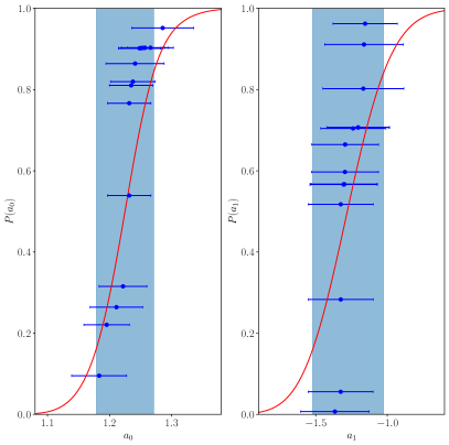
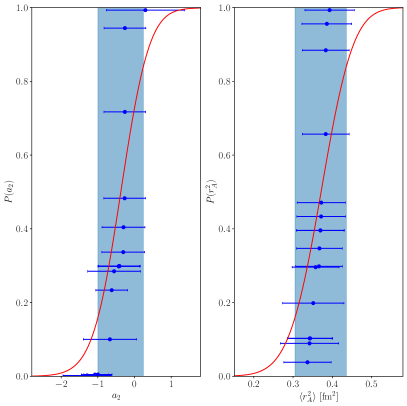
Figure 2: AIC average and the corresponding cumulative distribution function for all coefficients $a_{0}$, $a_{1}$, $a_{2}$, and the mean square radius $\langle r_{A}^{2}\rangle$ (in fm² units).

5 Model average (AIC)

Since the different fit ansätze and cuts can be equally well motivated, we perform a weighted average [15] over the resulting $a_{n}$. The Akaike Information Criterion (AIC) [16] is used to provide the weight to different analyses and to estimate the systematic error associated with the variations of the global fit. Different variations of the AIC weights have been used over the years, and we choose [17] $w^{\textrm{AIC}}=N\mathrm{e}^{-\frac{1}{2}\left(\chi^{2}+2n_{\textrm{par}}-n_{\textrm{data}}\right)}$, where each fit is characterized by the minimum $\chi^{2}$, the number of fit parameters $n_{\textrm{par}}$ and the number of data points $n_{\textrm{data}}$. Here $N$ normalizes the weights so that their sum is 1.

The corresponding cumulative distribution functions $P(a_{n})$ of the coefficients $a_{n}$ and of the mean square radius $\langle r_{A}^{2}\rangle$ are shown in Fig. 2. The full uncertainties, which are shown by the blue error bands, are determined by the limits $P(a_{n})=0.16$ and $P(a_{n})=0.84$. The AIC procedure is also used to distinguish the statistical and systematic components of the total uncertainty, following the prescription proposed in [17].

6 Results

Our results for the coefficients of the $z$-expansion (Eq. (5) with $t_{\rm cut}=(3M_{\pi^{0}})^{2}$) of the nucleon axial form factor in the continuum and at the physical pion mass are

$$a_{0}= \quad\>1.225\pm 0.039\textrm{ (stat)}\pm 0.025\textrm{ (syst)},$$

$$a_{1}= -1.274\pm 0.237\textrm{ (stat)}\pm 0.070\textrm{ (syst)},$$ (7)

$$a_{2}= -0.379\pm 0.592\textrm{ (stat)}\pm 0.179\textrm{ (syst)},$$

with a correlation matrix

$$M_{\textrm{corr}}=\left(\!\begin{array}[]{rrr}1.00000&-0.67758&0.61681\\ -0.67758&1.00000&-0.91219\\ 0.61681&-0.91219&1.00000\end{array}\,\right).$$ (8)

This leads to the mean square radius $\langle r^{2}_{A}\rangle=(0.370\pm 0.063\textrm{ (stat)}\pm 0.016\textrm{ (syst)})~{}\textrm{fm}^{2}$, which is in good agreement with other lattice QCD determinations – see Fig. 3. The comparison features only lattice calculations with a full error budget, including a continuum extrapolation: The NME21 result is from [18], and the RQCD20 result is from [19]. Both studies parameterize the $Q^{2}$ dependence of the form factor using a $z$-expansion (RQCD also use a dipole ansatz as an alternative parameterization, the result of which is not shown in the figure). Other lattice calculations [20, 21, 22, 23, 24] also exist with partial error budgets. For comparison, we show the average of the values obtained from $z$-expansion fits to neutrino scattering and muon capture measurements [25]. Our result also agrees well with the earlier two-flavour calculation by the Mainz group [26], and with a more recent analysis [27] by the same group that has been obtained via the conventional two-step process of first determining the form factor at discrete $Q^{2}$ values and then parameterizing it using a $z$-expansion.

The axial charge $g_{A}=a_{0}$ is in good agreement with our previous determination [28] based on forward nucleon matrix elements only. Since that method tends to yield more precise results for a given data set, we do not view the present determination of $g_{A}$ as superseding that of Ref. [28], and merely perform the comparison as a consistency check.

Finally, we compare our result for the axial form factor to data from pion electroproduction experiments [5] and to a $z$-expansion fit to neutrino-Deuterium scattering data [29] in Fig. 3. Our result agrees well with other lattice QCD calculations, as can be seen by comparing this figure to Fig. 3 in the recent review [4]. However, there is a tension with the axial form factor extracted from experimental deuterium bubble chamber data [29], especially at large $Q^{2}$. According to the authors of the Snowmass White Paper on Neutrino Scattering Measurements [30], this discrepancy suggests that a 30-40% increase would be needed in the nucleon quasielastic cross section for the two results to match. They also note that recent high-statistics data on nuclear targets cannot directly resolve such discrepancies due to nuclear modeling uncertainties.

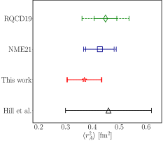
(a)

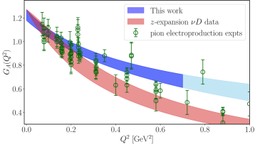
(b)

Figure 3: (a): Comparison of lattice determinations of the mean square radius $\langle r_{\text{A}}^{2}\rangle$, from Refs. [18] (NME21) and [19] (RQCD20), which have full error budget (chiral and continuum extrapolation). The point labeled Hill et al. is an average of the values obtained from $z$-expansion fits to neutrino scattering and muon capture [25]. The smaller error bars with solid lines show the statistical errors, whereas the wider error bars with dashed lines show the total errors (including systematic uncertainties). (b): Comparing our result for the axial form factor to data from pion electroproduction experiments [5] (normalized by the PDG value for the axial charge [31]) and to a $z$-expansion fit to neutrino-Deuterium scattering data [29]. There is a clear tension between the lattice QCD result and the $z$-expansion extracted from deuterium bubble chamber data, especially at large $Q^{2}$. The darker blue error band highlights the $Q^{2}$ range of our lattice data.

7 Summary and conclusions

In this report, we have given a summary of the Mainz group’s recent publication [6], which introduced a new method to extract the axial form factor of the nucleon. It combines two well-known methods into one analysis step: the summation method, which ensures that excited-state effects are sufficiently suppressed, and the $z$-expansion, which provides the parameterization of the $Q^{2}$ dependence of the form factor. Our main results are the coefficients of the $z$-expansion, given in Eq. (7). Systematic effects are included through AIC weighted average, which also provides the break-up into statistical and systematic uncertainties and the correlations among the coefficients.

We observe good agreement with other lattice QCD determinations of the axial form factor, which confirms and strengthens the tension with the shape of the form factor extracted from deuterium bubble chamber data. Comparing our result for $a_{0}\equiv G_{\rm A}(0)$ to the Particle Data Group (PDG) value for the axial charge, $g_{A}=1.2754(13)$ [31], which can be viewed as a benchmark, we find agreement at the $1.1\,\sigma$ level. Also, previously, a good overall agreement was found for the isovector vector form factors [7] with phenomenological determinations, which are far more precise than in the axial-vector case. This all adds confidence to the finding that the nucleon axial form factor falls off less steeply than previously thought.

References

- [1] L.A. Ruso et al., Theoretical tools for neutrino scattering: interplay between lattice QCD, EFTs, nuclear physics, phenomenology, and neutrino event generators, 2203.09030.
- [2] DUNE collaboration, Long-Baseline Neutrino Facility (LBNF) and Deep Underground Neutrino Experiment (DUNE): Conceptual Design Report, Volume 2: The Physics Program for DUNE at LBNF, 1512.06148.
- [3] Hyper-Kamiokande collaboration, Hyper-Kamiokande Design Report, 1805.04163.
- [4] A.S. Meyer, A. Walker-Loud and C. Wilkinson, Status of Lattice QCD Determination of Nucleon Form Factors and their Relevance for the Few-GeV Neutrino Program, Annual Review of Nuclear and Particle Science 72 (2022) 205 [2201.01839].
- [5] V. Bernard, L. Elouadrhiri and U.-G. Meissner, Axial structure of the nucleon: Topical Review, J. Phys. G 28 (2002) R1 [hep-ph/0107088].
- [6] D. Djukanovic, G. von Hippel, J. Koponen, H.B. Meyer, K. Ottnad, T. Schulz et al., Isovector axial form factor of the nucleon from lattice QCD, Phys. Rev. D 106 (2022) 074503 [2207.03440].
- [7] D. Djukanovic, T. Harris, G. von Hippel, P.M. Junnarkar, H.B. Meyer, D. Mohler et al., Isovector electromagnetic form factors of the nucleon from lattice QCD and the proton radius puzzle, Phys. Rev. D 103 (2021) 094522 [2102.07460].
- [8] M. Bruno et al., Simulation of QCD with N 2 1 flavors of non-perturbatively improved Wilson fermions, JHEP 02 (2015) 043 [1411.3982].
- [9] B. Sheikholeslami and R. Wohlert, Improved Continuum Limit Lattice Action for QCD with Wilson Fermions, Nucl. Phys. B 259 (1985) 572.
- [10] J. Bulava and S. Schaefer, Improvement of = 3 lattice QCD with Wilson fermions and tree-level improved gauge action, Nucl. Phys. B 874 (2013) 188 [1304.7093].
- [11] M. Luscher and P. Weisz, On-Shell Improved Lattice Gauge Theories, Commun. Math. Phys. 97 (1985) 59.
- [12] M. Bruno, T. Korzec and S. Schaefer, Setting the scale for the CLS flavor ensembles, Phys. Rev. D 95 (2017) 074504 [1608.08900].
- [13] M.R. Schindler, T. Fuchs, J. Gegelia and S. Scherer, Axial, induced pseudoscalar, and pion-nucleon form-factors in manifestly Lorentz-invariant chiral perturbation theory, Phys. Rev. C 75 (2007) 025202 [nucl-th/0611083].
- [14] S.R. Beane and M.J. Savage, Baryon axial charge in a finite volume, Phys. Rev. D 70 (2004) 074029 [hep-ph/0404131].
- [15] W.I. Jay and E.T. Neil, Bayesian model averaging for analysis of lattice field theory results, Phys. Rev. D 103 (2021) 114502 [2008.01069].
- [16] H. Akaike, A new look at the statistical model identification, IEEE Transactions on Automatic Control 19 (1974) 716.
- [17] S. Borsanyi et al., Leading hadronic contribution to the muon magnetic moment from lattice QCD, Nature 593 (2021) 51 [2002.12347].
- [18] Nucleon Matrix Elements (NME) collaboration, Precision nucleon charges and form factors using (2+1)-flavor lattice QCD, Phys. Rev. D 105 (2022) 054505 [2103.05599].
- [19] RQCD collaboration, Nucleon axial structure from lattice QCD, JHEP 05 (2020) 126 [1911.13150].
- [20] Y.-C. Jang, R. Gupta, B. Yoon and T. Bhattacharya, Axial Vector Form Factors from Lattice QCD that Satisfy the PCAC Relation, Phys. Rev. Lett. 124 (2020) 072002 [1905.06470].
- [21] C. Alexandrou et al., Nucleon axial and pseudoscalar form factors from lattice QCD at the physical point, Phys. Rev. D 103 (2021) 034509 [2011.13342].
- [22] E. Shintani, K.-I. Ishikawa, Y. Kuramashi, S. Sasaki and T. Yamazaki, Nucleon form factors and root-mean-square radii on a (10.8 fm)4 lattice at the physical point, Phys. Rev. D 99 (2019) 014510 [1811.07292].
- [23] PACS collaboration, Calculation of the derivative of nucleon form factors in Nf=2+1 lattice QCD at M=138 MeV on a (5.5 fm)3 volume, Phys. Rev. D 104 (2021) 074514 [2107.07085].
- [24] N. Hasan, J. Green, S. Meinel, M. Engelhardt, S. Krieg, J. Negele et al., Computing the nucleon charge and axial radii directly at in lattice QCD, Phys. Rev. D 97 (2018) 034504 [1711.11385].
- [25] R.J. Hill, P. Kammel, W.J. Marciano and A. Sirlin, Nucleon Axial Radius and Muonic Hydrogen — A New Analysis and Review, Rept. Prog. Phys. 81 (2018) 096301 [1708.08462].
- [26] S. Capitani, M. Della Morte, D. Djukanovic, G.M. von Hippel, J. Hua, B. Jäger et al., Isovector axial form factors of the nucleon in two-flavor lattice QCD, Int. J. Mod. Phys. A 34 (2019) 1950009 [1705.06186].
- [27] T. Schulz, D. Djukanovic, G. von Hippel, J. Koponen, H.B. Meyer, K. Ottnad et al., Isovector Axial Vector Form Factors of the Nucleon from Lattice QCD with -improved Wilson Fermions, PoS LATTICE2021 (2022) 577 [2112.00127].
- [28] T. Harris, G. von Hippel, P. Junnarkar, H.B. Meyer, K. Ottnad, J. Wilhelm et al., Nucleon isovector charges and twist-2 matrix elements with dynamical Wilson quarks, Phys. Rev. D 100 (2019) 034513 [1905.01291].
- [29] A.S. Meyer, M. Betancourt, R. Gran and R.J. Hill, Deuterium target data for precision neutrino-nucleus cross sections, Phys. Rev. D 93 (2016) 113015 [1603.03048].
- [30] L. Alvarez-Ruso et al., Neutrino Scattering Measurements on Hydrogen and Deuterium: A Snowmass White Paper, 2203.11298.
- [31] Particle Data Group collaboration, Review of Particle Physics, PTEP 2022 (2022) 083C01.
- [32] SciDAC, LHPC, UKQCD collaboration, The Chroma software system for lattice QCD, Nucl. Phys. B Proc. Suppl. 140 (2005) 832 [hep-lat/0409003].
- [33] M. Luscher and S. Schaefer, Lattice QCD with open boundary conditions and twisted-mass reweighting, Comput. Phys. Commun. 184 (2013) 519 [1206.2809].
- [34] D. Djukanovic, Quark Contraction Tool — QCT, Comput. Phys. Commun. 247 (2020) 106950 [1603.01576].