Joint Open Knowledge Base Canonicalization and Linking

Abstract.

Open Information Extraction (OIE) methods extract a large number of OIE triples (noun phrase, relation phrase, noun phrase) from text, which compose large Open Knowledge Bases (OKBs). However, noun phrases (NPs) and relation phrases (RPs) in OKBs are not canonicalized and often appear in different paraphrased textual variants, which leads to redundant and ambiguous facts. To address this problem, there are two related tasks: OKB canonicalization (i.e., convert NPs and RPs to canonicalized form) and OKB linking (i.e., link NPs and RPs with their corresponding entities and relations in a curated Knowledge Base (e.g., DBPedia). These two tasks are tightly coupled, and one task can benefit significantly from the other. However, they have been studied in isolation so far. In this paper, we explore the task of joint OKB canonicalization and linking for the first time, and propose a novel framework JOCL based on factor graph model to make them reinforce each other. JOCL is flexible enough to combine different signals from both tasks, and able to extend to fit any new signals. A thorough experimental study over two large scale OIE triple data sets shows that our framework outperforms all the baseline methods for the task of OKB canonicalization (OKB linking) in terms of average F1 (accuracy).

1. Introduction

In recent years, several large curated Knowledge Bases (CKBs) with an ontology of pre-specified categories and relations have been developed, such as Freebase (Bollacker et al., 2008), DBpedia (Lehmann et al., 2015), and YAGO (Suchanek et al., 2007). These CKBs contain millions of entities and hundreds of millions of relational facts between entities. In these CKBs, each entity is canonicalized and well defined with a unique identifier. CKBs play a key role for a variety of applications in both industry and academia. However, they are far from complete. As the world evolves, new entities and facts are generated. Enriching existing CKBs with external resources (Cao et al., 2020; Getman et al., 2018; Min et al., 2017; Kruit et al., 2019; Yu et al., 2019) becomes more and more important.

Open Information Extraction (OIE) methods without any pre-specified ontology can extract OIE triples of the form (noun phrase, relation phrase, noun phrase) from unstructured text documents. These large number of OIE triples compose large Open Knowledge Bases (OKBs), such as ReVerb (Fader et al., 2011), TextRunner (Banko et al., 2007), and OLLIE (Christensen et al., 2011). Unlike most CKBs confined to some encyclopedic knowledge sources (e.g., Wikipedia), the advantage of OKBs is that the coverage and diversity are much higher. Therefore, integrating OIE triples to CKBs is a significant and promising way for enriching existing CKBs (Dutta et al., 2015). However, compared with CKBs, OKBs are noisier and often plagued with ambiguity due to the lack of unique identifiers for the noun phrases and relation phrases in OIE triples. As the example shown in Figure 1(a), we list three OIE triples of an OKB. It can be seen that “University of Maryland” (i.e., $s_{1}$) and “UMD” (i.e., $s_{2}$) which are two noun phrases from different OIE triples refer to the same entity “university of maryland” in a CKB, and “be a member of” (i.e., $p_{2}$) and “be an early member of” (i.e., $p_{3}$) are two relation phrases from different OIE triples with the same semantic meaning which can be mapped to the same relation “organizations_founded” in a CKB. To eliminate the ambiguity in OKBs and enrich CKBs with OIE triples, OKB canonicalization and OKB linking are two important tasks that need to be solved urgently.

OKB canonicalization is the task of converting OIE triples of OKBs to canonicalized form, where noun phrases or relation phrases with the same semantic meaning are clustered to a group. Some models based on string similarity and embedding techniques (Galárraga et al., 2014; Vashishth et al., 2018; Wu et al., 2018) have been proposed to canonicalize OKBs. A recent work (Lin and Chen, 2019) achieved better performance by leveraging side information from the original source text.

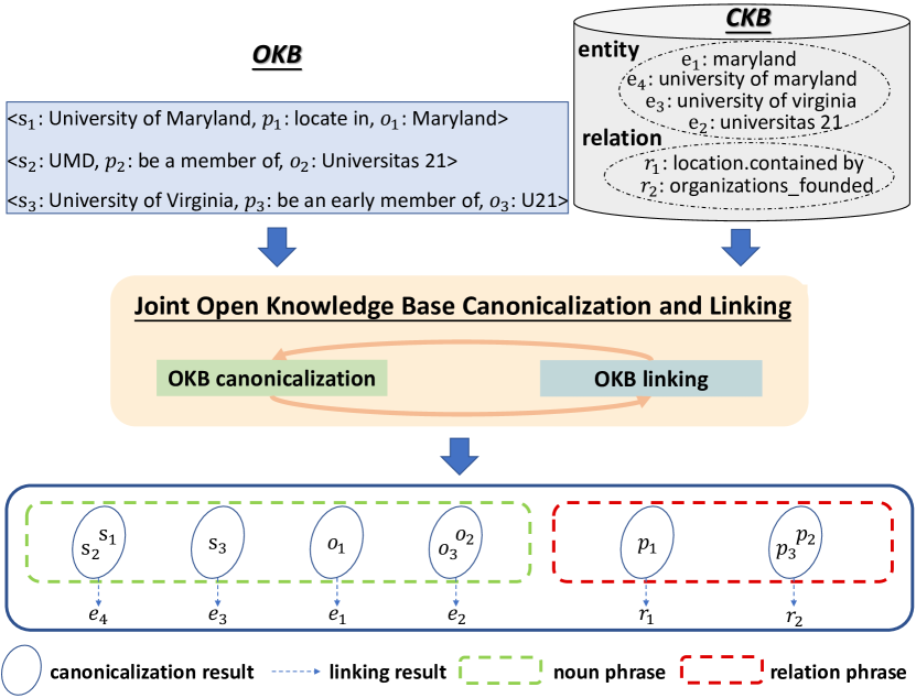
(a) An illustration for the task of joint OKB canonicalization and linking.

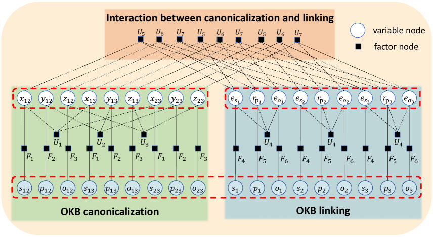
(b) A summarization of the proposed framework JOCL.

Figure 1. Task illustration and framework summarization.

OKB linking is the task to jointly link noun phrases and relation phrases in OIE triples, with their corresponding real world entities and relations in a CKB. Traditional joint entity and relation linking methods for text (Dubey et al., 2018; Sakor et al., 2019; Lin et al., 2020) perform poorly on OIE triples with limited context, which has been confirmed by our experiments.

From the two task definitions above, it can be seen that OKB canonicalization and OKB linking are closely related tasks. However, these two tasks have been studied in isolation so far. A heuristic way to integrate them is utilizing pipeline architecture, e.g., firstly canonicalizing OIE triples by an OKB canonicalization method, and then leveraging its output groups of noun phrases and relation phrases as the input for OKB linking. Unfortunately, as is common with pipeline architecture, errors from OKB canonicalization would propagate to OKB linking in this case. Any noun phrase or relation phrase that was wrongly grouped via OKB canonicalization clearly cannot be linked correctly by the downstream OKB linking model. In fact, these two tasks are tightly coupled and one task can benefit significantly from the kind of information provided by the other. The idea of our joint OKB canonicalization and linking is based on two assumptions as follows:

Assumption 1: Two noun phrases (relation phrases) in OIE triples are more likely to be clustered to the same group if they are linked to the same entity (relation) in a CKB via OKB linking.

Assumption 2: Two noun phrases (relation phrases) in OIE triples are more likely to be linked to the same entity (relation) in a CKB if they are clustered to the same group via OKB canonicalization.

It is observed that better OKB canonicalization result leads to better OKB linking result and vice versa. Meanwhile, errors made by one task may be corrected by the other. Therefore, in this paper, we propose to jointly solve OKB canonicalization and OKB linking, which faces the following challenges: (1) How to make these two tasks reinforce each other; (2) How to make use of all useful signals from both tasks; (3) How to make the framework flexible and able to extend to fit new signals of both tasks.

To address all the above issues, we propose a novel framework JOCL, which Jointly solves OKB Canonicalization and Linking based on factor graph model. Given a set of OIE triples in an OKB as well as a CKB, our framework firstly constructs a factor graph for each task respectively. With respect to the task of OKB canonicalization, JOCL generates a variable node for each pair of noun (relation) phrases to represent whether they have the same semantic meaning, and adds OKB canonicalization signals and transitive relation signals as factor nodes. With respect to the task of OKB linking, JOCL generates a variable node for each noun (relation) phrase to represent its corresponding entity (relation) in a CKB, and adds OKB linking signals and fact inclusion signals as factor nodes. Subsequently, in order to make these two tasks reinforce each other, consistency signals are added as factor nodes to perform the interaction between two tasks based on the two assumptions above. A reasonable working procedure (i.e., interact between two tasks after resolving them alone) is elaborately designed for the Loopy belief propagation (LBP) algorithm (Murphy et al., 1999; Kschischang et al., 2001; Ran et al., 2018) to pass messages among different types of nodes on the factor graph and learn parameters of our framework. With the final messages, JOCL could compute the marginal probability for each node according to the learned weights, and infer the corresponding entity (relation) for each noun (relation) phrase and generate canonicalization groups of noun (relation) phrases jointly. It is noted that due to intrinsic characteristics of factor graph model, our framework JOCL is flexible to fit any new signals via adding suitable factor nodes.

Our contributions can be summarized as follows:

• We are the first to explore the task of joint OKB canonicalization and linking, a new and increasingly important problem due to its broad applications.

• We propose a novel framework JOCL to perform OKB canonicalization and linking jointly, and make them reinforce each other. JOCL is flexible enough to combine different signals from two tasks together, and able to extend to fit any new signals of both tasks based on factor graph model.

• A thorough experimental study over two real-world data sets shows that JOCL outperforms all the baseline methods for both tasks in terms of average F1 and accuracy.

2. PRELIMINARIES AND NOTATIONS

In a CKB, an entity is denoted by $e$, a relation is denote by $r$, the set of entities is denoted by $E$, and the set of relations is denoted by $R$. A fact in a CKB can be denoted by $<$$e_{i}$, $r_{k}$, $e_{j}$$>$, where $e_{i}$, $e_{j}$ $\in$ $E$ and $r_{k}$ $\in$ $R$. In an OKB, an OIE triple is denoted by $t_{i}$=$<$$s_{i},p_{i},o_{i}$$>$, where $s_{i}$ and $o_{i}$ are noun phrases (NPs) and $p_{i}$ is a relation phrase (RP). A set of OIE triples is denoted by $T=\{t_{1},t_{2},...\}$.

Definition 0 (Joint OKB Canonicalization and Linking).

Given a set of OIE triples in an OKB and a CKB, the target of this joint task is to cluster NPs or RPs with the same semantic meaning into a group (i.e., OKB canonicalization) and meanwhile linking each group of NPs or RPs with their corresponding real world entity or relation in a CKB (i.e., OKB linking) jointly.

For illustration, we show a running example of this task in Figure 1(a). The input is three OIE triples and a CKB. With respect to the canonicalization result (marked with blue ellipses), we should cluster NPs into four groups and cluster RPs into two groups. With respect to the linking result (marked with blue arrows), we should link each group of NPs or RPs with their corresponding entity or relation in the CKB.

A factor graph consists of variable nodes, factor nodes, and edges. A variable node represents a random variable and a factor node represents a factor function among variable nodes. In our factor graph, we utilize exponential-linear functions to instantiate factor functions. A factor node and each of its related variable node are connected by an undirected edge. The two types of nodes in a factor graph form a bipartite and undirected graph.

3. The framework: JOCL

The overall framework JOCL is shown in Figure 1(b). We begin with the description of the factor graph for each task and then introduce the interaction between two tasks. Finally, we introduce the learning and inference algorithm of our framework.

3.1. OKB Canonicalization

OKB canonicalization consists of two subtasks, namely NP canonicalization and RP canonicalization. In this subsection we introduce the factor graph for the task of OKB canonicalization given a set of OIE triples in an OKB. We firstly introduce how to generate variable nodes and factor nodes for this task. Next, we introduce some useful signals of NP (RP) canonicalization and transitive relation, which are embedded in factor nodes.

3.1.1. Variable nodes

For any two OIE triples $t_{i}$ and $t_{j}$, three observed variable $s_{ij}$ ($p_{ij}$, $o_{ij}$) called subject (predicate, object) pair variables are used to represent the NP pair $(s_{i},s_{j})$, the RP pair $(p_{i},p_{j})$, and the NP pair $(o_{i},o_{j})$, respectively. Each observed variable has only one state as it is observed. We generate a variable node for each observed variable in the factor graph. Additionally, we define three canonicalization variables $x_{ij}$ ($y_{ij}$, $z_{ij}$) called subject (predicate, object) canonicalization variables, corresponding to the variables $s_{ij}$, $p_{ij}$, and $o_{ij}$ respectively. The canonicalization variable represents whether two NPs or RPs have the same semantic meaning. Therefore, each canonicalization variable has two states (i.e., 0 and 1). For example, $x_{ij}=1$ means NP $s_{i}$ and NP $s_{j}$ refer to the same entity. We generate a variable node for each canonicalization variable in the factor graph.

3.1.2. Factor nodes

We add six kinds of factor nodes: subject (predicate, object) canonicalization factor node $F_{1}$ ($F_{2}$, $F_{3}$), and subject (predicate, object) transitive relation factor node $U_{1}$ ($U_{2}$, $U_{3}$).

We utilize some NP canonicalization signals to define $F_{1}$ ($F_{3}$) as a factor function over a subject (object) pair variable and its corresponding subject (object) canonicalization variable, and generate a subject (object) canonicalization factor node for this function in the factor graph. We utilize some RP canonicalization signals to define $F_{2}$ as a factor function over a predicate pair variable and its corresponding relation canonicalization variable, and generate a predicate canonicalization factor node for this function in the factor graph. We utilize transitive relation signals to define a factor function $U_{1}$ ($U_{2}$, $U_{3}$) over three subject (relation, object) canonicalization variables that satisfy transitive relations, and generate a transitive relation factor node for this function in the factor graph.

3.1.3. NP canonicalization signals

• IDF token overlap: Inverse document frequency (IDF) token overlap is based on the assumption that two NPs sharing infrequent words are more likely to refer to the same object in the world. For example, it is likely that “Warren Buffett” and “Buffett” refer to the same entity which share an infrequent word “Buffett”. In (Galárraga et al., 2014) this signal has been verified to be a very effective signal for canonicalization and we use it to calculate the similarity between two NPs denoted by $Sim_{idf}(s_{i},s_{j})$ as follows.

  $$Sim_{idf}(s_{i},s_{j})=\frac{\sum\nolimits_{x\in w(s_{i})\cap w(s_{j})}log(1+f(x))^{-1}}{\sum\nolimits_{x\in w(s_{i})\cup w(s_{j})}log(1+f(x))^{-1}}$$

  where $w(\cdot)$ is the set of words of a string, and $f(x)$ is the frequency of the word $x$ in the collection of all words that appear in the NPs of the OIE triples. We define the feature function $f_{idf}$ based on $Sim_{idf}$ as follows.

  $$f_{idf}(s_{ij},x_{ij})=\begin{cases}Sim_{idf}(s_{i},s_{j})\text{\ \ \ \ \ \ if $x_{ij}=1$}\\ 1-Sim_{idf}(s_{i},s_{j})\text{\ \ \ if $x_{ij}=0$}\\ \end{cases}$$

• Word embedding: Word embeddings are the de-facto standard in language modeling and very popular in NLP. A word embedding maps words from a vocabulary to vectors of real numbers. Word embeddings are often learned from co-occurrences and neighborhoods of words in large corpora (Mikolov et al., 2013; Pennington et al., 2014). The rationale is that the meaning of a word is captured by the contexts where it often appears, which is called “distributional semantics”. For a NP which contains several words, we average the vectors of all the single words in the phrase as its embedding for simplicity. We use the cosine similarity to calculate the similarity between the embeddings of two NPs. The similarity between two NPs based on this signal can be denoted by $Sim_{emb}(s_{i},s_{j})$ and we define the feature function $f_{emb}$ based on it.

  $$f_{emb}(s_{ij},x_{ij})=\begin{cases}Sim_{emb}(s_{i},s_{j})\text{\ \ \ \ if $x_{ij}=1$}\\ 1-Sim_{emb}(s_{i},s_{j})\text{\ \ \ if $x_{ij}=0$}\\ \end{cases}$$

  For instance, the score of $Sim_{emb}$(“Barack Obama”, “President Obama”) is $0.873$ using fastText (Grave et al., 2018) embeddings trained on Common Crawl via MindSpore Framework, which indicates these two NPs are likely to refer to the same entity.

• PPDB: PPDB 2.0 (Pavlick et al., 2015) is a large collection of paraphrases in English. All the equivalent phrases are clustered into a group and each group is randomly assigned a representative. If two NPs have the same cluster representative according to the index, they are considered to be equivalent and we set value of similarity to $1$ otherwise $0$. The similarity between two NPs based on this signal can be denoted by $Sim_{PPDB}(s_{i},s_{j})$ and we define the feature function $f_{PPDB}$ based on it.

  $$f_{PPDB}(s_{ij},x_{ij})=\begin{cases}Sim_{PPDB}(s_{i},s_{j})\text{\ \ \ \ if $x_{ij}=1$}\\ 1-Sim_{PPDB}(s_{i},s_{j})\text{\ \ \ if $x_{ij}=0$}\\ \end{cases}$$

Lastly, we define $F_{1}$ based on all NP canonicalization signals.

$$F_{1}(s_{ij},x_{ij})=\frac{1}{Z_{1}}exp\{\boldsymbol{\alpha}_{1}^{T}\boldsymbol{f}_{1}(s_{ij},x_{ij})\},\ Z_{1}=\sum\limits_{x_{ij}}exp\{\boldsymbol{\alpha}_{1}^{T}\boldsymbol{f}_{1}(s_{ij},x_{ij})\}$$

where $\boldsymbol{f}_{1}$$=<$$f_{idf},f_{emb},f_{PPDB}$$>$ is a vector of feature functions; $\boldsymbol{\alpha}_{1}$ denotes the corresponding weights of the feature functions. Similarly, we can define $F_{3}$ based on the NP canonicalization signals above as well.

3.1.4. RP canonicalization signals

IDF token overlap, word embedding, and PPDB introduced above can be used as the RP canonicalization signals directly as well. Apart from these, inspired by (Vashishth et al., 2018) we use the following two additional signals.

• AMIE: AMIE algorithm (Galárraga et al., 2013) can judge whether two RPs represent the same semantic meaning by learning Horn rules. We take morphological normalized OIE triples as the input of AMIE, and the output of AMIE is a set of implication rules between two RPs $p_{i}$ and $p_{j}$ (e.g., $p_{i}\Rightarrow p_{j}$) based on statistical rule mining. If both $p_{i}\Rightarrow p_{j}$ and $p_{j}\Rightarrow p_{i}$ satisfy support and confidence thresholds, we consider two RPs (i.e., $p_{i}$ and $p_{j}$) have the same semantic meaning and set value of similarity to $1$ otherwise $0$. The similarity between two RPs using AMIE is denoted by $Sim_{AMIE}(p_{i},p_{j})$ and the feature function $f_{AMIE}$ can be defined based on it as follows.

  $$f_{AMIE}(p_{ij},y_{ij})=\begin{cases}Sim_{AMIE}(p_{i},p_{j})\text{\ \ \ \ if $y_{ij}=1$}\\ 1-Sim_{AMIE}(p_{i},p_{j})\text{\ \ \ if $y_{ij}=0$}\\ \end{cases}$$

  For instance, the score of $Sim_{AMIE}$(“is the capital of”, “is the capital city of”) is $1$ on the OIE triple data set ReVerb45K in our experiments, which indicates these two RPs have the same semantic meaning.

• KBP: Stanford Knowledge Base Population (KBP) (Surdeanu et al., 2012) system can link a RP to a relation in a CKB. If the relations of two RPs fall in the same category, these two RPs are considered as equivalent and we set value of similarity to $1$ otherwise $0$. The similarity between two RPs using KBP can be denoted by $Sim_{KBP}(p_{i},p_{j})$ and the feature function $f_{KBP}$ can be defined based on it as follows.

  $$f_{KBP}(p_{ij},y_{ij})=\begin{cases}Sim_{KBP}(p_{i},p_{j})\text{\ \ \ \ if $y_{ij}=1$}\\ 1-Sim_{KBP}(p_{i},p_{j})\text{\ \ \ if $y_{ij}=0$}\\ \end{cases}$$

  For example, the score of $Sim_{KBP}$(“was working at”, “worked for”) is $1$, which indicates these two RPs have the same semantic meaning.

Lastly, we define $F_{2}$ based on all RP canonicalization signals.

$$F_{2}(p_{ij},y_{ij})=\frac{1}{Z_{2}}exp\{\boldsymbol{\alpha}_{2}^{T}\boldsymbol{f}_{2}(p_{ij},y_{ij})\},\ Z_{2}=\sum\limits_{y_{ij}}exp\{\boldsymbol{\alpha}_{2}^{T}\boldsymbol{f}_{2}(p_{ij},y_{ij})\}$$

where $\boldsymbol{f}_{2}$$=$$<$$f_{idf}$, $f_{emb}$, $f_{PPDB}$, $f_{AMIE}$, $f_{KBP}$$>$ is a vector of feature functions; $\boldsymbol{\alpha}_{2}$ denotes the corresponding weights of the feature functions.

3.1.5. Transitive relation signals

We have the fact that the pairs satisfy transitive relations. As an example, if NP $s_{1}$ and NP $s_{2}$ have the same semantic meaning (i.e., canonicalization variable $x_{12}$$=$$1$), and $s_{2}$ and $s_{3}$ have the same semantic meaning (i.e., $x_{23}$$=$$1$), then we can deduce that $s_{1}$ and $s_{3}$ have the same semantic meaning (i.e., $x_{13}$$=$$1$). If values of this kind of three canonicalization variables satisfy transitive relations, they should be rewarded. If their values violate transitive relations, they should be penalized. Specifically, we define $u_{1}$ as a transitive relation feature function over three subject canonicalization variables $x_{ij}$, $x_{jk}$, and $x_{ik}$ that satisfy transitive relations. If values of all the three variables are 1 which case satisfies transitive relations, we will give a high score for $u_{1}$ heuristically. If only one of the three variables has a value of 0 and the other two are 1 which case violates transitive relations, we will give a low score heuristically. Otherwise, we will give a middle score. Scores range from $0$ to $1$. The high (middle, low) score is set to $0.9$ ($0.5$, $0.1$) in our experiments. We define the factor function $U_{1}$ as follows.

$$U_{1}(x_{ij},x_{jk},x_{ik})=\frac{1}{N_{1}}exp\{\boldsymbol{\beta}_{1}u_{1}(x_{ij},x_{jk},x_{ik})\}$$

where $N_{{}_{1}}$=$\sum\limits_{x_{ij},x_{jk},x_{ik}}exp\{\boldsymbol{\beta}_{1}u_{1}(x_{ij},x_{jk},x_{ik})\}$; $\boldsymbol{\beta}_{1}$ denotes the corresponding weight. We can define $U_{2}$ ($U_{3}$) based on the predicate (object) canonicalization variables in a similar way.

3.2. OKB Linking

OKB linking consists of two subtasks, namely OKB entity linking and OKB relation linking. In this subsection we introduce the factor graph for the task of OKB linking given a set of OIE triples in an OKB and a CKB. We firstly introduce how to generate variable nodes and factor nodes for this task. Next, we introduce some useful signals of OKB entity (relation) linking and fact inclusion, which are embedded in factor nodes.

3.2.1. Variable nodes

For an OIE triple $t_{i}$ in an OKB, we regard its NP $s_{i}$, RP $p_{i}$, and NP $o_{i}$ as three observed variables, namely subject variable, predicate variable, and object variable, respectively. Each observed variable only has one state as it is observed. We generate a variable node for each observed variable in the factor graph. Additionally, we define three linking variables $e_{s_{i}}$ ($r_{p_{i}}$, $e_{o_{i}}$) called subject (predicate, object) linking variables, corresponding to the observed variables $s_{i}$, $p_{i}$, and $o_{i}$, respectively. $e_{s_{i}}$ ($e_{o_{i}}$) represents the semantically corresponding entity existing in the CKB for NP $s_{i}$ ($o_{i}$) which has $|e_{s_{i}}|$ ($|e_{o_{i}}|$) possible states each of which is a candidate entity in the CKB that NP $s_{i}$ ($o_{i}$) may refer to. $r_{p_{i}}$ represents the semantically corresponding relation existing in the CKB for RP $p_{i}$. It has $|r_{p_{i}}|$ possible states each of which is a candidate relation in the CKB that $p_{i}$ may refer to. We generate a variable node for each linking variable in the factor graph.

3.2.2. Factor nodes

We add four kinds of factor nodes: subject (predicate, object) linking factor node $F_{4}$ ($F_{5}$, $F_{6}$), and fact inclusion factor node $U_{4}$.

We utilize some OKB entity linking signals to define $F_{4}$ ($F_{6}$) as a factor function over a subject (object) variable and its corresponding subject (object) linking variable, and generate a subject (object) linking factor node for this function in the factor graph. We utilize some OKB relation linking signals to define $F_{5}$ as a factor function over a predicate variable and its corresponding predicate linking variable, and generate a predicate linking factor node for this function in the factor graph. We utilize fact inclusion signals to define a factor function $U_{4}$ over a subject linking variable, a predicate linking variable, and an object linking variable that correspond to the same OIE triple, and generate a fact inclusion factor node for this function in the factor graph.

3.2.3. OKB entity linking signals

• Entity popularity: The entity popularity is found to be very helpful in previous entity linking methods (Shen et al., 2014, 2018; Ran et al., 2018; Guo et al., 2013; Hua et al., 2015; Hoffart et al., 2011), which tells us the prior probability of the appearance of a candidate entity given an entity mention. Thus, we utilize entity popularity as a signal of OKB entity linking. We use anchor links in Wikipedia to calculate the popularity of a candidate entity given a NP and define the feature function $f_{pop}$ as follows.

  $$f_{pop}(s_{i},e_{s_{i}})=\frac{count(s_{i},e_{s_{i}})}{count(s_{i})}$$

  where count($s_{i}$) denotes the number of the subject $s_{i}$ occurring as the surface form of an anchor link in Wikipedia; count($s_{i},e_{s_{i}}$) represents the number of anchor links with the surface form $s_{i}$ pointing to the candidate entity $e_{s_{i}}$.

We also use word embedding and PPDB introduced in Section 3.1.3 as other two OKB entity linking signals by computing string similarity between surface forms of the subject $s_{i}$ and its candidate entity $e_{s_{i}}$. Specifically, their corresponding feature functions are defined as: $f^{\prime}_{emb}(s_{i},e_{s_{i}})=Sim_{emb}(s_{i},e_{s_{i}})$ and $f^{\prime}_{PPDB}(s_{i},e_{s_{i}})=Sim_{PPDB}(s_{i},e_{s_{i}})$. Lastly, we define $F_{4}$ based on all OKB entity linking signals.

$$F_{4}(s_{i},e_{s_{i}})=\frac{1}{Z_{4}}exp\{\boldsymbol{\alpha}_{4}^{T}\boldsymbol{f}_{4}(s_{i},e_{s_{i}})\},\ Z_{4}=\sum\limits_{e_{s_{i}}}exp\{\boldsymbol{\alpha}_{4}^{T}\boldsymbol{f}_{4}(s_{i},e_{s_{i}})\}$$

where $\boldsymbol{f}_{4}=$$<$$f_{pop}$,$f^{\prime}_{emb}$,$f^{\prime}_{PPDB}$$>$ is a vector of feature functions; $\boldsymbol{\alpha}_{4}$ denotes the corresponding weights of the feature functions. Similarly, we can define $F_{6}$ based on the OKB entity linking signals above as well.

3.2.4. OKB relation linking signals

Word embedding and PPDB introduce above can be used as the OKB relation linking signals directly as well. Besides these, we use the following two signals.

• Ngram (Nakashole et al., 2013): Ngram can convert a string into a set of ngrams (i.e., a sequence of n characters). The similarity between strings based on ngram could be Jaccard similarity between their sets of ngrams.

• Levenshtein distance (LD): LD can calculate the number of deletions, insertions, or substitutions required to transform a string into another string, which could be regarded as the distance between strings. We normalize LD to a range from $0$ to $1$.

We define the feature functions $f_{ngram}(p_{i},r_{p_{i}})$ and $f_{LD}(p_{i},r_{p_{i}})$ by computing string similarity between surface forms of the predicate $p_{i}$ and its candidate relation $r_{p_{i}}$ via ngram and LD, respectively. We adopt a python library to compute those different string similarities in our experiments. Lastly, we define $F_{5}$ based on all OKB relation linking signals.

$$F_{5}(p_{i},r_{p_{i}})=\frac{1}{Z_{5}}exp\{\boldsymbol{\alpha}_{5}^{T}\boldsymbol{f}_{5}(p_{i},r_{p_{i}})\},\ Z_{5}=\sum\limits_{r_{p_{i}}}exp\{\boldsymbol{\alpha}_{5}^{T}\boldsymbol{f}_{5}(p_{i},r_{p_{i}})\}$$

where $\boldsymbol{f}_{5}$=$<$$f_{ngram}$, $f_{LD}$, $f^{\prime}_{emb}$,$f^{\prime}_{PPDB}$$>$ is a vector of feature functions; $\boldsymbol{\alpha}_{5}$ defines the corresponding weights of the feature functions.

3.2.5. Fact inclusion signals

For an OIE triple, its corresponding entities and relation are likely to compose a triple already included in a CKB. Therefore, if values of linking variables with respect to an OIE triple $t_{i}$=$<$$s_{i},p_{i},o_{i}$$>$ compose a triple already included in a CKB, they should be rewarded. Specifically, we define $u_{4}$ as a fact inclusion feature function over three linking variables $e_{s_{i}}$, $r_{p_{i}}$, and $e_{o_{i}}$ with respect to an OIE triple $t_{i}$=$<$$s_{i},p_{i},o_{i}$$>$. If the triple $(e_{s_{i}},r_{p_{i}},e_{o_{i}})$ is a fact already included in a CKB, we will give a high score for $u_{4}$ heuristically otherwise a relatively low score. Scores range from $0$ to $1$. The high (low) score is set to $0.9$ ($0.1$) in our experiments. We define the factor function $U_{4}$ as follows.

$$U_{4}(e_{s_{i}},r_{p_{i}},e_{o_{i}})=\frac{1}{N_{4}}exp\{\boldsymbol{\beta}_{4}u_{4}(e_{s_{i}},r_{p_{i}},e_{o_{i}})\}$$

where $N_{4}$=$\sum\limits_{e_{s_{i}},r_{p_{i}},e_{o_{i}}}$$exp\{\boldsymbol{\beta}_{4}u_{4}(e_{s_{i}},r_{p_{i}},e_{o_{i}})\}$; $\boldsymbol{\beta}_{4}$ denotes the corresponding weight.

3.3. Interaction Between Two Tasks

To make two tasks reinforce each other, we utilize consistency signals to define a factor function $U_{5}$ ($U_{6}$, $U_{7}$) over a subject (predicate, object) canonicalization variable and its corresponding two subject (predicate, object) linking variables, and generate a consistency factor node for this function in the factor graph.

Based on the two assumptions introduced in Section 1, we come to the conclusion that OKB canonicalization result and OKB linking result should be consistent. For example, if NP $s_{1}$ and NP $s_{2}$ are linked to the same entity in a CKB (i.e., $e_{s_{1}}$$=$$e_{s_{2}}$), they should have the same semantic meaning (i.e., $x_{12}$$=$$1$) and vice versa. If values of these corresponding variables satisfy consistency relations, they should be rewarded. Otherwise, they should be penalized. Specifically, we define $u_{5}$ as a consistency feature function over three variables $e_{s_{i}}$, $e_{s_{j}}$, and $x_{ij}$. If the value of $e_{s_{i}}$ equals the value of $e_{s_{j}}$ and the value of $x_{ij}$ is $1$, or the value of $e_{s_{i}}$ does not equal the value of $e_{s_{j}}$ and the value of $x_{ij}$ is $0$ which two cases satisfy consistency relations, we will give a high score for $u_{5}$ heuristically. Otherwise, we set a relatively low score heuristically. Scores range from $0$ to $1$. The high (low) score is set to $0.7$ ($0.3$) in our experiments. Then we define the factor function $U_{5}$ as follows.

$$U_{5}(e_{s_{i}},e_{s_{j}},x_{ij})=\frac{1}{N_{5}}exp\{\boldsymbol{\beta}_{5}u_{5}(e_{s_{i}},e_{s_{j}},x_{ij})\}$$

where $N_{5}$=$\sum\limits_{e_{s_{i}},e_{s_{j}},x_{ij}}$$exp\{\boldsymbol{\beta}_{5}u_{5}(e_{s_{i}},e_{s_{j}},x_{ij})\}$; $\boldsymbol{\beta}_{5}$ denotes the corresponding weight. We can define $U_{6}$ ($U_{7}$) based on a predicate (object) canonicalization variable and its corresponding two predicate (object) linking variables in a similar way.

3.4. Learning

For our model, the factor function of any factor node can be represented in a unified form as $H_{j}$:

(1) $$H_{j}(C_{j})=\frac{1}{Z_{j}}exp\{\boldsymbol{\omega}^{T}\boldsymbol{h}_{j}(C_{j})\}$$

where $j$ denotes a clique which is a fully connected subset of the variables in the graph, $C_{j}$ is the set of variable nodes in the clique $j$, $\boldsymbol{\omega}=(\omega_{1},\omega_{2},...)$ is a weighting vector and $\boldsymbol{h}_{j}$ is a vector of feature functions. Learning a factor graph model is to estimate an optimum parameter configuration $\boldsymbol{\omega}^{*}$.

According to the factorization principle in the factor graph (Kschischang et al., 2001), we could use the product of these factor functions to represent the joint probability over variables as follows.

(2) $$P(Y)=\frac{1}{Z}\prod_{j}H_{j}(C_{j}),\ Z=\sum\limits_{C_{j}}\prod_{j}H_{j}(C_{j})$$

where $Z$ is a normalization factor, which is the summation of all possible values for $C_{j}$. $Y$ is defined as a collection of variables in our framework as follows.

(3) $$Y=\{e_{s_{i}},r_{p_{i}},e_{o_{i}},x_{ij},y_{ij},z_{ij},e_{s_{j}},r_{p_{j}},e_{o_{j}}\}$$

where $t_{i}=<s_{i},p_{i},o_{i}>$, $t_{j}=<s_{j},p_{j},o_{j}>$, and $t_{i},t_{j}\in T$. We use $P(Y)$ as the object function of our task and rewrite this function according to Formula 1 as follows.

(4) $$P(Y)=\frac{1}{Z^{\prime}}exp\{\boldsymbol{\omega}^{T}\sum\limits_{j}h_{j}(C_{j})\}=\frac{1}{Z^{\prime}}exp\{\boldsymbol{\omega}^{T}Q\}$$

where $Z^{\prime}=\sum_{j}exp\{\boldsymbol{\omega}^{T}Q\}$ and $Q=\sum_{j}h_{j}(C_{j})$. We can obtain the following log-likelihood objective function:

(5) $$O(\boldsymbol{\omega}) =logP(Y^{L})=log\sum\limits_{Y|Y^{L}}\frac{1}{Z^{\prime}}exp\{\boldsymbol{\omega}^{T}Q\}$$

$$=log\sum\limits_{Y|Y^{L}}exp\{\boldsymbol{\omega}^{T}Q\}-log\sum\limits_{Y}exp\{\boldsymbol{\omega}^{T}Q\}$$

where $Y^{L}$ denotes the known labels and $Y|Y^{L}$ is a labeling configuration of $Y$ inferred from $Y^{L}$. We use the gradient descent algorithm to maximize the objective function. The gradient for parameters $\boldsymbol{\omega}$ can be calculated as follows:

(6) $$\frac{\partial{O(\boldsymbol{\omega})}}{\partial\boldsymbol{\omega}} =\frac{\partial{(log\sum_{Y|Y^{L}}exp\{\boldsymbol{\omega}^{T}Q\}-log\sum_{Y}exp\{\boldsymbol{\omega}^{T}Q\})}}{\partial\boldsymbol{\omega}}$$

$$=\frac{\sum_{Y|Y^{L}}exp\{\boldsymbol{\omega}^{T}Q\}\cdot{Q}}{\sum_{Y|Y^{L}}exp\{\boldsymbol{\omega}^{T}Q\}}-\frac{\sum_{Y}exp\{\boldsymbol{\omega}^{T}Q\}\cdot{Q}}{\sum_{Y}exp\{\boldsymbol{\omega}^{T}Q\}}$$

$$=\mathbb{E}_{p_{\boldsymbol{\omega}}(Y|Y^{L})}Q-\mathbb{E}_{p_{\boldsymbol{\omega}}(Y)}Q$$

where $\mathbb{E}_{p_{\boldsymbol{\omega}}(Y|Y^{L})}Q$ and $\mathbb{E}_{p_{\boldsymbol{\omega}}(Y)}Q$ are two expectations of $Q$ based on the probabilistic distribution $p_{\boldsymbol{\omega}}(Y|Y^{L})$ and $p_{\boldsymbol{\omega}}(Y)$ respectively. To obtain the gradient, we need to calculate two marginal probabilities $p(y_{i})$ and $p(y_{i},y_{j},y_{k})$, where $y_{i},y_{j},y_{k}\in{Y}$. However, as the graph structure of the factor graph can be arbitrary and may contain cycles, we cannot calculate the exact marginal probabilities. We use a two-step LBP algorithm to approximate the marginal probabilities. Interested readers please refer to (Tang et al., 2011, 2016; Ran et al., 2018) for details of the algorithm.

Specifically, we design a reasonable working procedure for the LBP algorithm based on the structure characteristics of our factor graph. We conduct the process of the message passing from factor nodes to variable nodes as follows.

• Update all the messages from canonicalization factor nodes to canonicalization variable nodes (i.e., $F_{1}$$\rightarrow$${x_{ij}}$, $F_{2}$$\rightarrow$${y_{ij}}$, $F_{3}$$\rightarrow$${z_{ij}}$).

• Update all the messages from transitive relation factor nodes to canonicalization variable nodes (i.e., $U_{1}$$\rightarrow$$x_{ij},x_{jk},x_{ik}\ \$ $U_{2}$$\rightarrow y_{ij}$,$y_{jk}$,$y_{ik}\ \$ $U_{3}$$\rightarrow$$z_{ij}$,$z_{jk}$,$z_{ik}$).

• Update all the messages from linking factor nodes to linking variable nodes (i.e., $F_{4}$$\rightarrow$$e_{s_{i}}$, $F_{5}$$\rightarrow$$r_{p_{i}}$, $F_{6}$$\rightarrow$$e_{o_{i}}$).

• Update all the messages from fact inclusion factor nodes to linking variable nodes (i.e., $U_{4}\rightarrow$$e_{s_{i}},r_{p_{i}},e_{o_{i}}$).

• Update all the messages from consistency factor nodes to canonicalization variable nodes and linking variable nodes (i.e., $U_{5}\rightarrow{e_{s_{i}},e_{s_{j}},x_{ij}}\ \ U_{6}\rightarrow{r_{p_{i}},r_{p_{j}},y_{ij}}\ \ U_{7}\rightarrow{e_{o_{i}},e_{o_{j}},z_{ij}}$).

For the process of the message passing from variable nodes to factor nodes, we firstly update all the messages from canonicalization variable nodes to each of their related factor nodes and then update all the messages from linking variable nodes to each of their related factor nodes.

With the marginal probabilities, the gradient can be obtained by summing over all variables. In practice we found that convergence was achieved within twenty iterations. The learning algorithm also can be extended to a distributed learning version with a graph segmentation algorithm such as (Jo et al., 2018).

3.5. Inference

After we learned the optimal parameters, we can infer the best label of each variable (i.e., the corresponding entity (relation) that each NP (RP) refers to, and whether two NPs or RPs represent the same semantic meaning) by computing the marginal probability for each node with the final messages. The best label could be the state with the highest marginal probability.

Although the consistency signals tend to make the results of OKB canonicalization and OKB linking as consistent as possible, there are still some conflicts between them after the process of inference. To eliminate conflicts and generate the final result, we design an intuitive method. If a pair of NPs are located in two different groups according to the linking result and the corresponding canonicalization variable of this pair has a value of 1, we select the label of the larger group as the final label for both NPs. Finally, we will obtain canonicalization groups of NPs (RPs) and the corresponding entity (relation) in a CKB for each group of NPs (RPs).

Table 1. Performance on the NP canonicalization task. All the results of the baselines are taken from SIST (Lin and Chen, 2019).

Method	ReVerb45K				NYTimes2018
	Macro F1	Micro F1	Pairwise F1	Average F1	Macro F1	Micro F1	Pairwise F1	Average F1
Morph Norm(2011) (Fader et al., 2011)	0.281	0.699	0.653	0.544	0.471	0.658	0.643	0.591
Wikidata Integrator	0.563	0.839	0.783	0.728	0.476	0.839	0.783	0.699
Text Similarity(2014) (Galárraga et al., 2014)	0.543	0.821	0.689	0.684	0.581	0.796	0.658	0.678
IDF Token Overlap(2014) (Galárraga et al., 2014)	0.598	0.571	0.505	0.558	0.551	0.612	0.527	0.563
Attriubte Overlap(2014) (Galárraga et al., 2014)	0.598	0.599	0.587	0.595	0.551	0.612	0.527	0.563
CESI(2018) (Vashishth et al., 2018)	0.618	0.845	0.819	0.761	0.586	0.842	0.778	0.735
SIST(2019) (Lin and Chen, 2019)	0.691	0.889	0.823	0.801	0.675	0.816	0.838	0.776
JOCL	0.684	0.892	0.877	0.818	0.561	0.921	0.934	0.805

Table 2. Performance on the RP canonicalization task. All the results of the baselines are taken from SIST (Lin and Chen, 2019).

Method	Macro F1	Micro F1	Pairwise F1	Average F1
AMIE(2013) (Galárraga et al., 2013)	0.703	0.820	0.760	0.761
PATTY(2012) (Nakashole et al., 2012)	0.782	0.872	0.802	0.819
SIST(2019) (Lin and Chen, 2019)	0.875	0.872	0.845	0.864
JOCL	0.848	0.923	0.851	0.874

4. EXPERIMENTAL STUDY

4.1. Experiment Settings

Two large scale publicly available OIE triple data sets are used in the experiments: ReVerb45K (Vashishth et al., 2018) and NYTimes2018 (Lin and Chen, 2019) which are common benchmark data sets for OKB canonicalization and OKB linking. The OIE triples of ReVerb45K are extracted by ReVerb (Fader et al., 2011) from the source text in Clueweb09 and all NPs are annotated with their corresponding Freebase entities. ReVerb45K contains $45$K triples all associated with Freebase entities each of which has at least two aliases occurring as NP. The OIE triples of NYTimes2018 are extracted by Standford OIE Tool (Angeli et al., 2015) over $1500$ articles from nytimes.com in $2018$. NYTimes2018 contains $34$K triples which are not annotated with any CKB. In both data sets, no training set is given. We leverage the triples associated with $20\%$ selected Freebase entities of ReVerb45K as the validation set, and the rest triples of ReVerb45K and all the triples of NYTimes2018 as two test sets. In this experiment, we use the validation set to train the parameters of our framework, and the test set to evaluate the performance.

For the task of OKB canonicalization, we adopt the same evaluation measures (i.e., macro, micro, and pairwise metrics) as previous works (Galárraga et al., 2014; Vashishth et al., 2018; Lin and Chen, 2019). Specifically, macro metric evaluates whether the NPs or RPs with the same semantic meaning have been clustered into a group, micro metric evaluates the purity of the resulting groups, and pairwise metric evaluates individual pairwise merging decisions. In each metric, F1 score is the harmonic mean of precision and recall. For the detailed computing methods of these metrics, we omit them due to limited space and you could refer to (Galárraga et al., 2014; Vashishth et al., 2018; Lin and Chen, 2019). To give an overall evaluation of each method for OKB canonicalization, we calculate average F1 as the average of macro F1, micro F1, and pairwise F1, which is common practice in OKB canonicalization. For the evaluation measure of OKB linking, we adopt accuracy which is a common measure for entity linking systems (Shen et al., 2015) and calculated as the number of correctly linked NPs (RPs) divided by the total number of all NPs (RPs). As it is unnecessary and impractical to generate canonicalization variables for all pairs of NPs and RPs in the factor graph, we generate canonicalization variables only for NP (RP) pairs with a relatively high similarity based on IDF token overlap introduced in Section 3.1.3, whose threshold is set to $0.5$. The learning rate of the gradient descent algorithm is set to $0.05$ in all experiments. The source code and data sets used in this paper are publicly available.

4.2. OKB Canonicalization Task

4.2.1. NP canonicalization

The baselines are listed as follows.

• Morph Norm (Fader et al., 2011) uses some simple normalization operations (e.g., removing tenses, pluralization).

• Wikidata Integrator is an opensource entity linking tool. NPs linked to the same entity by it are grouped together.

• Text Similarity (Galárraga et al., 2014) calculates the similarity between two NPs by JaroWinkler (Winkler, 1999) similarity and utilizes hierarchical agglomerative clustering (HAC) method.

• IDF Token Overlap (Galárraga et al., 2014) calculates the similarity between two NPs based on IDF token overlap and utilizes HAC method for clustering.

• Attribute Overlap (Galárraga et al., 2014) uses the Jaccard similarity of attributes between two NPs for canonicalization.

• CESI (Vashishth et al., 2018) performs OKB canonicalization using learned embeddings and side information.

• SIST (Lin and Chen, 2019) is the state-of-the-art method for OKB canonicalization by leveraging side information from the original source text.

Specially, for NYTimes2018 data set which is not annotated with any CKB, we randomly sample 100 non-singleton NP groups and manually label them as the ground truth for NP canonicalization like SIST. From the results shown in Table 1, we can see that JOCL outperforms all the baselines in terms of average F1 on both data sets. CESI improves the quality of the NP canonicalization by using various side information (e.g., Wordnet, PPDB, and KBP). SIST outperforms CESI by leveraging more side information from the original source text, which puts JOCL at a disadvantage. However, in spite of this disadvantage, JOCL still promotes by about $1.7$ ($2.9$) percentages compared with SIST in terms of average F1 over ReVerb45K (NYTimes2018), which demonstrates the effectiveness of JOCL in NP canonicalization.

4.2.2. RP canonicalization

We utilize AMIE introduced in Section 3.1.4, PATTY (Nakashole et al., 2012), and SIST as baselines of RP canonicalization over ReVerb45K. PATTY can put the triples with the same pairs of NPs, as well as RPs that belong to the same synset in PATTY in one group. We randomly sample 35 non-singleton RP groups and manually label them as the ground truth for RP canonicalization, which is the same as SIST. If two RPs have the same meaning after removing tense, pluralization, auxiliary verb, determiner, and modifier, they are considered to be the same. As shown in Table 2, compared with AMIE, our framework and other two baselines (i.e., PATTY and SIST) perform better, since the number of appearance for most RPs is less than the support threshold which leads AMIE only covers very few RPs. Compared with the state-of-the-art method SIST, JOCL promotes by about $1$ percentage in terms of average F1, which demonstrates the effectiveness of JOCL in RP canonicalization.

Table 3. Performance on OKB entity linking task.

Method	$\boldsymbol{\mathit{ReVerb45K}}$	$\boldsymbol{\mathit{NYTimes2018}}$
$\rm Falcon$	$0.541$	0.33
$\rm EARL$	0.473	0.25
Spotlight	0.716	0.26
$\rm Tagme$	$0.316$	0.3
$\rm KBPearl$	$0.522$	0.46
$\rm JOCL$	0.761	0.48

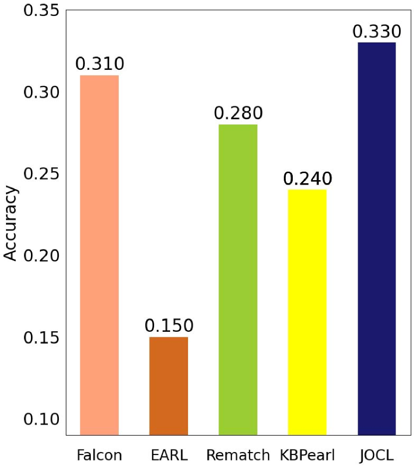
Figure 3: Performance on OKB relation linking task.

Table 4. Performance of JOCL working separately for each task.

Variant	$\boldsymbol{\mathit{Macro\ F1}}$	$\boldsymbol{\mathit{Micro\ F1}}$	$\boldsymbol{\mathit{Pairwise\ F1}}$	$\boldsymbol{\mathit{Average\ F1}}$	$\boldsymbol{\mathit{Accuracy}}$
$\rm JOCL_{cano}$	$0.571$	$0.846$	$0.787$	$0.735$	-
$\rm JOCL_{link}$	-	-	-	-	$0.744$
JOCL	0.684	0.892	0.877	0.818	0.761

4.3. OKB Linking Task

4.3.1. OKB entity linking

The baselines are listed as follows.

• Spotlight (Daiber et al., 2013; Mendes et al., 2011) is a popular baseline for entity linking based on DBpedia.

• TagMe (Ferragina and Scaiella, 2010) is a popular baseline in the TAC KBP data sets for entity linking (Ji et al., 2014; Raiman and Raiman, 2018).

• Falcon (Sakor et al., 2019) performs joint entity and relation linking using some fundamental principles of English morphology.

• EARL (Dubey et al., 2018) performs joint entity and relation linking by solving a Generalized Traveling Salesman Problem (GTSP).

• KBPearl (Lin et al., 2020) is a joint entity and relation linking system leveraging the context knowledge of the triples and side information inferred from the source text.

Specially, for NYTimes2018 data set that is unlabeled, we randomly sample $100$ OIE triples and manually label each NP with its gold mapping entity as the ground truth for OKB entity linking task. For each baseline, we show its best performing result under its best parameter setting via running its different settings in Table 3. From the results on both data sets in Table 3, it can be seen that our framework JOCL outperforms all the five baselines on both data sets, which demonstrates the effectiveness of our framework for the task of OKB entity linking.

4.3.2. OKB relation linking

Falcon, EARL, and KBPearl can be used as the baselines of OKB relation linking as well. Apart from these, we use Rematch (Mulang et al., 2017) which is one of the top-performing tools for the relation linking task as a baseline. We randomly sample $100$ OIE triples of ReVerb45K and manually label each RP as the ground truth for OKB relation linking task. For each baseline, we show its best performing result under its best parameter setting in Figure 3. It can be seen that JOCL outperforms all the four baselines. The performance of all the methods on this task is not well compared with the OKB entity linking task, since the relations expressed in the OIE triples have much more representations than entities which makes this task very challenging.

4.4. Effect Analysis of Interaction Between Two Tasks

To verify the effectiveness of interaction between two tasks, we remove consistency factor nodes introduced in Section 3.3 from JOCL and make these two tasks unable to interact with each other. We present the performance of two variants, namely, $\rm JOCL_{cano}$ (i.e., JOCL working on OKB canonicalization task alone) and $\rm JOCL_{link}$ (i.e., JOCL working on OKB linking task alone), as well as the whole framework JOCL on ReVerb45K in Table 4. From the experimental results, we can see that JOCL outperforms $\rm JOCL_{cano}$ ($\rm JOCL_{link}$) in terms of average F1 (accuracy) over OKB canonicalization (linking) task, which demonstrates that the whole framework JOCL could indeed perform the interaction between two tasks effectively and make them reinforce each other obviously. For the canonicalization task, $\rm JOCL_{cano}$ outperforms most baselines except CESI and SIST in terms of average F1 shown in Table 1, since these two outperforming baselines use extra context knowledge inferred from the source text. For the linking task, $\rm JOCL_{link}$ outperforms all the baselines in terms of accuracy shown in Table 3.

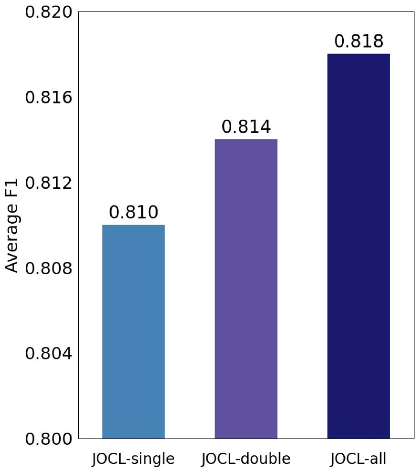
(a) NP canonicalization.

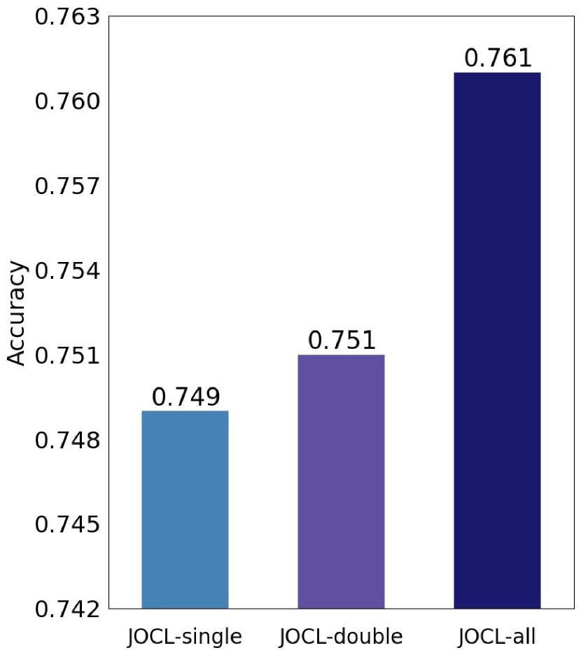
(b) OKB entity linking.

Figure 4: Performance of different variants of JOCL for feature effect analysis.

4.5. Effect Analysis of Different Combinations of Feature Functions

We define three different variants of our framework JOCL (i.e., JOCL-single, JOCL-double, JOCL-all) shown in Table 5 by leveraging different combinations of the feature functions for each factor function in the factor graph, and present their performance on the NP canonicalization task (i.e., Figure 4(a)) and on the OKB entity linking task (i.e., Figure 4(b)) over ReVerb45K, respectively. From the experimental results, we can see that JOCL-all leveraging all the feature functions of each factor function achieves the best performance for both tasks. The more useful signals, the better the performance, which is consistent with our intuition. Moreover, we can see that JOCL is flexible enough to combine different signals from two tasks and able to extend to fit any new signals.

Table 5. Different variants of JOCL for feature effect analysis.

Variant	$\boldsymbol{\mathit{F_{1}}}$, $\boldsymbol{\mathit{F_{3}}}$	$\boldsymbol{\mathit{F_{2}}}$	$\boldsymbol{\mathit{F_{4}}}$, $\boldsymbol{\mathit{F_{6}}}$	$\boldsymbol{\mathit{F_{5}}}$
JOCL-single	$f_{idf}$	$f_{idf}$	$f_{pop}$	$f_{ngram}$
JOCL-double	$f_{idf},f_{emb}$	$f_{idf},f_{emb}$	$f_{pop},f^{\prime}_{emb}$	$f_{ngram},f^{\prime}_{emb}$
JOCL-all	$\boldsymbol{f}_{1}$	$\boldsymbol{f}_{2}$	$\boldsymbol{f}_{4}$	$\boldsymbol{f}_{5}$

5. related work

Four aspects of research are related to our work: OKB canonicalization, OKB linking, factor graph model, and entity resolution, which are introduced in detail as follows.

The first work for OKB canonicalization (Galárraga et al., 2014) clusters NPs using some manually-defined signals to obtain equivalent NPs, and clusters RPs based on rules discovered by AMIE (Galárraga et al., 2013). FAC (Wu et al., 2018) proposes a more efficient graph-based clustering method by pruning and bounding techniques. CESI (Vashishth et al., 2018) learns the embeddings of NPs and RPs leveraging side information in a principled manner and clusters the learned embeddings together to obtain canonicalized NP (RP) groups. SIST (Lin and Chen, 2019) proposes to leverage side information from the original source text (i.e., candidate entities of NPs, types of candidate entities, and the domain knowledge of the source text) to further improve the OKB canonicalization result.

The most related work to OKB linking is the task of joint entity and relation linking. EARL (Dubey et al., 2018) designs two solutions: (1) formalizes the joint entity and relation linking tasks as an instance of the GTSP; (2) exploits the connection density between nodes in the graph. Falcon (Sakor et al., 2019) utilizes the fundamental principles of English morphology (e.g., compounding and headword identification) and an extended knowledge graph created by merging entities and relations from various knowledge sources to capture semantics underlying the text. KBPearl (Lin et al., 2020) performs joint entity and relation linking utilizing the context knowledge of the triples and side information extracted from the source documents. KBPearl relies on the source document, while our JOCL only focuses on the OIE triples without requiring the original source text.

The factor graph model has been successfully applied in many applications, such as knowledge base alignment (Wang et al., 2012), social relationship mining (Tang et al., 2011, 2016), social influence analysis (Tang et al., 2009), Web table annotation(Limaye et al., 2010; Zhang and Chakrabarti, 2013), co-investment of venture capital (Wang et al., 2015), relationship prediction in E-commerce platform (Cen et al., 2019), and tweet entity linking (Ran et al., 2018). In this paper, we apply the factor graph model to jointly solve OKB canonicalization and OKB linking successfully.

The task of entity resolution (Elmagarmid et al., 2006; Getoor and Machanavajjhala, 2012; Mudgal et al., 2018) is related but different from our task. In entity resolution, each record describing an entity that needs to be matched contains a set of attribute values of this entity, while in our task the NPs and RPs that need to be clustered and linked reside in OIE triples and do not have attribute values with them.

6. conclusion

OKB canonicalization and OKB linking are tightly coupled tasks, and one task can benefit significantly from the other. However, previous studies only focus on one of them and cannot solve them jointly. To achieve this goal, we propose a novel framework JOCL based on factor graph model to perform interaction between two tasks and make them reinforce each other. JOCL can combine signals from both tasks and extend to fit new signals. To demonstrate the effectiveness of JOCL, we conduct experiments over two large scale OIE triple data sets and the experimental results show that our framework outperforms all the baselines for both tasks in terms of average F1 and accuracy.

7. Acknowledgments

This work was supported in part by National Natural Science Foundation of China (No. U1936206, 61772289), Natural Science Foundation of Tianjin (No. 19JCQNJC00100), YESS by CAST (No. 2019QNRC001), and CAAI-Huawei MindSpore Open Fund. Jianyong Wang was supported in part by National Key Research and Development Program of China (No. 2020YFA0804503), National Natural Science Foundation of China (No. 61532010, 61521002), and Beijing Academy of Artificial Intelligence (BAAI).

References

- (1)
- Angeli et al. (2015) Gabor Angeli, Melvin Jose Johnson Premkumar, and Christopher D Manning. 2015. Leveraging linguistic structure for open domain information extraction. In ACL. 344–354.
- Banko et al. (2007) Michele Banko, Michael J. Cafarella, Stephen Soderland, Matthew Broadhead, and Oren Etzioni. 2007. Open information extraction from the web. In IJCAI. 2670–2676.
- Bollacker et al. (2008) Kurt Bollacker, Colin Evans, Praveen Paritosh, Tim Sturge, and Jamie Taylor. 2008. Freebase: a collaboratively created graph database for structuring human knowledge. In SIGMOD. 1247–1250.
- Cao et al. (2020) Ermei Cao, Difeng Wang, Jiacheng Huang, and Wei Hu. 2020. Open Knowledge Enrichment for Long-tail Entities. In WWW. 384–394.
- Cen et al. (2019) Yukuo Cen, Jing Zhang, Gaofei Wang, Yujie Qian, Chuizheng Meng, Zonghong Dai, Hongxia Yang, and Jie Tang. 2019. Trust Relationship Prediction in Alibaba E-Commerce Platform. IEEE Transactions on Knowledge and Data Engineering 32, 5 (2019), 1024–1035.
- Christensen et al. (2011) Janara Christensen, Stephen Soderland, and Oren Etzioni. 2011. An analysis of open information extraction based on semantic role labeling. In Proceedings of the sixth international conference on Knowledge capture. 113–120.
- Daiber et al. (2013) Joachim Daiber, Max Jakob, Chris Hokamp, and Pablo N Mendes. 2013. Improving efficiency and accuracy in multilingual entity extraction. In Proceedings of the 9th International Conference on Semantic Systems. 121–124.
- Dubey et al. (2018) Mohnish Dubey, Debayan Banerjee, Debanjan Chaudhuri, and Jens Lehmann. 2018. EARL: joint entity and relation linking for question answering over knowledge graphs. In ISWC. 108–126.
- Dutta et al. (2015) Arnab Dutta, Christian Meilicke, and Heiner Stuckenschmidt. 2015. Enriching structured knowledge with open information. In WWW. 267–277.
- Elmagarmid et al. (2006) Ahmed K Elmagarmid, Panagiotis G Ipeirotis, and Vassilios S Verykios. 2006. Duplicate record detection: A survey. IEEE Transactions on knowledge and data engineering 19, 1 (2006), 1–16.
- Fader et al. (2011) Anthony Fader, Stephen Soderland, and Oren Etzioni. 2011. Identifying relations for open information extraction. In EMNLP. 1535–1545.
- Ferragina and Scaiella (2010) Paolo Ferragina and Ugo Scaiella. 2010. Tagme: on-the-fly annotation of short text fragments (by wikipedia entities). In CIKM. 1625–1628.
- Galárraga et al. (2014) Luis Galárraga, Geremy Heitz, Kevin Murphy, and Fabian M Suchanek. 2014. Canonicalizing open knowledge bases. In CIKM. 1679–1688.
- Galárraga et al. (2013) Luis Antonio Galárraga, Christina Teflioudi, Katja Hose, and Fabian Suchanek. 2013. AMIE: association rule mining under incomplete evidence in ontological knowledge bases. In WWW. 413–422.
- Getman et al. (2018) Jeremy Getman, Joe Ellis, Stephanie Strassel, Zhiyi Song, and Jennifer Tracey. 2018. Laying the groundwork for knowledge base population: Nine years of linguistic resources for tac kbp. In LREC 2018.
- Getoor and Machanavajjhala (2012) Lise Getoor and Ashwin Machanavajjhala. 2012. Entity resolution: theory, practice & open challenges. Proceedings of the VLDB Endowment 5, 12 (2012), 2018–2019.
- Grave et al. (2018) Édouard Grave, Piotr Bojanowski, Prakhar Gupta, Armand Joulin, and Tomáš Mikolov. 2018. Learning Word Vectors for 157 Languages. In LREC 2018.
- Guo et al. (2013) Stephen Guo, Ming-Wei Chang, and Emre Kiciman. 2013. To link or not to link? a study on end-to-end tweet entity linking. In NAACL. 1020–1030.
- Hoffart et al. (2011) Johannes Hoffart, Mohamed Amir Yosef, Ilaria Bordino, Hagen Fürstenau, Manfred Pinkal, Marc Spaniol, Bilyana Taneva, Stefan Thater, and Gerhard Weikum. 2011. Robust disambiguation of named entities in text. In EMNLP. 782–792.
- Hua et al. (2015) Wen Hua, Kai Zheng, and Xiaofang Zhou. 2015. Microblog entity linking with social temporal context. In SIGMOD. 1761–1775.
- Ji et al. (2014) Heng Ji, Joel Nothman, Ben Hachey, et al. 2014. Overview of tac-kbp2014 entity discovery and linking tasks. In TAC. 1333–1339.
- Jo et al. (2018) Saehan Jo, Jaemin Yoo, and U Kang. 2018. Fast and scalable distributed loopy belief propagation on real-world graphs. In WSDM. 297–305.
- Kruit et al. (2019) Benno Kruit, Peter Boncz, and Jacopo Urbani. 2019. Extracting Novel Facts from Tables for Knowledge Graph Completion. In ISWC. 364–381.
- Kschischang et al. (2001) Frank R Kschischang, Brendan J Frey, and H-A Loeliger. 2001. Factor graphs and the sum-product algorithm. IEEE Transactions on information theory 47, 2 (2001), 498–519.
- Lehmann et al. (2015) Jens Lehmann, Robert Isele, Max Jakob, Anja Jentzsch, Dimitris Kontokostas, Pablo Mendes, Sebastian Hellmann, Mohamed Morsey, Patrick van Kleef, Sören Auer, and Chris Bizer. 2015. DBpedia - A Large-scale, Multilingual Knowledge Base Extracted from Wikipedia. Semantic Web Journal 6, 2 (2015), 167–195.
- Limaye et al. (2010) Girija Limaye, Sunita Sarawagi, and Soumen Chakrabarti. 2010. Annotating and searching web tables using entities, types and relationships. Proceedings of the VLDB Endowment 3, 1-2 (2010), 1338–1347.
- Lin and Chen (2019) Xueling Lin and Lei Chen. 2019. Canonicalization of open knowledge bases with side information from the source text. In ICDE. 950–961.
- Lin et al. (2020) Xueling Lin, Haoyang Li, Hao Xin, Zijian Li, and Lei Chen. 2020. KBPearl: a knowledge base population system supported by joint entity and relation linking. Proceedings of the VLDB Endowment 13, 7 (2020), 1035–1049.
- Mendes et al. (2011) Pablo N Mendes, Max Jakob, Andrés García-Silva, and Christian Bizer. 2011. DBpedia spotlight: shedding light on the web of documents. In Proceedings of the 7th international conference on semantic systems. 1–8.
- Mikolov et al. (2013) Tomas Mikolov, Ilya Sutskever, Kai Chen, Greg S Corrado, and Jeff Dean. 2013. Distributed representations of words and phrases and their compositionality. In NIPS. 3111–3119.
- Min et al. (2017) Bonan Min, Marjorie Freedman, and Talya Meltzer. 2017. Probabilistic inference for cold start knowledge base population with prior world knowledge. In Proceedings of the 15th Conference of the European Chapter of the Association for Computational Linguistics: Volume 1, Long Papers. 601–612.
- Mudgal et al. (2018) Sidharth Mudgal, Han Li, Theodoros Rekatsinas, AnHai Doan, Youngchoon Park, Ganesh Krishnan, Rohit Deep, Esteban Arcaute, and Vijay Raghavendra. 2018. Deep learning for entity matching: A design space exploration. In SIGMOD. 19–34.
- Mulang et al. (2017) Isaiah Onando Mulang, Kuldeep Singh, and Fabrizio Orlandi. 2017. Matching natural language relations to knowledge graph properties for question answering. In Proceedings of the 13th International Conference on Semantic Systems. 89–96.
- Murphy et al. (1999) Kevin P Murphy, Yair Weiss, and Michael I Jordan. 1999. Loopy belief propagation for approximate inference: an empirical study. In UAI. 467–475.
- Nakashole et al. (2013) Ndapandula Nakashole, Tomasz Tylenda, and Gerhard Weikum. 2013. Fine-grained semantic typing of emerging entities. In ACL. 1488–1497.
- Nakashole et al. (2012) Ndapandula Nakashole, Gerhard Weikum, and Fabian Suchanek. 2012. PATTY: a taxonomy of relational patterns with semantic types. In EMNLP. 1135–1145.
- Pavlick et al. (2015) Ellie Pavlick, Pushpendre Rastogi, Juri Ganitkevitch, Benjamin Van Durme, and Chris Callison-Burch. 2015. PPDB 2.0: Better paraphrase ranking, fine-grained entailment relations, word embeddings, and style classification. In ACL. 425–430.
- Pennington et al. (2014) Jeffrey Pennington, Richard Socher, and Christopher D Manning. 2014. Glove: Global vectors for word representation. In EMNLP. 1532–1543.
- Raiman and Raiman (2018) Jonathan Raphael Raiman and Olivier Michel Raiman. 2018. Deeptype: multilingual entity linking by neural type system evolution. In AAAI.
- Ran et al. (2018) Chenwei Ran, Wei Shen, and Jianyong Wang. 2018. An Attention Factor Graph Model for Tweet Entity Linking. In WWW. 1135–1144.
- Sakor et al. (2019) Ahmad Sakor, Isaiah Onando Mulang, Kuldeep Singh, Saeedeh Shekarpour, Maria Esther Vidal, Jens Lehmann, and Sören Auer. 2019. Old is gold: linguistic driven approach for entity and relation linking of short text. In NAACL. 2336–2346.
- Shen et al. (2014) Wei Shen, Jiawei Han, and Jianyong Wang. 2014. A probabilistic model for linking named entities in web text with heterogeneous information networks. In SIGMOD. 1199–1210.
- Shen et al. (2018) Wei Shen, Jiawei Han, Jianyong Wang, Xiaojie Yuan, and Zhenglu Yang. 2018. Shine+: A general framework for domain-specific entity linking with heterogeneous information networks. IEEE Transactions on Knowledge and Data Engineering 30, 2 (2018), 353–366.
- Shen et al. (2015) Wei Shen, Jianyong Wang, and Jiawei Han. 2015. Entity linking with a knowledge base: Issues, techniques, and solutions. IEEE Transactions on Knowledge and Data Engineering 27, 2 (2015), 443–460.
- Suchanek et al. (2007) Fabian M. Suchanek, Gjergji Kasneci, and Gerhard Weikum. 2007. Yago: A Core of Semantic Knowledge. In WWW. 697–706.
- Surdeanu et al. (2012) Mihai Surdeanu, Julie Tibshirani, Ramesh Nallapati, and Christopher D Manning. 2012. Multi-instance multi-label learning for relation extraction. In EMNLP. 455–465.
- Tang et al. (2016) Jie Tang, Tiancheng Lou, Jon Kleinberg, and Sen Wu. 2016. Transfer learning to infer social ties across heterogeneous networks. ACM Transactions on Information Systems 34, 2 (2016), 1–43.
- Tang et al. (2009) Jie Tang, Jimeng Sun, Chi Wang, and Zi Yang. 2009. Social influence analysis in large-scale networks. In SIGKDD. 807–816.
- Tang et al. (2011) Wenbin Tang, Honglei Zhuang, and Jie Tang. 2011. Learning to infer social ties in large networks. In ECML-PKDD. 381–397.
- Vashishth et al. (2018) Shikhar Vashishth, Prince Jain, and Partha Talukdar. 2018. Cesi: Canonicalizing open knowledge bases using embeddings and side information. In WWW. 1317–1327.
- Wang et al. (2012) Zhichun Wang, Juanzi Li, Zhigang Wang, and Jie Tang. 2012. Cross-lingual knowledge linking across wiki knowledge bases. In WWW. 459–468.
- Wang et al. (2015) Zhiyuan Wang, Yun Zhou, Jie Tang, and Jar-Der Luo. 2015. The prediction of venture capital co-investment based on structural balance theory. IEEE Transactions on Knowledge and Data Engineering 28, 2 (2015), 537–550.
- Winkler (1999) William E Winkler. 1999. The state of record linkage and current research problems. In Statistical Research Division, US Census Bureau.
- Wu et al. (2018) Tien-Hsuan Wu, Zhiyong Wu, Ben Kao, and Pengcheng Yin. 2018. Towards practical open knowledge base canonicalization. In CIKM. 883–892.
- Yu et al. (2019) Ran Yu, Ujwal Gadiraju, Besnik Fetahu, Oliver Lehmberg, Dominique Ritze, and Stefan Dietze. 2019. Knowmore–knowledge base augmentation with structured web markup. Semantic Web 10, 1 (2019), 159–180.
- Zhang and Chakrabarti (2013) Meihui Zhang and Kaushik Chakrabarti. 2013. InfoGather+ semantic matching and annotation of numeric and time-varying attributes in web tables. In SIGMOD. 145–156.