Transformer-Based Learned Optimization

Abstract

We propose a new approach to learned optimization that represents the computation of an optimizer’s update step using a neural network. The parameters of the optimizer are learned on a set of optimization tasks with the objective to perform optimization efficiently. Our innovation is a new neural network architecture for the learned optimizer inspired by the classic BFGS algorithm, which we call Optimus. As in BFGS, we estimate a preconditioning matrix as a sum of rank-one updates but use a Transformer-based neural network to predict these updates jointly with the step length and direction. In contrast to several recent learned optimization-based approaches [31, 28], our formulation allows for conditioning across the dimensions of the parameter space of the target problem while remaining applicable to optimization tasks of variable dimensionality without retraining. We demonstrate the advantages of our approach on a benchmark composed of objective functions traditionally used for the evaluation of optimization algorithms, as well as on the real-world task of physics-based visual reconstruction of articulated 3d human motion.

Figure 1: Top row: Evaluation results showing average objective value reached by the optimizer for the corresponding objective function in the top row (y-axis) vs. dimensionality of the objective function (x-axis). Bottom row: examples of objective functions used for evaluation of our approach. From left to right: Rastrigin [32], Levy [21], Ackley [2] and Rosenbrock [35] functions. For each function, we visualize the surface of the 2d version.

1 Introduction

This work focuses on a new learning-based optimization methodology. Our approach belongs to the category of learned optimization methods, which represent the update step of an optimizer by means of an expressive function such as a multi-layer perceptron and then then estimate the parameters of this function on a set of training optimization tasks. Since the update function of the learned optimizers is estimated from data, it can in principle learn various desirable behaviors such as learning-rate schedules [26] or strategies for the exploration of multiple local minima [27]. This is in contrast to traditional optimizers such as Adam [19], or BFGS [14] in which updates are derived in terms of first-principles. However, as these are general and hard-coded, they may not be able to take advantage of the regularities in the loss functions for specific classes of problems.

Learned optimizers are particularly appealing for applications that require repeatedly solving related optimization tasks. For example, 3d human pose estimation is often formulated as a minimization of a particular loss function[15, 23, 34, 51]. Such approaches estimate the 3d state (e.g. pose and shape) given image observations by repeatedly optimizing the same objective function for many closely related problems, including losses and state contexts. Traditional optimization treats each problem as independent, which is potentially suboptimal as it does not aggregate experience across multiple related optimization runs.

The main contribution of this paper is a novel neural network architecture for learned optimization. Our architecture is inspired by classical BFGS approaches that iteratively estimate the Hessian matrix to precondition the gradient. Similarly to BFGS, our approach iteratively updates the preconditioner using rank-one updates. In contrast to BFGS, we use a transformer-based [44] neural network to generate such updates from features encoding an optimization trajectory. We train the architecture using Persistent Evolution Strategies (PES) introduced in [45]. In contrast to prior work [31, 28, 5], which update each target parameter independently (or coupled only via normalization), our approach allows for more complex inter-dimensional dependencies via self-attention and shows good generalization to different target problem sizes than those used in training. We refer to our learned optimization approach as Optimus in the sequel.

We evaluate Optimus on classical optimization objectives used to benchmark optimization methods in the literature [21, 41, 35] (cf. fig. 1) as well as on a real-world task of physics-based human pose reconstruction. In our experiments, we typically observe that Optimus is able to reach a lower objective value compared to popular off-the-shelf optimizers while taking fewer iterations to converge. For example, we observe at least a 10x reduction in the number of update steps for half of the classical optimization problems (see fig. 4). To evaluate Optimus in the context of physics-based human motion reconstruction, we apply it in conjunction with DiffPhy, which is a differentiable physics-based human model introduced in [15]. We experimentally demonstrate that Optimus generalizes well across diverse human motions (e.g. from training on walking to testing on dancing), is notably (5x) faster to meta-train compared to prior work [28], leads to reconstructions of better quality compared to BFGS, and is faster in minimizing the loss.

2 Related Work

Learned optimization is an active area of research, and we refer the reader to an excellent tutorial [4] and survey [12] for a comprehensive review of the literature. Our approach is generally inspired by [5, 49, 22, 31] and is most closely related to Adafactor MLP [28]. One of the distinguishing properties of Optimus compared to Adafactor MLP is the ability to couple optimization updates along different dimensions. Arguably coupling of dimensions can be added to Adafactor MLP through additional features such as radial features from [27] that capture pairwise interactions between dimensions. In contrast, the advantage of Optimus over such extensions is that dimension coupling is learned from data and is not limited to be pairwise. Other work incorporates conditioning in some aggregated space. For example, both [49] and [30] introduce hierarchical conditioning mechanisms that operate on individual layers and in a global setting. The Optimus approach can be seen as constructing a learned preconditioner to account for the underlying cost function curvature. The use of meta-learned curvature has been explored in [33], though only in the context of few-shot learning strategies.

There exist prior work on using learned optimization in the human pose estimation literature [39] as well as approaches that iteratively refine the solution in an optimization-like fashion based on recurrent neural networks e.g. [55, 11]. The work of [39] is perhaps the most similar to ours in that it genuinely employs a learned optimization in the framing described in sec. 3. However, [39] applies it to the simpler problem of monocular 3d pose estimation. On that task their method converges in as few as four iterations, thus making meta-training based on stochastic gradient descent feasible. By design, the approach of [39] does not generalize to optimization instances with variable (thus different) dimensionality with respect to training, as they employ a single MLP that predicts the entire update vector. Moreover, their work has yet to be evaluated for more complex tasks such as those considered in this paper.

3 Overview and Background

Figure 2: Schematic overview of applying our Transformer-based learned optimizer, Optimus. The architecture of Optimus consisting of $L=3$ stacked Transformer encoders that predict rank one updates to a learned pre-conditioning matrix ${{\boldsymbol{\mathbf{B}}}}$ and a separate branch that predicts step size ${{\boldsymbol{\mathbf{a}}}}$ and step direction ${{\boldsymbol{\mathbf{d}}}}$. The network uses the Adafactor MLP features introduced in [28] as input. Note: to allow our architecture to generalize to function of different dimensions all linear and FC layers are applied per-parameter.

In this paper, we leverage a general approach to learned optimization as introduced in [9, 8, 5, 31], which we review in sec. 3.1. Equipped with this background, we then introduce the details of our new Optimus architecture for learned optimization in sec. 4. Then in sec. 5 we present experimental results comparing Optimus to prior work in learned optimization [31] and against standard off-the-shelf optimizers.

3.1 Learning an Optimizer

Learned optimizers are a particular type of meta-learned system which commonly uses a neural network to parameterize a gradient-based step calculation that can then be used to optimize some objective function [5]. To demonstrate this class of models, let us consider an optimization problem $\text{argmin}_{\mathbf{x}}L(\mathbf{x})$. Gradient-based optimization algorithms such as gradient descent (GD) aim to solve the problem by iteratively modifying the parameters $\mathbf{x}$ using an update function $U$ which takes gradients of $L$ along the optimization trajectory as input $\mathbf{x}_{k+1}=\mathbf{x}_{k}-U(\nabla_{\leq k}L(\mathbf{x}_{1:k}))$, where $\mathbf{x}_{k}$ are the parameters at step $k$ and $\nabla_{\leq t}L(\mathbf{x}_{1:k})=\{\nabla L(\mathbf{x}_{1}),\ldots,\nabla L(\mathbf{x}_{k})\}$. For example, in the case of GD, the update function is simply $U_{\text{gd}}(\nabla_{\leq k}L(\mathbf{x}_{1:k}))=-\alpha\nabla L(\mathbf{x}_{k})$, where $\alpha$ is a learning rate hyperparameter. A learned optimizer is a particular type of update function, which itself is parameterized by a set of meta-parameters ${{\boldsymbol{\mathbf{\theta}}}}$, and with possibly more features (e.g., the current parameter values). Then, as with GD, it can be iteratively applied to improve the loss.

In this paper, we build on learned optimization as proposed in [31, 28, 45]. In that approach, the update function $U=U(\mathbf{z}|{{\boldsymbol{\mathbf{\theta}}}})$ is parameterized based on a small multilayer perceptron (MLP) with weights ${{\boldsymbol{\mathbf{\theta}}}}$, which is applied independently to each dimension of a feature vector ${{\boldsymbol{\mathbf{z}}}}$. For each parameter, the update function takes a vector of features $\mathbf{z}$ as input, including gradient information, as well as additional features such as exponential averages of squared past gradients as done in Adam [19] or RMSProp [42], momentum at multiple timescales [24], as well as factored features inspired by Adafactor [36]. We refer to this approach as Adafactor MLP in the sequel. Training an Adafactor MLP optimizer amounts to minimizing a meta-loss with respect to parameters ${{\boldsymbol{\mathbf{\theta}}}}$ on a meta training-set of optimization problem instances. The meta-loss is given by $\sum_{k}L(\mathbf{x}_{k})$ where the sum runs over the parameter states of the optimization trajectory. Minimizing the meta-loss is often implemented via truncated backpropagation through unrolled optimization trajectories [48, 25, 5, 49]. As discussed in [31, 29, 45] typical meta-loss surfaces are noisy and direct gradient-based optimization is difficult due to exploding gradients. To address this, we minimize the smoothed version of a meta-loss as in [31] using Adam [19] and adopt Persistent Evolution Strategies (PES) [45] to compensate for bias due to truncated back-propagation [50].

4 Our Approach

Our transformer-based learned optimizer, Optimus, is inspired by the BFGS [14] rank-one approximation approach to estimating the inverse Hessian, which is applied as a preconditioning matrix in order to obtain the descent direction. The parameter update is the product of a descent direction (${{\boldsymbol{\mathbf{s}}}}^{k}$) produced by a learned optimizer that operates on each parameter independently, and a learned preconditioner (${{\boldsymbol{\mathbf{B}}}}^{k}$) where ${{\boldsymbol{\mathbf{B}}}}^{k}$ is an $N\times N$ matrix which supports conditioning over the entire parameter space. We update ${{\boldsymbol{\mathbf{B}}}}^{k}$ with $L$ rank-one updates on each iteration. The full update is thus given by

$$\Delta{{\boldsymbol{\mathbf{x}}}}^{k}={{\boldsymbol{\mathbf{B}}}}^{k}{{\boldsymbol{\mathbf{s}}}}^{k}\text{,}$$ (1)

where $\Delta{{\boldsymbol{\mathbf{x}}}}^{k}$ is the parameter update at iteration $k$. See fig. 2 for an overview.

Per-Parameter Learned Descent Direction (${{\boldsymbol{\mathbf{s}}}}^{k}$). Let us denote a feature vector describing the optimization state of the $n$-th parameter at iteration $k$ as ${{\boldsymbol{\mathbf{z}}}}_{n}^{k}$. As in [28] we predict per-parameter updates using a simple MLP that takes the feature vector ${{\boldsymbol{\mathbf{z}}}}^{k}_{n}$ as input and outputs a log learning rate $\alpha^{k}_{n}$ and update direction $d^{k}_{n}$ that are combined into a per-parameter update as

$$s^{k}_{n}=\lambda_{a}\exp(\lambda_{b}\alpha^{k}_{n})d^{k}_{n},$$ (2)

where $\lambda_{a}=0.1$, and $\lambda_{b}=0.1$ are hyperparameters which are constant throughout meta-training. Note that at that stage we independently predict the update direction and magnitude for each dimension of the vector ${{\boldsymbol{\mathbf{x}}}}$. In particular, the MLP weights are shared across all the dimensions of ${{\boldsymbol{\mathbf{x}}}}$. We use a small 4-layer MLP with 128 units per layer at that stage and did not observe improvement when with larger models (see tab. 4). We use the same features ${{\boldsymbol{\mathbf{z}}}}^{k}_{n}$ as [28] and similarly to [28] normalize the features to have a second moment of $1$. We include the feature list in the supplementary material for completeness.

Learned Preconditioning (${{\boldsymbol{\mathbf{B}}}}^{k}$). Next, we introduce a mechanism to couple the optimization process of each dimension of ${{\boldsymbol{\mathbf{x}}}}$ and enable the optimization algorithm to store information across iterations. Intuitively such coupling should lead to improved optimization trajectories by capturing curvature information, similar to how second-order and quasi-Newton methods improve over first-order methods such as gradient descent. We define these updates as a low-rank update followed by normalization:

$$\tilde{{{\boldsymbol{\mathbf{B}}}}}^{k+1}={{\boldsymbol{\mathbf{B}}}}^{k}+\sum_{l=1}^{L}\mathbf{u}^{k}_{l}(\mathbf{u}^{k}_{l})^{\top},\quad{{\boldsymbol{\mathbf{B}}}}^{k+1}=\tilde{{{\boldsymbol{\mathbf{B}}}}}^{k+1}\mathbin{/}\|\tilde{{{\boldsymbol{\mathbf{B}}}}}^{k+1}\|\text{,}$$

where we initialize with ${{\boldsymbol{\mathbf{B}}}}^{0}={{\boldsymbol{\mathbf{I}}}}^{N\times N}$. To predict the $N$-dimensional vectors ${{\boldsymbol{\mathbf{u}}}}^{k}_{l}$ we apply a stack of $L$ Transformer encoders [44] to a set of per-parameter features linearly mapped to $d=128$ dimensions. Note that traditionally Transformer architecture has been applied to sequential data, whereas here we use it to aggregate information along the parameter dimensions. We visualize the architecture in fig. 2 for the case $L=3$. The $i$-th element of ${{\boldsymbol{\mathbf{u}}}}^{k}_{l}$ is computed by applying a layer-dependent linear mapping ${{\boldsymbol{\mathbf{M}}}}_{l}$ to the $i$-th row of the output ${{\boldsymbol{\mathbf{E}}}}^{kl}$ of the Transformer encoder at the layer $l$: ${{\boldsymbol{\mathbf{u}}}}^{k}_{li}={{\boldsymbol{\mathbf{M}}}}_{l}({{\boldsymbol{\mathbf{E}}}}^{kl}_{i:})$.

Note that our formulation of the update equations for ${{\boldsymbol{\mathbf{B}}}}^{k}$ supports several desirable properties. First, it enables coupling between updates of individual parameters through the self-attention of the encoders. Secondly, our formulation does so without making the network specific to the objective function dimensions used during training. This allows us to readily generalize to problems of different dimensionality (see sec. 5.1). Finally, it allows the optimizer to accumulate information across iterations, similarly to how BFGS [14] incrementally approximates the inverse Hessian matrix as optimization goes on. Effectively our methodology works by learning a preconditioning for the first-order updates estimated in other learned optimizers, such as the Adafactor MLP [28]. While this preconditioner considerably increases the step quality, its computational cost grows quadratically in the number of parameters.

Stopping Criterion. During meta-training, we unroll the optimizer for $50$ steps, but at test time, we run Optimus using a stopping criterion based on relative function value decrease, as in classical optimization. We terminate the search if $f({{\boldsymbol{\mathbf{x}}}}^{k})>\frac{1}{N}\sum_{i=1}^{N}\beta f({{\boldsymbol{\mathbf{x}}}}^{k-i})+\epsilon$, i.e. if the function value at step $k$ is greater than the average function value in the previous $N$ steps. We do not apply this criterion for the first $N$ steps. We set $N=5$ in our experiments.

5 Experiments

We evaluate our learned optimization methodology on two tasks. We first present results of a benchmark composed of objective functions typically used for evaluation of optimization methods, and then present results for articulated 3d human motion reconstruction in sec. 5.2.

Baselines. We compare the performance of our Optimus optimizer to standard optimization algorithms BFGS [14], Adam [19], and gradient descent with momentum (GD-M). We independently tune the learning rate of Adam and GD-M for each optimization task given by objective function and input dimensionality using grid-search. To that end we test $100$ candidate learning rates between $10^{-6}$ and $1$ and choose the learning rate that results in lowest average objective value after running optimization for $64$ random initializations. Finally, we also compare our approach to the state-of-the-art learned optimizer Adafactor MLP [31, 28] using the publicly available implementation.

5.1 Standard evaluation functions

Evaluation benchmark. We define a benchmark composed of $15$ objective functions frequently used for evaluation of optimization algorithms. We show a few examples of such functions in fig. 1 and provide a full list in the supplementary material. To define the benchmark we use the catalog of objective functions available at [41], focusing on the functions that can be instantiated for any dimensionality of the input. We include both seemingly easy to optimize functions (e.g. “Sphere” function) as well as more challenging functions with multiple local minima (e.g. Ackley function [2]) or difficult to find global minima located at the bottom of an elongated valley (e.g. Rosenbrock function [35]). We use versions of these functions with input dimensionality of $2-100$ for training, and then evaluate on the dimensions $250$, $500$ and $1000$ to show that optimizer can generalize to different dimensionality of the input. This gives us a test set of $45$ objective functions to evaluate on. To prevent the learned optimizer from memorizing the position specific information we add random offsets to the objective functions used for training.

Evaluation metrics. We use two types of aggregate metrics in our evaluation to assess both the quality of the minima that were found, as well as the number of iterations an optimizer needed in order to reach the minimum.

We rely on performance profiles [40, 13, 3, 6] to compare Optimus to the baseline methods. Let $\mathcal{P}$ be the set of test problems and $\mathcal{S}$ is the set of optimizers tested. To define a performance profile one first introduces a performance measure $m_{p,s}=\frac{\hat{f}_{p,s}-f^{*}_{p}}{f^{w}_{p}-f^{*}_{p}}$, where $\hat{f}_{p,s}$ is best solution of method $s$ for problem $p$, $f^{w}_{p}$ is the worst solution out of all methods, and $f^{*}_{p}$ is the global minimum. The measure $m_{p,s}$ is useful because if allows to compare performance of the optimizer across a set of different optimization tasks. The following ratio then compares each optimizer with the best performing one on the problem $p$: $r_{p,s}=\frac{m_{p,s}}{\min\{m_{p,s}:s\in\mathcal{S}\}}$, where the best solver for each problem has ratio $r_{p,s}=1$. Given a threshold $t$ for each optimizer $s$ we can now compute the percentage of problems $\rho_{s}(t)$ for which the ratio $r_{p,s}\leq t$:

$$\rho_{s}(t)=\frac{1}{|\mathcal{P}|}\text{size}\{p\in\mathcal{P}:r_{p,s}\leq t\}.$$ (3)

Thus, the performance profile $\rho_{s}(t)$ is the proportion of problems a method’s performance ratio $r_{p,s}$ is within a factor of $t$ of the best performance ratio. Hence, $\rho_{s}(1)$ represents the percentage of tasks for which optimizer $s$ has best performance (lowest function value) out of the tested methods. We compare the performance profiles of Optimus with our baselines in fig. 3.

Finally, we also measure the relative number of iterations Optimus needed to reach the value of the minima found by another baseline optimizer. We use Adam, BFGS and Adafactor MLP as baselines for such comparison.

Figure 3: Comparison of optimizers using the performance profile metric from [6] that incorporates relative distance from the global minimum and relative performance of each algorithm with respect to the best algorithm (higher values on the y-axis mean better performance).

Figure 4: Comparison of Optimus with Adam, BFGS and Adafactor MLP in terms of relative number of iterations required to reach a pre-defined minimum of the objective function. Black dotted line corresponds to break-even point, all the dots above this line correspond to optimization problems where Optimus required fewer iterations than corresponding baseline. The units of the x-axis are percentiles of the total number of tasks. For illustration, we mark the points on the x-axis with the name and dimensionality of the objective function using the ordering of the Optimus vs. BFGS comparison (as indicated by the green color).

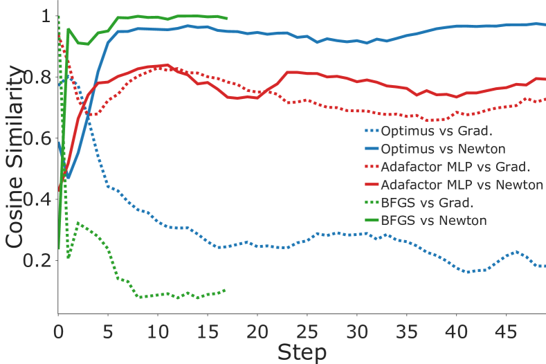
Figure 5: Mean similarity between Optimus update step and gradient and Newton direction on the 2d Rosenbrock function, averaged over 64 trajectories.

Results. We observe that Optimus typically converges to a lower objective value compared to other optimizers (see fig. 1 and supplementary material). We use the performance profile metric [6] to aggregate these results across functions. Note that it is not meaningful to directly average the per-function minima since each function is scaled differently and so values of minima are not directly comparable. The performance profile metric tackles this issue by relating minima for each function to its global minima, which is known for all objective functions in our benchmark. The results are shown fig. 3. We observe that performance of Optimus is higher than other optimizers across all values of performance threshold indicating that on average Optimus gets closer to global minimum of each function compared to other optimizers.

In fig. 4 we show relative number of iterations Optimus needs to reach the same objective value as Adam, BFGS and Adafactor MLP optimizers. The target objective value in this evaluation is defined as average objective value achieved by the corresponding baseline after $100$ iterations. The y-axis in fig. 4 corresponds to ratio between number of iterations required by a baseline and number of iterations required by Optimus. Values on y-axis larger than $1$ indicate that Optimus required fewer iterations. The x-axis in fig. 4 is a percentile of the tasks in the benchmark. A particular point on the plot then tells us what percentage of the benchmark has a ratio between number of iterations greater or equal than a value on y axis at that point.

For example, we observe that for about $50\%$ of the tasks Optimus requires about $10\times$ fewer iterations than Adam and BFGS and about $5\times$ fewer iterations than Adafactor MLP. In fig. 4 we label the x-axis with names of the objective functions corresponding to each point on the curve comparing Optimus to BFGS. We observe that BFGS excels on simple convex objective functions such as “Sphere” or their noisy versions such as “Griewank”, where it can quickly converge to global minimum. However BFGS fails on more complex functions with multiple local minima such as “Ackley” or functions where minima is located in a flat elongated valley such as “Rosenbrock” or “Dixon-Price”.

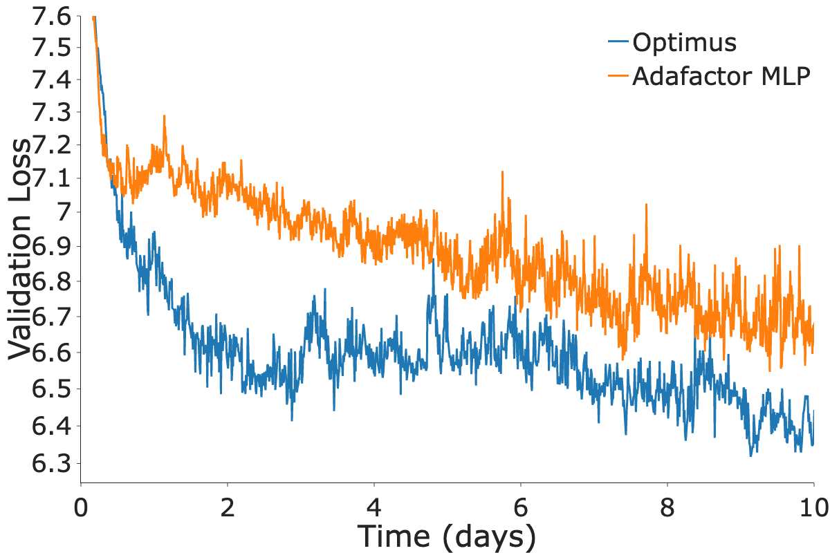
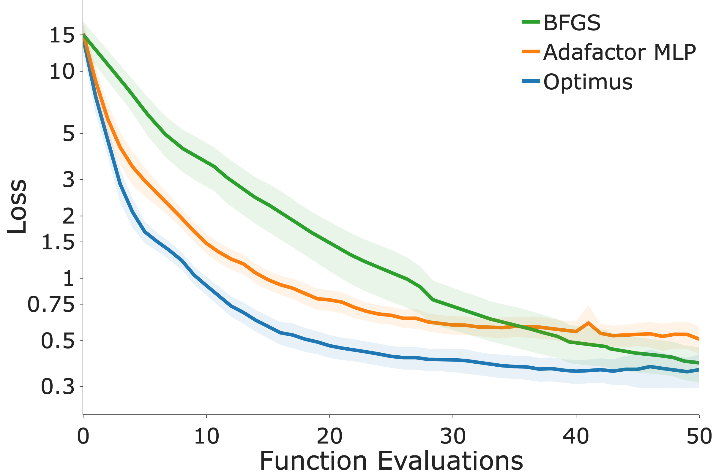
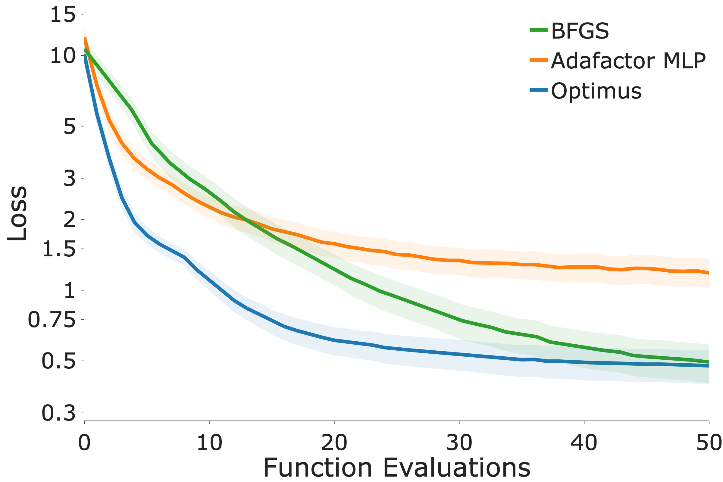
Figure 6: Left: comparison of validation loss during training of Optimus and Adafactor MLP. Note how Optimus converges to lower validation loss much faster than the Adafactor MLP model. Mid: comparison of loss curves during optimizing on “in domain” examples in tab. 1. Right: loss curves during optimizing of “out of domain” examples in tab. 1. Note how Optimus generalizes better than Adafactor MLP on out of domain data and minimizes the loss faster than BFGS. Shaded area denotes 95% confidence interval.

Method	MPJPE-G (in domain)	MPJPE-G (out of domain)	# Func. Evals
DiffPhy + BFGS  [15]	$38.3$	$24.7$	$71$
+ AdaFactor MLP [28]	$33.0$	$29.3$	$50$
+ Optimus (Ours)	$24.0$	$25.0$	$50$

Table 1: Comparison of different approaches to trajectory optimization on motion capture data from our Human3.6M validation set.

Analysis of update step direction. To further highlight differences between Optimus and Adafactor MLP  we plot the absolute cosine similarity of their step along the steepest descent direction given by $-\nabla{{\boldsymbol{\mathbf{x}}}}$, and the Newton direction given by $-{{\boldsymbol{\mathbf{H}}}}_{{{\boldsymbol{\mathbf{x}}}}}^{-1}\nabla{{\boldsymbol{\mathbf{x}}}}$, where ${{\boldsymbol{\mathbf{H}}}}_{{{\boldsymbol{\mathbf{x}}}}}^{-1}$ is the inverse Hessian at point ${{\boldsymbol{\mathbf{x}}}}$. The results are shown in fig. 5 for optimization of the 2d Rosenbrock function. For clarity we also include the same similarity plot for BFGS. As expected, the direction of BFGS step becomes similar to Newton after a few iterations since the preconditioner in BFGS approximates the inverse Hessian. Note that overall the direction of the Optimus step is much closer to Newton compared to Adafactor MLP  and much less similar to steepest descent. This supports the intuition that Optimus’s design extends the learned optimizer with a preconditioner similar to BFGS.

5.2 Physics-Based Motion Reconstruction

Model	MPJPE-G	MPJPE	MPJPE-PA	MPJPE-2d	TV	Foot skate
VIBE [20]	207.7	68.6	43.6	16.4	0.32	27.4
PhysCap [38]	-	97.4	65.1	-	-	-
SimPoE [53]	-	56.7	41.6	-	-	-
Shimada et al. [37]	-	76.5	58.2	-	-	-
Xie et al. [51]	-	68.1	-	-	-	-
DiffPhy [15]	139.1	82.1	55.9	13.2	0.21	7.2
Optimus (Ours)	138.6	82.8	57.0	13.2	0.20	6.5

Table 2: Quantitative results on Human3.6M [18] comparing our model to prior methods.

Model	MPJPE-G	MPJPE	MPJPE-PA	MPJPE-2d	TV	Foot skate
DiffPhy [15]	150.2	105.5	66.0	12.1	0.44	19.6
Optimus	149.8	104.4	66.4	12.1	0.45	21.5

Table 3: Quantitative results on generalizing to a new dataset. Optimus was trained Human3.6M [18] and is here evaluated on a subset of the dance motion dataset AIST [43].

Variant	MPJPE-G	Loss	# Params	Runtime (ms)
Optimus	33.1	0.534	832,526	78.9
Optimus, no state	36.5	0.675	832,526	115.1
Optimus, no structure	37.3	0.721	832,139	10.7
Adafactor MLP [28] 512x4	40.0	0.723	811,531	3.7
Adafactor MLP [28] 128x4	40.6	0.811	22,411	2.6
Optimus	33.1	0.534	832,526	78.9
Optimus, 50 iterations	28.5	0.383	832,526	78.9
Optimus + BasinHopping [47]	25.6	0.352	832,526	78.9

Table 4: Top: ablation of model components on motion capture from our Human3.6M [18] validation set. Bottom: comparison of different test time operating modes.

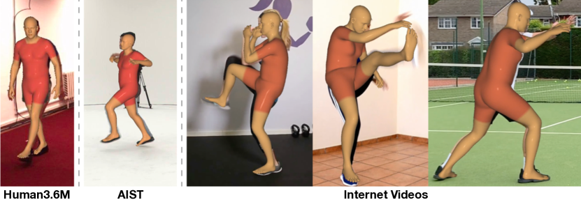
Figure 7: Qualitative examples of video reconstructions by Optimus. We train Optimus on the Human3.6M [18] dataset (left). We then evaluate its performance on the dancing sequence from AIST [43] (see tab. 3) and qualitatively verify that Optimus is applicable to in-the-wild internet videos (rightmost images).

In principle, learned optimization can be applied to any problem that is solvable by means of local descent, and thus to any physics-based reconstruction that formulates human motion reconstruction as loss minimization [23, 54, 15, 51]. In this paper, we build on the DiffPhy approach of [15], who define a differentiable loss function for physics-based reconstruction. DiffPhy relies on the differentiable implementation of rigid body dynamics in [16] and shape-specific body model based on [52] to define a loss function that measures similarity between simulated motion and observations. The observations are either a set of 3d keyframe poses, when the goal is to reproduce articulated 3d motion in physical simulation, or a sequence of image measurements such as 2d image keypoints or estimated 3d poses in each frame. The physical motion in DiffPhy is parameterized via a control trajectory, which is given by a sequence of quaternions defining a target rotation of each body joint over time. The control trajectory implicitly defines the torques applied to each body joint via PD-control. Please refer to [15] for a more extensive explanation of the loss function. Hence, optimization, in this case, aims to infer the control trajectory that re-creates an articulated motion in physical simulation in a way that is close to the given observations and consistent with constraints (e.g. lack of foot-skate and non-intersection with respect to a ground plane).

Datasets. In our human motion experiments, we use the popular Human3.6M articulated pose estimation benchmark [18]. We follow the protocol introduced in [38] to compare to related work for video-based experiments. For experiments with motion capture inputs, we rely the same subset of $20$ validation sequences from Human3.6M as used in [15]. We then additionally evaluate on the dancing sequences from the AIST dataset [43] used in [15] to further evaluate the generalization of our approach across qualitatively different motion types.

Evaluation metrics. We report the standard 2d and 3d human pose metrics as well as physics-based metrics. The mean per-joint 3d position error (MPJPE-G), the per-frame translation-aligned error (MPJPE), and the per-frame Procrustes-aligned error (MPJPE-PA) are reported in millimeters. In addition, we measure the 2d keypoint error of the reconstruction (MPJPE-2d) in pixels. Finally, we measure the amount of motion jitter as the total variation in 3d joint acceleration (TV) defined as $\frac{1}{T}\sum_{t\in T}\sum_{k\in K}|\ddot{x}^{k}_{t+1}-\ddot{x}^{k}_{t}|$, where $\ddot{x}^{k}_{t}$ is the 3d acceleration of joint $k$ at time $t$, as well as the percentage of frames exhibiting foot skate as defined by prior work [15].

Model training. We train Optimus and Adafactor MLP on the task of minimizing the DiffPhy loss, which measures similarity between the simulated motion and 3d poses estimated based on [55]. Following an initial grid-search to determine the best learning rate for each model, we train these for 10 days using 500 CPUs to generate training batches of optimization rollouts (128 roll-outs of length 50 per batch). We show loss vs. training time curves on the validation set in fig. 6 (left). Note that Optimus generally converges much faster and to a lower loss value compared to competitors. For example, after $48$ hours of training, Optimus has essentially converged to a loss of $6.49$ whereas Adafactor MLP requires nearly $240$ hours to reach a loss value of $6.55$.

Results. As our first experiment in tab. 1 we compare the performance of Optimus to Adafactor MLP and BFGS using motion capture (mocap) data as input. In fig. 6 (middle and right) we additionally visualize how quickly the loss is reduced by the optimizer at each iteration. Note that iterations of BFGS and of the learned optimizers are not comparable in terms of computational resources because BFGS might evaluate the objective function more than once during line search. To compensate for different iteration costs, in fig. 6 we plot the number of objective function evaluations instead of the optimization iteration along the x-axis. In this experiment we train all models on walking sequences from Human3.6M dataset . We refer to walking sequences as “in domain” in fig. 6 and tab. 1. We then assess performance on a validation set of “in domain” and “out of domain” sequences corresponding to motions other than walking. Note that Optimus improves over other approaches in the “in domain” setting and reaches the loss comparable to BFGS at roughly half of loss function evaluations (cf. fig. 6 (middle)). In the “out of domain” setting Optimus reaches nearly the same accuracy compared to BFGS ($24.7$ vs $25$mm.) but again converges much faster. In contrast Adafactor MLP does not improve over BFGS on the “out of domain” motions and converges to a higher loss (cf. fig. 6 (right)).

In the second experiment, we evaluate performance of our best model DiffPhy+Optimus for video-based human motion reconstruction. Note that Optimus performs well on the dancing sequences from AIST even though it has been trained only on walking data from Human3.6M ($150.2$ for DiffPhy vs. $149.8$ mm MPJPE-G for Optimus) and that Optimus is able to handle mocap and video inputs without retraining. We observe similar results on Human3.6M, where Optimus performs on par with BFGS ($138.6$ vs. $139.1$ MPJPE-G) while requiring roughly half as many function evaluations ($88$ for DiffPhy vs. $40$ for Optimus). We show a few qualitative examples for Optimus results on Human3.6M, AIST and internet videos in fig. 7.

Ablation experiments. We now evaluate how different design choices affect the model performance. Due to high computational load, we train each model for up to $48$ hours. The results are shown in tab. 4. We refer to a version of Optimus that does not incrementally update the matrix ${{\boldsymbol{\mathbf{B}}}}^{k}$ in sec. 4 and instead predicts it from scratch at each iteration as “Optimus, no state”, and a version that uses a transformer to directly predict $\Delta{{\boldsymbol{\mathbf{x}}}}^{k}$ from ${{\boldsymbol{\mathbf{s}}}}^{k}$ in Eq. 1 as “Optimus, no structure”. Our full Optimus improves over Adafactor MLP by $17.2\%$ and over simpler “Optimus, no structure” by $11.3\%$ while having nearly the same number of parameters. Note that simply adding more parameters to Adafactor MLP barely improves results ($40.6$ vs. $40.0$mm MPJPE-G). Optimus makes $30.3$ function evaluations before optimization is terminated by the stopping criterion. In tab. 4 (bottom three lines) we evaluate the effect of running Optimus for a fixed number of $50$ function evaluation without stopping criterion and the effect of using even more costly BasinHopping [47] optimization that adds random perturbations after a fixed number of iterations (to improve global exploration) requiring $82.3$ function evaluations on average. We observe that running Optimus for longer leads to considerably improved results, at higher computational load ($33.1$ for Optimus vs. $25.6$ mm MPJPE-G for Optimus+BasinHopping).

6 Conclusion

We have introduced a learned optimizer, Optimus, based on an expressive architecture that can capture complex dependency updates in parameter space. Furthermore, we have demonstrated the effectiveness of Optimus for the real-world task of physics-based articulated 3D motion reconstruction as well as on a benchmark of classical optimization problems. While Optimus’s expressive architecture outperforms simpler methods such as Adafactor MLP, the expressiveness comes at an increased computational cost. As a result, Optimus is best suited for tasks where the loss function dominates the computational complexity of optimization (e.g., physics-based reconstruction) but might be less suited for applications where the computation of the loss function is fast (e.g. training neural networks). In future work, we hope to address this limitation by learning factorizations of the estimated prediction matrix.
Ethical Considerations. We aim to improve the realism and quality of human pose reconstruction by including physical constraints. By amortizing the computation through learning from past instances, we hope to reduce the long-term computational demand of these methods. We believe that our physical model’s level of detail (e.g. lack of photorealistic appearance) limits its applications in adverse tasks such as person identification or deepfakes. Furthermore, the model is inclusive in supporting a variety of body shapes and sizes, and their underlying physics.

Appendix

In this supplementary material, we include additional results and visualizations (Appendix A), describe details of our implementation of Optimus (Appendix B), list the input features (Appendix C), summarize the hyperparameters of our method (Appendix D) and include the details of the datasets used in the paper (Appendix E).

Appendix A Additional visualizations

The following section provides additional visualizations of the experiments in the main paper.

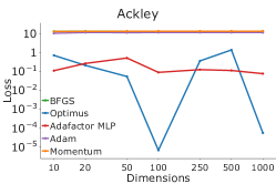
(a)

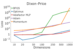
(b)

(c)

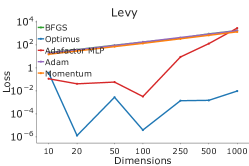
(d)

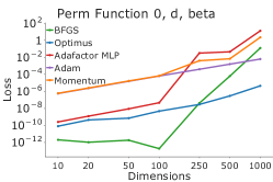
(e)

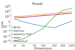
(f)

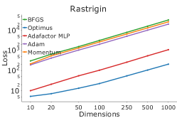
(g)

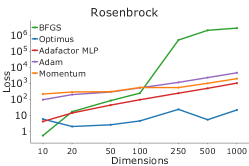
(h)

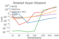
(i)

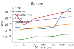
(j)

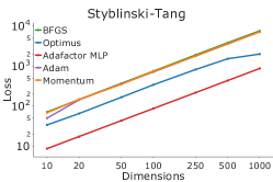
(k)

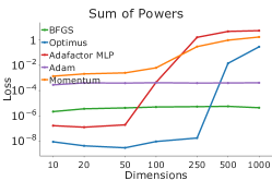
(l)

(m)

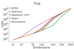
(n)

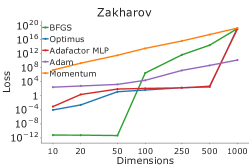
(o)

Figure 12: Evaluation results used to generate performance profile plot in Sec. 5.1 of the paper. Here we show results separately for each objective function. We plot objective value averaged over $64$ randomly initialized optimization runs on the y-axis and dimensionality of the objective function on the x-axis. Each method has a fixed budget of $200$ iterations.

Results on standard evaluation functions. We evaluate Optimus on a benchmark of 15 classical optimization test functions. figure 12 and LABEL:tab:full_classical_results provides detailed per-function results. These results were then aggregated to calculate the performance profile (fig. 3 in the main paper).

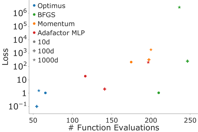
Figure 11: Comparison of loss vs number of function evaluations on the $N$-dimensional Rosenbrock functions for a maximum budget of $200$ steps. Note that BFGS may evaluate the function multiple times per step due to its line search.

Comparison of optimizer efficiency. figure 11 shows the efficiency of Optimus on $N$-dimensional Rosenbrock functions and compares it to other optimization algorithms. Note that Optimus achieves better loss values while using significantly less compute than BFGS and Adafactor MLP. For $N=1000$, Optimus converges after $\mathord{\sim}60$ function evaluations achieving a loss value $\mathord{\sim}5$ while BFGS achieves a loss of $\mathord{\sim}10^{6}$ using $\mathord{\sim}240$ function evaluations. The plot was generated using the same Rosenbrock optimization trajectories as presented in the main paper.

Runtime Comparison. In fig. 8 we plot the runtime of the optimization step for Optimus and other optimization methods on the task of finding minima of $N$-dimensional Rosenbrock functions while varying $N$ between $2$ and $1000$. In this comparison we use a widely adopted implementation of BFGS from the SciPy [46] package. Both Optimus and BFGS [14] have $\mathcal{O}(N^{2})$ time complexity. Interestingly for large $N$ Optimus optimization step is faster than BFGS, which is likely to be due to its more efficient Jax [10] implementation.

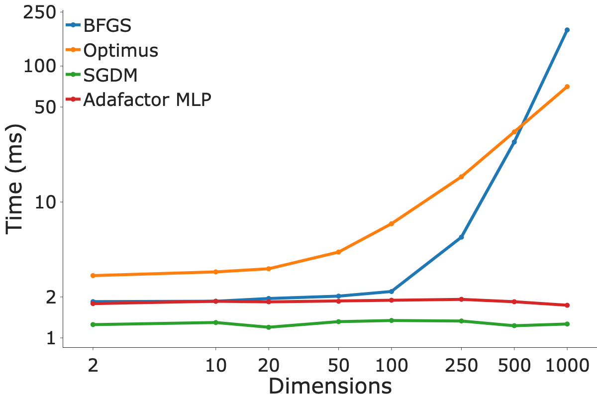
Figure 8: Time required to compute the optimizer update step as a function of dimensionality of the objective function.

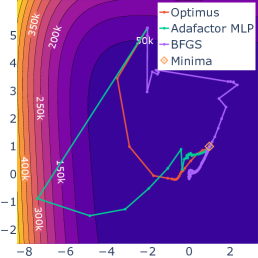
(a)

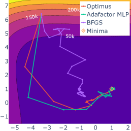
(b)

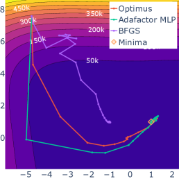
(c)

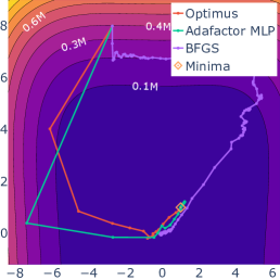
(d)

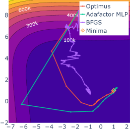
(e)

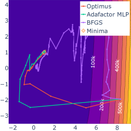
(f)

(g)

(h)

(i)

Figure 13: Example trajectories on $N$-dimensional Rosenbrock functions. We visualize the trajectory for the first two dimensions.

Additional Optimization Trajectories. figure 13 presents additional visualizations of optimization trajectories on $N$-dimensional Rosenbrock functions. Note how Optimus tends to vary its step size throughout the trajectories while Adafactor MLP tends to monotonically decrease its step size. We have observed that Adafactor MLP generally tends to learn a learning rate schedule based on the current iteration (a feature to the networks) and decrease its step size monotonically.

Appendix B Implementation details

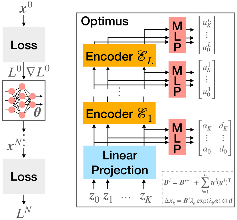
Figure 9: Left: schematic overview of applying our Transformer-based learned optimizer, Optimus, to iteratively minimize the loss $L$. Right: architecture of Optimus consisting of $L$ stacked Transformer encoders that predict the parameter update $\Delta{{\boldsymbol{\mathbf{x}}}}_{k}$ given the feature vector ${{\boldsymbol{\mathbf{z}}}}_{k}$ consisting of the associated gradient $\frac{dL}{d{{\boldsymbol{\mathbf{x}}}}_{k}}$ together with the features from [28].

The Optimus algorithm is shown in alg. 1 and the corresponding neural network architecture is shown in fig. 9.

Training. We implement Optimus in Jax [10] using Haiku [17] and the learned_optimization framework. When training Optimus on human motion reconstruction task we using a batch size of $20$. We generate the batches by sampling random windows from the Human3.6M [18] training set, then rolling out the optimization for $50$ steps, and computing the PES [45] gradients every $5$ steps using $2$ antithetic samples. We learn the weights using Adam [19] with the learning rate of $5\times 10^{-4}$. To stabilize the training we perform gradient clipping to gradients with a norm greater than $3$.

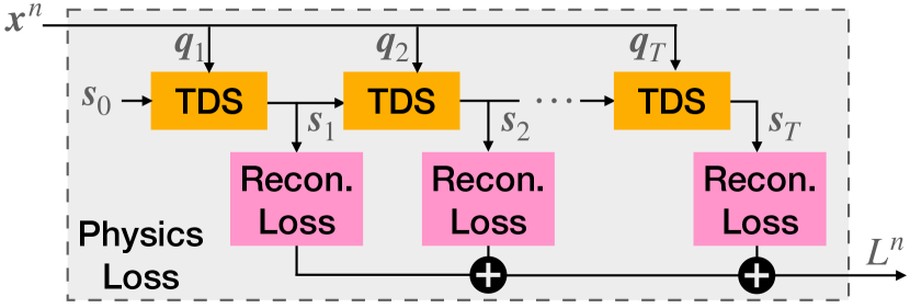
Figure 10: Overview of the physics loss introduced in [15] where the optimization variable ${{\boldsymbol{\mathbf{x}}}}$ corresponds to joint torques of a physically simulated human with the goal of minimizing a pose reconstruction loss between the physical character and observed visual evidence.

B.1 Distributed Physics Loss

We use the differentiable physics loss introduced in [15] using the Tiny Differentiable Simulator [16] (TDS) that was implemented in C++. A schematic overview of the loss function is available in fig. 10, however, see [15] for an in-depth explanation. The gradients of the loss are computed using the automatic differentiation framework CppAD [7]. We wrap the simulation step function as a custom TensorFlow [1] function to enable easier integration with Jax when training Optimus. We sample rollouts from $400$ distributed servers exposing the loss function using the Courier framework. We do this to overcome the issue of the slow evaluation time of the physics loss.

Appendix C Input features

In the following we list the features ${{\boldsymbol{\mathbf{z}}}}$ used as input by Optimus. The features are identical to the features used in [28] and we list them here to make the paper more self-contained.

• the parameter values

• the 3 momentum values ($m$)

• the second moment value ($v$)

• 3 values consisting of momenta normalized by rms gradient norm $-m/\sqrt{v}$

• the $(\sqrt{v+\epsilon})^{-1}$

• 3 AdaFactor normalized gradient values

• the tiled, AdaFactor row features (3 features)

• the tiled, AdaFactor column features (3 features)

• $1.0$ divided by the square root of these previous $6$ AdaFactor features

• 3 features consisting AdaFactor normalized momentum values

• 11 features formed by taking the current timestep, $t$, and computing $\mbox{tanh}(t/x)$ where $x\in\{1,3,10,30,100,300,1000,3000,10k,30k,100k\}$.

Appendix D Hyperparameters and Computional Resources

We train Optimus using a distributed setup on the Google Compute Engine. When training on the DiffPhy [15] reconstruction task, we distributed the loss function on $400$ vCPU instances. This significant computational cost is what motivated us to find a model which converges faster than prior work (e.g. Adafactor MLP [28]). We trained approximately $30$ such models throughout experimentation.

Training models on $N$-dimensional Rosenbrock functions was much faster as its loss function evaluates in $\mathord{\sim}5$ms rather than $\mathord{\sim}4$s. We trained those models for $48$ hours using $40$ vCPU instances. In total, we trained approximately $100$ such models.

The primary hyperparameters and the ranges of them that we tested are presented in tab. 7. Due to the high computational expense, we could not test all combinations exhaustively. We chose a short truncation length ($5$) on the physics tasks as it allows us to update the network more often which speed up the training convergence. Similarly, having a smaller batch size allowed us to update the model more frequently as gathering training batches was faster.

Sequence	Frames
gBR_sBM_c06_d06_mBR4_ch06	1-120
gBR_sBM_c07_d06_mBR4_ch02	1-120
gBR_sBM_c08_d05_mBR1_ch01	1-120
gBR_sFM_c03_d04_mBR0_ch01	1-120
gJB_sBM_c02_d09_mJB3_ch10	1-120
gKR_sBM_c09_d30_mKR5_ch05	1-120
gLH_sBM_c04_d18_mLH5_ch07	1-120
gLH_sBM_c07_d18_mLH4_ch03	1-120
gLH_sBM_c09_d17_mLH1_ch02	1-120
gLH_sFM_c03_d18_mLH0_ch15	1-120
gLO_sBM_c05_d14_mLO4_ch07	1-120
gLO_sBM_c07_d15_mLO4_ch09	1-120
gLO_sFM_c02_d15_mLO4_ch21	1-120
gMH_sBM_c01_d24_mMH3_ch02	1-120
gMH_sBM_c05_d24_mMH4_ch07	1-120

Table 5: Sequences from the dance dataset AIST [43] used for evaluation.

Appendix E Datasets Details

We use three sets of data in the paper. Firstly, we evaluate on the established Human3.6M [18] dataset, which is recorded in a laboratory setting with the permission of the actors. We list the sequences used in our validation set in tab. 6. When comparing to prior work we use the protocol established in [38] namely evaluating on sequences Directions, Discussions, Greeting, Posing, Purchases, Taking Photos, Waiting, Walking, Walking Dog and Walking Together from subjects S9 and S11. We evaluate the motions using only camera 60457274 and following prior work [38, 51] we downsample the sequences from $50$ FPS to $25$ FPS.

Next, we use the AIST [43] dataset which features professional dancers performing to copyright-cleared dance music. The sequences we evaluate on are given in tab. 5. Finally, we provide qualitative examples of our method on “in-the-wild“ internet videos that were released under creative common licenses.

Sequence	Subject	Camera Id	Frames
Phoning	S11	55011271	400-599
Posing_1	S11	58860488	400-599
Purchases	S11	60457274	400-599
SittingDown_1	S11	54138969	400-599
Smoking_1	S11	54138969	400-599
TakingPhoto_1	S11	54138969	400-599
Waiting_1	S11	58860488	400-599
WalkDog	S11	58860488	400-599
WalkTogether	S11	55011271	400-599
Walking_1	S11	55011271	400-599
Greeting_1	S9	54138969	400-599
Phoning_1	S9	54138969	400-599
Purchases	S9	60457274	400-599
SittingDown	S9	55011271	400-599
Smoking	S9	60457274	400-599
TakingPhoto	S9	60457274	400-599
Waiting	S9	60457274	400-599
WalkDog_1	S9	54138969	400-599
WalkTogether_1	S9	55011271	400-599
Walking	S9	58860488	400-599

Table 6: Sequences from the Human3.6M [18] pose dataset used in our ablations and experiments with reinforcement learning agents.

Initial guess $\mathbf{x}^{0}$

$\boldsymbol{B}^{0}\leftarrow\boldsymbol{I}$

$k\leftarrow 0$

repeat

     $\{{{\boldsymbol{\mathbf{\alpha}}}},{{\boldsymbol{\mathbf{d}}}},\Delta\boldsymbol{B}^{k}\}\leftarrow\text{Optimus}({{\boldsymbol{\mathbf{z}}}}^{k})$

     $\boldsymbol{B}^{k}\leftarrow\boldsymbol{B}^{k-1}+\Delta\boldsymbol{B}^{k}$ $\triangleright$ Update learned preconditioning matrix.

     $\mathbf{s}^{k}\leftarrow{{\boldsymbol{\mathbf{B}}}}^{k}[\lambda_{a}\exp(\lambda_{b}\boldsymbol{\alpha})\odot\mathbf{d}]$

     $\mathbf{x}^{k}\leftarrow\mathbf{x}^{k-1}+\mathbf{s}^{k}$

     $k\leftarrow k+1$

until $k>\text{MAX\_ITERS or}f({{\boldsymbol{\mathbf{x}}}}^{k})>\frac{1}{N}\sum_{i=1}^{N}\beta f({{\boldsymbol{\mathbf{x}}}}^{k-i})+\epsilon$

Algorithm 1 The Optimus algorithm. ${{\boldsymbol{\mathbf{z}}}}^{k}$ denotes the Adafactor MLP features from [28] and $\odot$ denotes elementwise multiplication.

Variable	Search grid	Value Used
Learning Rate	{0.1, 0.01, 0.001, $5\times 10^{-4}$, $1\times 10^{-4}$}	$5\times 10^{-4}$
Model Dimension	{64, 128, 256, 512}	128
# Encoders	{1, 2, 3, 4, 5}	3
$\lambda_{a}$	{0.001, 0.01, 0.1}	0.1
$\lambda_{b}$	{0.001, 0.01, 0.1}	0.1
Batch Size	{20, 50, 128}	20
PES truncation length	{5, 10, 20}	5

Table 7: An overview of the different hyperparameters tested during designing of Optimus. Value Used refers to the value used on the human pose reconstruction task from video.

Table 8: Full results for experiments on classical optimization functions. Each value is averaged over $64$ random initializations. We implement the functions according to the formulas presented in [41].

Function	BFGS	Optimus	Adafactor MLP	Adam	Momentum
Ackley 2d	1.11e+01	6.65e+00	1.69e-01	8.51e+00	8.99e+00
Ackley 10d	1.34e+01	7.16e-01	1.11e-01	1.06e+01	1.31e+01
Ackley 20d	1.36e+01	2.12e-01	2.68e-01	1.16e+01	1.34e+01
Ackley 50d	1.36e+01	5.46e-02	5.19e-01	1.15e+01	1.34e+01
Ackley 100d	1.37e+01	6.80e-06	9.02e-02	1.18e+01	1.36e+01
Ackley 250d	1.36e+01	3.65e-01	1.26e-01	1.18e+01	1.36e+01
Ackley 500d	1.37e+01	1.38e+00	1.13e-01	1.17e+01	1.37e+01
Ackley 1000d	1.37e+01	5.60e-05	7.71e-02	1.16e+01	1.37e+01
Dixon-Price 2d	4.64e-13	4.67e+00	8.86e-06	2.83e-01	5.42e+00
Dixon-Price 10d	6.35e-01	4.24e-01	6.67e-01	3.81e+00	2.49e+01
Dixon-Price 20d	6.67e-01	7.60e-03	6.68e-01	1.19e+01	3.44e+01
Dixon-Price 50d	7.58e-01	3.62e-02	6.77e-01	6.56e+01	8.19e+01
Dixon-Price 100d	5.54e+00	4.63e-01	7.20e-01	2.56e+02	1.89e+02
Dixon-Price 250d	8.67e+06	1.17e+00	1.05e+00	1.58e+03	9.12e+02
Dixon-Price 500d	8.93e+07	6.57e+00	2.20e+00	6.39e+03	6.60e+03
Dixon-Price 1000d	4.90e+08	3.30e+01	1.25e+01	2.53e+04	4.04e+09
Griwank 2d	2.00e-02	9.04e-01	1.43e-01	1.96e-02	1.91e-02
Griwank 10d	6.92e-02	2.81e-01	7.45e-01	5.16e-02	8.33e-02
Griwank 20d	5.78e-04	5.63e-02	8.05e-01	9.16e-03	8.78e-01
Griwank 50d	9.31e-10	4.48e-02	9.25e-01	1.62e-03	1.06e+00
Griwank 100d	0.00e+00	3.41e-02	1.79e+00	1.69e-03	1.11e+00
Griwank 250d	0.00e+00	4.68e-02	3.07e+00	9.31e-04	1.28e+00
Griwank 500d	0.00e+00	2.30e-02	5.20e+00	9.29e-04	1.57e+00
Griwank 1000d	0.00e+00	1.74e-01	9.34e+00	2.64e-04	2.14e+00
Levy 2d	8.36e+00	5.65e+00	3.74e+00	8.40e+00	3.80e+00
Levy 10d	2.20e+01	3.72e-01	1.15e-01	2.06e+01	1.53e+01
Levy 20d	4.00e+01	1.31e-06	4.16e-02	3.81e+01	3.03e+01
Levy 50d	9.51e+01	2.81e-03	5.89e-02	9.17e+01	7.12e+01
Levy 100d	1.83e+02	3.96e-06	3.27e-03	1.78e+02	1.37e+02
Levy 250d	4.20e+02	1.41e-03	8.96e+00	4.34e+02	3.39e+02
Levy 500d	9.28e+02	1.52e-03	1.31e+02	8.89e+02	6.95e+02
Levy 1000d	1.81e+03	9.78e-03	2.93e+03	1.76e+03	1.38e+03
Perm Function 0, d, beta 2d	1.76e-12	1.16e-01	1.07e-01	9.96e-09	5.65e-09
Perm Function 0, d, beta 10d	2.03e-12	8.17e-11	2.58e-10	5.69e-07	6.02e-07
Perm Function 0, d, beta 20d	1.06e-12	4.45e-10	1.24e-09	2.37e-06	2.60e-06
Perm Function 0, d, beta 50d	1.83e-12	7.14e-10	8.96e-09	1.61e-05	1.70e-05
Perm Function 0, d, beta 100d	1.89e-13	4.80e-09	4.70e-08	6.49e-05	6.73e-05
Perm Function 0, d, beta 250d	4.21e-08	2.95e-08	3.21e-02	4.02e-04	4.05e-03
Perm Function 0, d, beta 500d	6.24e-05	2.96e-07	4.53e-02	1.61e-03	6.86e-03
Perm Function 0, d, beta 1000d	1.25e-01	4.52e-06	1.33e+01	6.36e-03	2.27e+00
Powel 2d	1.08e-08	4.29e-01	5.16e+00	7.83e+00	3.43e+01
Powel 10d	1.81e-08	1.04e+01	7.02e+01	1.94e+01	1.20e+02
Powel 20d	1.15e-07	8.17e-01	5.39e+01	3.82e+01	1.50e+02
Powel 50d	2.09e-05	5.92e-02	1.14e+02	9.74e+01	4.31e+02
Powel 100d	1.78e-03	1.38e-02	2.94e+02	2.12e+02	8.98e+02
Powel 250d	9.41e+01	3.26e-03	5.87e+02	4.77e+02	2.18e+03
Powel 500d	3.35e+04	7.06e-02	1.37e+03	9.98e+02	4.54e+03
Powel 1000d	1.76e+05	1.26e+00	2.41e+03	1.93e+03	8.88e+03
Rastrigin 2d	6.17e+01	3.30e+00	2.85e+00	3.99e+01	5.59e+01
Rastrigin 10d	3.04e+02	5.24e+00	1.01e+01	1.93e+02	2.16e+02
Rastrigin 20d	6.57e+02	7.12e+00	2.10e+01	4.20e+02	5.44e+02
Rastrigin 50d	1.57e+03	1.33e+01	5.53e+01	1.05e+03	1.33e+03
Rastrigin 100d	3.18e+03	2.27e+01	1.05e+02	2.04e+03	2.66e+03
Rastrigin 250d	8.03e+03	5.48e+01	2.63e+02	5.14e+03	6.61e+03
Rastrigin 500d	1.61e+04	1.06e+02	5.45e+02	1.03e+04	1.33e+04
Rastrigin 1000d	3.30e+04	2.10e+02	1.10e+03	2.05e+04	2.67e+04
Rosenbrock 2d	5.07e-13	3.48e+01	5.06e-01	3.58e+00	5.17e+00
Rosenbrock 10d	5.43e-01	5.84e+00	4.12e+00	9.52e+01	2.16e+02
Rosenbrock 20d	1.69e+01	2.00e+00	1.41e+01	1.99e+02	2.89e+02
Rosenbrock 50d	8.40e+01	2.56e+00	4.40e+01	2.89e+02	3.04e+02
Rosenbrock 100d	2.46e+02	4.47e+00	9.50e+01	5.26e+02	5.56e+02
Rosenbrock 250d	5.24e+05	2.37e+01	2.45e+02	1.16e+03	5.50e+02
Rosenbrock 500d	2.11e+06	5.33e+00	4.93e+02	2.31e+03	1.02e+03
Rosenbrock 1000d	2.91e+06	2.17e+01	1.04e+03	4.61e+03	1.99e+03
Rotated Hyper-Ellipsoid 2d	2.36e-14	2.59e+01	1.74e+00	3.81e-07	5.32e-08
Rotated Hyper-Ellipsoid 10d	8.08e-15	2.18e+00	9.38e-03	2.31e-05	2.53e-05
Rotated Hyper-Ellipsoid 20d	1.45e-14	1.89e-01	6.46e-10	1.05e-04	9.07e-05
Rotated Hyper-Ellipsoid 50d	1.80e-15	1.95e-08	3.06e-07	6.81e-04	7.03e-04
Rotated Hyper-Ellipsoid 100d	7.18e-15	2.22e-07	2.24e+00	2.71e-03	2.86e-03
Rotated Hyper-Ellipsoid 250d	2.76e+02	5.88e-06	1.08e+01	1.71e-02	2.43e-01
Rotated Hyper-Ellipsoid 500d	4.09e+03	8.07e-05	7.24e+03	6.87e-02	3.61e+00
Rotated Hyper-Ellipsoid 1000d	1.91e+05	2.97e-04	3.70e+04	2.73e-01	1.94e+02
Sphere 2d	7.07e-14	4.24e-04	3.22e-03	1.84e-09	3.68e-11
Sphere 10d	1.25e-13	1.33e-09	1.81e-05	2.77e-08	1.66e-10
Sphere 20d	2.21e-13	7.14e-10	8.02e-09	6.15e-08	3.35e-10
Sphere 50d	1.40e-12	3.89e-10	7.48e-07	1.65e-07	8.28e-10
Sphere 100d	1.14e-12	5.59e-10	3.54e-06	3.32e-07	1.66e-09
Sphere 250d	1.73e-12	1.42e-09	2.19e-05	8.34e-07	4.13e-09
Sphere 500d	8.48e-12	4.04e-05	7.99e-05	1.68e-06	8.37e-09
Sphere 1000d	1.01e-11	1.60e-03	1.61e-04	3.33e-06	1.66e-08
Styblinski-Tang 2d	1.40e+01	4.59e+00	3.40e+00	1.10e+01	1.04e+01
Styblinski-Tang 10d	7.13e+01	3.39e+01	8.66e+00	5.00e+01	6.83e+01
Styblinski-Tang 20d	1.47e+02	6.51e+01	1.73e+01	1.43e+02	1.46e+02
Styblinski-Tang 50d	3.69e+02	1.66e+02	4.34e+01	3.61e+02	3.50e+02
Styblinski-Tang 100d	7.52e+02	3.40e+02	8.69e+01	7.10e+02	7.30e+02
Styblinski-Tang 250d	1.90e+03	8.20e+02	2.17e+02	1.78e+03	1.79e+03
Styblinski-Tang 500d	3.83e+03	1.52e+03	4.34e+02	3.57e+03	3.64e+03
Styblinski-Tang 1000d	7.59e+03	1.99e+03	8.70e+02	7.13e+03	7.17e+03
Sum of Powers 2d	3.86e-08	2.16e-08	3.42e-09	2.14e-06	3.96e-05
Sum of Powers 10d	2.16e-06	8.71e-09	1.66e-07	2.85e-04	1.38e-03
Sum of Powers 20d	3.60e-06	4.18e-09	1.25e-07	4.06e-04	2.11e-03
Sum of Powers 50d	4.24e-06	2.92e-09	1.92e-07	3.92e-04	2.53e-03
Sum of Powers 100d	4.99e-06	9.19e-09	4.53e-04	4.20e-04	6.37e-03
Sum of Powers 250d	5.32e-06	1.74e-08	1.66e+00	3.94e-04	3.05e-01
Sum of Powers 500d	5.63e-06	1.45e-02	4.90e+00	3.98e-04	9.88e-01
Sum of Powers 1000d	4.38e-06	2.95e-01	5.62e+00	4.14e-04	1.76e+00
Sum of Squares 2d	1.76e-12	1.16e-01	1.07e-01	9.96e-09	5.65e-09
Sum of Squares 10d	2.03e-12	8.17e-11	2.58e-10	5.69e-07	6.02e-07
Sum of Squares 20d	1.06e-12	4.45e-10	1.24e-09	2.37e-06	2.60e-06
Sum of Squares 50d	1.83e-12	7.56e-10	8.96e-09	1.61e-05	1.70e-05
Sum of Squares 100d	1.89e-13	4.80e-09	4.70e-08	6.49e-05	6.73e-05
Sum of Squares 250d	4.21e-08	2.95e-08	3.21e-02	4.02e-04	4.05e-03
Sum of Squares 500d	6.24e-05	2.96e-07	4.53e-02	1.61e-03	6.86e-03
Sum of Squares 1000d	1.25e-01	4.90e-06	1.33e+01	6.36e-03	2.27e+00
Trid 2d	5.00e+00	5.00e+00	5.00e+00	5.00e+00	5.00e+00
Trid 10d	6.50e+01	6.50e+01	6.51e+01	6.50e+01	6.50e+01
Trid 20d	2.30e+02	2.30e+02	2.31e+02	2.95e+02	2.30e+02
Trid 50d	1.33e+03	1.32e+03	1.35e+03	1.47e+04	1.32e+03
Trid 100d	5.16e+03	5.11e+03	1.39e+04	1.56e+05	1.04e+04
Trid 250d	5.55e+04	8.92e+05	2.18e+06	2.61e+06	1.57e+06
Trid 500d	4.67e+06	1.64e+07	2.09e+07	2.10e+07	1.83e+07
Trid 1000d	9.91e+07	1.57e+08	1.68e+08	1.67e+08	1.62e+08
Zakharov 2d	3.61e-12	2.21e-01	8.11e-05	1.58e-01	2.11e-02
Zakharov 10d	6.40e-12	9.58e-05	8.85e-04	3.00e+02	2.31e+07
Zakharov 20d	6.28e-12	2.61e-03	2.45e+00	6.68e+02	2.09e+09
Zakharov 50d	4.78e-12	1.46e+01	8.71e+01	1.83e+03	3.71e+11
Zakharov 100d	3.20e+06	4.54e+01	1.34e+02	2.71e+04	3.45e+13
Zakharov 250d	4.94e+11	2.12e+02	1.89e+02	1.81e+07	4.45e+15
Zakharov 500d	2.82e+14	3.46e+02	5.61e+02	4.80e+08	2.96e+17
Zakharov 1000d	1.53e+19	2.08e+19	1.15e+19	1.63e+10	2.08e+19

References

- [1] Martín Abadi, Ashish Agarwal, Paul Barham, Eugene Brevdo, Zhifeng Chen, Craig Citro, Greg S. Corrado, Andy Davis, Jeffrey Dean, Matthieu Devin, Sanjay Ghemawat, Ian Goodfellow, Andrew Harp, Geoffrey Irving, Michael Isard, Yangqing Jia, Rafal Jozefowicz, Lukasz Kaiser, Manjunath Kudlur, Josh Levenberg, Dandelion Mané, Rajat Monga, Sherry Moore, Derek Murray, Chris Olah, Mike Schuster, Jonathon Shlens, Benoit Steiner, Ilya Sutskever, Kunal Talwar, Paul Tucker, Vincent Vanhoucke, Vijay Vasudevan, Fernanda Viégas, Oriol Vinyals, Pete Warden, Martin Wattenberg, Martin Wicke, Yuan Yu, and Xiaoqiang Zheng. TensorFlow: Large-scale machine learning on heterogeneous systems, 2015. Software available from tensorflow.org.
- [2] D.H Ackley. A Connectionist Machine for Genetic Hillclimbing, volume SECS28. Kluwer Academic Publishers, Boston, 1987.
- [3] M Montaz Ali, Charoenchai Khompatraporn, and Zelda B Zabinsky. A numerical evaluation of several stochastic algorithms on selected continuous global optimization test problems. Journal of global optimization, 31(4):635–672, 2005.
- [4] Brandon Amos. Tutorial on amortized optimization for learning to optimize over continuous domains. arXiv preprint arXiv:2202.00665, 2022.
- [5] Marcin Andrychowicz, Misha Denil, Sergio Gomez, Matthew W Hoffman, David Pfau, Tom Schaul, and Nando de Freitas. Learning to learn by gradient descent by gradient descent. In Advances in Neural Information Processing Systems, pages 3981–3989, 2016.
- [6] Vahid Beiranvand, Warren Hare, and Yves Lucet. Best practices for comparing optimization algorithms. Optimization and Engineering, 18(4):815–848, 2017.
- [7] B. Bell. Cppad: a package for c++ algorithmic differentiation, 2021.
- [8] Samy Bengio, Yoshua Bengio, Jocelyn Cloutier, and Jan Gecsei. On the optimization of a synaptic learning rule. In Preprints Conf. Optimality in Artificial and Biological Neural Networks, pages 6–8. Univ. of Texas, 1992.
- [9] Yoshua Bengio, Samy Bengio, and Jocelyn Cloutier. Learning a synaptic learning rule. Université de Montréal, Département d’informatique et de recherche opérationnelle, 1990.
- [10] James Bradbury, Roy Frostig, Peter Hawkins, Matthew James Johnson, Chris Leary, Dougal Maclaurin, George Necula, Adam Paszke, Jake VanderPlas, Skye Wanderman-Milne, and Qiao Zhang. JAX: composable transformations of Python+NumPy programs, 2018.
- [11] Joao Carreira, Pulkit Agrawal, Katerina Fragkiadaki, and Jitendra Malik. Human pose estimation with iterative error feedback. In Proceedings of the IEEE conference on computer vision and pattern recognition, pages 4733–4742, 2016.
- [12] Tianlong Chen, Xiaohan Chen, Wuyang Chen, Howard Heaton, Jialin Liu, Zhangyang Wang, and Wotao Yin. Learning to optimize: A primer and a benchmark. arXiv preprint arXiv:2103.12828, 2021.
- [13] Elizabeth D Dolan and Jorge J Moré. Benchmarking optimization software with performance profiles. Mathematical programming, 91(2):201–213, 2002.
- [14] Roger Fletcher. Practical Methods of Optimization. John Wiley & Sons, New York, NY, USA, 1987.
- [15] Erik Gärtner, Mykhaylo Andriluka, Erwin Coumans, and Cristian Sminchisescu. Differentiable dynamics for articulated 3d human motion reconstruction. In Proceedings of the IEEE/CVF Conference on Computer Vision and Pattern Recognition, 2022.
- [16] Eric Heiden, David Millard, Erwin Coumans, Yizhou Sheng, and Gaurav S Sukhatme. NeuralSim: Augmenting differentiable simulators with neural networks. In Proceedings of the IEEE International Conference on Robotics and Automation (ICRA), 2021.
- [17] Tom Hennigan, Trevor Cai, Tamara Norman, and Igor Babuschkin. Haiku: Sonnet for JAX, 2020.
- [18] Catalin Ionescu, Dragos Papava, Vlad Olaru, and Cristian Sminchisescu. Human3.6m: Large scale datasets and predictive methods for 3d human sensing in natural environments. IEEE Transactions on Pattern Analysis and Machine Intelligence, 36(7):1325–1339, jul 2014.
- [19] Diederik P Kingma and Jimmy Ba. Adam: A method for stochastic optimization. arXiv preprint arXiv:1412.6980, 2014.
- [20] Muhammed Kocabas, Nikos Athanasiou, and Michael J. Black. Vibe: Video inference for human body pose and shape estimation. 2020 IEEE/CVF Conference on Computer Vision and Pattern Recognition (CVPR), Jun 2020.
- [21] Manuel Laguna and Rafael Martí. Experimental testing of advanced scatter search designs for global optimization of multimodal functions. Journal of Global Optimization, 33:235–255, 2005.
- [22] Ke Li and Jitendra Malik. Learning to optimize. In ICLR, 2017.
- [23] Zongmian Li, Jiri Sedlar, Justin Carpentier, Ivan Laptev, Nicolas Mansard, and Josef Sivic. Estimating 3d motion and forces of person-object interactions from monocular video. In Computer Vision and Pattern Recognition (CVPR), 2019.
- [24] James Lucas, Shengyang Sun, Richard Zemel, and Roger Grosse. Aggregated momentum: Stability through passive damping. arXiv preprint arXiv:1804.00325, 2018.
- [25] Dougal Maclaurin, David Duvenaud, and Ryan Adams. Gradient-based hyperparameter optimization through reversible learning. In International conference on machine learning, pages 2113–2122. PMLR, 2015.
- [26] Niru Maheswaranathan, David Sussillo, Luke Metz, Ruoxi Sun, and Jascha Sohl-Dickstein. Reverse engineering learned optimizers reveals known and novel mechanisms. In M. Ranzato, A. Beygelzimer, Y. Dauphin, P.S. Liang, and J. Wortman Vaughan, editors, Advances in Neural Information Processing Systems, volume 34, pages 19910–19922. Curran Associates, Inc., 2021.
- [27] Amil Merchant, Luke Metz, Samuel Schoenholz, and Ekin Dogus Cubuk. Learn2hop: Learned optimization on rough landscapes. In International Conference on Machine Learning, pages 8661–8671. PMLR, 2021.
- [28] Luke Metz, C Daniel Freeman, James Harrison, Niru Maheswaranathan, and Jascha Sohl-Dickstein. Practical tradeoffs between memory, compute, and performance in learned optimizers. arXiv preprint arXiv:2203.11860, 2022.
- [29] Luke Metz, C. Daniel Freeman, Samuel S. Schoenholz, and Tal Kachman. Gradients are not all you need, 2021.
- [30] Luke Metz, Niru Maheswaranathan, C Daniel Freeman, Ben Poole, and Jascha Sohl-Dickstein. Tasks, stability, architecture, and compute: Training more effective learned optimizers, and using them to train themselves. arXiv preprint arXiv:2009.11243, 2020.
- [31] Luke Metz, Niru Maheswaranathan, Jeremy Nixon, Daniel Freeman, and Jascha Sohl-Dickstein. Understanding and correcting pathologies in the training of learned optimizers. In International Conference on Machine Learning, pages 4556–4565, 2019.
- [32] H. Mühlenbein, M. Schomisch, and J. Born. The parallel genetic algorithm as function optimizer. 17(6–7):619–632, Sept. 1991.
- [33] Eunbyung Park and Junier B Oliva. Meta-curvature. Advances in Neural Information Processing Systems, 32, 2019.
- [34] Davis Rempe, Leonidas J. Guibas, Aaron Hertzmann, Bryan Russell, Ruben Villegas, and Jimei Yang. Contact and human dynamics from monocular video. In Proceedings of the European Conference on Computer Vision (ECCV), 2020.
- [35] H. H. Rosenbrock. An Automatic Method for Finding the Greatest or Least Value of a Function. The Computer Journal, 3(3):175–184, 01 1960.
- [36] Noam Shazeer and Mitchell Stern. Adafactor: Adaptive learning rates with sublinear memory cost. In International Conference on Machine Learning, pages 4596–4604. PMLR, 2018.
- [37] Soshi Shimada, Vladislav Golyanik, Weipeng Xu, Patrick P’erez, and Christian Theobalt. Neural monocular 3d human motion capture with physical awareness. ACM Transactions on Graphics (TOG), 40:1 – 15, 2021.
- [38] Soshi Shimada, Vladislav Golyanik, Weipeng Xu, and Christian Theobalt. Physcap: Physically plausible monocular 3d motion capture in real time. ACM Transactions on Graphics, 39(6), dec 2020.
- [39] Jie Song, Xu Chen, and Otmar Hilliges. Human body model fitting by learned gradient descent. In European Conference on Computer Vision, pages 744–760. Springer, 2020.
- [40] Roman Strongin and Yaroslav Sergeyev. Global Optimization with Non-Convex Constraints: Sequential and Parallel Algorithms. Springer US, New York, NY, USA, 2000.
- [41] S. Surjanovic and D. Bingham. Virtual library of simulation experiments: Test functions and datasets. Retrieved November 9, 2022, from http://www.sfu.ca/~ssurjano.
- [42] Tijmen Tieleman and Geoffrey Hinton. Lecture 6.5-rmsprop: Divide the gradient by a running average of its recent magnitude. COURSERA: Neural networks for machine learning, 4(2):26–31, 2012.
- [43] Shuhei Tsuchida, Satoru Fukayama, Masahiro Hamasaki, and Masataka Goto. Aist dance video database: Multi-genre, multi-dancer, and multi-camera database for dance information processing. In Proceedings of the 20th International Society for Music Information Retrieval Conference, ISMIR 2019, pages 501–510, Delft, Netherlands, Nov. 2019.
- [44] Ashish Vaswani, Noam Shazeer, Niki Parmar, Jakob Uszkoreit, Llion Jones, Aidan N Gomez, Łukasz Kaiser, and Illia Polosukhin. Attention is all you need. Advances in neural information processing systems, 30, 2017.
- [45] Paul Vicol, Luke Metz, and Jascha Sohl-Dickstein. Unbiased gradient estimation in unrolled computation graphs with persistent evolution strategies. In Marina Meila and Tong Zhang, editors, Proceedings of the 38th International Conference on Machine Learning, volume 139 of Proceedings of Machine Learning Research, pages 10553–10563. PMLR, 18–24 Jul 2021.
- [46] Pauli Virtanen, Ralf Gommers, Travis E. Oliphant, Matt Haberland, Tyler Reddy, David Cournapeau, Evgeni Burovski, Pearu Peterson, Warren Weckesser, Jonathan Bright, Stéfan J. van der Walt, Matthew Brett, Joshua Wilson, K. Jarrod Millman, Nikolay Mayorov, Andrew R. J. Nelson, Eric Jones, Robert Kern, Eric Larson, C J Carey, İlhan Polat, Yu Feng, Eric W. Moore, Jake VanderPlas, Denis Laxalde, Josef Perktold, Robert Cimrman, Ian Henriksen, E. A. Quintero, Charles R. Harris, Anne M. Archibald, Antônio H. Ribeiro, Fabian Pedregosa, Paul van Mulbregt, and SciPy 1.0 Contributors. SciPy 1.0: Fundamental Algorithms for Scientific Computing in Python. Nature Methods, 17:261–272, 2020.
- [47] David J. Wales and Jonathan P. K. Doye. Global optimization by basin-hopping and the lowest energy structures of lennard-jones clusters containing up to 110 atoms. The Journal of Physical Chemistry A, 101(28):5111–5116, 1997.
- [48] Paul J Werbos. Backpropagation through time: what it does and how to do it. Proceedings of the IEEE, 78(10):1550–1560, 1990.
- [49] Olga Wichrowska, Niru Maheswaranathan, Matthew W Hoffman, Sergio Gomez Colmenarejo, Misha Denil, Nando de Freitas, and Jascha Sohl-Dickstein. Learned optimizers that scale and generalize. International Conference on Machine Learning, 2017.
- [50] Yuhuai Wu, Mengye Ren, Renjie Liao, and Roger Grosse. Understanding short-horizon bias in stochastic meta-optimization. arXiv preprint arXiv:1803.02021, 2018.
- [51] Kevin Xie, Tingwu Wang, Umar Iqbal, Yunrong Guo, Sanja Fidler, and Florian Shkurti. Physics-based human motion estimation and synthesis from videos. In Proceedings of the IEEE/CVF International Conference on Computer Vision (ICCV), pages 11532–11541, October 2021.
- [52] Hongyi Xu, Eduard Gabriel Bazavan, Andrei Zanfir, William T Freeman, Rahul Sukthankar, and Cristian Sminchisescu. GHUM & GHUML: Generative 3d human shape and articulated pose models. In IEEE Conf. Comput. Vis. Pattern Recog., pages 6184–6193, 2020.
- [53] Ye Yuan, Shih-En Wei, Tomas Simon, Kris Kitani, and Jason Saragih. Simpoe: Simulated character control for 3d human pose estimation. In The IEEE/CVF Conference on Computer Vision and Pattern Recognition (CVPR), 2021.
- [54] Andrei Zanfir, Eduard Gabriel Bazavan, Hongyi Xu, Bill Freeman, Rahul Sukthankar, and Cristian Sminchisescu. Weakly supervised 3d human pose and shape reconstruction with normalizing flows. arXiv preprint arXiv:2003.10350, 2020.
- [55] Andrei Zanfir, Eduard Gabriel Bazavan, Mihai Zanfir, William T Freeman, Rahul Sukthankar, and Cristian Sminchisescu. Neural descent for visual 3d human pose and shape. 2021 IEEE/CVF Conference on Computer Vision and Pattern Recognition (CVPR), 2021.