On the Energy and Communication Efficiency Tradeoffs in Federated and Multi-Task Learning

Abstract

Recent advances in Federated Learning (FL) have paved the way towards the design of novel strategies for solving multiple learning tasks simultaneously, by leveraging cooperation among networked devices. Multi-Task Learning (MTL) exploits relevant commonalities across tasks to improve efficiency compared with traditional transfer learning approaches. By learning multiple tasks jointly, significant reduction in terms of energy footprints can be obtained. This article provides a first look into the energy costs of MTL processes driven by the Model-Agnostic Meta-Learning (MAML) paradigm and implemented in distributed wireless networks. The paper targets a clustered multi-task network setup where autonomous agents learn different but related tasks. The MTL process is carried out in two stages: the optimization of a meta-model that can be quickly adapted to learn new tasks, and a task-specific model adaptation stage where the learned meta-model is transferred to agents and tailored for a specific task. This work analyzes the main factors that influence the MTL energy balance by considering a multi-task Reinforcement Learning (RL) setup in a robotized environment. Results show that the MAML method can reduce the energy bill by at least $2\times$ compared with traditional approaches without inductive transfer. Moreover, it is shown that the optimal energy balance in wireless networks depends on uplink/downlink and sidelink communication efficiencies.

I Introduction

The underlying premise of Federated Learning (FL) is to train a distributed and privacy-preserving Machine Learning (ML) model for resource-constrained devices [1, 2, 3, 4]. Typically, FL requires frequent and intensive use of communication resources to exchange model parameters with the parameter server [5]. However, it is not optimized for incremental model (re)training and tracking changes in data distributions, or for learning new tasks, i.e., Multi-Task Learning (MTL). In particular, jointly learning new tasks using prior experience, and quickly adapting as more training data becomes available is a challenging problem in distributed ML and mission critical applications [6], a topic that still remains in its infancy [7].

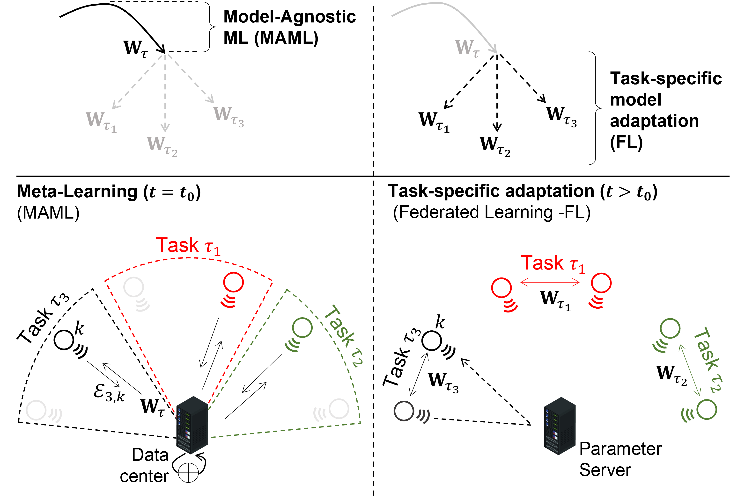
Figure 1: Clustered multi-task wireless network example. From left to right: Model-agnostic Meta-Learning (MAML) on the data center, and decentralized Federated Learning (FL) for task-specific model adaptation .

To obviate this problem, meta-learning is a promising enabler in multi-task settings as it exploits commonalities across tasks. In addition, meta-learning relies on the optimization of a ML meta-model that can be quickly adapted to learn new tasks from a small training dataset by utilizing few communication and computing resources (few shot learning) [8]. As depicted in Fig. 1, the meta-learning process requires an initial training stage ($t_{0}$ rounds) where a meta-model $\mathbf{W}_{\tau}$ is trained on a data center, using observations from different tasks, and fed back to devices (inductive transfer) for task-specific adaptations. The meta-model $\mathbf{W}_{\tau}$ could be quickly re-trained on the devices in a second stage ($t>t_{0}$), to learn a task-specific model $\mathbf{W}_{\tau_{i}}$, optimized to solve the (new) task $\tau_{i}$. Task-specific training of $\mathbf{W}_{\tau_{i}}$ can be implemented via FL using few communication resources and a small amount of data from the new task(s) [9]. Considering the popular Model-Agnostic Meta-Learning (MAML) algorithm [8], the meta-model $\mathbf{W}_{\tau}$ is optimized inside a data center using training data from a subset of devices (e.g., data producers such as sensors, machines and personal devices) and tasks. The meta-optimizer is typically gradient-based, and alternates task-specific model adaptations and meta-optimization stages on different data batches [10]. Although the optimization of the meta-model could be energy-hungry requiring more learning rounds than conventional ML on single tasks, the meta-learning process incurs lower energy consumption of subsequent task-specific model updates. Characterizing the tension between meta-model optimization and task-specific adaptation is currently overlooked and constitutes the focus of this work.

Contributions: this work provides a first look into the energy and communication footprints of meta-learning techniques implemented in distributed multi-task wireless networks. In particular, we consider a framework that quantifies the end-to-end energy cost of MAML optimization inside a data center, as well as the cost of subsequent task-specific model adaptations, implemented using FL [11, 12]. The work also includes, for the first time, comparisons and trade-off considerations about MAML-based optimization, and conventional transfer learning tools over resource-constrained devices. The framework is validated by targeting a multi-task Reinforcement Learning (RL) setup using real world data.

The paper is organized as follows. Sects. II and III describe the meta-learning approach, as well as its energy footprint evaluation, with a particular focus on communication and computing costs. In Sect. IV, we consider a case study in a real-world industrial workplace consisting of small networked robots collaboratively learning an optimized sequence of motions, to follow an assigned task/trajectory. Finally, Sect. V draws some conclusions.

II Multi-task learning and network model

The learning system under consideration consists of a clustered multi-task network of $K$ devices and one data center ($k=0$) co-located with a core network access point i.e, gateway, or Base Station (BS). The wireless network leverages UpLink (UL) and DownLink (DL) communication links with the data center (BS), or direct, i.e. sidelink (SL), communications. As depicted in Fig. 1, the devices, or agents, are allowed to cooperate with each other to learn $M\ll K$ distinct tasks $\tau_{1},...,\tau_{M}$ and form $M$ clusters $\mathcal{C}_{i}$ ($i=1,...,M$). The objective of the agents in the cluster $\mathcal{C}_{i}$ ($k\in\mathcal{C}_{i}$) is to learn a task $\tau_{i}$ by estimating the model parameters $\mathbf{W}_{\tau_{i}}$ through the minimization of a finite-sum objective function $\mathcal{L}_{i}(\mathbf{W})$ of the general form

$$\mathbf{W}_{\tau_{i}}=\underset{\mathbf{W}}{\mathrm{argmin}}\thinspace\mathcal{L}_{i}(\mathbf{W})=\underset{\mathbf{W}}{\mathrm{argmin}}\underset{\mathcal{L}_{i}(\mathbf{W})}{\underbrace{\sum_{k\in\mathcal{C}_{i}}L_{k}(\mathbf{W}|\mathcal{E}_{i,k})},}$$ (1)

where $L_{k}(\mathbf{W}|\mathcal{E}_{i,k})$ is the loss function, or cost, associated with the $k$-th device $L_{k}(\mathbf{W}|\mathcal{E}_{i,k})=\sum_{\mathbf{x}_{h,i}\in\mathcal{E}_{i,k}}\ell(\mathbf{W}|\mathbf{x}_{h,i})$, while $\ell(\mathbf{W}|\mathbf{x}_{h,i})$ is the loss function of the predicted model with data/examples $\mathbf{x}_{h,i}\in\mathcal{E}_{i,k}$ drawn from the task $\tau_{i}$. Notice that the costs of the individual devices belonging to the same cluster are minimized at the same location $\mathbf{W}_{\tau_{i}}$ as solving the same task $\tau_{i}$. However, considering two tasks $\tau_{i},\tau_{j}$ with $i\neq j$, it is $\mathbf{W}_{\tau_{i}}$ $\neq\mathbf{W}_{\tau_{j}}$. As clarified in the next section, the devices operate in a streaming data setting targeting a RL problem: each agent $k$ observes the environment at each time instant $t$ and obtains samples about the state, actions and task-dependent rewards.

The minimization of (1) is implemented incrementally via gradient optimization. In particular, we adopt an inductive transfer learning approach [13]. First, we learn a meta-model $\mathbf{W}_{\tau}$ on the data center using examples drawn from a subset $\mathcal{Q_{\tau}}$ of $Q\leq M$ tasks $\tau_{i}\in\mathcal{Q_{\tau}}$. After $t_{0}$ MAML rounds [8], the meta-model $\mathbf{W}_{\tau}$ is transferred from the data center to all the individual devices and adapted to the specific task via FL [6]. Notice that FL is implemented separately by devices in each cluster: in other words, only the agents within the same cluster are allowed to share their local models to learn a task-specific global model $\mathbf{W}_{\tau_{i}}$. Both the optimization of the meta-model and the subsequent task-specific adaptation stages contribute to the energy cost that are addressed in Sect. III.

II-A Model-Agnostic Meta-Learning (MAML)

Meta-learning operates at a higher level of abstraction [10] compared with conventional supervised learning. It uses randomly sampled observations from different tasks to identify a single model $\mathbf{W}_{\tau}$ such that, once deployed, few training steps are needed to adapt the meta-model to the new task(s) of interest. As seen in Fig. 1, MAML is implemented at the server upon the collection of random data $\mathcal{E}_{i,k}$ from $Q$ training tasks $\tau_{i}\in\mathcal{Q_{\tau}}$ over the uplink. The meta-model is optimized as

$$\mathbf{W}_{\tau}=\underset{\mathbf{W}}{\mathrm{argmin}}\thinspace\sum_{\tau_{i}\in\mathcal{Q_{\tau}}}\mathcal{L}_{i}(\mathbf{W}),$$ (2)

and solved iteratively via gradient-based optimization over multiple meta-learning rounds (i.e., MAML rounds).

Each MAML round is divided into two phases, namely the task-specific training stage, followed by the meta-model update stage. During task-specific training stage, $Q$ model adaptations $\mathbf{\mathbf{\varphi}}_{t,\tau_{i}}$ are obtained for each training task $\tau_{i}\in\mathcal{Q_{\tau}}$ using a sub-set $\mathcal{E}_{i,k}^{(a)}$ of the training data $\mathcal{E}_{i,k}^{(a)}\subset\mathcal{E}_{i,k}$ and the Stochastic Gradient Descent (SGD) algorithm. For iteration $t>0$ with random initialization at $t=0$ and training task $\tau_{i}$ it is

$$\boldsymbol{\mathbf{\varphi}}_{t,\tau_{i}}=\mathbf{W}_{t,\tau}-\mu\times\sum_{k\in\mathcal{C}_{i}}\nabla_{\mathbf{W}_{t,\tau}}L_{k}(\mathbf{W}_{t,\tau}|\mathcal{E}_{i,k}^{(a)}),$$ (3)

where $\mu$ is the SGD step size while $\nabla_{\mathbf{W}_{t,\tau}}L_{k}$ is the gradient of the loss function in (1) w.r.t. the meta-model $\mathbf{W}_{t,\tau}$. The subsequent meta-model update stage obtains an improved meta-model $\mathbf{W}_{t+1,\tau}$ for the next iteration $t+1$ that is trained over the remaining samples $\mathcal{E}_{i,k}^{(b)}:=\mathcal{E}_{i,k}\setminus\mathcal{E}_{i,k}^{(a)}$ (validation samples),

$$\mathbf{W}_{t+1,\tau}=\mathbf{W}_{t,\tau}-\eta\times\sum_{i=1}^{Q}\sum_{k\in\mathcal{C}_{i}}\nabla_{\mathbf{W}_{t,\tau}}L_{k}\left[\boldsymbol{\mathbf{\varphi}}_{t,\tau_{i}}|\mathcal{E}_{i,k}^{(b)}\right].$$ (4)

Notice that the vector $\nabla_{\mathbf{W}_{t,\tau}}L_{k}\left[\boldsymbol{\mathbf{\varphi}}_{t,\tau_{i}}|\mathcal{E}_{i,k}^{(b)}\right]$ requires gradient-through-gradient operation thus increasing the computational costs [9]. In particular, it is

$$\nabla_{\mathbf{W}_{t,\tau}}L_{k}\left[\boldsymbol{\mathbf{\varphi}}_{t,\tau_{i}}|\mathcal{E}_{i,k}^{(b)}\right]=\mathbf{J}_{\mathbf{W}_{t,\tau}}\left[\boldsymbol{\mathbf{\varphi}}_{t,\tau_{i}}\right]\times\nabla_{\mathbf{\varphi}_{t,\tau_{i}}}L_{k}\left[\boldsymbol{\mathbf{\varphi}}_{t,\tau_{i}}|\mathcal{E}_{i,k}^{(b)}\right]$$ (5)

where $\mathbf{J}_{\mathbf{W}_{t,\tau}}\left[\boldsymbol{\mathbf{\varphi}}_{t,\tau_{i}}\right]$ is the Jacobian operator while $\boldsymbol{\mathbf{\varphi}}_{t,\tau_{i}}=\boldsymbol{\mathbf{\varphi}}_{t,\tau_{i}}(\mathbf{W}_{t,\tau})$ is defined in (3). First-order approximation of $\mathbf{J}_{\mathbf{W}_{t,\tau}}\left[\boldsymbol{\mathbf{\varphi}}_{t,\tau_{i}}\right]\approx\mathbf{I}$ is often used [8]; in this case, (5) simplifies as $\nabla_{\mathbf{W}_{t,\tau}}L_{k}\left[\boldsymbol{\mathbf{\varphi}}_{t,\tau_{i}}|\mathcal{E}_{i,k}^{(b)}\right]\approx\nabla_{\boldsymbol{\mathbf{\varphi}}_{t,\tau_{i}}}L_{k}\left[\boldsymbol{\mathbf{\varphi}}_{t,\tau_{i}}|\mathcal{E}_{i,k}^{(b)}\right]$.

In what follows, the meta-optimization (4) is implemented for $t_{0}$ MAML rounds $\mathbf{W}_{\tau}\cong\mathbf{W}_{t_{0},\tau}$. As analyzed in the following, the energy footprint of meta-optimization is primarily ruled by the number of rounds $t_{0}$ as well as the number of training tasks $Q$ chosen by the meta-optimizer.

II-B Task-specific adaptation via FL network

Model adaptation uses a decentralized FL implementation [6]. Each device $k$ hosts a model initialized at time $t=0$ using the meta-model $\mathbf{W}_{t_{0},\tau}$, therefore $\mathbf{W}_{0,\tau_{i}}^{(k)}=\mathbf{W}_{t_{0},\tau}$. The local model $\mathbf{W}_{t,\tau_{i}}^{(k)}$ is then updated on consecutive rounds $t>0$ using new data/examples $\mathcal{E}_{i,k}$ drawn from possible new tasks $\tau_{i}$ and then shared with neighbor devices to implement average consensus [21]. Defining $\mathcal{N}_{k,i}\subseteq\mathcal{C}_{i}$ as the set that contains $N$ neighbors of node $k\in\mathcal{C}_{i}$, at every new round ($t>0$) each k-th device updates the local model as

$$\mathbf{W}_{t+1,\tau_{i}}^{(k)}\leftarrow\mathbf{W}_{t,\tau_{i}}^{(k)}+\sum_{h\in\mathcal{N}_{k,i}}\sigma_{k,h}\cdot(\mathbf{W}_{t,\tau_{i}}^{(h)}-\mathbf{W}_{t,\tau_{i}}^{(k)}),$$ (6)

where the weights $\sigma_{k,h}=\left|\mathcal{E}_{i,h}\right|/\sum_{j\in\mathcal{N}_{k,i}}\left|\mathcal{E}_{i,j}\right|$, computed using the size of the data distributions $\left|\mathcal{E}_{i,h}\right|$ and $\left|\left\{\mathcal{E}_{i,j}\right\}_{j\in\mathcal{N}_{k,i}}\right|$, are defined as in [5]. The local model update and the consensus steps are repeated until $\mathbf{W}_{\tau_{i}}=\underset{t\rightarrow\infty}{\lim}\mathbf{W}_{t,\tau_{i}}^{(k)}$, $\forall k\in\mathcal{C}_{i}$, or a desired training accuracy is obtained.

II-C Reinforcement learning problem

In the following, we consider, as an experimental case study, a Deep Reinforcement Learning (DRL) problem and off-policy training: for task $\tau_{i}$, the training dataset $\mathcal{E}_{i,k}:=(\mathbf{x}_{h,i},y_{h,i},r_{h,i},\mathbf{x}_{h+1,i},y_{h+1,i},r_{h+1,i},...)$ contains state ($\mathbf{x}_{h,i}$), action ($y_{h,i}$), and reward ($r_{h,i}$) time-domain sequences, that generally depend on the chosen problem $\tau_{i}$ to be solved. A specific example is given in Sect. IV. In RL jargon, for each task $\tau_{i}$, the problem we tackle is to learn a policy $\widehat{y}_{h+1,i}=\pi_{i}(\mathbf{x}_{h,i})$ that chooses the best action $\widehat{y}_{h+1,i}$ to be taken at time $h+1$ given the observation $\mathbf{x}_{h,i}$ at time $h$. We implemented a Deep Q-Learning (DQL) method: therefore, the policy is made greedy with respect to an optimal action-value function [14] $q_{\pi_{i}}^{*}(\mathbf{x}_{h,i},y_{h,i})$, such that $\pi_{i}(\mathbf{x}_{h,i})\doteq\arg\max_{y}q_{\pi_{i}}^{*}(\mathbf{x}_{h,i},y)$. The function $q_{\pi_{i}}^{*}$ (Q-function) predicts the expected future rewards for each possible action using the observations $\mathbf{x}_{h,i}$ as inputs. The Q-function $q_{\pi_{i}}^{*}$ is parameterized by a Deep Neural Network (DNN) model $q_{\pi_{i}}(\mathbf{x}_{h,i},y_{h,i}|\mathbf{W}_{\tau_{i}})$ and learned to minimize the loss function

$$\ell(\mathbf{x}_{h,i}|\mathbf{W}_{\tau_{i}})=\left[r_{h,i}+\nu\max_{y}\left(\widetilde{q}_{\pi_{i}}\right)-q_{\pi_{i}}(\mathbf{x}_{h,i},y|\mathbf{W}_{\tau_{i}})\right]^{2},$$ (7)

according to the Bellman equation, with $\nu=0.99$ being the discount factor and $\widetilde{q}_{\pi_{i}}$ a target Q-function network according to the double learning implementation [15].

The meta-learning process obtains a meta-model $\mathbf{W}_{\tau}$, solution to (2), that best represents the optimal Q-function set $\left\{q_{\pi_{i}}^{*},\forall i\text{ s.t. }\tau_{i}\in\mathcal{Q_{\tau}}\right\}$. Next, the parameters $\mathbf{W}_{\tau}$ could be quickly adapted during the task-specific adaptation ($t>t_{0}$) to approximate a specific Q-function $q_{\pi_{i}}^{*}$ solving a (new or unvisited) task $\tau_{i}$, i.e.,$\tau_{i}\notin\mathcal{Q_{\tau}}$. Notice that, during the meta-optimization stages, the training data $\mathcal{E}_{i,k}$ for $Q$ selected tasks are moved to the data center at each round using UL communication. Instead, during task-specific adaptation, devices from the same cluster $\mathcal{C}_{i}$ implement decentralized FL and exchange the parameters $\mathbf{W}_{\tau_{i}}$ of their estimated Q-function, rather than the training sequences: the data-center is thus not involved since devices communicate via sidelinks. In what follows, the average running reward $R=\sum_{h}\nu^{h}r_{h,i}$ is chosen as the accuracy indicator for each task.

III Energy and communication footprint model

The total amount of energy consumed by the MTL process is broken down into computing and communication [5]. Both the data center ($k=0$) and the devices ($k>0$) contribute to the energy costs, although data center is used for meta-model optimization and inductive transfer only. The energy cost is modelled as a function of the energy $E_{k}^{(\mathrm{C})}$ required for SGD computation, and the energy $E_{k,h}^{(\mathrm{T})}$ per correctly received/transmitted bit over the wireless link ($k,h$). The cost also includes the power dissipated in the RF front-end, in the conversion, baseband processing and other transceiver stages [5]. In what follows, we compute the energy cost required for the optimization of the meta-model (ML) and the task-specific model adaptation (FL), considering $M$ tasks. Numerical examples are given in Sect. IV.

III-A Meta-learning and task-specific adaptation

Training of the meta-model $\mathbf{W}_{\tau}$ runs for $t_{0}$ rounds inside the data center $k=0$. For each round, the data center: i) collects new examples $\mathcal{E}_{i,k}$ from $Q$ training tasks; ii) obtains $Q$ model adaptations (3) using data batches $\mathcal{E}_{i,k}^{(a)}\subset\mathcal{E}_{i,k}$, and iii) updates the meta-model for a new round by computing $Q$ gradients (4) using batches $\mathcal{E}_{i,k}^{(b)}\subset\mathcal{E}_{i,k}$. In particular, the cost of a single gradient computation $E_{0}^{(\mathrm{C})}=P_{0}\cdot T_{0}$ on the data center depends on the GPU/CPU power consumption $P_{0}$ and the time span $T_{0}$ required for processing an individual batch of data. Defining $\mathrm{B}_{i}^{(a)}$ and $\mathrm{B}_{i}^{(b)}$ as the number of data batches from the training sets $\mathcal{E}_{i,k}^{(a)}$ and $\mathcal{E}_{i,k}^{(b)}$, respectively, the total, end-to-end, energy (in Joule [J]) spent by the MAML process is broken down into learning ($\mathrm{L}$) and communication ($\mathrm{C}$) costs

$$E_{\mathrm{ML}}(t_{0},Q)=E_{\mathrm{ML}}^{(\mathrm{L})}(t_{0},Q)+E_{\mathrm{ML}}^{(\mathrm{C})}(Q).$$ (8)

For $t_{0}$ rounds and $Q$ task examples, it is

$$\begin{array}[]{c}E_{\mathrm{ML}}^{(\mathrm{L})}(t_{0},Q)=\gamma\cdot t_{0}\cdot\sum_{i=1}^{Q}\sum_{k\in\mathcal{C}_{i}}\left[\mathrm{B}_{i}^{(a)}+\beta\mathrm{B}_{i}^{(b)}\right]E_{0}^{(\mathrm{C})}\\ E_{\mathrm{ML}}^{(\mathrm{C})}(Q)=t_{0}\sum_{i=1}^{Q}\sum_{k\in\mathcal{C}_{i}}b(\mathcal{E}_{i,k})E_{k,0}^{(\mathrm{T})}+\sum_{k=1}^{K}b(\mathbf{W})E_{0,k}^{(\mathrm{T})}\end{array}$$ (9)

where the sum $\sum_{k=1}^{Q}\sum_{k\in\mathcal{C}_{i}}\mathrm{B}_{i}^{(a)}E_{0}^{(\mathrm{C})}$ quantifies the energy bill for $Q$ task-specific adaptations in (3), $\beta\cdot\sum_{i=1}^{Q}\sum_{k\in\mathcal{C}_{i}}\mathrm{B}_{i}^{(b)}E_{0}^{(\mathrm{C})}$ accounts for the meta-model update, and $\beta\geq 1$ includes the cost of the Jacobian computation ($\beta=1$ is assumed under first-order approximation). $\gamma$ is the Power Usage Effectiveness (PUE) of the considered data center [18]. UL communication of training data $\mathcal{E}_{i,k}$ has cost $\sum_{i=1}^{Q}\sum_{k\in\mathcal{C}_{i}}b(\mathcal{E}_{i,k})E_{k,0}^{(\mathrm{T})}$ that scales with the data size $b(\mathcal{E}_{i,k})$. DL communication $\sum_{k=1}^{K}b(\mathbf{W})E_{0,k}^{(\mathrm{T})}$ is required to propagate the meta-model $\mathbf{W}_{t_{0},\tau}$ to all devices: $b(\mathbf{W})$ quantifies the size (in Byte) of the meta-model trainable layers.

Task-specific model adaptations ($t>t_{0}$) are implemented independently by the devices in each cluster $\mathcal{C}_{i}$ using the same meta-model $\mathbf{W}_{t_{0},\tau}$ as initialization and the FL network. The energy footprint for adaptation over the task $\tau_{i}$ ($i=1,...,M$) could be similarly broken down into learning and communication costs [5] as

$$E_{\mathrm{FL}}(t_{i})=E_{\mathrm{FL}}^{(\mathrm{L})}(t_{i})+E_{\mathrm{FL}}^{(\mathrm{C})}(t_{i})$$ (10)

with

$$\begin{array}[]{c}E_{\mathrm{FL}}^{(\mathrm{L})}(t_{i})=t_{i}\cdot\sum_{k\in\mathcal{C}_{i}}\mathrm{B}_{i}E_{k}^{(\mathrm{C})}\\ E_{\mathrm{FL}}^{(\mathrm{C})}(t_{i})=b(\mathbf{W})\left[t_{i}\cdot\sum_{k\in\mathcal{C}_{i}}\sum_{h\in\mathcal{N}_{k,i}}E_{k,h}^{(\mathrm{T})}\right].\end{array}\begin{aligned} \end{aligned}$$ (11)

$t_{i}$ is the required number of FL rounds to achieve the assigned average running reward $R$ for the corresponding task, and $\mathrm{B}_{i}$ is the number of data batches from the training set $\mathcal{E}_{i,k}$ (now collected for task-specific model adaptation). Notice that $E_{k,h}^{(\mathrm{T})}$ represent the energy spent for sidelink communication between device $k$ and device $h\in\mathcal{N}_{k,i}$ in the corresponding neighborhood. When sidelink communication is not available, direct communication can be replaced by UL and DL communications, namely $E_{k,h}^{(\mathrm{T})}=E_{k,0}^{(\mathrm{T})}+\gamma\cdot E_{0,h}^{(\mathrm{T})}$, where $\gamma$ is the PUE of the BS or router hardware (if any).

III-B Tradeoff analysis in energy-constrained networks

In what follows, we analyze the tradeoffs between meta-optimization at the server and task-specific adaptation on the devices targeting sustainable designs. As previously introduced, MAML requires high energy costs $E_{\mathrm{ML}}$ (8) for moving data over UL. On the other hand, it simplifies subsequent task-specific model adaptations, reducing the energy bill $E_{\mathrm{FL}}$ on the devices. Communication and computing costs constitute the key indicators for such optimal equilibrium: to simplify the analysis of (8)-(9) and (10)-(11), energy costs are expressed $\forall k$ as efficiencies (bit/Joule) for uplink $\mathrm{E}_{\mathrm{UL}}=1/E_{k,0}^{(\mathrm{T})}$, downlink $\mathrm{E}_{\mathrm{DL}}=1/E_{0,k}^{(\mathrm{T})}$, and sidelink $\mathrm{E}_{\mathrm{SL}}=1/E_{k,h}^{(\mathrm{T})}$ communications [5], as well as for computing (gradient per Joule or grad/J for short) on the data center $\mathrm{E}_{\mathrm{0}}=1/E_{0}^{(\mathrm{C})}$ and for each k-th devices $\mathrm{E}_{\mathrm{C}}=1/E_{k}^{(\mathrm{C})}$. The problem we tackle is the minimization of the total energy cost $\mathrm{E}$ required for the joint learning of $M$ tasks,

$$\mathrm{E}=E_{\mathrm{ML}}(t_{0},Q)+\sum_{i=1}^{M}E_{\mathrm{FL}}(t_{i}).$$ (12)

Besides communication and computing efficiencies, the energy budget (12) depends the required number of MAML rounds $t_{0}$ and the training tasks $Q$ chosen for meta-optimization, as well as on the final accuracy, namely the number $t_{i}$ of FL rounds implemented by the devices for task-specific refinements.

IV Application: deep reinforcement learning

The considered multitask DRL setting is depicted in Fig. 2(a). Here, the agents are low-payload crawling robots organized into clusters: the robots in each cluster can cooperate (via sidelink communications) to learn a specific task. In particular, each cluster $\mathcal{C}_{i}$ is made up of 2 robots that collaborate to learn an optimized sequence of motions (i.e., actions) to follow an assigned trajectory $\tau_{i}$, namely, the task. A robot in cluster $\mathcal{C}_{i}$ that follows the trajectory $\tau_{i}$ correctly has fulfilled the assigned task. To simplify the setup, the trajectories followed by robots in each cluster are chosen from $M=6$ pre-assigned ones, as shown in Fig. 2(b). All trajectories have visible commonalities, i.e. a common entry point, but with different exits (or paths to follow) and are all implemented inside the same environment.

The robots can independently explore the environment to collect training data, namely state-action-reward sequences $\mathcal{E}_{i,k}$. However, the motion control problem is simplified by forcing all robots to move in a 2D regular grid space consisting of $40$ landmark points. The action space ($y_{h,i}$) thus consists of $4$ motions: Forward (F), Backward (B), Left (L), and Right (R). While moving in the grid space, each robot collects state observations ($\mathbf{x}_{h,i}$) obtained from two on-board cameras, namely a standard RGB camera and a short-range Time Of Flight (TOF) one [22]. Table I summarizes the relevant parameters for energy consumption evaluation. The datasets used for the DRL process and the meta-learning system are found in [16]. Notice that the computing energy of the data center and the devices, namely $P_{k}$ and $\mathrm{\mathrm{E}_{\mathrm{C}}}$, are measured from the available hardware. On the other hand, we quantify the estimated energy costs of meta-learning and FL stages by varying the communication efficiencies $\mathrm{E}_{\mathrm{UL}},\mathrm{E}_{\mathrm{DL}},\mathrm{E}_{\mathrm{SL}}$. Since real consumptions may depend on the specific protocol implementation and be larger than the estimated ones, we will highlight the relative comparisons.

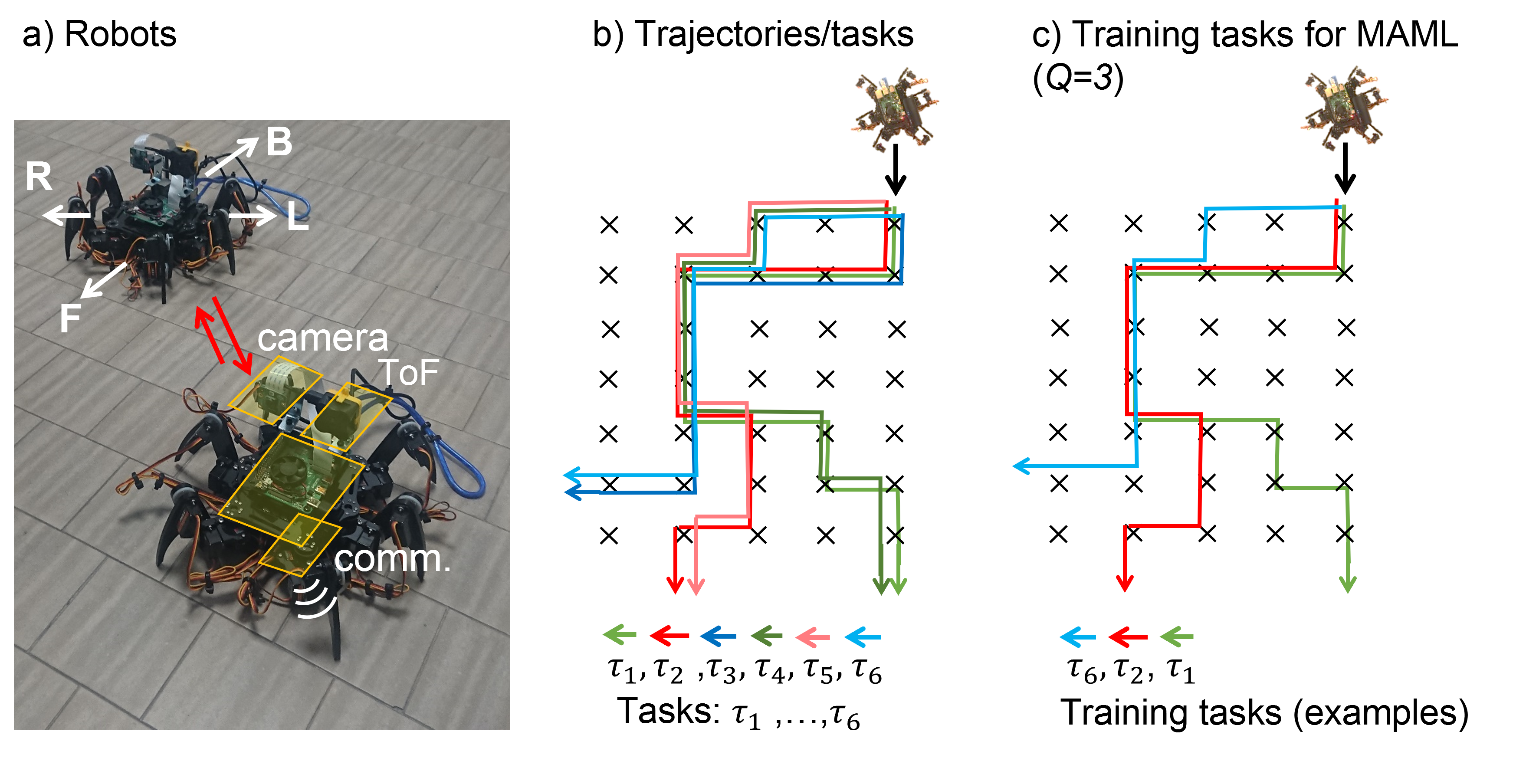
Figure 2: MTL case study. From left to right: (a) crawling robot deployment for data collection; (b) max-reward trajectories corresponding to the $M=6$ tasks; (c) trajectories/tasks used for MAML-based meta-model training.

TABLE I: Main system parameters for energy footprint evaluation on the data center (MAML) and on-devices (FL).

Parameters	Data center ($k=0$)	Devices ($k\geq 1$)
Comp. $P_{k}$:	$590\,\mathrm{W}$$\,\,(350\,\mathrm{W}$ GPU)	$5.1\,\mathrm{W}$ (CPU)
Batch time $T_{k}$:	$20\textrm{ ms}$	$400\textrm{ ms}$
Batches $B$:	$\mathrm{B}_{i}^{(a)},\mathrm{B}_{i}^{(b)}=10$	$\mathrm{B}_{i}=20$
Raw data size:	$Q\cdot b(\mathcal{E}_{i,k})$ MB	$b(\mathcal{E}_{i,k})\simeq 24.6$ MB
Model size:	$b(\mathbf{W})=5.6$ MB	$b(\mathbf{W})=5.6$ MB
PUE $\gamma$:	$1.67$	$1$
Comp. $\mathrm{\mathrm{E}_{\mathrm{C}}}$:	$0.03$ grad/J	$0.16$ grad/J

IV-A Multi-task learning and networking setup

Each task $\tau_{i}$ is described by a position-reward lookup table that assigns a reward value for each position in the 2D grid space, according to the assigned trajectory. Maximum reward trajectories for each of the $M=6$ tasks are detailed in Fig. 2(b). Note that robots get a larger reward whenever they approach the desired trajectory characterizing each task.

The DeepMind model [14] is here used to represent the parameterized Q-function $q_{\pi}(\mathbf{x},y|\mathbf{W})$ for DQL implementation: it consists of $5$ trainable layers, and $1.3$ M parameters with size $b(\mathbf{W})=5.6$ MB. The data center is remotely located w.r.t. the area where the robots are deployed so that communication is possible via cellular connectivity (UL/DL). The data center is equipped with a CPU (Intel i7 8700K, $3.7$ GHz) and a GPU (Nvidia Geforce RTX 3090, 24GB RAM). The robots mount a low-power ARM Cortex-A72 SoC and thus experience a larger batch time $T_{k}$, but a lower power $P_{k}$ as reported in Table I. In the following, we assume that the robots can exchange the model parameters via SL communication implemented by the WiFi IEEE 802.11ac protocol [23].

In each MAML round (described in Sect. II), the data center collects observations $\mathcal{E}_{i,k}$ for $Q=3$ training tasks ($\tau_{1},\tau_{2},\tau_{6}$), as depicted in Fig. 2(c). The training observations $\mathcal{E}_{i,k}:=(\mathbf{x}_{1,i},y_{1,i},r_{1,i},...,\mathbf{x}_{20,i},y_{20,i},r_{20,i})$ are obtained from $3$ robots and have size $b(\mathcal{E}_{i,k})\simeq 24.6$ MB as corresponding to $20$ consecutive robot motions (using an $\varepsilon$-greedy policy with $\varepsilon=0.1$). The training data are published to the data center via UL with efficiency $\mathrm{E}_{\mathrm{UL}}$ by using the MQTT transport protocol. The MQTT broker is co-located with the robots, while the data center retrieves the training sequences by subscribing to the broker. Task-specific adaptation via FL requires the robots in each cluster to mutually exchange the model parameters on each round using SL with efficiency $\mathrm{E}_{\mathrm{SL}}$. The MQTT payload is defined in [17] and includes: i) the local model parameters $\mathbf{W}_{t,\tau_{i}}^{(k)}$ that are binary encoded; ii) the corresponding task $\tau_{i}$ description; iii) the FL round $t_{i}$ or learning epoch; iv) the average running reward $R$. For all tasks, the number of FL rounds $t_{i}$ is selected to achieve the same average running reward of $R=50$ that corresponds to learned trajectories with Root Mean Squared Errors (RMSE) between $0.5$ m and $1$ m from the desired ones.

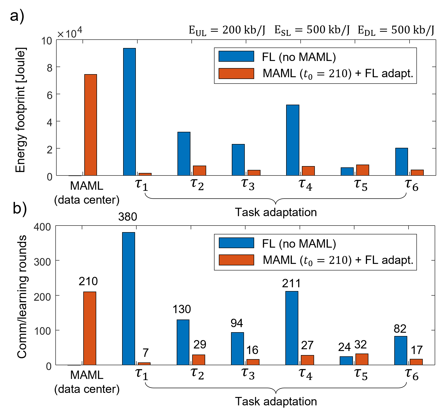
Figure 3: Energy footprints and communication/learning rounds. From top to bottom: (a) Energy footprint for MAML $E_{\mathrm{ML}}(t_{0})$, and subsequent task adaptations $E_{\mathrm{FL}}(t_{i})$, $i=1,...,6$ (orange bars), compared with FL without MAML (blue bars). (b) Communication and learning rounds required for MAML optimization ($t_{0}=210$ rounds on the data center) and for specific tasks $t_{i}$, $i=1,...,6$ (orange bars), compared with FL without MAML (blue bars). Note that the MAML energy cost per round in the data center (first bar from left to right) is higher than the one on the devices.

IV-B FL vs. MAML: energy, communication and learning rounds

Considering $M=6$ selected tasks, Fig. 3(a) shows the energy costs required for MAML optimization on the data center, and for the subsequent task-specific adaptations $\tau_{1},...,\tau_{6}$. Fig. 3(b) depicts the corresponding number of rounds ($t_{i}$) required to achieve the running reward of $R=50.$ Other learning parameters are defined in Table I. In particular, we consider a communication system characterized by $\mathrm{E}_{\mathrm{UL}}=200$ kb/J and $\mathrm{E}_{\mathrm{SL}}=500$ kb/J, in line with typical WiFi IEEE 802.11ac implementations [23, 24]. All results are considered by averaging over $15$ different Monte Carlo simulations using random model initializations (for both MAML meta-optimization and subsequent FL). For the considered MAML scenario (orange bars), the meta-model $\mathbf{W}_{t_{0},\tau}$ optimization runs on the data center for $t_{0}=210$ rounds. $\mathbf{W}_{t_{0},\tau}$ is then transferred to the robots for task adaptation using decentralized FL (6) over SL communications. In the same figure, the energy footprints and the learning rounds are compared to those obtained with a conventional approach (blue bars) where neither inductive transfer nor MAML are implemented, while tasks are learned independently by robots using decentralized FL [5] with local models randomly initialized (blue bars).

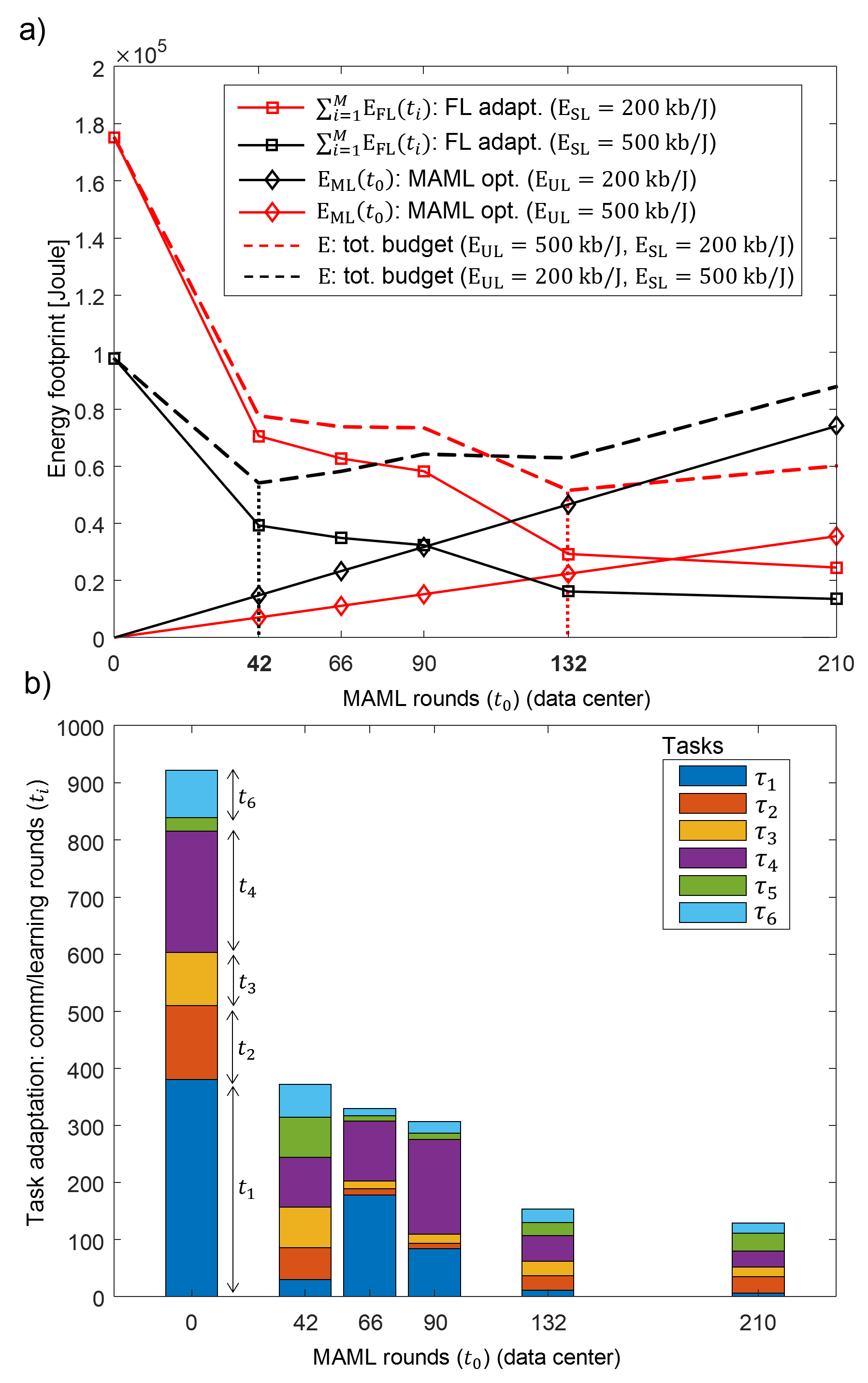
Figure 4: Impact of MAML rounds $t_{0}$ on MTL for varying communication efficiencies. From top to bottom: (a) impact of MAML rounds $t_{0}$ on the meta-learning energy $E_{\mathrm{ML}}$ (diamond markers), task adaptations $\sum_{i=1}^{M}E_{\mathrm{FL}}(t_{i})$ (squared markers), and total energy budget $\mathrm{E}$ in (12) in dashed lines. Black lines assumes D2D/mesh communications $\mathrm{E}_{\mathrm{SL}}=500$ kb/J more efficient than UL, $\mathrm{E}_{\mathrm{UL}}=200$ kb/J, while red lines assume the opposite. (b) impact of $t_{0}$ on the number of FL rounds $t_{i}$ required for task $\tau_{1},...,\tau_{6}$ adaptations.

MAML optimization is energy-hungry (with energy cost quantified as $E_{\mathrm{ML}}=74$ kJ) as it requires a significant use of UL resources for data collection over many learning rounds ($t_{0}=210$ in the example) to produce the meta-model. On the other hand, as reported in Fig. 3(b), task adaptations use few learning rounds/shots $t_{i}$ for model refinements, namely ranging from $t_{1}=7$ to $t_{5}=32$, reducing the robot energy footprints up to $10$ times for all tasks, i.e., $E_{\mathrm{FL}}(t_{1})=1.6$ kJ, and $E_{\mathrm{FL}}(t_{5})=7.9$ kJ. Decentralized FL without inductive transfer unloads the data center and requires marginal use of UL communication resources. However, considering the same tasks, it requires much more FL rounds (from $t_{5}=24$ to $t_{1}=380$) to converge compared with MAML approach. Interestingly, using MAML inductive transfer for learning of task/trajectory $\tau_{5}$ provides marginal benefits: this might be due to the fact that learning of the specific task $\tau_{5}$ marginally benefits from the knowledge of the meta-model. Overall, the total energy bill required to learn all the $6$ tasks through MAML and FL for subsequent task adaptation is quantified as $\mathrm{E}=E_{\mathrm{ML}}+\sum_{i=1}^{6}E_{\mathrm{FL}}(t_{i})=106$ kJ. This is approx. two times lower than the energy cost of learning each task separately using only FL with no inductive transfer $\mathrm{E}=\sum_{i=1}^{6}E_{\mathrm{FL}}(t_{i})=227$ kJ.

		FL rounds $t_{i}$ per tasks $\tau_{i}$, $i=1,..,6$
		$t_{1}$	$t_{2}$	$t_{3}$	$t_{4}$	$t_{5}$	$t_{6}$
MAML rounds	$t_{0}=0$	$380.1$	$129.6$	$93.7$	$211.5$	$24.2$	$82.4$
	(no MAML)
	$t_{0}=42$	$29.7$	$56.4$	$70.9$	$87$	$70.4$	$57.1$
	$t_{0}=66$	$178.8$	$9.9$	$14.3$	$104.6$	$9.8$	$12.4$
	$t_{0}=90$	$84.9$	$8.9$	$15.6$	$166.2$	$11.3$	$19.6$
	$t_{0}=132$	$11.6$	$25.5$	$25.1$	$44.6$	$23.1$	$23.8$
	$t_{0}=210$	$6.7$	$29.1$	$16.5$	$27.7$	$32$	$17.2$
	$t_{0}=240$	$2.7$	$10.8$	$9.1$	$40$	$21.8$	$19.6$

TABLE II: Average number of FL rounds $t_{i}$ for tasks $\tau_{1},...,\tau_{6}$, and varying $t_{0}$ as shown in Fig. 4(b). Average values w.r.t. 15 Monte Carlo runs.

IV-C MAML optimization and task adaptation tradeoffs

Balancing MAML optimization on the data center, with task-specific adaptations on the devices, is critical to improve efficiency. As analyzed previously, MAML requires an initial high energy cost for moving data on the UL over $t_{0}$ rounds; on the other hand, it simplifies subsequent task-specific model adaptations, reducing the energy bill for all tasks. Considering the same setting previously analyzed, Fig. 4 provides an in-depth analysis of MAML and FL tradeoffs, for varying communication efficiencies. In particular, in Fig. 4(a), we analyze the impact of MAML rounds $t_{0}$, namely the split point between the meta-model and task-specific adaptation, on the meta-learning energy cost $E_{\mathrm{ML}}$ (diamond markers), on the subsequent task adaptations $\sum_{i=1}^{M}E_{\mathrm{FL}}(t_{i})$ (squared markers), and on the total energy budget $\mathrm{E}$ (12) indicated in dashed lines. In Fig. 4(b) and Tab. II, we quantify the corresponding number of rounds $t_{i}$ required for task $\tau_{1},...,\tau_{6}$ adaptations and varying $t_{0}$. We consider varying number of MAML rounds, namely $t_{0}:=\left\{42,66,90,132,210,240\right\}$, each mapping onto a different number of SGD rounds for task-specific training (3) and meta-model update (4) stages implemented on the server.

In line with the results in Fig. 3, for the considered settings, the use of meta-learning ($t_{0}>0$) generally cuts the energy bill by least $2\times$ in all setups. Increasing the number of rounds $t_{0}$ on the data center improves the meta-model generalization capabilities and, as a result, reduces the energy cost (Fig. 4(a)) required for task adaptations $\sum_{i=1}^{M}E_{\mathrm{FL}}(t_{i})$ and the number of FL rounds $t_{i}$ (Fig. 4(b)). On the other hand, moving data on the cloud for many rounds increases the cost of MAML optimization $E_{\mathrm{ML}}$.

A judicious system design taking into account both MAML and task adaptation energy costs could bring significant energy savings. In Fig. 4(a) we thus highlight the optimal number of rounds $t_{0}$ required to minimize the total energy budget (12). Optimal MAML rounds depend on the uplink/sidelink communication costs: for example, when $\mathrm{E}_{\mathrm{SL}}=500$ kb/J and $\mathrm{E}_{\mathrm{UL}}=200$ kb/J (black lines), the number of MAML rounds should be limited to $t_{0}=42$, with $\mathrm{min_{\mathit{t_{\mathrm{0}}}}E}=56$ kJ. On the opposite, more efficient UL than SL communications, namely $\mathrm{E}_{\mathrm{UL}}=500$ kb/J and $\mathrm{E}_{\mathrm{SL}}=200$ kb/J (red lines), call for a larger number of MAML rounds ($t_{0}=132$) to reduce the FL costs with $\mathrm{min_{\mathit{t_{\mathrm{0}}}}E}=52$ kJ. Besides energy costs, Table II analyzes in more detail the impact of $t_{0}$ on the number of FL rounds/shots $t_{i}$ required for tasks $\tau_{1},...,\tau_{6}$ adaptations. The required rounds for task learning without inductive transfer ($t_{0}=0$) sum to $\sum_{i=1}^{L}t_{i}=910$ (Fig. 4(b)) and scale down up to $9$ times ($\sum_{i=1}^{L}t_{i}=103$) using $t_{0}$ MAML rounds on the data center. Notice that adaptations to new tasks $\left\{\tau_{3},\tau_{4},\tau_{5}\right\}\notin\mathcal{Q_{\tau}}$ not considered during meta-model training require (on average) more rounds $\sum_{i=3,4,5}t_{i}=70.9$ compared with previously trained tasks $\left\{\tau_{1},\tau_{2},\tau_{6}\right\}\in\mathcal{Q_{\tau}}$, $\sum_{i=1,2,6}t_{i}=33.1$.

V Conclusions

This work developed a novel framework for the energy footprint analysis of Model-Agnostic Meta-Learning (MAML) geared towards Multi-Task Learning (MTL) in wireless networks. The framework quantifies separately the end-to-end energy costs when using a data center for the MAML optimization, and the cost of subsequent task-specific model adaptations, implemented using decentralized Federated Learning (FL). We examined novel trade-offs about MAML optimization and few-shot learning over resource-constrained devices. The analysis was validated in a multi-task RL setup where robots collaborate to train an optimized sequence of motions to follow different trajectories, or tasks. For the considered MTL setup, MAML trains multiple tasks jointly and exploits task relationships to reduce the energy bill by at least two times compared with FL without inductive transfer. However, meta-learning requires moving data to the cloud for many rounds as well as larger computing costs. In many cases, the energy benefits of MAML also vary from task to task, suggesting the need of optimized MAML stages taking into account the specific commonalities among the tasks, including possible unseen ones. Finally, depending on communication efficiencies, a judicious design of the number of MAML rounds is critical to minimize the amount of data moved to the cloud. Communication and learning co-design principles are expected to further scale down the energy footprints.

References

- [1] P. Kairouz, et al., “Advances and open problems in federated learning,” Foundations and Trends in Machine Learning, Now Publishers, 2021. [Online]. Available: https://arxiv.org/abs/1912.04977.
- [2] T. Li, et al., “Federated learning: Challenges, methods, and future directions,” IEEE Signal Processing Magazine, vol. 37, no. 3, pp. 50–60, 2020.
- [3] M. Chen, et al., “Distributed learning in wireless networks: Recent progress and future challenges,” IEEE Journal on Selected Areas in Communications, vol. 39, no. 12, pp. 3579–3605, 2021.
- [4] M. M. Amiri, et al., “Federated learning over wireless fading channels,” IEEE Trans. Wireless Commun., vol. 19, no. 5, pp. 3546–3557, May 2020.
- [5] S. Savazzi, et al., “An Energy and Carbon Footprint Analysis of Distributed and Federated Learning,” IEEE Trans. on Green Communications and Networking, 2022, doi: 10.1109/TGCN.2022.3186439. [Online]. Available: https://arxiv.org/abs/2206.10380.
- [6] S. Savazzi et al., “Opportunities of Federated Learning in Connected, Cooperative and Automated Industrial Systems,” IEEE Communications Magazine, vol. 52, no. 2, February 2021.
- [7] J. Vanschoren, “Meta-learning”, in “Automated Machine Learning”, F. Hutter, L. Kotthoff, J. Vanschoren Editors, pp. 35–61, Springer, 2019.
- [8] C. Finn, et al., “Model-Agnostic Meta-Learning for Fast Adaptation of Deep Networks,” in Proc. 34th International Conference of Machine Learning (ICML), pp. 1126–1135, 2017.
- [9] A. Rajeswaran, et al., “Meta-Learning with Implicit Gradients,” in Proc. of 33rd Conference on Neural Information Processing Systems (NeurIPS), 2019.
- [10] O. Simeone, et al., “From Learning to Meta-Learning: Reduced Training Overhead and Complexity for Communication Systems,” 2020 2nd 6G Wireless Summit (6G SUMMIT), pp. 1-5, 2020.
- [11] X. Qiu, et al., “A first look into the carbon footprint of federated learning,” 2021. [Online]. Available: https://arxiv.org/abs/2102.07627M.
- [12] J. Konečný, et al. “Federated optimization: Distributed machine learning for on-device intelligence,” CoRR, 2016. [Online]. Available: http://arxiv.org/abs/ 1610.02527.
- [13] R. Nassif, et al., “Multitask Learning Over Graphs: An Approach for Distributed, Streaming Machine Learning,” IEEE Signal Processing Magazine, vol. 37, no. 3, pp. 14-25, May 2020.
- [14] V. Mnih, et al., “Human-level control through deep reinforcement learning,” Nature 518, pp. 529–533, 2015.
- [15] V. Van Hasselt, et al., “Deep reinforcement learning with double q-learning,” Proceedings of the AAAI conference on artificial intelligence. Vol. 30. No. 1. 2016.
- [16] Repository https://tinyurl.com/4wu3tbyb. Accessed: 5/4/2022.
- [17] B. Camajori Tedeschini, et al., “Decentralized Federated Learning for Healthcare Networks: A Case Study on Tumor Segmentation,” IEEE Access, vol. 10, pp. 8693-8708, 2022.
- [18] A. Capozzoli, et al., “Cooling systems in data centers: state of art and emerging technologies,” Energy Procedia, vol. 83, pp. 484–493, 2015.
- [19] David Lopez-Perez, et al., “A Survey on 5G Energy Efficiency: Massive MIMO, Lean Carrier Design, Sleep Modes, and Machine Learning,” 2021. [Online]. Available: https://arxiv.org/abs/2101.11246.
- [20] E. Björnson, et a., “How Energy-Efficient Can a Wireless Communication System Become?,” Proc. 52nd Asilomar Conf. on Sig., Syst., and Comp., Pacific Grove, CA, USA, 2018, pp. 1252–1256.
- [21] S. Savazzi, et al. “A Joint Decentralized Federated Learning and Communications Framework for Industrial Networks,” Proc. of IEEE CAMAD, Pisa, Italy, pp. 1–7, 2020.
- [22] Terabee, Teraranger EVO 64px, Technical Specifications, Terabee, 2018. [Online]. Available: https://tinyurl.com/vaz79xs. Accessed: Aug. 2021.
- [23] D. Camps-Mur, et al., “Enabling always on service discovery: Wifi neighbor awareness networking,” IEEE Wireless Communications, vol. 22, no. 2, pp. 118–125, April 2015.
- [24] David Lopez-Perez, et al., “A Survey on 5G Energy Efficiency: Massive MIMO, Lean Carrier Design, Sleep Modes, and Machine Learning,” 2021. [Online]. Available: https://arxiv.org/abs/2101.11246.