Empirical Asset Pricing via Ensemble Gaussian Process Regression

We introduce an ensemble learning method based on Gaussian Process Regression (GPR) for predicting conditional expected stock returns given stock-level and macro-economic information. Our ensemble learning approach significantly reduces the computational complexity inherent in GPR inference and lends itself to general online learning tasks. We conduct an empirical analysis on a large cross-section of US stocks from 1962 to 2016. We find that our method dominates existing machine learning models statistically and economically in terms of out-of-sample $R$-squared and Sharpe ratio of prediction-sorted portfolios. Exploiting the Bayesian nature of GPR, we introduce the mean-variance optimal portfolio with respect to the predictive uncertainty distribution of the expected stock returns. It appeals to an uncertainty averse investor and significantly dominates the equal- and value-weighted prediction-sorted portfolios, which outperform the S&P 500.

Keywords: empirical asset pricing, Gaussian process regression, portfolio selection, ensemble learning, machine learning, firm characteristics
JEL classification: C11, C14, C52, C55, G11, G12

1 Introduction

A central problem of empirical asset pricing is the prediction of conditional expected stock returns given the information set of market participants. Conditional expected returns are notoriously hard to predict, for a number of reasons. First, financial markets are very noisy and exhibit a low signal-to-noise ratio when compared to other domains such as computer vision, which is arguably due to the efficiency of the markets. Second, the full information set is not observable and likely too complex to model. The literature has accumulated a non-exhaustive list of predictive stock-level characteristics and macro-economic variables, which continuous to increase. Third, the relation between predictors and returns is evidently non-linear and time-varying due to the dynamically evolving economic conditions, which further complicates the problem.

Machine learning has the potential to accommodate a large number of features and a rich specification of functional forms, and is thus suited to the problem of predicting conditional expected returns. Interest in machine learning methods for empirical asset pricing has grown tremendously in academic finance and the industry. The leading example in this vein is Gu et al. (2020), who outline a new research agenda marrying machine learning with empirical asset pricing. They compare several machine learning methods for predicting stock returns, namely linear regression, generalized linear models with penalization, random forests, and neural networks. Other recent studies, such as Chen et al. (2022), Gu et al. (2021), further explore machine learning methods for empirical asset pricing, which are primarily based on neural networks. These articles provide empirical evidence that neural networks can significantly improve the predictive performance over traditional statistical methods and thus improve our empirical understanding of stock returns.

There are several points worthy of discussion in the above literature, which we will address in this paper. First, while neural networks have recently become the method of choice in many machine learning domains, such as computer vision, there are limitations to their application in finance. Neural networks thrive in data-rich environments. With many parameters to learn, they require massive training data and are computationally costly to train. Much of the literature on neural networks in empirical asset pricing focuses on monthly returns of a large cross-section of stocks spanning several decades. It is questionable whether neural networks would reasonably perform when restricted to smaller training sets, such as single industry sectors, or the S&P 500. Such samples only have a few thousand data points, which seems unsuitable for neural networks. What’s more, neural networks hardly adapt to online learning, so one has to re-train the whole network when new data arrives. In other words, neural networks are computationally intensive and hence not scalable in scenarios where data comes in sequentially, as with financial data. Second, the aforementioned articles do not address the uncertainty in the predictions based on their machine learning models. Quantifying uncertainty plays a significant role in finance when it comes to making decisions. Capturing uncertainties is crucial because the quality of our predictions directly impacts the quality of applications we build upon these predictions, for example, portfolio selection, hedging, or speculation. Third, while Gu et al. (2020) study generalized linear models with nonlinear transformations of the original features, they restrict these transformations to second order splines. As such they miss the full range of kernel ridge regression, which comes with a strong mathematical framework and constitutes a powerful machine learning method that works well on medium data sizes. Gaussian processes provide an alternative view on kernel ridge regression, by modeling a distribution over functions and performing inference directly in function space. This makes Gaussian process regression the method of choice when the quantification of prediction uncertainty is required, such as for financial decision making.

Our paper makes several methodological and empirical contributions that address the above points. First, we leverage kernel methods in machine learning, particularly Gaussian process regression (GPR), for predicting conditional expected stock returns given observable stock-level characteristics and macroeconomic variables. By doing so, we bridge the gap in Gu et al. (2020) and establish a link between two significant and growing research areas, kernel methods in machine learning and empirical asset pricing in financial economics. Thus, we contribute to the emerging literature on machine learning for empirical asset pricing.

Second, our empirical analysis confirms the insights from the growing literature that machine learning methods have excellent potential for predicting conditional expected returns. In particular, we show that a simple GPR model with very few hyper-parameters outperforms the leading benchmark model, both statistically and economically, in terms of out-of-sample $R$-squared and Sharpe ratio of prediction-sorted portfolios, respectively. We use the best prediction model based on neural networks in Gu et al. (2020) as the benchmark model in our analysis.

Third, a well-known issue with implementing GPR is the need to invert the kernel matrix repeatedly for the computation of the marginal log-likelihood function, which has a fundamental time complexity of the order $O(N^{3})$, where $N$ is the size of the training sample. This limitation prohibits, both in time and memory space, using GPR for large datasets. To tackle this computational bottleneck of GPR, we introduce an easy-to-implement ensemble learning method in the spirit of the mixture-of-experts approach. We thus also contribute to the literature on scalable GPR. Specifically, we partition the large training sample into subsets, apply individual GPRs on all subsets in parallel, and obtain a predictive distribution conditional on the full training data by mixing the predictive distributions over the subsets. Our ensemble approach offers several benefits: (i) it allows a straightforward parallel implementation of GPR on small training subsets, thus reducing the computational cost; (ii) it scales well with sample size and naturally lends itself to an online learning framework; and (iii) its data-driven mixing weight scheme takes into account the non-stationarity and heteroscedasticity present in the financial data.

Fourth, being a Bayesian method, the predictions from a GPR model come along with a predictive distribution. In particular, we obtain confidence intervals for the predicted conditional expected returns. As a novel application, we harness these uncertainty estimates. We find that incorporating uncertainty in portfolio construction leads to substantial statistical and economic improvements in terms of out-of-sample $R$-squared and Sharpe ratio of prediction-sorted portfolios, respectively. More precisely, we first use the predictive covariance matrix to construct a minimum uncertainty-weighted (UW) decile portfolio in the spirit of a global minimum variance portfolio. We find that the UW portfolio delivers a significantly high out-of-sample predictive pooled $R$-squared, $R_{pool}^{2}$, that outperforms the two traditional portfolios, namely, equal-weighted (EW) and value-weighted (VW). Motivated by this finding, we further exploit the predictive covariance matrix and introduce two new portfolios. The first is a prediction-weighted portfolio, originally proposed by Kaniel et al. (2022), which takes advantage of the ranking (to form decile portfolios) and the relative strengths of the predictions. The second is a prediction-uncertainty-weighted (PUW) portfolio in the spirit of the mean-variance optimal portfolio that gives more weight to stocks with higher predicted returns and minimizes uncertainty at the same time, which appeals to an uncertainty averse investor. We find that PW and PUW portfolios generate large economic gains, in terms of Sharpe ratio, compared to EW and VW portfolios.

We conduct an extensive empirical analysis, investigating monthly returns of a large cross-section of US stocks from 1962 to 2016. Our features include 94 time-varying stock-specific characteristics and their interactions with eight macroeconomic variables resulting in a feature vector of length 846. Our analysis shows that our model outperforms, out of sample, the leading benchmark approaches in predicting individual stock returns. In particular, our model generates an $R^{2}_{pool}$ of 1.29% compared to 0.4% for the neural network model in Gu et al. (2020) and 0.58% for the autoencoder model in Gu et al. (2021). We also evaluate the predictive performance of our model based on two alternative metrics. The first is the time-average of the monthly $R$-squared, $R^{2}_{avg}$, which gives equal weight to every month, in contrast to $R^{2}_{pool}$, which places more weight on months with larger cross-sections. The second is the information coefficient (IC), which quantifies the model’s ability to differentiate the relative performance among stocks disregarding the absolute levels of predictions. We find that $R^{2}_{avg}$ and IC are 0.7% and 9.7% for our model.

We also assess our model’s predictive performance at the portfolio level. In particular, we form decile portfolios (bottom $D1$ to top $D10$) sorted on out-of-sample stock return predictions from our model. Our UW portfolios achieve a higher $R$-squared than EW and VW portfolios for each decile. Further, when assessed over the grand panel of all decile portfolios, UW generates a $R_{pool}^{2}$ of 1.94% compared to -2.18% and -1.76% for EW and VW. The more pronounced predictive power of the UW portfolio shows that reducing prediction uncertainty is economically significant. We also find that the economic gains from the decile portfolios constructed using our predictions are large in terms of Sharpe ratio. For example, the PUW $D10$ portfolio yields an annualized out-of-sample Sharpe ratio of 1.447 compared to 1.392 (PW), 1.274 (EW), 1.042 (VW), and 0.36 of the S&P 500, which confirms that reducing prediction uncertainty matters economically. Our $D10$ portfolios also dominate the Sharpe ratios of 1.0 and 0.8 for the corresponding EW and VW $D10$ portfolios reported in Gu et al. (2020).

In sum, our paper confirms the great potential of machine learning for predicting conditional expected returns. We contribute to this understanding by adding prediction uncertainty, which greatly improves the performance of prediction-sorted portfolios. But machine learning methods on their own do not explain the statistical financial risk or underlying economic mechanisms. It remains a direction of future research to extend and add structure to our GPR approach, such as in Filipović and Pasricha (2022).

Our paper contributes to the fast emerging literature on machine learning for empirical asset pricing. In their pioneering work, Gu et al. (2020) conduct a comparative study of several machine learning methods to predict the grand panel of individual stock returns from the US markets and demonstrated the advantages of machine learning methods over traditional approaches. Similar studies are performed for European stock markets, Drobetz and Otto (2021), and bond markets, Bianchi et al. (2021). Gu et al. (2021) use an autoencoder neural network to demonstrate that imposing economic structure on a machine learning algorithm can substantially improve the estimation. In the same spirit, Chen et al. (2022) use deep neural networks with the fundamental no-arbitrage condition as a criterion function to estimate an asset pricing model for individual stock returns. These articles, however, exclude the important class of kernel-based models. We bridge this gap and show that our simple ensemble method based on GPR dominates the performance of their best benchmark models, which are based on neural networks. Our model leads to a better out-of-sample predictive $R$-squared, and further taking into account the estimates of the prediction accuracy leads to better portfolio performance in terms of Sharpe ratio.

The adoption of GPR in finance is only recent, albeit GPR has demonstrated much success outside of finance under the name of kriging. Williams and Rasmussen (2006) provide an extensive background on GPR models and highlight its applications in various fields. For instance, they emphasize that Gaussian processes can be viewed as a Bayesian non-parametric generalization of well-known econometrics techniques. In particular, a time series model, $AR(p)$, is a discrete-time equivalent of a Gaussian process model with Matérn covariance functions with an appropriate hyper-parameter choice. Han et al. (2016) combine Gaussian process state space models with stochastic volatility models and propose a GPR stochastic volatility (GPRSV) model to predict the volatility of the stocks returns. They also present an adjusted Markov Chain Monte Carlo to estimate their model and demonstrate, through empirical analysis, the superior predictive performance over the traditional GARCH and stochastic volatility models. De Spiegeleer et al. (2018) show how GPR can be deployed to approximate the derivative pricing function, for instance, pricing of exotic options under advanced models. They also study the application of GPR in the fitting of sophisticated Greek curves and implied volatility surfaces. Their numerical findings suggest that GPR could deliver a speed-up of a factor of several magnitudes relative to other benchmark methods for respective problems. Cousin et al. (2016) introduce shape-constrained Gaussian processes for yield-curve and credit default swaps (CDS) curve interpolation. Filipović et al. (2022b) and Filipović et al. (2022a) introduce an economically motivated kernel ridge regression method for estimating the yield and return curves of treasury bonds. Our paper seems to be the first that applies GPR to predicting conditional expected stock returns.

The paper is organized as follows. Section 2 introduces the model framework and our ensemble learning method based on GPR. Section 3 contains our empirical analysis. Section 4 concludes. Appendix A contains background material on Gaussian processes.

2 Methodology

Consider a financial market consisting of assets $i$ in discrete time $t=0,1,2,\ldots$, where $t$ represents the end of a month. More specifically, we denote by ${\mathcal{I}}_{t+1}$ the index set of assets $i$ that exist during the period $[t,t+1]$. At any time $t$, for any asset $i\in{\mathcal{I}}_{t+1}$, we observe the vector of predictor variables $x=x_{i,t}$ with values in a feature space $\mathcal{X}$ consisting of asset $i$-specific characteristics and common macro-economic variables.

We denote by $r_{i,t+1}$ the excess log return (henceforth simply referred to as “return”, if there is no risk of confusion) of asset $i$ over the period $[t,t+1]$. Following Gu et al. (2020), we describe it as an additive prediction error model,

$$r_{i,t+1}=E_{t}(r_{i,t+1})+\epsilon_{i,t+1},$$ (1)

where $E_{t}$ denotes the conditional expectation given the information available at time $t$. The errors $\epsilon_{i,t+1}$ are due to market imperfections and idiosyncratic noise. We assume that the conditional expected return is given by a common function $f:{\mathcal{X}}\to{\mathbb{R}}$,

$$E_{t}(r_{i,t+1})=f(x_{i,t}),\quad\text{for all $i\in{\mathcal{I}}_{t+1}$ and $t$.}$$ (2)

At any given time $t$, our goal is to learn $f$ from past data $\mathcal{D}=\{(x_{i,j-1},r_{i,j}),~{}i\in{\mathcal{I}}_{j},~{}j=1,2,\ldots,t\}$, and then predict next period conditional expected returns, $\hat{r}_{i,t+1}=f(x_{i,t})$, for $i\in{\mathcal{I}}_{t+1}$. We assume that the function $f$ does neither directly depend on the index $i$ nor time $t$, so that it can be learned efficiently using all instances in the panel data set $\mathcal{D}$.

2.1 Ensemble learning method based on Gaussian process regression

We use Gaussian process regression (GPR) to learn the function $f$ in (1) and (2). Thereto we assume that $f$ is a Gaussian process with some pre-specified prior mean function $m(\cdot)$ and covariance function, or, kernel $k(\cdot,\cdot)$. We assume that the errors $\epsilon_{i,t+1}$ are i.i.d. Gaussian random variables with mean 0 and variance $\sigma_{\epsilon}^{2}$ and independent of $f$. This means that the joint distribution of the past returns ${\bm{r}}_{1:t}=\{r_{i,j},~{}i\in{\mathcal{I}}_{j},~{}j=1,2,\ldots,t\}$ and the conditional expected returns $f({\bm{x}}_{t})=\{f(x_{i,t}),\ i\in{\mathcal{I}}_{t+1}\}$ is Gaussian of the form

$$\begin{pmatrix}{\bm{r}}_{1:t}\\ f({\bm{x}}_{t})\end{pmatrix}\sim{\mathcal{N}}\left(\begin{pmatrix}m({\bm{x}}_{0:t-1})\\ m({\bm{x}}_{t})\end{pmatrix},\begin{pmatrix}k({\bm{x}}_{0:t-1},{\bm{x}}_{0:t-1})+\sigma_{\epsilon}^{2}{I}&k({\bm{x}}_{0:t-1},{\bm{x}}_{t})\\ k({\bm{x}}_{t},{\bm{x}}_{0:t-1})&k({\bm{x}}_{t},{\bm{x}}_{t})\end{pmatrix}\right),$$ (3)

where ${I}$ is the identity matrix, and ${\bm{x}}_{0:t-1}=\{x_{i,j-1},~{}i\in{\mathcal{I}}_{j},~{}j=1,2,\ldots,t\}$ and ${\bm{x}}_{t}=\{x_{i,t},\ i\in{\mathcal{I}}_{t+1}\}$ denote the arrays of features observed by time $t-1$ and at $t$, respectively. Here, for a function $g:{\mathcal{X}}\to{\mathbb{R}}$ and an array $\bm{x}=\{x_{i}\}$ of points in ${\mathcal{X}}$, we denote by $g(\bm{x})=\{g(x_{i})\}$ the corresponding array of function values. In particular, $k({\bm{x}}_{0:t-1},{\bm{x}}_{0:t-1})$ is the $N\times N$ matrix of the covariances evaluated at all pairs of the past features ${\bm{x}}_{0:t-1}$, where $N=\sum_{j=1}^{t}|{\mathcal{I}}_{j}|$ denotes the size of the sample. Similarly, $k({\bm{x}}_{0:t-1},{\bm{x}}_{t})$ is the $N\times|{\mathcal{I}}_{t+1}|$ matrix of the covariances evaluated at all pairs of the past features ${\bm{x}}_{0:t-1}$ and current features ${\bm{x}}_{t}$.

The predictive (posterior) distribution of $f$ given the data $\mathcal{D}$ is again Gaussian with mean and covariance functions given by

$$\hat{m}(x) =m(x)+k(x,{\bm{x}}_{0:t-1})\left(k({\bm{x}}_{0:t-1},{\bm{x}}_{0:t-1})+\sigma_{\epsilon}^{2}{I}\right)^{-1}({\bm{r}}_{1:t}-m({\bm{x}}_{0:t-1})),$$ (4)

$$\hat{k}(x,x^{\prime}) =k(x,x^{\prime})-k(x,{\bm{x}}_{0:t-1})\left(k({\bm{x}}_{0:t-1},{\bm{x}}_{0:t-1})+\sigma_{\epsilon}^{2}{I}\right)^{-1}k({\bm{x}}_{0:t-1},x^{\prime}).$$ (5)

The mean $\hat{m}({{\bm{x}}_{t}})$ is then our prediction of the conditional expected return vector ${\bm{r}}_{t+1}$, and $\hat{k}({\bm{x}}_{t},{\bm{x}}_{t})$ represents the covariance of the Bayesian uncertainty of our prediction.

In our empirical analysis, we assume that errors $\epsilon_{i,t+1}$ are economically non-significant with a small fixed variance of $\sigma_{\epsilon}^{2}=10^{-10}$. This may seem at odds with the anecdotal low signal-to-noise ratio of stock returns. But we can argue that the Bayesian uncertainty of our predictor also adds noise to the signal, which here is the true conditional expected returns. On the other hand, adding $\sigma_{\epsilon}^{2}{I}$ to the kernel matrix $k({\bm{x}}_{0:t-1},{\bm{x}}_{0:t-1})$ has nevertheless a regularizing effect, as the latter may be ill-conditioned. We further set the prior mean function $m(\cdot)$ equal to zero. This is motivated by the empirical fact that zero predictions perform better than the historical mean of excess log returns, see Gu et al. (2020). Moreover, it is well documented in the literature that a zero prior mean usually works well for GPR, see De Spiegeleer et al. (2018); Williams and Rasmussen (2006).

The kernel $k(\cdot,\cdot)$ of the prior distribution of $f$ in (3) depends on hyper-parameters, which are estimated from the training data by maximizing the marginal log-likelihood, given by

$$\log p({\bm{r}}_{1:t}\mid{\bm{x}}_{0:t-1}) =-\frac{N\log(2\pi)}{2}-\frac{{\bm{r}}_{1:t}^{\top}\big{(}k({\bm{x}}_{0:t-1},{\bm{x}}_{0:t-1})+\sigma_{\epsilon}^{2}I\big{)}^{-1}{\bm{r}}_{1:t}}{2}$$ (6)

$$\quad-\frac{\log\det(k({\bm{x}}_{0:t-1},{\bm{x}}_{0:t-1})+\sigma_{\epsilon}^{2}I)}{2}.$$

A known challenge in GPR is that the computation of the log-likelihood function (6) involves repeated inversion of the regularized kernel matrix, which takes time of the order $O(N^{3})$. This is only feasible for a small $N$ (less than several thousand), which is not the case for the problem at hand for which $N$ is of the order of millions.

We tackle the computational bottleneck of GPR and introduce an ensemble approach in the spirit of the mixture-of-experts method. Thereto, we partition the training data into subsets, apply a GPR on each subset in parallel, and obtain a predictive distribution conditional on the full training data by mixing the predictive distributions over the subsets. In contrast to ad hoc partitioning schemes used in the literature, such as random or clustering based partitioning, we use that our training data is naturally divided into monthly subsets. That is, we treat data from each month $j=1,2,\ldots,t$ as a training subset on which we train an individual Gaussian process $f^{(j)}$. Specifically, we estimate hyper-parameters by maximizing the log-likelihood function (6), and obtain the predictive Gaussian distribution of $f^{(j)}$ with mean and covariance functions $\hat{m}^{(j)}(\cdot)$ and $\hat{k}^{(j)}(\cdot,\cdot)$ as in (4) and (5), with the training data $\{{\bm{x}}_{0:t-1},{\bm{r}}_{1:t}\}$ replaced by $\{{\bm{x}}_{j-1},{\bm{r}}_{j}\}$.

Finally, we obtain the predictive distribution conditional on the full training data by mixing the individual predictive Gaussian distributions of $f^{(j)}({\bm{x}}_{t})$ using some weights $w_{j}\geq 0$ with $\sum_{j}w_{j}=1$. The mean vector and covariance matrix of this Gaussian mixture distribution are given by

$$\hat{\bm{r}}_{t+1} =\sum_{j}w_{j}\hat{m}^{(j)}({\bm{x}}_{t}),$$ (7)

$$\hat{{\bm{\Sigma}}}_{t+1} =\sum_{j}w_{j}\hat{{\bm{M}}}^{(j)}_{t+1}-\hat{{\bm{r}}}_{t+1}\hat{{\bm{r}}}_{t+1}^{\top},$$ (8)

where $\hat{{\bm{M}}}^{(j)}_{t+1}=\hat{k}^{(j)}({\bm{x}}_{t},{\bm{x}}_{t})+\hat{m}^{(j)}({\bm{x}}_{t})\hat{m}^{(j)}({\bm{x}}_{t})^{\top}$ denotes the second order moment matrix of $f^{(j)}({\bm{x}}_{t})$. The mean $\hat{\bm{r}}_{t+1}$ is our ensemble prediction of the conditional expected return vector ${\bm{r}}_{t+1}$, and $\hat{{\bm{\Sigma}}}_{t+1}$ represents the covariance of the Bayesian uncertainty of our prediction.

For our empirical analysis, we implement the following two mixing weight schemes:

1. Equal weights: we select the $K_{t}\leq t$ most recent training months (more details on the choice of $K_{t}$ follow in the next subsection), set $w_{j}=0$ for $j\leq t-K_{t}$, and apply equal weights $w_{j}=1/K_{t}$ to the GPR models $j=t-K_{t}+1,\dots,\,t-1,\,t$. The sums in (7) and (8) are effectively over $j=t-K_{t}+1,\dots,\,t-1,\,t$.

2. MSE weights: as above we select the $K_{t}\leq t$ most recent training months and set $w_{j}=0$ for $j\leq t-K_{t}$. We also hold out the most recent training month, $w_{t}=0$, which we call calibration month, and define the weights for the remaining $K_{t}-1$ months as proportional to the mean squared error

   $$MSE_{j}=\frac{1}{|{\mathcal{I}}_{t}|}\sum_{i\in{\mathcal{I}}_{t}}(r_{i,t}-\hat{r}^{(j)}_{i,t})^{2},$$

   of GPR model $j$ on the calibration month $t$ with corresponding predicted returns $\hat{r}^{(j)}_{i,t}=\hat{m}^{(j)}(x_{i,t-1})$. The MSE weights are thus given by

   $$w_{j}=\frac{1/MSE_{j}}{\sum_{s=t-K_{t}+1}^{t-1}1/MSE_{s}},\quad j=t-K_{t}+1,\dots,t-2,\,t-1.$$

   That is, the smaller $MSE_{j}$ the larger the weight $w_{j}$ we give to GPR model $j$. The sums in (7) and (8) are effectively over $j=t-K_{t}+1,\dots,\,t-2,\,t-1$.

Our ensemble approach has several advantages. First, it offers a substantial computational speed-up, due to a straightforward parallel implementation of the individual GPR models on subsets of the training data, compared to training a GPR model on the full training data. Second, the flexibility that each GPR model can have its own set of optimal hyper-parameters (the parametric kernel is the same for each model) allows to account for the non-stationarity and heteroscedasticity present in the financial data. Third, our approach scales well with sample size and provides an online learning framework. This is in contrast to other sophisticated machine learning algorithms, which are hard to train recursively every month due to their high computational costs. Specifically, we only need to train one additional GPR model on the newly observed data from month $t+1$ and combine it with the already trained GPR models on months $1,2,\ldots,t$ to obtain a mixed predictive distribution for the conditional expected returns ${\bm{r}}_{t+2}$.

2.2 Sample splitting: training, validation and test samples

The process of estimating hyper-parameters, predicting, and evaluating the predictions requires the modeller to partition the full sample into training, validation and test samples. To achieve this goal, we conduct an empirical analysis of rolling and recursive schemes on the training and validation samples, and then use the scheme that performs best in terms of prediction accuracy on the validation sample, for our out-of-sample test data analysis.

The underlying idea of the rolling scheme is to gradually shift the training and validation samples forward in time to include more recent data and exclude the oldest data points such that a fixed size of the rolling window is maintained. At each rolling step, one re-fits the model on the prevailing training and validation samples and obtains the predictions on the next test data, thus resulting in a sequence of performance measures, i.e., one corresponding to each window. Although this approach has the benefit that it can potentially leverage more recent data for predictions, it can significantly impact the performance of the model if the excluded data contains essential information, e.g., a financial crisis period. The recursive scheme also gradually includes more recent data points in the training and validation samples. But in contrast to the rolling scheme it retains the entire history in the training sample. In terms of the mixing weight schemes (i) and (ii), we set $K_{t}=K$ for the rolling scheme, where $K$ is a fixed constant, and $K_{t}=t$ for the recursive scheme.

2.3 Predictive performance evaluation

We evaluate the model performance in predicting conditional expected returns, using three measures. The first is the predictive out-of-sample pooled $R$-squared,

$$R_{pool}^{2}=1-\frac{\sum_{t\in{\mathcal{T}}_{3}}\sum_{i\in{\mathcal{I}}_{t}}(r_{i,t}-\hat{r}_{i,t})^{2}}{\sum_{t\in{\mathcal{T}}_{3}}\sum_{i\in{\mathcal{I}}_{t}}r_{i,t}^{2}},$$

where $\mathcal{T}_{3}$ denotes the collection of test months. $R_{pool}^{2}$ provides a metric for the grand panel-level performance of the model by pooling the prediction errors across stocks and over time. Being a pooled performance measure, $R^{2}_{pool}$ places more weight on months with a comparatively larger cross-section of stocks. However, the size of the cross-section varies considerably across the sample, as shown in Figure 1. A monthly rebalancing portfolio manager is more concerned with the average monthly predictive performance.

Therefore, we also consider a second performance measure, the predictive out-of-sample average $R$-squared,

$$R_{avg}^{2}=\frac{1}{|{\mathcal{T}}_{3}|}\sum_{t\in{\mathcal{T}}_{3}}R_{t}^{2},$$

where $R_{t}^{2}$ denotes the $R$-squared for the predictions in month $t$,

$$R_{t}^{2}=1-\frac{\sum_{i\in{\mathcal{I}}_{t}}(r_{i,t}-\hat{r}_{i,t})^{2}}{\sum_{i\in{\mathcal{I}}_{t}}r_{i,t}^{2}}.$$

Both measures, $R_{pool}^{2}$ and $R^{2}_{avg}$, compare our model predictions against the naive forecast of zero excess log returns and not against the historical mean excess log returns. This is because the latter are known to predict excess log returns worse than zero by a large margin, see Gu et al. (2020).

Investors can use our model to construct portfolios based on the predicted relative performance of the stocks. For example, a long-short investor will go long in top-ranked stocks and short in bottom-ranked stocks to earn the difference between the relative returns of the two buckets of stocks. The performance metrics, $R^{2}_{pool}$ and $R^{2}_{avg}$, measure the extent to which the levels of predicted excess returns differ from realized excess returns and thus are not necessarily suitable for a long-short investor. Therefore, we consider a third performance measure, the information coefficient, defined as the average

$$IC = \frac{1}{|{\mathcal{T}}_{3}|}\sum_{t\in{\mathcal{T}}_{3}}\rho_{t}$$

of the cross-sectional Spearman’s rank correlation coefficients between the realized excess returns and predictions,

$$\rho_{t} = 1-\frac{6\sum_{i\in{\mathcal{I}}_{t}}d_{i}^{2}}{|\mathcal{I}_{t}|(|\mathcal{I}_{t}|^{2}-1)},$$

where $d_{i}$ is the difference in ranks between the $i$th largest elements of $\{\hat{r}_{j,t}\}_{j\in\mathcal{I}_{t}}$ and $\{r_{j,t}\}_{j\in\mathcal{I}_{t}}$. The IC, originally proposed by Ambachtsheer (1974), is a widely used performance measure in investment management to measure predictive ability. It disregards the absolute levels, is less sensitive to outliers, and quantifies the model’s ability to differentiate the relative performance among stocks.

3 An empirical study of US equities

This section contains our empirical analysis. Section 3.1 describes the data and the steps we follow to prepare it for the empirical analysis. Section 3.2 discusses the model selection where we conduct a comparison study on the validation sample to select the model parameters for out-of-sample analysis, namely the sample splitting scheme, the mixing weight scheme to create an ensemble and the kernel. Section 3.3 contains the performance results of our model using statistical and economic criteria.

3.1 Data

We consider the monthly returns of approximately 30,000 individual stocks from the three major stock exchanges in the US, namely, NYSE, AMEX and NASDAQ. The data is collected from CRSP over a period spanning 55 years from February 1962 to December 2016. We use the monthly Treasury bill rate as a proxy for the risk-free rate to determine the excess log return of a stock. We consider log returns as they appear more natural than simple returns to be modeled with a Gaussian process.

The literature on empirical asset pricing has constructed a large collection of firm characteristics that help predict future stock returns. The conditioning information we use includes 94 stock-specific characteristics and eight macro-economic variables, the same set of characteristics that is considered in Gu et al. (2020) and Gu et al. (2021). The stock-level characteristics pertain to several categories, including past returns, investment profitability, value, trading frictions etc., of which 61 characteristics are updated annually, 13 are updated quarterly, and 20 are updated on a monthly basis. Since most characteristics are lagged in the sense that there is a delay in their release to the public, we follow the common conventions concerning the usage of these characteristics to avoid a forward-looking bias. More precisely, we assume that there is a lag of at most one month, four months and six months in the monthly, quarterly and annually reported characteristics respectively. Consequently, we predict the returns ${\bm{r}}_{t+1}$ over the period $[t,t+1]$ as a function of the most recent publicly available characteristics at $t$. That is, we use the most recent monthly, quarterly and annual characteristics at the end of the months $t-1$, $t-4$ and $t-6$, respectively.

To prepare the data for empirical analysis, we apply transformations to the stock-specific characteristics. This is a common practice in machine learning since different features have different absolute scales, and some of them are highly skewed and leptokurtic. To address the difference in scale and remove the influence of outliers, at any time $t$, we rank the non-missing values across any specific characteristic and divide the ranks by one plus the number of non-missing observations. We thus map all stock characteristics of a cross section onto values in the interval $(-1,1)$. This is a standard transformation used in the empirical asset pricing literature, see Asness et al. (2019), Kelly et al. (2019), among others. We then replace the missing observations by the cross-sectional median, which is zero. Finally, we construct the feature vector $x_{i,t}$ for stock $i$ at time $t$ as

$$x_{i,t}=(z_{i,t},z_{i,t}\otimes c_{t}),$$

where $z_{i,t}$ is the $94\times 1$ vector of the transformed stock $i$-specific characteristics, $c_{t}$ is the $8\times 1$ vector of the common macro-economic variables, and $\otimes$ denotes the Kronecker product. The resulting feature $x_{i,t}$ is a vector of size $94+94\times 8=846$. The motivation for the Kronecker product is to include the first order interactions between stock-specific and macro-economic variables into the features.

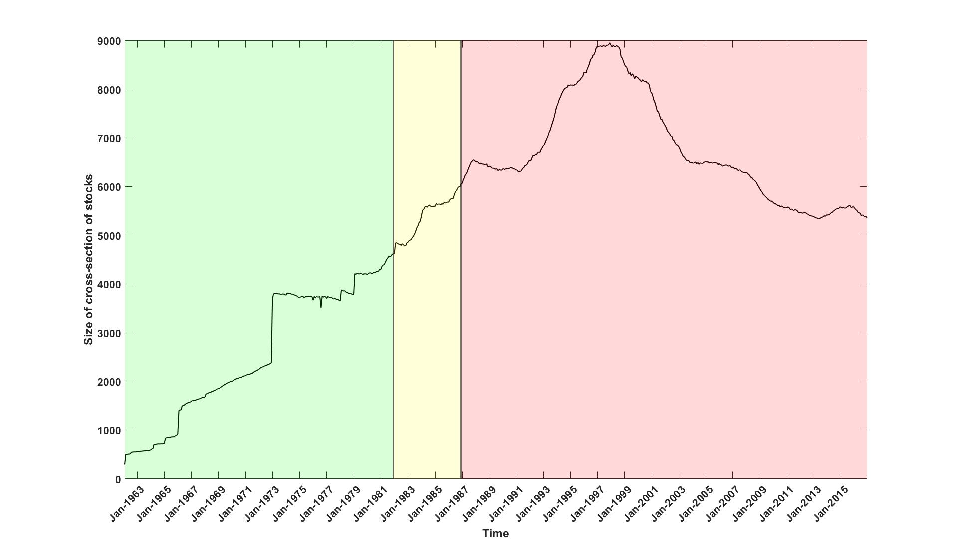
Figure 1: This figure shows the size of the cross-section of stocks in each month of the sample. The full sample is split into training sample (green), Feb 1962 to Dec 1981, validation sample (yellow), Jan 1982 to Dec 1986, and testing sample (red), Jan 1987 to Dec 2016.

3.2 Model selection

We divide the data into three consecutive non-overlapping samples while maintaining the temporal ordering of the data, as shown in Figure 1. The training sample, Feb 1962 to Dec 1981, is used to estimate the hyper-parameters of the Gaussian process. The validation sample, Jan 1982 to Dec 1986, is used for model selection, that is, the kernel function, the mixing weight scheme, the sample splitting scheme (rolling or recursive), and the size of the rolling window if we adopt a rolling scheme. The testing sample, Jan 1987 to Dec 2016, is then used to evaluate the performance of the selected model.

For model selection, we follow a data-driven approach and select the configuration, among all possible combinations, that performs best on the validation sample in terms of prediction accuracy, as measured by $R_{pool}^{2}$. More specifically, we implement our ensemble method for both, rolling and recursive, schemes. In more detail, we apply the rolling scheme for different possible training window lengths $K=2,\ldots,239$. That is, for the MSE weighting scheme (ii) and $K=2$, we use Nov 1981 and Dec 1981 as training and calibration months, respectively, for the first test month, Jan 1982. Likewise, we choose Oct 1986 and Nov 1986, respectively, for the last test month, Dec 1986. Similarly, for the maximal possible $K=239$, we use Feb 1962 to Nov 1981 as training months and Dec 1981 as calibration month for the test month Jan 1982, and shift each by one month for the next test month. This is illustrated in Figure 2. We also apply the recursive scheme, using the full training sample available for each test month. More specifically, we use Feb 1962 to Nov 1981 as training months and Dec 1981 as a calibration month for the test month Jan 1982, while we use Feb 1962 to Oct 1986 as training months and Nov 1986 as calibration month for the last test month Dec 1986. We follow a similar procedure for the equal weighting scheme (i) but without holding out a calibration month.

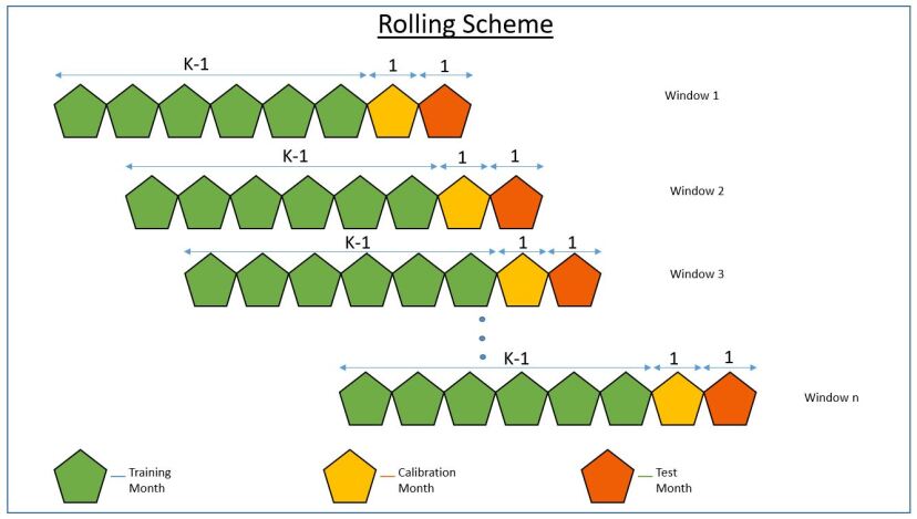
Figure 2: This figure describes the mechanism of the rolling scheme with training window, including a calibration month, of length $K$.

In non-reported preliminary experiments with various kernels, including the squared-exponential, the exponential, and the rational-quadratic ones, the following kernel has outperformed in terms of $R^{2}_{pool}$,

$$k(x,x^{\prime})=\sigma^{2}(1+\alpha\|x\|)(1+\alpha\|x^{\prime}\|)\bigg{(}1+\frac{\|x-x^{\prime}\|}{\beta}\bigg{)}^{-1},$$ (9)

for the hyper-parameters $\sigma,\beta>0$. We note that $\sigma$ is not relevant for the predictive mean in (4) but it is significant in quantifying the Bayesian uncertainty of our predictions, see (5). We therefore report the full empirical analysis only for the kernel (9).

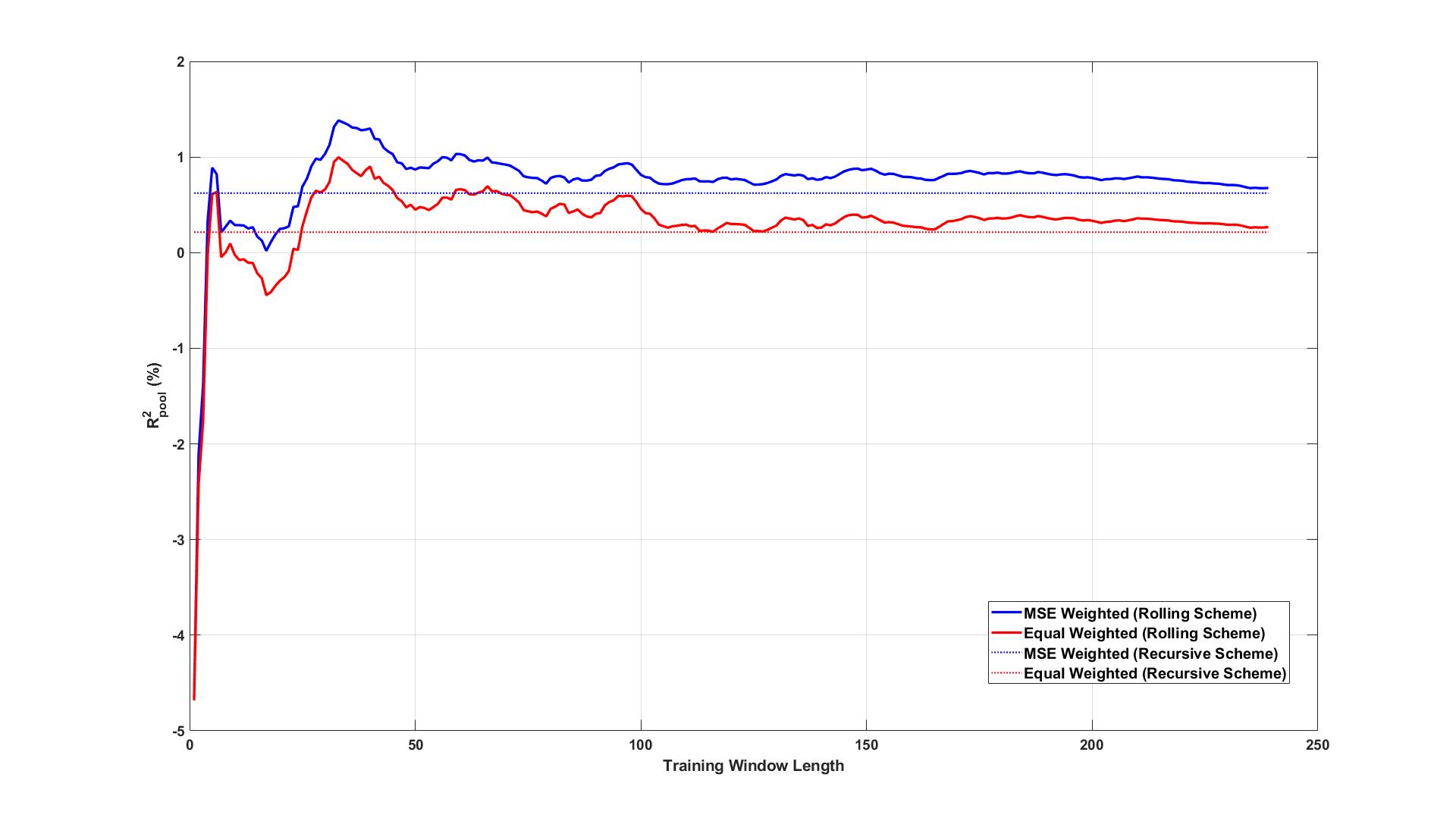
Figure 3: This figure presents $R_{pool}^{2}$ over the validation sample, Jan 1982 to Dec 1986 for equal- and MSE-weighting schemes against the length of the training window. The solid line corresponds to the rolling scheme while the dotted lines represent $R_{pool}^{2}$ for the recursive scheme.

Figure 3 shows $R_{pool}^{2}$ over the validation sample for equal- and MSE-weighting schemes against varying lengths $K$ of the training window. The solid lines correspond to the rolling scheme, while the dotted lines represent $R_{pool}^{2}$ for the recursive scheme, which does not depend on $K$. There are several findings. First, we observe that both sample splitting and mixing weight schemes generate positive $R^{2}_{pool}$ for $K$ large enough ($K>30$). Second, the MSE weighted ensemble yields a larger $R^{2}_{pool}$ than the equal weighted. A possible explanation is the temporal non-stationarity of financial data. There are non-observable changing regimes such that the regime prevailing at any given month $j$ is not explicitly captured by the observable features $\bm{x}_{j-1}$. But it is implicitly captured by the trained Gaussian process $f^{(j)}$ through its fitted hyper-parameters and predictive distribution, given data $\{\bm{x}_{j-1},\,\bm{r}_{j}\}$. The MSE-weighting scheme in turn gives more weight to a training month $j$ the closer its regime is to the current regime prevailing in the calibration month. This results in a more accurate prediction than for equal weighting. Third, it is striking that incorporating the full available training sample, which is the recursive scheme, worsens the predictive performance; as the dotted lines are below the solid lines for both mixing weight schemes. This finding is in line with the bias-variance tradeoff in machine learning, as our ensemble model complexity grows with the size of the training window. Fourth, for the rolling scheme, $R^{2}_{pool}$ is relatively more volatile for small $K$ ($K<50$) and becomes stable and provides considerably more consistent performance for large $K$ ($K>50$). Further, for $K>50$, we observe a peak around $K=100$, which motivates us to choose $K=96$ as the window length for the rolling scheme. To conclude, based on the performance in the validation sample, we select the rolling scheme with training window length $K=96$ and the MSE-weighting scheme for the out-of-sample test.

3.3 Model performance

Having selected the model configuration, we now conduct our empirical analysis over the testing sample. We first train $K-1=95$ individual monthly GPR models, Jan 1979 to Nov 1986, compute MSE weights on the first calibration month, Dec 1986, and use these weights to get the predictive distribution for the returns in the first test month, Jan 1987. We proceed by induction and train one additional GPR model on Dec 1986, combine it with the already trained GPR models on the previous $94$ months, Feb 1979 to Nov 1986, compute MSE weights on the next calibration month, Jan 1987, and predict returns on Feb 1987. We repeat this online learning procedure until the full testing sample is exhausted, consisting of 360 test months until Dec 2016. We evaluate the predictive performance, both statistically and economically, in the following subsections.

3.3.1 Predictive performance across all stocks

Figure 4(a) shows the out-of-sample performance of our model in predicting the returns across time. We plot the time series of monthly $R$-squared, $R_{t}^{2}$ (left scale) and the evolution of $R_{pool}^{2}$ and $R^{2}_{avg}$ over an expanding testing sample (right scale). For example, $R^{2}_{pool}$ ($R^{2}_{avg}$) in Jan 2000 is the pooled $R$-squared (average $R$-squared) evaluated on the testing sample, Jan 1987 to Jan 2000. The positive values of $R^{2}_{pool}$ and $R_{avg}^{2}$ over the expanding testing sample indicates that our model outperforms the zero predictions consistently over time. Moreover, our model achieves $R^{2}_{pool}=1.29\%$ over the full testing sample, which corresponds to Dec 2016 in Figure 4(a). This is substantially greater than the corresponding numbers, 0.4% and 0.58%, for the neural network models in Gu et al. (2020) and Gu et al. (2021), respectively. This shows that our simple approach beats these benchmarks significantly in terms of out-of-sample predictive accuracy measured by $R_{pool}^{2}$. The value $R^{2}_{avg}=0.70\%$ over the full test sample further confirms the superior performance of our model. To assure that small stocks do not drive this unprecedented predictive performance, i.e., that our model is not simply picking up small-scale inefficiencies driven by illiquidity, we measure $R^{2}_{pool}$ on two test subsamples. The first consists of the top-1,000 stocks and the second of the bottom-1,000 stocks by market capitalization each month. The values of $R^{2}_{pool}$ for the two subsamples are 0.76% and 1.19%, respectively. This is indicative that our model is capable of capturing the systematic structure in the large-cap as well as small-cap stocks, although the performance is slightly better for the small-cap stocks. Importantly, our model also dominates the performance on these subsamples, which is 0.7% for large stocks and 0.45% for small stocks, of Gu et al. (2020).

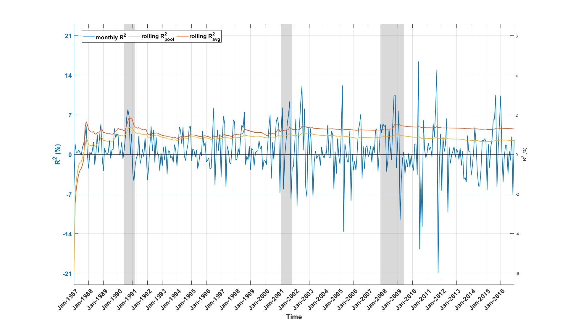
(a) Evolution of $R^{2}_{t}$

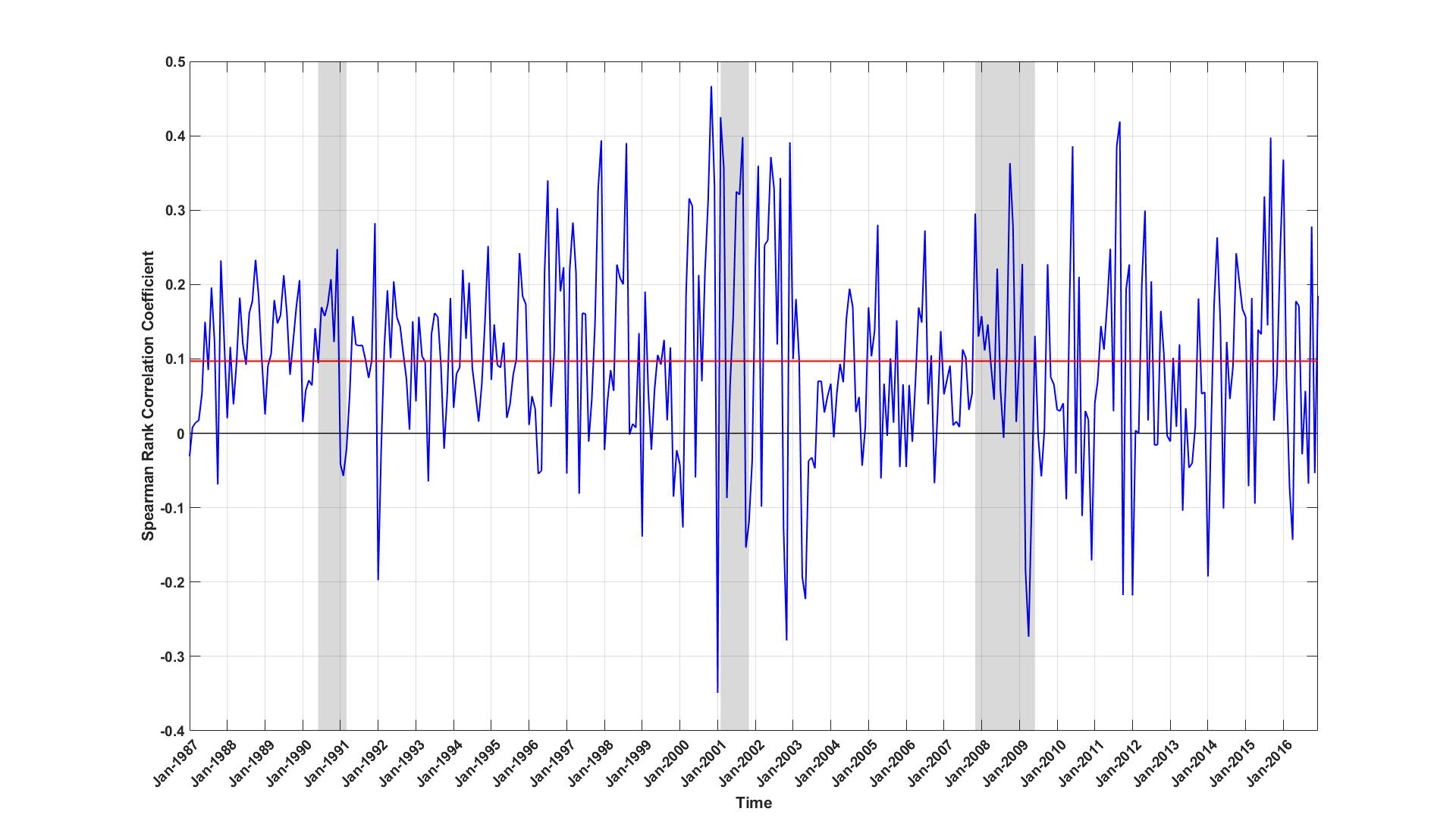
(b) Evolution of Spearman’s rank correlation coefficient

Figure 4: Subfigure 4(a) shows the evolution of $R^{2}_{t}$ over the testing sample (left scale) and evolution of $R^{2}_{pool}$ and $R^{2}_{avg}$ over an expanding testing subsample (right scale). Subfigure 4(b) shows the evolution of Spearman’s rank correlation $\rho_{t}$ between the realized and predicted returns over the testing sample. The flat line gives the information coefficient. The shaded periods indicate NBER recessions.

Figure 4(b) shows the time series of monthly Spearman’s rank correlations $\rho_{t}$ between the predicted and realized returns. The flat line gives the information coefficient, $IC$, our third performance measure. It is evident that there is a substantial variation over time in the ability of our model to differentiate relative performance between stocks, as can be seen by correlation coefficients ranging from -35% to 45%. The information coefficient equals 9.7% and is significantly greater than zero at the 95% confidence level.

Remarkably, we observe that our model performs relatively better during the NBER recession months, as shown by relatively large $R_{t}^{2}$, increases in $R^{2}_{pool}$, and correlation coefficients in the shaded periods of Figures 4(a) and 4(b). We qualify this observation and regress $R_{t}^{2}$ against the excess returns of the S&P 500 over the test sample. Results are shown in Figure 5. The regression coefficient is significantly negative. Indeed, Figure 5 reveals that large positive and negative values of $R_{t}^{2}$ are strongly associated with negative and positive excess returns of the S&P 500, respectively.

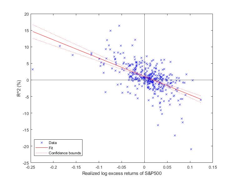
Figure 5: This figure shows the variation of $R_{t}^{2}$ versus S&P 500. The solid red line shows the linear regression line while the dotted red lines show the corresponding confidence bands. The regression coefficient and intercept are -55.36 (4.11) and 1.04 (0.18), respectively, with standard errors in parentheses. Both are significant at the 99.5% confidence level.

3.3.2 Predictive performance across sorted portfolios

So far, our model’s predictive performance assessment has been based on individual stock returns. Next, we analyze the predictive ability of our model at the portfolio level. Why should we assess the portfolio-level predictions when our model is optimized for predicting individual stock returns? We know that one of the main applications of predicting stock returns is to construct portfolios. A model performing better at predicting stock returns need not provide accurate predictions at the portfolio level. Therefore, assessing portfolio forecasts give an additional measure to evaluate the predictive ability of our model.

Given our predictions at the beginning of each test month, we sort stocks into deciles, which we denote by $D1,D2,\ldots,D10$, where $D1$ corresponds to the lowest predicted returns and $D10$ corresponds to the largest predicted returns. Within each decile, we then construct three different portfolios. The first is equal weighted (EW), and the second is value weighted (VW) by market capitalization. These are the standard portfolios in the empirical asset pricing literature. For the third portfolio, we minimize the variance of the Bayesian uncertainty of our predictions by solving the following optimization problem,

$$\min_{{\bm{w}}\in\mathcal{W}}{\bm{w}}^{\top}\hat{{\bm{\Sigma}}}_{t+1}{\bm{w}},$$ (10)

for the predictive covariance matrix $\hat{{\bm{\Sigma}}}_{t+1}$, and where $\mathcal{W}=\{\bm{w};\ \sum_{j\in D}w_{j}=1,\ w_{j}\geq 0,\ j\in D\}$ denotes the feasible set of portfolio weights, for the respective decile $D$. We call it the uncertainty-weighted (UW) portfolio. The goal of studying the predictive performance of the UW portfolio is to examine the role of accuracy estimates in portfolio selection and finally, study its economic contribution when we construct a risk-adjusted portfolio below.

Table 1 shows the out-of-sample predictive performance of sorted portfolios. The top panel reports the $R^{2}_{pool}$ between the predicted excess returns and realized excess returns of the decile portfolios over the test sample for the three different portfolio selection strategies. The bottom panel shows $R^{2}_{pool}$, pooled over all deciles, for each of the three portfolios. It provides a grand portfolio-level assessment of portfolio predictions against the realized portfolio returns. Remarkably, the UW portfolios significantly outperform the EW and VW portfolios in terms of predictive performance across all the deciles, except for $D10$, where EW is slightly better than UW. Further, the UW portfolio yields a positive grand panel $R^{2}_{pool}$ of 1.94% in contrast to EW and VW portfolios that generate a negative grand panel $R^{2}_{pool}$ of -2.18% and -1.76%, respectively. These findings reveal that prediction uncertainties matter.

	Equal-Weighted	Value-Weighted	Uncertainty-Weighted
$D1$	-3.67	-1.56	3.02
$D2$	-5.18	-3.44	-1.99
$D3$	-5.11	-4.44	-1.68
$D4$	-3.70	-3.41	-0.51
$D5$	-2.53	-3.36	0.24
$D6$	-0.53	-2.30	1.78
$D7$	1.38	-0.58	2.73
$D8$	3.95	2.43	5.44
$D9$	6.65	4.95	8.05
$D10$	11.79	7.78	11.71
All	-2.18	-1.76	1.94

Table 1: In this table, we report the out-of-sample predictive performance, measured by $R^{2}_{pool}$ in percentage points, across the sorted portfolios. The first ten rows ($D1$ to $D10$) report $R^{2}_{pool}$ for each decile while the last row (All) reports $R^{2}_{pool}$ calculated over the grand panel of all deciles.

3.3.3 Economic performance of sorted portfolios

Next, we assess whether the improved statistical performance of our prediction-sorted portfolios translates into better economic performance. On top of the EW and VW portfolios discussed in the previous subsection, we introduce two additional portfolios.

First, for the prediction-weighted (PW) portfolio we assign weights, within each decile, to the stocks based on their predicted returns. The goal is to take advantage of the relative strength of the prediction signal in addition to the rankings. Specifically, for each of the top five deciles ($D6$ to $D10$), we subtract the smallest predicted return within the decile to aim at maximal predicted return. Similarly, for each of the bottom five deciles ($D1$ to $D5$), we subtract each predicted return from the largest predicted return within that decile to aim at the minimal predicted return. We then normalized the level-adjusted predicted returns such that they sum up to 1 within each decile. More specifically, for any stock $i$ we define the level-adjusted predicted return

$$\hat{s}_{i,t+1}=\begin{cases}\hat{r}_{i,t+1}-\min_{j\in D_{i}}\hat{r}_{j,t+1},&\text{if $i$ lies in the top 5 deciles, $D6$ to $D10$,}\\ \max_{j\in D_{i}}\hat{r}_{j,t+1}-\hat{r}_{i,t+1},&\text{if $i$ lies in the bottom 5 deciles, $D1$ to $D5$,}\end{cases}$$ (11)

where $\hat{r}_{j,t+1}$ are the predicted returns in decile $D_{i}$ corresponding to stock $i$. These level-adjusted predicted returns are then normalized to obtain portfolio weights,

$$w_{i}=\frac{\hat{s}_{i,t+1}}{\sum_{j\in D_{i}}\hat{s}_{j,t+1}}.$$

Second, the prediction-uncertainty-weighted (PUW) portfolio is motivated by the findings of the previous subsection that the UW portfolio yields a substantially higher $R^{2}_{pool}$ (for each decile) than the EW and VW portfolios. We utilize the predictive covariance matrix and the predicted returns to construct a mean-variance type portfolio for a uncertainty averse investor. We aim at maximizing the portfolio return by investing in stocks with high predicted returns with high accuracy at the same time. More precisely, we combine (10) and (11) by solving the following optimization problem,

$$\max_{{\bm{w}}\in\mathcal{W}}{\bm{w}}^{\top}\hat{{\bm{s}}}_{t+1}-\frac{\gamma}{2}{\bm{w}}^{\top}\hat{{\bm{\Sigma}}}_{t+1}{\bm{w}},$$ (12)

where $\hat{{\bm{s}}}_{t+1}=\{\hat{s}_{j,t+1},\ j\in D\}$ is the vector of level-adjusted predicted returns in the respective decile $D$, and $\gamma$ is the uncertainty-aversion parameter. We set $\gamma=1$ for our performance analysis.

Figure 6 shows the cumulative excess log returns of the VW decile portfolios $D1$ to $D10$. It also shows the cumulative excess log returns of the S&P 500 for comparison. A clear pattern emerges. First, realized returns of the decile portfolios essentially increase monotonically from $D1$ to $D10$. Portfolios based on higher predictions have higher subsequent returns. In particular, the $D1$ portfolio and $D10$ portfolio clearly separate. Second, the $D10$ portfolio outperforms the S&P 500 by a large margin. Similar patterns emerge for the EW, PW, and PUW decile portfolios, as shown in Figures A.3 to A.5 in Appendix C. These findings indicate that our sorted portfolio strategies can consistently dissect the market into high- and low-performing stocks.

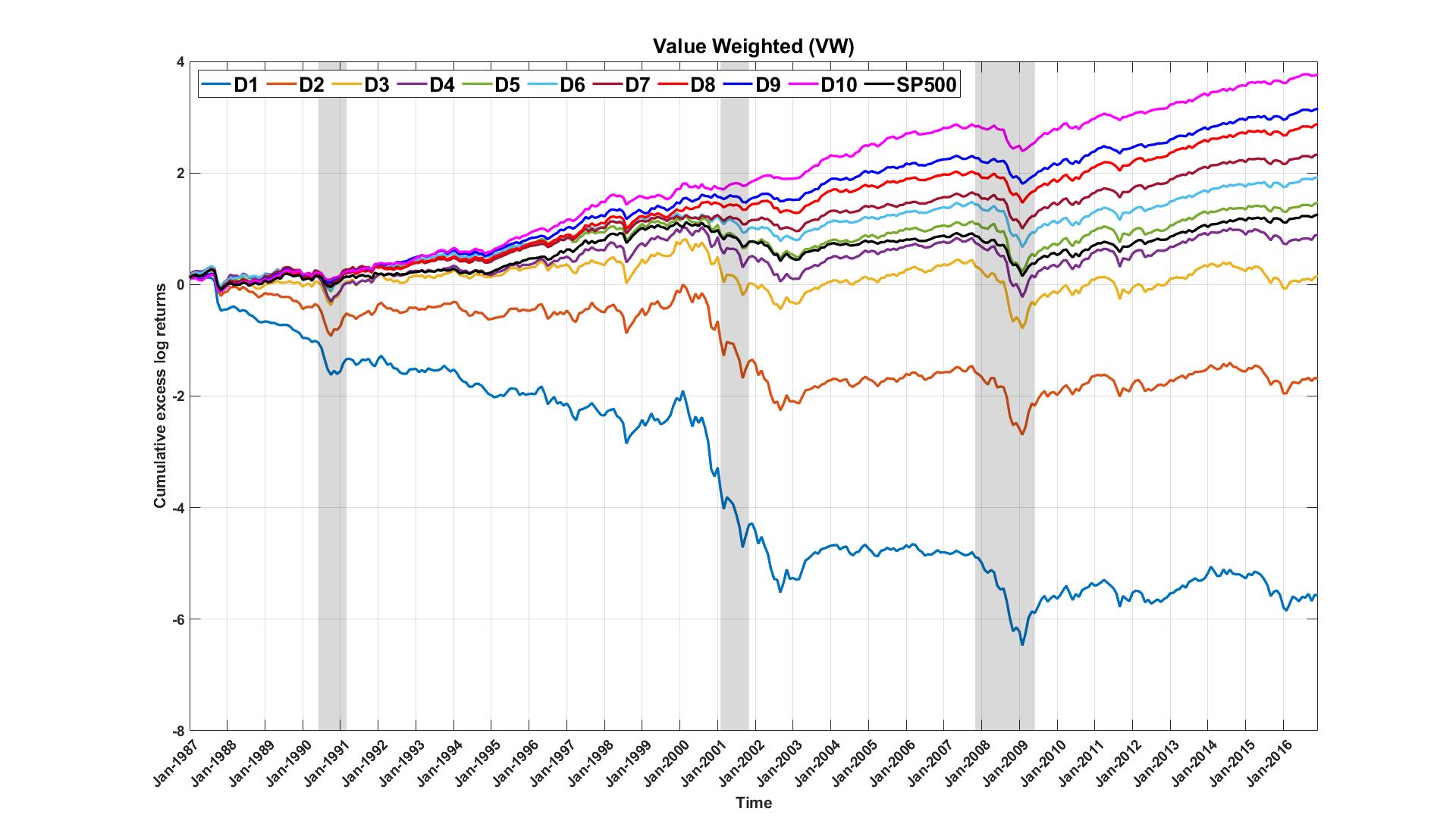
Figure 6: This figure shows the out-of-sample cumulative excess log returns of the VW decile portfolios sorted based on our predicted returns. It also shows the S&P 500. The shaded periods indicate NBER recessions.

In Figure 7, we plot the cumulative excess log returns of the top ($D10$) and bottom ($D1$) decile portfolios for EW, VW, PW, PUW, and the S&P 500. The PUW $D10$ portfolio yields a cumulative excess log return of 7.28. The PUW $D1$ portfolio, on other side, yields a cumulative excess log return of -16.7. The large difference in cumulative returns from these two portfolios shows that our model is not only good at dissecting the stock market into deciles but also at predicting the relative return levels within a decile. Remarkably, the uncertainty averse PUW portfolio dominates the performance of the EW, VW, and PW portfolios by a large margin in both directions, top and bottom. These findings show that exploiting the Bayesian nature of GPR by incorporating uncertainty in the predictions can significantly improve portfolio performance. Interestingly, the bottom decile portfolio performance is essentially flat in the post-2000 sample, except for PUW. This observation has also been reported in Gu et al. (2020).

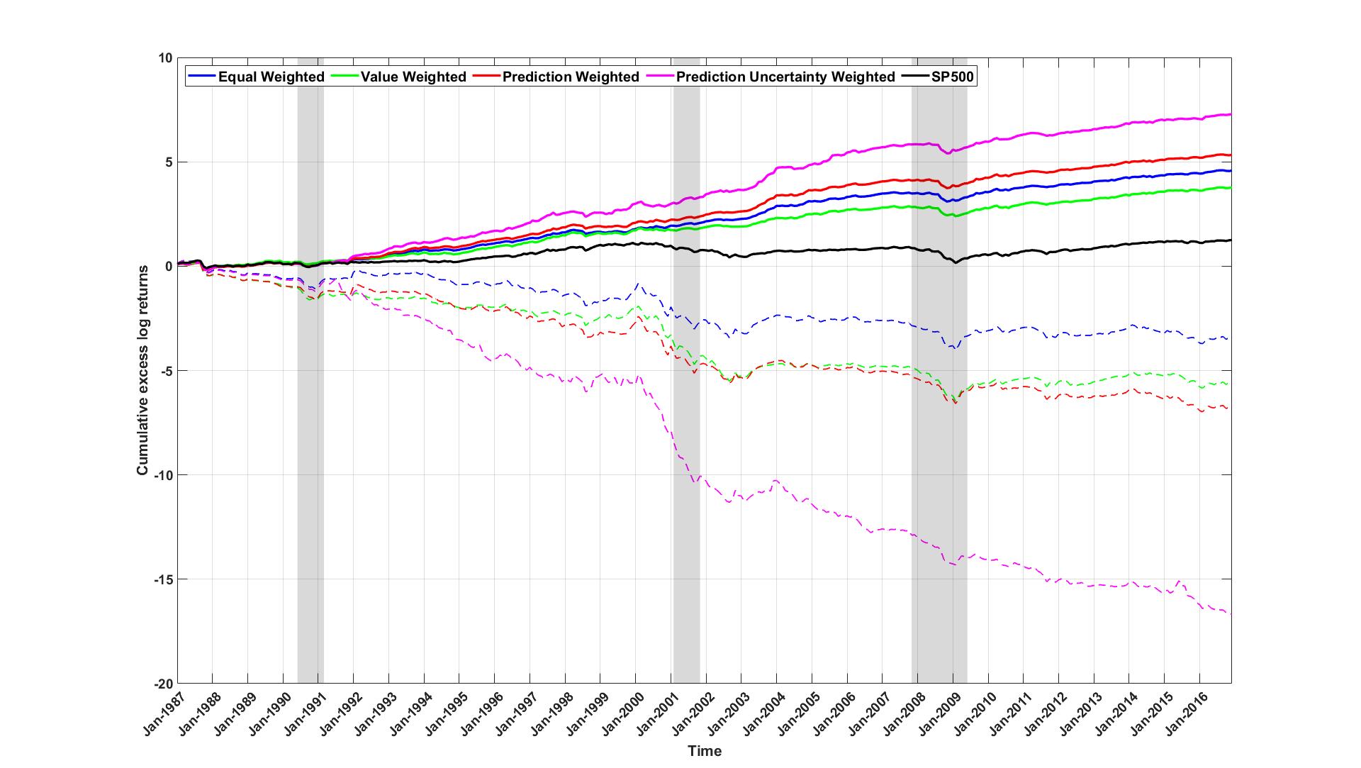
Figure 7: This figure shows the out-of-sample cumulative excess log returns of the $D10$ (solid lines) and $D1$ (dashed lined) portfolios for EW, VW, PW and PUW, sorted based on our predicted returns. It also shows the S&P 500. The shaded periods indicate NBER recessions.

We also construct a zero-net-investment portfolio that is long $D10$ and short $D1$ for EW, VW, PW, and PUW. Figure 8 shows their cumulative excess log returns. The qualitative conclusions are identical to what we observed in Figure 7.

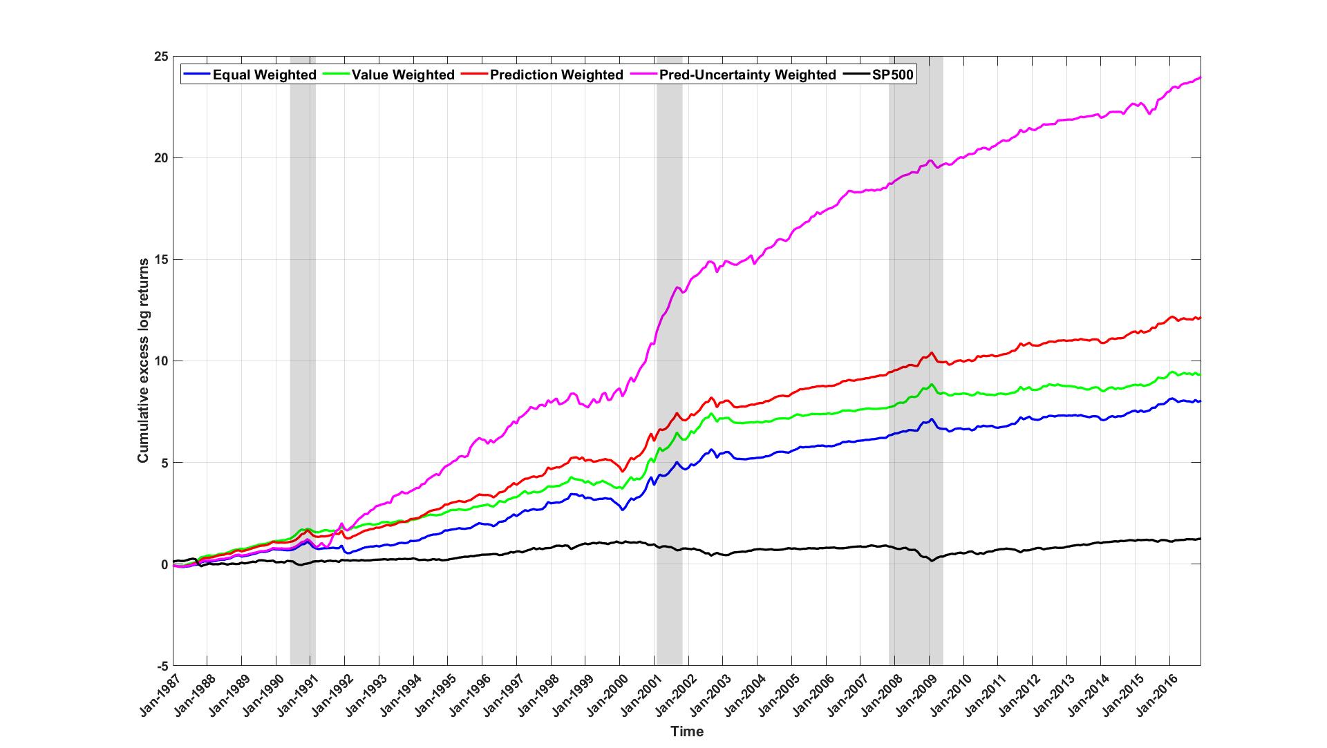
Figure 8: This figure shows the cumulative excess log returns of the long-short portfolios for EW, VW, PW and PUW, obtained by taking a long position in the $D10$ and short position in $D1$ portfolios. It also shows the S&P 500. The shaded periods indicate NBER recessions.

We evaluate the performance of our four $D10$ and $D1$ portfolios, and the S&P 500 as benchmark, in terms of their annualized mean return, standard deviation, and Sharpe ratio. These metrics are calculated based on simple excess returns, and are collected in Table 2. The highest Sharpe ratio of 1.447 is attained by the PUW $D10$ portfolio, which significantly outperforms the S&P 500 with a Sharpe ratio of 0.36. The PW $D10$ portfolio also performs well, with a Sharpe ratio of 1.392, and dominates the EW and VW $D10$ portfolios. This reconfirms that our model is good at predicting the ranks of stock returns as well as their levels relative to other stocks within the same decile. The same holds, in the negative direction, for the $D1$ portfolios. The long-short PUW portfolio generates a huge annualized mean return of 68.5%, but it comes at the expense of a high standard-deviation of 47.6%. Nonetheless, it outperforms the S&P 500 by a significant margin and could potentially be a suitable choice for a risk-seeking investor. Our findings suggests that taking into account the levels of return predictions and the uncertainty estimates of the predictions significantly improves the performance of the PW and PUW portfolios in comparison to EW and VW. The latter are the portfolio strategies that are typically studied in the literature.

Our performance compares favorably to Gu et al. (2020), who report Sharpe ratios of 1.0 and 0.8 for EW and VW $D10$ portfolios, -0.4 and -0.19 for the EW and VW $D1$ portfolios, and 2.36 (2.63) and 1.2 (1.53) for EW and VW long-short portfolios (in Gu et al. (2021)).

	Top Decile $D10$
	EW	VW	PW	PUW	SP500
Mean	0.162	0.135	0.189	0.262	0.054
SD	0.127	0.130	0.136	0.181	0.150
Sharpe	1.274	1.042	1.392	1.447	0.360
	Bottom Decile $D1$
	EW	VW	PW	PUW	SP500
Mean	-0.053	-0.122	-0.155	-0.423	0.054
SD	0.359	0.347	0.380	0.498	0.150
Sharpe	-0.147	-0.352	-0.408	-0.849	0.360
	Long–Short
	EW	VW	PW	PUW	SP500
Mean	0.215	0.257	0.344	0.685	0.054
SD	0.298	0.285	0.323	0.476	0.150
Sharpe	0.721	0.902	1.063	1.441	0.360

Table 2: In this table, we report the mean excess return, standard deviation (SD), and Sharpe ratio of $D10$, $D1$ and long-short portfolios corresponding to EW, VW, PW and PUW. We calculate these measures using realized simple excess returns of the portfolios over the testing sample. We also report these measures for the S&P 500 for comparison. All measures are annualized.

We end by a disclaimer noting that the performance of the above portfolios does not take into account any transaction costs, which, when considered, could offset the gains. Importantly, our dataset contains highly illiquid stocks with extremely small market capitalization. These stocks are thus unlikely to be accessible to investors and may incur significant transaction costs due to high bid-ask spreads and low liquidity. Hence, an investor could not potentially exploit the higher gains by shorting the $D1$ portfolio. But this applies to the benchmarks as well. We qualify the relation between market capitalization and predicted returns in Appendix B.

4 Conclusion

The out-of-sample prediction of conditional expected stock returns remains a central challenge in empirical asset pricing. In this paper, we introduce a novel ensemble GPR method to predict conditional expected returns. While we do not claim that our simple method is the best approach for all situations, we find that it outperforms the benchmarks by significant margins in terms of $R$-squared. Exploiting the Bayesian nature of GPR, we also model and quantify the prediction uncertainty, which leads to significant economic gains in terms of the performance of uncertainty-weighted prediction-sorted portfolios. Our ensemble approach reduces the computational complexity inherent in GPR and addresses the non-stationarity and heteroscedasticity in financial data. As such, it lends itself to a variety of online learning tasks to be explored in future research.

Appendix A Gaussian Process Regression

In this appendix we give an introduction to Gaussian process regression. For more background and theory we refer the reader to Williams and Rasmussen [2006].

A.1 Gaussian Processes

A Gaussian process is a collection of random variables, any finite number of which have a joint Gaussian distribution. More specifically, let $\mathcal{X}$ be a non-empty set. A random function $f:\mathcal{X}\rightarrow{\mathbb{R}}$ is a Gaussian process (GP) with mean function $m(\cdot)$ and covariance function, or, kernel $k(\cdot,\cdot)$, if for any finite set $\bm{x}=(x_{1},x_{2},\ldots,x_{n})\subset\mathcal{X}$ the random vector

$$f(\bm{x})=(f(x_{1}),f(x_{2}),\ldots,f(x_{n}))^{\top}$$

follows multivariate normal distribution $\mathcal{N}(m(\bm{x}),k(\bm{x},\bm{x}^{\top}))$ with mean vector

$$m(\bm{x})=(m(x_{1}),m(x_{2}),\ldots,m(x_{n}))^{\top}$$

and covariance matrix

$$k(\bm{x},\bm{x}^{\top})=(k(x_{i},x_{j}))^{n}_{i,j=1}.$$

A.2 Training GPR

To fit the hyper-parameters by maximum likelihood, we compute the partial derivatives of the marginal likelihood function (6) w.r.t. the hyper-parameters,

$$\frac{\partial}{\partial\theta_{j}}\log p(\bm{y}\mid{\bm{X}},\theta) =-\frac{{\bm{y}}^{\top}K_{y}^{-1}\frac{\partial K_{y}}{\partial\theta_{j}}K_{y}^{-1}{\bm{y}}}{2}-\frac{1}{2}tr\bigg{(}K_{y}^{-1}\frac{\partial K_{y}}{\partial\theta_{j}}\bigg{)}$$ (13)

$$=\frac{1}{2}tr\bigg{(}(K_{y}^{-1}{\bm{y}}{\bm{y}}^{\top}K_{y}^{-1}-K_{y}^{-1})\frac{\partial K_{y}}{\partial\theta_{j}}\bigg{)}$$

where we write $K_{y}={\bm{K}}+\sigma_{\epsilon}^{2}I$. We then find the optimal hyper-parameters $\hat{\theta}$ by any gradient based optimizer and gradient given in (13).

Appendix B Relation between market capitalization and predicted returns

We qualify the discussion on liquidity and show that the market capitalization of a stock is positively associated with its predicted return. Figure A.1 shows the time series of monthly Spearman’s rank correlation $\rho_{t}$ between the predicted returns and market capitalization of stocks. The flat red line shows the average Spearman’s rank correlation and is equal to 0.3. Figure A.2 shows the time-averaged cross-sectional copula of the market capitalization and predicted return of the stocks, at the resolution of deciles. The mass of the copula is concentrated on the diagonal cells, which affirms our hypothesis. We conclude that stocks in the top decile $D10$ in terms of predicted returns are more likely to have a large market capitalization, and thus be highly liquid. The converse holds for $D1$. Hence our economic performance metrics are of practical relevance mainly for the liquid $D10$ portfolios.

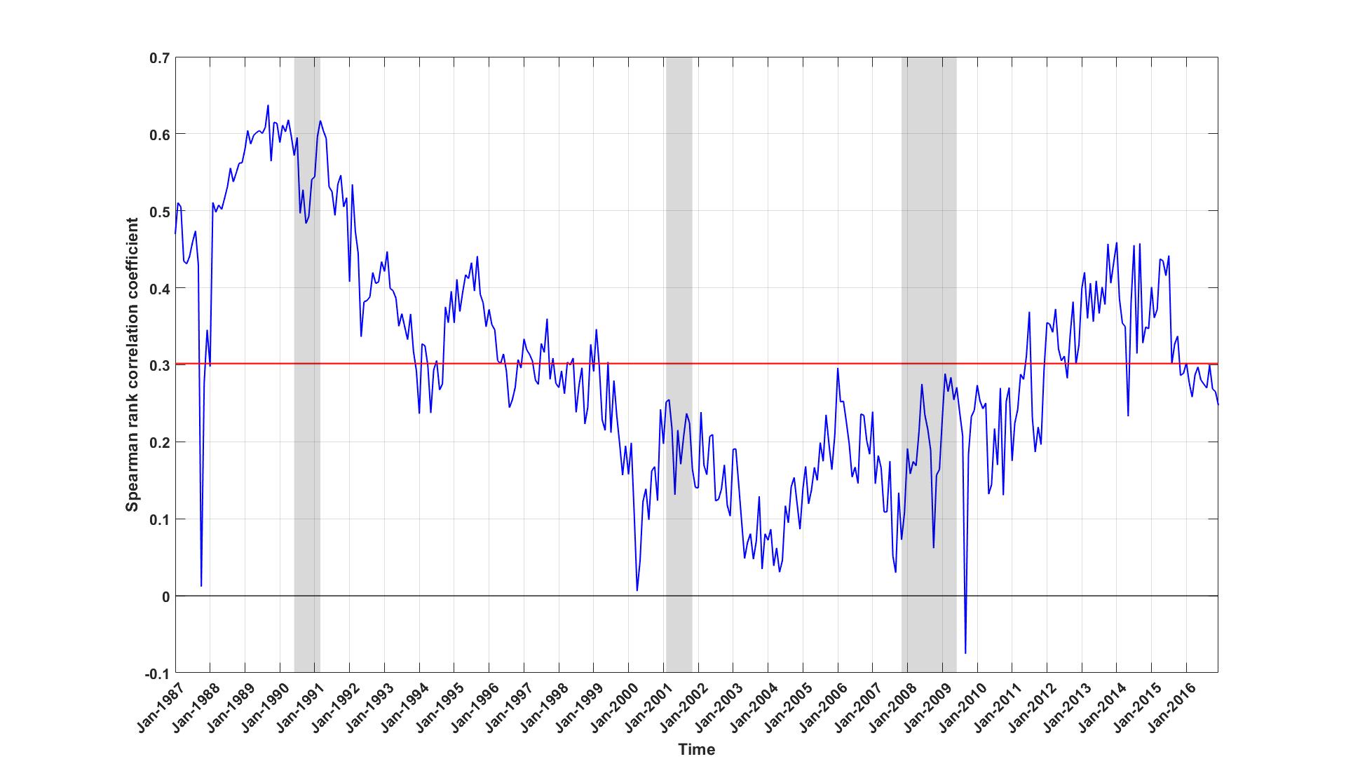
Figure A.1: This figure shows the evolution of Spearman’s rank correlation coefficient between predicted returns and market capitalization of the stocks. Red line shows the average Spearman’s rank correlation. The shaded periods indicate NBER recessions.

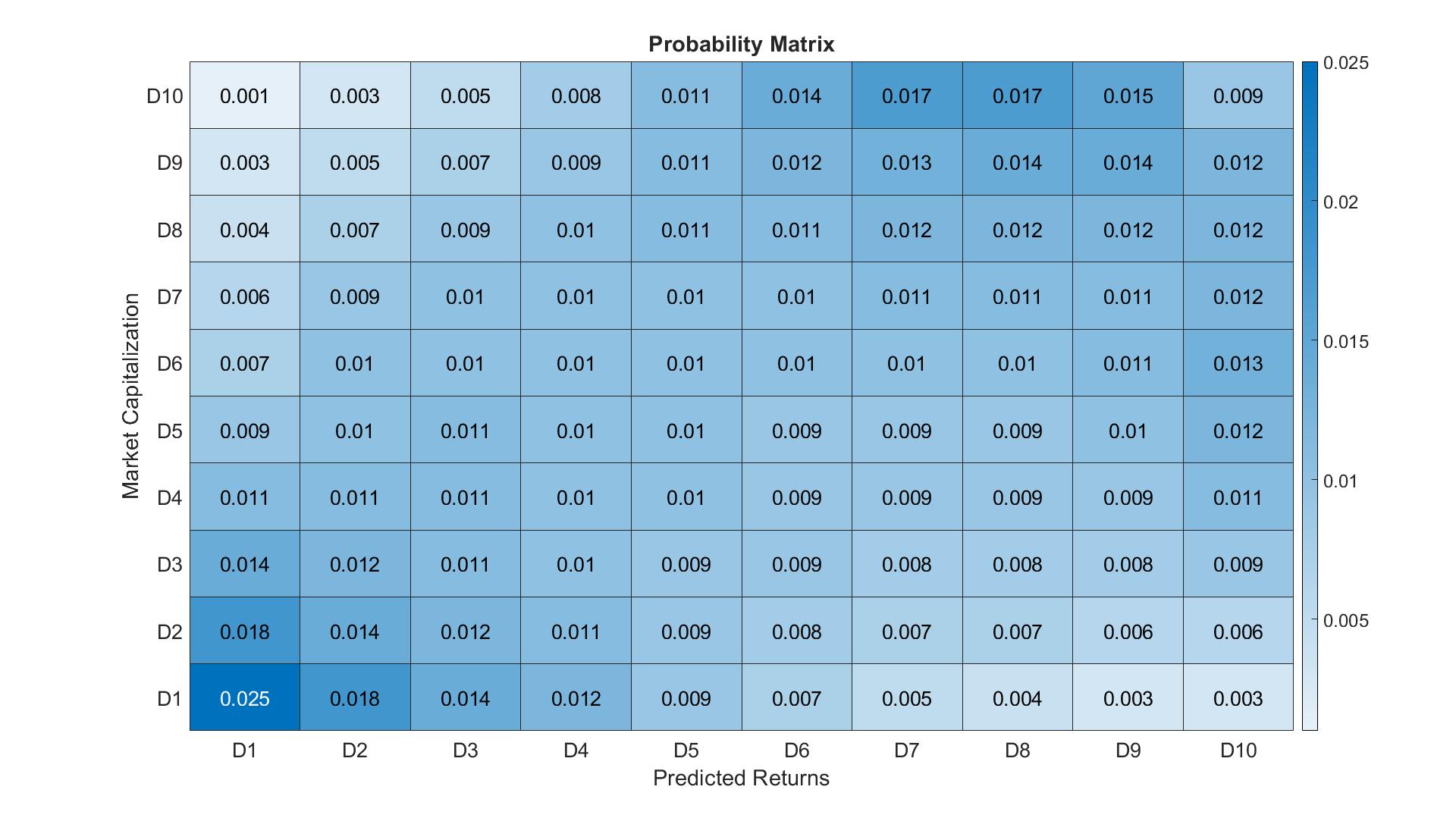
Figure A.2: This figure shows the time-averaged cross-sectional copula of the market capitalization and predicted return of the stocks, at the resolution of deciles. More specifically, the $ij$th entry in this matrix gives probabilities (averaged over test period) that a predicted return in $j$th decile (based on predicted returns) falls in $i$th decile (based on market capitalization).

Appendix C Other plots

This appendix contains additional plots that are mentioned in the main text.

Figure A.3: This figure shows the cumulative excess log returns of equal weighted (EW) decile portfolios sorted based on our predicted returns. It also shows the S&P 500. The shaded periods indicate NBER recessions.

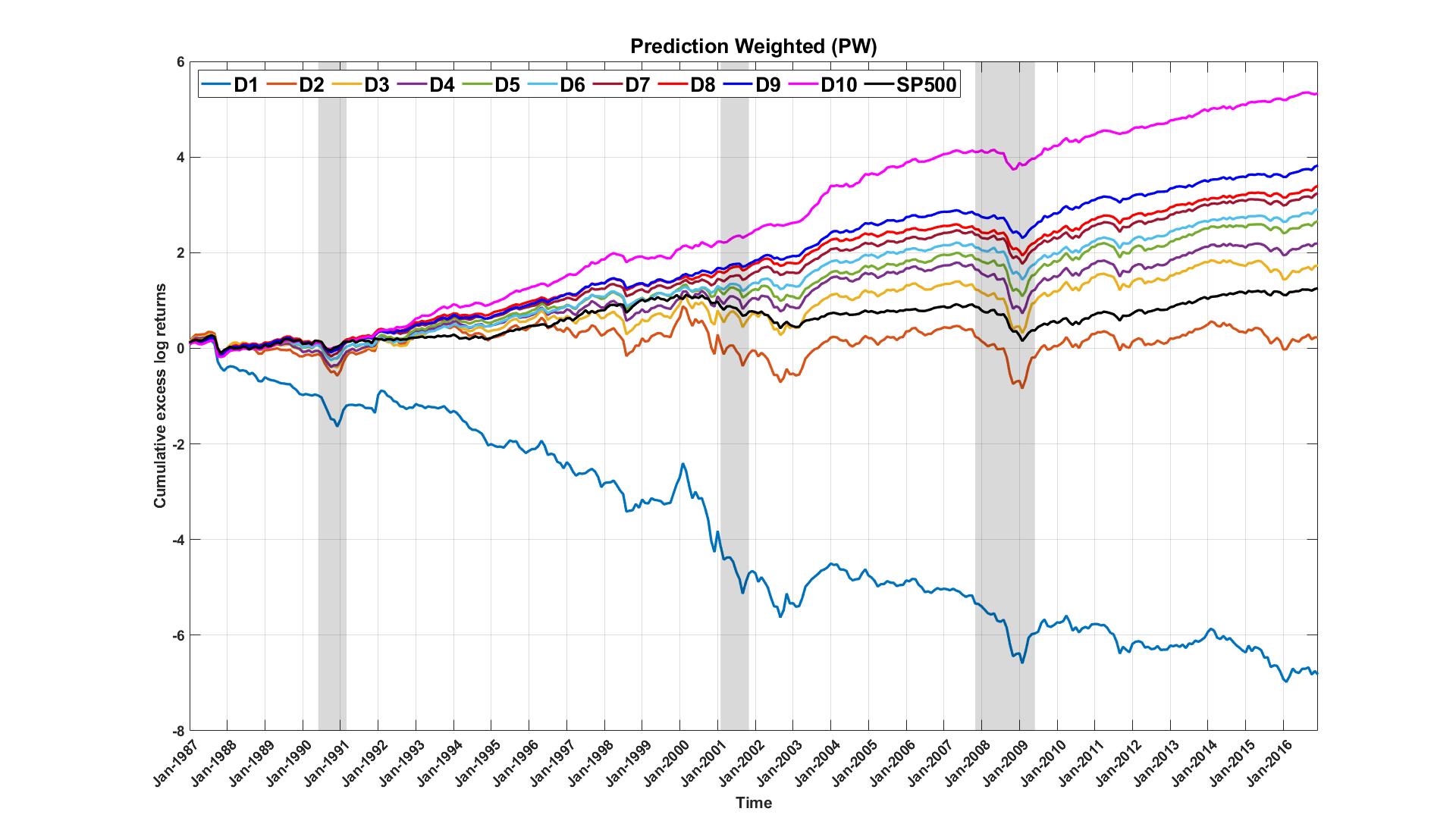
Figure A.4: This figure shows the cumulative excess log returns of prediction weighted (PW) decile portfolios sorted based on our predicted returns. It also shows the S&P 500. The shaded periods indicate NBER recessions.

Figure A.5: This figure shows the cumulative excess log returns of prediction-uncertainty-weighted (PUW) decile portfolios sorted based on our predicted returns. It also shows the S&P 500. The shaded periods indicate NBER recessions.

References

- Ambachtsheer [1974] K. P. Ambachtsheer. Profit potential in an “almost efficient” market. The Journal of Portfolio Management, 1(1):84–87, 1974.
- Asness et al. [2019] C. S. Asness, A. Frazzini, and L. H. Pedersen. Quality minus junk. Review of Accounting Studies, 24(1):34–112, 2019.
- Avramov et al. [2020] D. Avramov, S. Cheng, and L. Metzker. Machine learning versus economic restrictions: Evidence from stock return predictability. available at ssrn 3450322, 2020.
- Bianchi et al. [2021] D. Bianchi, M. Büchner, and A. Tamoni. Bond risk premiums with machine learning. The Review of Financial Studies, 34(2):1046–1089, 2021.
- Cao and Fleet [2014] Y. Cao and D. J. Fleet. Generalized product of experts for automatic and principled fusion of Gaussian process predictions. arXiv preprint arXiv:1410.7827, 2014.
- Casella et al. [2010] G. Casella, M. Ghosh, J. Gill, and M. Kyung. Penalized regression, standard errors, and Bayesian lassos. Bayesian Analysis, 5(2):369–411, 2010.
- Chen et al. [2022] L. Chen, M. Pelger, and J. Zhu. Deep learning in asset pricing. Management Science, Forthcoming, 2022.
- Cousin et al. [2016] A. Cousin, H. Maatouk, and D. Rullière. Kriging of financial term-structures. European Journal of Operational Research, 255(2):631–648, 2016.
- De Spiegeleer et al. [2018] J. De Spiegeleer, D. B. Madan, S. Reyners, and W. Schoutens. Machine learning for quantitative finance: fast derivative pricing, hedging and fitting. Quantitative Finance, 18(10):1635–1643, 2018.
- Deisenroth and Ng [2015] M. Deisenroth and J. W. Ng. Distributed Gaussian processes. In International Conference on Machine Learning, pages 1481–1490. PMLR, 2015.
- Drobetz and Otto [2021] W. Drobetz and T. Otto. Empirical asset pricing via machine learning: evidence from the European stock market. Journal of Asset Management, 22(7):507–538, 2021.
- Fama and French [2008] E. F. Fama and K. R. French. Dissecting anomalies. The Journal of Finance, 63(4):1653–1678, 2008.
- Farrell et al. [2021] M. H. Farrell, T. Liang, and S. Misra. Deep neural networks for estimation and inference. Econometrica, 89(1):181–213, 2021.
- Filipović and Pasricha [2022] D. Filipović and P. Pasricha. Copula process models for financial risk management. Swiss Finance Institute Working Paper, 2022.
- Filipović et al. [2022a] D. Filipović, M. Pelger, and Y. Ye. Shrinking the term structure. Swiss Finance Institute Research Paper, (22-61), 2022a.
- Filipović et al. [2022b] D. Filipović, M. Pelger, and Y. Ye. Stripping the discount curve–a robust machine learning approach. Swiss Finance Institute Research Paper, (22-24), 2022b.
- Giordano et al. [2002] F. Giordano, M. L. Rocca, and C. Perna. Standard error estimation in neural network regression models: the AR-Sieve bootstrap approach. In Neural Nets WIRN Vietri-01, pages 201–206. Springer, 2002.
- Gu et al. [2020] S. Gu, B. Kelly, and D. Xiu. Empirical Asset Pricing via Machine Learning. The Review of Financial Studies, 33(5):2223–2273, 2020.
- Gu et al. [2021] S. Gu, B. Kelly, and D. Xiu. Autoencoder asset pricing models. Journal of Econometrics, 222(1):429–450, 2021.
- Guhaniyogi et al. [2017] R. Guhaniyogi, C. Li, T. D. Savitsky, and S. Srivastava. A divide-and-conquer Bayesian approach to large-scale kriging. arXiv preprint arXiv:1712.09767, 2017.
- Han et al. [2016] J. Han, X.-P. Zhang, and F. Wang. Gaussian process regression stochastic volatility model for financial time series. IEEE Journal of Selected Topics in Signal Processing, 10(6):1015–1028, 2016.
- Kaniel et al. [2022] R. Kaniel, Z. Lin, M. Pelger, and S. Van Nieuwerburgh. Machine-learning the skill of mutual fund managers. Technical report, National Bureau of Economic Research, 2022.
- Kelly et al. [2019] B. T. Kelly, S. Pruitt, and Y. Su. Characteristics are covariances: A unified model of risk and return. Journal of Financial Economics, 134(3):501–524, 2019.
- Koijen et al. [2018] R. S. Koijen, T. J. Moskowitz, L. H. Pedersen, and E. B. Vrugt. Carry. Journal of Financial Economics, 127(2):197–225, 2018.
- Ng and Deisenroth [2014] J. W. Ng and M. P. Deisenroth. Hierarchical mixture-of-experts model for large-scale Gaussian process regression. arXiv preprint arXiv:1412.3078, 2014.
- Tresp [2000] V. Tresp. A Bayesian committee machine. Neural Computation, 12(11):2719–2741, 2000.
- Wager et al. [2014] S. Wager, T. Hastie, and B. Efron. Confidence intervals for random forests: The jackknife and the infinitesimal jackknife. The Journal of Machine Learning Research, 15(1):1625–1651, 2014.
- Welch and Goyal [2008] I. Welch and A. Goyal. A comprehensive look at the empirical performance of equity premium prediction. The Review of Financial Studies, 21(4):1455–1508, 2008.
- Williams and Rasmussen [2006] C. K. Williams and C. E. Rasmussen. Gaussian processes for machine learning. MIT press Cambridge, MA, 2006.