Computer assisted proof of homoclinic chaos
in the spatial equilateral restricted four body problem

Abstract

We develop computer assisted arguments for proving the existence of transverse homoclinic connecting orbits, and apply these arguments for a number of non-perturbative parameter and energy values in the spatial equilateral circular restricted four body problem. The idea is to formulate the desired connecting orbits as solutions of certain two point boundary value problems for orbit segments which originate and terminate on the local stable/unstable manifolds attached to a periodic orbit. These boundary value problems are studied via a Newton-Kantorovich argument in an appropriate Cartesian product of Banach algebras of rapidly decaying sequences of Chebyshev coefficients. Perhaps the most delicate part of the problem is controlling the boundary conditions, which must lie on the local stable/unstable manifolds of the periodic orbit. For this portion of the problem we use a parameterization method to develop Fourier-Taylor approximations equipped with a-posteriori error bounds. This requires validated computation of a finite number of Fourier-Taylor coefficients via Newton-Kantorovich arguments in appropriate Cartesian product of rapidly decaying sequences of Fourier coefficients, followed by a fixed point argument to bound the tail terms of the Taylor expansion. Transversality follows as a consequence of the Newton-Kantorovich argument.

1 Introduction

The goal of the present work is to prove the existence of chaotic dynamics in a particular restricted gravitational four body problem. The restriction is that the orbits of three of the bodies, called the primaries, are constrained to the equilateral triangle configuration of Lagrange. That is, at each instant the primaries are located at the vertices of an equilateral triangle, rigidly rotating with constant angular velocity about the center of mass. Considered singly, the orbit of each primary is a Keplerian circle about their center of mass. The three circles need not be the same: they coincide if and only if the masses of the three bodies have equal mass.

One now introduces a fourth, massless particle moving under the gravitational influence of the three massive primaries. Imagine a man-made space craft/satellite or small natural astroid/comet. Changing to a co-rotating coordinate frame fixes the locations of the primary bodies, and the equations of motion for the massless particle are now autonomous, albeit in a non-inertial frame. The problem is referred to as the equilateral restricted four body problem, or simply the circular restricted four body problem (CRFBP), and it was derived and first studied by Pedersen [46, 47] in the mid 1940’s and 50’s. Interest in the problem was revived in the late 1970’s, after the study of Simó [52]. The equations of motion are given explicitly in Section 1.1.

The plane of the triangle is an invariant subsystem, and chaotic motions in the planar problem have been established in a number of different contexts. For example the authors of [21, 51, 50] prove the existence of planar chaotic motions by taking the mass of the second and third primary equal and very small. More precisely, they obtain the existence of planar chaos in CRFBP using Melnikov analysis and perturbing out of the planar Kepler problem. Chaos via the mechanism of Devaney (see [22]) is studied in [11], again in the case that the second and third masses are small and equal. For non-equal, and non-perturbative masses $m_{1}=0.5,m_{2}=0.3,m_{3}=0.2$ (the same non-symmetric mass values studied in [52]), the authors of [31] show the existence of planar chaotic motions by directly verifying the hypotheses of Devaney’s theorem. The proof is computer assisted.

In the present work we consider the spatial CRFBP, and prove the existence of out of plane chaotic dynamics. The idea of our proof is to directly verify the hypotheses of Smale’s homoclinic tangle theorem [53], using constructive computer assisted methods. Recall that – in brief – the Smale theorem says the existence of a transverse homoclinic to a periodic solution of an ODE implies chaos. In an earlier work [43], the present authors provide numerical evidence suggesting the existence spatial chaos in the CRFBP. The idea was to study the vertical Lyapunov families of periodic orbits attached to the the saddle-focus libration points of the CRFBP. These saddle-focus libration points were shown to admit planar homoclinic orbits in [31], and in [43] we used these planar homoclinics to locate approximate homoclinic connections for vertical Lyapunov family. These approximations were projected onto parameterizations of the stable/unstable manifolds of the periodic orbits, and refined via a differential corrections/Newton scheme.

The present work begins where [43] left off. That is, we develop an a-posteriori argument which allows us to pass from the numerical evidence in [43] to a mathematically rigorous (computer assisted) proof of the existence of spatial Smale horseshoes in the CRFBP. We remark that computer assisted proofs of chaos in the planar restricted three body problem (as opposed to the four body case considered here) were established in [3] for the case of equal masses, and in [58, 59, 15] for the Sun-Jupiter mass values. These works exploit Poincare sections (restricted to an energy manifold), a strategy which reduces the problem to a question about intersections of one dimensional arcs in the plane. Exploiting this reduction in the spatial case leads to questions about intersections of two dimensional manifolds for four dimensional Poincare maps, and visualizing the problem is much more difficult.

While the geometric methods used by the authors just cited can certainly be extended to higher (even infinite dimensions - see for example [60]), we choose an alternative approach, which is to develop a-posteriori analysis for the BVP set up utilized in [43], working directly with the periodic orbits, their attached local invariant manifolds, and connecting orbit segments between them in the six dimensional phase space of the ODE. Actually –since our approach requires extensive manipulation of Taylor, Fourier, Chebyshev, and Fourier-Taylor series – we find it convenient to append three additional differential equations, effectively embedding the CRFBP into a nine dimensional polynomial system of ODEs. (This polynomial embedding is reviewed in 1.1).

In this sense, the present work builds on the earlier work of [36, 13] on computer assisted Fourier analysis of periodic orbits, the work of [20] on validated Fourier-Taylor computation of local stable/unstable manifolds attached to periodic orbits, and the works of [38, 54, 56] on computer assisted proofs for two point BVPs projected into Chebyshev space. One important technical point is that, since we work with higher dimensional manifolds and in a higher dimensional phase than in these prior works, we find it convenient to formulate the a-posteriori error analysis using a “matrix free” approach, similar to that developed for Taylor series in [4, 40]. That is, we do not employ a Newton-Like operator in the error analysis of the stable/unstable manifolds of the periodic orbits, and hence avoid working with large interval matrices. Rather, we formulate a fixed point problem on an appropriate space of “Fourier-Taylor tails” which – for a given choice of the truncation order – contracts for appropriate choices of the scalings of the stable/unstable bundle parameterizations. It is also important to note that one pair of parameterized stable/unstable manifolds (with validated error bounds) can be used in many different computer assisted proofs of distinct connecting orbits. This provides one justification of the computational effort which goes into studying them.

The remainder of the paper is organized as follows. In the next subsection we review the Equations of motion for the CRFBP 1.1. Section 2 reviews background material on the parameterization method, Banach algebras of rapidly decaying coefficients, and a-posteriori analysis needed in the remainder of the paper. In Section 3 we discuss the computer assisted techniques for proving the existence of the periodic orbits, performing validated computations of their stable/unstable normal bundles, solving the homological equations describing the jets of the stable/unstable manifolds, and establishing the existence of connecting orbits via the solution of two point boundary value problems. Mathematically rigorous bounds on the tail of the Fourier-Taylor expansion of the stable/unstable manifold are developed in 4. In Section 5 we discuss our main results, and several appendices describe some more technical/tedious bounds. The computer codes which execute the computer assisted portions of our arguments are implemented in MatLab using the IntLab library for managing round off errors [49], and are freely available on the homepage of the second author:

https://cosweb1.fau.edu/~jmirelesjames/spatialCRFBP_CAP_chaos.html

1.1 The (Spatial) Equilateral Restricted Four Body Problem

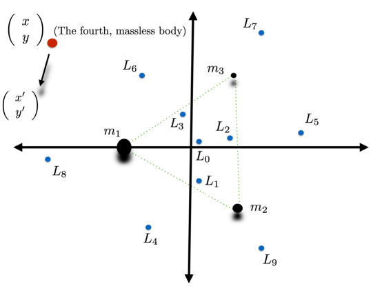
Figure 1: Configuration space for the CRFBP: The three primary bodies with masses $m_{1},m_{2},$ and $m_{3}$ are arranged in the equilateral triangle configuration of Lagrange – a relative equilibrium solution of the three body problem. Transforming to a co-rotating frame one considers the motion of a fourth massless body. The equations of motion have $8$, $9$, or $10$ equilibrium solutions denoted by $\mathcal{L}_{j}$ for $0\leq j\leq 9$. The number of libration points, and their stability, varies depending on $m_{1}$, $m_{2}$, and $m_{3}$. In this work we study the points $\mathcal{L}_{0,4,5,6}$ which have saddle focus stability when $m_{1}\approx m_{2}\approx m_{3}$.

Let the three primary bodies have masses $m_{1}$, $m_{2}$ and $m_{3}$, normalized so that $0<m_{3}\leq m_{2}\leq m_{1}$, and

$$m_{1}+m_{2}+m_{3}=1.$$

We sometimes refer to the primary bodies simply as $m_{1},m_{2},$ and $m_{3}$. Further normalizations allow taking the center of mass at the origin, the position of $m_{1}$ on the negative $x$-axis, and $m_{3}$ is in the first quadrant.

Under these constraints, the locations of the primaries are functions of the masses $m_{1},m_{2},m_{3}$ only. That is, letting

$$p_{j}=(x_{j},y_{j},z_{j}),\quad\quad\quad\mbox{for }j=1,2,3,$$

denote the positions of the primary bodies in the rotating coordinate system, and defining

$$K=m_{2}(m_{3}-m_{2})+m_{1}(m_{2}+2m_{3}),$$

it can be shown that

$$x_{1} = \frac{-|K|\sqrt{m_{2}^{2}+m_{2}m_{3}+m_{3}^{2}}}{K}$$

$$y_{1} = 0$$

$$x_{2} = \frac{|K|\left[(m_{2}-m_{3})m_{3}+m_{1}(2m_{2}+m_{3})\right]}{2K\sqrt{m_{2}^{2}+m_{2}m_{3}+m_{3}^{2}}}$$

$$y_{2} = \frac{-\sqrt{3}m_{3}}{2m_{2}^{3/2}}\sqrt{\frac{m_{2}^{3}}{m_{2}^{2}+m_{2}m_{3}+m_{3}^{2}}},$$

$$x_{3} = \frac{|K|}{2\sqrt{m_{2}^{2}+m_{2}m_{3}+m_{3}^{2}}}$$

$$y_{3} = \frac{\sqrt{3}}{2\sqrt{m_{2}}}\sqrt{\frac{m_{2}^{3}}{m_{2}^{2}+m_{2}m_{3}+m_{3}^{2}}},$$

and

$$z_{1}=z_{2}=z_{3}=0.$$

We refer to [52, 11] for detailed derivations of these expressions, and note that explicit formulas for the coordinates of the primaries are essential, as the distance from the massless particle to the primaries is essential in the equations of motion.

Indeed, letting

$$r_{j}(x,y,z):=\sqrt{(x-x_{j})^{2}+(y-y_{j})^{2}+(z-z_{j})^{2}},\quad\quad\quad j=1,2,3,$$

denote the distances between the primaries and the massless particle, one defines the potential function

$$\Omega(x,y,z):=\frac{1}{2}(x^{2}+y^{2})+\sum_{j=1}^{3}\frac{m_{j}}{r_{j}(x,y,z)}.$$

The equations of motion describing the infinitesimal particle in a co-rotating frame are

$$\begin{split}\ddot{x}-2\dot{y}&=\Omega_{x},\\ \ddot{y}+2\dot{x}&=\Omega_{y},\\ \ddot{z}&=\Omega_{z}.\end{split}$$ (1)

We remark that the system preserves the first integral

$$H(x,\dot{x},y,\dot{y},z,\dot{z})=x^{2}+y^{2}+2\left(\frac{m_{1}}{r_{1}(x,y,z)}+\frac{m_{2}}{r_{2}(x,y,z)}+\frac{m_{3}}{r_{3}(x,y,z)}\right)-(\dot{x}^{2}+\dot{y}^{2}+\dot{z}^{2}),$$ (2)

which is traditionally referred to as the Jacobi integral.

It was conjectured in [52] (based on a careful numerical analysis) that the CRFBP admits $8,9$ or $10$ equilibrium solutions, depending on the values of the mass parameters. All of the equilibrium solutions, which are traditionally referred to as “libration points,” lie in the $xy-$ plane – that is, the invariant plane of the equilateral triangle. For a detailed discussion of stability of the equilibrium solutions see [61, 62]. Mathematically rigorous (computer assisted) proofs confirming the correctness of the conjectured libration point count for all values of the mass parameters, are found in [34, 7, 8] and also in [24]. No closed formulas for the locations of the equilibrium solutions exist, so that in practice they are computed numerically via Newton’s method. Many out of plane periodic solutions were proven to exist (again with computer assistance) in [13].

A schematic describing the locations of the 10 equilibrium solutions, along with our naming conventions, is given in Figure 1. The reader interested in a more thorough discussion of the qualitative features of the dynamics of the CRFBP may consult the works of [5, 6, 45, 44, 10, 1, 2, 32, 43], and the references contained therein.

1.2 Polynomial embedding

We now describe the polynomial embedding used to simplify formal series calculation for the CRFBP. Write

$$u_{1}=x,\quad u_{2}=\dot{x},\quad u_{3}=y,\quad u_{4}=\dot{y},\quad u_{5}=z,\quad u_{6}=\dot{z},$$ (3)

and consider the first order ODE $\dot{u}=f(u)$ given by

$$\begin{split}\dot{u_{1}}&=u_{2},\\ \dot{u_{2}}&=2u_{4}+\Omega_{u_{1}},\\ \dot{u_{3}}&=u_{4},\\ \dot{u_{4}}&=-2u_{2}+\Omega_{u_{3}},\\ \dot{u_{5}}&=u_{6},\\ \dot{u_{6}}&=\Omega_{u_{5}}.\end{split}$$ (4)

Now define the auxiliary variables

$$u_{7}=\frac{1}{\sqrt{(x-x_{1})^{2}+(y-y_{1})^{2}+(z-z_{1})^{2}}}=\frac{1}{\sqrt{(u_{1}-x_{1})^{2}+(u_{3}-y_{1})^{2}+(u_{5}-z_{1})^{2}}},$$ (5)

$$u_{8}=\frac{1}{\sqrt{(x-x_{2})^{2}+(y-y_{2})^{2}+(z-z_{2})^{2}}}=\frac{1}{\sqrt{(u_{1}-x_{2})^{2}+(u_{3}-y_{2})^{2}+(u_{5}-z_{2})^{2}}},$$ (6)

$$u_{9}=\frac{1}{\sqrt{(x-x_{3})^{2}+(y-y_{3})^{2}+(z-z_{3})^{2}}}=\frac{1}{\sqrt{(u_{1}-x_{3})^{2}+(u_{3}-y_{3})^{2}+(u_{5}-z_{3})^{2}}},$$ (7)

and let $U\subset\mathbb{R}^{6}$ denote the open set which excludes the locations of the primary bodies. Consider the function $R:U\to\mathbb{R}^{9}$ given by

$$R(u_{1},u_{2},u_{3},u_{4},u_{5},u_{6})=\begin{pmatrix}u_{1}\\ u_{2}\\ u_{3}\\ u_{4}\\ u_{5}\\ u_{6}\\ \frac{1}{\sqrt{(u_{1}-x_{1})^{2}+(u_{3}-y_{1})^{2}+(u_{5}-z_{1})^{2}}}\\ \frac{1}{\sqrt{(u_{1}-x_{2})^{2}+(u_{3}-y_{2})^{2}+(u_{5}-z_{2})^{2}}}\\ \frac{1}{\sqrt{(u_{1}-x_{3})^{2}+(u_{3}-y_{3})^{2}+(u_{5}-z_{3})^{2}}}\end{pmatrix}.$$ (8)

Note that by differentiating Equation (5) and applying the chain rule, we have that

$$u_{7}^{\prime}=(x_{1}-u_{1})u_{2}u_{7}u_{7}u_{7}+(y_{1}-u_{3})u_{4}u_{7}u_{7}u_{7}+(z_{1}-u_{5})u_{6}u_{7}u_{7}u_{7},$$

and that similar equations calculations hold for $u_{8,9}$. Motivated by these observations we define the polynomial vector field $F\colon\mathbb{R}^{9}\to\mathbb{R}^{9}$ by

$$F(u)=\begin{pmatrix}u_{2}\\ 2u_{4}+u_{1}+m_{1}(x_{1}-u_{1})u_{7}u_{7}u_{7}+m_{2}(x_{2}-u_{1})u_{8}u_{8}u_{8}+m_{2}(x_{3}-u_{1})u_{9}u_{9}u_{9}\\ u_{4}\\ -2u_{2}+u_{3}+m_{1}(y_{1}-u_{3})u_{7}u_{7}u_{7}+m_{2}(y_{2}-u_{3})u_{8}u_{8}u_{8}+m_{2}(x_{3}-u_{1})u_{9}u_{9}u_{9}\\ u_{6}\\ m_{1}(z_{1}-u_{5})u_{7}u_{7}u_{7}+m_{2}(z_{2}-u_{5})u_{8}u_{8}u_{8}+m_{2}(z_{3}-u_{5})u_{9}u_{9}u_{9}\\ (x_{1}-u_{1})u_{2}u_{7}u_{7}u_{7}+(y_{1}-u_{3})u_{4}u_{7}u_{7}u_{7}+(z_{1}-u_{5})u_{6}u_{7}u_{7}u_{7}\\ (x_{2}-u_{1})u_{2}u_{8}u_{8}u_{8}+(y_{2}-u_{3})u_{4}u_{8}u_{8}u_{8}+(z_{2}-u_{5})u_{6}u_{8}u_{8}u_{8}\\ (x_{3}-u_{1})u_{2}u_{9}u_{9}u_{9}+(y_{3}-u_{3})u_{4}u_{9}u_{9}u_{9}+(z_{3}-u_{5})u_{6}u_{9}u_{9}u_{9}\end{pmatrix}.$$ (9)

The Jacobi integral becomes

$$H(u)=u_{1}^{2}+u_{3}^{2}+2\left(m_{1}u_{7}+m_{2}u_{8}+m_{3}u_{9}\right)-(u_{2}^{2}+u_{4}^{2}+u_{6}^{2}).$$ (10)

The polynomial field $F$ and the CRFBP field $f$ enjoy the infinitesimal conjugacy relation

$$DR(u)f(u)=F(R(u)),\quad\forall u\in U.$$ (11)

It follows that orbits of $u^{\prime}=F(u)$ with initial conditions on $\mbox{graph}(R)$ correspond, after projection onto the first six coordinates, to orbits of $x^{\prime}=f(x)$. Note that the polynomial vector field does not have any singularity. Nevertheless, the dynamics of the two are related only on the graph of $R$, so that $R$ caries the singularities of $f$. That is, the polynomial embedding does not regularize collisions. Instead the virtue of $F$ is that we have a problem involving only differentiation and multiplication, two operations with excellent formal and numerical properties when working with Fourier-Taylor series. For more general discussion, see [31]. In the present work we study periodic solutions, their attached local stable/unstable manifolds, and connecting orbits for the polynomial vector field $F$. Results for $f$, the CRFBP, are obtained by projection.

2 Background

2.1 Parameterization method: case of complex conjugate Floquet multipliers

The Smale homoclinc tangles studied in the present work are built on periodic orbits whose stable/unstable Floquet multipliers come in complex conjugate pairs. It follows that the attached local stable/unstable manifolds are three dimensional, and we compute these manifolds using the parameterization method. The main idea of the parameterization method in this context is to study a complex infinitesimal invariance equation which conjugates the dynamics on the manifold to a simple linear flow generated by the complex conjugate multipliers. However, since we are ultimately interested in the real dynamics of the system, we have to discuss how to obtain the real image of the complex parameterization.

We remark that a parameterization method for stable/unstable manifolds associated with a singe real stable or unstable multiplier for periodic orbits of vector fields was introduced in [14]. Generalizations to higher dimensional manifolds, efficient algorithms, and techniques for a-posteriori error analysis are developed in [26, 28, 18, 19, 17, 41]. In the next section, we review the parameterization method for the case of a complex conjugate pair of multipliers.

2.1.1 Linear stability of a periodic solution

Let $U$ be an open subset of $\mathbb{R}^{n}$ and $f:U\to\mathbb{R}^{n}$ be a real analytic vector field. Suppose that $\gamma:\mathbb{R}\to\mathbb{R}^{n}$ has that

$$\frac{d}{dt}\gamma(t)=f(\gamma(t)),$$ (12)

with

$$\gamma(t+T)=\gamma(t),$$

for all $t\in\mathbb{R}$. Then $\gamma$ is a $T$ periodic solution of the ODE.

We say that $\lambda\in\mathbb{C}$ is a Floquet multiplier of the periodic orbit $\gamma$, with attached invariant vector bundle $\xi\colon\mathbb{R}\to\mathbb{R}^{n}$, if $\xi(t)$ is a periodic function and the pair $(\lambda,\xi(t))$ satisfy the eigenvalue problem

$$-\frac{d}{dt}\xi(t)+Df(\gamma(t))\xi(t)=\lambda\xi(t).$$ (13)

It is a standard result from Floquet theory that the period of $\xi(t)$ can only be $T$ or $2T$. In the former case we say that the vector bundle is orientable, and say that it is non-orientable in the later.

A periodic solution $\gamma(t)$ always has one trivial Floquet multiplier, associated with the tangent bundle of the orbit (to see this, simply take $\xi(t)=\gamma^{\prime}(t)$ and differentiate Equation (12) with respect to $t$). In the remainder of the present work, we are especially interested in the case where $\gamma(t)$ has a complex conjugate pair of Floquet multipliers

$$\lambda=\alpha+i\beta,\quad\quad\mbox{and}\quad\quad\overline{\lambda}=\alpha-i\beta,$$

with $\alpha,\beta\in\mathbb{R}$ and $\beta>0$.

Remark 2.1 (Systems with a first integral).

If $f$ has a conserved first integral (as is the case for the spatial CRTBP), then $\gamma$ has a second zero Floquet multiplier in the direction normal to the level set of the conserved quantity. The remaining $d-2$ multipliers are (generically) either stable, unstable, or purely imaginary. (That is, additional multipliers of zero imply that $\gamma$ is undergoing a local bifurcation). In the Hamiltonian case, even more is true, and we have that if $\lambda\in\mathbb{C}$ is a Floquet multiplier then so are $-\lambda,\overline{\lambda}$, and $-\overline{\lambda}$, though these are not distinct if $\lambda$ is real. In this paper we are especially interested in the case when $d=6$, and where the four non-zero multipliers are of the form

$$\lambda_{1,2,3,4}=\pm\alpha\pm i\beta,$$

for $\alpha,\beta>0$. In this case the stable/unstable manifolds attached to $\gamma$ are three dimensional. We remark that the CRFBP is Hamiltonian in position/momentum variables. While we employ position velocity variables in the present work, the change between these two systems is affine and more importantly does not effect the stability of periodic orbits.

In the present work, we are especially interested in the case where $\lambda_{1},\lambda_{2}\in\mathbb{C}$ are a pair of complex conjugate stable Floquet exponents for the periodic orbit $\gamma$. We write $\lambda_{1}=-\alpha+i\beta$ and $\lambda_{2}=\overline{\lambda_{1}}$.

Figure 2: Geometric meaning of Equation (14): the figure illustrates the idea behind the parameterization method, which is that we model the dynamics on the stable manifold of the periodic using the vector field $K$ on the cylinder. If the push forward of $K$ under $DP$ agrees with the vector field $f$ restricted to the image of $P$, then $P$ maps orbits to orbits, and the dynamics of the two systems –the toy system and the stable manifold – are the same. This figure pictures a lower dimensional example, but this idea persists in higher dimensional cases.

2.1.2 The conjugacy equation for the parameterization method

Define the vector field

$$K(\theta,z_{1},z_{2})=\left(\begin{array}[]{c}1\\ \lambda_{1}z_{1}\\ \lambda_{2}z_{2}\end{array}\right),$$

on the cylinder $\mathcal{C}=\mathbb{S}\times\mathbb{D}^{2}$. Here $\mathbb{D}$ is the unit polydisk in $\mathbb{C}^{2}$ given by

$$\mathbb{D}=\left\{(z_{1},z_{2})\in\mathbb{C}^{2}\,|\,|z_{1}|,|z_{2}|<1\right\}.$$

Note that the ODE

$$\left(\begin{array}[]{c}\theta^{\prime}\\ z_{1}^{\prime}\\ z_{2}^{\prime}\\ \end{array}\right)=\left(\begin{array}[]{c}1\\ \lambda_{1}z_{1}\\ \lambda_{2}z_{2}\\ \end{array}\right)$$

generates the flow

$$\phi(\theta,z_{1},z_{2},t)=\left(\begin{array}[]{c}\theta+t\quad(\mbox{mod }1)\\ z_{1}e^{\lambda_{1}t}\\ z_{2}e^{\lambda_{2}t}\\ \end{array}\right),$$

where

$$e^{\lambda_{1}t}=e^{-\alpha t}\left(\cos(\beta t)+i\sin(\beta t)\right),\quad\quad\mbox{and}\quad\quad e^{\lambda_{2}t}=e^{-\alpha t}\left(\cos(\beta t)-i\sin(\beta t)\right),$$

are complex exponentials. We have that

• Forward invariance: If $(\theta,z_{1},z_{2})\in\mathbb{S}\times\mathbb{D}^{2}$ then $\phi(\theta,z_{1},z_{2},t)\in\mathbb{S}\times\mathbb{D}^{2}$ for all $t\geq 0$.

• Real image: If $z_{1}=\sigma_{1}+i\sigma_{2}$ and $z_{2}=\sigma_{1}-i\sigma_{2}$ with $\sigma_{1},\sigma_{2}\in\mathbb{R}$ and $\sigma_{1}^{2}+\sigma_{2}^{2}<1$, then

  $$\phi(\theta,\sigma_{1}+i\sigma_{2},\sigma_{1}-i\sigma_{2},t)\in\mathbb{S}\times B^{2},$$

  for all $t\geq 0$, where $B^{2}\subset\mathbb{R}^{2}$ is the real unit disk in the plane.

• Real bundles: If $\lambda_{1},\lambda_{2}$ are complex conjugate Floquet multipliers, then we can choose complex conjugate Floquet bundles, in the sense that $(\lambda_{1},\xi_{1}(\theta))$ and $(\lambda_{2},\xi_{2}(\theta))$ are solutions of Equation (13), and there are $T$ periodic $\eta_{1},\eta_{2}\colon\mathbb{R}\to\mathbb{R}^{d}$ so that

  $$\xi_{1}(\theta)=\eta_{1}(\theta)+i\eta_{2}(\theta),$$

  while

  $$\xi_{2}(t)=\eta_{1}(\theta)-i\eta_{2}(\theta).$$

• Real linear approximation: The linear approximation of the true dynamics near $\gamma$ is given by

  $$L(\theta,\sigma_{1},\sigma_{2},t)=\gamma(\theta+t)+\xi_{1}(\theta+t)(\sigma_{1}+i\sigma_{2})e^{\lambda_{1}t}+\xi_{2}(\theta+t)(\sigma_{1}-i\sigma_{2})e^{\lambda_{2}t},$$

  and we note that $L(\theta,\sigma_{1},\sigma_{2},t)$ is real valued.

The following lemma provides a method for obtaining higher order corrections to the linear approximation in a natural way.

Lemma 2.2 (Parameterization lemma - case of complex conjugate Floquet exponents).

Suppose that $P\colon\mathbb{S}\times\mathbb{D}^{2}\to\mathbb{C}^{d}$ satisfies the first order constraints

$$P(\theta,0,0)=\gamma(\theta),$$

with

$$\frac{\partial}{\partial z_{1}}P(\theta,0,0)=\xi_{1}(\theta),\quad\quad\mbox{and}\quad\quad\frac{\partial}{\partial z_{2}}P(\theta,0,0)=\xi_{2}(\theta),$$

and that $P$ solves the partial differential equation

$$\frac{\partial}{\partial\theta}P(\theta,z_{1},z_{2})+\lambda_{1}z_{1}\frac{\partial}{\partial z_{1}}P(\theta,z_{1},z_{2})+\lambda_{2}z_{2}\frac{\partial}{\partial z_{2}}P(\theta,z_{1},z_{2})=f\big{(}P(\theta,z_{1},z_{2})\big{)}.$$ (14)

for $\theta\in\mathbb{S}$ and $z_{1},z_{2}\in\mathbb{D}^{2}$.

Then, for all $(\theta,z_{1},z_{2})\in\mathbb{S}\times\mathbb{D}^{2}$ we have that

$$P(\theta+t,z_{1}e^{\lambda_{1}t},z_{2}e^{\lambda_{2}t})=\Phi(P(\theta,z_{1},z_{2}),t),$$ (15)

It follows that $\mbox{image}(P)=P(\mathbb{S},\mathbb{D},\mathbb{D})$ is a subset of the local stable manifold for $\gamma$.

Proof.

Assume that $P$ satisfies the first order constraints and is a solution of Equation (14). Choose $(\hat{\theta},\hat{z}_{1},\hat{z}_{2})\in\mathbb{S}\times\mathbb{D}^{2}$ and define the function $u\colon[0,\infty)\to\mathbb{C}^{d}$ by

$$u(t)=P(\hat{\theta}+t,\hat{z}_{1}e^{\lambda_{1}t},\hat{z}_{2}e^{\lambda_{2}t}).$$

Note that $u(0)=P(\hat{\theta},\hat{z}_{1},\hat{x}_{2})$. We claim that $u(t)$ is a solution of the differential equation $u^{\prime}=f(u)$. To see this, let $t\geq 0$ and define

$$K(t)=\left(\hat{\theta}+t,\hat{z}_{1}e^{\lambda_{1}t},\hat{z}_{2}e^{\lambda_{2}t}\right).$$

Note that $K(t)\in\mathbb{S}\times\mathbb{D}^{2}$ for all $t\geq 0$, that

$$u(t)=P(K(t)),$$

and that $u(0)=P(K(0))$. Differentiating $u(t)$ with respect to time leads to

$$\frac{d}{dt}u(t) =\frac{d}{dt}P(\hat{\theta}+t,\hat{z}_{1}e^{\lambda_{1}t},\hat{z}_{2}e^{\lambda_{2}t})$$

$$=DP(\hat{\theta}+t,\hat{z}_{1}e^{\lambda_{1}t},\hat{z}_{2}e^{\lambda_{2}t})\left(\begin{array}[]{c}\frac{d}{dt}(\hat{\theta}+t)\\ \frac{d}{dt}(\hat{z}_{1}e^{\lambda_{1}}t)\\ \frac{d}{dt}(\hat{z}_{2}e^{\lambda_{2}t})\end{array}\right)$$

$$=\frac{\partial}{\partial\theta}P(K(t))+\lambda_{1}K_{2}(t)\frac{\partial}{\partial z_{1}}P(K(t))+\lambda_{2}K_{3}(t)\frac{\partial}{\partial z_{2}}P(K(t))$$

$$=f\big{(}P(K(t)\big{)}$$

$$=f(u(t)).$$

Then

$$\Phi(P(\hat{\theta},\hat{z}_{1},\hat{z}_{2},t)) =u(t)$$

$$=P(\hat{\theta}+t,\hat{z}_{1}e^{\lambda_{1}t},\hat{z}_{2}e^{\lambda_{2}t}),$$

as desired.

Moreover, from the flow conjugacy relationship and the fact that

$$e^{\lambda_{1,2}t}\to 0,$$

as $t\to\infty$ we see that

$$P(\hat{\theta}+t,\hat{z}_{1}e^{\lambda_{1}t},\hat{z}_{2}e^{\lambda_{2}t}))\to\gamma,$$

as $t\to\infty$. This shows that the orbit of a point on the image of $P$ accumulates to $\gamma$. ∎

Remark 2.3 (Dimension count).

If it is known that $\lambda_{1},\lambda_{2}\in\mathbb{C}$ are the only two stable Floquet multipliers of $\gamma$, then we know by the stable manifold theorem for periodic orbits that the stable manifold of $\gamma$ is two dimensional. It then follows that $P$ parameterizes a local stable manifold for $\gamma$.

Remark 2.4 (Unstable manifold).

If $\lambda_{1},\lambda_{2}\in\mathbb{C}$ are a complex conjugate pair of unstable Floquet multipliers for $\gamma$ and $P$ solves Equation (14), then $P$ parameterizes a subset of the unstable manifold of $\gamma$. The argument follows exactly as above, except with time reversed. If it is known that $\lambda_{1,2}$ are the only unstable multipliers of $\gamma$, then $P$ parameterizes a local unstable manifold for $\gamma$.

2.1.3 Parameterization by Fourier-Taylor series

We seek a representation of $P$ as a power series

$$P(\theta,z_{1},z_{2})=\sum_{m=0}^{\infty}\sum_{n=0}^{\infty}A_{m,n}(\theta)z_{1}^{m}z_{2}^{n},$$ (16)

with coefficients $A_{m,n}(\theta)$, $T-$periodic complex functions as from here on we assume that the bundles are orientable. (However in the non-orientable case we simply replace $T$ by $2T$ throughout the discussion). We use the multi-index notation $\alpha=(m,n)\in\mathbb{Z}^{2}$ and $|\alpha|=m+n$ whenever convenient.

Note that the first order coefficients are fully determined by the first order constraints on the parameterization method. That is,

$$A_{0}(\theta) =\gamma(\theta),\leavevmode\nobreak\ \forall\theta\in[0,T],\leavevmode\nobreak\ \mbox{and}$$

$$A_{1,0}(\theta) =\xi_{1}(\theta),\quad\quad A_{0,1}(\theta)=\xi_{2}(\theta),\leavevmode\nobreak\ \forall\theta\in[0,T].$$

Note that (at least formally)

$$\frac{\partial}{\partial\theta}P(\theta,z_{1},z_{2})=\sum_{m=0}^{\infty}\sum_{n=0}^{\infty}\frac{\partial}{\partial\theta}A_{m,n}(\theta)z_{1}^{m}z_{2}^{n},$$

and that

$$\lambda_{1}z_{1}\frac{\partial}{\partial z_{1}}P(\theta,z_{1},z_{2})+\lambda_{2}z_{2}\frac{\partial}{\partial z_{2}}P(\theta,z_{1},z_{2})=\sum_{m=0}^{\infty}\sum_{n=0}^{\infty}(\lambda_{1}m+\lambda_{2}n)A_{m,n}(\theta)z_{1}^{m}z_{2}^{n}.$$

Let

$$f(P(\theta,z_{1},z_{2}))=\sum_{m=0}^{\infty}\sum_{n=0}^{\infty}B_{m,n}(\theta)z_{1}^{m}z_{2}^{n},$$

where the $B_{m,n}$ are in fact functions of the $A_{j,k}$, for $0\leq j+k\leq m+n$. Indeed, we have that

$$B_{m,n} =[f(P(\theta,z_{1},z_{2}))]_{m,n}$$

$$=\left.\frac{1}{(m,n)!}\frac{\partial^{|m+n|}}{\partial_{m}\partial_{n}}f(\theta,z_{1},z_{2})\right|_{z_{1}=z_{2}=0},$$

is the $(m,n)$-th Taylor coefficient of the composition $f(P(\theta,z_{1},z_{2})$.

Matching like powers of $(m,n)$ leads to the ordinary differential equations

$$\frac{d}{d\theta}A_{m,n}(\theta)+(m\lambda_{1}+n\lambda_{2})A_{m,n}(\theta)=B_{m,n},$$ (17)

determining the $(m,n)-th$ coefficient of $P$, for for $m+n\geq 2$. Equation (17) is referred to as the homological equation for $P$.

The term $B_{m,n}$ on the right hand side of Equation (17) is the $(m,n)-$th Taylor coefficient of $f(P(\theta,z_{1},z_{2}))$. It is important to note that $B_{m,n}$ depends on $A_{m,n}$. That is, the term $A_{m,n}$ is not isolated on the left hand side of Equation (17). It can be shown that this dependence is linear, and in fact that

$$B_{m,n}=Df(A_{0,0})A_{m,n}+R_{m,n},$$

where $A_{0,0}$ is the periodic orbit and $R_{m,n}$ depends only on the lower order terms $A_{i,j}$ with $0<i+j<m+n$. Then

$$-\frac{d}{d\theta}A_{mn}(\theta)+\left[Df(A_{0,0})-(m\lambda_{1}+n\lambda_{2})\mbox{Id}\right]A_{m,n}(\theta)=-R_{m,n},$$ (18)

Note that when $m+n=1$ this reduces Equation (13) for the linear bundles (eigenfunctions).

An explicit formulas for $R_{m,n}$ is derived in one of two ways. The first approach is to repeatedly evaluate derivatives of $f(P(\theta,z_{1},z_{2}))$ with respect to $(z_{1},z_{2})$ and evaluate these at $(z_{1},z_{2})=(0,0)$. Expressions for partial derivatives of all orders are worked out in a combinatorial fashion using the Faà di Bruno formula. This approach has the advantage of being completely general, as it is just an application of Taylor’s theorem. However the resulting formulas are quite complicated, and not optimal for numerical computations.

More convenient formulas are obtained in practice by expanding the compositions of Fourier-Taylor series directly using Cauchy products. This approach takes advantage of the structure of the system, and is especially clear in the case of polynomial vector fields $f$. Non-polynomial fields, like the ones considered in this paper, are embedded into polynomial systems using “automatic differentiation for power series”. Recall that in the present work we exploit the polynomial embedding of the CRFBP given in Equation (9). For a general introduction and an overview of “polynomial embeddings” of nonlinear vector fields we refer to [48, 9], and also to Chapter $2$ of [27], Chapter $4.7$ of [33], and to [30].

Remark 2.5 (Non resonance criteria).

Equation (18) makes it clear that the homological equations have unique, periodic solutions as long as

$$m\lambda_{1}+n\lambda_{2}\neq\lambda_{1,2},$$

with $m+n\geq 2$. (The existence and uniqueness follows from Floquet theory, see [18]). Such an equality is called an inner resonance, or simply a resonance. Since, in the present work, the multipliers $\lambda_{1},\lambda_{2}$ are complex conjugates, there are no possible resonances, and the homological equators are solvable to all orders. That is, in the case of a single pair of stable or unstable complex conjugate multipliers, the formal series solution of Equation (14) always exists.

2.2 Banach Algebras of Fourier Sequences

Recall that the Fourier coefficients of a real analytic periodic function decay exponentially (Paley-Wiener Theorem). More precisely, let $g:[0,T]\to R$ be a $T-$periodic, real analytic function, and $b=\{b_{k}:k\in\mathbb{Z}\}$ represent the sequence of Fourier coefficients, so that

$$g(t)=\sum_{k\in\mathbb{Z}}b_{k}e^{\mathrm{i}\frac{2\pi}{T}t}.$$

Then there exists a constant $\nu\geq 1$ such that

$$\sum_{k\in\mathbb{Z}}|b_{k}|\nu^{|k|}<\infty.$$

This motivates our interest in the following Banach space of bi-infinite sequences.

Definition 1 (Weighted Space of Fourier Coefficients).

Let $b=\{b_{k}\}_{k\in\mathbb{Z}}$. We say that $b\in\ell_{\nu}^{1}$ if

$$\|b\|_{1,\nu}\,\stackrel{{\scriptstyle\mbox{\tiny{\raisebox{0.0pt}[0.0pt][0.0pt]{def}}}}}{{=}}\,\sum_{k\in\mathbb{Z}}|b_{k}|\nu^{|k|}<\infty,$$

and note that $\ell_{\nu}^{1}$ is a Banach algebra under the convolution product $\star:\ell_{\nu}^{1}\times\ell_{\nu}^{1}\to\ell_{\nu}^{1}$ defined by

$$(a\star b)_{k}=\sum_{\begin{subarray}{c}k_{1}+k_{2}=k\\ k_{1},k_{2}\in\mathbb{Z}\end{subarray}}a_{k_{1}}b_{k_{2}}.$$

That is, we have that

$$\|a\star b\|_{1,\nu}\leq\|a\|_{1,\nu}\,\|b\|_{1,\nu}.$$

Endow the Cartesian product

$$x=(x^{1},\ldots,x^{n})\in\ell_{\nu}^{1}\times\ldots\times\ell_{\nu}^{1}$$

with the norm

$$\|x\|_{(\ell_{\nu}^{1})^{n}}=\max_{1\leq i\leq n}\|x^{i}\|_{1,\nu}.$$

The following space also plays an important role.

Definition 2.

Let $b=\{b_{k}\}_{k\in\mathbb{Z}}$. We say that $b\in\ell_{\nu^{-1}}^{\infty}$ if

$$\|b\|_{\infty,\nu^{-1}}\,\stackrel{{\scriptstyle\mbox{\tiny{\raisebox{0.0pt}[0.0pt][0.0pt]{def}}}}}{{=}}\,\sup_{k\in\mathbb{Z}}\frac{|b_{k}|}{\nu^{|k|}}<\infty.$$

A straightforward computation shows that $\ell_{\nu^{-1}}^{\infty}$ is isomorphic to the dual space of $\ell_{\nu}^{1}$, denoted by $(\ell_{\nu}^{1})^{*}$.

The space $\ell_{\nu^{-1}}^{\infty}$ is useful for obtaining bounds on certain linear operators, including the convolution product. Note that for any $a,b\in\ell_{\nu}^{1}$, we have that $a\in\ell_{\nu^{-1}}^{\infty}$ and

$$\left|(a\star b)_{k}\right|\leq\|b\|_{1,\nu}\cdot\sup_{i\in\mathbb{Z}}\frac{|a_{i}|}{\nu^{|k-i|}}<\infty.$$

Another important remark is that the $\ell_{\nu}^{1}$ norm of the Fourier coefficients provides an upper bound on the $C^{0}([0,T])$ norm. To see this, let

$$g(t)=\sum_{k\in\mathbb{Z}}a_{k}e^{\mathrm{i}\frac{2\pi}{T}t}\quad\mbox{and}\quad h(t)=\sum_{k\in\mathbb{Z}}b_{k}e^{\mathrm{i}\frac{2\pi}{T}t},$$

have $a,b\in\ell_{\nu}^{1}$ with $\|a-b\|_{1,\nu}<r$. We have

$$\|g-h\|_{\infty}=\sup_{t\in[0,T]}|g(t)-h(t)| \leq\sum_{k\in\mathbb{Z}}\sup_{t\in[0,T]}\left|(a_{k}-b_{k})e^{\mathrm{i}\frac{2\pi}{T}t}\right|$$

$$\leq\sum_{k\in\mathbb{Z}}\left|(a_{k}-b_{k})\right|$$

$$\leq\sum_{k\in\mathbb{Z}}\left|(a_{k}-b_{k})\right|\nu^{|k|}$$

$$=\|a-b\|_{1,\nu}<r$$

Remark 2.6 (Symmetry in sequence space).

If $f$ is real valued and $\{a_{k}\}_{k\in\mathbb{Z}}$ are the Fourier coefficients, then

$$a_{k}=\bar{a}_{-k},$$

for all $k\in\mathbb{Z}$. In particular, the coefficient is real when $k=0$. This symmetry can be used to reduce computation times in Theorem 2.11, and to increase the accuracy of a given finite dimensional approximation.

Remark 2.7 (Products of higher dimensions).

Let $f,g,h:\mathbb{T}\to\mathbb{R}$ be analytic periodic functions with the same period and Fourier expansion given respectively by the sequences $a,b,c\in\ell_{\nu}^{1}$. We note that their product can be computed using the Cauchy product again and that it is associative. It satisfies

$$f(t)g(t)h(t)=\sum_{k\in\mathbb{Z}}\left[(a\star b)\star c\right]_{k}e^{\mathrm{i}\frac{2\pi}{T}t}=\sum_{k\in\mathbb{Z}}\left[a\star(b\star c)\right]_{k}e^{\mathrm{i}\frac{2\pi}{T}t}=\sum_{k\in\mathbb{Z}}\left(a\star b\star c\right)_{k}e^{\mathrm{i}\frac{2\pi}{T}t}.$$

This remark can be extended to any higher degree product with a recursive application of the Cauchy product. So that it is possible to express any polynomial combination of Fourier expansions.

The following projections and needed for numerical applications.

Definition 3.

For $n,M\in\mathbb{N}$, define $\pi_{M}^{n}:(\ell_{\nu}^{1})^{n}\to\mathbb{C}^{n(2M-1)}$ to be the truncation of the components of an $n$-vector of bi-infinite sequences, each to $M$ modes. For example, with $b\in\ell_{\nu}^{1}$, we have

$$\pi_{M}^{1}(b)=(b_{-M+1},b_{-M+2},\ldots,b_{M-2},b_{M-1}).$$

Define also the inclusion maps $\iota_{M}^{n}:\mathbb{C}^{n(2M-1)}\to(\ell_{\nu}^{1})^{n}$ so that $\pi_{M}^{n}\left(\iota_{M}^{N}(c)\right)=c$ for all $c\in\mathbb{C}^{n(2M-1)}$.

2.3 Banach Algebras of Fourier-Taylor Sequences

We will approximate stable/unstable manifolds attached to periodic solutions using functions described by Fourier series in the periodic variable and by Taylor series in the stable or unstable variables. As above, we work in coefficient space.

Definition 4.

Let $\alpha=(\alpha_{1},\alpha_{2})\in\mathbb{N}^{2}$, and $\sigma\in\mathbb{D}^{2}$. We set

$$|\alpha|=\alpha_{1}+\alpha_{2},\quad\mbox{and}\quad\sigma^{\alpha}=\sigma_{1}^{\alpha_{1}}\sigma_{2}^{\alpha_{2}}.$$

We consider the Banach spaces $X_{2}=\{x_{\alpha}\in\ell_{\nu}^{1}:\alpha\in\mathbb{N}^{2},\mbox{ and }\|x\|_{X_{2}}<\infty\}$, where

$$\|x\|_{X_{2}}\,\stackrel{{\scriptstyle\mbox{\tiny{\raisebox{0.0pt}[0.0pt][0.0pt]{def}}}}}{{=}}\,\sum_{|\alpha|=0}^{\infty}\|x_{\alpha}\|_{1,\nu}<\infty.$$ (19)

and the dual space $X^{*}$ with the norm

$$\|x\|_{X_{2}^{*}}\,\stackrel{{\scriptstyle\mbox{\tiny{\raisebox{0.0pt}[0.0pt][0.0pt]{def}}}}}{{=}}\,\sup_{\alpha\in\mathbb{N}^{2}}\|x_{\alpha}\|_{\infty,\frac{1}{\nu}}.$$

Again, we can take Cartesian products of such spaces and endow $\left(X_{2}\right)^{n}$ with the norm

$$\|x\|_{(X_{2})^{n}}=\max_{i=1,\ldots,n}\|x^{i}\|_{X_{2}}.$$

An element $a\in X_{2}$ is identified with the Fourier-Taylor coefficients of an analytic function $g:[0,T]\times\mathbb{D}^{2}\to\mathbb{C}$ periodic in its first variable given by

$$g(t,\sigma)=\sum_{|\alpha|=0}^{\infty}\sum_{k\in\mathbb{Z}}a_{\alpha,k}e^{\mathrm{i}\frac{2\pi}{T}kt}\sigma^{\alpha}.$$ (20)

Note that finiteness of the $X_{2}$ norm of $a$ implies that $g$ is analytic (and periodic) in $t$, and analytic in $\sigma$ on the unit disk $\mathbb{D}^{2}$.

Again, we have that $X_{2}$ is a Banach algebra with the Cauchy-Convolution product $\ast:X_{2}\times X_{2}\to X_{2}$ defined below.

Definition 5 (Cauchy-Convolution product).

Let $b,c\in X_{2}$. The Cauchy-Convolution, denoted by $\ast$, is given by

$$(b\ast c)_{\alpha,k}=\sum_{\begin{subarray}{c}\alpha_{1},\alpha_{2}\in\mathbb{N}^{2}\\ \alpha_{1}+\alpha_{2}=\alpha\end{subarray}}(b_{\alpha_{1}}\star c_{\alpha_{2}})_{k}.$$

Again, the norm $\|\cdot\|_{X_{2}}$ bounds the $C^{0}([0,T]\times\mathbb{D}^{2})$ norm following the same steps as in the $\ell_{\nu}^{1}$ case. Moreover, we have the following useful estimate.

Proposition 2.8 (Norm estimates).

Let $a,b\in X_{2}$. Then

1. For all $k\in\mathbb{Z}$ and $\alpha\in\mathbb{N}^{2}$,

   $$\left|(a\ast b)_{\alpha,k}\right|\leq\|b\|_{X_{2}}\cdot\max_{0\leq|\beta|\leq|\alpha|}\sup_{i\in\mathbb{Z}}\frac{|a_{\beta,k-i}|}{\nu^{|i|}}.$$

2. $\|a\ast b\|_{X_{2}}\leq\|a\|_{X_{2}}\cdot\|b\|_{X_{2}}$.

Remark 2.9.

The choice of $\sigma$ in the unit disk is to keep numerical stability in the computation of the norms. This is done without loss of generality as it is always possible to change the scale of the Taylor coefficients to obtain a radius of convergence of $1$. When computing stable/unstable manifolds attached to periodic orbits using the parameterization method, this is equivalent to choosing the scale of the stable/unstable eigenfunctions.

Definition 6 (The CRFBP in Fourier-Taylor space).

Computing the coefficients of a parameterized manifold of the CRFBP requires to rewrite $F:\mathbb{R}^{9}\to\mathbb{R}^{9}$, as defined in equation (9), in the appropriate space. For all $\alpha\in\mathbb{N}^{2}$ and $a\in\left(X_{2}\right)^{9}$, we set

$$\small\mathcal{F}_{\alpha}(a)=\begin{pmatrix}a_{\alpha}^{2}\\ 2a_{\alpha}^{4}+a_{\alpha}^{1}-\displaystyle\sum_{i=1}^{3}m_{i}\left(a^{1i}\star a^{6+i}\star a^{6+i}\star a^{6+i}\right)_{\alpha}\\ a_{\alpha}^{4}\\ -2a_{\alpha}^{2}+a_{\alpha}^{3}-\displaystyle\sum_{i=1}^{3}m_{i}\left(a^{3i}\star a^{6+i}\star a^{6+i}\star a^{6+i}\right)_{\alpha}\\ a_{\alpha}^{6}\\ -\displaystyle\sum_{i=1}^{3}m_{i}\left(a^{5i}\star a^{6+i}\star a^{6+i}\star a^{6+i}\right)_{\alpha}\\ \\ -\left(a^{11}\star a^{2}\star a^{7}\ast a^{7}\star a^{7}\right)_{\alpha}-\left(a^{31}\star a^{4}\star a^{7}\star a^{7}\star a^{7}\right)_{\alpha}-\left(a^{51}\star a^{6}\star a^{7}\star a^{7}\star a^{7}\right)_{\alpha}\\ -\left(a^{12}\star a^{2}\star a^{8}\ast a^{8}\star a^{8}\right)_{\alpha}-\left(a^{32}\star a^{4}\star a^{8}\star a^{8}\star a^{8}\right)_{\alpha}-\left(a^{52}\star a^{6}\star a^{8}\star a^{8}\star a^{8}\right)_{\alpha}\\ -\left(a^{13}\star a^{2}\star a^{9}\ast a^{9}\star a^{9}\right)_{\alpha}-\left(a^{33}\star a^{4}\star a^{9}\star a^{9}\star a^{9}\right)_{\alpha}-\left(a^{53}\star a^{6}\star a^{9}\star a^{9}\star a^{9}\right)_{\alpha}\\ \end{pmatrix}.$$

Each $a^{ij}\in X_{2}$ denotes the Fourier-Taylor expansion of the difference between $a^{i}$, the $i$-th coordinate of $a$, and the respective coordinate of the $j-$th primary. This notation does not define any additional variable, but it helps reducing the amount of convolution products in the presentation and in every computation.

2.4 A-posteriori validation: Newton-like operators

Suppose $X$ is a Banach space, $c\in X$ and $r>0$. Then

$$B_{r}(c)\,\stackrel{{\scriptstyle\mbox{\tiny{\raisebox{0.0pt}[0.0pt][0.0pt]{def}}}}}{{=}}\,\{x\in X:\|x-c\|_{X}<r\}$$

denotes the ball of radius $r$ centered at the element $c$. The case of the unit disk, $c=0$ and $r=1$, will be denoted by $\mathbb{D}_{X}$. Let $\mathcal{B}(X,Y)$ denote the Banach algebra of bounded linear operators from $X$ into $Y$, endowed with usual operator norm

$$\|T\|_{\mathcal{B}(X,Y)}=\sup_{\begin{subarray}{c}x\in X\\ \|x\|_{X}=1\end{subarray}}\|T(x)\|_{Y},$$

for $T\in\mathcal{B}(X,Y)$. In the case $X=Y$, we write $\mathcal{B}(X)$. The following is the basis of all our a-posteriori analysis.

Theorem 2.10.

Suppose that $X$ is a Banach space, and that $T:X\to X$ is a Fréchet differentiable mapping. Assume that $Y$ is a positive constant and $Z:(0,r_{*})\to[0,\infty)$ is a non-negative function satisfying

$$\|T(\bar{x})-\bar{x}\|_{X} \leq Y$$

$$\sup_{x\in\overline{B_{r}(\bar{x})}}\left\|DT(x)\right\|_{\mathcal{B}(X)} \leq Z(r),\quad\mbox{for all}\leavevmode\nobreak\ r\in(0,r_{*})$$

Define the polynomial

$$P(r)=Z(r)-r+Y$$

If there exists $r_{0}\geq 0$ such that $P(r_{0})<0$ and $r_{0}<r_{*}$, then there exists a unique $\tilde{x}\in B_{r}(\bar{x})$ such that $T(\tilde{x})=\tilde{x}$.

The following is the basis of our a-posteriori analysis for periodic orbits and two point BVPs.

Theorem 2.11.

Suppose that $X,Y$ are Banach spaces. Suppose moreover, that $F:X\to Y$ is a Fréchet differentiable mapping. Suppose that $\bar{x}\in X$, $A^{\dagger}\in\mathcal{B}(X,Y)$, and $A\in\mathcal{B}(Y,X)$ with $A$ injective. Assume that $Y,\leavevmode\nobreak\ Z_{0},\leavevmode\nobreak\ Z_{1}$ are positive constants and $Z_{2}:(0,\infty)\to[0,\infty)$ is a non-negative function satisfying

$$\|AF(\bar{x})\|_{X} \leq Y$$

$$\left\|\mbox{Id}_{X}-AA^{\dagger}\right\|_{\mathcal{B}(X)} \leq Z_{0}$$

$$\left\|A(DF(\bar{x})-A^{\dagger})\right\|_{\mathcal{B}(X)} \leq Z_{1}$$

$$\left\|A(DF(c)-DF(\bar{x}))\right\|_{\mathcal{B}(X)} \leq Z_{2}(r)r,\quad\mbox{for all}\leavevmode\nobreak\ c\in\overline{B_{r}(\bar{x})}\leavevmode\nobreak\ \mbox{and}\leavevmode\nobreak\ r>0$$

Define the polynomial

$$P(r)=Z_{2}(r)r^{2}+(Z_{0}+Z_{1}-1)r+Y$$

If there exists $r_{0}\geq 0$ such that $P(r_{0})<0$, then there exists a unique $\tilde{x}\in B_{r}(\bar{x})$ such that $F(\tilde{x})=0$. Moreover, it follows that $DF(\tilde{x})$ is invertible.

The reader interested in the proof is referred to [35]. In practice, the point $\bar{x}$ is a finite dimensional approximate zero of $F$ obtained numerically, while $A^{\dagger}$ is an eventually diagonal operator approximating $DF(\bar{x})$, and $A$ is an approximate inverse.

3 Functional analytic set up for homological equations

Computer assisted existence proofs for the periodic orbit, the eigenfunctions and Floquet multipliers, solutions of the homological equations, and the solution of the two point boundary value problem for the connecting orbit segment exploit computer assisted Fourier and Chebyshev analysis which is explained in great detail in a number of references. The works of [29, 36, 35, 13, 54] are especially relevant to the present discussion.

Since the technicalities have been discussed in many places, our main goal is to describe the set up of the appropriate zero finding problems, with all necessary phase conditions, unfolding parameters, and optimizations. In particular, some technical discussion of the numerical solutions of the homological equation is needed. After this, the computer assisted proofs go through using the techniques of the references just mentioned. On the other hand, the tail bounds for the Fourier-Taylor expansions of the stable/unstable manifold parameterizations are more novel and are discussed in the next Section.

3.1 Zeroth order: nonlinear equation for the periodic orbit

We now define a zero finding problem which isolates a unique periodic solution of the CRFBP. This requires four phase conditions. First, a Poincaré condition to eliminate non-uniqueness due to the fact that the shift of a periodic orbit is again a periodic orbit. Second, three additional phase conditions which insure that the automatic differentiation leads to the right nonlinearity. That is, these conditions impose the initial conditions associated with the appended ODEs describing the nonlinearities. Both conditions are enclosed in the function $\eta:(\ell_{\nu}^{1})^{9}\to\mathbb{R}^{4}$ given by

$$\eta(a_{0})=\begin{pmatrix}\langle u_{1},u_{0}-\gamma(0)\rangle\\ \left(\left(\gamma^{1}(0)-x_{1}\right)^{2}+\left(\gamma^{3}(0)-y_{1}\right)^{2}+\left(\gamma^{5}(0)-z_{1}\right)^{2}\right)\left(\gamma^{7}(0)\right)^{2}-1\\ \left(\left(\gamma^{1}(0)-x_{2}\right)^{2}+\left(\gamma^{3}(0)-y_{2}\right)^{2}+\left(\gamma^{5}(0)-z_{2}\right)^{2}\right)\left(\gamma^{8}(0)\right)^{2}-1\\ \left(\left(\gamma^{1}(0)-x_{3}\right)^{2}+\left(\gamma^{3}(0)-y_{3}\right)^{2}+\left(\gamma^{5}(0)-z_{3}\right)^{2}\right)\left(\gamma^{9}(0)\right)^{2}-1\\ \end{pmatrix}.$$ (21)

Note that the first entry is a Poincaré condition depending on $u_{0}\in\mathbb{R}^{9}$, and $u_{1}=F(u_{0})$. Projecting onto Fourier coefficients, we have

$$\gamma(0)=\displaystyle\sum_{k\in\mathbb{Z}}a_{0,k}.$$

Each of these conditions is balanced by the addition of an unfolding parameter $y=(y_{1},y_{2},y_{3},y_{4})$, incorporated into the vector field by the function $G:\mathbb{C}^{4}\times(\ell_{\nu}^{1})^{9}\mapsto(\ell_{\nu}^{1})^{9}$ given by

$$(G(y,a_{0}))_{k}=\begin{pmatrix}0\\ y_{1}a_{0,k}^{2}\\ 0\\ 0\\ 0\\ 0\\ y_{2}\cdot(a_{0}^{7}\star a_{0}^{7}\star a_{0}^{7})_{k}\\ y_{3}\cdot(a_{0}^{8}\star a_{0}^{8}\star a_{0}^{8})_{k}\\ y_{4}\cdot(a_{0}^{9}\star a_{0}^{9}\star a_{0}^{9})_{k}\end{pmatrix},\leavevmode\nobreak\ \mbox{for all}\leavevmode\nobreak\ k\in\mathbb{Z}.$$

We use $g$ to define the family of vector field $f_{y}(u)=f(u)+g(y,u)$. One can prove that $f_{y}$ admits a solution if and only if $y=(0,0,0,0)$. That is, if we prove that $f_{y}$ has a zero, then we obtain a-posteriori that the unfolding parameters are zero. A proof of this fact is found in [12]. The appropriate zero finding operator is then

$$F_{0}^{i}(y,a_{0})\,\stackrel{{\scriptstyle\mbox{\tiny{\raisebox{0.0pt}[0.0pt][0.0pt]{def}}}}}{{=}}\,\begin{cases}\eta^{i}(a_{0}),&\leavevmode\nobreak\ \mbox{for}\leavevmode\nobreak\ 1\leq i\leq 4,\\ \left\{-\mathrm{i}\omega ka_{0,k}^{i-4}+\mathcal{F}_{0,k}^{i-4}(a_{0})+G_{k}^{i-4}(y,a_{0}):k\in\mathbb{Z}\right\},&\leavevmode\nobreak\ \mbox{for}\leavevmode\nobreak\ 5\leq i\leq 13,\end{cases}$$

where the first four coordinates are scalars and the last nine are elements of $\ell_{\nu^{\prime}}^{1}$. Moreover, $\mathcal{F}$ denotes the evaluation of the vector field at a nine dimensional Fourier or Fourier-Taylor expansion, as given in definition 6.

We now define finite dimensional projection. Let $K$ denote the truncation size of the Fourier expansion. This value is chosen so that all the Fourier coefficients ignored by the approximation are expected to be below machine precision. Then we compute, using a Newton scheme, $(\bar{y},\bar{a}_{0})\in\mathbb{C}^{4}\times\mathbb{C}^{18K-9}$ an approximate zero of the truncated operator. This requires the projection $\pi_{K}^{1}$ of each of the infinite dimensional coordinate of $F_{0}$. We denote by $\bar{F}_{0}$ such truncation. So $\overline{F}_{0}:\mathbb{C}^{4}\times\mathbb{C}^{18K-9}\to\mathbb{C}^{4}\times\mathbb{C}^{18K-9}$ and $\overline{\mathcal{F}}_{0}(\bar{y},\bar{a}_{0})\approx 0$.

Next we define $A^{\dagger}$ and $A$, two eventually diagonal operator approximating the derivative $DF(\bar{y},\bar{a}_{0})$ and its inverse respectively, as in [12]. Their exact definition is omitted in this case but is similar to the approach discussed in Section 3.5.

We then apply Theorem 2.11 to obtain $r_{0}>0$ such that

$$\|A_{0}-\bar{A}_{0}\|_{\infty}\leq\|a_{0}-\bar{a}_{0}\|_{(\ell_{\nu}^{1})^{9}}<r_{0}.$$

The definition of the operator is specific to the case $\alpha=0$, since it is only at this stage of the proof where the phase condition $\eta$ is necessary. Nevertheless, the other cases are treated using the same approach.

Remark 3.1 (Energy level of the periodic orbit $\gamma$).

Note that, because we are working with a system which preserves energy, we fix $\omega$ and then we solve for a periodic orbit with this frequency. This exploits the fact that periodic solutions appear in one parameter families parameterized by energy/frequency when we have conserved quantities.

3.2 Eigenfunctions and multipliers: an almost linear system

We now expand on the case $|\alpha|=1$, and solve for the Floquet multipliers and their associated eigenfunctions. In this case, solutions are unique after fixing the magnitude of the eigenfunction. This introduces a phase condition fixing the value of the eigenfunction at $t=0$. Choose $\xi_{0}\in\mathbb{R}$ the desired initial value, and $k_{0}$ the number of Fourier coefficients desired to approximate the initial value. Set

$$\xi(a_{\alpha})=\sum_{j=1}^{9}\left(\sum_{|k|<k_{0}}a_{\alpha,k}^{j}\right)^{2}-\xi_{0}.$$ (22)

Note that $\xi:(\ell_{\nu}^{1})^{9}\to\mathbb{C}$ does not enforce that the magnitude of the eigenfunction is exactly $\xi_{0}$, but that this relaxed condition suffices to obtain uniqueness. We now define $F_{\alpha}:\mathbb{C}\times(\ell_{\nu}^{1})^{9}\mapsto\mathbb{C}\times(\ell_{\nu^{\prime}}^{1})^{9}$, for $|\alpha|=1$, coordinate-wise by

$$F_{\alpha}^{i}(\lambda,a_{\alpha})=\begin{cases}\xi(a_{\alpha}),&\mbox{for}\leavevmode\nobreak\ i=1,\\ \left\{(-\mathrm{i}\omega k-\lambda)a_{\alpha,k}^{i-1}+\mathcal{F}_{\alpha,k}^{i-1}(a):k\in\mathbb{Z}\right\},&\mbox{for}\leavevmode\nobreak\ 2\leq i\leq 10.\end{cases}$$

Note that, by definition of the Cauchy-Convolution product, the computation of $F_{\alpha}$ requires the coefficients of the periodic orbit $a_{0}$. Such elements of smaller order are assumed to be fully known at this stage of the computation thanks to the zero-th order validation. In the case of the CRFBP, since we are interested in the case of complex conjugate Floquet multipliers, only one computation is required at this stage thanks to the symmetry

$$\lambda_{1} =\mbox{conj}(\lambda_{2})$$

$$A_{1,0}(t) =\mbox{conj}\left(A_{0,1}(t)\right).$$

Again, defining the approximate derivative and approximate inverse for Theorem 2.11 is as in [12]. We omit the details, and assume that the procedure is applied successfully for all $|\alpha|=1$ to obtain $r_{\alpha}>0$ such that

$$\|A_{\alpha}-\bar{A}_{\alpha}\|_{\infty}\leq\|a_{\alpha}-\bar{a}_{\alpha}\|_{(\ell_{\nu}^{1})^{9}}<r_{\alpha}.$$ (23)

3.3 Order $2$ through $N_{t}$: non-constant coefficient inhomogeneous linear equations

We now seek validated bounds on the approximate solutions of the homological equators defining the coefficients $a_{\alpha}$ with $2\leq|\alpha|\leq N_{t}$. Since these are inhomogeneous linear equations, and since we seek purely periodic solutions, this requires no additional phase conditions. It suffices to define $F_{\alpha}:(\ell_{\nu}^{1})^{9}\mapsto(\ell_{\nu^{\prime}}^{1})^{9}$, by

$$F_{\alpha}^{i}(a_{\alpha})\,\stackrel{{\scriptstyle\mbox{\tiny{\raisebox{0.0pt}[0.0pt][0.0pt]{def}}}}}{{=}}\,\left\{(-\mathrm{i}\omega k-\langle\alpha,\lambda\rangle)a_{\alpha,k}^{i}+\mathcal{F}_{\alpha,k}^{i}(a):k\in\mathbb{Z}\right\}.$$ (24)

Again, the evaluation of $\mathcal{F}_{\alpha}$ requires the lower order data, but $a_{\alpha}$ is the only variable or unknown. All Taylor coefficients of lower order being already controlled by the knowledge of a numerical approximation and a known constant $r_{\alpha}$ such that (23) is satisfied. We remark that most of the $Z_{1}$ and $Z_{2}(r)$ bounds computed to apply Theorem 2.11 in the case $\alpha=0$ are the same for higher order cases, and can be stored to speed up the validation process. Moreover, the validation for all coefficients of the same order can be executed in parallel as they are independent. For each step of the validation, we apply Theorem 2.11 to obtain bounds on the truncation error in Fourier space for each coefficients $a_{\alpha}$ up to some desired order $N_{t}$.

Remark 3.2 (Error spreading in the node by node validation).

The truncation error is closely related to the computation of the bound $Y$ in Theorem 2.11. This computation requires the evaluation of $\mathcal{F}_{\alpha}(a)$ using the exact coefficients of lower orders. This can be done with the help of interval arithmetic. However, this will cause the error to grow at every step of the process. Consequently, the application of the contraction mapping argument might fail before to reach the target value $N_{t}$. In such scenario, it is possible to rescale the parameterized manifold, that is to pick $\gamma<1$ and do the substitution $B_{\alpha}(t)=\gamma^{|\alpha|}A_{\alpha}(t)$ for all $\alpha$. This will reduce the truncation error for each Taylor coefficients already validated, and reduce the required Taylor truncation to reach the desired precision. Therefore lowering the targeted dimension $N_{t}$.

By choice of $N_{t}$, the terms that have yet to be validated are expected to have norm below a chosen threshold, usually a few dozen multiples machine precision or less. The term not yet bounded in the difference between the approximate parameterization and the true solution is expected to be of similar magnitude as the chosen threshold. More specifically, we set

$$\bar{P}(t,\sigma)=\sum_{|\alpha|=0}^{N_{t}}\bar{a}_{\alpha}(t)\sigma^{\alpha}\,\stackrel{{\scriptstyle\mbox{\tiny{\raisebox{0.0pt}[0.0pt][0.0pt]{def}}}}}{{=}}\,\sum_{|\alpha|=0}^{N_{t}}\sum_{|k|<K}\bar{a}_{\alpha,k}e^{\mathrm{i}\omega kt}\sigma^{\alpha}.$$

Then, thanks to the previous validations, we have

$$\|P-\bar{P}\|_{\infty} \leq\left\|\sum_{|\alpha|=0}^{N_{t}}a_{\alpha}(t)\sigma^{\alpha}-\bar{P}(t,\sigma)\right\|_{\infty}+\left\|\sum_{|\alpha|=N_{t}+1}^{\infty}a_{\alpha}(t)\sigma^{\alpha}\right\|_{\infty}$$

$$\leq\sum_{|\alpha|=0}^{N_{t}}r_{\alpha}+\left\|\sum_{|\alpha|=N_{t}+1}^{\infty}a_{\alpha}(t)\sigma^{\alpha}\right\|_{\infty}.$$ (25)

Our objective is now to obtain an upper bound on the norm of the tail, which is the last term of (25). Thanks to the previous remark, the approximation $\bar{A}_{\alpha}(t)=0$ should be a good approximation around which to construct another fixed point argument. This is the goal of the next section.

3.4 Overcoming the data dependance: rewriting for the Coefficients $|\alpha|>N_{t}$

In this section, we rearrange (24) to express the Fourier-Taylor coefficient of a given order as the fixed point of a bounded operator defined only on coefficients of lower order. This is possible, as all the non-linear terms in the evaluation of $\mathcal{F}_{\alpha}$ are given by Cauchy-Convolution products: a rearrangement of the sum will provide the desired outcome. This is the object of the following definition.

Definition 7 (Rewriting of the Cauchy-Convolution product).

Let $a,b\in X_{2}$. For $k\in\mathbb{Z}$, and $\alpha\in\mathbb{N}^{2}$ with $|\alpha|>0$, define

$$(a\hat{\ast}b)_{\alpha,k}=\sum_{\begin{subarray}{c}\alpha_{1}+\alpha_{2}=\alpha\\ |\alpha_{1}|,|\alpha_{2}|>0\end{subarray}}(a_{\alpha_{1}}\star b_{\alpha_{2}})_{k}.$$ (26)

Then it is possible to separate terms involving $\alpha=0$ from the Cauchy-Convolution product. That is

$$(a\ast b)_{\alpha,k}=(a_{0}\star b_{\alpha})_{k}+(a_{\alpha}\star b_{0})_{k}+(a\hat{\ast}b)_{\alpha,k}.$$

The indexing values $\alpha_{1}$ and $\alpha_{2}$ in (26) will never reach $\alpha$, as this would require the other index to be zero, but such case is excluded by definition. In other words, $(a\hat{\ast}b)_{\alpha}$ does not depend on $a_{\alpha}$ or $b_{\alpha}$, as desired.

In practice, this definition is useful to compute the exact reminder $R_{\alpha}(a)$ in the expression

$$\mathcal{F}_{\alpha,k}(a_{\alpha})=\left(D\mathcal{F}_{0}(a_{0})a_{\alpha}\right)_{k}+R_{\alpha,k}(a).$$

Note that this expression lets us express the homological equation so that $R_{\alpha,k}(a)$ is the only non linear term, but in such a way that it is independent of $a_{\alpha}$. This rewriting is straightforward, and we refer the interested reader to [42] for an explicit step-by-step example. In essence, the non-linear terms are broken down into two terms thanks to Definition 7. In the case of the CRFBP, the reminder is

$$\small R_{\alpha,k}(a)=\begin{pmatrix}0\\ -\displaystyle\sum_{i=1}^{3}m_{i}\left(a^{1i}\hat{\ast}a^{6+i}\hat{\ast}a^{6+i}\hat{\ast}a^{6+i}\right)_{\alpha,k}\\ 0\\ -\displaystyle\sum_{i=1}^{3}m_{i}\left(a^{3i}\hat{\ast}a^{6+i}\hat{\ast}a^{6+i}\hat{\ast}a^{6+i}\right)_{\alpha,k}\\ 0\\ -\displaystyle\sum_{i=1}^{3}m_{i}\left(a^{5i}\hat{\ast}a^{6+i}\hat{\ast}a^{6+i}\hat{\ast}a^{6+i}\right)_{\alpha,k}\\ -\left(a^{11}\hat{\ast}a^{2}\hat{\ast}a^{7}\hat{\ast}a^{7}\hat{\ast}a^{7}+a^{31}\hat{\ast}a^{4}\hat{\ast}a^{7}\hat{\ast}a^{7}\hat{\ast}a^{7}+a^{51}\hat{\ast}a^{6}\hat{\ast}a^{7}\hat{\ast}a^{7}\hat{\ast}a^{7}\right)_{\alpha,k}\\ -\left(a^{12}\hat{\ast}a^{2}\hat{\ast}a^{8}\hat{\ast}a^{8}\hat{\ast}a^{8}+a^{32}\hat{\ast}a^{4}\hat{\ast}a^{8}\hat{\ast}a^{8}\hat{\ast}a^{8}+a^{52}\hat{\ast}a^{6}\hat{\ast}a^{8}\hat{\ast}a^{8}\hat{\ast}a^{8}\right)_{\alpha,k}\\ -\left(a^{13}\hat{\ast}a^{2}\hat{\ast}a^{9}\hat{\ast}a^{9}\hat{\ast}a^{9}+a^{33}\hat{\ast}a^{4}\hat{\ast}a^{9}\hat{\ast}a^{9}\hat{\ast}a^{9}+a^{53}\hat{\ast}a^{6}\hat{\ast}a^{9}\hat{\ast}a^{9}\hat{\ast}a^{9}\right)_{\alpha,k}\\ \end{pmatrix}.$$

Again, no term of order $\alpha$ is required for the computation of $R_{\alpha}$. Therefore, for $|\alpha|>2$, we see that the zero of the operator given in (24) is also a solution of the equivalent linear (in terms of $a_{\alpha}$) problem

$$(-\mathrm{i}\omega k-\langle\alpha,\lambda\rangle)a_{\alpha,k}+\left(D\mathcal{F}_{0}(a_{0})a_{\alpha}\right)_{k}=-R_{\alpha,k}(a),\quad\forall k\in\mathbb{Z}.$$ (27)

We now show that the linear operator on the left-hand side is boundedly invertible, so that $a_{\alpha}$ can be expressed as the fixed point of some operator. We first denote the diagonal part of the operator exhibited on the left of equation (27) by $\mathcal{L}_{\alpha}$. It is defined for any $h\in(\ell_{\nu}^{1})^{9}$ as

$$(\mathcal{L}_{\alpha}h)_{k}=(-\mathrm{i}\omega k-\langle\alpha,\lambda\rangle)h_{k}.$$

The operator $\mathcal{L}_{\alpha}$ is the dominant factor in equation (27), thus we will apply its inverse to both side of (27). The inverse exists as the Floquet exponents are assumed to be non-resonant, and it is given by

$$(\mathcal{L}_{\alpha}^{-1}h)_{k}=\frac{h_{k}}{(-\mathrm{i}\omega k-\langle\alpha,\lambda\rangle)}.$$

Hence, for all $\alpha$, the solution of equation (27) also satisfies

$$\left(\left[\mbox{Id}+\mathcal{L}_{\alpha}^{-1}\circ D\mathcal{F}_{0}(a_{0})\right]a_{\alpha}\right)_{k}=\left(\mathcal{L}_{\alpha}^{-1}\circ R_{\alpha}(a)\right)_{k},\quad\forall k\in\mathbb{Z}.$$ (28)

We note that for all $\alpha$,

$$\left\|\mathcal{L}_{\alpha}^{-1}\right\|_{\mathcal{B}\left((\ell_{\nu}^{1})^{9}\right)}\leq\sup_{k\in\mathbb{Z}}\left|\frac{1}{(-\mathrm{i}\omega k-\langle\alpha,\lambda\rangle)}\right|\leq\frac{1}{|\alpha|\left|R_{\lambda}\right|}<\infty,$$ (29)

where $R_{\lambda}=\mbox{Re}(\lambda_{1})=\mbox{Re}(\lambda_{2})\neq 0$. We see that the denominator of the last term increases to $\infty$ as $|\alpha|\to\infty$. Now, we use the left hand side of equation (28) to define $\mathcal{G}_{\alpha}:(\ell_{\nu}^{1})^{9}\to(\ell_{\nu}^{1})^{9}$, whose inverse is obtained with a Neumann type argument. That is, for all $\alpha$, the existence of $\mathcal{G}_{\alpha}^{-1}$ will be stated with an explicit upper bound on its norm. This is sufficient to apply the contraction mapping argument. The remainder of this section is devoted to the proof of the following Theorem.

Theorem 3.3.

Consider $\mathcal{G}_{\alpha}$, with $|\alpha|>N_{t}$, defined by

$$\mbox{Id}+\mathcal{L}_{\alpha}^{-1}D\mathcal{F}_{0}(a_{0}).$$

Then $\mathcal{G}_{\alpha}:(\ell_{\nu}^{1})^{9}\to(\ell_{\nu}^{1})^{9}$ is invertible for all $\alpha$. Moreover, $a_{\alpha}$ satisfies

$$a_{\alpha}=-\mathcal{G}_{\alpha}^{-1}\mathcal{L}_{\alpha}^{-1}R_{\alpha}(a),\leavevmode\nobreak\ \mbox{for all}\leavevmode\nobreak\ |\alpha|>N_{t},$$

and the operator $\mathcal{G}_{\alpha}^{-1}\mathcal{L}_{\alpha}^{-1}R_{\alpha}:(\ell_{\nu}^{1})^{9}\to(\ell_{\nu}^{1})^{9}$ is Fréchet differentiable for each $\alpha$.

Using Proposition 2.8 and the triangle inequality, one verifies that $G_{\alpha}(h)\in(\ell_{\nu}^{1})^{9}$ for any $h\in(\ell_{\nu}^{1})^{9}$, and the first statement of the Theorem is verified. Moreover, Fréchet differentiability follows from linearity of $\mathcal{G}_{\alpha}^{-1}$ and $\mathcal{L}_{\alpha}^{-1}$, combined with the fact that $R_{\alpha}$ is Fréchet differentiable (it is a polynomial function in a Banach algebra). Finally, it follows from equation (29) that there exist $M$ such that for all $|\alpha|>M$, we have that

$$\left\|\mathcal{L}_{\alpha}^{-1}\right\|_{\mathcal{B}\left((\ell_{\nu}^{1})^{9}\right)}\cdot\left\|D\mathcal{F}_{0}(a_{0})\right\|_{\mathcal{B}\left((\ell_{\nu}^{1})^{9}\right)}<1.$$

Consequently, for $|\alpha|>M$ we have that

$$\left\|\mathcal{G}_{\alpha}^{-1}\right\|_{\mathcal{B}((\ell_{\nu}^{1})^{9})}\leq\frac{1}{1-\left\|\mathcal{L}_{\alpha}^{-1}\right\|_{\mathcal{B}((\ell_{\nu}^{1})^{9})}\cdot\left\|D\mathcal{F}_{0}(a_{0})\right\|_{\mathcal{B}\left((\ell_{\nu}^{1})^{9}\right)}}.$$ (30)

This provides the desired formulation, but it is not granted that $M\leq N_{t}$, the size of the truncation. So for $\alpha$ such that $N_{t}<|\alpha|\leq M$, we have to adapt the argument. Since there are only finitely many such cases, we use the computer to apply a different Neumann series argument for each of the values individually. This approach also leads to a method for computing an upper bound on $\|D\mathcal{F}_{0}(a_{0})\|_{\mathcal{B}((\ell_{\nu}^{1})^{9})}$ with the help of the numerical approximation $\bar{a}_{0}$ and the following definition.

Definition 8 (Separation of the convolution product).

Let $K$ denote the size of the finite dimensional projection which was used to apply Theorem 2.11 and obtain the upper bound $r_{0}$ on the truncation error. We express each component of $a_{0}$ as a sum of two elements, first an element containing all the component of order $|k|<K$, second an elements containing the higher order coefficients. We define $a_{0}^{K}$ by

$$a_{0}^{K}=\iota_{K}^{9}\circ\pi_{K}^{9}(a_{0}),$$

and its complement $a_{0}^{\infty}=a_{0}-a_{0}^{K}$. It follows by definition that $\left(a_{0}^{\infty}\right)_{k}=0$ whenever $|k|<K$, and

$$\left\|a_{0}^{\infty}\right\|_{(\ell_{\nu}^{1})^{9}}<r_{0}.$$

This inequality will be used to show that the operator $\mathcal{L}_{\alpha}^{-1}\circ D\mathcal{F}_{0}(a_{0})$ has a small norm outside of a finite number of terms. To simplify the notation, set

$$\bar{\star}: \ell_{\nu}^{1}\times\ell_{\nu}^{1}\to\ell_{\nu}^{1}$$

$$(a,b)\mapsto\iota_{K}^{1}(\pi_{K}(a))\star\iota_{K}^{1}(\pi_{K}(b))=(a^{K}\star b^{K}),$$

and note that the resulting element has only finitely many non-zero entries. In short, it is an element of $\ell_{\nu}^{1}$. By the bi-linearity of $\star$, for any $a,b\in\ell_{\nu}^{1}$ and for all $k\in\mathbb{Z}$, we have

$$(a\star b)_{k}=(a\leavevmode\nobreak\ \bar{\star}\leavevmode\nobreak\ b)_{k}+(a^{K}\star b^{\infty})_{k}+(a^{\infty}\star b^{K})_{k}+(a^{\infty}\star b^{\infty})_{k}.$$

This observation is extended to higher order products. In practice, quartic and quintic products generate $16$ and $32$ terms respectively, however not all of these require careful consideration. Indeed, all but two include a term of the form $(a_{0}^{\infty})^{i}$, whose norm is bounded by $r_{0}\ll 1$. Repeated application of Proposition (2.8) and the triangle inequality leads to an upper bound that we illustrate by considering a generic quartic term. A more detailed example is given in Section B. Let $a,b,c,h\in\ell_{\nu}^{1}$ with $\|h\|_{1,\nu}=1$ and $\|a^{\infty}\|,\|b^{\infty}\|,\|c^{\infty}\|<r_{0}$. Then there is $p(r_{0})$, a polynomial of degree three with positive coefficients, such that $p(0)=0$ satisfying

$$\left\|a\star b\star c\star h\right\|_{1,\nu} \leq\left\|a^{K}\star b^{K}\star c^{K}\star h^{K}\right\|_{1,\nu}+\left\|a^{K}\star b^{K}\star c^{K}\star h^{\infty}\right\|_{1,\nu}+p(r_{0})$$

$$=\left\|a\leavevmode\nobreak\ \bar{\star}\leavevmode\nobreak\ b\leavevmode\nobreak\ \bar{\star}\leavevmode\nobreak\ c\leavevmode\nobreak\ \bar{\star}\leavevmode\nobreak\ h\right\|_{1,\nu}+\left\|a^{K}\star b^{K}\star c^{K}\star h^{\infty}\right\|_{1,\nu}+p(r_{0})$$

We note from this inequality that any operator with non-linearities defined using the convolution products $\star$ can be broken down into a finite dimensional part using only $\bar{\star}$, and "reminder" close to the zero operator.

We use Definition 8 to construct $B^{K}:(\ell_{\nu}^{1})^{9}\to(\ell_{\nu}^{1})^{9}$, the truncation of $D\mathcal{F}_{0}(a_{0})$. For $h\in(\ell_{\nu}^{1})^{9}$, this is given by

$$\small(B^{K}h)_{k}^{i}=\begin{cases}(h_{k}^{K})^{2},&\mbox{if}\leavevmode\nobreak\ i=1,\\ 2(h_{k}^{K})^{4}+(h_{k}^{K})^{1}-\displaystyle\sum_{i=1}^{3}m_{i}\left[3\left(a_{0}^{1i}\bar{\star}a_{0}^{6+i}\bar{\star}a_{0}^{6+i}\bar{\star}h^{6+i}\right)_{k}+\left(h^{1}\bar{\star}a_{0}^{6+i}\bar{\star}a_{0}^{6+i}\bar{\star}a_{0}^{6+i}\right)_{k}\right]&\mbox{if}\leavevmode\nobreak\ i=2,\\ (h_{k}^{K})^{4}&\mbox{if}\leavevmode\nobreak\ i=3,\\ -2(h_{k}^{K})^{2}+(h_{k}^{K})^{3}-\displaystyle\sum_{i=1}^{3}m_{i}\left[3\left(a_{0}^{3i}\bar{\star}a_{0}^{6+i}\bar{\star}a_{0}^{6+i}\bar{\star}h^{6+i}\right)_{k}+\left(h^{3}\bar{\star}a_{0}^{6+i}\bar{\star}a_{0}^{6+i}\bar{\star}a_{0}^{6+i}\right)_{k}\right]&\mbox{if}\leavevmode\nobreak\ i=4,\\ (h_{k}^{K})^{6}&\mbox{if}\leavevmode\nobreak\ i=5,\\ -\displaystyle\sum_{i=1}^{3}m_{i}\left[3\left(a_{0}^{5i}\bar{\ast}a_{0}^{6+i}\bar{\star}a_{0}^{6+i}\bar{\star}h^{6+i}\right)_{k}+\left(h^{5}\bar{\star}a_{0}^{6+i}\bar{\star}a_{0}^{6+i}\bar{\star}a_{0}^{6+i}\right)_{k}\right]&\mbox{if}\leavevmode\nobreak\ i=6,\\ \end{cases}$$

and

$$(B^{K}h)^{i}_{k} =\left(h^{1}\bar{\star}a_{0}^{2}\bar{\star}a_{0}^{i}\bar{\star}a_{0}^{i}\bar{\star}a_{0}^{i}\right)_{k}+\left(a_{0}^{1}\bar{\star}h^{2}\bar{\star}a_{0}^{i}\bar{\star}a_{0}^{i}\bar{\star}a_{0}^{i}\right)_{k}+3\left(a_{0}^{1}\bar{\star}a_{0}^{2}\bar{\star}h^{i}\bar{\star}a_{0}^{i}\bar{\star}a_{0}^{i}\right)_{k}$$

$$+\left(h^{3}\bar{\star}a_{0}^{4}\bar{\star}a_{0}^{i}\bar{\star}a_{0}^{i}\bar{\star}a_{0}^{i}\right)_{k}+\left(a_{0}^{3}\bar{\star}h^{4}\bar{\star}a_{0}^{i}\bar{\star}a_{0}^{i}\bar{\star}a_{0}^{i}\right)_{k}+3\left(a_{0}^{3}\bar{\star}a_{0}^{4}\bar{\star}h^{i}\bar{\star}a_{0}^{i}\bar{\star}a_{0}^{i}\right)_{k}$$

$$+\left(h^{5}\bar{\star}a_{0}^{6}\bar{\star}a_{0}^{i}\bar{\star}a_{0}^{i}\bar{\star}a_{0}^{i}\right)_{k}+\left(a_{0}^{5}\bar{\star}h^{6}\bar{\star}a_{0}^{i}\bar{\star}a_{0}^{i}\bar{\star}a_{0}^{i}\right)_{k}+3\left(a_{0}^{5}\bar{\star}a_{0}^{6}\bar{\star}h^{i}\bar{\star}a_{0}^{i}\bar{\star}a_{0}^{i}\right)_{k},\quad\mbox{for}\leavevmode\nobreak\ i=7,8,9.$$

Note that this can be represented by a finite matrix multiplication, as $(B^{K}h)_{k}=0$ for $|k|>5K$. Additionally, following the remark in Definition 8, it is possible to define $B^{\infty}$ such that

$$D\mathcal{F}_{0}(a_{0})h=B^{K}h+B^{\infty}h,\leavevmode\nobreak\ \forall h\in(\ell_{\nu}^{1})^{9}.$$

By construction, $\mathcal{L}_{\alpha}^{-1}\circ B^{\infty}$ has small norm, providing another justification that $\mathcal{G}_{\alpha}$ is invertible. Set $M_{\alpha}=\mbox{Id}+\mathcal{L}_{\alpha}^{-1}B^{K}$. This is eventually the identity for all $\alpha$, as $B^{K}$ is eventually zero. So that it is invertible when the finite part is, which can be verified with the help of a computer. Assume that this stands true, so that the inverse exists and is approximated numerically by $M_{\alpha}^{\dagger}$. Using an approach similar to the computation of the bound $Z_{0}$ in Theorem 2.11, we have $\|\mathcal{E}_{\alpha}\|\ll 1$ such that

$$M_{\alpha}^{\dagger}M_{\alpha}=\mbox{Id}+\mathcal{E}_{\alpha}.$$

It is worth while to rewrite the problem once more, so that

$$\mathcal{G}_{\alpha}=\mbox{Id}+\mathcal{L}_{\alpha}^{-1}D\mathcal{F}_{0}(a_{0}) =\mbox{Id}+\mathcal{L}_{\alpha}^{-1}B^{K}+\mathcal{L}_{\alpha}^{-1}B^{\infty}$$

$$=M_{\alpha}+\mathcal{L}_{\alpha}^{-1}B^{\infty}$$

and

$$\left[M_{\alpha}+\mathcal{L}_{\alpha}^{-1}B^{\infty}\right] =-\mathcal{L}_{\alpha}^{-1}\mathcal{R}_{\alpha}\quad\Longleftrightarrow$$

$$M_{\alpha}^{\dagger}\left[M_{\alpha}+\mathcal{L}_{\alpha}^{-1}B^{\infty}\right] =-M_{\alpha}^{\dagger}\mathcal{L}_{\alpha}^{-1}\mathcal{R}_{\alpha}\quad\Longleftrightarrow$$

$$\left[\mbox{Id}+\mathcal{E}_{\alpha}+M_{\alpha}^{\dagger}\mathcal{L}_{\alpha}^{-1}B^{\infty}\right] =-M_{\alpha}^{\dagger}\mathcal{L}_{\alpha}^{-1}\mathcal{R}_{\alpha}$$

The last equation suggests the use of a Neumann argument. We note that the left is invertible whenever

$$\left\|\mathcal{E}_{\alpha}+M_{\alpha}^{\dagger}\mathcal{L}_{\alpha}^{-1}B^{\infty}\right\|_{\mathcal{B}\left((\ell_{\nu}^{1})^{n}\right)}\leq\left\|\mathcal{E}_{\alpha}\right\|_{\mathcal{B}\left((\ell_{\nu}^{1})^{n}\right)}+\left\|M_{\alpha}^{\dagger}\mathcal{L}_{\alpha}^{-1}B^{\infty}\right\|_{\mathcal{B}\left((\ell_{\nu}^{1})^{n}\right)}<1.$$

The only term whose norm is not already known (or bounded with computer assistence) is $M_{\alpha}^{\dagger}\mathcal{L}_{\alpha}^{-1}B^{\infty}$. The first element, $M_{\alpha}^{\dagger}$, is an eventually diagonal operator (whose norm is bounded using the computer). We focus on the remaining terms in a single step. To lighten the notation, define $B_{ij}^{\infty}$ for $1\leq i,j\leq 9$ so that

$$\left(B^{\infty}h\right)^{i}=\sum_{j=1}^{9}B_{i,j}^{\infty}h^{j},\leavevmode\nobreak\ \forall h\in(\ell_{\nu}^{1})^{9}\leavevmode\nobreak\ \mbox{and}\leavevmode\nobreak\ 1\leq i\leq 9.$$

This represents the component-wise definition of the difference between the derivative $D\mathcal{F}_{0}$ and $B^{K}$. That is, for all $h\in(\ell_{\nu}^{1})^{9}$, we have

$$B_{ij}^{\infty}h^{j}=D_{a_{0}^{j}}\mathcal{F}^{i}(a_{0})h^{j}-\left(B^{K}h^{e_{j}}\right)^{i},$$

where $h^{e_{j}}\in(\ell_{\nu}^{1})^{9}$ is equal to $h$ in the $j-$th component and zero elsewhere. By construction, $B_{ij}^{\infty}$ represents the infinite part of $D_{a^{j}}\mathcal{F}^{i}(a_{0})$. We follow definition 8, for each $B_{ij}^{\infty}$, to compute a polynomial $p_{i,j}(r_{0})$ such that for $h\in\ell_{\nu}^{1}$

$$\left\|B_{ij}^{\infty}h\right\|_{1,\nu}\leq\|c_{ij}\star h^{\infty}\|_{1,\nu}+p_{i,j}(r_{0}),$$

where $c_{ij}$ is a convolution product whose factor are all truncated to order $K$. Then, each entries $(c_{i,j}\star h^{\infty})_{k}$ of the convolution up to order $K$ is bounded using Proposition (2.8) for best accuracy. Note that the action of $\mathcal{L}_{\alpha}^{-1}$ is equal in every component and can be expressed using a component wise scalar multiplication. For simplicity, set

$$d_{\alpha,k}=\frac{1}{-\mathrm{i}\omega k-\langle\alpha,\lambda\rangle},\quad\mbox{and}\quad d_{\alpha}^{\infty}=\sup_{|k|\geq K}\left|\frac{1}{-\mathrm{i}\omega k-\langle\alpha,\lambda\rangle}\right|.$$ (31)

This leads to an upper bound on each component of $\mathcal{L}_{\alpha}^{-1}B^{\infty}$. We will study one specific case, as the others are also convolution product and treated similarly. We take the convolution product $c_{71}=(a_{0}^{K})^{2}\star(a_{0}^{K})^{7}\star(a_{0}^{K})^{7}\star(a_{0}^{K})^{7}$ to illustrate the case $B_{71}^{\infty}$, which involves only this product. Let $h\in(\ell_{\nu}^{1})^{9}$ with $\|h\|_{(\ell_{\nu}^{1})^{9}}=1$. Then

$$\left\|\left(\mathcal{L}_{\alpha}^{-1}B^{\infty}h^{e_{1}})\right)^{7}\right\|_{(\ell_{\nu}^{1})^{9}} =\sum_{k\in\mathbb{Z}}\left|d_{\alpha,k}\left(B_{71}^{\infty}h^{1}\right)_{k}\right|\nu^{|k|}$$

$$\leq\sum_{k\in\mathbb{Z}}\left|d_{\alpha,k}\left(c_{71}\star(h^{1})^{\infty}\right)_{k}\right|\nu^{|k|}+\left\|\mathcal{L}_{\alpha}^{-1}\right\|_{\mathcal{B}(\ell_{\nu}^{1})}p_{71}(r_{0})$$

$$\leq\sum_{|k|<K}\left|d_{\alpha,k}\left(c_{71}\star(h^{1})^{\infty}\right)_{k}\right|\nu^{|k|}+d_{\alpha}^{\infty}\|c_{71}\|_{1,\nu}+\left\|\mathcal{L}_{\alpha}^{-1}\right\|_{\mathcal{B}(\ell_{\nu}^{1})}p_{71}(r_{0}).$$ (32)

The remaining sum is bounded using Proposition 2.8, so that the desired bound is fully determined.

Note that the case just discussed includes a single convolution product. But other cases can be considered similarly after using the triangle inequality to separate each convolution. Moreover, some other cases such as $B_{12}^{\infty},B_{34}^{\infty},B_{56}^{\infty}$, include linear terms. For such scenario, we note that

$$\left\|\mathcal{L}_{\alpha}^{-1}h^{\infty}\right\|_{1,\nu}=\sum_{|k|\geq K}\left|\frac{(h^{\infty})_{k}}{-\mathrm{i}\omega k-\langle\alpha,\lambda\rangle}\right|\nu^{|k|}\leq d_{\alpha}^{\infty}.$$

Now, we are able to state the final upper bound on the norm of $\mathcal{L}_{\alpha}^{-1}B^{\infty}$. Let $\mathcal{Z}_{\alpha}^{ij}$ denote the bound defined in equation (32), so that for any $\alpha$ we have

$$\left\|\mathcal{L}_{\alpha}^{-1}B^{\infty}\right\|_{\mathcal{B}((\ell_{\nu}^{1})^{9})}\leq\max\begin{pmatrix}d_{\alpha}^{\infty}\\ 3d_{\alpha}^{\infty}+\mathcal{Z}_{\alpha}^{21}+m_{1}\mathcal{Z}_{\alpha}^{27}+m_{2}\mathcal{Z}_{\alpha}^{28}+m_{3}Z_{\alpha}^{29}\\ d_{\alpha}^{\infty}\\ 3d_{\alpha}^{\infty}+\mathcal{Z}_{\alpha}^{43}+m_{1}\mathcal{Z}_{\alpha}^{47}+m_{2}\mathcal{Z}_{\alpha}^{48}+m_{3}\mathcal{Z}_{\alpha}^{49}\\ d_{\alpha}^{\infty}\\ \mathcal{Z}_{\alpha}^{65}+m_{1}\mathcal{Z}_{\alpha}^{67}+m_{2}\mathcal{Z}_{\alpha}^{68}+m_{3}\mathcal{Z}_{\alpha}^{69}\\ \mathcal{Z}_{\alpha}^{77}+\sum_{j=1}^{6}\mathcal{Z}_{\alpha}^{7j}\\ \mathcal{Z}_{\alpha}^{88}+\sum_{j=1}^{6}\mathcal{Z}_{\alpha}^{8j}\\ \mathcal{Z}_{\alpha}^{99}+\sum_{j=1}^{6}\mathcal{Z}_{\alpha}^{9j}\end{pmatrix}$$

Since an upper bound on this term can be calculated with the assistance of a computer, we can verify the criteria

$$\left\|\mathcal{E}_{\alpha}\right\|_{\mathcal{B}\left((\ell_{\nu}^{1})^{n}\right)}+\left\|M_{\alpha}^{\dagger}\right\|_{\mathcal{B}\left((\ell_{\nu}^{1})^{n}\right)}\cdot\left\|\mathcal{L}_{\alpha}^{-1}\circ B^{\infty}\right\|_{\mathcal{B}\left((\ell_{\nu}^{1})^{n}\right)}<1,\quad\forall\alpha\leavevmode\nobreak\ \mbox{with}\leavevmode\nobreak\ N_{t}<|\alpha|\leq M,$$ (33)

This approach is computationally more costly than the first approach, and can only be done finitely many times, but this argument is utilized only in the cases where (30) is not satisfied.

Assume now that equation (33) is verified (with computer assistance), so that

$$\|\mathcal{G}_{\alpha}^{-1}\|_{\mathcal{B}\left((\ell_{\nu}^{1})^{n}\right)}\leq\frac{\left\|M_{\alpha}^{\dagger}\right\|_{\mathcal{B}\left((\ell_{\nu}^{1})^{n}\right)}}{1-\left\|\mathcal{E}_{\alpha}\right\|_{\mathcal{B}\left((\ell_{\nu}^{1})^{n}\right)}-\left\|M_{\alpha}^{\dagger}\right\|_{\mathcal{B}\left((\ell_{\nu}^{1})^{n}\right)}\cdot\left\|\mathcal{L}_{\alpha}^{-1}\circ B^{\infty}\right\|_{\mathcal{B}\left((\ell_{\nu}^{1})^{n}\right)}},$$ (34)

for $\alpha\leavevmode\nobreak\ \mbox{with}\leavevmode\nobreak\ N_{t}<|\alpha|\leq M$. Set $B_{G}$ to represent the maximum value taken by the bounds given in (30) and (34). It follows that $B_{G}$ is finite and

$$\|\mathcal{G}_{\alpha}^{-1}\|_{\mathcal{B}\left((\ell_{\nu}^{1})^{9}\right)}\leq B_{G},\quad\forall|\alpha|>N_{t}.$$ (35)

This complete the proof of Theorem 3.3.

3.5 Global connection: two point boundary value problem for a homoclinic orbit

Recall that the CRFBP preserves the Jacobi integral $H$ given in Equation (2). So, if $\gamma\colon[0,T]\to\mathbb{R}^{6}$ is a periodic solution of $\dot{u}=f(u)$, then there is a $K\in\mathbb{R}$ so that $K=H(\gamma(t))$ for all $t$. Moreover if

$$\mathcal{K}\,\stackrel{{\scriptstyle\mbox{\tiny{\raisebox{0.0pt}[0.0pt][0.0pt]{def}}}}}{{=}}\,\left\{u\in\mathbb{R}^{6}:H(u)=K\right\},$$

is the energy level set associated with $\gamma$, then $W_{s,u}(\gamma)\subset\mathcal{K}$. This follows from the continuity of $H$.

Note that $\mathcal{K}$ is a five dimensional smooth manifold except at points where $\nabla H(u)$ vanishes. Since $f$ conserves $H$, we have that $\nabla H(\bar{u})=0$ if and only if $f(\bar{u})=0$. Moreover, a periodic orbit, its local stable/unstable manifolds, and any orbits homoclinic to the periodic orbit are uniformly bounded away from the equilibrium set. It follows that $\gamma$ and its homoclinic orbits live in the five dimensional energy manifold $\mathcal{K}$. If $W^{u}(\gamma)$ and $W^{s}(\gamma)$ intersect at a point $p\in\mathcal{K}$, we say that they intersect transversally relative to the energy manifold $\mathcal{K}$ if the tangent spaces $T_{p}W^{s}(\gamma)$ and $T_{p}W^{u}(\gamma)$ span the tangent space $T_{p}(\mathcal{K})$. Such an intersection is robust with respect to conservative perturbations.

Solving two point boundary value problems in energy manifolds for conservative systems leads to a well know degeneracy in the equations. More precisely, the presence of the conserved quantity leads to one fewer unknown than equations. This degeneracy is typically overcome by one of three strategies: using the energy functional to eliminate an equation, exploiting some symmetry of the problem and restricting to connecting orbits which preserve this symmetry, or by introducing an “unfolding parameter”. We follow this last course and exploit the following lemma, whose justification is discussed in much greater detail in [16]. See also [23].

Lemma 3.4.

Let $G_{\beta}:\mathbb{R}^{9}\to\mathbb{R}^{9}$ defined by

$$G_{\beta}(u)=(0,\beta u_{2},0,\beta u_{4},0,\beta u_{6},0,0,0).$$

Then, the boundary value problem

$$\begin{cases}\dot{v}(t)=F(v(t))+G_{\beta}(v(t)),&\forall t\in(0,2L)\\ v(0)=Q(\theta_{u},\phi_{u}),\\ v(2L)=P(\theta_{s},\phi_{s}),\end{cases}$$ (36)

admits solutions if and only if $\beta=0$.

The intuition here is that the function $G$ introduces a dissipative perturbation which breaks the conservative structure. Indeed, one can show that when $\beta\neq 0$ the system “loses energy” along orbits. Since the images of $P$ and $Q$ are in the energy level of $\gamma$, an orbit segment can begin on one and end on the other only when the perturbation is not present. Again, a rigorous proof is given in [16].

We employ Chebyshev spectral approximation in our analysis of $v$. We remark that computer assisted proofs for Chebyshev series solutions of two point boundary values problems between parameterized manifolds have been discussed in a number of places including [54, 56, 55]. Indeed, our implementation makes use of the domain decomposition techniques discussed in detail in the third reference just cited, the main difference being that we project onto invariant manifolds attached to periodic rather than equilibrium solutions. We sketch the main ideas of these computations below.

Definition 9 (Chebyshev polynomials).

Let $T_{k}:[-1,1]\to\mathbb{R}$ denotes the Chebyshev polynomials. They satisfy the recurrence relation $T_{0}(t)=1$, $T_{1}(t)=t$ and

$$T_{k+1}(t)=2tT_{k}(t)-T_{k-1}(t),\leavevmode\nobreak\ \forall k\geq 1.$$

An analytic function $f:[-1,1]\to\mathbb{R}$ can be expressed uniquely as

$$f(t)=a_{0}+2\sum_{k=1}^{\infty}a_{k}T_{k}(t),$$

where the coefficients decay exponentially as a consequence of Paley-Wiener Theorem.

After projecting into the Chebyshev basis, we truncate and solve Equation (36) using Newton’s method. Once we have a numerical approximate solution we use the a-posteriori techniques developed in [25, 37, 39, 54, 56, 57] to validate the existence of the connecting orbit. Since these methods exploit Newton-like operators, we obtain transversality in the energy manifold from the non-degeneracy of the fixed point of the Newton-like operator, as in [16, 31]. Transversality results for dissipative systems are discussed in [37].

Definition 10 ($\ell_{\nu}^{1}$ norm for sequence of Chebyshev coefficients).

We can see Chebyshev polynomials as a specific case of Fourier expansion, enabling the use of the same coefficient space as for the computation of the periodic orbit. That is, for $a=\left\{a_{k}\in\mathbb{R}:k\geq 0\right\}$, the infinite sequence of Chebyshev coefficients of an analytic function, can be extended into a bi-infinite sequence by setting $a_{k}=a_{-k}$. So that $a\in\ell_{\nu}^{1}$ for some $\nu>1$, and the norm can be reduced to

$$\left\|a\right\|_{1,\nu}=|a_{0}|+2\sum_{k=1}^{\infty}|a_{k}|\nu^{k}.$$ (37)

A similar simplification allows to use again the convolution product $\star:\ell_{\nu}^{1}\times\ell_{\nu}^{1}\to\ell_{\nu}^{1}$ for all $k\geq 0$ with

$$(a\star b)_{k} =\sum_{j\in\mathbb{Z}}a_{j}b_{k-j}$$

$$=a_{0}b_{k}+\sum_{j=1}^{\infty}a_{j}(b_{k-j}+b_{k+j})$$

$$=a_{0}b_{k}+\sum_{j=1}^{\infty}a_{j}(b_{|k-j|}+b_{k+j}).$$

After a translation and a rescale of time, the solution of (36) is defined on $[-1,1]$ and therefore can be expressed using a Chebyshev expansion for each component. We now rewrite solutions of Equation (36) as a zero of an operator in Chebyshev coefficient space.

Definition 11.

Let $x\in\mathbb{R}^{6}\times(\ell_{\nu}^{1})^{9}$. We write

$$x=(L,\theta_{u},\phi_{u},\theta_{s},\phi_{s},\beta,a^{1},\ldots,a^{9}),$$

where $L$ is the half-frequency, $\beta$ is the unfolding parameter, the pairs $\theta_{u},\phi_{u}$ and $\theta_{s},\phi_{s}$ are evaluation of the unstable and stable parameterization respectively, and $a^{i}\in\ell_{\nu}^{1}$ are the coefficients of the Chebyshev expansion of the components of the solution. Set

$$\Lambda_{k}:\ell_{\nu}^{1} \to\mathbb{C}$$

$$h \mapsto h_{k+1}-h_{k-1},$$

for $k\geq 1$. The operator represents integration of a Chebyshev series, and allows us to simplify the operator. Define $H:\mathbb{R}\times(\ell_{\nu}^{1})^{9}\to(\ell_{\nu^{\prime}})^{9}$, where $\nu^{\prime}<\nu$, arising from projecting $\dot{u}=F(u)+\beta G(u)$ into Chebyshev coefficient space. Here

$$\small H_{k}(\beta,a)=\begin{pmatrix}a_{k}^{2}\\ \beta a_{k}^{2}+2a_{k}^{4}+a_{k}^{1}-\displaystyle\sum_{i=1}^{3}m_{i}\left(a^{1i}\star a^{6+i}\star a^{6+i}\star a^{6+i}\right)_{k}\\ a_{k}^{4}\\ \beta a_{k}^{4}-2a_{k}^{2}+a_{k}^{3}-\displaystyle\sum_{i=1}^{3}m_{i}\left(a^{3i}\star a^{6+i}\star a^{6+i}\star a^{6+i}\right)_{k}\\ a_{k}^{6}\\ \beta a_{k}^{6}-\displaystyle\sum_{i=1}^{3}m_{i}\left(a^{5i}\star a^{6+i}\star a^{6+i}\star a^{6+i}\right)_{k}\\ \\ -\left(a^{11}\star a^{2}\star a^{7}\ast a^{7}\star a^{7}\right)_{k}-\left(a^{31}\star a^{4}\star a^{7}\star a^{7}\star a^{7}\right)_{k}-\left(a^{51}\star a^{6}\star a^{7}\star a^{7}\star a^{7}\right)_{k}\\ -\left(a^{12}\star a^{2}\star a^{8}\ast a^{8}\star a^{8}\right)_{k}-\left(a^{32}\star a^{4}\star a^{8}\star a^{8}\star a^{8}\right)_{k}-\left(a^{52}\star a^{6}\star a^{8}\star a^{8}\star a^{8}\right)_{k}\\ -\left(a^{13}\star a^{2}\star a^{9}\ast a^{9}\star a^{9}\right)_{k}-\left(a^{33}\star a^{4}\star a^{9}\star a^{9}\star a^{9}\right)_{k}-\left(a^{53}\star a^{6}\star a^{9}\star a^{9}\star a^{9}\right)_{k}\\ \end{pmatrix}.$$

A function $u:[0,2L]\to\mathbb{R}^{9}$ solves $\dot{u}=F(u)+\beta G(u)$ with initial condition $u(0)=Q(\theta_{u},\phi_{u})$ if the Chebyshev coefficients of the function

$$v:[-1,1] \to\mathbb{R}^{9}$$

$$t \mapsto u\left((t+1)L\right)$$

are a zero of the operator with components

$$F_{k}^{i}(x)=\begin{cases}\left(a_{0}^{i}+2\displaystyle\sum_{l=1}^{\infty}(-1)^{l}a_{l}^{i}\right)-Q^{i}(\theta_{u},\phi_{u}),&k=0,\\ 2ka_{k}^{i}-L\Lambda_{k}(H^{i}(\beta,a)),&k\geq 1.\end{cases}$$

The boundary conditions in Equation (36) are satisfied whenever $x$ is a zero of

$$\eta^{i}(x)=\left(a_{0}^{i}+2\sum_{l=1}^{\infty}a_{l}^{i}\right)-P^{i}(\theta_{s},\phi_{s}),\quad\forall i=1,2,\ldots,6.$$

Gathering both operator, we define

$$\mathcal{F}:\mathbb{R}^{6}\times(\ell_{\nu}^{1})^{9} \to\mathbb{R}^{6}\times\left(\ell_{\nu^{\prime}}\right)^{9}$$

$$\mathcal{F}(x) \mapsto\left(\eta^{1}(x),\ldots,\eta^{6}(x),F^{1}(x),\ldots,F^{9}(x)\right).$$

Definition 12 (Chebyshev domain decomposition).

For large values of $L$, it is inconvenient to use a single Chebyshev series to represent the connecting orbit segment, as the coefficients will delay at a slow rate. This can be offset using domain decomposition. Fix $M$ and set

$$L=\sum_{j=1}^{M}L_{j},$$

where each $L_{j}$ is a positive constant. For $j=1,\ldots,M$, define

$$v_{j}:[-1,1] \to\mathbb{R}^{9}$$

$$t \mapsto u\left(\sum_{m=1}^{j-1}L_{m}+(t+1)L_{j}\right),$$

so that the family $\{v_{j}:j=1,\ldots,M\}$ represents a piece-wise representaiton of $u$, the solution of Equation (36). By construction, each $v_{j}$ is expressed using a Chebyshev series whose coefficients $a^{j}\in(\ell_{\nu}^{1})^{9}$ are a zero, for all $1\leq i\leq 9$, of

$$F_{k}^{i,j}(\beta,a^{j})=\begin{cases}\left(a_{0}^{j}+2\displaystyle\sum_{m=1}^{\infty}(-1)^{m}a_{m}^{j}\right)-C_{0}^{i,j},&k=0,\\ 2ka_{k}^{i}-L_{j}\Lambda_{k}(H^{i}(\beta,a^{j})),&k\geq 1.\end{cases}$$

The initial condition $C_{0}^{i,j}$ provides the initial value of the Chebyshev expansion. For $j=1$ and $1\leq i\leq 9$, it is given by $C_{0}^{i,1}=Q^{i}(\theta_{u},\phi_{u})$, while the cases of $2\leq j\leq M$ and $1\leq i\leq 9$, are given by

$$C_{0}^{i,j}=a_{0}^{i,j-1}+2\displaystyle\sum_{m=1}^{\infty}a_{m}^{i,j-1}.$$

The choice of initial condition arises from the continuity of $u$.

Remark 3.5 (Bounding derivatives of the local invariant manifold parameterizations).

Computation of the $Y$ and $Z$ bounds associated with Equation (36) (projected into Chebyshev coefficient space) requires evaluation of first and second derivatives of $P=P^{N}+R$ and $Q=Q^{N}+S$. Derivatives of the polynomial parts are computed formally, while derivatives of the remainders (with respect to both Fourier and Taylor variables) are bound using the Estimates discussed in Appendix A.

4 Bounds on the tail of the Fourier-Taylor parameterization

To simplify notation, we introduce notation related to the Banach space of coefficients in which the validation is performed.

Definition 13.

Fix $N_{t}>1$, and let

$$X_{2}^{N_{t}} \,\stackrel{{\scriptstyle\mbox{\tiny{\raisebox{0.0pt}[0.0pt][0.0pt]{def}}}}}{{=}}\,\left\{x\in X_{2}:x_{\alpha}=0,\leavevmode\nobreak\ \forall|\alpha|>N_{t}\right\},$$

and

$$X_{2}^{\infty} \,\stackrel{{\scriptstyle\mbox{\tiny{\raisebox{0.0pt}[0.0pt][0.0pt]{def}}}}}{{=}}\,\left\{x\in X_{2}:x_{\alpha}=0,\leavevmode\nobreak\ \forall|\alpha|\leq N_{t}\right\}.$$

One verifies that $X_{2}$ is a direct sum of these subspaces, that they inherit the norm on $X_{2}$, and that $X_{2}^{\infty}$ is closed under the Cauchy-Convolution product. $X_{2}^{\infty}$ is a Banach space where we formulate the fixed point argument for the Fourier-Taylor truncation error argument.

As previously discussed, $0\in X_{2}^{\infty}$ is a good approximation of the true solution $a^{\infty}$ by construction of the truncation. To prove this claim, we show that the disk centered at $0\in X_{2}^{\infty}$ contains a unique fixed point of $\mathcal{T}:X_{2}^{\infty}\to X_{2}^{\infty}$ defined as

$$\mathcal{T}(x)=\left\{-\mathcal{G}_{\alpha}^{-1}\mathcal{L}_{\alpha}^{-1}R_{\alpha}(a^{N_{t}}+x):|\alpha|>N_{t}\right\},$$

where $a^{N_{t}}\in X_{2}^{N_{t}}$ are the exact Fourier-Taylor coefficients of order up to $N_{t}$. The operator is well defined thanks to Theorem 3.3, and its norm is computed with the help of Equation (35).

4.0.1 The $Y$ bound

We seek a constant $Y$ so that $\left\|\mathcal{T}(a^{N_{t}})\right\|_{X_{2}^{\infty}}\leq Y$. Note that $a^{N_{t}}$ has non-zero components up to Taylor order $N_{t}$, and that the CRFBP vector field is fifth degree polynomial so that non-zero entries do not exceed order $5N_{t}$. Hence $\|T(a^{N_{t}})\|_{X_{2}^{\infty}}$ is a finite sum in the Taylor direction, and is evaluated with the help of a computer. More precisely, we first note that

$$\left\|\mathcal{T}(a^{N_{t}})\right\|_{X_{2}^{\infty}}\leq\max_{i=1,\ldots,9}\sum_{|\alpha|=N_{t}+1}^{5N_{t}}\|\mathcal{T}_{\alpha}^{i}(a^{N_{t}})\|_{1,\nu}\leq B_{G}\cdot\max_{i=1,\ldots,9}\sum_{|\alpha|=N_{t}+1}^{5N_{t}}\left\|\mathcal{L}_{\alpha}^{-1}R_{\alpha}^{i}(a^{N_{t}})\right\|_{1,\nu}.$$

Since the non zero terms are given by Cauchy-Convolution products, we compute positive constants $b_{\alpha,k}^{2},b_{\alpha,k}^{4},b_{\alpha,k}^{6}$ having

$$\left|\frac{R_{\alpha,k}^{2}(a^{N_{t}})}{\mathrm{i}\omega k-\langle\alpha,\lambda\rangle}\right| \leq\sum_{i=1}^{3}m_{i}\left|\frac{\left(a^{1i}\hat{\ast}a^{6+i}\hat{\ast}a^{6+i}\hat{\ast}x^{6+i}\right)_{\alpha,k}}{\mathrm{i}\omega k-\langle\alpha,\lambda\rangle}\right|\leq b_{\alpha,k}^{2},$$

$$\left|\frac{R_{\alpha,k}^{4}(a^{N_{t}})}{\mathrm{i}\omega k-\langle\alpha,\lambda\rangle}\right| \leq\sum_{i=1}^{3}m_{i}\left|\frac{\left(a^{3i}\hat{\ast}a^{6+i}\hat{\ast}a^{6+i}\hat{\ast}x^{6+i}\right)_{\alpha,k}}{\mathrm{i}\omega k-\langle\alpha,\lambda\rangle}\right|\leq b_{\alpha,k}^{4},$$

$$\left|\frac{R_{\alpha,k}^{6}(a^{N_{t}})}{\mathrm{i}\omega k-\langle\alpha,\lambda\rangle}\right| \leq\sum_{i=1}^{3}m_{i}\left|\frac{\left(a^{5i}\hat{\ast}a^{6+i}\hat{\ast}a^{6+i}\hat{\ast}x^{6+i}\right)_{\alpha,k}}{\mathrm{i}\omega k-\langle\alpha,\lambda\rangle}\right|\leq b_{\alpha,k}^{6}.$$

The last three components $b_{\alpha,k}^{7},b_{\alpha,k}^{8},b_{\alpha,k}^{9}$ are defined similarly, so that we discuss only the first case. That is

$$\left|\frac{\left(a^{11}\hat{\ast}a^{2}\hat{\ast}a^{7}\hat{\ast}a^{7}\hat{\ast}a^{7}\right)_{\alpha,k}}{\mathrm{i}\omega k-\langle\alpha,\lambda\rangle}\right|+\left|\frac{\left(a^{31}\hat{\ast}a^{4}\hat{\ast}a^{7}\hat{\ast}a^{7}\hat{\ast}a^{7}\right)_{\alpha,k}}{\mathrm{i}\omega k-\langle\alpha,\lambda\rangle}\right|+\left|\frac{\left(a^{51}\hat{\ast}a^{6}\hat{\ast}a^{7}\hat{\ast}a^{7}\hat{\ast}a^{7}\right)_{\alpha,k}}{\mathrm{i}\omega k-\langle\alpha,\lambda\rangle}\right|\leq b_{\alpha,k}^{7}.$$

The remainder is zero in all components where the original vector field is linear. So, it suffices to set $b_{\alpha,k}^{1}=b_{\alpha,k}^{3}=b_{\alpha,k}^{5}=0$ for all $k$ and $\alpha$. Using this notation, we obtain the bound

$$Y\,\stackrel{{\scriptstyle\mbox{\tiny{\raisebox{0.0pt}[0.0pt][0.0pt]{def}}}}}{{=}}\,B_{G}\cdot\max_{1\leq i\leq 9}\displaystyle\sum_{|\alpha|=N_{t}+1}^{5N_{t}}\|b_{\alpha}^{i}\|_{1,\nu}.$$

Each $b^{i}$ is computed via the approach discussed in Section 3.4, which allows us to bound the convolution products. We illustrate the procedure for one example term. The other cases are similar.

Example 4.1 (Bound on convolution product).

We separate each component of $a^{N_{t}}$ into a piece containing all Fourier coefficients of order lower than $K$, and one piece containing the remaining ones. That is, for $1\leq i\leq 9$ define $x^{i}\in X_{2}^{N_{t}}$

$$x_{\alpha,k}^{i}=\begin{cases}(a_{\alpha,k}^{i})^{N_{t}},&\mbox{if}\leavevmode\nobreak\ |k|<K,\leavevmode\nobreak\ 0<|\alpha|\leq N_{t},\\ 0,&\mbox{otherwise},\end{cases}$$

and $R^{i}\in X_{2}^{N_{t}}$ such that $\left(a_{\alpha}^{N_{t}}\right)^{i}=x_{\alpha}^{i}+R_{\alpha}^{i}$ for all $0<|\alpha|\leq N_{t}$. It follows that

$$\left\|R^{i}\right\|_{X_{d}}\leq\sum_{|\alpha|=1}^{N_{t}}r_{\alpha}\,\stackrel{{\scriptstyle\mbox{\tiny{\raisebox{0.0pt}[0.0pt][0.0pt]{def}}}}}{{=}}\,E^{N_{t}},$$

where each $r_{\alpha}$ is given by the successive applications of Theorem 2.11 described in Section 3. The convolution term $\left(a^{11}\hat{\ast}a^{7}\hat{\ast}a^{7}\hat{\ast}a^{7}\right)_{\alpha,k}$ satisfies

$$\left(a^{11}\hat{\ast}a^{7}\hat{\ast}a^{7}\hat{\ast}a^{7}\right)_{\alpha,k} =\left(x^{11}\hat{\ast}x^{7}\hat{\ast}x^{7}\hat{\ast}x^{7}\right)_{\alpha,k}+\left(R^{11}\hat{\ast}x^{7}\hat{\ast}x^{7}\hat{\ast}x^{7}\right)_{\alpha,k}+3\left(x^{11}\hat{\ast}x^{7}\hat{\ast}x^{7}\hat{\ast}R^{7}\right)_{\alpha,k}$$ (38)

$$+3\left(R^{11}\hat{\ast}R^{7}\hat{\ast}x^{7}\hat{\ast}x^{7}\right)_{\alpha,k}+3\left(x^{11}\hat{\ast}x^{7}\hat{\ast}R^{7}\hat{\ast}R^{7}\right)_{\alpha,k}+\left(x^{11}\hat{\ast}R^{7}\hat{\ast}R^{7}\hat{\ast}R^{7}\right)_{\alpha,k}$$ (39)

$$+3\left(R^{11}\hat{\ast}R^{7}\hat{\ast}R^{7}\hat{\ast}x^{7}\right)_{\alpha,k}+\left(R^{11}\hat{\ast}R^{7}\hat{\ast}R^{7}\hat{\ast}R^{7}\right)_{\alpha,k}$$ (40)

The first term, at line (38), is computed explicitly using interval arithmetic as each $x^{i}$ has only finitely many non zero coefficients. The remaining terms are bound using Proposition 2.8. The computation uses the dual bound estimates of 2.8 for terms of order $1$ in $R$ in equation (38). The other cases, in equations (39) and (40), are expected to be small and can be bounded using the second norm estimates 2.8. The resulting bound defines one term of the desired $b_{\alpha,k}^{2}$ term.

This example completes the presentation for the computation of the $Y$ bound. It follows from this definition that $\|T(a^{N})\|_{X_{2}^{\infty}}\leq Y$, as desired.

4.0.2 The $Z$ bound

The next matter of interest is to obtain the polynomial bound $Z(r)$. Note that it is enough to compute an upper bound on

$$\sup_{b,c\in\overline{B_{r}(0)}}\|D\mathcal{T}(a^{N_{t}}+b)c\|_{X_{2}^{\infty}},$$

and note that –from linearity of the operators involved in the definition of $\mathcal{T}$ – we have that

$$\left(D\mathcal{T}(a^{N_{t}}+b)c\right)_{\alpha}=\mathcal{G}_{\alpha}^{-1}\mathcal{L}_{\alpha}^{-1}\left(DR(a^{N_{t}}+b)c\right)_{\alpha},\leavevmode\nobreak\ \forall\leavevmode\nobreak\ |\alpha|>N_{t}.$$ (41)

After the substitution $b=ur$, $c=vr$ where $u,v\in X_{2}^{\infty}$ are both elements of norm one, equation (41) becomes a degree five polynomial in $r$. The coefficients for all terms of degree one are treated with more caution, while the terms of higher degree are bounded using the Banach algebra. Thus, we focus on bounding the linear terms in $r$.

Every such terms is a convolution product of the form

$$(a^{N_{t}})^{i_{1}}\hat{\ast}(a^{N_{t}})^{i_{2}}\hat{\ast}(a^{N_{t}})^{i_{3}}\hat{\ast}v^{i_{4}}\quad\mbox{or}\quad(a^{N_{t}})^{i_{1}}\hat{\ast}(a^{N_{t}})^{i_{2}}\hat{\ast}(a^{N_{t}})^{i_{3}}\hat{\ast}(a^{N_{t}})^{i_{4}}\hat{\ast}v^{i_{5}},$$

and each convolution is handled separately. We show explicitly the computation of the bound in the case of a fifth degree convolution, and note that the fourth degree case is similar. Set

$$c^{ij}=(a^{N_{t}})^{i_{1}}\hat{\ast}(a^{N_{t}})^{i_{2}}\hat{\ast}(a^{N_{t}})^{i_{3}}\hat{\ast}(a^{N_{t}})^{i_{4}},$$ (42)

where the index $i,j$ denotes that the convolution product arise as a term from $D_{a_{j}}R^{i}(a^{N_{t}}+b)c$. For any pair $i,j$, the convolution product $c^{ij}$ has only finitely many non-zero coefficients in the Taylor direction. Again, this is a consequence of the fact that $a^{N_{t}}\in X_{2}^{N_{t}}$. This lets us reduce the expansion of each norm computation, for example

$$\left\|\sum_{|\alpha|>N_{t}}\mathcal{L}_{\alpha}^{-1}(c^{ij}\hat{\ast}v^{j})\right\|_{X_{d}^{\infty}} =\sum_{|\alpha|>N_{t}}\sum_{k\in\mathbb{Z}}\left|\frac{(c^{ij}\hat{\ast}v^{j})_{\alpha,k}}{\mathrm{i}\omega k+\langle\alpha,\lambda\rangle}\right|\nu^{|k|}$$

$$\leq\sum_{|\alpha|>N_{t}}\sum_{|k|<K}\left|d_{\alpha,k}(c^{ij}\hat{\ast}v^{j})_{\alpha,k}\right|\nu^{|k|}+\sum_{|\alpha|>N_{t}}\sum_{|k|\geq K}\left|d_{\alpha}^{\infty}(c^{ij}\hat{\ast}v^{j})_{\alpha,k}\right|\nu^{|k|}$$

$$\leq\sum_{|\alpha|>N_{t}}\sum_{|k|<K}\left|d_{\alpha,k}(c^{ij}\hat{\ast}v^{j})_{\alpha,k}\right|\nu^{|k|}+\left\|c^{ij}\right\|_{X_{d}}\cdot\sup_{|\alpha|>N_{t}}d_{\alpha}^{\infty}$$

Where $d_{\alpha,k}$ and $d_{\alpha}^{\infty}$ are as defined in (31). For the first sum, representing the finite part in Fourier direction, we set

$$d_{k}=\sup_{|\alpha|>N_{t}}\left|d_{\alpha,k}\right|.$$

Note that the supremum exists for the same reason as in the case of equation (29). Then

$$\sum_{|\alpha|>N_{t}}\sum_{|k|<K}\left|d_{\alpha,k}(c^{ij}\hat{\ast}v^{j})_{\alpha,k}\right|\nu^{|k|} =\sum_{|\alpha|>N_{t}}\sum_{|k|<K}\left|d_{\alpha,k}\sum_{\begin{subarray}{c}1\leq|\beta|\leq 4N_{t}\\ \alpha-\beta\in\mathbb{Z}_{d}^{+}\end{subarray}}\left(c_{\beta}^{ij}\star v_{\alpha-\beta}^{j}\right)_{k}\right|\nu^{|k|}$$

$$\leq\sum_{|k|<K}d_{k}\sum_{|\alpha|>N_{t}}\left|\sum_{\begin{subarray}{c}1\leq|\beta|\leq 4N_{t}\\ \alpha-\beta\in\mathbb{Z}_{d}^{+}\end{subarray}}\left(c_{\beta}^{ij}\star v_{\alpha-\beta}^{j}\right)_{k}\right|\nu^{|k|}$$

$$\leq\sum_{|k|<K}d_{k}\sum_{|\alpha|>N_{t}}\sum_{\begin{subarray}{c}1\leq|\beta|\leq 4N_{t}\\ \alpha-\beta\in\mathbb{Z}_{d}^{+}\end{subarray}}\left|\left(c_{\beta}^{ij}\star v_{\alpha-\beta}^{j}\right)_{k}\right|\nu^{|k|}$$

$$\leq\sum_{|k|<K}\sum_{1\leq|\beta|\leq 4N_{t}}\sup_{\begin{subarray}{c}m\in\mathbb{Z}\\ 1\leq|b|\leq 4N_{t}\end{subarray}}\frac{d_{k}c_{b,k-m}^{ij}}{\nu^{|m|}}\sum_{|\alpha|>N_{t}}\sum_{m\in\mathbb{Z}}\left|\left(v_{\alpha-\beta,m}^{j}\right)_{k}\right|\nu^{|m|}\nu^{|k|}$$

$$\leq\sum_{|k|<K}\sum_{1\leq|\beta|\leq 4N_{t}}d_{k}\left(\sup_{\begin{subarray}{c}m\in\mathbb{Z}\\ 1\leq|b|\leq 4N_{t}\end{subarray}}\frac{c_{b,k-m}^{ij}}{\nu^{|m|}}\right)\nu^{|k|}$$

$$\leq(4N_{t}(4N_{t}+1))\sum_{|k|<K}d_{k}\left(\sup_{\begin{subarray}{c}m\in\mathbb{Z}\\ 1\leq|b|\leq 4N_{t}\end{subarray}}\frac{c_{b,k-m}^{ij}}{\nu^{|m|}}\right)\nu^{|k|}\,\stackrel{{\scriptstyle\mbox{\tiny{\raisebox{0.0pt}[0.0pt][0.0pt]{def}}}}}{{=}}\,Z_{K}^{ij}.$$

Here the last two inequalities follow from the application of Proposition (2.8), the fact that $\left\|v\right\|_{X_{d}^{\infty}}=1$, and the fact that the norm is unchanged from shifting the Taylor index. Finally, the last expression is independent of $\beta$ and the sum is evaluated directly to obtain $4N_{t}(4N_{t}+1)$. Combining this estimate with the previous computation gives that

$$\left\|\sum_{|\alpha|>N_{t}}\mathcal{L}_{\alpha}^{-1}\left(c^{ij}\hat{\ast}v^{j}\right)\right\|_{X_{d}^{\infty}}\leq Z_{K}^{ij}+\|c^{ij}\|_{X_{d}}\cdot\sup_{|\alpha|>N_{t}}d_{\alpha}^{\infty}\,\stackrel{{\scriptstyle\mbox{\tiny{\raisebox{0.0pt}[0.0pt][0.0pt]{def}}}}}{{=}}\,Z_{1}^{ij}.$$

This bound is presented with sufficient generality to treat all terms of order one in $r$, using the triangle inequality for cases with several distinct convolutions. It follows that

$$Z_{1}=B_{G}\cdot\max\begin{pmatrix}\displaystyle\sum_{j=1}^{3}m_{j}\bigg{(}Z_{1}^{21}+3Z_{1}^{2j}\bigg{)}\\ \displaystyle\sum_{j=1}^{3}m_{j}\bigg{(}Z_{1}^{43}+3Z_{1}^{4j}\bigg{)}\\ \displaystyle\sum_{j=1}^{3}m_{j}\bigg{(}Z_{1}^{65}+3Z_{1}^{6j}\bigg{)}\\ 3Z_{1}^{77}+\displaystyle\sum_{j=1}^{6}Z_{1}^{7j}\\ 3Z_{1}^{88}+\displaystyle\sum_{j=1}^{6}Z_{1}^{8j}\\ 3Z_{1}^{99}+\displaystyle\sum_{j=1}^{6}Z_{1}^{9j}\\ \end{pmatrix},$$ (43)

so that

$$\sup_{b,c\in\overline{B_{r}(0)}}\|DT(x^{N}+b)c\|_{X^{\infty}}\leq Z_{1}r+O(r^{2}).$$

Again, terms of higher order do not need small coefficients for the argument to succeed. Their explicit calculation is omitted in the present work, and we refer the interested reader to [36] for an example of the development of the bounds in the case of the CRTBP. This completes the computation of the polynomial required to verify Theorem 2.10, and allows us to construct the Radii polynomial associated to the estimates. If the polynomial is negative for some positive radius, it follows that there exists an $0<r^{\infty}<\infty$ such that

$$\left\|\sum_{|\alpha|=N_{t}+1}^{\infty}A_{\alpha}(t)\sigma^{\alpha}\right\|_{\infty}\leq r^{\infty}.$$

Recall that this term arise from regrouping the terms not yet bounded in (25). Hence, it is now possible to bound the truncation error associated to $\bar{P}$. That is, we have

$$\|P-\bar{P}\|_{\infty} \leq\sum_{|\alpha|=0}^{N_{t}}r_{\alpha}+\left\|\sum_{|\alpha|=N_{t}+1}^{\infty}A_{\alpha}(t)\sigma^{\alpha}\right\|_{\infty}$$

$$\leq\sum_{|\alpha|=0}^{N_{t}}r_{\alpha}+r^{\infty}\,\stackrel{{\scriptstyle\mbox{\tiny{\raisebox{0.0pt}[0.0pt][0.0pt]{def}}}}}{{=}}\,r_{\bar{P}}.$$ (44)

Note that the error bound depends on the approximation itself, and we express the dependency using the subscript $\bar{P}$. This specification is crucial when a pair of distinct validated manifolds are computed and used to define the two point boundary value problem of interest to compute cycle-to-cycle connecting orbits.

5 Applications to the spatial CRFBP

In this section we describe computer assisted existence proofs for a number of transverse homoclinic connections to spatial periodic orbits in the CRFBP. More precisely, we present the results of twelve validations: six of them involving the vertical Lyapunov family at $\mathcal{L}_{5}$ in the Triple Copenhagen Problem (equal masses $m_{1}=m_{2}=m_{3}=1/3$), and six more validations for the CRFBP with non-equal masses $m_{1}=0.4$, $m_{2}=0.33$, and $m_{3}=0.27$. We remark that in the Triple Copenhagen problem, each proof of a connecting orbit at $L_{0}$ leads to the existence of two connections more at $L_{0}$, and each proof of a connecting orbit at $L_{5}$ leads to one at $L_{4}$ and $L_{6}$ – both facts by $120$ degree rotational symmetry. Then our results actually imply the existence of 18 distinct connections in the Triple Copenhagen problem. For the case of non-equal masses on the other hand, every connection must be proven singly. We note also that, because of the transversality, each of the 24 total orbits proven here implies the existence of chaotic dynamics nearby, and of homoclinic orbits for nearby energies, though we do not obtain bounds on the range of energies here.

The next two Theorems summarize our results, which constitute the main results of the paper. We remark however that, using the technology developed here, many other similar results could be proven.

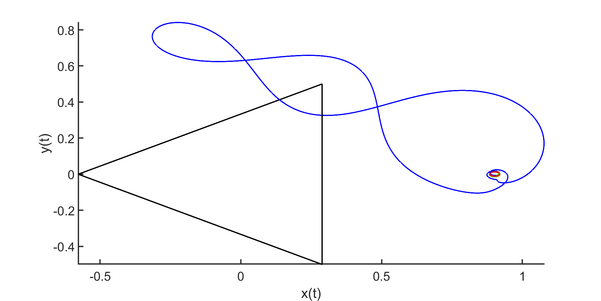
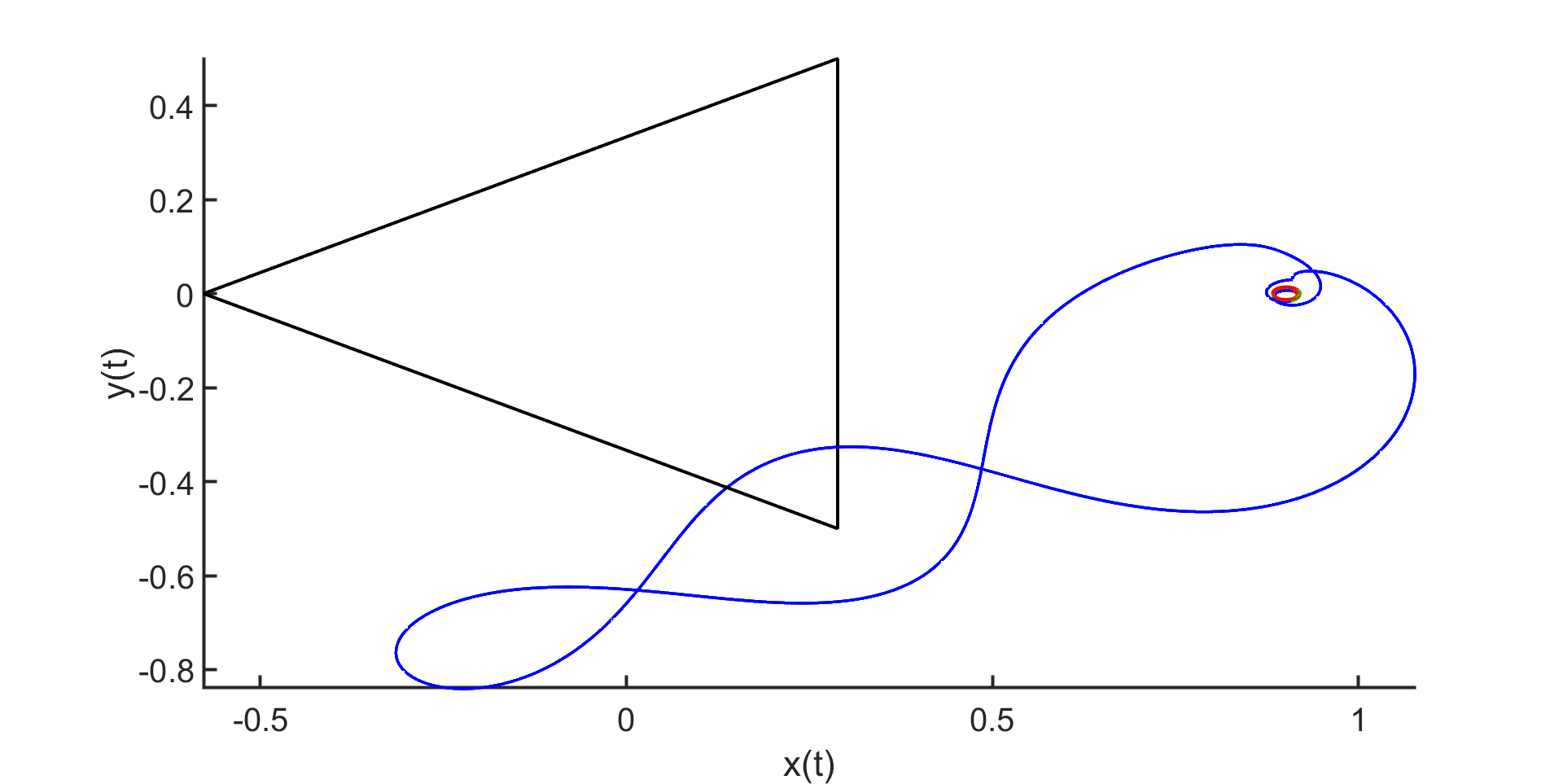
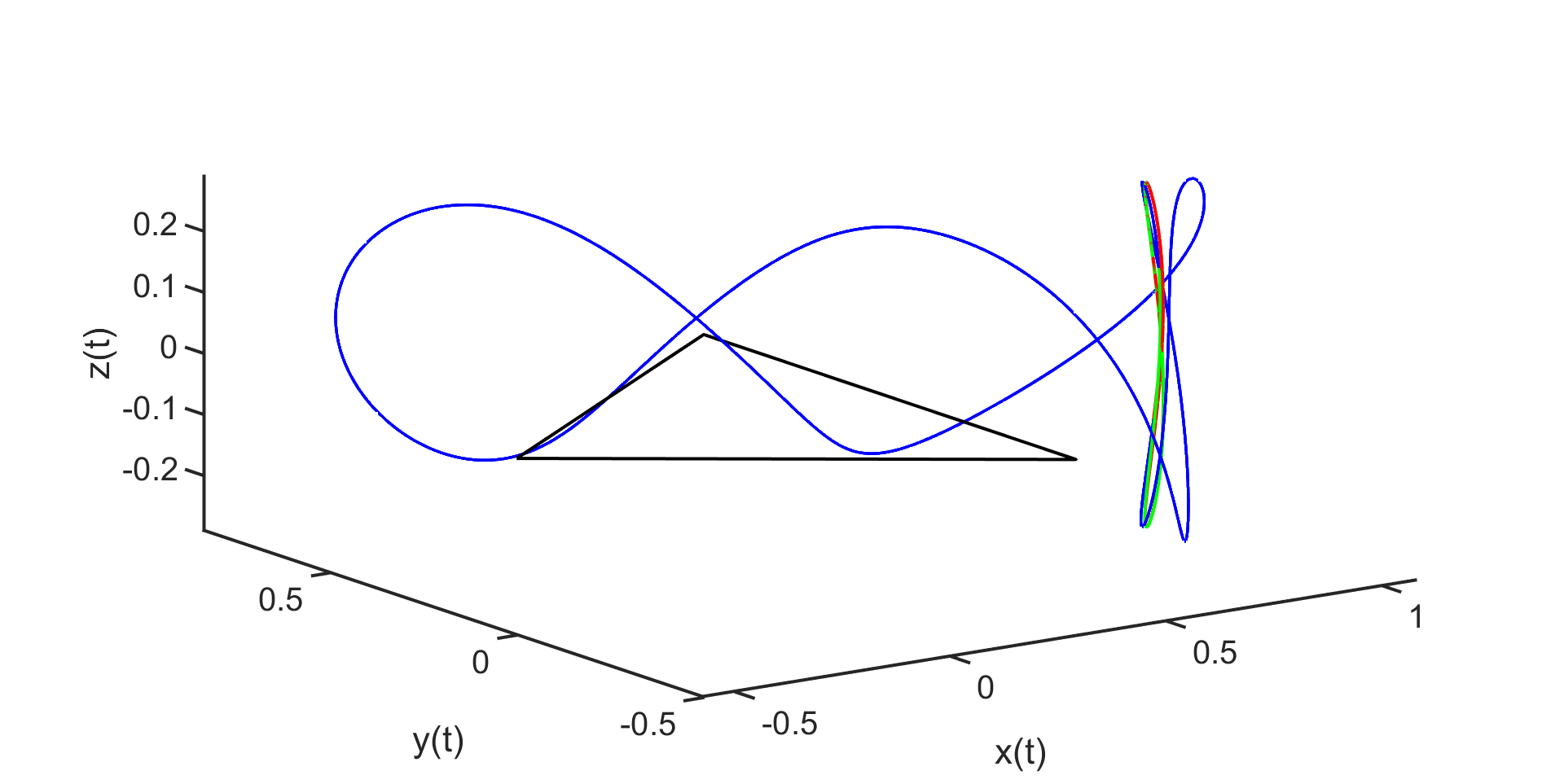
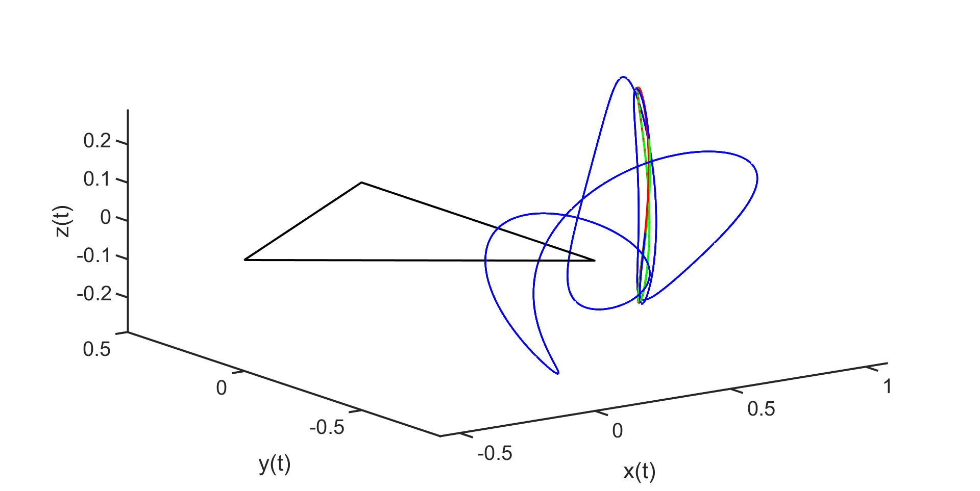
Figure 3: Two homoclinic connections with non-trivial winding about a primary, for a spatial periodic orbit in the vertical Lyapunov family at $\mathcal{L}_{5}$ in the triple Copenhagen problem. The top row displays the projection in the $x-y$ plane, while the bottom row illustrates the $x-y-z$ projection. Notice from the second angle that both connections are indeed out of plane. Each of the connections is validated using Theorem 2.11, so that a true solution lays in a neighborhood of the approximation displayed. The size of the neighborhood in the $C^{0}$ norm is specified for each case in Theorem 5.1. The Jacobi constant for these cycle-to-cycle connections is approximately $2.84$.

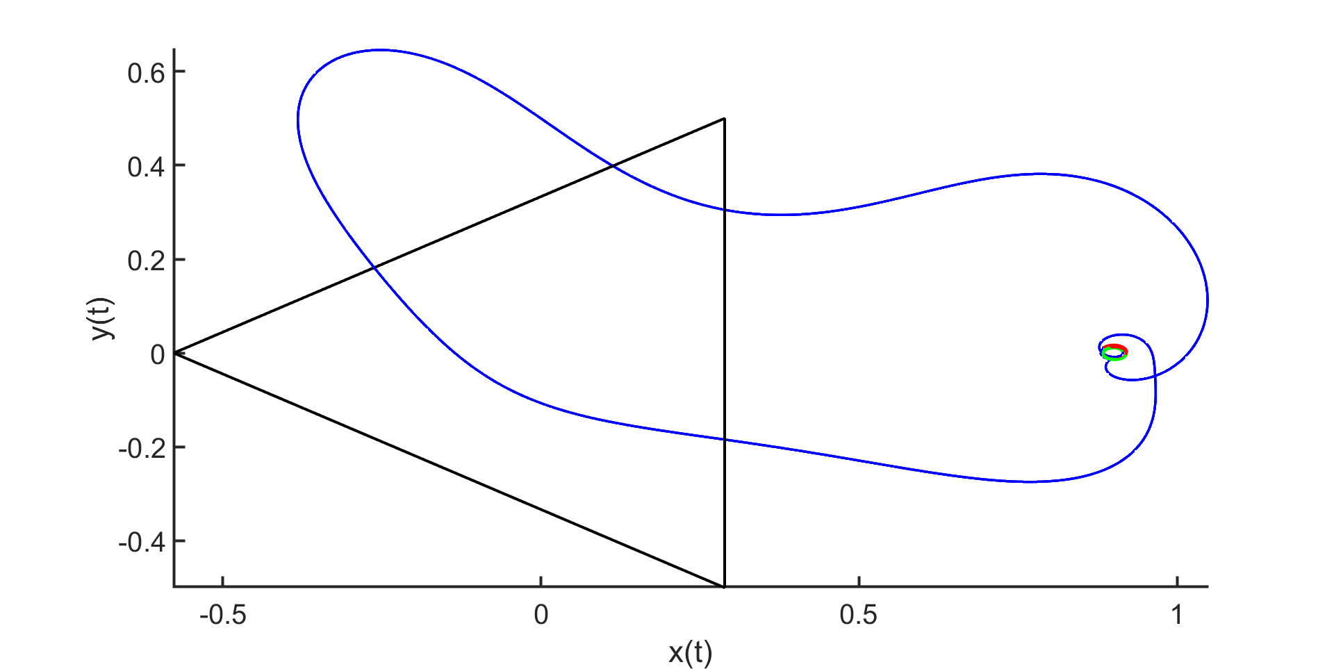
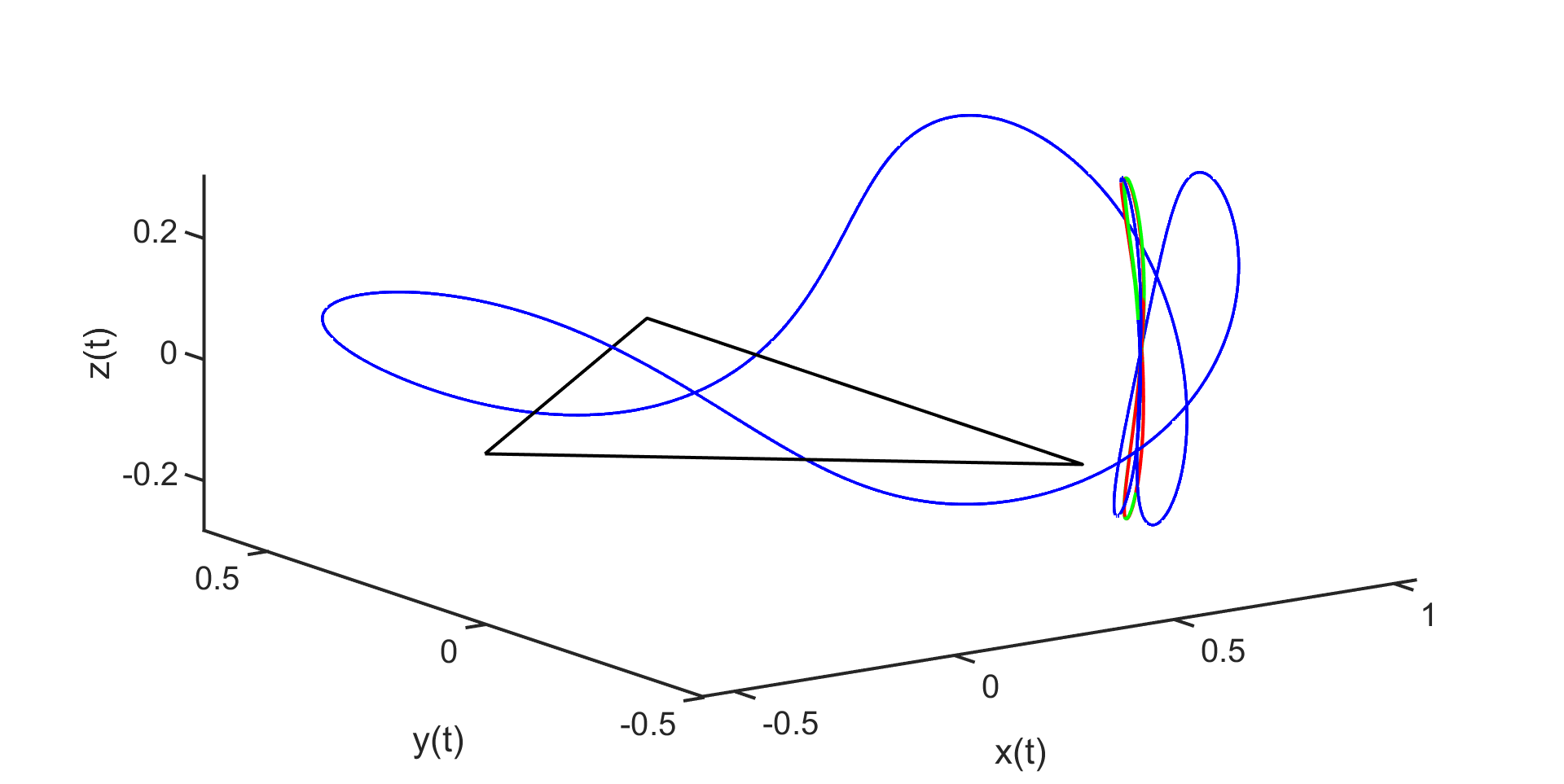
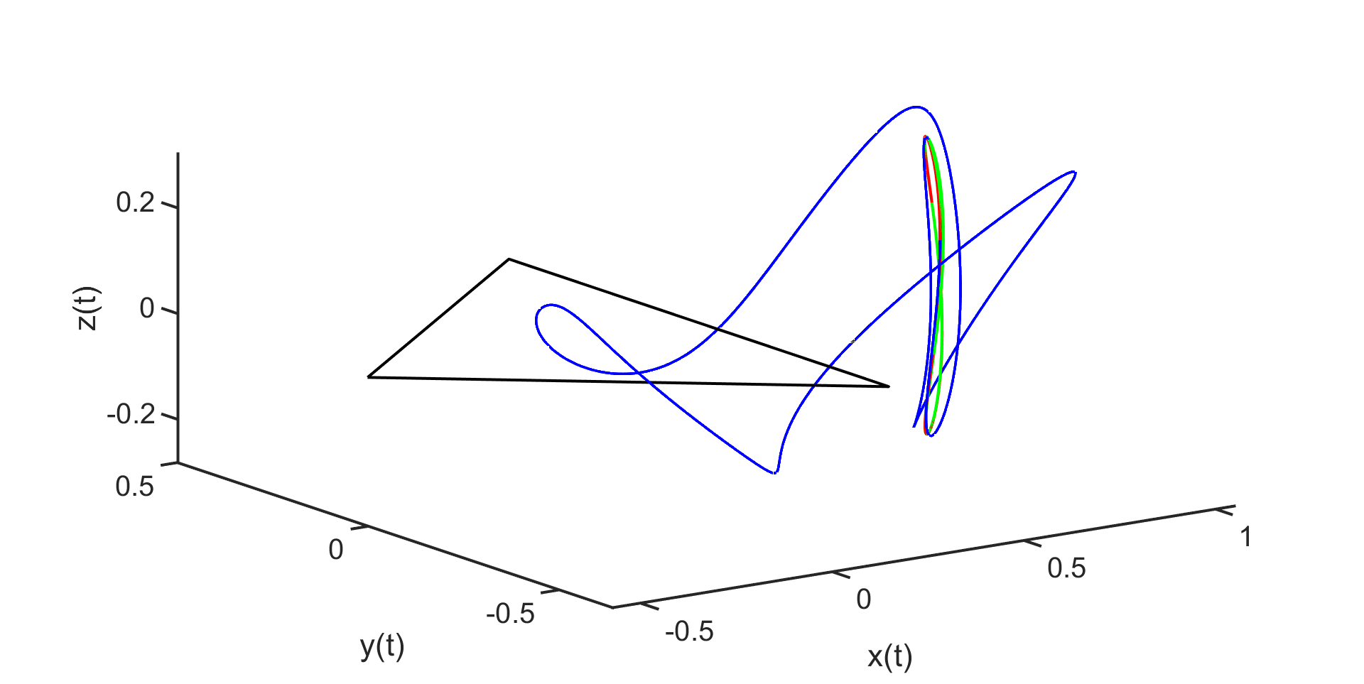
Figure 4: Homoclinic connections with trivial winding about all three primary bodies, for a spatial periodic orbit in the vertical Lyapunov family at $\mathcal{L}_{5}$ in the triple Copenhagen problem. Note that the connections pass through the “inner system”, i.e. through the equilateral triangle formed by the primaries. Error bounds are as given in Theorem 5.1, and projections displayed and energies are as described in the caption of Figure 3

Theorem 5.1 (Transverse spatial homoclinics for a Lyapunov orbit at $\mathcal{L}_{5}$ in the Triple Copenhagen problem).

There exists a spatial periodic orbit $\gamma$ in the Triple Copenhagen problem with 2D stable and 2D unstable attached local invariant manifolds. The Jacobi constant for $\gamma$ is approximately $2.84$. Moreover, there exist six distinct transverse homoclinic connections for $\gamma$ in the same energy level. The connections are illustrated in Figures 3, 4 and 5.

The computation are performed with $K=30$ Fourier modes, and $N_{t}=6$ Taylor modes for the parameterized manifolds. The scale of the eigenfunctions are controlled by taking phase conditions as in Equation (22) with $k_{0}=10$ and $\xi_{0}=10^{-5}$. The parameterized local stable manifold $P$, and local unstable manifold $Q$ satisfy

$$\left\|P-\bar{P}\right\|_{\infty} \leq 1.076\cdot 10^{-12},\leavevmode\nobreak\ \mbox{and}$$

$$\left\|Q-\bar{Q}\right\|_{\infty} \leq 1.597\cdot 10^{-12}.$$

These parameterizations are used to set up BVPs (36) for all six connecting orbits. We numerically compute approximate solutions $\bar{v}_{a},\bar{v}_{b},\bar{v}_{c},\bar{v}_{d},\bar{v}_{e},\bar{v}_{f}$ displayed in Figures 3, 4 and 5. Applying Theorem 2.11, we obtain the existence of true solutions having

$$\left\|v_{a}-\bar{v}_{a}\right\|_{\infty} \leq 5.155\cdot 10^{-9},$$

$$\left\|v_{b}-\bar{v}_{b}\right\|_{\infty} \leq 5.108\cdot 10^{-9},$$

$$\left\|v_{c}-\bar{v}_{c}\right\|_{\infty} \leq 3.074\cdot 10^{-9},$$

$$\left\|v_{d}-\bar{v}_{d}\right\|_{\infty} \leq 2.636\cdot 10^{-9},$$

$$\left\|v_{e}-\bar{v}_{e}\right\|_{\infty} \leq 1.626\cdot 10^{-8},\leavevmode\nobreak\ \mbox{and}$$

$$\left\|v_{f}-\bar{v}_{f}\right\|_{\infty} \leq 1.936\cdot 10^{-8},$$

in the $C^{0}$ norm. The proofs for $v_{a}$ and $v_{b}$ are formulated with $M=9$ Chebyshev domains, each with $50$ non-zero coefficients. The remaining proofs are formulated with $M=8$ domains and $45$ Chebyshev coefficients.

Theorem 5.2 (Error bound of solutions at $\mathcal{L}_{0}$).

There exists a spatial periodic orbit $\gamma$ in the CRFBP with $m_{1}=0.4$, $m_{2}=0.33$, and $m_{3}=0.27$. The cycle $\gamma$ has 2D stable and 2D unstable attached local invariant manifolds. The Jacobi constant for $\gamma$ is approximately $3.26$. Moreover, there exist six distinct transverse homoclinic connections for $\gamma$. The connections are illustrated in Figure 6.

These computation where performed with $K=30$ Fourier and $N_{t}=6$ Taylor modes for the parameterization of each manifold, and scalings set (as in Equation (22)) with $k_{0}=10$ and $\xi_{0}=10^{-4}$. The parameterized stable manifold $P$, and unstable manifold $Q$ satisfy

$$\left\|P-\bar{P}\right\|_{\infty} \leq 2.154\cdot 10^{-12},\leavevmode\nobreak\ \mbox{and}$$

$$\left\|Q-\bar{Q}\right\|_{\infty} \leq 1.679\cdot 10^{-12}.$$

These parameterization are used to set up BVPs (36) for all six connections. We use Netwon’s method to compute approximated solutions $\bar{v}_{a},\bar{v}_{b},\bar{v}_{c},\bar{v}_{d},\bar{v}_{e},\bar{v}_{f}$ displayed in Figure 6. Again, using Theorem 2.11 we obtain that

$$\left\|v_{a}-\bar{v}_{a}\right\|_{\infty} \leq 1.999\cdot 10^{-9},$$

$$\left\|v_{b}-\bar{v}_{b}\right\|_{\infty} \leq 2.504\cdot 10^{-9},$$

$$\left\|v_{c}-\bar{v}_{c}\right\|_{\infty} \leq 1.885\cdot 10^{-9},$$

$$\left\|v_{d}-\bar{v}_{d}\right\|_{\infty} \leq 4.763\cdot 10^{-9},$$

$$\left\|v_{e}-\bar{v}_{e}\right\|_{\infty} \leq 3.027\cdot 10^{-9},\leavevmode\nobreak\ \mbox{and}$$

$$\left\|v_{f}-\bar{v}_{f}\right\|_{\infty} \leq 3.591\cdot 10^{-9}.$$

The short connections (displayed on the left of Figure 6) are computed with $M=4$ Chebyshev domains, each with $40$ non-zero coefficients. The longer connections (displayed on the right of Figure 6) are computed with $M=8$ Chebyshev domains, each with $50$ non-zero coefficients.

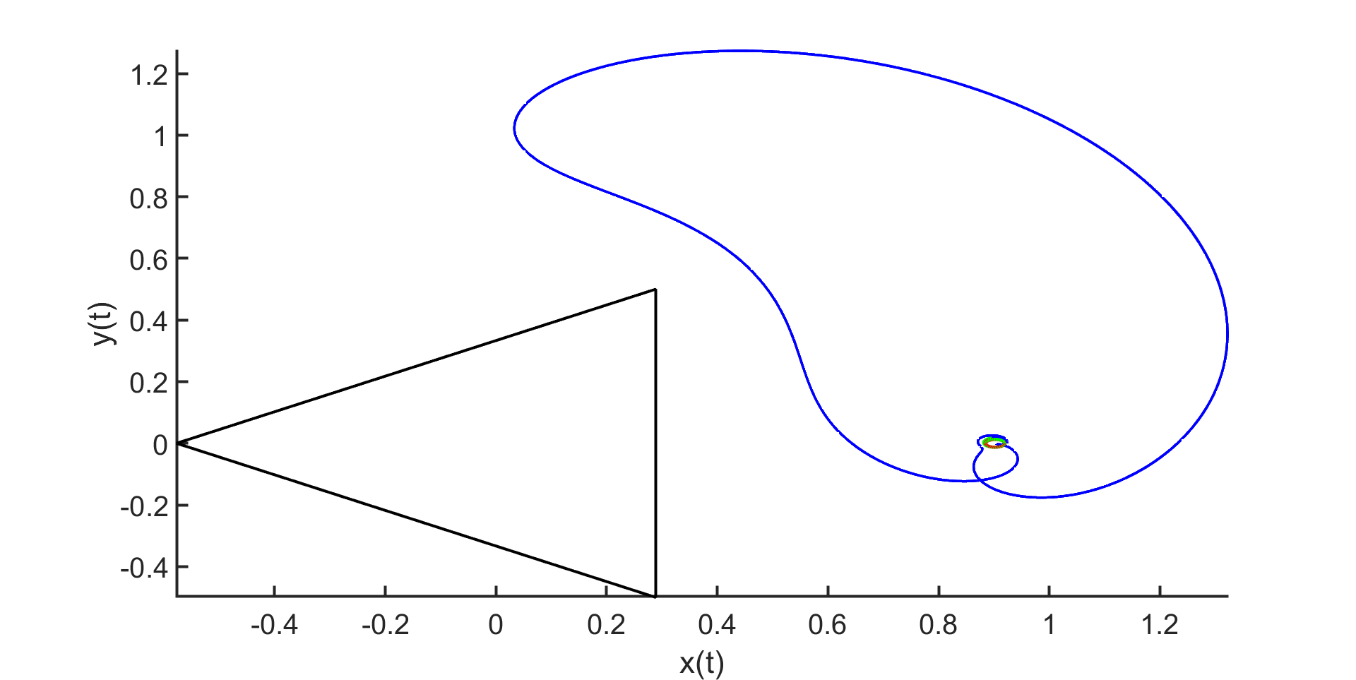
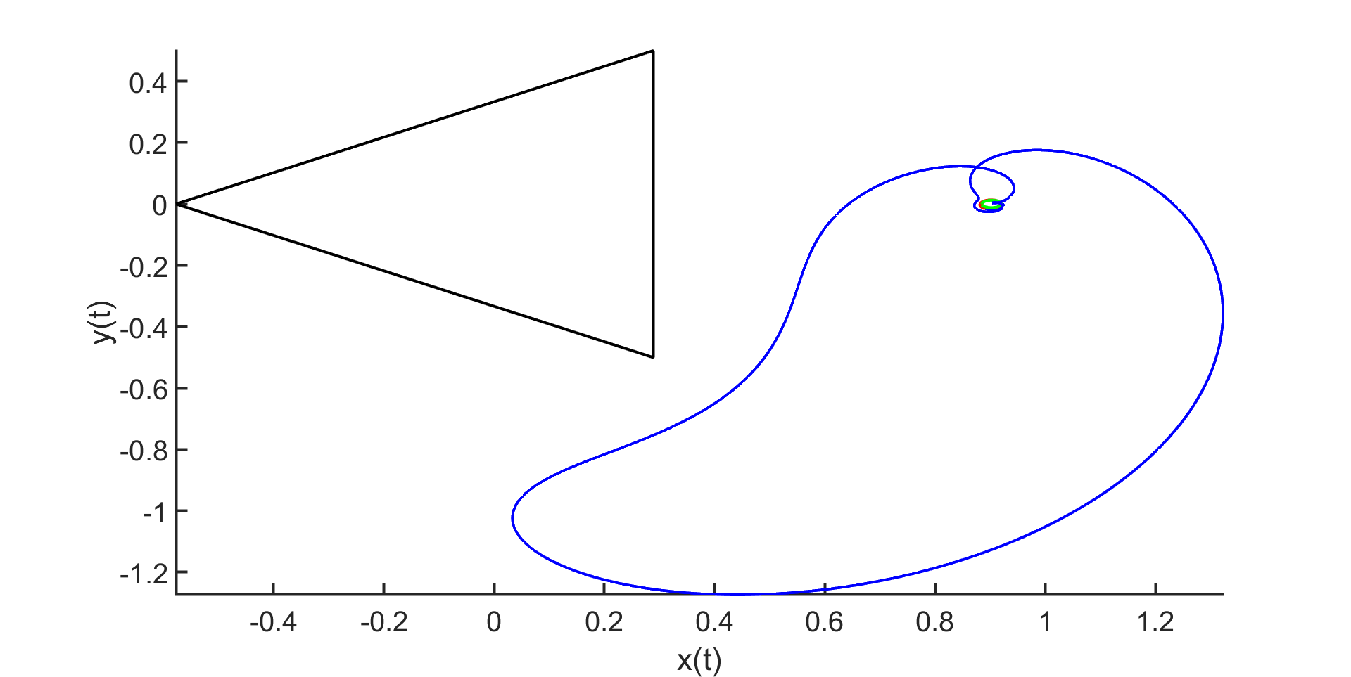
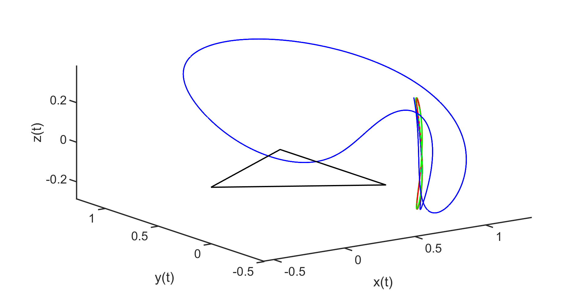
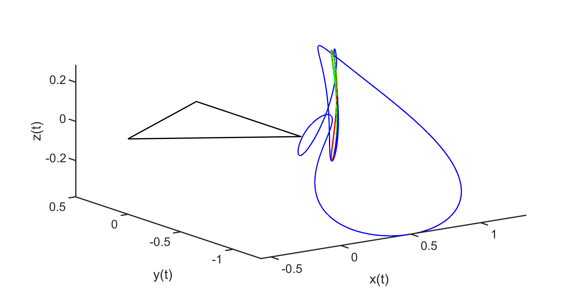
Figure 5: Homoclinic connections with trivial winding about all three primary bodies, for a spatial periodic orbit in the vertical Lyapunov family at $\mathcal{L}_{5}$ in the triple Copenhagen problem. Note that the connections are entirely in the “outer system”, i.e. the orbits do not intersect the equilateral triangle formed by the primaries. Error bounds are as given in Theorem 5.1, and projections displayed and energies are as described in the caption of Figure 3

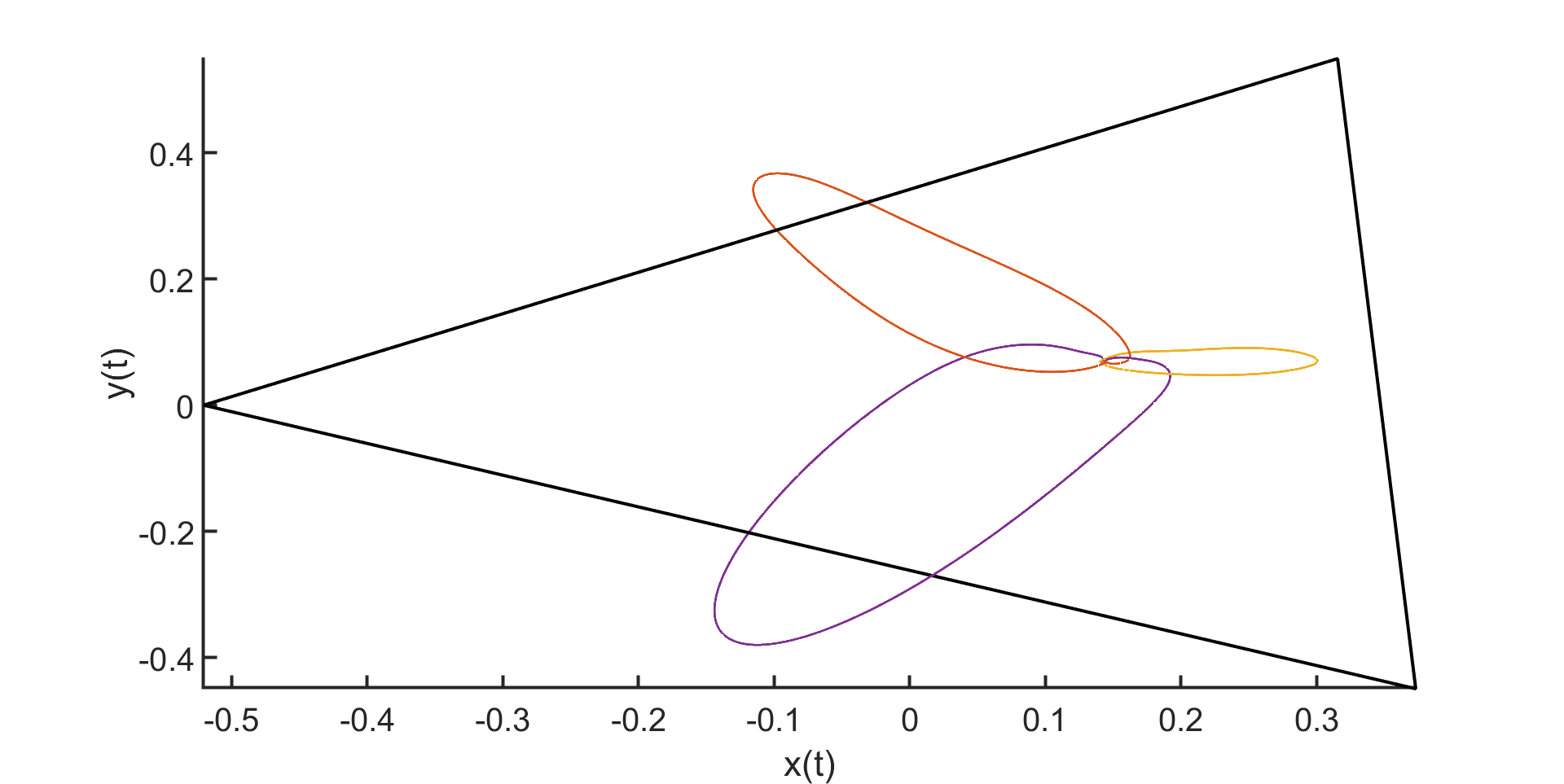
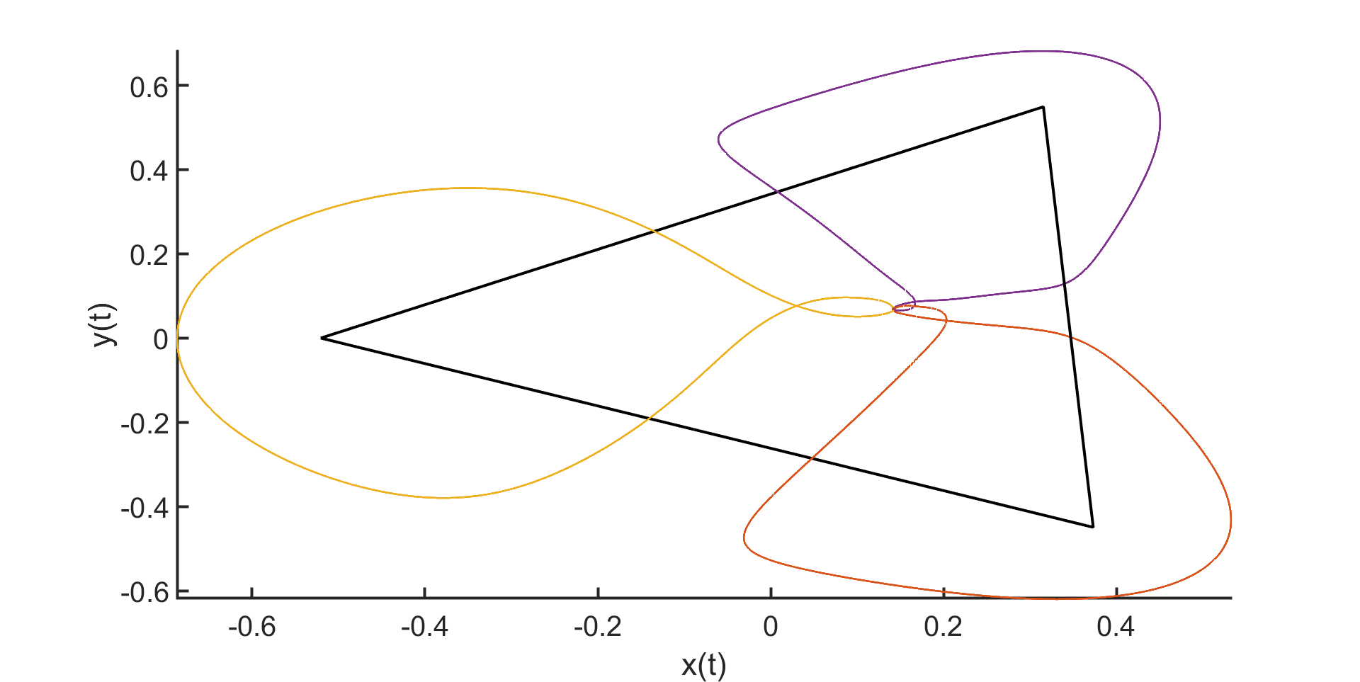
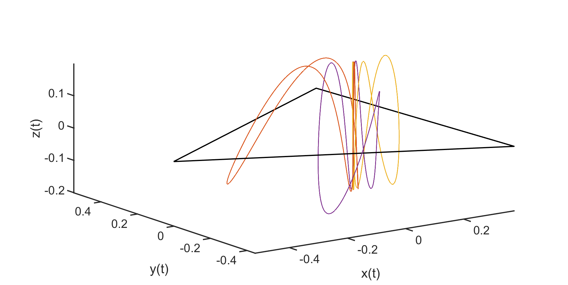
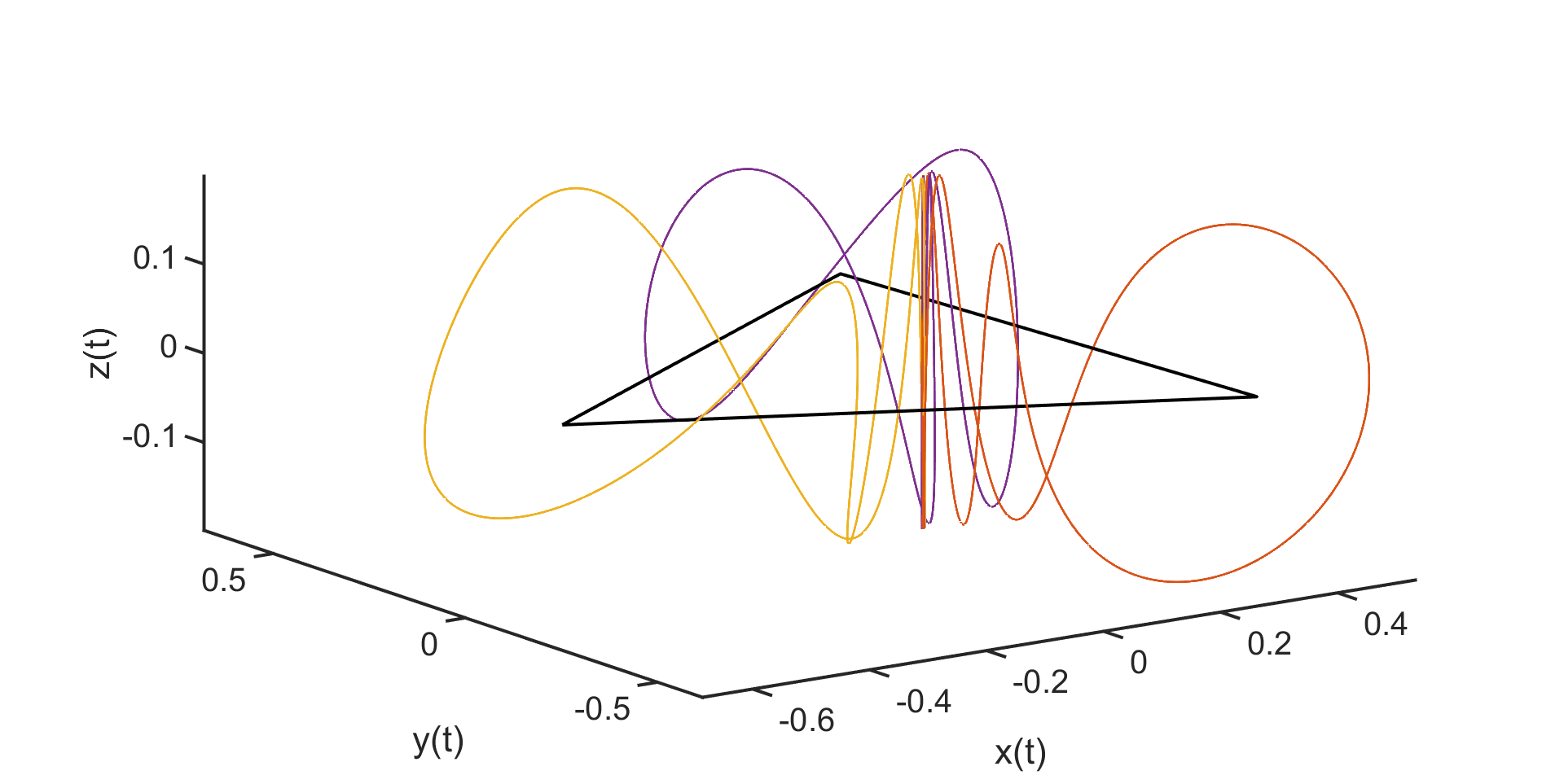
Figure 6: Homoclinic connections to a spatial periodic orbit from the vertical Lyapunov family at $\mathcal{L}_{0}$ with $m_{1}=0.4$, $m_{2}=0.33$, and $m_{3}=0.27$. The first row displays the connection seen from above, while the bottom row exhibits that the connections are indeed out of plane. Each of the connections has been validated with the help of Theorem 2.11, so that a true solution lays in a neighborhood of the approximation displayed. The size of said neighborhood, thus a bound on the $C^{0}$ norm, is specified for each case in Theorem 5.2. The computation were executed with a fixed frequency for the periodic orbit, hence the exact energy isn’t provided by the validation algorithm. We note however that the energy is of approximately $3.26$.

Appendix A Cauchy Bounds for analytic functions: Fourier and Taylor cases

The following lemmas facilitate control of all necessary partial derivatives the the Fourier-Taylor series appearing in our computer assisted proofs. The quite standard proofs are included for the sake of completeness.

Lemma A.1 (Bounds for Analytic Functions given by Fourier Series).

Suppose that $\{a_{n}\}_{n\in\mathbb{Z}}$ is a two sided sequence of complex numbers, that $\omega>0$, and that $\|a\|_{1,\nu}<\infty$, for some $\nu>1$. Let

$$f(z):=\sum_{n\in\mathbb{Z}}a_{n}e^{i\omega kz}.$$

For $r>0$ let

$$A_{r}:=\{z\in\mathbb{C}\,|\,|\mbox{{\em imag}}(z)|<r\},$$

denote the open complex strip of width $r$.

• $\ell_{\nu}^{1}$ bounds imply $C^{0}$ bounds: The function $f$ is analytic on the strip $A_{r}$ with $r=\ln(\nu)/\omega$, continuous on the closure of $A_{r}$, and satisfies

  $$\sup_{z\in A_{r}}|f(z)|\leq\|a\|_{1,\nu}.$$

  Moreover $f$ is $T$-periodic with $T=2\pi/\omega$.

• Cauchy Bounds: Let $0<\sigma<r$ and

  $$\tilde{\nu}=e^{\omega(r-\sigma)}.$$

  Define the sequence $b=\{b_{n}\}_{n\in\mathbb{Z}}$ by

  $$b_{n}=i\omega na_{n}.$$

  Then

  $$\|b\|_{\tilde{\nu}}^{1}\leq\frac{1}{e\sigma}\|a\|_{1,\nu},$$

  and

  $$\sup_{z\in A_{r-\sigma}}|f^{\prime}(z)|\leq\frac{1}{e\sigma}\|a\|_{1,\nu}.$$

Proof.

For $\nu>1$, let $r=\ln(\nu)/\omega$ (i.e. $\nu=e^{\omega r}$) and consider $z\in A_{r}$. We have that

$$|f(z)| \leq\sum_{n\in\mathbb{Z}}|a_{n}|\left|\left(e^{i\omega z}\right)^{n}\right|$$

$$\leq\sum_{n\in\mathbb{Z}}|a_{n}|\left(e^{\omega\left|\mbox{imag}(z)\right|}\right)^{|n|}$$

$$\leq\sum_{n\in\mathbb{Z}}|a_{n}|\nu^{|n|}$$

$$=\|a\|_{1,\nu}.$$

It follows that $f$ is analytic as the Fourier series converges absolutely and uniformly in $A_{r}$. Continuity at the boundary of the strip also follows from the absolute summability of the series. From the fact that $f$ is analytic in $A_{r}$ it follows that the derivative $f^{\prime}(z)$ exists for any $z$ in the interior of $A_{r}$, and that

$$f^{\prime}(z)=\sum_{n\in\mathbb{Z}}i\omega na_{n}e^{i\omega nz}=\sum_{n\in\mathbb{Z}}b_{n}e^{i\omega nz}.$$

However the fact that $f$ is uniformly bounded on $A_{r}$ does not imply uniform bounds on $f^{\prime}$. Indeed it may be that $f^{\prime}$ has singularities at the boundary.

In order to obtain uniform bounds on the derivative we give up a portion of the width of the domain. More precisely we consider the supremum of $f^{\prime}$ on the strip $A_{r-\sigma}$ with $0<\sigma<r$. Letting $\nu=e^{\omega r}$, so that $\tilde{\nu}=e^{\omega(r-\sigma)}$, define the function $s\colon\mathbb{R}^{+}\to\mathbb{R}$ by

$$s(x):=x\alpha^{x},$$

with $\alpha=\tilde{\nu}/\nu=e^{-\omega\sigma}<1$. Note that $s(x)\geq 0$ for all $x\geq 0$, $s(0)=0$, and that $s(x)\to 0$ as $x\to\infty$. Moreover $s$ is bounded and attains its maximum at

$$\hat{x}=\frac{1}{\omega\sigma},$$

as can be seen by computing the critical point of $s$. It follows that

$$s(x)\leq s(\hat{x})=\frac{1}{e\omega\sigma}.$$

From this we have

$$\|b\|_{1,\tilde{\nu}} = \sum_{n\in\mathbb{Z}}|b_{n}|\tilde{\nu}^{|n|}$$

$$= \sum_{n\in\mathbb{Z}}\omega|n||a_{n}|\tilde{\nu}^{|n|}\frac{\nu^{|n|}}{\nu^{|n|}}$$

$$= \sum_{n\in\mathbb{Z}}\omega|n|\left(\frac{\tilde{\nu}}{\nu}\right)^{|n|}|a_{n}|\nu^{|n|}$$

$$= \sum_{n\in\mathbb{Z}}\omega s(|n|)|a_{n}|\nu^{|n|}$$

$$\leq \sum_{n\in\mathbb{Z}}\omega\frac{1}{e\omega\sigma}|a_{n}|\nu^{|n|}$$

$$= \frac{1}{e\sigma}\|a\|_{1,\nu}.$$

It follows by $(I)$ that if $z\in A_{r-\sigma}$ then

$$|f^{\prime}(z)|\leq\|b\|_{1,\tilde{\nu}}\leq\frac{1}{e\sigma}\|a\|_{1,\nu},$$

as desired. ∎

Lemma A.2 (Bounds for Analytic Functions given by Taylor Series).

Let $\nu>0$ and suppose that $\{a_{n}\}_{n\in\mathbb{N}}$ is a one sided sequence of complex numbers with

$$\|a\|_{1,\nu}=\sum_{n=0}^{\infty}|a_{n}|\nu^{n}<\infty.$$

Define

$$f(z):=\sum_{n=0}^{\infty}a_{n}z^{n},$$

and let

$$D_{\nu}:=\{z\in\mathbb{C}\,|\,|z|<\nu\},$$

denote the complex disk of radius $\nu>0$ centered at the origin.

• $\ell_{\nu}^{1}$ bounds imply $C^{0}$ bounds: The function $f$ is analytic on the disk $D_{\nu}$, continuous on the closure of $D_{\nu}$, and satisfies

  $$\sup_{z\in D_{\nu}}|f(z)|\leq\|a\|_{1,\nu}.$$

• Cauchy Bounds: Let $0<\sigma\leq 1$ and

  $$\tilde{\nu}=\nu e^{-\sigma}.$$

  Then

  $$\sup_{z\in D_{\tilde{\nu}}}|f^{\prime}(z)|\leq\frac{1}{\nu\sigma}\|a\|_{1,\nu}.$$

Proof.

The proof is similar to the proof of Lemma A.1, the difference being the estimate of the derivative. Since $f$ is analytic in $D_{\nu}$ we have

$$f^{\prime}(z)=\sum_{n=1}^{\infty}na_{n}z^{n-1},$$

for all $z\in B_{\nu}$, and again we will trade some domain for uniform bounds on derivatives. So, choose $0<\sigma\leq 1$ and define $\tilde{\nu}=\nu e^{-\sigma}$. As in the Fourier case, define the function $s\colon[0,\infty)\to\mathbb{R}$ by

$$s(x):=xe^{-\sigma x}.$$

We have that $s$ is positive and

$$s(x)\leq\frac{1}{e\sigma}.$$

Then for any $z\in D_{\tilde{\nu}}$ we have

$$|f^{\prime}(z)| = \sum_{n=1}^{\infty}n|a_{n}||z|^{n-1}$$

$$\leq \sum_{n=1}^{\infty}n|a_{n}|\frac{\nu}{\nu}|\nu e^{-\sigma}|^{n-1}$$

$$\leq \sum_{n=1}^{\infty}\left(\frac{e^{\sigma}}{\nu}ne^{-\sigma n}\right)|a_{n}|\nu^{n}$$

$$\leq \sum_{n=1}^{\infty}\left(\frac{e}{\nu}ne^{-\sigma n}\right)|a_{n}|\nu^{n}$$

$$\leq \sum_{n=0}^{\infty}\frac{e}{\nu}s(n)|a_{n}|\nu^{n}$$

$$\leq \sum_{n=0}^{\infty}\frac{e}{\nu}\frac{1}{e\sigma}|a_{n}|\nu^{n}$$

$$= \frac{1}{\nu\sigma}\|a\|_{1,\nu}^{1}.$$

∎

We now to consider these lemmas to the context of parameterized periodic manifolds for the CRFBP. Let $\omega_{m}$ denote the Frequency of the periodic orbit of interest, and $\nu_{m}$ denote the weight taken for the $\ell_{\nu}^{1}$ norms from each step of the validation discussed in Section 4. The weight in the Taylor direction is $1$ by construction of the norm in $X_{2}^{\infty}$. Lemma is A.2 is applied with $\nu=1$, for fixed $r^{\star}$, to the endpoint of the domain of the polynomial bound in Theorem 2.11. Choose $\sigma_{m}$ such that

$$r^{\star}<\frac{\ln(\nu_{m})}{\omega_{m}}-\sigma_{m}.$$

It follows that for all radius $r\leq r^{\star}$ and for $b\in\mathbb{R}$ with $|b|=r$, we have that

$$\left\|\frac{\partial}{\partial\theta}E(\bar{\theta},\bar{\phi})b\right\|_{\infty}=\max_{1\leq i\leq 9}\left|\frac{\partial}{\partial\theta}E^{i}(\bar{\theta},\bar{\phi})b\right|\leq\left(\frac{r_{m}}{e\sigma_{m}}\right)r.$$ (45)

The other partial derivative is bound similarly, and it follows from the chain rule that

$$\frac{\partial}{\partial\phi}E(\bar{\theta},\bar{\phi}) =\frac{\partial}{\partial\sigma_{1}}E(\bar{\theta},\bar{\sigma}_{1},\bar{\sigma}_{2})\frac{\partial\sigma_{1}}{\partial\phi}+\frac{\partial}{\partial\sigma_{2}}E(\bar{\theta},\bar{\sigma}_{1},\bar{\sigma}_{2})\frac{\partial\sigma_{2}}{\partial\phi},$$

where $\frac{\partial\sigma_{1}}{\partial\phi}$ and $\frac{\partial\sigma_{2}}{\partial\phi}$ depend on the choice of the function $\sigma(\rho,\phi)=(\sigma_{1},\sigma_{2})$. Note however that in this work, the partial derivatives of interest are bounded by a constant $\rho$ that can be fixed in the construction of the BVP. Again, Lemma A.2 is applied with $\nu=1$ as the weight in the Taylor direction. Hence, whenever $\rho$ satisfies

$$\rho<\tilde{\nu}=e^{\ln(0.99)}\,\stackrel{{\scriptstyle\mbox{\tiny{\raisebox{0.0pt}[0.0pt][0.0pt]{def}}}}}{{=}}\,e^{-s}$$

it follows that

$$\left\|\frac{\partial}{\partial\phi}E(\bar{\theta},\bar{\phi})b\right\|_{\infty}\leq\left(2\rho\frac{r_{m}}{s}\right)r,$$ (46)

for any $\|b\|_{\infty}=r$. Finally, note that whenever $\rho_{u}$ is a variable of the problem it is possible to use Lemma A.2 to obtain

$$\left\|\frac{\partial}{\partial\rho_{u}}E(\bar{\theta},\bar{\phi})b\right\|_{\infty}\leq\left(2\frac{r_{m}}{s}\right)r.$$ (47)

This follows from the chain rule, and we note that this estimates require that $L$ is fixed large enough so that $\bar{\rho}_{u}+r<\tilde{\nu}$. This verification ensures the validity of the estimates in a neighborhood of the approximation. The variable $\rho_{s}$ is fixed and the stable parameterization will not require this last estimate.

Appendix B Numerical bounds on the norms of each $D_{ij}^{\infty}$

It was already shown in Section 3.4 that

$$\left\|\mathcal{L}_{\alpha}^{-1}\circ D^{\infty}(h)\right\|_{(\ell_{\nu}^{1})^{9}} \leq\max_{1\leq i\leq 9}\sum_{|k|<K}\left|\frac{\left(D^{\infty}h\right)_{k}^{i}}{-\mathrm{i}\omega k-\langle\alpha,\lambda\rangle}\right|\nu^{|k|}+d_{\alpha}^{\infty}\sum_{j=1}^{9}\left\|D_{ij}^{\infty}\right\|_{\mathcal{B}\left(\ell_{\nu}^{1}\right)}$$

The cases $i=1,3,5$ include only a single linear term, and is non-zero only in the case $|k|\geq K$, so that the first sum vanishes in these cases and we set

$$\|D_{12}^{\infty}\|_{\mathcal{B}(\ell_{\nu}^{1})}=\|D_{34}^{\infty}\|_{\mathcal{B}(\ell_{\nu}^{1})}=\|D_{35}^{\infty}\|_{\mathcal{B}(\ell_{\nu}^{1})}=1.$$

The other cases contain convolution products. For example, for all $k\in\mathbb{Z}$ we have that

$$(D_{21}^{\infty}h^{1})_{k} =\sum_{i=1}^{3}m_{i}\left[(h^{\infty})^{1}\star(a_{0}^{K})^{6+i}\star(a_{0}^{K})^{6+i}\star(a_{0}^{K})^{6+i}\right]_{k}+3m_{i}\left[h^{1}\star(a_{0}^{\infty})^{6+i}\star(a_{0}^{K})^{6+i}\star(a_{0}^{K})^{6+i}\right]_{k}$$

$$+\sum_{i=1}^{3}3m_{i}\left[h^{1}\star(a_{0}^{\infty})^{6+i}\star(a_{0}^{\infty})^{6+i}\star(a_{0}^{K})^{6+i}\right]_{k}+m_{i}\left[h^{1}\star(a_{0}^{\infty})^{6+i}\star(a_{0}^{\infty})^{6+i}\star(a_{0}^{\infty})^{6+i}\right]_{k}$$

To compute a bound on this term, we note that

$$\|(a_{0}^{K})^{i}\|_{1,\nu}\leq\|\bar{a}_{0}^{i}\|_{1,\nu}+r_{0}\,\stackrel{{\scriptstyle\mbox{\tiny{\raisebox{0.0pt}[0.0pt][0.0pt]{def}}}}}{{=}}\,n^{i},\quad\forall i=1,2,\ldots,9,$$

so that

$$\left\|D_{21}^{\infty}h^{1}\right\|_{1,\nu}\leq\sum_{i=1}^{3}\left[\sum_{|k|<K}\left|\left[(h^{\infty})^{1}\star(a_{0}^{K})^{6+i}\star(a_{0}^{K})^{6+i}\star(a_{0}^{K})^{6+i}\right]_{k}\right|\nu^{|k|}+3m_{i}r_{0}n^{6+i}n^{6+i}+3m_{i}r_{0}r_{0}n^{6+i}+m_{i}r_{0}r_{0}r_{0}\right].$$

Appendix C The $Z_{1}$ bound for Chebyshev expansion

In this section we present a table containing bounds for all non-zero terms in the $Z_{1}$ estimates. Throughout the discussion, $h^{i,j}$ denotes an element of $\ell_{\nu}^{1}$ with norm $r$ and $h^{i,j}_{\infty}=h^{i,j}-\pi_{m}{h^{i,j}}$, so that $(h^{i,j}_{\infty})_{k}=0$ for $k<m-1$. Recall also that $\bar{a}^{i,j}$ is the $i-$th component of the $j-$th sequence of Chebyshev coefficients of the solution to (36). Some $d^{i}$ are simplified due to the fact that that we always choose $\bar{\beta}=0$. Then any terms which are constant or higher order with respect to $\beta$ do not appear in the derivatives, and hence are not present in the bounds (only first order terms with respect to $\beta$ are present).

For the sake of completeness, one case is illustrated. Consider

$$d_{k}^{2,j}= \Lambda_{k}\left(h_{l}\left(\bar{\beta}\bar{a}^{2,j}+2\bar{a}^{4,j}+\bar{a}^{1,j}\right)+\bar{L}\left(h_{\beta}\bar{a}^{2,j}+\bar{\beta}h^{2,j}+2h^{4,j}+h^{1,j}\right)\right)$$

$$+h_{L}\Lambda_{k}\left(\sum_{j=1}^{3}m_{j}(\bar{a}^{1,j}-x_{1})\ast\bar{a}^{6+i,j}\ast\bar{a}^{6+i,j}\ast\bar{a}^{6+i,j}\right)$$

$$+\bar{L}\Lambda_{k}\left(\sum_{l=1}^{3}m_{j}\left(h^{1,j}\ast\bar{a}^{6+l,j}\ast\bar{a}^{6+l,j}\ast\bar{a}^{6+l,j}+3(\bar{a}^{1,j}-x_{l})\ast h^{6+l,j}\ast\bar{a}^{6+l,j}\ast\bar{a}^{6+l,j}\right)\right)$$

Finally, note that all other cases are zero. So that the six scalar components are zero, and $d_{0}^{i,j}=0$ for all $1\leq i\leq 9$, $1\leq j\leq M$. The other cases are in the two tables.

Table 1: The sequence $d\in X$ for all $1\leq j\leq M$, cases $1\leq i\leq 6$

$i$ and $k$	$d_{k}^{6+9(j-1)+i}$
$1$, $1\leq k<m$	$0$
$1$, $k\geq m$	$\bar{L}\Lambda_{k}(h^{2,j})$
$2$, $1\leq k<m$	$\bar{L}\displaystyle\sum_{l=1}^{3}m_{l}\Lambda_{k}\left(h^{1,j}_{\infty}\ast\bar{a}^{6+l,j}\ast\bar{a}^{6+l,j}\ast\bar{a}^{6+l,j}+3(\bar{a}^{1,j}-x_{l})\ast h^{6+l,j}_{\infty}\ast\bar{a}^{6+l,j}\ast\bar{a}^{6+l,j}\right)$
$2$, $k\geq m$	$\bar{L}\Lambda_{k}(2h^{4,j}+h^{1,j})+h_{L}\Lambda_{k}\left(\displaystyle\sum_{j=1}^{3}m_{j}(\bar{a}^{1,j}-x_{1})\ast\bar{a}^{6+i,j}\ast\bar{a}^{6+i,j}\ast\bar{a}^{6+i,j}\right)$
	$+\bar{L}\Lambda_{k}\left(\displaystyle\sum_{l=1}^{3}m_{j}\left(h^{1,j}\ast\bar{a}^{6+l,j}\ast\bar{a}^{6+l,j}\ast\bar{a}^{6+l,j}+3(\bar{a}^{1,j}-x_{l})\ast h^{6+l,j}\ast\bar{a}^{6+l,j}\ast\bar{a}^{6+l,j}\right)\right)$
$3$, $1\leq k<m$	$0$
$3$, $k\geq m$	$\bar{L}\Lambda_{k}(h^{4,j})$
$4$, $1\leq k<m$	$\bar{L}\displaystyle\sum_{l=1}^{3}m_{l}\Lambda_{k}\left(h^{3,j}_{\infty}\ast\bar{a}^{6+l,j}\ast\bar{a}^{6+l,j}\ast\bar{a}^{6+l,j}+3(\bar{a}^{3,j}-y_{l})\ast h^{6+l,j}_{\infty}\ast\bar{a}^{6+l,j}\ast\bar{a}^{6+l,j}\right)$
$4$, $k\geq m$	$\bar{L}\Lambda_{k}(-2h^{2,j}+h^{3,j})+h_{L}\Lambda_{k}\left(\displaystyle\sum_{j=1}^{3}m_{j}(\bar{a}^{3,j}-y_{1})\ast\bar{a}^{6+i,j}\ast\bar{a}^{6+i,j}\ast\bar{a}^{6+i,j}\right)$
	$+\bar{L}\Lambda_{k}\left(\displaystyle\sum_{l=1}^{3}m_{j}\left(h^{3,j}\ast\bar{a}^{6+l,j}\ast\bar{a}^{6+l,j}\ast\bar{a}^{6+l,j}+3(\bar{a}^{3,j}-y_{l})\ast h^{6+l,j}\ast\bar{a}^{6+l,j}\ast\bar{a}^{6+l,j}\right)\right)$
$5$, $1\leq k<m$	$0$
$5$, $k\geq m$	$\bar{L}\Lambda_{k}(h^{6,j})$
$6$, $1\leq k<m$	$\bar{L}\displaystyle\sum_{l=1}^{3}m_{l}\Lambda_{k}\left(h^{5,j}_{\infty}\ast\bar{a}^{6+l,j}\ast\bar{a}^{6+l,j}\ast\bar{a}^{6+l,j}+3(\bar{a}^{5,j}-z_{l})\ast h^{6+l,j}_{\infty}\ast\bar{a}^{6+l,j}\ast\bar{a}^{6+l,j}\right)$
$6$, $k\geq m$	$h_{L}\Lambda_{k}\left(\displaystyle\sum_{j=1}^{3}m_{j}(\bar{a}^{5,j}-z_{1})\ast\bar{a}^{6+i,j}\ast\bar{a}^{6+i,j}\ast\bar{a}^{6+i,j}\right)$
	$+\bar{L}\Lambda_{k}\left(\displaystyle\sum_{l=1}^{3}m_{j}\left(h^{5,j}\ast\bar{a}^{6+l,j}\ast\bar{a}^{6+l,j}\ast\bar{a}^{6+l,j}+3(\bar{a}^{5,j}-z_{l})\ast h^{6+l,j}\ast\bar{a}^{6+l,j}\ast\bar{a}^{6+l,j}\right)\right)$

Table 2: The sequence $d\in X$ for all $1\leq j\leq M$, case $i=7,8,9$

$1\leq k<m$	$\leavevmode\nobreak\ \bar{L}\Lambda_{k}\left(\displaystyle\sum_{l=1}^{6}h^{l,j}_{\infty}\ast\bar{a}^{i,j}\ast\bar{a}^{i,j}\ast\bar{a}^{i,j}+3(\bar{a}^{1,j}-x_{1})\ast\bar{a}^{2,j}\ast h^{i,j}_{\infty}\ast\bar{a}^{i,j}\ast\bar{a}^{i,j}\right)$
	$+\bar{L}\Lambda_{k}\bigg{(}3(\bar{a}^{3,j}-y_{l})\ast\bar{a}^{4,j}\ast h^{i,j}_{\infty}\ast\bar{a}^{i,j}\ast\bar{a}^{i,j}+3(\bar{a}^{5,j}-z_{l})\ast\bar{a}^{6,j}\ast h^{i,j}_{\infty}\ast\bar{a}^{i,j}\ast\bar{a}^{i,j}\bigg{)}$
$k\geq m$	$\leavevmode\nobreak\ \bar{L}\Lambda_{k}\left(\displaystyle\sum_{l=1}^{6}h^{l,j}\ast\bar{a}^{i,j}\ast\bar{a}^{i,j}\ast\bar{a}^{i,j}+3(\bar{a}^{1,j}-x_{1})\ast\bar{a}^{2,j}\ast h^{i,j}\ast\bar{a}^{i,j}\ast\bar{a}^{i,j}\right)$
	$+\bar{L}\Lambda_{k}\bigg{(}3(\bar{a}^{3,j}-y_{l})\ast\bar{a}^{4,j}\ast h^{i,j}\ast\bar{a}^{i,j}\ast\bar{a}^{i,j}+3(\bar{a}^{5,j}-z_{l})\ast\bar{a}^{i,j}\ast h^{i,j}\ast\bar{a}^{i,j}\ast\bar{a}^{i,j}\bigg{)}$
	$+h_{L}\Lambda_{k}\bigg{(}\left((\bar{a}^{1,j}-x_{l})\ast\bar{a}^{2,j}+(\bar{a}^{3,j}-y_{l})\ast\bar{a}^{4,j}+(\bar{a}^{5,j}-z_{l})\ast\bar{a}^{6,j}\right)\ast\bar{a}^{i,j}\ast\bar{a}^{i,j}\ast\bar{a}^{i,j}\bigg{)}$

References

- [1] Martha Alvarez-Ramírez and Joaquín Delgado. Central configurations of the symmetric restricted 4-body problem. Celestial Mech. Dynam. Astronom., 87(4):371–381, 2003.
- [2] Martha Álvarez-Ramírez and Claudio Vidal. Dynamical aspects of an equilateral restricted four-body problem. Math. Probl. Eng., pages Art. ID 181360, 23, 2009.
- [3] Gianni Arioli. Periodic orbits, symbolic dynamics and topological entropy for the restricted 3-body problem. Comm. Math. Phys., 231(1):1–24, 2002.
- [4] Gianni Arioli and Hans Koch. Existence and stability of traveling pulse solutions of the FitzHugh-Nagumo equation. Nonlinear Anal., 113:51–70, 2015.
- [5] A. Baltagiannis and K.E. Papadakis. Families of periodic orbits in the restricted four-body problem. Astrophysics and Space Science, 26(336(2)):357–367, 2011.
- [6] A. N. Baltagiannis and K. E. Papadakis. Equilibrium points and their stability in the restricted four-body problem. Internat. J. Bifur. Chaos Appl. Sci. Engrg., 21(8):2179–2193, 2011.
- [7] Jean F. Barros and Eduardo S. G. Leandro. The set of degenerate central configurations in the planar restricted four-body problem. SIAM J. Math. Anal., 43(2):634–661, 2011.
- [8] Jean F. Barros and Eduardo S. G. Leandro. Bifurcations and enumeration of classes of relative equilibria in the planar restricted four-body problem. SIAM J. Math. Anal., 46(2):1185–1203, 2014.
- [9] H. Martin Bücker and George F. Corliss. A bibliography of automatic differentiation. In Automatic differentiation: applications, theory, and implementations, volume 50 of Lect. Notes Comput. Sci. Eng., pages 321–322. Springer, Berlin, 2006.
- [10] Jaime Burgos-Garcia and Abimael Bengochea. Horseshoe orbits in the restricted four-body problem. Astrophys. Space Sci., 362(11):Paper No. 212, 14, 2017.
- [11] Jaime Burgos-García and Joaquín Delgado. On the “blue sky catastrophe” termination in the restricted four-body problem. Celestial Mech. Dynam. Astronom., 117(2):113–136, 2013.
- [12] Jaime Burgos-García, Jean-Philippe Lessard, and J. D. Mireles James. Halo orbits in the circular restricted four body problem: computer-assisted existence proofs. (In preperation), pages 1–28, 2017.
- [13] Jaime Burgos-García, Jean-Philippe Lessard, and J. D. Mireles James. Spatial periodic orbits in the equilateral circular restricted four-body problem: computer-assisted proofs of existence. Celestial Mech. Dynam. Astronom., 131(1):Paper No. 2, 36, 2019.
- [14] X. Cabré, E. Fontich, and R. de la Llave. The parameterization method for invariant manifolds. III. Overview and applications. J. Differential Equations, 218(2):444–515, 2005.
- [15] Maciej J. Capiński. Computer assisted existence proofs of Lyapunov orbits at and transversal intersections of invariant manifolds in the Jupiter-Sun PCR3BP. SIAM J. Appl. Dyn. Syst., 11(4):1723–1753, 2012.
-
[16]
Maciej J. Capiński, Shane Kepley, and J. D. Mireles James.