TRANSPORT OF COSMIC RAY ELECTRONS FROM 1 AU TO THE SUN

Abstract

Gamma rays are produced by cosmic ray (CR) protons interacting with the particles at solar photosphere and by cosmic ray electrons and positrons (CRes) via inverse Compton scattering of solar photons. The former come from the solar disk while the latter extend beyond the disk. Evaluation of these emissions requires the flux and spectrum of CRs in the vicinity of the Sun, while most observations provide flux and spectra near the Earth, at around 1 AU from the Sun. Past estimates of the quiet Sun gamma-ray emission use phenomenological modulation procedures to estimate spectra near the Sun (see review by Orlando & Strong (2021) and references therein). We show that CRe transport in the inner heliosphere requires a kinetic approach and use a novel approximation to determine the variation of CRe flux and spectrum from 1 AU to the Sun including effects of (1) the structure of large scale magnetic field, (2) small scale turbulence in the solar wind from several in situ measurements, in particular, those by Parker Solar Probe that extend this information to 0.1 AU, and (3) most importantly, energy losses due to synchrotron and inverse Compton processes. We present results on the flux and spectrum variation of CRes from 1 AU to the Sun for several transport models. In forthcoming papers we will use these results for a more accurate estimate of quiet Sun inverse Compton gamma-ray spectra, and, for the first time, the spectrum of extreme ultraviolet to hard X-ray photons produced by synchrotron emission. These can be compared with the quiet Sun gamma-ray observation by Fermi (see, e.g. Fermi -LAT Collaboration, 2011) and X-ray upper limits set by RHESSI (Hannah et al., 2010).

1 Introduction

Spectra and many other characteristics of high energy cosmic rays (CRs) have been directly observed and investigated for more than a century by various instruments. These characteristics can be also deduced by the radiation they produce interacting with the diffuse interstellar particles, photons and magnetic fields; gamma-rays from decay of pions produced by interaction of CR ions (mostly protons; CRps) and from inverse Compton (IC) scattering of low energy photons (mainly starlight) of CR electrons and positrons (CRes), and radio radiation produced by CRes via synchrotron mechanisms. Similar radiation can be produce by the interactions of CRs with denser objects like stars, planets and satellites. EGRET on board Compton Gamma-Ray Observatory (CGRO) was first to detect gamma-rays from the quiet phase of the Sun (QS) (Orlando & Strong, 2008). Over the past decade the Large Area Telescope (LAT) on board Fermi has provided a rich body of data on $>100$ MeV gamma-rays during QS, which consist of disk emission due to pion decay and somewhat extended emission due to the IC scattering of solar optical photons by CRes. These observations have been investigated extensively, commonly using a phenomenological description of solar modulation of the CRs (see, e.g. Abdo et al. (2011), Fujii & McDonald (2005), Moskalenko, et al. (2006) and Orlando & Strong (2007)).

However, to the best of our knowledge, there has not been much discussion, or any detailed analysis, of the synchrotron emission by CRes. Evaluation of the synchrotron emission during active phase of the sun with many active regions and strong complex magnetic field structure is complicated. But during QS periods the magnetic field in the heliosphere from photosphere to 1 AU varies fairly smoothly (approximately following the Parker spiral structure) from $B\sim 10$ G to tens of $\mu$G (or few nT). Thus, GeV to TeV CRes can produce synchrotron radiation from few GHz to $10^{15}$ Hz at 1 AU ($B\sim 4$ nT) and from $\sim 10^{15}$ Hz ($\sim 1$ eV) to $\sim 10^{21}$ Hz ($\sim$ MeV) near the photosphere ($B\sim 10$ G). Most of this radiation will be undetectable or fall below the radiation produced by other mechanisms. However, recent analysis of the RHESSI observation of the Sun (Hannah et al. 2010) during the QS phase show some robust upper limits on the flux in the hard X-ray (HXR) range.

Our ultimate goal is to investigate the possibility of detecting synchrotron radiation during the transport of CRes from 1 AU to the Sun and test whether the observed QS HXR upper limits can constrain this model. This requires an accurate determination of the spectral variation of the CRes from 1 AU, where they are observed, to the Sun. As mentioned above, past works have used phenomenological modulation approach, application of which to the inner heliosphere is highly uncertain. As we will show, this tasks requires a kinetic approach, which we develop in this paper. The result from such a study can also provide a more accurate determination of the expected IC gamma-ray emission. The focus of the current paper is the transport of CRes from 1 AU to the Sun. In subsequent papers we will address the emission characteristics.

In the next section we describe several ingredients that are needed for calculation of the spectrum of the synchrotron and IC emission from CRes during their transport through the inner heliosphere from 1 AU to the Sun. In §3 we discuss the coefficients of the transport kinetic equation and in §4 we calculate the CRe spectral variation for three models, and present equation for evaluation of radiation spectra that can be observed at 1 AU. A brief summary and conclusions are presented in §5.

2 Synchrotron and IC Emissivity

The mono-energetic spectral emissions of relativistic electrons (mass $m_{e}$, charge $e$) with Lorentz factor ${\gamma}$ and pitch angle ${\alpha}$ (or its cosine $\mu=\cos{\alpha}$) at a distance $r$ from the center of the Sun can be described by the general function $k(\nu,{\gamma},\mu,r)$ (in ergs s^-1 Hz^-1), which varies with $r$ because of the variation of the magnetic field, $B(r)$ (for synchrotron), and photon energy density, $u_{\rm ph}(r)$ (for IC).

The emissivity (in ergs s^-1 Hz^-1 cm^-3) of a population of electrons is obtained by integrating over the electron energy (or Lorentz factor) and pitch angle distribution, $N({\gamma},\mu,r)$ (in cm^-3 ${\gamma}^{-1}$, rad^-1), as

$$\eta(\nu,r)=\int_{-1}^{1}d\mu\int_{{\gamma}_{\rm min}}^{\infty}N({\gamma},\mu,r)k(\nu,{\gamma},\mu,r)d{\gamma},$$ (1)

where ${\gamma}_{\rm min}\gg 1$ is the lowest observed Lorentz factor.

The two main ingredients needed for evaluation of the emissivity are the variations of magnetic field, $B(r)$, and optical photon energy density, $u_{\rm ph}(r),$ and energy and pitch angle distribution of the CRes with distance from the Sun.

2.1 Structure of the Magnetic Field

Over the past decades there have been several models proposed for the variation of the magnetic field in the corona of the Sun and in the inner heliosphere ($r\leq 1$ AU). Also, there have been several observations describing the $B(r)$ relation. In general there are large dispersion in the observed values but a power-law form, $B(r)\propto r^{-{\delta}}$, provides a satisfactory fit. It is generally believed that the magnetic field in the heliosphere follows a Parker spiral with ${\delta}\simeq 2$. However, recent observations by the Parker Solar Probe (PSP) measurements at distances $0.13<(r/{\rm AU})<1$. or $27<(r/R_{\odot})<214$, shows some variation from this form with large dispersion, but on average they can be fit to a power law with ${\delta}\sim 1.75$ and $B(r=1{\rm AU})\sim 38\mu$G (Badman et al. 2021). Gopalswamy & Yashiro (2011; GY11) using observations of the Coronal Mass Ejections (CMEs) derive the variation of the $B$ field inside this region, $5<(r/R_{\odot})<25$ with ${\delta}=1.27\pm 0.03$ and $B(r=5{R_{\odot}})=0.05$ G. These two nearly overlapping observations, shown by the dotted lines on the left panel of Figure 1, can be combined as

$$B(r)=0.4(r/{R_{\odot}})^{-1.2}/(1+r/r_{c}),\,\,\,{\rm with}\,\,\,r_{c}=13{R_{\odot}},$$ (2)

shown by the solid black curve, which once extrapolated to the photosphere yields $B_{0}\sim 0.4$ G. This is smaller than $B_{0}\sim 10$ G indicated by lower corona observations indicating that the profile must steepen rapidly below $5{R_{\odot}}$ as indicated by other observations and models. For example, Patzold et al. (1987) give

$$B(r)=6({R_{\odot}}/r)^{3}[1+r/(5{R_{\odot}})]{\rm G},$$ (3)

shown by the dashed black line that agrees with PSP observations and steepens to $B_{0}=7.2$ G at the photosphere. Alissandrakis & Gary (2021) describe some radio observations and present a summary of all past measurements. There is a wide dispersion in these measurements as well. We will use a combination of these results in our treatment of transport and radiation of CRes.

Figure 1: Left: Some analytic fits to the observed structure of the magnetic field (black lines), density (red lines) and Alfvén velocity (blue lines). The black points are measurements from PSP (Badman et al.  2021) The two dotted black lines show $B(r)$ fit to PSP points and to results from Gopalswamy & Yashiro (2011; GY11). The solid line is a fit to combination of the two given in Eq. (2). The dashed black curve is from Patzold et al. (1987). The upper solid green and dashed black curves shows the variation of equivalent field, $B_{\rm op}=\sqrt{8\pi u_{\rm op}}$, for two models of optical photons energy density $u_{\rm op}$ given in Eqs. 8 and 7, respectively. The red curves show two models of the density from Saito et al. (1977, SMP) and Lehblanc et al. (1998, LDB). The blue curves present three models of the Alfvén velocity obtained using (i) the Combined+LDP (dotted), (ii) Patzold+SMP (dashed), and (iii) an average of the two (solid). The points are Alfv́en velocity values given by GY11. The three magenta lines show the three power law forms of Eq. (4) we use in our analysis. Right: Observed spectrum of Cosmic Ray electrons by AMS02 (filled points) (Aguilar et al., 2014) and H.E.S.S. (HESS Collaboration, 2017) (open circles) at 1 AU from the Sun. The red curve shows an analytic fit to the data consisting of a smoothly broken power-law with two breaks at energies $E_{1}=2.8$ GeV (with index -0.4 below it) and $E_{2}=900$ GeV (with index -4.05 above it), described by Equation (9).

In what follows (for the $B$ field here and charcteristics of turbulence discussed below) we will treat the outer region ($0.1<r/{\rm AU}<1$) and the inner region ($1=r/{R_{\odot}}<20$) separately. For the outer region we use a fit to PSP observations and in the inner region we use the two widely different models, similar to GY11 and Patzold (1987) observations. These three fit forms, shown in magenta in Figure 1 (left), are

$$B(r)/{\rm G}=\begin{cases}1.0(r/{R_{\odot}})^{-1.9}&\,0.1<r/{\rm AU}<1\\ 0.31(r/{R_{\odot}})^{-1.5}&\,{\rm GY11}\\ 8.4(r/{R_{\odot}})^{-2.6}&\,{\rm Patzold}.\end{cases}$$ (4)

GY11 also give two models of density variation, $n(r)$, due to Saito et al. (1977, SMP) and Lehblanc et al. (1998, LDB) shown on the left panel of Fig. 1 by the dashed and solid red curves, respectively. The density and magnetic field variation allows us to calculate the variation of Alfvén velocity, $v_{A}=B/\sqrt{4\pi m_{p}n}$, shown by the blue curves, which is needed for the treatment of CRe transport described next. Here again we will use the following two approximate models;

$$v_{A}=\begin{cases}500(r/20{R_{\odot}})^{-1.2}\,{\rm km\,s}^{-1},&r>20{R_{\odot}},\\ v_{A}=500\,{\rm km\,s}^{-1},&r<20{R_{\odot}}.\end{cases}$$ (5)

2.2 Photon Energy Density Variation

CRes will encounter photons radiated by the Sun that have a black body frequency distribution with total flux

$$F_{bb}=\sigma_{\rm SB}T^{4}=L_{\odot}/(4\pi{R_{\odot}}^{2}),$$ (6)

where $\sigma_{\rm SB}$ is the Stephan Boltzmann constant, $T$ is the surface temperature, and $L_{\odot}$ is the luminosity of the Sun. In the optically thick ($\tau>1$) region just below the photosphere ($r\leq{R_{\odot}}$) the photon energy density $u_{\rm ph}({R_{\odot}}^{-})=4F_{bb}/c$ and in the optically thin region just above it the energy density of out-flowing photons will be half of this, $u_{\rm ph}({R_{\odot}}^{+})=2F_{bb}/c$. At larger distances where photons move radially the energy density approaches to

$$u_{\rm ph}(r)=L_{\odot}/(4\pi r^{2}c)=(F_{bb}/c)({R_{\odot}}/r)^{2}\,\,\,\,{\rm for}\,\,\,\,r>{R_{\odot}}.$$ (7)

Orlando & Strong (2007) derive the following relation describing the transition between the last two regions as:

$$u_{\rm ph}(r)=2(F_{bb}/c)h(r)\,\,\,{\rm with}\,\,\,h(r)=1-\sqrt{1-({R_{\odot}}/r)^{2}}.$$ (8)

The photon energy density can be converted to an equivalent magnetic field, $B_{\rm ph}(r)=\sqrt{8\pi u_{\rm ph}(r)}$ with $B_{\rm ph}({R_{\odot}}^{+})=10.5$ G. The top (solid green and dashed black) curves in Figure 1 shows variations of $B_{\rm ph}(r)$ based on Equations (8) and (7), respectively, which are significantly different at very small distances, $r<2{R_{\odot}}$.

2.3 The CR Electron Spectrum at 1 AU

The spectral intensity, $J(E,r=1{\rm AU})$, of the CRes at 1 AU during the solar minimum are observed by AMS02 (Aguilar et al., 2014) and H.E.S.S. (HESS Collaboration, 2017), which appears to be highly isotropic. Thus, the total flux $F(E)=4\pi J$, which as evident from right panel of Figure 1, obeys a power law with index $p=-3.17$, for the most relevant energy range of few GeV to TeV. For an analytic description, we fit the spectrum to a broken power law with two breaks at $E_{1}=2.8$ GeV with index $p_{1}=-0.40$ below it, and at $E_{2}=0.9$ TeV with index $p_{2}=-4.05$ above it:

$$F(E,r=1{\rm AU})=F_{0}\frac{(E/E_{1})^{p_{1}}}{1+(E/E_{1})^{p_{1}-p}}[1+(E/E_{2})^{n(p-p_{2})}]^{(-1/n)},$$ (9)

where $F_{0}=0.014$ cm^-2 s^-1 GeV^-1, and $n=4$ for a sharper break. The total energy flux $F_{\rm tot}\sim 0.1$ GeV cm^-2 s^-1 is about $10^{3}$ smaller than solar wind energy flux. The CRe spectral density $N({\gamma},r=AU)$ (needed for calculation of the emissivity) is obtained by dividing the flux by the speed of light (for relativistic electrons) changing $E$ to ${\gamma}$ and $E_{1},E_{2}$ to ${\gamma}_{1}=1957E_{1}=5.6\times 10^{3},{\gamma}_{2}=1957E_{2}=1.8\times 10^{6}$. This gives $N_{0}=F_{0}/(1957c)=2.7\times 10^{-16}$ cm^-3 ${\gamma}^{-1}$, and total number density of $N_{\rm tot}\sim 3\times 10^{-12}$ cm^-3, again much smaller than the solar wind density.

CRes with greater than GeV energy traveling from 1 AU toward the Sun will spiral around the magnetic field lines, initially with the above spectrum, and an isotopic pitch angle distribution. During this transport they lose energy via the synchrotron and IC processes and are scattered by turbulence in the solar wind. Their pitch angle will also change due to these scatterings and the variation of magnetic field. These interactions will change their spectrum as described next.

3 Transport Effects and Spectral Variations

3.1 Transport Equation

We first note that throughout inner heliosphere ($r<1$ AU) the electron gyroradius, $r_{g}=v_{\perp}{\gamma}/(2\pi\nu_{B})=1.7\times 10^{3}{\gamma}\sqrt{1-\mu^{2}}/B$ cm is smaller than the size of the source, or more precisely the $B$ field scale height, $H_{B}=(|{d{\rm ln}B/ds}|)^{-1}=1.2r/{\delta}$. Here $v_{\perp}=v\sqrt{1-\mu^{2}}$ is the perpendicular component of the electron velocity and $\nu_{B}=eB/(2\pi m_{e}c)=2.8\times 10^{6}B$ is the gyrofrequency, and for particles following Parker spirals we use for the distance along field lines $s\sim 1.2r$. For isotropic distribution of pitch angles, $\langle\sqrt{1-\mu^{2}}\rangle=\pi/4$, and for $B(r)=B_{0}(r/{R_{\odot}})^{-{\delta}}$ we have

$$\zeta_{g}\equiv r_{g}/H_{B}=1.6\times 10^{-8}{\gamma}{\delta}(r/{R_{\odot}})^{{\delta}-1}\times({\rm G}/B_{0}).$$ (10)

In the most relevant inner region, for the Pazold model with $B_{0}\sim 8.4$G, ${\delta}\sim 2.6$, this ratio is $\zeta_{g}=0.6({\gamma}/10^{6})$ and $=0.002({\gamma}/10^{6})$ at $r=20{R_{\odot}}$ and 1, respectively. For the GY11 model these ratios are $\zeta_{g}=0.4({\gamma}/10^{6})$ and $\zeta_{g}=0.008({\gamma}/10^{6})$, indicating that throughout most of the inner region CRes are tied to the magnetic field lines and spiral down to the Sun along Parker spiral guide fields. Thus, inside this radius the modulation approach is not appropriate and we need a kinetic approach. On the other hand, in the outer region with $B_{0}=1$ G and ${\delta}\sim 2$, $\zeta_{g}=4({\gamma}/10^{6})$ and $\zeta_{g}=0.5({\gamma}/10^{6})$ at 1 AU and $r=20{R_{\odot}}$, respectively, so that the kinetic approach provides an approximate description of the transport. However, since most of energy loss and emission occurs mainly near the Sun this approximation would be adequate. This also implies that in the region with $\zeta_{g}<1$ we can use the gyro-phase averaged particle density distribution $f(t,s,\mu,E)$ as a function of time, distance, $s$, pitch angle cosine, $\mu$, and energy, $E$ (and velocity $v$).

This distribution can be described by the following version of the Fokker-Planck transport equation.

$$\frac{\partial f}{\partial t}+v\mu\frac{\partial f}{\partial s}-\frac{v\partial{\rm ln}B}{2\partial s}\frac{\partial}{\partial\mu}\left[(1-\mu^{2})f\right]-\frac{\partial}{\partial\mu}\left[D_{\mu\mu}\frac{\partial f}{\partial\mu}\right]=\frac{\partial({\dot{E}}f)}{\partial E}+{\dot{Q}(t,\mu,E)},$$ (11)

where ${\dot{E}}$ is the absolute value of the energy loss rate, $D_{\mu\mu}$ is the pitch angle diffusion rate, and ${\dot{Q}}$ describes the energy spectrum and pitch angle distribution of the injected particles at 1 AU, $s=0$. In what follows, instead of $s$, we use distance from the Sun, $r=1~{}AU-s/(1.2)$ or $ds\sim 1.2dr$, which implies we multiply $D_{\mu\mu},{\dot{E}}$ and ${\dot{Q}}$ by 1.2. Since all coefficients of this equation ($B,D_{\mu\mu},{\dot{E}},{\dot{Q}}$) vary on time scales much longer than the transport time of CRes from 1 AU to the Sun, we can assume steady state, i.e. we can set $\partial f/\partial t=0$, and set the injection rate at 1 AU to ${\dot{Q}}(E)=F(E,r=AU)$, given by Equation (9), with an isotropic pitch angle distribution. Then the spectral flux down to the Sun will be $F(r,E)=v\langle\mu\rangle f(r,E)=vf(r,E)/2$.

It should also be noted that the above analysis is valid when diffusion of particles perpendicular to the magnetic field is small compared to diffusion parallel to the field, described by $D_{\mu\mu}$. Approximately, this requires a particle gyro-radius less than its mean free path described in §3.1.3. As shown in Appendix C, this is satisfied for ${\gamma}\leq 10^{6}$ throughout most of the inner heliosphere, especially in the inner regions near the Sun where losses are most important.

We note that the kinetic approach is very different than the common use of modulation potential, which seems to work well in the outer ($r>1$ AU) heliosphere, but its extrapolation to the inner regions is highly uncertain. As will be shown below, we obtain different spectral variation with the kinetic approach.

We now give detailed description of the transport coefficients.

3.1.1 Energy Loss

Throughout most of the outer heliosphere the energy loss, described by the first term on the right hand side of Equation (11), is negligible but it increases relatively rapidly with energy, and as the CRes approach the Sun. Relativistic electrons with isotropic pitch angle distribution lose energy mainly by IC and synchrotron processes with the rate (see, e.g. Eqs. 7.16 and 7.17 of Rybicki & Lightman (1980))

$${\dot{E}}=(4/3)c\sigma_{T}({\gamma}^{2}-1)u_{\rm eff}\,\,\,{\rm with}\,\,\,u_{\rm eff}=u_{\rm ph}+B^{2}/(8\pi).$$ (12)

where $\sigma_{T}=6.6\times 10^{-25}$ cm². Replacing $u_{\rm ph}=B^{2}_{\rm ph}({R_{\odot}}^{+})/8\pi$ and defining $B_{\rm eff}^{2}=B^{2}_{\rm ph}({R_{\odot}}^{+})+B^{2}$ we obtain the rate of change of the Lorentz factor, ${\gamma}=E/(m_{e}c^{2})$,

$$d{\gamma}/dt=1.27\times 10^{-9}({\gamma}^{2}-1)(B_{\rm eff}/{\rm G})^{2}\,{\rm s}^{-1}.$$ (13)

In section 4 we will need variation of ${\gamma}$ with distance $d{\gamma}/dr=1.2d{\gamma}/ds=[1.2/(\langle\mu\rangle c)]d{\gamma}/dt$. In what follows we use the dimensionless distance $x=r/{R_{\odot}}$ so that for $B(r)=B_{0}x^{-{\delta}}$ we can write $B^{2}_{\rm eff}=[B_{\rm ph}({R_{\odot}}^{+})]^{2}[h(x)+\zeta x^{-2{\delta}}]$, where $\zeta=[B_{0}/B_{\rm ph}({R_{\odot}}^{+})]^{2}=(B_{0}/10.5{\rm G})^{2}$. Thus, we obtain

$$d{\gamma}(r)/dx=7.8\times 10^{-7}({\gamma}^{2}-1)(h(x)+\zeta x^{-2{\delta}}).$$ (14)

We note the following three important aspects of the above loss rate. 1. For $B_{0}\sim 10$ IC and synchrotron losses will be comparable near the Sun, but since ${\delta}\sim 2$, IC losses will dominate at larger distances. However, since most of the radiation is produced near the Sun the IC energy emission in gamma-rays and synchrotron in UV-X-ray range will be comparable. 2. For free streaming relativistic electrons near the Sun ($x\sim 1$), ${\Delta}{\gamma}/{\gamma}\sim 1$ for TeV electrons, so that energy losses cannot be ignored. In addition, as shown below the free streaming assumption is not correct and particles take longer time to reach the Sun and hence lose more energy. 3. The IC loss rate ignores the Klein-Nishina (K-N) effect, which reduces the rate at ${\gamma}>{\gamma}_{\rm KN}\sim m_{e}c^{2}/\epsilon_{\rm ph}\sim 5\times 10^{5}$. For photon energy $\epsilon_{\rm ph}\sim 1$ eV, approximately by a factor $f_{\rm KN}\sim 1/(1+t^{2})$ or $1/(1+t)^{3/2})$ according to Hooper et al. (2017) and Moderski et al. (2005), respectively with $t={\gamma}/{\gamma}_{\rm KN}$, indicating than K-N effect can be ignored for electron energies below few 100 GeV. Numerical calculations by Orlando (2008) shows that at $f_{\rm KN}\sim 0.5$ for TeV electrons. We will ignore K-N effects in this preliminary analysis of the transport.

3.1.2 Advection and Crossing Time

The second term in Equation (11) describes particle advection and can be characterised by the crossing time across a source of size $L$ as $\tau_{\rm cross}\,\sim L/v$. In our case we set $L=s=1.2r$, and $v=c$ to obtain

$$\tau_{\rm cross}\,=2.8x\,\,{\rm s}.$$ (15)

3.1.3 Pitch Angle Variations

The final important aspect of transport involves pitch angle changes which are caused by the following three processes.

1. Pitch angles change due to the energy loss processes of relativistic electrons is negligible. For example, for the synchrotron process

   $$\frac{d\mu}{dt}=\left(\frac{c\sigma_{T}}{4\pi m_{e}c^{2}}\right)\mu(1-\mu^{2})B^{2}/{\gamma}\,\,{\rm cm}^{-1},$$ (16)

   which is ${\gamma}^{-3}$ times smaller than the energy loss rate, $\frac{d\gamma}{dt}$ (see, e.g. Petrosian 1985) and can be ignored in Equation (11).

2. The pitch angle will also change because of the convergence of the $B$ field by the large factor of $>10^{4}$ during transport from 1 AU to the Sun. This effect is described by the third term in Equation (11), with the characteristic time scale, $\tau_{B}=2H_{B}/v$, where the magnetic field scale height is $H_{B}=(|\frac{\partial{\rm ln}B}{\partial s}|)^{-1}$. For a power law $B(r)$ with index ${\delta}$, $ds=1.2dr$, and $v=c$ this yields the time scale

   $$\tau_{B}=5.6x/{\delta}\,\,{\rm s}.$$ (17)

   In the presence of such strong convergence only electrons within a narrow pitch angle range (those in the loss cone) can reach the Sun, thus, requiring an efficient scattering process to scatter the particles into the loss cone that will allow transport to the Sun.

3. The third and most important cause of pitch angle change is scattering by turbulence.

   As is well known, the solar wind, through witch the CRes propagate, contains high level of turbulence, which can be the scattering agent. This process is governed by the pitch angle diffusion coefficient with the characteristic scattering time or mean free path of (see Petrosian 2012 and the discussion below)

   $$\tau_{\rm sc}\,=(3/8)\int_{-1}^{1}\frac{(1-\mu^{2})^{2}}{D_{\mu\mu}}d\mu\,\,\,{\rm and}\,\,\,{\lambda}_{\rm mfp}=v\tau_{\rm sc}\,.$$ (18)

   As will be shown below this time for most part is smaller than the above two transport time scales (Eqs. 15 and 17).

3.1.4 Escape Time

The combined effect of these processes determines the resident or travel time of particles at any point, and the time for traverse from 1 AU to the Sun, denote by an escape time $T_{\rm esc}\,(r)$, which is a function of the above defined time scales.

The exact treatment of this problem requires numerical solution of the Fokker-Planck kinetic equation. This is beyond the scope of the current paper. Here we use some approximate treatment based on some analytic results from Malyshkin & Kulsrud (2001) and numerical simulations of Effenberger & Petrosian (2018). As shown in these papers, in the strong diffusion limit, i.e. when ${\lambda}_{\rm mfp}\ll r\,{\rm and}\,H_{B}$, or equivalently when $\tau_{\rm sc}\,\ll(\tau_{\rm cross}\,\,{\rm and}\,\tau_{B})$, the pitch angle distribution will remain isotropic. First consequence of this is that the important factor is not the large total convergence factor but the local convergence factor $\eta=r/H_{B}\sim{\delta}/1.2<2$, meaning the presence of a relatively large loss cone. Second, in this case we are dealing with the well known random walk relation and $T_{\rm esc}\,\sim\tau_{\rm cross}\,^{2}/\tau_{\rm sc}\,\gg\tau_{\rm cross}\,$. More generally, in this case one can use pitch-angle integrated (in the downward directions) quantities in Equation (11). Defining total density $N(s,E)=\int_{-1}^{1}d\mu\,f(t,s,\mu,E)$ and ${\dot{Q}}(t,E))=\int_{0}^{1}d\mu\,{\dot{Q}}(t,\mu,E)$, we obtain

$$\frac{\partial N}{\partial t}=\frac{\partial}{\partial s}\kappa_{ss}\frac{\partial N}{\partial s}+\frac{\partial(\langle\dot{E}\rangle N)}{\partial E}+{\dot{Q}}(t,E)\,\,\,\,{\rm with}\,\,\,\,\kappa_{ss}=\frac{v^{2}}{8}\int_{-1}^{1}d\mu\frac{(1-\mu^{2})^{2}}{D_{\mu\mu}}.$$ (19)

where $\kappa_{ss}$ is the spatial diffusion coefficient related to the scattering time (or mean free path) as $\tau_{\rm sc}\,=3\kappa_{ss}/v^{2}$. We show in Appendix D, that if one ignores the energy loss term, which is the common practice, this equation can be solved approximately, yielding spectral variation that is quantitatively different than the one derived using the modulation approach.

There are no simple analytic solutions when the energy loss term is included. However, simple dimensional argument, or spatially integrated version of this equation, known as the leaky box model, implies that, in the strong diffusion limit, $\tau_{\rm sc}\,\gg\tau_{\rm cross}\,$, time spent in a region of size $L$, or the escape time $T_{\rm esc}\,\sim L^{2}/\kappa_{ss}\sim(\tau_{\rm cross}\,)^{2}/\tau_{\rm sc}\,$, as deduced from the random walk problem. In the opposite weak diffusion limit ($\tau_{\rm sc}\,\ll\tau_{\rm cross}\,\sim\tau_{B}$), the particles are reflected and can escape toward the Sun only when scattered into the loss cone. Thus, the escape time becomes proportional to the scattering time, and as shown in the above papers the proportionality constant is equal to the logarithm of convergence factor $\eta={\delta}/1.2$. The numerical simulations of Effenberger & Petrosian (2018), based on the Fokker-Planck equation, show that the following relation, similar to Malyshkin & Kulsrud (2001) equation, provides an excellent approximation for the isotropic pitch angle scattering rate and isotropic distribution of the injected particles:

$$R(r,{\gamma})=T_{\rm esc}\,/\tau_{\rm cross}\,=\tau_{\rm cross}\,/\tau_{\rm sc}\,+2\eta+\ln{\eta}(\tau_{\rm sc}\,/\tau_{\rm cross}\,)\,\,\,\,{\rm with}\,\,\,\,\eta\sim{\delta}/1.2.$$ (20)

The first and third terms on the right hand side describe the above two limiting cases that are connected by the middle term with $R$ nearly constant (independent of scattering time) and close to the minimum value, $R_{\rm min}=2(\eta+\sqrt{\ln\eta})$ (at $\tau_{\rm sc}\,=\tau_{\rm cross}\,/\sqrt{\ln\eta}$), which varies from $\sim 3$ to 6 for ${\delta}=1.5$ to 2.6.

This equation involves the three time scales defined above, which vary with distance from the Sun, with the critical variable being the mean free path, or the scattering time, $\tau_{\rm sc}\,$, that depends also on particle energy. As described below it depends on the energy density and spectrum of the turbulence, in addition to magnetic field and gas density in the solar wind.

This procedure allow to separate the implicit dependence on distance of $N(s,E)$ (described in Appendix D) and energy dependence described next. The upshot of this is that the transport time, $T_{\rm esc}\,$, of CRes is longer than free crossing time, $\tau_{\rm cross}\,$, which, as stated above, increases the energy losses by the factor $R(r,{\gamma})$, and directly affects spatial dependence.

3.2 Energy Loss Enhancement Factor

The Energy loss enhancement factor (ELEF) depends on the three time scales defined in previous section, $\tau_{\rm cross}\,,\tau_{B},\tau_{\rm sc}\,.$ The first two are well defined given $B(r)$. Evaluation of the third is more complicated because there are no direct measurements of ${\lambda}_{\rm mfp}$ or $\tau_{\rm sc}\,$, so we have to rely on theoretical models of turbulence-particle interaction rates, which, in addition to $B(r)$ and background particle density, $n(r)$, requires measurement of the characteristics of turbulence and its variation with distance.

3.2.1 Characteristics of Turbulence

Over the last two decades there have been several in situ measurements of the intensity and spectrum of turbulence, ${\cal W}(k)$, around 1 AU by near-Earth instruments (see, e.g. Leamon et al. 1998, 1999; Bruno and Cordone, 2013). More recently observations by PSP (Chen et al. 2020) have extended this information from 1 to $\sim 0.1$ AU. In Appendix A we summarize these measurements, ending with a parametrized form for the turbulence energy density and its variation with distance from the Sun, ${\cal W}(r,k)={\cal W}_{\rm turb}(r)k^{-q}$, where $q$ is the spectral index in the inertial range, $k_{\rm min}<k<k_{\rm max}$. Measurements around 1 AU indicate that $q=5/3$ (Kolmogorov) but PSP measurements indicate a gradual variation from $q=5/3$ to Iroshnikov-Kraichnin (I-K) index of $q=3/2$ between 0.3 to 0.2 AU. In our analysis we will use both these models plus a model with $q=2$ that stands for the free transport case (i.e. unhindered by the $B$ field variation or turbulence). We fit the observed spatial variation to a power law for the outer region ($r\geq 20{R_{\odot}}$). The result, shown by the solid blue line in Figure 6, is

$${\cal W}_{\rm turb}(r)={\cal W}_{0}(r/{R_{\odot}})^{-{\delta}_{tr}},\,\,\,{\rm with}\,\,\,{\delta}_{tr}=3.1,\,\,\,{\cal W}_{0}=0.033\,\,{\rm nT}^{2}.$$ (21)

For the inner region we use a combination of extrapolation of the above expression and some theoretical results. In Appendix A we also present expression for the ratio of turbulence to magnetic energy densities, $f_{\rm turb}={\cal W}_{\rm turb}(r)/B^{2}(r)$ needed below.

3.2.2 The Scattering Time

Theoretical models of wave-particle interaction rates determine the scattering time, which depends in a complicated way on several variables and parameters related to $B(r),n(r)$ and ${\cal W}(r,k)$. As shown in Appendix B there are two main parameters. The first is the ratio of plasma to gyro-frequencies, $\alpha\equiv\omega_{p}/\Omega\propto\sqrt{n}/B$, a measure of the degree of magnetization or the Alfvén velocity in units of the speed of light, ${\beta}_{A}=v_{A}/c$; for protons ${\alpha}_{p}=1/{\beta}_{A}$, for electrons ${\alpha}_{e}=\sqrt{(m_{e}/m_{p})}/{\beta}_{A}$. The second is the characteristic wave-particle time scale $\tau_{p}$ or the rate (see, e.g. Dung & Petrosian, 1994)

$$\tau_{p}^{-1}=(\pi/2)\Omega f_{\rm turb}(q-1)\Phi^{(q-1)}\,\,\,\,{\rm with}\,\,\,\,\Phi=ck_{\rm min}/\Omega=f_{\rm min}/({\beta}_{A}\nu_{B}),$$ (22)

with electrons gyrofrequency $\nu_{B}=\Omega_{e}/(2\pi)=2.8\times 10^{6}$ Hz. At low energies and high magnetization (${\alpha}_{e}<1$) electrons interact with many plasma waves complicating the results (Pryadko & Petrosian 1997, 1999; Petrosian & Liu 2004). However, for relativistic electrons, with Lorentz factor ${\gamma}>m_{p}/m_{e}$, and low magnetization (i.e. ${\alpha}_{e}\gg 1$ or ${\beta}_{A}\ll 1$, which is the case in the solar wind), electrons interact only with low frequency (or small $k$) Alfvén waves, with the dispersion relation $\omega(k)=v_{A}k_{\|}$, for parallel propagating waves, and with fast mode waves, $\omega(k)=v_{A}k$, for perpendicular propagating waves, both kind of which are present in the solar wind. In this case the energy dependence of scattering time simplifies to $\tau_{\rm sc}\,(r,{\gamma})=\tau_{\rm sc}\,{}_{,0}(r){\gamma}^{2-q}$, where, as shown in Equation (46), $\tau_{\rm sc}\,{}_{,0}(r)/\tau_{p}=1.6,2.6$, and 3.9 for $q=3/2,5/3$, and 2, respectively. Using the observed characteristics of the turbulence in the outer region and its extrapolation to the Sun, and the three models of $B$ field, we can calculate the ratio $\tau_{\rm cross}\,/\tau_{\rm sc}\,$ and the ELEF $R(r,{\gamma})=T_{\rm esc}\,/\tau_{\rm cross}\,$. As shown below, in most part we are in the strong diffusion limit so that $R(r,{\gamma})=\tau_{\rm cross}\,/\tau_{\rm sc}\,$.

The radial variations of $R(r,{\gamma}=1)=\tau_{\rm cross}\,/\tau_{\rm sc}\,{}_{,0}$ (modulo the value of $\xi$ defined in Appendix B) are shown in the left panel of Figure 2. As evident, the extrapolation of the outer region curves to the Sun lies roughly half way between the widely different inner curves due to difference in the $B$ filed models there. For example, this ratio is 50(600) for $q$= 5/3(3/2) at the Sun. These values, and the radial variations are not too dissimilar to the theoretical estimation of the mean free path by Fichtner et al. (2012), shown by the dotted line. As evident for most part this ratio is greater than 1 so we are in the strong diffusion limit and the ELEF can be approximated as

$$R(r,{\gamma})=\tau_{\rm cross}\,/\tau_{\rm sc}\,=R_{0}(r/{R_{\odot}})^{\epsilon}{\gamma}^{(q-2)}.$$ (23)

From the description of derivation of this ratio given in Appendix B it is easy to show that $R\propto\tau_{\rm cross}\,{\cal W}_{0}(r)k_{\rm min}^{(q-1)}/B^{q}$ so that (for $\tau_{\rm cross}\,\propto r$ and $k_{\rm min}\propto 1/r$) $\epsilon=2-{\delta}_{tr}+q({\delta}-1)$, which gives $\epsilon=0.25,0.40\,{\rm and}\,0.70$ for $q=3/2,5/3\,{\rm and}\,2$, respectively. With this extrapolation to $r={R_{\odot}}$, and setting $\xi=0.04$ we obtain $R_{0}=3000,200$ and 1, respectively. However, for $q=2$ we will use $\epsilon=0.0$ as a proxy for the free transport case ignoring scattering and field convergence effects. We note that ELEF decreases with energy and the assumption of strong diffusion limit will not be valid at energies ${\gamma}>{\gamma}_{\rm max}=(R_{0}x^{\epsilon})^{1/(2-q)}$. However, even at the photosphere ${\gamma}_{\rm max}\sim 4\times 10^{6}\,{\rm and}\,\sim 2\times 10^{6}$ for $q=3/2$ and $5/3$, respectively. For $q=2$ the ELEF is independent of energy but because of field convergence effect we may be in the middle region of equation (20), with $R_{0}=R_{\rm min}\sim 3$, a value larger than 1, so our value of $R_{0}=1$ for $q=2$ gives the absolute minimum effect of the energy loss on the spectrum.

It should be noted that the above values of ELEF parameters are uncertain because of absence of measurements of turbulence characteristics at $r<20{R_{\odot}}$. Thus, the results presented below based on these parameters should be considered as a representative of range of the possible effects of the energy loss. Our main goal, to be dealt with in upcoming papers, is to use Fermi and RHESSI observation for constraining these parameters.

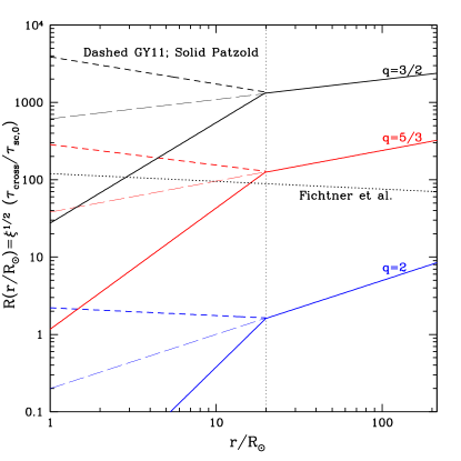
Figure 2: Left: Spatial variation of the ratio $\tau_{\rm cross}\,/\tau_{\rm sc}\,{}_{,0}=R(r/{R_{\odot}},{\gamma}=1)$ (modulo the scaling factor $\xi^{1/2}$) for I-K model with $q=3/2$, Kolmogorov with $q=5/3$, and free transport approximation $q=2$. Note that the ratio $R(r,{\gamma}=1$ is very different for the three models at ${\gamma}=1$ but because of different energy dependence of the models the differences at the relevant energies $10^{4}<{\gamma}<10^{6}$ is much smaller. Right: Radial variations of $A(r/{R_{\odot}},{\gamma})$ defined in Equation (28), for three values of ${\gamma}$ and three values of $q$; $q=3/2,\epsilon=0.25,R_{0}=3000$, $q=5/3,\epsilon=0.40,R_{0}=200$, and $q=2,\epsilon=0,R_{0}=1.0$. As evident the differences between the models at high energies is smaller.

4 CRe Spectral Variation and Resultant Radiation Flux

As described above, CRes with the spectrum observed at 1 AU are guided along $B$ fields following Parker spirals) to the Sun maintaining the isotropic pitch angle distribution because of scattering by turbulence. This process changes (1) their energy loss rate and thus their spectra, and (2) their number density because of the reduction of their bulk flow and focusing by converging magnetic fields.

4.1 Energy Loss Rate and CRe Spectral Variations

The energy loss rate given by Equation (12) is enhanced by the factor $R(r,{\gamma})$. Thus, multiplying the energy loss rate given in Equation (14) by $R({\gamma},r)$ in Equation (23) we obtain

$$d{\gamma}/{\gamma}^{q}=7.8\times 10^{-7}R_{0}g(r/{R_{\odot}})d(r/{R_{\odot}}),\,\,\,\,g(x)=x^{\epsilon}(h(x)+\zeta x^{-2{\delta}})$$ (24)

Integrating this for an electron with initial Lorentz factor ${\gamma}_{0}$ at 1 AU ($x_{au}=214$) gives the variation of Lorentz factor with distance as

$${\gamma}^{(1-q)}(r)={\gamma}_{0}^{(1-q)}+CG(r/{R_{\odot}})\,\,\,\,{\rm with}\,\,\,\,G(x)=\int_{x}^{x_{au}}g(x)dx;\,\,\,C=7.8\times 10^{-7}(q-1)R_{0}.$$ (25)

There is no simple analytic expression for $G(x)$. For this purpose we set $h(x)=0.5(x^{-2}+x^{-n})$, with $n\gg 1$ to account for the sharp increase of $h(x)$ as $x\rightarrow 1$. Using this form, which gives identical value for $G(1)$ for $n=8$, we obtain

$$G(x)=0.5[H_{(1-\epsilon)}+H_{(n-1-\epsilon)}]+\zeta H_{(2{\delta}-1-\epsilon)}\,\,\,{\rm with}\,\,\,H_{a}=(x^{-a}-x_{au}^{-a})/a.$$ (26)

From this we obtain

$${\gamma}_{0}=\left(\frac{{\gamma}}{[1-A(x,{\gamma})]^{1/(q-1)}}\right)\,\,\,\,{\rm and}\,\,\,\,\frac{d{\gamma}_{0}}{d{\gamma}}=\left(\frac{{\gamma}_{0}}{{\gamma}}\right)^{q},$$ (27)

where we have defined the critical function

$$A(x,{\gamma})=CG(x){\gamma}^{(q-1)},$$ (28)

which is shown in Figure 2 (right) for $\xi=0.04$, three values of $q$, and Lorentz factors ${\gamma}=10^{6},10^{5}$ and $10^{4}$. As evident this crucial factor has similar distance dependencies for the three models. However, the dependence on energy (or the Lorentz factor) is more variable.

Given $A(x,{\gamma})$ we obtain the spectral variation with $r$ of CRe density as $N({\gamma},r)=N({\gamma}_{0},r)d{\gamma}_{0}/d{\gamma}=N({\gamma}_{0},r)({\gamma}_{0}/{\gamma})^{q}$. Setting the energy dependence of $N({\gamma}_{0},r)$ to the observed spectrum at 1 AU given in Equation (9), (and changing $E$ to ${\gamma}$) we obtain the spectral shape at different distances inside 1 AU, due to energy loss as

$$N({\gamma},r)=N_{0}(r)\left(\frac{{\gamma}}{[1-A(r/{R_{\odot}})]^{1/(q-1)}}\right)[1-A(r/{R_{\odot}})]^{-q/(q-1)},$$ (29)

where $N_{0}(r)$ describes the spatial variation, with $N_{0}(r=1{\rm AU})=N_{0}$ defined below Equation (9). The (correction) term in the square brackets will be more important at higher energies and closer to the Sun with maximum value at the photosphere with  $G_{\rm max}=G(1)=0.5/(1-\epsilon)+0.5/(n-1-\epsilon)+\zeta/(2{\delta}-1-\epsilon)\sim 1$.

4.2 Spatial Variations

As mentioned above the spatial variation is affected by two processes. First, in the regions where gyro-radius is smaller than $B$ field scale height $H_{B}$ (i.e. $r<r_{\rm cr}$), the convergence of field lines toward the Sun focuses the particles, so that their number density in a bundle of field lines increases inversely with cross sectional area, $A(r)$, of the bundle and $N_{0}(r)\propto 1/A(r)\propto r^{-2}$ for radial or Parker spiral field lines. Second, interactions with turbulence changes the CRe residence time, or the escape time, $T_{\rm esc}\,$. This changes the normalization by the ratio $T_{\rm esc}\,/\tau_{\rm cross}\,$, which in the strong diffusion limit is equal to $\tau_{\rm cross}\,/\tau_{\rm sc}\,{}_{,0}=R_{0}(r)=R_{0}(r/{R_{\odot}})^{\epsilon}$. The combine effect then yields

$$N_{0}(r)=N_{0}(r_{\rm cr})\left(\frac{A(r_{\rm cr})R_{0}(r)}{A(r)R_{0}(r_{\rm cr}))}\right)=N_{0}(r_{\rm cr})(r/r_{\rm cr})^{\epsilon-2}.$$ (30)

As shown in Appendix D, this spatial variation can be derived by integration of Equation (19) over the volume of a bundle of field lines.

4.3 CRe Spectarl Variation

Because of the uncertainty in value of $r_{\rm cr}$, here we focus on effects of commonly ignored energy loss which gives the dependence of flux on energy setting $N_{0}(r)=N_{0}$. Inclusion of the spatial variation in Equation (30) will scale the energy spectra by $(r/r_{\rm cr})^{\epsilon-2}$.

In Figure 3 we show spatial variations of the CRe spectra flux, $F({\gamma},r)=cN({\gamma},r)$, from 1 AU to the photosphere for three models of the transport and two scenarios of the $B$ field structure (Patzold and PSP) described in Equation (4). First we consider the free transport case ignoring scattering and field convergence, which means we set $q=2,R_{0}=1.0$ and $\epsilon=0$. The results are shown on the left panel of Figure 3, which represent the minimum effect of the transport on spectral variation. We also show spectra for two more realistic models of turbulence; The I-K model with $q=3/2,R_{0}=3000,\epsilon=0.25$ in the middle panel, and Kolmogorov with $q=5/3,R_{0}=200,\epsilon=0.40$ in the right panel.

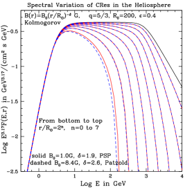
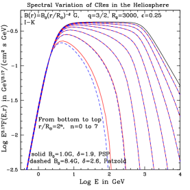
Figure 3: Variation with distance of the spectrum of Cosmic Ray electrons from 1 AU (black line fitted to observed AMS02 and HESS points) to the Sun, at several distances obtained from Equation (29). The top curve shows an analytic fit to the observed data described by Equation (9). The red-solid and blue-dashed curves show spectra for the two specified models of the $B$ field: Left: $q=2,R_{0}=1.0$ and $\epsilon=0.0$, which means we are ignoring scattering and field convergence effects. Middle for Kolmogorov model with $q=5/3,R_{0}=200$ and $\epsilon=0.40$ and right for I-K model with $q=3/2,R_{0}=3000$ and $\epsilon=0.25$; see Figure 2, left.

As evident the most pronounce loss and modification of spectra occurs near the Sun. For a closer comparison of spectra for different turbulence models, on left panel of Figure 4 we show, for two models of the $B$ field, the spectra at the photosphere for the three models of turbulence used in Figure 3. On the right panel, we show spectra for smaller values of the critical parameter, $R_{0}=2000$ and 130 for q=3/2 and 5/3, respectively, to demonstrate the possible range of spectra.

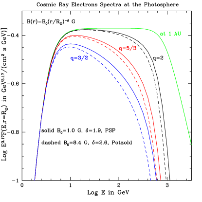
Figure 4: CRe spectra at the photosphere for two $B$ field models (PSP and Patzold). Left, for the three models of turbulence with characteristics given in Figure 3 and right, for different values of the critical parameter $R_{0}=2000,130$ for $q=3/2$ and 5/3, respectively

.

It should be noted that there are some uncertainties in the value of the three primary model parameters, $B_{0},\epsilon$ and $q$, used here, in addition to the uncertainty in the normalization values discussed above (Eq. 30).

Substituting these electron spectra in Equation (1) one can calculate the spectra of synchrotron and IC emissivities, $\eta(\nu,r)$, as a function of distance from the Sun, for appropriate interaction cross sections, which depend directly on the variations with $r$ of the $B$ field and optical photon energy density, respectively.

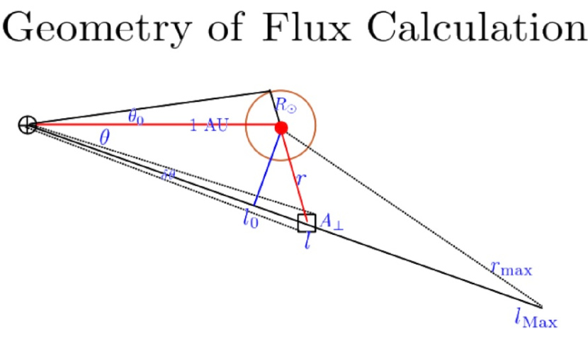
Figure 5: Geometry of calculation of the expected radiative flux at the Earth.

4.4 Expected Radiative Flux at 1 AU

The observed flux of radiation at Earth at the distance 1 AU from the Sun will depend on the angle ${\theta}$ between the observation line of sight and the Sun-Earth connection and angular area $d\Omega=\sin{\theta}d{\theta}d\phi$, depicted in Figure 5. The total flux will be an integral over the line of sight;

$$F(\nu,{\theta}){\delta}\Omega=\int_{0}^{\infty}\frac{\eta(\nu,r)(dV/dl)}{4\pi l^{2}}dl=\frac{d\Omega}{4\pi}\int_{0}^{\infty}\eta(\nu,r)dl,$$ (31)

where the volume element $dV=A_{\perp}dl$ yielding $(dV/dl)/(4\pi l^{2})=(d\Omega/4\pi)$, and $r^{2}=a^{2}+l^{2}-2al\cos{\theta}$, where $a=1$AU. From this we find $dl/dr=\pm r/\sqrt{r^{2}-a^{2}\sin^{2}{\theta}}$, with the minus sign for the integral from the Earth, $l=0$ to $l=l_{0}=a\cos{\theta}$ (or $r=a$ to $r=a\sin{\theta}=l_{0}\tan{\theta}$), and the plus sign for $l=l_{0}$ ($r=a\sin{\theta}$) to, in principal, infinity but in practice we can use $l_{\rm max}=2a\cos{\theta}$ (or $r_{\rm max}=a$) as the upper limit, since most of the radiation will come from the vicinity of the Sun. This makes the two integrals equal yielding

$$F(\nu,{\theta}){\delta}\Omega=\frac{{\delta}\Omega}{2\pi}\int_{a\sin{\theta}}^{a}\eta(\nu,r)\frac{rdr}{\sqrt{r^{2}-a^{2}\sin{\theta}^{2}}}.$$ (32)

Thus, to calculate the expected radiation fluxes from the solar disk and around it we need the electron spectra, $N({\gamma},r)$ from 1 AU to the Sun. For the azimuthally symmetric situation at hand, we integrate over $\phi$ to obtain ${\delta}\Omega=2\pi\sin{\theta}d{\theta}$, and using the dimensionless distances $x=r/{R_{\odot}}$, $x_{au}=a/{R_{\odot}}=214=1/\sin{\theta}_{0}$, we then obtain

$$F(\nu,{\theta}){\delta}\Omega={R_{\odot}}(\sin{\theta}d{\theta})\int_{x_{au}\sin{\theta}}^{x_{au}}\eta(\nu,x=r/{R_{\odot}})\frac{xdx}{\sqrt{x^{2}-x^{2}_{au}\sin^{2}{\theta}}}.$$ (33)

4.4.1 Flux From the Solar Disk and Beyond

For emission at the photosphere (i.e. ${\theta}\leq{\theta}_{0}$), we see only half of the flux because of the high optical depth of the Sun, and the lower limit of the integral, $x_{au}\sin{\theta}=1$ independent of ${\theta}$. Thus, we can change the order of integration, first integrating over the angle ${\theta}$ from 0 to ${\theta}_{0}$ and obtain the flux from the whole disk

$$F_{\rm disc}(\nu)=(1/2){R_{\odot}}\int_{1}^{x_{au}}\eta(\nu,x=r/{R_{\odot}})xdx\int_{0}^{{\theta}_{0}}\frac{\sin{\theta}d{\theta}}{\sqrt{x^{2}-x_{au}^{2}\sin^{2}{\theta}}},$$ (34)

Since ${\theta}_{0}\ll 1$ we can set $\sin{\theta}={\theta}$, in which case the integral over ${\theta}$ can be carried out easily yielding

$$F_{\rm disc}(\nu)=(1/2){R_{\odot}}\sin^{2}{\theta}_{0}\int_{1}^{a/{R_{\odot}}}\eta(\nu,x=r/{R_{\odot}})x(x-\sqrt{x^{2}-1})dx,$$ (35)

with $(1/2){R_{\odot}}\sin^{2}{\theta}_{0}=7.6\times 10^{5}$ cm. At the photosphere the emission increases by a factor of 2. For radiation from regions larger than the Sun, the angle integrated flux can be obtained as:

$$F(\nu,<{\theta})=F_{\rm disc}(\nu)+\int_{{\theta}_{0}}^{\theta}F(\nu,{\theta}^{\prime})\sin^{\prime}{\theta}d{\theta}^{\prime},$$ (36)

where $F(\nu,{\theta}^{\prime})$ is given in Equation (33).

In Summary, given the radiation emissivity $\eta(\nu,r)$ and spectral variation of CRe spectrum, Eq. (29), we can obtain the expected fluxes from the disk, Equation (35), and areas larger than the disk from Equation (36).

5 Summary and Conclusions

CRs are observed in great details by the near Earth instruments around 1 AU and beyond in the outer heliosphere, but there are scant measurements of CRs in the inner heliosphere. However, CRs interacting with solar gas and fields can produce high energy radiation mainly in the gamma-ray range (observed first by EGRET instruments on board CGRO and in greater detail by the Large Area Telescope on board Fermi) involving well known emission processes during the quiet phases of the Sun (QS). Interpretation of these emission processes requires a knowledge of the flux, spectrum and other characteristics of CRs in the inner heliosphere (inside 1 AU), which requires an accurate treatment of the transport of CRs from 1 AU, where these characteristics are known, to the Sun.

The past interpretations of these radiation have treated the transport of CRs using a phenomenological modulation method (see, review by Orlando & Strong (2021)), which has had some success treating transport of CRs from outer boundaries of the solar wind to 1 AU. The primary physical process affecting this transport is the interaction of CRs with turbulence in the solar wind, but in the inner heliosphere other effects such as presence of a strong guiding magnetic field and, for CRes, energy losses become dominant. The modulation methods do not treat these aspects. In particular, to best of our knowledge, the important role of energy losses has not been treated quantitatively.

The aim of this paper is the development of an algorithm for this analysis with focus on the transport of CRes. It is well known that CRes interacting with solar optical photons near the Sun produce some of the observed gamma-rays via the IC process (Abdo et al., 2011). Our results can provide a more accurate treatment of this radiation. On the other hand, there has not been any estimate of possible synchrotron radiation by CRes spiraling along magnetic field lines. Our eventual goal is an accurate calculation of the synchrotron emission using the transport method we have developed in this work. Observation and interpretation of the synchrotron emission by CRes is best carried out during QS when, as we have shown, synchrotron emission near the Sun is expected to be mainly in the extreme ultraviolet (EUV) to hard X-ray (HXR) range. Observation by RHESSI (Hannah et al., 2010) has provided a robust upper limit on the QS flux in the X-ray band from 3 to 100 keV, which can constrain the predictions of the synchrotron model.

Below we give a brief summary of the salient aspects of our paper relevant to the transport of CRe from 1 AU to the Sun.

1. We show that treatment of transport requires kinetic approach because for prevailing $B$ fields, especially closer to the Sun, the gyroradius of ¿ GeV electrons is smaller than the $B$ field scale height so that CRes are tied to the strong guiding field and spiral around them losing significant amount of energy (and producing synchrotron radiation). This transport can be treated by the Fokker-Planck equation including three main ingredients; $B$ field convergence, synchrotron and IC energy losses, and scattering by turbulence. The first two require structure of the amplitude magnetic field and variation of well known photon energy density. The last requires spatial variation of the energy density and spectrum of turbulence.

2. Several instruments, in particular PSP, provide in-situ measures of $B$ field down to about 0.1 AU, and there are several indirect estimates of the $B$ field inside this region. We use a combination of these measurements described in §2.1. For IC energy loss we use solar photon energy variation derived by Orlando & Strong (2008). Several earlier in-situ measurements describe the characteristics of turbulence at around 1 AU and PSP has extended these measures to about 0.1 AU. We have no measurements below this so we rely on extrapolation and some theoretical calculations in this region.

3. Instead of solving the kinetic equation numerically we use a simpler method based on numerical simulations by Effenberger & Petrosian (2018), which accounts for field convergence and pitch angel diffusion, $D_{\mu\mu}$, due to scattering with turbulence. This method introduces the concept of resident time or escape time, which allows to separate determination of the spatial and spectral variations. In addition, the ratio of the escape to free crossing time enhances the rates of synchrotron and IC energy losses, and reduces the overall density of the CRes. The density, however, increase toward the Sun, in regions where gyro radius is small, due to focusing effect of the converging field lines. This critical time scale, described in Equation (20), depends on the free advection or crossing time, $\tau_{\rm cross}\,$, on $B$ field scale height, $H_{B}$, and the mean free path, $\lambda_{\rm mfp}$, or scattering time, $\tau_{\rm sc}\,=\lambda_{\rm mfp}/v\sim\langle 1/D_{\mu\mu}\rangle$, which is the most critical scale.

4. In general, the mean free path or scattering time depend on characteristics of turbulence, plus $B$ field and plasma density, in a complicated way. However, for relativistic electrons, which interact mainly with low frequency Alfvén or fast mode turbulence, this relation is considerably simplified and depends on two parameters; the Alfvén speed and a interaction rate (or time scale) that bundles several turbulence and $B$ field parameters into one, described by Equation (22), which varies with distance in a complicated way. The detailed descriptions of variation with distance of turbulence characteristics and calculation of this critical time scale are given in Appendices A and B. These results are summarized in Figures 2 (left) and 6. The energy dependence in the relativistic regime is simple with $\tau_{\rm sc}\,\propto{\gamma}^{2-q}$, where $q$ is the power law index of turbulence in the inertial range, and according to PSP measurement it varies from Kolmogorov (outer region) value of 5/3 to I-K value of 3/2, from about 0.3 to 0.2 AU.

5. We use both of the above models and a third with $q=2$ to account for free (unaffected by $B$ field and turbulence) transport case, which shows the effects of energy loss alone, and calculate the spectral and spatial variation with distance of the CRe spectrum and density (or flux) from their measured values at 1 AU to the Sun. The spatial variation derivation is detailed in Appendix D.

6. These spectra can be used to calculate the emissivity of synchrotron and IC emissions, as described in §2, and the expected radiation flux at 1 AU from the disk of the Sun and regions around it, described in §4.4.

In forthcoming papers, using these models of transport and resultant CRe spectra, we will calculate the IC spectra more accurately than done previously, and the synchrotron spectra for the first time. These can then be compared with observations by Fermi-LAT and RHESSI.

The work of VP is supported by NASA Living With Star program grant NNH20ZDA001N-LWS. E.O. acknowledges the ASI-INAF agreement n. 2017-14-H.0, the NASA Grant No. 80NSSC20K1558.

6 Appendix A: In Situ Measurements of Turbulence

In this section we summarize three in situ measurements of intensity and spectrum of turbulence in the frequency range of $10^{-5}<f<1$ Hz, with corresponding wave numbers $k=2\pi f/v_{A}$. Most of these show a Kolmogorov spectrum, with power-law index $q=5/3$ in the inertial range ($f_{\rm min}<f<f_{\rm max}$). There is generally some steepening above, and most measurements show a distinct spectral flattening below this range with index $q\sim 1$ down to measured limit of $f_{\rm lim}\sim 10^{-5}$ Hz. We need to calculate the total energy density of turbulence ${\cal W}_{\rm turb}=\int_{f_{\rm lim}}^{f_{1}}{\cal W}(f)df$. Assuming that to spectrum below $f_{\rm min}$ extends to $f_{\rm lim}$ with index $q=1$, it is easy to show that

$${\cal W}_{\rm turb}=f_{\rm min}{\cal W}(f_{\rm min})\frac{1}{q-1}\left[1-(f_{\rm min}/f_{\rm max})^{(q-1)}+\ln(f_{\rm min}/f_{\rm lim})\right].$$ (37)

Leamon et al. (1998. 1999) measure a Kolmogorov spectrum ($q=5/3)$ at $\sim 1$ AU with the specific energy density of ${\cal W}(f_{\rm min})=10^{3}$ (nT)² Hz ^-1, in the inertial range $f_{\rm min}=10^{-3},f_{\rm max}=0.1$ Hz. The spectrum steepens to $q\sim 3$ above 0.1 Hz. This yields a total turbulence energy density of ${\cal W}(f>f_{\rm min})\sim 1.5$(nT)². They do not provide any measurements below $f_{\rm min}$, but extending this to $f_{\rm lim}=10^{-5}$ yields ${\cal W}_{\rm turb}\sim 7$ (nT)².

Bruno and Carbone (2013) show the Helios measurements at $r=0.9,0.7$ and 0.3 AU, with Kolmogorov spectrum between $f=0.1$ and $f_{\rm min}$, which decreases slightly with distance. Below $f_{\rm min}$ the spectrum flattens to $q\sim 1$ down to $f_{\rm lim}=2\times 10^{-5}$ Hz. From these we obtain

$${\cal W}(f>f_{\rm min})=\begin{cases}5.0\,\,{\rm nT}^{2}&f_{\rm min}=6\times 10^{-4}\,{\rm Hz},\,r=0.9{\rm AU}\\ 15.0\,\,{\rm nT}^{2}&f_{\rm min}=2\times 10^{-3}\,{\rm Hz},\,r=0.7{\rm AU}\\ 156\,\,{\rm nT}^{2}&f_{\rm min}=5\times 10^{-3}\,{\rm Hz},\,r=0.3{\rm AU}.\end{cases}$$ (38)

Extending to $f_{\rm lim}=10^{-5}$ Hz, we obtain the total turbulence energy densities of

$${\cal W}_{\rm turb}(r)=\begin{cases}20\,\,{\rm nT}^{2}&\,r=0.9{\rm AU},\\ 61\,\,{\rm nT}^{2}&\,r=0.7{\rm AU},\\ 620\,\,{\rm nT}^{2}&\,r=0.3{\rm AU}.\end{cases}$$ (39)

Recently, PSP measurements (Chen et al. 2020) have extended this information from 1 to 0.17 AU, and in the spectral range $2\times 10^{-5}<f<1$ Hz, showing a gradual change of the spectral index $q$ above $f_{\rm min}=10^{-3}$, from Kolmogorov 5/3 value at $r>0.3$ AU to Iroshnikov-Kraichnin (I-K) value of 1.5 for $r<0.2$ AU. In a similar manner as above, estimation based on Figure 1 of Chen et al. (2020), gives the following values for turbulence energy density.

$${\cal W}_{\rm turb}(r)=\begin{cases}10\,\,{\rm nT}^{2}&f_{\rm min}=10^{-4}\,{\rm Hz},\,\,\,\,\,\,\,\,\,\,\,r=0.82{\rm AU},\\ 83\,\,{\rm nT}^{2}&f_{\rm min}=2\times 10^{-4}\,{\rm Hz},\,\,r=0.5{\rm AU},\\ 730\,\,{\rm nT}^{2}&f_{\rm min}=5\times 10^{-4}\,{\rm Hz},\,\,r=0.3{\rm AU},\\ 4800\,\,{\rm nT}^{2}&f_{\rm min}=10^{-3}\,{\rm Hz},\,\,\,\,\,\,\,\,\,\,\,r=0.17{\rm AU}.\end{cases}$$ (40)

The break frequency, $f_{\rm min}$, seem to increase inversely with distance as, $f_{\rm min}\sim 10^{-4}(AU/r)$  Hz, with PSP showing slightly smaller values than Helios. The values of ${\cal W}_{\rm turb}(r)$ are plotted in Figure 6 showing rough agreement between different estimates. A power-law fit to these 8 measured values yields

$${\cal W}_{\rm turb}(r)=12(r/{\rm AU})^{-3.1}\,{\rm nT}^{2}=0.033(r/{R_{\odot}})^{-3.1}{\rm G}^{2},\,\,\,0.1<(r/{\rm AU})<1.$$ (41)

We will use this relation below.

We have no information on turbulence energy density in the more critical inner region ($r<20{R_{\odot}}$). We consider two methods of extrapolation to the inner region. In one we assume that the above radial dependence continues to the Sun, then using the $B(r)$ field models described in §2 we calculate the ratio of turbulence to magnetic field energy densities, $f_{\rm turb}(r)={\cal W}_{\rm turb}(r)/[B(r)]^{2}$, needed for evaluation of $\tau_{\rm sc}\,$ and ELEF (see below), to be

$$f_{\rm turb}(r)=\begin{cases}0.033(r/{R_{\odot}})^{0.6}&\,20<r/{R_{\odot}}<214\\ 0.35(r/{R_{\odot}})^{-0.2}&\,r/{R_{\odot}}<20,\,\,\,{\rm GY11}\\ 4.7\times 10^{-4}(r/{R_{\odot}})^{2.0}&\,r/{R_{\odot}}<20,\,\,\,{\rm Patzold}.\end{cases}$$ (42)

However, considering that the turbulence energy density is almost proportional to $[B(r)]^{2}$ in the outer region, it is reasonable to assume that, like the $B$ field in Patzold model, ${\cal W}_{\rm turb}(r)$ increases faster in the inner region yielding a flatter, nearly constant $f_{\rm turb}(r)\sim 0.3$. We will use a combination of both these extrapolations shown in Figure 2.

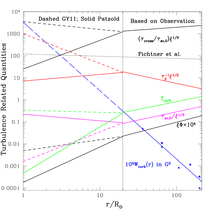
Figure 6: Radial variations of CRe energy independent relevant quantities related to turbulence and scattering of the particles assuming the I-K model with $q=3/2$. $\Phi(x)$, Eq. (47), (solid-black); turbulence energy density $W_{\rm turb}$, Eq. (41), in blue; turbulence to $B$ field energy ratio, $f_{\rm turb}$, Eq. (42), in green; characteristic turbulence rate $\tau_{p}^{-1}$, Eq. (44), in red; scattering time $\tau_{\rm sc}\,{}_{,0}$, Eq. (45), in magenta; and the crossing to scattering time ratio, Eq. (50), in black. The results in the outer region are based on PSP measurements, with extrapolation to the inner part (long dashed). The two dashed and solid lines in the inner part are based on the two models of the $B$ field models, GY11 and Patzold. The dotted line is based on theoretical results from Fichtner et al. (2012).

7 Appendix B: Scattering Time

The pitch angle diffusion coefficient, $D_{\mu\mu}$, and hence $\kappa_{ss}$ and $\tau_{\rm sc}\,$, can be obtained from gyro-resonance interaction rates of particles with plasma waves of frequency $\omega$ and wave vector $k$, obeying the resonance condition

$$\omega(k)-k_{\|}\mu v=\pm\Omega/{\gamma},$$ (43)

where $v$, ${\gamma}$ and $\Omega$ are the velocity, Lorentz factor and gyrofrequency of the the particle, and $k_{\|}$ is the component of the wave vector parallel to the $B$ field. The interaction rates depend on the dispersion relation of the waves, $\omega(k)$, the energy density of the waves, ${\cal W}_{\rm turb}$, its spectrum (mainly the spectral index $q$ in the inertial range; $k_{\rm min}<k<k_{\rm max}$), and the background plasma $B$ field and density, $n$ (or Alfvén velocity, $v_{A}$). However, for a power-law spectrum of turbulence, ${\cal W}(k)={\cal W}(k_{\rm min})(k/k_{\rm min})^{-q}$, the diffusion rate (or scattering time) scales with the characteristic time $\tau_{p}$ or characteristic rate (see, e.g. Dung & Petrosian 1994)

$$\tau_{p}^{-1}=(\pi/2)\Omega f_{\rm turb}(q-1)\Phi^{(q-1)}\,\,\,\,{\rm with}\,\,\,\,\Phi=ck_{\rm min}/\Omega,$$ (44)

where fraction of turbulence energy density, $f_{\rm turb}\sim(\delta B/B)^{2}$ is given in Appendix A.

In general, the scattering time, in addition to this scaling, depends in a complicated way on $q$ and Alfvén velocity (or $\beta_{A}=v_{A}/c$), and on particle energy and pitch angle (see, e.g. Pryadko & Petrosian 1997, 1999, Petrosian & Liu 2004 Jiang et al. 2009). However, for high energy protons and relativistic electrons with Lorentz factors ${\gamma}>m_{p}/m_{e}$, i.e. energies greater than 1 GeV, which is the case for our problem, the main interactions are with Alfv́en waves, with the dispersion relation $\omega=k_{\|}v_{A}$ for waves propagating parallel to the $B$ field and for $\omega<\Omega_{p}$, the proton gyrofrequency, and with fast mode waves with $\omega=kv_{A}$ and $k\ll 1$ for both parallel and perpendicular wave propagation. In this case the equations describing the above characteristics are simplified considerably, especially when ${\beta}_{A}\ll 1$, which is the case here. As shown in Figure 1, $v_{A}$ has nearly a constant value of $\sim 500$ km/s in the inner region ($r<20{R_{\odot}}$) and decreases with distance to 30 km/s at 1 AU as $v_{A}=30(AU/r)^{1.2}$.

As shown in Pryadko & Petrosian (1997) and Petrosian & Liu (2004) for parallel propagating waves, the pitch angle averaged scattering time appropriate for relativistic electrons with isotropic pitch angle distributions, and for $\beta_{A}\ll 1$, is

$$\tau_{\rm sc}\,={\gamma}^{(2-q)}\tau_{\rm sc}\,{}_{,0}\,\,\,{\rm with}\,\,\,\tau_{\rm sc}\,{}_{,0}/\tau_{p}=\begin{cases}2[(2-q)(4-q)]^{-1}&\,q<2\\ 3/4-(1/2)\ln\beta_{A}&\,q=2.\end{cases}$$ (45)

Using $v_{A}=500$ km/s for $r<20{R_{\odot}}$, where most of the losses take place, we obtain

$$\tau_{\rm sc}\,{}_{/}\tau_{p}=\begin{cases}1.6{\gamma}^{(1/2)}&\,q=3/2\\ 2.6{\gamma}^{(1/3)}&\,q=5/3\\ 3.9&\,q=2.\end{cases}$$ (46)

7.1 Scaling Details

To complete the calculation of the scattering time we need to specify the numerical value of $\tau_{p}$ and its variation with distance, which depends on $\Omega_{e}$ (or $B$ field), $f_{\rm turb}$, and the somewhat unknown $k_{\rm min}=2\pi f_{\rm min}/v_{A}$, the inverse of the largest scale of the turbulence. This length scale is related to the correlation length of the injected turbulence and is expected to be a fraction, $\xi$, of the size of the region, here $\sim r$, defined as $\xi=2\pi/(k_{\rm min}r)$. The correlation length at the base of the corona, $r={R_{\odot}}$, is estimated to be $2\pi/k_{\rm min}\sim 10^{9}$ cm implying $\xi\sim 0.03$. The correlation length most probably increases with distance. PSP observations of decreasing $f_{\rm min}\sim 10^{-4}(AU/r)$ in the outer regions seem to agree with this. Using $f_{\rm min}\sim 2\times 10^{-3}$ and $v_{A}=500$  km/s at $r=20{R_{\odot}}$ yields $\xi\sim 0.04$. For now we will keep $\xi$ as a free parameter.

Using the general magnetic field model of $B(r)=B_{0}x^{-{\delta}}$, with $x=r/{R_{\odot}}$ we obtain

$$\Phi\frac{ck_{\rm min}}{\Omega_{e}}=\Phi_{0}\frac{x^{{\delta}-1}}{B_{0}}=\Phi_{0}\begin{cases}1.0x^{0.9}&\,20<x<214\\ 3.3x^{0.5}&\,1<x<20\,\,\,{\rm BY11}\\ 0.12x^{1.6}&\,1<x<20\,\,\,{\rm Patzold},\end{cases}$$ (47)

with $\Phi_{0}=1.5\times 10^{-7}/\xi\sim 3.7\times 10^{-6}$. PSP observations indicate that the spectral index changes from 5/3 to 3/2 between 0.3 and 0.2 AU. We are not aware of any direct measurement of the index closer to the Sun where the energy loss rate is most significant. Thus, we will consider three values of $q=3/2,5/3$ and 2. Now substituting the above values for $\Phi,q,f_{\rm turb}$ and the magnetic field, in Equations (44) and (45) we can calculate $\tau_{p}^{-1}$ and $\tau_{\rm sc}\,$. For example, for $q=3/2$ we obtain

$$\tau_{p}^{-1}=(0.04/\xi)^{1/2}\begin{cases}1.4\times 10^{2}(r/{R_{\odot}})^{-0.70}&\,20<x<214\\ 4.8\times 10^{3}(r/{R_{\odot}})^{-1.25}&\,x<20,\,\,\,{\rm GY11}\\ 76(r/{R_{\odot}})^{0.2}&\,x<20,\,\,\,{\rm Patzold},\end{cases}$$ (48)

and from Equation (45) we obtain

$$\tau_{\rm sc}\,{}_{,0}=(\xi/0.04)^{1/2}\begin{cases}1.8\times 10^{-2}(r/{R_{\odot}})^{0.75}&\,20<r/{R_{\odot}}<214\\ 3.4\times 10^{-4}(r/{R_{\odot}})^{1.35}&\,r/{R_{\odot}}<20,\,\,\,{\rm GY11}\\ 2.1\times 10^{-2}(r/{R_{\odot}})^{-0.3}&\,r/{R_{\odot}}<20,\,\,\,{\rm Patzold},\end{cases}$$ (49)

which for $\tau_{\rm cross}\,=5.6x$ (Eq. 15) gives the critical ratio (for $q=3/2$)

$$\tau_{\rm cross}\,/\tau_{\rm sc}\,{}_{,0}=(0.04/\xi)^{1/2}\begin{cases}1.6\times 10^{2}(r/{R_{\odot}})^{0.25}&\,20<r/{R_{\odot}}<214\\ 8.2\times 10^{3}(r/{R_{\odot}})^{-0.35}&\,r/{R_{\odot}}<20,\,\,\,{\rm GY11}\\ 1.3\times 10^{2}(r/{R_{\odot}})^{1.3}&\,r/{R_{\odot}}<20,\,\,\,{\rm Patzold}.\end{cases}$$ (50)

Similar expressions can be obtained for the other two values of $q$. Left panel of Figure 2 shows $\tau_{\rm cross}\,/\tau_{\rm sc}\,{}_{,0}$ for the three values of $q$. As evident there is a large difference between the two models of the $B$ field in the inner region. This is due to the extrapolation of ${\cal W}_{\rm turb}$ from outer to inner region, which as mentioned in Appendix A may not be correct. Using the flatter variation of $f_{\rm turb}$ in the inner region we obtain the dashed lines which are half way between the two models of $B(r)$. We will use these extrapolations, which give the ratio $\tau_{\rm cross}\,/\tau_{\rm sc}\,$ at ${\gamma}=1$.

The final crucial ratio $R(r,{\gamma})$ can then be obtained using Equation (20). However, as evident $\tau_{\rm sc}\,<\tau_{\rm cross}\,$, even at the highest energies, ${\gamma}<10^{6}$, especially for $q=3/2$ and 5/3, implying that we are in the strong diffusion limit with $R(r,{\gamma})=[\tau_{\rm cross}\,(r)/\tau_{\rm sc}\,{}_{,0}(r)]{\gamma}^{(q-2)}$.

There have been many theoretical attempts to estimate the radial and energy dependence of the above characteristics of turbulence in the heliosphere, in particular that of the scattering time or mean free path $\lambda_{\rm mfp}(r,{\gamma})=\lambda_{0}(r/AU)^{{\delta}_{l}}{\gamma}^{(2-q)}$. For example, Chhiber et al. (2017) present several results from MHD simulations on the spatial variation (for $r<1$ AU) of the mean free path of protons with $0<{\delta}_{l}<0.6$, and $\lambda_{0}\sim 0.2\pm 0.1$ AU or $\tau_{\rm sc}\,{}_{,0}\sim 100$ s at 1 AU, which is much larger than $\tau_{\rm sc}\,{}_{,0}$ obtained from observations shown above. Fichtner et al. (2012) give result for scattering of 10 MeV protons by Alfv́en waves showing $\lambda_{\rm mfp}/r$ varying from 0.02 at the Sun to 0.01 at 1 AU. Based on results from Petrosian & Liu (2004) this indicates a $\lambda_{\rm mfp}/r=0.02{\gamma}^{(2-q)}$ for relativistic electrons, or $\tau_{\rm sc}\,{}_{,0}\sim 0.047$ s at $r={R_{\odot}}$.

The ratio $\tau_{\rm cross}\,/\tau_{\rm sc}\,{}_{,0}$ for the Fichtner model is also shown on the left panel of Figure 2, which lies between $q=3/2$ and 5/3 cases. The actual effect of the transport coefficients is better demonstrated by the term $A(x,{\gamma})$ defined in Equation (28) shown in Figure 2 (right) for the three values of $q$ and Lorentz factors ${\gamma}=10^{6},10^{5}$ and $10^{4}$.

As evident the spatial variation of this crucial factor is similar for the three values of the index $q$, but there is significant differences in their energy dependencies. However, these differences are much smaller For $10^{3}<{\gamma}<10^{6}$ compared to the values shown for ${\gamma}=1$ (left panel).

8 APPENDIX C: Perpendicular Diffusion

In strong guiding $B$ fields diffusion perpendicular to the field lines can be ignored, but when scattering mean free path becomes comparable to or larger than the particle gyro-radius, perpendicular diffusion becomes important. As shown in §3.1 the gyro-radius of relativistic electrons is $r_{g}=1.3\times 10^{3}{\gamma}({\rm G}/B)$ cm and the mean free path $\lambda_{\rm mfp}=c\tau_{\rm sc}\,=ca(q){\gamma}^{(2-q)}\tau_{p}$, where $a(q)$ and $\tau_{p}$ are given in Appendix B. Simple algebra shows that

$$R_{\rm diff}\equiv r_{g}/\lambda_{\rm mfp}=\pi/[4a(q)]f_{\rm turb}({\gamma}\Phi)^{(q-1)}.$$ (51)

In the outer region ($r>20{R_{\odot}}$) with $q=5/3,a(q)=2.6,\Phi=\Phi_{0}x^{0.9}$ and $f_{\rm turb}=0.033x^{0.6}$ we obtain

$$R_{\rm diff}=1.3\times 10^{-7}{\gamma}^{2/3}x^{1.2}$$ (52)

so that for ${\gamma}\leq 10^{6}$ $R_{\rm diff}\leq 0.8$ and 0.05 for at 1 AU and $r=20{R_{\odot}}$, respectively. In the inner region ($r<20{R_{\odot}}$) with $q=3/2,a(q)=1.6,\Phi=1.2\Phi_{0}x^{1.6}$ and $f_{\rm turb}=4.7\times x^{2.0}$ we obtain

$$R_{\rm diff}=5\times 10^{-7}{\gamma}^{1/2}x^{2.6}$$ (53)

so that for ${\gamma}\leq 10^{6}$, $R_{\rm diff}\leq 10^{-4}$ and 0.05 at the Sun and $r=20{R_{\odot}}$, respectively.

Because we are mainly interested in the inner region the neglect of perpendicular diffusion is well justified.

9 APPENDIX D: Details of Density Variation

Here we use the steady state, $\partial N/\partial t=0$, Equation (19). We first note that for relativistic CRes, $\kappa_{ss}=3v^{2}\tau_{\rm sc}\,=3c^{2}\tau_{\rm sc}\,{}_{,0}{\gamma}^{(2-q)}$, so that if we multiply this equation by $q^{(q-2)}$, the first term in this equation will depend only on the spatial variable and describes the implicit spatial variation $N_{0}(r)$. This also will alter the energy loss rate by this factor similar to what was used in §4.1. If we now ignore the energy terms, we can obtain a simple approximate solution for the CRe density variation by integration of the resultant equation over the volume, $dV(s)=A_{\perp}(s)ds$, of a bundle of field lines with cross section area, $A_{\perp}(s)$, from the starting point $s=0$, the point where kinetic equation becomes valid ($r=r_{\rm cr}\sim 10{R_{\odot}}$), to any $s$ (or any $r<r_{\rm cr}$). We set $ds=1.2dr,\tau_{\rm cross}\,=1.2r/c$ and $R_{0}(r)=\tau_{\rm cross}\,/\tau_{\rm sc}\,{}_{,0}=R_{0}(r/{R_{\odot}})^{\epsilon}$ to obtain $N(r)$ by integration over $s$ as:

$${\gamma}^{(q-2)}\int_{0}^{s}A_{\perp}(s)\frac{\partial}{\partial s}\kappa_{ss}\frac{\partial N}{\partial s}ds=\frac{3c^{2}}{1.2}\left(\tau_{\rm sc}\,{}_{,0}A\frac{dN}{dr}\right)_{r_{\rm c}}^{r}-\frac{3c^{2}}{1.2}\int_{r_{\rm cr}}^{r}N(r)\frac{d(\tau_{\rm sc}\,{}_{,0}A)}{dr}=0.$$ (54)

Since $A(r)\propto r^{2}$ and $\tau_{\rm sc}\,{}_{0}(r)\propto r^{{\delta}_{sc}}$ obey simple power laws we expect a power law behavior for $N(r)$ and can set $dN/dr=(N/r)(d\ln N/d\ln r)$, with the power law index ${\delta}_{N}=d\ln N/d\ln r$ nearly a constant. This then allows to complete the integration, which after some algebra leads to

$$N(r)=N(r_{\rm cr})\left(\frac{A(r_{\rm cr})R_{0}(r)}{A(r)R_{0}(r_{\rm cr}))}\right),$$ (55)

which leads to the conjecture in Equation (29).

References

- Abdo et al. (2011) Abdo, A. A., Ackerman, M. Ajello, M., et al. 2011, ApJ, 734, 116
- Aguilar et al. (2014) Aguilar, M., Aisa, D., Alvino, A., et al., 2014 Phys. Rev. Letters, 113, 121102
- Alissandrakis & Gary (2021) Alissandrakis, C. E., & Gary, D. E., 2021, Front. Asron. and Space Sci., 7, 77A
- Badman et al. (2021) Badman, S. T., Bale, S. D., Rouillard, A. P., et al., 2021, Astronomy & Astrophysics, 650, 26
- Bruno & Carbone (2005) Bruno, R. & Carbone, V., 2013, Living Review of Solar Physics, 10, 2
- Chen et al. (2020) Chen, C. H. K., Bale, S. D., Bonnel, J. W., et al., 2020, ApJ Suppliment Series, 240, 53
- Chhiber et al. (2017) Chhiber, R., Subedi, P., Usmanov, A. V., et al., 2017, ApJ Suppliment Series, 230, 21
- Dung & Petrosian (1994) Dung, R., & Petrosian, V., 1994, ApJ, 421, 550
- Effenberger & Petrosian (2018) Effenberger, F., & Petrosian, V., 2018, ApJ, 868, L28
- Fujii & McDonald (2005) Fujii, Z., & McDonald, F. B., 2005, Adv. in Sp Research, 35, 611
- Fichtner, et al. (2002) Fichtner et al., 2002, Astrtoparticle Physics, 17, 199
- Gopalswamy & Yashiro (2011) Gopalswamy, Nat & Yashiro, Seiji, 2011, ApJ, 736, L17
- Hannah et al. (2010) Hannah, I. G., Hudson H. S., Hurford, G. J., & Lin, R. P., 2010, ApJ, 724, 487
- HESS Collaboration (2017) H.E.S.S. Collaboration; Kerszberg, D., et al., 2017, Presented at the ICRC, Buson, Korea 640, L155 (2006), arXiv:astro-ph/0511149 [astro-ph].
- Hooper et al. (2017) Hooper, D., Cholis, I., Linden T., & Fang, K., 2017, Phys. Rev. D 96, 103013.
- Jiang et al. (2009) Jiang Y., Liu, S., & Petrosian, V., 2009, ApJ, 698, 163
- Leamon et al. (1998) Leamon, R. J., Smith, C. W., & Ness, N. F., 1998, J. Geophys. Res., 103, 4775
- Leamon et al. (1999) Leamon, R. J., Smith, C. W., Ness, N. F., 1999, J. Geophys. Res., 104, 22331
- Lehblanc et al. (1998) Lehblanc, Y., Dulk, G. A., Bougeret, J.-L., 1998, Sol. Phys., 183, 165
- Malyshkin $ Kulsrud (2001) Malyshkin, L., & Kulsrud, R., 2011, ApJ, 549, 402
- Moderski et al. (2005) Moderski, R., Sikora, M., Coppi, P. S., & Aharonian, F. 2005, MNRAS, 363, 954
- Moskalenko, et al. (2006) Moskalenko, I. V., Porter, T. A., & Digel, S. W., 2006, ApJ, 652, L65
- Orlando & Strong (2007) Orlando, E. & Strong, A. W. 2007, Ap&SS, 309, 359. doi:10.1007/s10509-007-9457-0
- Orlando & Strong (2008) Orlando, E., & Strong, A. W., 2008, A&A, 480, 847
- Orlando & Strong (2021) Orlando, E., & Strong, A. W., 2021, Journal of Cosmology and Astroparticle Physics, 04, 004
- Orlando (2008) Orlando, E. 2008, PhD Thesis, https://ui.adsabs.harvard.edu/abs/2008PhDThesis
- Petrosian (2012) Petrosian, V., 1985, ApJ, 299, 987 (Eq. A4)
- Petrosian (2012) Petrosian, V., 2012, Space Sci Rev., 173, 535
- Petrosian & Liu. (2004) Petrosian, V., & Liu, S., 2004, ApJ, 610, 550
- Patzold et al. (1987) Patzold, M., Bird, M. K., Levy, G. S., et al., 1987, Sol. Phys., 109, 91
- Pryadko & Petrosian (1997) Pryadko, J. M., & Petrosian, V., 1997, ApJ, 482, 774
- Pryadko & Petrosian (1999) Pryadko, J. M., & Petrosian, V., 1999, ApJ, 515, 873
- Rybicki & Lightman (1980) Rybicki, G. B. & Lightman, A. P., 1980 Radiation Processes in Astrophysics, J. Willy & Sons, New York
- Saito et al. (1997) Saito, K., Poland, A. I., Munro, R. H., 1977, Sol. Phys., 55, 121