Margin-based sampling in high dimensions:
When being active is less efficient than staying passive

Abstract

It is widely believed that given the same labeling budget, active learning (AL) algorithms like margin-based active learning achieve better predictive performance than passive learning (PL), albeit at a higher computational cost. Recent empirical evidence suggests that this added cost might be in vain, as margin-based AL can sometimes perform even worse than PL. While existing works offer different explanations in the low-dimensional regime, this paper shows that the underlying mechanism is entirely different in high dimensions: we prove for logistic regression that PL outperforms margin-based AL even for noiseless data and when using the Bayes optimal decision boundary for sampling. Insights from our proof indicate that this high-dimensional phenomenon is exacerbated when the separation between the classes is small. We corroborate this intuition with experiments on 20 high-dimensional datasets spanning a diverse range of applications, from finance and histology to chemistry and computer vision.

1 Introduction

In numerous machine learning applications, it is often prohibitively expensive to acquire labeled data, even when unlabeled data is readily available. For instance, consider the task of inferring the sleep quality of a patient from data collected during usual health checks (e.g. EEG, EKG, blood tests etc). To get a high-precision label for this task, patients need to spend a night in a sleep lab, which is expensive and time-consuming. Therefore, the labeled dataset that we can collect cannot be too large. However, a large unlabeled set of medical records of similar patients is available and can potentially be leveraged for the task. Active learning algorithms aim to reduce labeling costs, by collecting a small labeled set that still results in a model with good predictive performance.

A popular family of active learning algorithms is margin-based active learning (M-AL) [33, 1, 10]. This paradigm proposes to alternate between (i) training a prediction model (e.g. logistic regression, deep neural network) on the currently available labeled set; and (ii) augmenting the labeled set by acquiring labels for the unlabeled points that lie close to the decision boundary of the model. M-AL is closely related to strategies like uncertainty sampling [24], entropy sampling [38], or softmax sampling for neural networks.

Numerous prior works have documented the success of M-AL in low dimensions [42, 34, 47, 35]. As it is evident in Figure 1, in the regime where the query budget is large (i.e. $n_{\ell}\gg d$), M-AL achieves low test error with a lot less labeled data than passive learning (PL, i.e. uniform sampling). This is in line with the intuition about M-AL developed in prior works. At the same time, the figure reveals that in the low-sample regime (i.e. $n_{\ell}\ll d$) M-AL “fails” – that is, it leads to worse predictive error than PL. This regime is much less studied in the AL literature.

In this paper, we characterize theoretically and empirically the settings that lead to the failure of M-AL for high-dimensional logistic regression. We rule out two likely causes for this phenomenon. First, it is known that, in low dimensions, M-AL does not improve upon the sample efficiency of PL when the Bayes optimal model has high error [28]. Second, several works [20, 37, 16] argue that M-AL can fail due to the cold start problem: using only a small labeled set, one cannot obtain a meaningful decision boundary to be used for sampling.

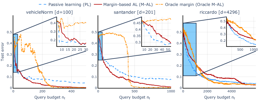
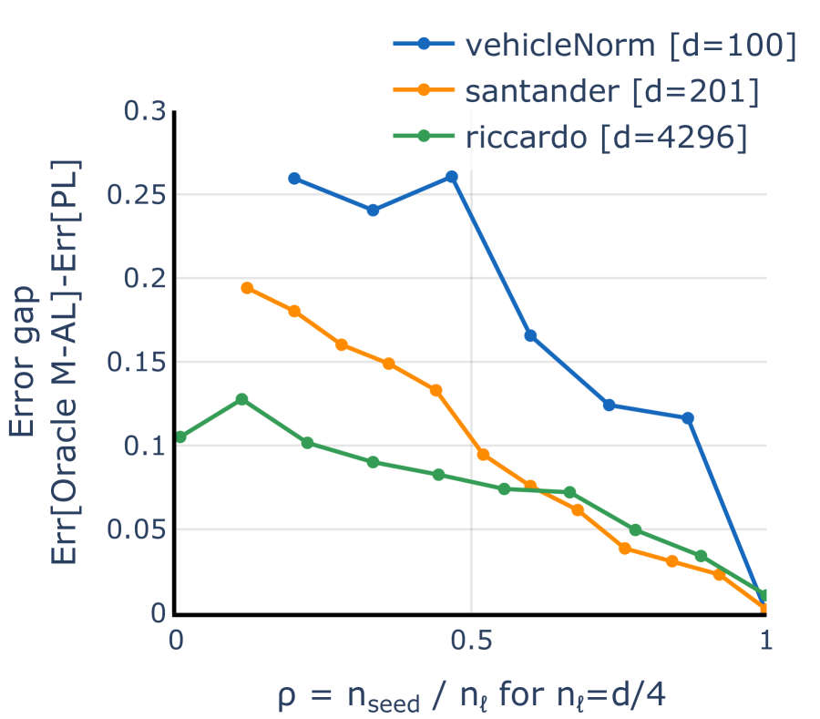
Figure 1: Left: In the low-dimensional regime ($n_{\ell}\gg d$) M-AL achieves low test error with fewer labeled samples than PL. However, in the high-dimensional regime ($n_{\ell}\ll d$, see zoomed-in insets), M-AL fails. Oracle M-AL exhibits the same failure in high dimensions, despite performing well for large query budgets, thus ruling out the cold start problem as a cause for this phenomenon. Right: Increasing the seed set size $n_{\text{seed}}$ reduces the gap between Oracle M-AL and PL. See Appendix G.3 for more datasets.

Perhaps surprisingly, for high-dimensional problems with a low labeling budget, M-AL underperforms PL even when (i) the Bayes error is zero; and (ii) one uses the distance to the Bayes optimal decision boundary for sampling (referred to as oracle margin-based active learning or Oracle M-AL). Our experiments reveal the failure of M-AL for logistic regression on a wide variety of datasets, a subset of which are presented in Figure 1 (a few works make a similar observation for neural networks [37, 16, 40]). This failure of M-AL occurs only in the low-budget regime (see zoomed-in insets in Figure 1), which coincides with the scenario in which AL is often employed in practice (i.e. high labeling costs). Since prior explanations do not apply to the setting that we consider (high-dimensional, noiseless), to date, there exists no result that sheds light on this failure case. Our contributions in this paper are as follows:

1. We observe that M-AL performs worse than PL for logistic regression on numerous high-dimensional datasets from different application domains (e.g. finance, chemistry, histology).

2. We prove non-asymptotic error bounds for logistic regression that directly imply worse performance of M-AL compared to PL – even when using Oracle M-AL (Section 3) and for data distributions with noiseless labels (truncated Gaussian mixture and Gaussian marginal).

3. Distinct from the low-dimensional intuition [28], our proof suggests that in high dimensions M-AL benefits from a large separation margin between the classes. We confirm this intuition experimentally for logistic regression on $15$ real-world datasets (Section 4).

Our results reveal that for high-dimensional data, margin-based AL is not only more computationally costly compared to passive learning, but often provably less effective as well. Our paper hence suggests an important avenue for future work: identify active learning algorithms that are provably consistent and substantially outperform passive learning in high-dimensional and low-budget settings.

2 Active learning for classification

We now introduce the active learning framework that we consider throughout this paper. Our high-level goal is to train a binary classifier that predicts a label $y\in\{-1,1\}$ from covariates $x\in\mathbb{R}^{d}$, where $(x,y)\sim\mathbb{P}_{XY}$. More specifically, we seek parameters $\theta\in\Theta$ such that the classifier $x\rightarrow\operatorname{sgn}\left(f(x;\theta)\right)$ achieves a low population error $\text{Err}(f(\cdot;\theta))=\mathbb{E}_{(x,y)\sim\mathbb{P}_{XY}}\mathbb{1}[y\neq\operatorname{sgn}(f(x;\theta))]$. In practice the population error is not available, and hence, one can instead minimize the empirical risk defined by a loss function $\mathcal{L}$ on a collection of labeled training points $\hat{\theta}=\operatorname*{arg\,min}_{\theta}\frac{1}{|\mathcal{D}_{\ell}|}\sum_{(x,y)\in\mathcal{D}_{\ell}}\mathcal{L}(f(x;\theta),y)$. The goal of active learning is to find a good set $\mathcal{D}_{\ell}$ which induces a $\hat{\theta}$ that generalizes well.

Collecting the training set via margin-based AL.

We consider standard pool-based active learning like in Algorithm 1 and assume access to a large unlabeled dataset $\mathcal{D}_{u}$ of size $n_{u}$. At first the labeled set $\mathcal{D}_{\ell}$ consists of a small seed set $\mathcal{D}_{seed}$ containing $n_{\text{seed}}$ i.i.d. samples drawn from the training distribution. At each querying step $n$, we first sample and label the unlabeled point that is closest to the decision boundary of the trained classifier according to distance function $Dist(x;\theta)\in[0,\infty)$ and add it to the labeled set. Then we train a classifier on the resulting labeled set. These querying steps are repeated until we exhaust the labeling budget, denoted by $n_{\ell}$ (we use labeling or query budget interchangeably). Moreover, we define the seed set proportion $\rho:=\frac{n_{\text{seed}}}{n_{\ell}}$, which effectively captures the fraction of labeled points sampled via uniform sampling. Note that $\rho=1$ corresponds to passive learning.

Oracle vs empirical M-AL.

In practice, new queries are selected using a classifier trained on the currently available labeled data, as described in the paragraph above. We refer to this strategy as empirical M-AL. We also consider a setting that could potentially be more beneficial for M-AL, namely using the Bayes optimal classifier for sampling at every querying step (i.e. using $\theta^{\star}$ instead of $\hat{\theta}$ in the first step of the for loop in Algorithm 1). We call this strategy oracle M-AL and elaborate on how it compares to empirical M-AL in Section 3.

Intuition behind margin-based AL.

Intuitively, in low dimensions (i.e. $d<n_{\ell}$), M-AL behaves like binary search [7], and hence, needs significantly fewer samples to find the optimal decision boundary. Intuitively, in low dimensions, sampling based on the margin of the Bayes optimal classifier (i.e. oracle M-AL) is expected to further improve the sample complexity of M-AL for noiseless data (see Section 3.3). Finally, note that M-AL is often equivalent to uncertainty sampling [24]. For instance, for binary linear predictors under the logistic noise model, the uncertainty is proportional to the distance between $x$ and the decision boundary determined by $\theta$ [32, 28].

1

2

Input : Seed set $\mathcal{D}_{seed}$, unlabeled set $\mathcal{D}_{u}$, budget $n_{\ell}$, distance function $Dist$, loss function $\mathcal{L}$

3

Result: Prediction model $f(\cdot;\hat{\theta})$

4

5$\mathcal{D}_{\ell}\leftarrow\mathcal{D}_{seed}$

6$\hat{\theta}\leftarrow\operatorname*{arg\,min}_{\theta}\frac{1}{|\mathcal{D}_{seed}|}\sum_{(x,y)\in\mathcal{D}_{seed}}\mathcal{L}(f(x;\theta),y)$

7for $n\in\{|\mathcal{D}_{seed}|+1,...,n_{\ell}\}$ do

8       $x_{\text{query}}\leftarrow\operatorname*{arg\,min}_{x\in\mathcal{D}_{u}}Dist(x;\hat{\theta})$

9       $y_{\text{query}}\leftarrow\textit{AcquireLabel}(x_{\text{query}})$

10       $\mathcal{D}_{\ell}\leftarrow\mathcal{D}_{\ell}\cup\{(x_{\text{query}},y_{\text{query}})\};\mathcal{D}_{u}\leftarrow\mathcal{D}_{u}\setminus\{x_{\text{query}}\}$

11       $\hat{\theta}\leftarrow\operatorname*{arg\,min}_{\theta}\frac{1}{|\mathcal{D}_{\ell}|}\sum_{(x,y)\in\mathcal{D}_{\ell}}\mathcal{L}(f(x;\theta),y)$

12      

13

14return $f(\cdot;\hat{\theta})$

Algorithm 1 Margin-based active learning

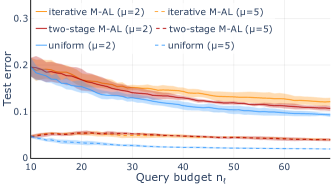
Figure 2: Two-stage M-AL (which we analyze in Section 3.4) is on-par or better than iterative M-AL (Algorithm 1). Data is drawn from the truncated mixture distribution from Section 3.2, with $\mu\in\{2,5\},\sigma=3$ and $d=1000$. Shaded areas indicate standard deviations over 5 runs.

Two-stage margin-based AL.

Similar to other theoretical analyses of active learning [28, 6] we modify Algorithm 1 slightly, and develop the theory instead for a two-stage procedure: 1) we obtain $\hat{\theta}_{seed}$ using the initial small seed set; and 2) we use $\hat{\theta}_{seed}$ to select a batch of $(1-\rho)n_{\ell}$ samples to query from the unlabeled set. This two-stage process avoids the dependence of the classifier at stage $n$ on the unlabeled dataset. chaudhuri15 [6] argue that two-stage strategies are asymptotically not worse than iterative strategies for MLE estimators. Moreover, mussmann18 [28] show that theoretically analyzing this two-stage strategy can reveal insights about iterative AL strategies that are confirmed by experiments on real-world data. In our setting as well, experiments with the two-stage strategy in Figure 2 follow closely the same trends as iterative M-AL.

3 Theoretical analysis of margin-based AL in high dimensions

In this section we give rigorous intuition for the failure of M-AL for high-dimensional logistic regression. In particular, we prove that two-stage M-AL is less sample efficient than PL. Since two-stage M-AL is empirically on-par or better than iterative M-AL in the setting that we consider (Figure 2), our theory gives insights into the failure of the strategy in Algorithm 1. To rule out the cold start problem as a potential cause of this phenomenon, we prove that M-AL also fails when using the Bayes optimal decision boundary for sampling (oracle M-AL), a strategy that is more favorable than M-AL in low-dimensions.

3.1 Logistic regression and the max-$\ell_{2}$-margin solution

We consider linear models of the form $f(x;\theta)=\langle\theta,x\rangle$ with $\theta$ in a fixed-norm ball and minimize the logistic loss, i.e. $\mathcal{L}(z,y)=\log(1+e^{-zy})$. We note that for linearly separable data, minimizing the logistic loss with gradient descent recovers the max-$\ell_{2}$-margin (interpolating) solution [41, 22]. The generalization behavior of this interpolating estimator has been analyzed extensively in recent years in different contexts [2, 21, 29, 8]. In what follows, we refer to the max-$\ell_{2}$-margin classifier trained on a labeled dataset acquired (i) via uniform sampling ($n_{\text{seed}}=n_{\ell}$) as $\hat{\theta}_{unif}$ and (ii) via oracle and empirical M-AL respectively as $\hat{\theta}_{oracle}$ and $\hat{\theta}_{margin}$.

3.2 Data distribution

We now introduce the family of joint data distributions $\mathbb{P}$ for our theoretical analysis that includes distributions where the covariates follow a Gaussian or mixture of truncated Gaussians distribution. These distributions can adequately approximate data generated in many practical applications [4] and have often been considered in theoretical analyses of machine learning algorithms [43, 25, 13].

Noiseless and balanced observations.

Recall that for linear classifiers, the intuitive reason for the effectiveness of M-AL sampling is that after only a few queries, it selects points in the neighborhood of the optimal decision boundary. Notice that this region is where the label noise is concentrated, for a Gaussian mixture model. Therefore, M-AL is prone to query numerous noisy samples. We wish to show the failure of M-AL even in the most benign setting. Hence, we assume a noiseless binary classification problem where the Bayes error vanishes, i.e. $\text{Err}(\theta^{\star})=0$ for some $\theta^{\star}$ unique up to scaling and in this section we set $\|\theta^{\star}\|_{2}=1$. More precisely, we assume that the joint distribution $\mathbb{P}$ is such that the labels $y=\operatorname{sgn}(\langle\theta^{\star},x\rangle)\in\{-1,1\}$ with $\theta^{\star}\in\mathbb{R}^{d}$. For ease of exposition, we assume without loss of generality that $\theta^{\star}=e_{1}=[1,0,...,0]$; if $\theta^{\star}\neq e_{1}$ we can rotate and translate the data to get $\theta^{\star}=e_{1}$ (see Appendix A.1 for more details). We can then rewrite the covariates as $x=[x_{1},\tilde{x}]$ to distinguish between a signal $x_{1}\in\mathbb{R}$ and non-signal component $\tilde{x}\in\mathbb{R}^{d-1}$. Further, to disentangle from phenomena stemming from imbalanced data, we consider a distribution with equal class proportions in expectation (see Appendix A.2 for a discussion).

We obtain a family of joint distributions satisfying these conditions by sampling $y\in\{+1,-1\}$ each with probability one half, and then sampling from the class-conditional distribution defined by $\mathbb{P}_{x_{1}|y}=\mathcal{N}_{trunc}(y\mu,\sigma^{2},y)$ and $\mathbb{P}_{\tilde{x}|y}=\mathcal{N}(0,I_{d-1})$, where $\mathcal{N}_{trunc}(y\mu,\sigma^{2},y)$ denotes the truncated Gaussian distribution with support $(-\infty,0)$ if $y=-1$ and, respectively, support $(0,\infty)$ if $y=1$. The parameters $\mu,\sigma\geq 0$ denote the mean and standard deviation of the non-truncated Gaussian.

Gaussian marginals.

Further note that by setting $\mu=0$, we recover the marginal Gaussian covariate distribution (also known as a discriminative model) – a popular distribution to prove benefits for active learning [3, 17], as both supervised and semi-supervised learning require large amounts of labeled data to achieve low prediction error, even given infinite unlabeled samples [36].

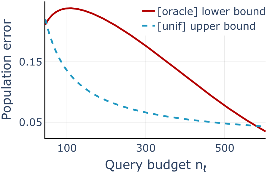
(a) Error vs $n_{\ell}$ (fixed $n_{\text{seed}}$).

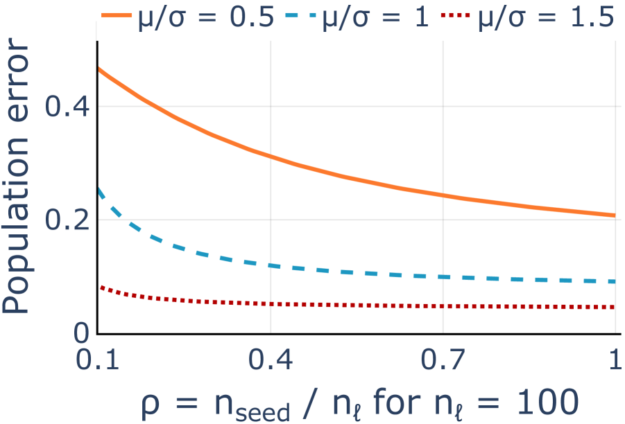
(b) Error vs $\rho$ (fixed $n_{\ell}$).

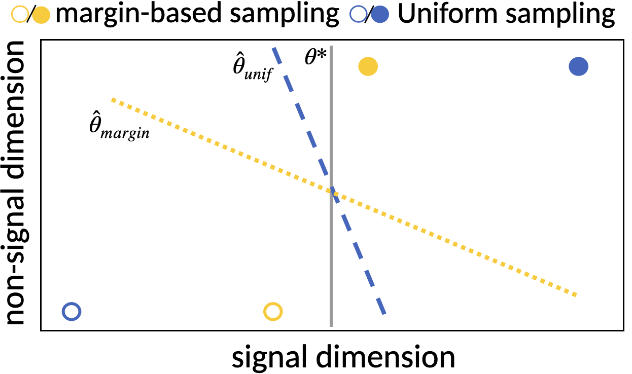
(c) Proof intuition in 2D.

Figure 3: Theoretical population error lower bounds for oracle M-AL and upper bounds for PL in Theorem 3.2 on the truncated Gaussian mixture model. (a) For large $d/n_{\ell}$ the lower bound of Theorem 3.2 on the error of oracle M-AL is much larger than the upper bound on the error of PL for fixed $n_{\text{seed}}=10$ and $\mu/\sigma=1$. (b) The lower bound on the error is smaller when the seed set proportion $\rho$ and the ratio $\mu/\sigma$ are increasing, for fixed $d=1000$ and $n_{\ell}=100$. (c) Intuition for the failure of M-AL in high dimensions. The classifier assigns higher weight to the non-signal dimension when trained on the yellow points close to the optimal decision boundary.

Mixture of truncated Gaussians.

For $\mu>0$, the marginal covariate distribution is a mixture of two truncated Gaussians. Each truncated component has standard deviation $\sigma_{tr}\leq\sigma$ and mean

$$\mu_{tr}:=\mathbb{E}[yx_{1}]=\mu+\sigma\frac{\phi(-\mu/\sigma)}{1-\Phi(-\mu/\sigma)},$$ (1)

where $\mu$ and $\sigma$ determine the non-truncated Gaussian, and $\phi$ and $\Phi$ denote the pdf and the CDF of the standard normal distribution, respectively.

3.3 Warm-up: M-AL versus PL in low dimensions

Before we introduce our main results, we discuss why we expect M-AL to outperform PL for this family of prediction problems. In low-dimensions, mussmann18 [28] show that M-AL requires significantly fewer samples than PL to achieve the same test performance for distributions with vanishing Bayes error – this corresponds to noiseless data. Moreover, in low dimensions and for noiseless data, oracle M-AL further improves the sample complexity, as implied, for instance, by the results in chaudhuri15 [6] (see Appendix A.4.2 for further discussion and an illustrative 1D example). Indeed, experiments on real-world tabular (Figure 1) or image data [37] also confirm that oracle M-AL outperforms M-AL for large labeling budgets. However, we show in the following sections that these intuitions do not transfer to the low-sample regime. Oracle M-AL has not been studied in this setting, prior to our work.

3.4 Main result for high-dimensional M-AL

In this section we present theorems that rigorously prove how logistic regression with margin-based AL leads to worse classifiers in the high-dimensional setting (i.e. $n_{\ell}\ll d$) where most samples are acquired with M-AL (i.e. $\rho\ll 1$) — a phenomenon observed on real-world data in Figure 1-Right. Moreover, we discuss an insight that directly follows from the proof intuition: if many samples in the unlabeled dataset are close to the optimal decision boundary (i.e. small $\mu/\sigma$ ratio), the error gap between M-AL and PL increases. We confirm this intuition on real-world data in Section 4.5.

First, we state the assumptions under which our results hold for high-dimensional active learning. Formal versions of these conditions can be found in the Appendix B.

Assumption 3.1.

Let $n_{\ell}$ be the labeling (or query) budget and $n_{u}$ the unlabeled set size. Assume that $n_{\ell}\ll n_{u}$ and $d\gg n_{\ell}$. Moreover, consider the distribution described in Section 3.2 with $\mu/\sigma<2$, and let $\mathcal{D}_{seed}$ and $\mathcal{D}_{u}$ be datasets drawn i.i.d. from these joint and the marginal distributions, respectively.

Our main results provide lower bounds on the gap between the population error resulting from M-AL versus PL (i.e. uniform sampling). We first state a theorem characterizing this gap for oracle M-AL and refer to Appendix B for the formal statement and proof.

Theorem 3.2 (informal).

Consider the setting introduced in 3.1. Then there exist universal constants $0<c_{1},\epsilon\ll 1$ and $t,c_{2}>0$ such that with probability larger than $1-e^{-c_{2}t^{2}/2}$ it holds that:

$$\text{Err}(\hat{\theta}_{oracle})-\text{Err}(\hat{\theta}_{unif})>\Psi_{\mu,\sigma}\left(\alpha_{\text{oracle}}^{\text{LB}}\right)-\Psi_{\mu,\sigma}\left(\alpha_{\text{unif}}^{\text{UB}}\right),\vspace{-0.1cm}$$

where $\Psi_{\mu,\sigma}$ is a strictly increasing function, defined in Section B.1, and

$$\vspace{-0.3cm}\alpha_{\text{oracle}}^{\text{LB}} =\frac{(1-\epsilon)\sqrt{(d-1)/n_{\ell}}}{\rho\left(\mu_{tr}+t\sigma_{tr}/\sqrt{\rho n_{\ell}}\right)+c_{1}(1-\rho)\mu_{tr}}-1,$$

$$\alpha_{\text{unif}}^{\text{UB}} =\frac{(1+\epsilon)\sqrt{(d-1)/n_{\ell}}}{\mu_{tr}-t\sigma_{tr}/\sqrt{n_{\ell}}}.$$

In particular, if $\rho<\delta$ for $0<\delta<1/2$, then

$$\text{Err}(\hat{\theta}_{oracle})-\text{Err}(\hat{\theta}_{unif})>0.\vspace{-0.1cm}$$

Note that $\Psi_{\mu,\sigma}$ is similar to the cumulative distribution function of the Gaussian distribution (see Appendix B.1 for the exact definition and more details).

A similar result can be proved for two-stage margin-based active learning. We state the theorem informally and defer the formal statement and proof to Appendix B.

Theorem 3.3 (informal).

Consider the setting introduced in 3.1 and further assume that $\sigma>1$. Then there exist universal constants $0<c_{1},\epsilon\ll 1$ and $t,c_{2}>0$ such that with probability larger than $1-e^{-c_{2}t^{2}/2}$ it holds that:

$$\text{Err}(\hat{\theta}_{margin})-\text{Err}(\hat{\theta}_{unif})>\Psi_{\mu,\sigma}\left(\alpha_{\text{margin}}^{\text{LB}}\right)-\Psi_{\mu,\sigma}\left(\alpha_{\text{unif}}^{\text{UB}}\right),$$

where $\Psi_{\mu,\sigma},\alpha_{\text{unif}}^{\text{UB}}$ as in Theorem 3.2 and

$$\alpha_{\text{margin}}^{\text{LB}}=\frac{(1-\epsilon)\sqrt{\frac{d-1}{n_{\ell}}}}{\rho C_{seed}+(1-\rho)\left(c_{1}\mu_{tr}+\sqrt{\frac{\log n_{u}}{C_{seed}}}\sqrt[4]{\frac{(1+\epsilon)(d-1)}{\rho n_{\ell}}}\right)}-1,\vspace{-0.2cm}$$

with $|\mu_{tr}-C_{seed}|<t\sigma_{tr}(\rho n_{\ell})^{-1/2}$. In particular, for small fixed constants $c_{3},c_{4},c_{5}>0$ if $\rho n_{\ell}<c_{3}$, and

$$\mu_{tr}>c_{4}\left(\frac{d-1}{\rho n_{\ell}}\right)^{1/6}(\log n_{u})^{1/3}+\frac{t\sigma_{tr}}{(\rho n_{\ell})^{1/2}},$$

$$\rho<c_{5}\frac{C_{seed}}{\mu_{tr}-\frac{t\sigma_{tr}}{(\rho n_{\ell})^{1/2}}-\left(\frac{d-1}{\rho n_{\ell}}\right)^{1/6}(\log n_{u})^{1/3}},$$

then $\text{Err}(\hat{\theta}_{margin})-\text{Err}(\hat{\theta}_{unif})>0$.

The proof shares the same intuition and key steps as the proof of Theorem 3.2 and differs only in certain technicalities that arise from estimating the classifier $\hat{\theta}_{seed}$. In particular, we additionally need to assume that the mean $\mu_{tr}$ is large enough such that the classifier trained on the seed set has non-trivial prediction error. Note that it is possible to obtain a large $\mu_{tr}$ even for the marginal Gaussian case when $\mu=0$, by choosing a large $\sigma$ in Equation (1).

3.5 Proof sketch and interpretation

In this section we present the intuition behind the proofs of the theorems and discuss the insights revealed by the theory. For simplicity, we focus primarily on Theorem 3.2 for which the phenomenon is more pronounced. We note that the same arguments hold for the setting in Theorem 3.3.

Discussion of assumptions.

We now discuss the conditions needed for the theorems. Observe that if the ratio $\mu/\sigma$ is large, then even PL achieves low error. Hence, we assume settings where $\mu/\sigma<2$, which also cover real-world datasets that contain ambiguous samples that lie near the optimal decision boundary. If $\mu/\sigma<2$ then the covariate distribution has sufficient density in the neighborhood of the optimal decision boundary. Hence, with high probability, the labeled data acquired with M-AL lies in this region, leading to an estimator with high population error. Finally, a small seed set proportion $\rho$ allows for sufficiently many active queries, and is common in situations that employ AL. We refer to Appendix A for further arguments supporting the practical relevance of the setting.

Proof intuition.

Figure 3(c) illustrates the intuition behind the failure of M-AL in high dimensions using a 2D cartoon. We depict the samples chosen by oracle M-AL (yellow), which lie close to the optimal decision boundary (vertical line) and the points selected by uniform sampling (blue), which are farther away from the optimal decision boundary. Note that for both sampling strategies, the selected samples are far apart in the non-signal direction. More specifically, in high dimensions the large distance in the non-signal components $\tilde{x}$ is a consequence of sampling $\tilde{x}$ from a multivariate Gaussian. It follows from these facts that the max-$\ell_{2}$-margin classifier trained on the samples near the optimal decision boundary (yellow dotted) is more tilted (and hence, has larger population error) than the one trained on uniformly sampled points that are further away (blue dashed).

Interpretation of theoretical results.

Theorem 3.2 characterizes when the population error gap between oracle M-AL and PL is positive: for small labeling budgets (leading to a large $d/n_{\ell}$ ratio), for a small seed set proportion ($\rho\ll 1$) and for sufficiently many unlabeled samples near the Bayes optimal decision boundary (implied by $\mu/\sigma<2$). In particular, in the regime $d/n_{\ell}\to\infty$ that implies ${\epsilon}\to 0$ (as argued in Appendix B.2), we can observe how for small $\rho\approx 0$, it holds that $\alpha_{\text{oracle}}^{\text{LB}}\gg\alpha_{\text{unif}}^{\text{UB}}$ as $0<c_{1}\ll 1$. In turn, $\alpha_{\text{oracle}}^{\text{LB}}\gg\alpha_{\text{unif}}^{\text{UB}}$ implies $\text{Err}(\hat{\theta}_{oracle})-\text{Err}(\hat{\theta}_{unif})\gg 0$ since $\Psi_{\mu,\sigma}$ is strictly increasing. In Figure 3 we depict how the error bounds, and hence the gap in Theorem 3.2, depend on the three quantities $\rho,d/n_{\ell}$ and $\mu/\sigma$.

In Figure 3(a), we show the dependence of the bound in Theorem 3.2 on $n_{\ell}$ (and hence, $d/n_{\ell}$), for fixed $n_{\text{seed}}=10,d=1000$ and $\mu/\sigma=1$. If the query budget $n_{\ell}$ and the ratio $\rho$ are small (the middle region of the plot on the horizontal axis), we have a large error gap between oracle M-AL and PL. This phenomenon is inherently high-dimensional and stops occurring for large sample sizes $n_{\ell}$ (the right part of the figure). We also identify these regimes in experiments on real-world data in Section 4.4. In Appendix E, we show more evidence that the theoretical bounds closely predict the values from simulations. Note that the bounds are loose for extremely small budgets (left part of the figure).

In Figure 3(b), we vary the seed set size $n_{\text{seed}}$ (and hence, the ratio $\rho$), for fixed $n_{\ell}=100,d=1000$. We observe that increasing the seed set proportion $\rho$ reduces the error of oracle M-AL (note that $\rho=1$ corresponds to PL). We highlight that the dependence of the error on the ratio $\rho$ is not due to the decision boundary used for M-AL becoming more meaningful for larger $\rho$, as conjectured by some prior works [20, 37]: in our case, we sample using the Bayes optimal decision boundary at every querying step. Instead, Theorem 3.2 captures another failure case of M-AL, specific to high-dimensional settings.

Moreover, Figure 3(b) also illustrates the dependence of the error lower bound on the ratio $\mu/\sigma$, for oracle M-AL. In Theorem 3.2, the distribution-dependent ratio $\mu/\sigma$ enters the bounds via the quantity $c_{1}$ which is strictly increasing in $\mu/\sigma$ (the exact dependence of $c_{1}$ on $\mu/\sigma$ is presented in Lemma B.9 in Appendix B). For small $\mu/\sigma$, the error gap between oracle M-AL ($\rho<1$) and PL ($\rho=1$) is large.

Finally, this phenomenon is caused by choosing to label samples close to the Bayes optimal decision boundary, which are, by definition, the points queried with oracle M-AL. This suggests that, perhaps surprisingly, oracle M-AL exacerbates this high-dimensional phenomenon. Indeed, as evident from comparing the bounds in Theorems 3.2 and 3.3, oracle M-AL performs even worse than M-AL that uses the margin of an empirical estimator $\hat{\theta}$. We confirm this intuition on real-world datasets in Appendix G.2.

4 Experiments

In this section, we provide extensive experiments to investigate the ineffectiveness of low-budget margin-based sampling on high-dimensional real-world data. In particular, we train logistic regression with oracle and empirical M-AL on a wide variety of tabular datasets.

4.1 Datasets

We select binary classification datasets from OpenML [44] and from the UCI data repository [9] according to a number of criteria: i) the data should be high-dimensional ($d>100$) with enough samples that can serve as the unlabeled set ($n_{u}>\max(1000,2d)$); ii) linear classifiers trained on the entire data should have high accuracy (which excludes most image or text datasets). A total number of $15$ datasets satisfy these criteria and cover a broad range of applications from finance and ecology to chemistry and histology. We provide more details about the datasets in Appendix F.1.

Like in Section 3, we wish to isolate the effect of high-dimensionality, and hence, we balance the two classes by subsampling the majority class uniformly at random. Thus we remove confounding effects stemming from applying M-AL on imbalanced data [11]. In addition, we mimic the noiseless setting considered in Section 3 using the following procedure: after fitting a linear classifier on the entire dataset, we remove the training samples that are not correctly predicted and use the subsequent smaller subset as the new dataset. We show that, even in the more favorable noiseless setting, M-AL is less efficient than PL in high dimensions. Experiments on the original, uncurated datasets presented in In Appendix G.1 reveal a similar trend.

4.2 Methodology

We split each dataset into a test and training set. In all experiments, we sample a labeled seed set $\mathcal{D}_{seed}$ of fixed size $n_{\text{seed}}=6$ from the training set (see Appendix G.7 for experiments with larger $n_{\text{seed}}$). The covariates of the remaining training samples constitute the unlabeled set $\mathcal{D}_{u}$.

In practice, one seeks to find the sampling strategy that performs best for a fixed seed set $\mathcal{D}_{seed}$ and labeling budget $n_{\ell}$. To provide an extensive experimental analysis, in this work we compare M-AL (Algorithm 1) and PL over a large number of configurations of $(\mathcal{D}_{seed},n_{\ell})$. We repeatedly draw different seed sets uniformly at random (10 or 100 draws, depending on the experiment) and consider all integer values in $[n_{\text{seed}},d/4]$ as the labeling budget $n_{\ell}$, where $d$ is the ambient dimension of the dataset.

At each querying step, we use L-BFGS [26] to train a linear classifier by minimizing the average logistic loss on the labeled dataset collected until then. Appendix G.6 shows the same high-dimensional phenomenon for $\ell_{1}$- or $\ell_{2}$-regularized classifiers.

4.3 Evaluation metrics

We compare margin-based active learning and passive learning with respect to two performance indicators. On the one hand, we measure the probability that PL leads to a smaller test error than M-AL. The probability is over repeated trials with different seed samples. We compute this probability for each labeling budget $n_{\ell}\in[n_{\text{seed}},d/4]$. On the other hand, we wish to quantify the magnitude of the failure of M-AL. We compare the most significant gains of M-AL with its most significant losses across small query budgets for which PL outperforms M-AL with high probability. In particular, we focus on query budgets smaller than the dataset-dependent transition point $n_{\text{transition}}$, where $n_{\text{transition}}$ is the largest query budget $n_{\ell}\in[n_{\text{seed}},d/4]$ for which the probability of PL outperforming M-AL exceeds $50\%$. If no such budget exists, $n_{\text{transition}}=d/4$. For each query budget size $n_{\ell}\in\{n_{\text{seed}},...,n_{\text{transition}}\}$, we then compute the gap between the test error obtained with M-AL and with PL, over $100$ draws of the seed set. For every labeling budget $n_{\ell}$ we report the largest loss of M-AL (i.e. $95^{th}$ percentiles over the draws of $\mathcal{D}_{seed}$ of the error gap $\text{Err}(\hat{\theta}_{margin})-\text{Err}(\hat{\theta}_{unif})$) and the largest gain of M-AL (i.e. $95^{th}$ percentiles of the error gap $\text{Err}(\hat{\theta}_{unif})-\text{Err}(\hat{\theta}_{margin})$). Then, we depict the distribution of these values of extreme losses/gains over $n_{\ell}\in\{n_{\text{seed}},...,n_{\text{transition}}\}$. In Appendix G.3 and G.5, we present more evaluation metrics (e.g. the dependence of the test error on the budget $n_{\ell}$), which provide further evidence that M-AL fails to be effective in high dimensions.

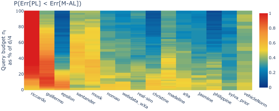
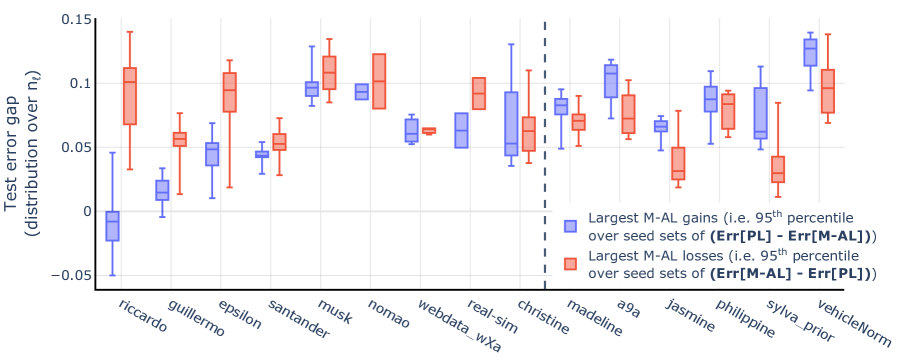
Figure 4: Top: The probability that the test error is lower with PL than with M-AL, over $100$ draws of the seed set. PL outperforms M-AL for a significant fraction of $n_{\ell}\in[n_{\text{seed}},d/4]$ (i.e. warm-colored regions). See Appendix G.4 for more precise numerical values. Bottom: Largest gains and losses in test error of M-AL versus PL, over $100$ draws of $\mathcal{D}_{seed}$. Box plots show distribution over $n_{\ell}\in[n_{\text{seed}},n_{\text{transition}}]$. The sporadic gains of M-AL over PL are generally lower (to left of dashed line) or similar to the losses in test error that it can incur.

4.4 Main results

In Figure 4-Top we show the probability (over $100$ draws of the seed set) that PL leads to lower test error than M-AL. The observations match the trend predicted by our theoretical results (see Theorem B.4): decreasing the seed set ratio $\rho$ (here, by increasing the budget $n_{\ell}$ along the y-axis) leads to a higher probability that PL outperforms M-AL. Analogous to the discussion in Section 3.5, we observe two regimes: for small query budgets $n_{\ell}$, M-AL performs poorly with probability larger than $50\%$ (warm-colored regions). This regime spans a broad range of budgets $n_{\ell}\in[n_{\text{seed}},d/4]$ for most datasets. In the second regime, M-AL eventually outperforms PL for large query budgets.

Furthermore, Figure 4-Bottom shows that in 9 out of 15 datasets, the median (over budgets $n_{\ell}\in[n_{\text{seed}},n_{\text{transition}}]$) of the largest gain of M-AL is lower than the median loss it can incur, compared to PL. Intuitively, this indicates that even in the unlikely event that M-AL leads to better accuracy, the largest gains we can achieve are lower than the potential losses. While the severity of the phenomenon varies with the dataset, we can conclude after this extensive study that margin-based AL cannot be used reliably when the dimension of the data exceeds the size of the query budget.

Finally, recall that in Section 3 and in Figure 1 we show theoretically and empirically that using the margin of the Bayes optimal classifier exacerbates the failure of M-AL in high dimensions. In fact, oracle M-AL performs consistently much worse than both PL and vanilla M-AL in experiments, as indicated in Appendix G.2.

4.5 Verifying trends predicted by theory for M-AL

The intuition developed in Section 3 suggests that the performance of M-AL in high dimensions may improve for: i) a larger separation margin between classes (modeled by $\mu/\sigma$ in the theorems); or ii) a larger seed set (leading to a larger ratio $\rho=n_{\text{seed}}/n_{\ell}$). We test whether these insights also underlie the phenomenon observed in real-world datasets.

First, we investigate the role of the separation margin. We train a linear classifier on the full labeled dataset. Then, we artificially increase the distance between the classes by removing the 25% or 50% closest samples to the decision boundary determined by the classifier trained on the entire dataset. Indeed, we confirm that removing the 25% or 50% most "difficult" samples improves the performance of M-AL significantly as we show in Figure 5, which is in line with the findings of sorscher2022 [40]. In particular, after removing the points close to the Bayes optimal decision boundary, M-AL outperforms PL even on riccardo, the most challenging dataset in our benchmark for AL.

Further, we analyze the impact of a larger seed set size on the performance of M-AL. For a fixed labeling budget $n_{\ell}$, increasing $n_{\text{seed}}$ corresponds to a larger ratio $\rho$, which leads to a smaller gap in error between M-AL and PL as we explain in Section 3: Indeed, we observe that larger seed set sizes can lead to more effective margin-based AL both on synthetic experiments in Figure 8 and on real-world data in experiments presented in Appendix G.7.

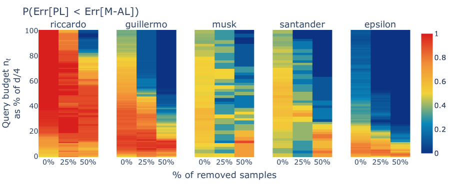
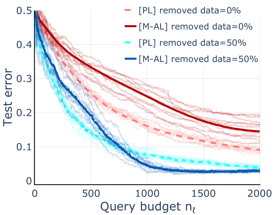
Figure 5: Increasing the separation between the classes in the unlabeled dataset improves the performance of M-AL. Removing the $25\%$ or $50\%$ closest points to the Bayes optimal decision boundary improves M-AL (left) which now outperforms PL for many query budgets (i.e. lighter colors), and even on challenging datasets like riccardo (right).

4.6 Other AL methods in high dimensions and potential mitigations

AL strategies effectively equivalent to M-AL.

Finally, we note that the same failure case occurs for other algorithms, such as margin-based active learning [33, 10, 27] or entropy sampling [38], since they effectively sample the same points as M-AL.

Combining informativeness and representativeness.

Recall that, by definition, varying the ratio $\rho$ modulates the fraction of the labeling budget selected with margin-based sampling, with $\rho=1$ corresponding to PL. Another way to interpolate between M-AL and PL is via a strategy that combines informativeness (via margin-based sampling) and representativeness (via uniform sampling), as proposed by brinker03 [5, 20, 48, 14, 39, 12] We analyze an $\epsilon$-greedy scheme that also falls in this family of AL algorithms: at each querying step, we perform margin-based sampling with probability $1-{\epsilon}$ and uniform sampling with probability $\epsilon$. In Appendix G.8 we provide evidence that PL continues to surpass AL for a large fraction of the labeling budgets, even when using the $\epsilon$-greedy strategy. The intuition for the failure of these algorithms in high dimensions is the same as the one presented in Section 3.

AL with no margin-based sampling.

Could it be that AL algorithms not relying on any form of margin-based score, such as sener18 [37, 15, 16], mitigate this high-dimensional phenomenon? Indeed, we show experimentally in Figure 21 that coreset-based AL [37] outperforms M-AL with high probability in real-world applications. However, compared to PL, the coreset method is still often worse (Figure 22), that is, the high-dimensional phenomenon outlined in Section 3 still persists to a large extent. In particular, no mechanism prevents the coreset strategy from selecting points close to the Bayes optimal decision boundary. As highlighted in Figure 5, selecting these “difficult” samples can hurt the performance of AL.

Discussion on mitigations.

Figure 5 suggests that M-AL constrained to points far enough from the Bayes optimal decision boundary might outperform PL in high dimensions. As the Bayes optimal predictor is not available during training, the closest derived mitigation strategy would be to not allow selecting the points closest to the decision boundary determined by the empirical estimator $\hat{\theta}$ (instead of the optimal $\theta^{\star}$). We find that this mitigation strategy does not help to alleviate the negative effect of M-AL, as it does not effectively remove all the difficult points from the set of query candidates. We regard it as important future work to investigate whether an AL strategy can be provably effective in high-dimensional settings similar to ours.

5 Discussion and future work

In this work we show theoretically and through extensive experiments that active learning, and in particular margin-based sampling, performs worse than uniform sampling for linear models in high dimensions. While we focus on logistic regression and the max-$\ell_{2}$-margin solution, we conjecture that the same intuition outlined in Section 3 holds for other linear predictors like lasso- or ridge-regularized estimators, as indicated by experiments in Appendix G.6.

Moreover, this phenomenon is more general and also occurs for complex non-linear models like deep neural networks. Our experiments suggest that M-AL performs poorly in the context of deep learning on a number of different image classification tasks (see Appendix H), corroborating previous findings by sorscher2022 [40, 16]. We leave as future work an investigation of whether the insights revealed by our analysis of linear models transfers to non-linear predictors like deep neural networks.

Furthermore, for practical purposes, an important question for future work is whether it is possible to construct a strategy that improves upon uniform sampling in high dimensions. Based on Figure 5, we believe that imposing certain conditions on the distributions (e.g. vanishing mass close to the decision boundary) could allow for improvements via active learning.

Appendix A Discussion of assumptions for the theory

In this section we motivate some of the assumptions made in Section 3. We argue why these assumptions are not too constraining and are applicable to a wide variety of practically relevant settings.

A.1 Extension to arbitrary Bayes optimal classifier

In Section 3 we introduce the data distribution and consider noiseless labels determined by a Bayes optimal classifier that takes the form $\theta^{\star}=[1,0,...,0]\in\mathbb{S}^{d-1}$, without loss of generality. We stress that we only make this choice to ease the exposition and make the intuition behind the high-dimensional phenomenon more clear. The distinction between the signal and non-signal components is merely used to make it easier to grasp why this high-dimensional phenomenon occurs. All the arguments in our proofs hold true for arbitrary Bayes optimal classifiers, including a possibly rotated $\theta^{\star}$. A simple way to see this is to notice that the intuition in Figure 3(c) holds true even if we apply a rotation to the data and to $\theta^{\star}$: M-AL still tends to sample points close to the Bayes optimal decision boundary (unlike PL), and hence, the classifier trained on this labeled set will likely be very tilted compared to $\theta^{\star}$.

A.2 Balanced data assumption

In imbalanced classification problems, it is known that margin-based active learning tends to sample a more balanced labeled set than uniform sampling [11]. As a consequence, the classifiers trained on these more balanced labeled data tend to have better predictive performance. This phenomenon occurs both in the low-dimensional and in the high-dimensional regimes.

In our analysis, we want to disentangle effects caused by data imbalance (as the one described in ertekin [11]) from phenomena specific to the high-dimensional regime. Therefore, we consider balanced data for most of our analysis. In Appendix G.1 we also provide experiments on imbalanced tabular data and see that the failure of M-AL in high dimensions still occurs, albeit at a lesser extent. We confirm in our experiments that even in this very low sample regime, M-AL tends to select a more balanced labeled set.

A.3 Gaussian mixture models

As we argue in Section 3.2, GMMs are known to model well data generated in numerous practical applications [4], and hence, have often been studied in theoretical analyses of machine learning algorithms [43, 25, 8]. Note that the GMM assumption is not critical for the proofs and similar results can be obtained for other more general distribution families (e.g. sub-exponential)

A.4 M-AL fails even in beneficial settings

In this work we characterize a failure of margin-based active learning. In order to show the extent of this failure case, we wish to prove that it occurs even in scenarios that are believed to be beneficial for active learning. In particular, we consider data with noiseless labels and show that the failure occurs not only for regular M-AL (Algorithm 1), but even for M-AL that uses the margin of the Bayes optimal classifier for sampling.

A.4.1 Noiseless data

M-AL tends to select points that are close to the Bayes optimal decision boundary. For many label noise models (e.g. logistic noise) this is exactly the region of the input space where the noisy data is concentrated. This observation is also true for many practical applications, for instance when label noise is caused by ambiguities between the classes (e.g. an image that could be assigned either the class “wolf” or “dog” because the object is not clear). Therefore, M-AL tends to be vulnerable to wasting the limited query budget on acquiring labels that are likely to be incorrect. In contrast, PL samples uniformly from the data distribution and may be able to overcome this issue.

We want to ensure that the failure that we study in this paper is not linked to the propensity of M-AL to select noisy samples for labeling. Hence, we consider noiseless data in our analyses. Having said that, we point out that our results can be readily extended to settings with label noise and would lead to a more severe failure of M-AL.

A.4.2 Oracle M-AL versus Empirical M-AL

Since we specifically analyze the failure of M-AL in the low-sample regime, one could argue that this drop in performance is due to the cold start problem: we sample queries using a classifier trained on very few labeled points [20, 37, 16]. To rule out this explanation, we show that we identify the same failure for oracle M-AL that uses the Bayes optimal classifier for sampling. In this section we argue why oracle M-AL performs better than M-AL with an empirical classifier in low dimensions. This good performance of oracle M-AL justifies our choice to study it in high dimensions as well. However, we find that in this latter regime, oracle M-AL fails even more severely than M-AL as we explain in Section 3.

In practice, active learning algorithms use a subjective notion of what the informative samples are, connected to the current empirical predictor that can be trained on the labeled data collected so far. However, the optimal sampling strategy may depend on the Bayes optimal classifier, which, of course, is unknown in practical applications. For instance, it follows from results in chaudhuri15 [6] that a strategy akin to oracle M-AL is optimal in the context of maximum likelihood estimators in low dimensions.

We now present another intuitive way to see why oracle M-AL is expected to need significantly fewer labeled samples in low dimensions, compared to M-AL. Consider the simple setting of learning thresholds in 1D (i.e. functions $f:[0,1]\rightarrow\{0,1\}$ of the form $f_{t}(x)=\mathbb{1}[x>t]$). Assume the covariates are distributed uniformly in $[0,1]$ and that the labels are noiseless, i.e. there exists $t^{\star}$ such that $y=\mathbb{1}[x>t^{\star}]$ for any $x\in[0,1]$.

We know from standard results in learning theory that uniform sampling requires $O(1/\epsilon)$ labeled samples to reach error at most $\epsilon$. Balcan07 [1] prove that M-AL needs a much smaller labeled set of only $O(\log(1/\epsilon))$ to achieve the same test error. In contrast, oracle M-AL requires only $O(1)$ labeled samples to achieve the same performance: we only need to select the samples closest to the Bayes optimal decision boundary until we acquire points from both classes.

This intuitive argument can be extended to dimensions larger than 1 as well. Empirical observations like the one in sener18 [37] corroborate this intuition: oracle M-AL outperforms M-AL in the context of neural networks trained on image data.

It is important to note that in the discussion in this section we rely on a labeling budget much larger than the dimensionality. Prior to our work, the behavior of oracle M-AL has not been studied in the low-sample regime. Therefore, it is justified to ask how oracle M-AL behaves in the high-dimensional regime.

Appendix B Formal statements and proofs of the main results

In this section we state and give the proofs of the main results. We first discuss some preliminaries regarding the mixture of truncated Gaussians distribution after which we state the formal results and the proofs.

B.1 Properties of a mixture of truncated Gaussians

Recall that we consider data drawn from a multivariate mixture of two Gaussians, and we partition the covariates into noise dimensions $\tilde{x}\in\mathbb{R}^{d-1}$ sampled according to $\mathbb{P}_{\tilde{x}}=\mathcal{N}(0,I_{d-1})$ and a signal dimension $x_{1}\in\mathbb{R}$. As detailed in Section 3.2, the signal $x_{1}$ is drawn from a univariate mixture of two Gaussians with means $-\mu$ and $\mu$ for $\mu\in\mathbb{R}$ and standard deviation $\sigma>0$. The components correspond to one of two classes $y\in\{-1,1\}$, and they are truncated such that the data is noiseless. We denote the univariate truncated Gaussian mixture distribution by $\mathbb{P}_{\text{TGMM}}(\mu,\sigma)$ and observe that it determines, by definition, the joint distribution $\mathbb{P}_{yx_{1}}$. To state the formal theorems, we now discuss some properties of the univariate distribution $\mathbb{P}_{\text{TGMM}}(\mu,\sigma)$ that will also be used throughout the proofs in this section.

Mean and standard deviation of a univariate truncated Gaussian.

For completeness, we now introduce the known formulas for the mean and standard deviation of a truncated Gaussian random variable. A positive one-sided truncated Gaussian distribution is defined as follows: we restrict the support of a normal random variable with parameters $(\mu,\sigma)$ to the interval $(0,\infty)$. Clearly the mean of the univariate truncated Gaussian is slightly larger than $\mu$ and the standard deviation slightly smaller than $\sigma$. Let $\phi$ be the probability density function of the standard normal distribution and denote by $\Phi$ the cumulative distribution function. Then we find that the mean of a positive one-sided truncated Gaussian distribution is

$$\mu_{tr}=\mu+\frac{\sigma\phi(-\mu/\sigma)}{1-\Phi(-\mu/\sigma)},$$ (2)

and the standard deviation is given by

$$\sigma_{tr}=\sigma\left(1-\frac{\mu}{\sigma}\cdot\frac{\phi(-\mu/\sigma)}{1-\Phi(-\mu/\sigma)}-\left(\frac{\phi(-\mu/\sigma}{1-\Phi(-\mu/\sigma)}\right)^{2}\right).$$

Error of a linear classifier.

We now derive the closed form of the population error of a linear classifier evaluated on data drawn from a distribution with $\mathbb{P}_{yx_{1}}=\mathbb{P}_{\text{TGMM}}(\mu,\sigma)$ and $\mathbb{P}_{\tilde{x}|y}=\mathcal{N}(0,I_{d-1})$. Consider without loss of generality a classifier induced by a vector $\theta\in\mathbb{R}^{d}$, with $\theta=[1,\alpha\tilde{\theta}]$, where $\|\tilde{\theta}\|_{2}=1$. We use the notation $\alpha(\theta)$ to denote the $\alpha$-parameter of $\theta=[1,\alpha\tilde{\theta}]$. By definition, the error of a classifier $\theta=[1,\alpha\tilde{\theta}]$ is given by

$$\text{Err}_{0-1}(\theta) =\mathbb{P}\left[y\langle\theta,x\rangle<0\right]=\mathbb{P}\left[y\alpha\sum_{i=2}^{d}\tilde{\theta}_{i}x_{i}<-yx_{1}\right]$$ (3)

$$=\frac{1}{2\pi\alpha\sigma(1-\Phi(-\mu/\sigma))}\int_{0}^{\infty}\int_{t}^{\infty}e^{-\frac{(t-\mu)^{2}}{2\sigma^{2}}}e^{-\frac{l^{2}}{2\alpha^{2}}}dldt\eqqcolon\Psi_{\mu,\sigma}(\alpha),$$

where we use the fact that the sum of Gaussian random variables is again a Gaussian random variable, and hence, $y\sum_{i=2}^{d}\theta_{i}x_{i}$ is normally distributed with mean zero and standard deviation $\alpha$. For the final identity, since all coordinates are independent, we use the known formula for the probability density function of a truncated Gaussian.

Note that the expression in Equation (3) can easily be approximated numerically. Moreover, note that $\Psi_{\mu,\sigma}$ resembles the cumulative density function of a standard normal random variable, as illustrated in Figure 6(b): it grows exponentially in $\alpha$, for small values of $\alpha$, and approaches its maximum asymptotically. For convenience we state two properties of the error function $\Psi_{\mu,\sigma}$:

1. $\Psi_{\mu,\sigma}$ is a monotonically increasing function of $\alpha$.

2. $\Psi_{\mu,\sigma}$ is monotonically decreasing in $\mu$.

Therefore, for fixed distributional parameters $\mu$ and $\sigma$, we have that $\alpha$ fully characterizes the error of the classifier. Hence, proving a gap between the values of $\alpha$ obtained with margin-based sampling and with uniform sampling is sufficient to show a gap in the population error.

B.2 Formal statement of Theorem 3.2

In this section, we state the formal version of Theorem 3.2. The proof of the theorem can be found in Section B.4. We start with formally introducing the setting and assumptions. Thereafter, we state the theorem that compares oracle M-AL with PL.

Setting.

We look at the same setting as in Section 3, namely pool based active learning with margin-based sampling strategies. We consider the typical setting where we start with a small labeled dataset $\mathcal{D}_{seed}$ of $n_{\text{seed}}$ samples and a large unlabeled dataset $\mathcal{D}_{u}$ with $n_{u}$ samples all i.i.d. drawn from the truncated Gaussian distribution. We denote by $\rho=\frac{n_{\text{seed}}}{n_{\ell}}$ the fraction of samples we query using uniform sampling. Recall that we define $\hat{\theta}_{unif}$ and $\hat{\theta}_{oracle}$ as the classifiers obtained after querying $(1-\rho)n_{\ell}$ samples either uniformly or with oracle M-AL, respectively.

We now introduce some assumption on the setting. In practice, an unlabeled dataset is available that is much larger than the number of queries. Moreover, most real-world datasets contain some hard examples that are difficult to classify even by human experts. The equivalent synthetic counterpart is the existence of unlabeled samples close to the Bayes optimal decision boundary. Finally, we consider high-dimensional settings, where the dimensionality is larger than the labeling budget. To state our theorem formally, we make these conditions precise in the following assumption.

Assumption B.1.

We assume that $n_{u}>\max(10^{3}n_{\ell},10^{5})$, $\mu/\sigma<2$ and $d-1>n_{\ell}$.

With Assumption B.1, we are now ready to state the theorem.

Theorem B.2 (Oracle margin-based sampling).

For a small constant $c>0$ independent of the dimension and under Assumption B.1, it holds with probability at least $0.99(1-2e^{-t^{2}/2})^{5}(1-e^{-cd/n_{\ell}})$ that:

$$\text{Err}(\hat{\theta}_{oracle})-\text{Err}(\hat{\theta}_{unif})\geq\Psi_{\mu,\sigma}(\alpha_{\text{oracle}}^{\text{LB}})-\Psi_{\mu,\sigma}(\alpha_{\text{unif}}^{\text{UB}}),$$

where

$$\alpha_{\text{unif}}^{\text{UB}}=\frac{\sqrt{\frac{d-1}{n_{\ell}}+\frac{2t}{\sqrt{n_{\ell}}}}}{\mu_{tr}-t\sigma_{tr}n_{\ell}^{-1/2}}, \alpha_{\text{oracle}}^{\text{LB}}=\frac{\sqrt{\frac{d-1}{n_{\ell}}}-1-t}{\rho(\mu_{tr}+t\sigma_{tr}(\rho n_{\ell})^{-1/2})+(1-\rho)6.059\cdot 10^{-2}\mu_{tr}}-1.$$

We note that $\alpha_{\text{unif}}^{\text{UB}},\alpha_{\text{oracle}}^{\text{LB}}$ are upper and lower bounds of $\alpha(\hat{\theta}_{unif})$ and $\alpha(\hat{\theta}_{oracle})$, respectively. The term $(1-e^{-cd/n_{\ell}})$ lower bounds the probability that all points of each sampling strategy are support points (see Lemma B.8 for the explicit probability) – in particular, as the ratio $\frac{d}{n_{\ell}}$ grows, this probability grows. Another consequence of Theorem B.2 is that for high-dimensional data (i.e. $d\gg n_{\ell}$) and for a small ratio of uniformly sampled seed points $\rho\ll 1$, it holds with high probability that $\text{Err}(\hat{\theta}_{oracle})-\text{Err}(\hat{\theta}_{unif})>0$. We state this observation precisely in Corollary B.3 and prove it in Section D.3. To state the corollary, we first define a quantity that is independent of the dimension. Denote by $M_{oracle}$ the denominator of $\alpha_{\text{oracle}}^{\text{LB}}$, i.e. $M_{oracle}=\rho(\mu_{tr}+t\sigma_{tr}(\rho n_{\ell})^{-1/2})+(1-\rho)6.059\cdot 10^{-2}\mu_{tr}$. Note that $M_{oracle}\ll\mu_{tr}$. We are now ready to state the corollary.

Corollary B.3.

Under the same assumptions and with the same probability as in Theorem B.2 it holds that $\text{Err}(\hat{\theta}_{oracle})-\text{Err}(\hat{\theta}_{unif})>0$ if

$$\frac{d-1}{n_{\ell}}>4\left(1+M_{oracle}+t+\sqrt{t(4n_{\ell})^{-1/2}}\right)^{2}, \rho<\frac{1}{2}-\frac{1+\sqrt{2}}{2}\frac{t\sigma_{tr}}{\sqrt{n_{\ell}}\mu_{tr}}.$$

The condition on $\rho$ ensures that enough samples are queried using oracle M-AL such that the difference to passive learning is large enough.

We obtain the first informal statement in Theorem 3.2 directly from Theorem B.2 by choosing

$$\epsilon=\max\left(\sqrt{\frac{n_{\ell}}{d-1}}(1+t),\sqrt{1+\frac{2tn_{\ell}^{1/2}}{d-1}}-1\right),$$ (4)

and the constants $c_{1},c_{2}$ correspondingly. The second statement then follows from Corollary B.3.

B.3 Formal statement of Theorem 3.3

In this section, we state the formal version of Theorem 3.3 which shows an error gap between passive learning and active learning using the margin of the empirical classifier $\hat{\theta}$. Before we state the theorem, we first discuss two-stage margin-based sampling, a slight modification of Algorithm 1.

Two-stage margin-based sampling.

We consider the same modification of the margin-based sampling procedure as [6, 28]. Instead of the iterative process of labeling a point and updating the estimator $\hat{\theta}$, we use a two-stage procedure: 1) we obtain $\hat{\theta}_{seed}$ using the initial small seed set; and 2) we use $\hat{\theta}_{seed}$ to select a batch of $(1-\rho)n_{\ell}$ samples to query from the unlabeled set. Without this two-stage strategy, the estimator $\hat{\theta}$ at a certain iteration is not independent of the unlabeled set, which makes the analysis more challenging, as also noted by [28]. Moreover, chaudhuri15 [6] show that a two-stage strategy similar to ours achieves the optimal convergence rate in the context of maximum likelihood estimators, and hence, it is no worse than the iterative procedure in Algorithm 1. We stress that we do not need this simplification for the analysis of oracle M-AL, since with this strategy the queried points are independent of the estimators $\hat{\theta}$. Moreover, the two-stage procedure is necessary only for one step of the proof highlighted in Section C.2.

We now state the main theorem for empirical M-AL:

Theorem B.4.

For a small constant $c>0$ independent of the dimension and under Assumption B.1 with $\sigma>1$, it holds with probability at least $0.99(1-2e^{-t^{2}/2})^{5}(1-e^{-cd/n_{\ell}})$ that:

$$\text{Err}(\hat{\theta}_{margin})-\text{Err}(\hat{\theta}_{unif})\geq\Psi_{\mu,\sigma}(\alpha_{\text{margin}}^{\text{LB}})-\Psi_{\mu,\sigma}(\alpha_{\text{unif}}^{\text{UB}}),$$

where $\alpha_{\text{unif}}^{\text{UB}}$ is defined as in Theorem B.2 and

$$\alpha_{\text{margin}}^{\text{LB}}=\frac{\sqrt{\frac{d-1}{n_{\ell}}}-\sqrt{2\log n_{u}}-1-t}{\rho C_{seed}+(1-\rho)\left(0.061\mu_{tr}+\sqrt{\frac{2\log n_{u}}{C_{seed}}}\left(\frac{d-1+\sigma_{tr}t}{\rho n_{\ell}}\right)^{1/4}+t\right)}-1,$$

with $C_{seed}$ a constant that satisfies

$$\mu_{tr}-t\sigma_{tr}n_{\text{seed}}^{-1/2}\leq C_{seed}\leq\mu_{tr}+t\sigma_{tr}n_{\text{seed}}^{-1/2}.$$

Theorem B.4 gives a high probability bound for the error gap between passive learning and two-stage empirical margin-based sampling. As before, we state precise conditions when this gap is positive in Corollary B.5 and provide the proof in Section D.4. Similarly as for Corollary B.3, we first define a quantity. Let $M_{margin}$ be the denominator of $\alpha_{\text{margin}}^{\text{LB}}$ and recall that $M_{margin}\ll\mu_{tr}$ if the max-$\ell_{2}$-margin classifier of the seed set $\mathcal{D}_{seed}$ has reasonable accuracy.

Corollary B.5.

Under the same assumptions and with the same probability as in Theorem B.4 it holds that $\text{Err}(\hat{\theta}_{oracle})-\text{Err}(\hat{\theta}_{unif})>0$ if the following conditions are satisfied:

1. (high-dimensional regime) $\frac{d-1}{n_{\ell}}>4\left(\sqrt{2\log n_{u}}+1+M_{margin}+t+\sqrt{t}(4n_{\ell})^{-1/4}\right)$.

2. (large signal-to-noise ratio) $\mu_{tr}\geq\left(\frac{d+\sigma_{tr}t}{\rho n_{\ell}}\right)^{1/6}(\log n_{u})^{1/3}+\frac{t\sigma_{tr}}{(\rho n_{\ell})^{1/2}}$.

3. (numerous margin-based queries) $\rho<\frac{2C_{seed}}{0.878\mu_{tr}-\frac{t\sigma_{tr}}{(\rho n_{\ell})^{1/2}}-\left(\frac{d-1+\sigma_{tr}t}{\rho n_{\ell}}\right)^{1/6}(\log n_{u})^{1/3}-t}$.

The second condition is necessary to ensure that the classifier $\hat{\theta}_{seed}$ trained on the seed set has non-trivial error. Like in Section B.2, the third condition guarantees that the influence of the uniformly sampled seed set is reduced. To get an explicit condition on $\rho$ on the right hand side, we note that $\rho n_{\ell}\geq 2$ by definition.

Furthermore, similar to Section B.2, the term $(1-e^{-cd/n_{\ell}})$ lower bounds the probability that all points are support points for each of the two sampling strategies. The explicit expression for this probability can be found in Lemma B.8.

Finally, observe that Theorem B.4 and Corollary  B.5 are together the formalization of Theorem 3.3. More specifically, by setting $\epsilon$ similar as in Equation (4) and considering large $d/n_{\ell}$, we find the informal statement.

B.4 Proofs of Theorems B.2 and B.4

Recall that, without loss of generality, we consider predictors $\theta=[1,\alpha\tilde{\theta}]$, with $\|\tilde{\theta}\|_{2}=1$, which makes the population error of $\theta$ be a strictly increasing function of $\alpha$. Therefore, to prove Theorems B.2 and B.4 we derive bounds on $\alpha$ for uniform and oracle/empirical margin-based sampling. We split the proof into three main steps. In the first step we bound the $\alpha$-parameter of the max-$\ell_{2}$-margin classifier of a dataset obtained using an arbitrary sampling strategy. The bounds we obtain are a function of certain geometric quantities that we introduce in this section. The second step then bounds these geometric quantities for the specific sampling strategies that we are interested in. Lastly, in the third step we develop these bounds further for the special case of a mixture of truncated Gaussians. Our results also hold for a marginal Gaussian distribution that is usually analyzed in the active learning literature [17].

We would like to reemphasize that we focus on separable data, a setting that benefits active learning. As described in Section 3.2, we consider a Bayes optimal predictor $\theta^{\star}$ with vanishing population error and choose without loss of generality $\theta^{\star}=e_{1}=[1,0,...,0]\in\mathbb{R}^{d}$. We can write the covariates as $x=[x_{1},\tilde{x}]$, where we explicitly separate the coordinates of $x$ into a signal $x_{1}\in\mathbb{R}$ and non-signal component $\tilde{x}\in\mathbb{R}^{d-1}$. The marginal distribution of the covariates takes the form $\mathbb{P}_{X}=\mathbb{P}_{x_{1}}\cdot\mathbb{P}_{\tilde{x}}$, where $\mathbb{P}_{\tilde{x}}=\mathcal{N}(\tilde{x};0,I_{d-1})$ is the distribution of the non-signal dimensions.

We point out that the first two steps of the proof of Theorems B.2 and B.4 hold for any arbitrary distribution $\mathbb{P}_{yx_{1}}$. If the joint distribution $\mathbb{P}_{yx_{1}}$ is a univariate mixture of truncated Gaussians, then $\mathbb{P}_{yx_{1}}=\mathbb{P}_{\text{TGMM}}(\mu,\sigma)$, which in turn corresponds to a marginal Gaussian for $\mu\to 0$.

Step 1: Characterizing $\hat{\theta}$ for arbitrary sampling strategies.

To state the key lemma that characterizes the max-$\ell_{2}$-margin solution $\hat{\theta}$ for any labeled dataset $\mathcal{D}_{\ell}\subset\mathbb{R}^{d}\times\{-1,1\}$ of size $n_{\ell}$, we first introduce three geometric quantities. Recall that we consider classifiers of the form $\theta=[1,\alpha\tilde{\theta}]$ with $\|\tilde{\theta}\|_{2}=1$. We denote the max-$\ell_{2}$-margin of $\mathcal{D}_{\ell}$ in the last $d-1$ coordinates by $\tilde{\gamma}$, and write:

$$\tilde{\gamma}=\max_{\tilde{\theta}\in\mathbb{S}^{d-2}}\min_{(x,y)\in\mathcal{D}_{\ell}}y\langle\tilde{x},\tilde{\theta}\rangle.$$ (5)

Note that $\tilde{\gamma}$ is in fact the maximum min-$\ell_{2}$-margin of $\mathcal{D}_{\ell}$ in the last $d-1$ coordinates. Similarly, the maximum average-$\ell_{2}$-margin of $\mathcal{D}_{\ell}$ in the last $d-1$ coordinates is defined as

$$\tilde{\gamma}_{avg}=\max_{\tilde{\theta}\in\mathbb{S}^{d-2}}\frac{1}{n_{\ell}}\sum_{(x,y)\in\mathcal{D}_{\ell}}y\langle\tilde{x},\tilde{\theta}\rangle.$$ (6)

Lastly, we define the average distance to the decision boundary of the optimal classifier induced by $\theta^{\star}$ as

$$d^{\ast}=\frac{1}{n_{\ell}}\sum_{(x,y)\in\mathcal{D}_{\ell}}yx_{1}.$$

We now state the lemma that bounds the parameter $\alpha$ of the max-$\ell_{2}$-margin classifier trained on an arbitrary labeled set. We provide the proof of the lemma in Section C.1.

Lemma B.6 (Bound on the max-$\ell_{2}$-margin classifier for active learning).

Let $\mathcal{D}_{\ell}$ be a labeled set such that all samples are support vectors of the max-$\ell_{2}$-margin classifier $\hat{\theta}$ of $\mathcal{D}_{\ell}$. Then the $\alpha$-parameter of $\hat{\theta}$ is bounded as follows:

$$\frac{\tilde{\gamma}}{d^{\ast}}-1\leq\alpha\leq\frac{\tilde{\gamma}_{avg}}{d^{\ast}}.$$

Once equipped with Lemma B.6, the next step is to derive bounds on $\tilde{\gamma}$, $\tilde{\gamma}_{avg}$ and $d^{\ast}$ for uniform and oracle/empirical margin-based sampling.

Step 2: Bounding $d^{\ast}$, $\tilde{\gamma}$ and $\tilde{\gamma}_{avg}$ for specific sampling strategies.

In this step, we derive concrete bounds for the key quantities in Lemma B.6 for specific sampling strategies, namely uniform and oracle/empirical margin-based sampling. For this purpose we introduce further geometric quantities that now also depend on the seed set $\mathcal{D}_{seed}$. First, we denote by $d^{\star}_{q}$ the maximal distance of the newly sampled queries to the decision boundary of the Bayes optimal classifier $\theta^{\star}$:

$$d^{\star}_{q}=\max_{(x,y)\in\mathcal{D}_{\ell}\setminus\mathcal{D}_{seed}}yx_{1}.$$

Furthermore, let $\hat{\theta}_{seed}$ be the parameter vector of the max-$\ell_{2}$-margin classifier of the seed set with $\alpha$-parameter $\alpha_{seed}$. We define $\hat{d}_{q}$ as the maximal distance of the newly queried points to the decision boundary determined by $\hat{\theta}_{seed}$:

$$\hat{d}_{q}=\max_{(x,y)\in\mathcal{D}_{\ell}\setminus\mathcal{D}_{seed}}\frac{\left|\langle\hat{\theta}_{seed},x\rangle\right|}{\|\hat{\theta}_{seed}\|_{2}}.$$

Lastly, we define $C_{seed}$ as the average distance to the decision boundary of $\theta^{\star}$ of the samples in the seed set:

$$C_{seed}=\frac{1}{n_{\text{seed}}}\sum_{(x,y)\in\mathcal{D}_{seed}}yx_{1}.$$

Finally, recall that in pool-based active learning one has access to an unlabeled set $\mathcal{D}_{u}$ drawn i.i.d. from $\mathbb{P}_{X}$ and a small labeled seed set $\mathcal{D}_{seed}$ where the covariates are drawn i.i.d. from $\mathbb{P}_{XY}$. We collect a labeled set $\mathcal{D}_{\ell}$ that includes the uniformly sampled $\mathcal{D}_{seed}$ and $(1-\rho)n_{\ell}$ labeled points whose covariates are selected from $\mathcal{D}_{u}$ according to a sampling strategy. We are now ready to state the following lemma, which bounds the quantities that show up in Lemma B.6, namely $d^{\ast}$, $\tilde{\gamma}$ and $\tilde{\gamma}_{avg}$. The proof of the lemma is presented in Section C.2.

Lemma B.7 (Bounds on $d^{\ast}$, $\tilde{\gamma}$ and $\tilde{\gamma}_{avg}$).

Consider the standard pool-based active learning setting in which we collect a labeled set $\mathcal{D}_{\ell}$ and assume $n_{\ell}<d-1<n_{u}$ where $n_{\ell}=|\mathcal{D}_{\ell}|$ and $n_{u}=|\mathcal{D}_{u}|$. Then, the following are true:

1. If $\mathcal{D}_{\ell}$ is collected using uniform sampling, then with a probability greater than $1-2e^{-t^{2}/2}$, it holds that

   $$d^{\ast}=\frac{1}{n_{\ell}}\sum_{(x,y)\in\mathcal{D}_{\ell}}yx_{1}, \tilde{\gamma}_{avg}<\sqrt{\frac{d-1}{n_{\ell}}+\frac{2t}{\sqrt{n_{\ell}}}}.$$ (7)

2. If $\mathcal{D}_{\ell}$ is collected using oracle margin-based sampling, then with probability greater than $1-2e^{-t^{2}/2}$ it holds that

   $$d^{\ast}<\rho C_{seed}+(1-\rho)d^{\star}_{q}, \tilde{\gamma}>\sqrt{\frac{d-1}{n_{\ell}}}-1-t.$$ (8)

3. If $\mathcal{D}_{\ell}$ is collected using two-stage empirical margin-based sampling, then with probability greater than $(1-2e^{-t^{2}/2})^{2}$, it holds that

   $$d^{\ast}<\rho C_{seed}+(1-\rho)(\hat{d}_{q}+\sqrt{2\alpha_{seed}\log n_{u}}+t), \tilde{\gamma}>\sqrt{\frac{d-1}{n_{\ell}}}-\sqrt{2\log n_{u}}-1-t.$$ (9)

Plugging these bounds into the result of Lemma B.6, we find high-probability bounds on the $\alpha$-parameter of each of these three sampling strategies. As explained in Section B.4, these bounds hold for any arbitrary joint distribution of the signal component and the label, $\mathbb{P}_{yx_{1}}$. In what follows we derive the bounds on $\alpha$ further for a mixture of truncated Gaussians.

Step 3: Bounding $d^{\ast},d^{\star}_{q},\hat{d}_{q},\alpha_{\text{seed}}$, $C_{seed}$ and the probability that all samples are support vectors for a mixture of truncated Gaussians.

In order to use Lemma B.7 to prove the theorem, we first derive the probability that all samples in $\mathcal{D}_{\ell}$ are support points for $\mathbb{P}_{yx_{1}}=\mathbb{P}_{\text{TGMM}}(\mu,\sigma)$ for uniform and oracle/empirical margin-based sampling. This result is summarized in Lemma B.8 (see Appendix C.3 for the proof).

Lemma B.8 (All samples are support points).

Let $\mathcal{D}_{\ell}$ be a dataset of $n_{\ell}<d-1$ samples drawn via either uniform sampling, margin-based sampling or oracle margin-based sampling from a large unlabeled dataset. The unlabeled data is drawn i.i.d. from the multivariate mixture of truncated Gaussians distribution. Then, for a constant $c(\mu_{tr},\sigma_{tr},n_{u})>0$ independent of $d$ and $n_{\ell}$ it holds with probability larger than $1-2e^{-(\sqrt{(d-1)/n_{\ell}}-\sqrt{\log n_{\ell}}-c)^{2}}$ that all samples in $\mathcal{D}_{\ell}$ are support points of the max-$\ell_{2}$-margin classifier of $\mathcal{D}_{\ell}$.

Next, we bound $d^{\star}_{q},\hat{d}_{q},\alpha_{\text{seed}}$ and $C_{seed}$ which finalizes the proof. We note that for uniform sampling, $d^{\ast}$ is the average of $n_{\ell}$ i.i.d. samples from a one-sided truncated Gaussian, which is a sub-Gaussian random variable with mean $\mu_{tr}$ and standard deviation $\sigma_{tr}$. Hence, with probability larger than $1-2e^{-t^{2}/2}$, it holds via Hoeffding’s inequality that

$$d^{\ast}>\mu_{tr}-t\sigma_{tr}n_{\ell}^{-1/2}.$$ (10)

By the same argument it holds with probability greater than $1-2e^{-t^{2}/2}$ that

$$C_{seed}<\mu_{tr}+t\sigma_{tr}n_{\text{seed}}^{-1/2}.$$ (11)

To bound the remaining quantities, we treat each of the three sampling strategies separately.

(a) Uniform sampling.

Plugging the bounds on $d^{\ast}$ (Equation (10)) and $\tilde{\gamma}_{avg}$ (Lemma B.7) into Lemma B.6 and multiplying the independent probability statements yields the expression of the upper bound $\alpha_{\text{unif}}^{\text{UB}}\geq\alpha(\hat{\theta}_{unif})$ that appears in Theorems B.2 and B.4.

(b) Oracle margin-based sampling.

We now bound $d^{\star}_{q}$ using the following lemma which we prove in Section D.1.

Lemma B.9 (Bound on $d^{\star}_{q}$).

Let $\mathcal{D}_{u}$ and $\mathcal{D}_{seed}$ be the unlabeled set and the labeled seed set, respectively, with covariates drawn i.i.d. from the multivariate mixture of truncated Gaussians distribution. Then, with probability larger than $1-e^{-t^{2}}$, we have that

$$d^{\star}_{q}<\sigma\left(\Phi^{-1}\left(\left(t(2n_{u})^{-1/2}+(1-\rho)n_{\ell}/n_{u}\right)\left(1-\Phi(-\mu/\sigma)\right)+\Phi(-\mu/\sigma)\right)\right)+\mu.$$

Moreover, if $n_{u}>\max(10^{5},10^{3}n_{\ell})$ and $\mu/\sigma<2$ then with probability greater than 0.99

$$d^{\star}_{q}<6.059\cdot 10^{-2}\mu_{tr}.$$

We now argue that the conditions required for Equation (B.9) to hold are not too restrictive. Indeed, it is standard in practical active learning settings that the unlabeled set is orders of magnitude larger than the labeling budget. Moreover, in most real-world datasets there exist ambiguous samples, close to the optimal decision boundary, which can be be difficult to classify even for human experts. The condition $\mu/\sigma<2$ ensures that that is the case in our setting as well, with high probability.

Invoking the probability bound in Lemma B.8, plugging the bounds on $C_{seed}$ (Equation (11)), $\tilde{\gamma}$ (Lemma B.7) and $d^{\star}_{q}$ (Lemma B.9) into Lemma B.6 gives the expression for lower bound $\alpha_{\text{oracle}}^{\text{LB}}\leq\alpha(\hat{\theta}_{oracle})$ that appears in Theorem B.2. Invoking all the probability statements involved and combining this result with the previous derivation of $\alpha_{\text{unif}}^{\text{UB}}$ finishes the proof of Theorem B.2.

(c) Two-stage margin-based sampling.

For bounding $\hat{d}_{q}$ we can use a similar technique as in Lemma B.9, if we assume further that $\sigma\geq 1$. This condition ensures that, with high probability, there exist examples with a high signal component for any $\mu\geq 0$. The following lemma states the bound on $\hat{d}_{q}$ (see Section D.2 for the proof).

Lemma B.10 (Bound on $\hat{d}_{q}$).

Let $\mathcal{D}_{u}$ and $\mathcal{D}_{seed}$ be the unlabeled set and the labeled seed set, respectively, with covariates drawn i.i.d. from the multivariate mixture of truncated Gaussians distribution. If $\sigma\geq 1$ then it holds with probability larger than $1-e^{-t^{2}}$ that

$$\hat{d}_{q}<\sigma\left(\Phi^{-1}\left(\left(t(2n_{u})^{-1/2}+(1-\rho)n_{\ell}/n_{u}\right)\left(1-\Phi(-\mu/\sigma)\right)+\Phi(-\mu/\sigma)\right)\right)+\mu.$$

Moreover, if $n_{u}>\max(10^{5},10^{3}n_{\ell})$ and $\mu/\sigma<2$ then with probability greater than 0.99

$$\hat{d}_{q}<6.059\cdot 10^{-2}\mu_{tr}.$$

Using Lemma B.10, we now derive an upper bound on $\alpha_{\text{seed}}$. We note that the seed set is drawn i.i.d. from the data distribution. Hence, we can use the bound for uniform sampling of Lemma B.6 and set $\mathcal{D}_{\ell}=\mathcal{D}_{seed}$ to arrive at $\alpha_{\text{seed}}<\tilde{\gamma}_{avg}/d^{\ast}$. By a similar argument, we use the bound of Equation (10) to lower bound $C_{seed}$ and we obtain that $C_{seed}>\mu_{tr}-t\sigma_{tr}(\rho n_{\ell})^{-1/2}$. Then, by Lemma B.7, we have that $\tilde{\gamma}_{avg}<\left(\frac{d-1}{\rho n_{\ell}}+\frac{2t}{(\rho n_{\ell})^{1/2}}\right)^{1/2}$ with probability greater than $1-2e^{-t^{2}/2}$. Note that if all uniform samples are support points of the max-$\ell_{2}$-margin classifier, then all samples in the seed set are as well for the max-$\ell_{2}$-margin classifier of the seed set. Putting everything together, we find that, with probability greater than $(1-2e^{-t^{2}/2})^{2}$, it holds that

$$\alpha_{\text{seed}}\leq\left(\frac{d-1}{\rho n_{\ell}}+\frac{2t}{(\rho n_{\ell})^{1/2}}\right)^{1/2}\left(\mu_{tr}-\frac{t\sigma_{tr}}{(\rho n_{\ell})^{1/2}}\right)^{-1}.$$ (12)

Plugging the bounds on $C_{seed}$ (Equation (11)), $\tilde{\gamma}$ (Lemma B.7) , $\alpha_{\text{seed}}$ (Equation (12)) and $\hat{d}_{q}$ (Lemma B.10) into Lemma B.6 gives the expression for the lower bound $\alpha_{\text{margin}}^{\text{LB}}\leq\alpha(\hat{\theta}_{margin})$ that appears in Theorem B.4. Invoking all the probability statements involved and combining this result with the previous derivation of $\alpha_{\text{unif}}^{\text{UB}}$ finishes the proof of Theorem B.4.

Appendix C Proofs of main Lemmas

In this section, we provide proofs for the lemmas needed to prove the main theoretical results presented in Section B.

C.1 Proof of Lemma B.6

Recall that we can consider parameter vector that are normalized such that

$$\hat{\theta}=[1,\alpha\tilde{\theta}],$$

for some $\alpha\geq 0$ with $\|\tilde{\theta}\|_{2}=1$. Further, recall that we decompose covariates as $x=[x_{1},\tilde{x}]$. For convenience of notation, we define $\bar{a}=\frac{1}{n_{\ell}}\sum_{(x,y)\in\mathcal{D}_{\ell}}y\langle\tilde{\theta},\tilde{x}\rangle$, namely the average margin in the $d-1$ noise dimensions $\tilde{x}$ of points in the dataset $\mathcal{D}_{\ell}$.

From the conditions of the lemma we have that all points in $\mathcal{D}_{\ell}$ are support points. Since, the distance to the decision boundary induced by $\hat{\theta}$ is the same for all support points, we can write the max-$\ell_{2}$-margin $\gamma$ as the following average:

$$\gamma =\frac{1}{\|\hat{\theta}\|_{2}n_{\ell}}\sum_{(x,y)\in\mathcal{D}_{\ell}}\left(yx_{1}+\alpha y\langle\tilde{\theta},\tilde{x}\rangle\right)=\frac{1}{\sqrt{1+\alpha^{2}}}\left(d^{\ast}+\alpha\bar{a}\right).$$

Maximizing over $\alpha$, we find that the max-$\ell_{2}$-margin classifier $\hat{\theta}$ is determined by the following $\alpha$-parameter:

$$\alpha=\frac{\bar{a}}{\frac{1}{n_{\ell}}\sum_{(x,y)\in\mathcal{D}_{\ell}}yx_{1}}=\frac{\bar{a}}{d^{\ast}}.$$

Hence, the max-$\ell_{2}$-margin classifier can be written as $\hat{\theta}=\left[1,\frac{\bar{a}}{d^{\ast}}\tilde{\theta}\right]$ and the margin is given by $\gamma=\sqrt{d^{\ast^{2}}+\bar{a}^{2}}$.

Now we prove that we can use the maximum average-$\ell_{2}$-margin $\tilde{\gamma}_{avg}$ and the max-$\ell_{2}$-margin $\tilde{\gamma}$ in the $d-1$ noise coordinates to sandwich $\bar{a}$ as follows: $\tilde{\gamma}_{avg}\geq\bar{a}\geq\sqrt{\tilde{\gamma}^{2}-d^{\ast^{2}}}$.

The first inequality follows directly from the definition of the maximum average-$\ell_{2}$-margin $\tilde{\gamma}_{avg}$ in Equation (6). We now prove the second inequality. Let $\tilde{\theta}_{\text{MM}}$ be the max-$\ell_{2}$-margin classifier in the $d-1$ noise coordinates, with $\|\tilde{\theta}_{\text{MM}}\|_{2}=1$. By the definition of $\tilde{\theta}_{\text{MM}}$, it holds that $y\langle\tilde{\theta}_{\text{MM}},\tilde{x}\rangle\geq\tilde{\gamma}$. Moreover, consider the classifier determined by $\theta=[\min_{(x,y)\in\mathcal{D}_{\ell}}yx_{1},\tilde{\gamma}\tilde{\theta}_{\text{MM}}]\in\mathbb{R}^{d}$. Since the max-$\ell_{2}$-margin $\gamma$ is maximal it holds that

$$\gamma\geq\min_{(x,y)\in\mathcal{D}_{\ell}}\frac{y\langle\theta,x\rangle}{\|\theta\|_{2}}\geq\sqrt{\left(\min_{(x,y)\in\mathcal{D}_{\ell}}yx_{1}\right)^{2}+\tilde{\gamma}^{2}}.$$

Using that $\gamma=\sqrt{d^{\ast^{2}}+\bar{a}^{2}}$, and solving for $\bar{a}$, we find that

$$\alpha=\frac{\bar{a}}{d^{\ast}}\geq\frac{\sqrt{\tilde{\gamma}^{2}+\left(\min_{(x,y)\in\mathcal{D}_{\ell}}yx_{1}\right)^{2}-d^{\ast^{2}}}}{d^{\ast}}\geq\frac{\tilde{\gamma}}{d^{\ast}}-1,$$

which concludes the proof.

C.2 Proof of Lemma B.7

Lemma B.7 consists of three statements: a lower bound on the value of $\alpha$ for margin-based sampling and for oracle margin-based sampling, and an upper bound on $\alpha$ for passive learning.

Recall that by Lemma B.6 we have that for a labeled set $\mathcal{D}_{\ell}$ collected through any sampling strategy, the $\alpha$-parameter of the max-$\ell_{2}$-margin classifier of $\mathcal{D}_{\ell}$ is lower and upper bounded by

$$\frac{\tilde{\gamma}}{d^{\ast}}-1\leq\alpha\leq\frac{\tilde{\gamma}_{avg}}{d^{\ast}},$$

where $d^{\ast}=\frac{1}{n_{\ell}}\sum_{(x,y)\in\mathcal{D}_{\ell}}yx_{1}$. To prove Lemma B.7, we apply Lemma B.6 and bound $\tilde{\gamma},\tilde{\gamma}_{avg}$ and $d^{\ast}$ for each sampling strategy separately.

C.2.1 Key margin results

To prove Lemma B.7 we need to bound the $\ell_{2}$-margin in the $d-1$ noise coordinates of a dataset. In this section we give high probability bounds for the $\ell_{2}$-margin, which hold if the conditions of Lemma B.7 are satisfied, i.e. the max-$\ell_{2}$-margin classifier exists.

Lemma C.1 (Bounds for margins $\gamma,\gamma_{avg}$.).

Let $\mathcal{D}$ be a dataset of size $n<d$ with i.i.d. inputs $x\sim\mathcal{N}(0,\mathbb{I}_{d})$ and arbitrary labels such that the max-$\ell_{2}$-margin solution exists. Then it holds with probability at least $1-2e^{-t^{2}/2}$ that

• the maximum average-$\ell_{2}$-margin $\gamma_{avg}$ of $\mathcal{D}$ is upper bounded by

  $$\gamma_{avg}\leq\sqrt{\frac{d}{n}+\frac{2t}{\sqrt{n}}}.$$ (13)

• the max-$\ell_{2}$-margin $\gamma$ of $\mathcal{D}$ is upper and lower bounded by

  $$\sqrt{\frac{d}{n}}-1-t\leq\gamma\leq\sqrt{\frac{d}{n}}+1+t.$$ (14)

Let $\mathcal{D}$ be a labeled dataset of size $n<d$ where $\{x:(x,y)\in\mathcal{D}\}$ is an arbitrary subset among $n_{u}$ i.i.d. samples $x\sim\mathcal{N}(0,\mathbb{I}_{d})$ with arbitrary labels such that the max-$\ell_{2}$-margin solution exists. Then, with probability at least $1-e^{-t^{2}/2}$,

• the max-$\ell_{2}$-margin $\gamma$ of $\mathcal{D}$ is upper and lower bounded by

  $$\sqrt{\frac{d}{n}}-\sqrt{2\log n_{u}}-1-t\leq\gamma\leq\sqrt{\frac{d}{n}}+\sqrt{2\log n_{u}}+1+t.$$ (15)

The proof of the lemma can be found in Section C.4.

C.2.2 Proof of Lemma B.7

We now use Lemma C.1 to prove Lemma B.7. We do so by replacing $\mathcal{D}$ in Lemma C.1 by the set $\tilde{\mathcal{D}}_{\ell}:=\{(\tilde{x},y):(x,y)\in\mathcal{D}_{\ell}\text{, where }x=[x_{1},\tilde{x}]\}$, where $\mathcal{D}_{\ell}$ is collected with one of the three sampling strategies that we consider. By the conditions of Lemma B.7 we have that the max-$\ell_{2}$-margin solution exists.

Uniform sampling

• For uniform sampling, Lemma C.1 directly yields the upper bound for $\tilde{\gamma}_{avg}$: it suffices to replace $\gamma_{avg}$ with $\tilde{\gamma}_{avg}$ to arrive to arrive at $\tilde{\gamma}_{avg}\leq\sqrt{\frac{d-1}{n_{\ell}}+\frac{2t}{\sqrt{n_{\ell}}}}$, which proves Equation (7).

Oracle margin-based sampling

• Bound for $\tilde{\gamma}$. We now argue that the set $\tilde{\mathcal{D}}_{\ell}:=\{(\tilde{x},y):(x,y)\in\mathcal{D}_{\ell}\text{, where }x=[x_{1},\tilde{x}]\}$ satisfies the assumptions of Lemma C.1 when $\mathcal{D}_{\ell}$ is collected with oracle M-AL. The bound on $\tilde{\gamma}$ then follows directly. Note that oracle M-AL queries the $(1-\rho)n_{\ell}$ closest points to the optimal decision boundary. Importantly, the Bayes optimal classifier is independent of the $d-1$ noise coordinates of the covariates. Therefore, $\tilde{\mathcal{D}}_{\ell}$ selected with oracle M-AL is drawn i.i.d. from a standard normal distribution, and hence, satisfies the conditions of Lemma C.1.

  Since, we have that $d>n-1$ and we consider linear classifiers with an intercept at the origin, the max-$\ell_{2}$-margin classifier always exists. Therefore, we are in the conditions of Lemma C.1 and we get that $\tilde{\gamma}\geq\sqrt{(d-1)/n_{\ell}}-1-t$ with probability greater than $1-2e^{-t^{2}/2}$.

• Bound for $d^{\ast}$. Next, observe that using the definitions of $\rho=\frac{n_{\text{seed}}}{n_{\ell}}$ and $C_{seed}=\frac{1}{n_{\text{seed}}}\sum_{(x,y)\in\mathcal{D}_{seed}}yx_{1}$ we can write

  $$d^{\ast} =\frac{1}{n_{\ell}}\sum_{(x,y)\in\mathcal{D}_{\ell}}yx_{1}=\rho C_{seed}+\frac{1}{n_{\ell}}\sum_{(x,y)\in\mathcal{D}_{\ell}\setminus\mathcal{D}_{seed}}yx_{1}$$

  $$=\rho C_{seed}+(1-\rho)\frac{1}{n_{\ell}-n_{\text{seed}}}\sum_{(x,y)\in\mathcal{D}_{\ell}\setminus\mathcal{D}_{seed}}yx_{1}\leq\rho C_{seed}+(1-\rho)d^{\star}_{q},$$

  where the inequality follows from the definition of $d^{\star}_{q}:=\max_{(x,y)\in\mathcal{D}_{\ell}\setminus\mathcal{D}_{seed}}yx_{1}$. This concludes the proof of the inequalities in Equation (8).

Empirical margin-based sampling

• Bound for $\tilde{\gamma}$. We argue now that $\tilde{\gamma}$ corresponds to $\gamma$ in Equation (15). In particular, since the inequalities in Equation (15) hold for any subset of $\mathcal{D}_{u}$, they also hold for the set $\mathcal{D}_{\ell}$ collected with empirical margin-based sampling. Therefore, we find that with probability greater than $1-e^{-t^{2}/2}$, the max-$\ell_{2}$-margin in the $d-1$ noise coordinates is lower bounded by $\sqrt{(d-1)/n_{\ell}}-\sqrt{2\log n_{u}}-1-t$.

• Bound for $d^{\ast}$. We stress that this is the only step in the entire proof of Theorem B.4 where we use the two-stage margin-based sampling procedure (instead of the iterative process described in Algorithm 1).

  Similar to oracle margin-based sampling, the key is to derive a bound for $\frac{1}{n_{\ell}-n_{\text{seed}}}\sum_{(x,y)\in\mathcal{D}_{\ell}\setminus\mathcal{D}_{seed}}yx_{1}$. Recall that $\hat{\theta}_{seed}=[1,\alpha_{\text{seed}}\tilde{\theta}_{seed}]$ with $\|\tilde{\theta}_{seed}\|_{2}=1$ is the max-$\ell_{2}$-margin classifier of $\mathcal{D}_{seed}$. Further, due to the two-stage procedure, $\tilde{\theta}_{seed}$ is independent of all the samples in the unlabeled dataset. Using this fact together with the union bound and that the labels are independent of the $d-1$ last coordinates, we find that $\max_{(x,y)\in\mathcal{D}_{u}}\alpha_{\text{seed}}\langle\tilde{\theta}_{seed},y\tilde{x}\rangle<\sqrt{2\alpha_{\text{seed}}\log n_{u}}+t$ Therefore, together with the definition of $\hat{d}_{q}$, we have that with probability greater than $1-2e^{-t^{2}/2}$:

  $$\frac{1}{n_{\ell}-n_{\text{seed}}}\sum_{(x,y)\in\mathcal{D}_{\ell}\setminus\mathcal{D}_{seed}}yx_{1} =\frac{1}{n_{\ell}-n_{\text{seed}}}\sum_{(x,y)\in\mathcal{D}_{\ell}\setminus\mathcal{D}_{seed}}y\langle\hat{\theta}_{seed},x\rangle-\alpha_{\text{seed}}\langle\tilde{\theta}_{seed},y\tilde{x}\rangle$$

  $$\leq\hat{d}_{q}+\sqrt{2\alpha_{seed}\log n_{u}}+t,$$

  from which the bound for $d^{\ast}$ in Equation (15) follows.

C.3 Proof of Lemma B.8

We now prove this lemma for oracle margin-based sampling. The result for the other strategies follows a nearly identical argument if we use the respective bounds on $\tilde{\gamma}$ as in Lemma C.1.

Recall that, by definition, all support points have the same $\ell_{2}$-distance to the decision boundary of the max-$\ell_{2}$-margin classifier, denoted by $\gamma$. Clearly, the max-$\ell_{2}$-margin of $\mathcal{D}_{\ell}$ is lower bounded by the max-$\ell_{2}$-margin in the last $d-1$ coordinates, i.e.

$$\gamma\geq\tilde{\gamma}.$$ (16)

Now, let $D_{s}\subset\mathcal{D}_{\ell}$ be the subset containing all support points, then by Lemma B.6, the normalized max-$\ell_{2}$-margin classifier can be written as follows:

$$\hat{\theta}=\frac{1}{\sqrt{\hat{\theta}_{1}^{2}+a^{2}}}\left[\hat{\theta}_{1},a\tilde{\theta}\right],$$

with $a>\sqrt{\tilde{\gamma}^{2}-\hat{\theta}_{1}^{2}}$ where $\|\tilde{\theta}\|_{2}=1$ and we use the notation $\hat{\theta}_{1}=\frac{1}{\left|D_{s}\right|}\sum_{(x,y)\in D_{s}}yx_{1}$. Therefore, it holds that $\gamma=y\langle\hat{\theta},x\rangle\geq\sqrt{\hat{\theta}_{1}^{2}+\tilde{\gamma}^{2}}=\tilde{\gamma}$ for all $(x,y)\in D_{s}$. After rewriting it follows that $\mathcal{D}_{\ell}\subseteq D_{s}$, if the following condition is satisfied:

$$\max_{(x,y)\in\mathcal{D}_{\ell}}\tilde{\gamma}y\langle\tilde{\theta},\tilde{x}\rangle\leq\gamma^{2}-y\hat{\theta}_{1}x_{1}.$$ (17)

We now take steps to give a more restrictive sufficient condition that implies the one in Equation (17), and hence, also implies that $\mathcal{D}_{\ell}\subseteq D_{s}$. For an arbitrary pair $(x,y)\in\mathcal{D}_{\ell}\setminus\mathcal{D}_{seed}$ the following inequality holds with a probability larger than $1-2e^{-t^{2}/2}$:

$$\tilde{\gamma}^{2}-y\hat{\theta}_{1}x_{1} \overset{i}{\geq}\tilde{\gamma}^{2}-y\hat{\theta}_{1}x_{1}$$

$$\overset{ii}{\geq}\tilde{\gamma}^{2}-y\hat{\theta}_{1}(\mu_{tr}+t\sigma_{tr})$$

where inequality (i) follows from Equation (16) and (ii) holds as $d^{\star}_{q}<\mu_{tr}$ and the concentration bound in the first coordinate of uniformly sampled queries. Now, note that $\hat{\theta}_{1}\leq\mu_{tr}+t\sigma_{tr}=c(\mu_{tr},\sigma_{tr})$. Hence, for all samples in $\mathcal{D}_{\ell}\setminus\mathcal{D}_{seed}$ to be support points it is sufficient that the following holds:

$$\max_{(x,y)\in\mathcal{D}_{\ell}\setminus\mathcal{D}_{seed}}\tilde{\gamma}y\langle\tilde{\theta},\tilde{x}\rangle\leq\tilde{\gamma}^{2}-c(\mu_{tr},\sigma_{tr})^{2}.$$

Since $\tilde{x}$ is distributed according to a multivariate standard Gaussian and $\|\tilde{\theta}\|_{2}=1$, we know that

$$\max_{(x,y)\in\mathcal{D}_{\ell}\setminus\mathcal{D}_{seed}}y\langle\tilde{\theta},\tilde{x}\rangle\leq\sqrt{2\log n_{\ell}}+t,$$

with probability at least $1-2e^{-t^{2}/2}$. By combining Equations (C.3) and (C.3), we get that $\mathcal{D}_{\ell}\setminus\mathcal{D}_{seed}\subseteq D_{s}$ with probability at least $1-2e^{-0.5\left(\tilde{\gamma}-\tilde{c}(\mu_{tr},\sigma_{tr})^{2}\tilde{\gamma}^{-1}-\sqrt{2\log n_{\ell}}\right)^{2}}$ for a constant $\tilde{c}$ independent of $n$ and $d$.

Moreover, by Lemma C.1 we have that $\tilde{\gamma}>\sqrt{\frac{d}{n_{\ell}}}-1-t$. Hence for a constant $0<\tilde{c}(\mu_{tr},\sigma_{tr})$ independent of $n$ and $d$, we have that $\mathcal{D}_{\ell}\setminus\mathcal{D}_{seed}\subset D_{s}$, with a probability greater than $1-2e^{-0.5\left(\sqrt{d/n_{\ell}}-\sqrt{2\log n_{\ell}}-\tilde{c}\right)^{2}}$.

C.4 Proof of Lemma C.1

We now prove Lemma C.1 which bounds the maximum average- and min-$\ell_{2}$-margin of a dataset $\mathcal{D}$. The data is either drawn i.i.d. from a multivariate standard normal, or consists of an arbitrary subset of a larger dataset drawn i.i.d. from a multivariate standard normal.

C.4.1 Bound for the maximum average-$\ell_{2}$-margin for i.i.d. standard normal data

The maximum average-$\ell_{2}$-margin can be written as

$$\gamma_{avg} =\max_{\theta\in\mathcal{S}^{d-1}}\frac{1}{n}\sum_{(x,y)\in\mathcal{D}}y\langle\theta,x\rangle$$

$$=\max_{\theta\in\mathcal{S}^{d-1}}\frac{\theta_{1}}{n}\sum_{(x,y)\in\mathcal{D}}yx_{1}+...+\frac{\theta_{d}}{n}\sum_{(x,y)\in\mathcal{D}}yx_{d}$$

$$=\frac{1}{\sqrt{n}}\max_{\theta\in\mathcal{S}^{d-1}}\langle\theta,z\rangle,$$

where in the last equation $z$ is a $d$-dimensional vector distributed according to a standard Gaussian (note that we consider the samples in $\mathcal{D}$ to be random variables). By Cauchy-Schwarz, the maximum is found by setting $\theta=z/\|z\|_{2}$. Using Chernoff’s bound, we find that $\|z\|_{2}<\sqrt{d(1+t)}$ with probability larger than $1-2e^{-dt^{2}/8}$. Multiplying by $1/\sqrt{n}$ yields the result in Equation (13).

C.4.2 Bound for the maximum min-$\ell_{2}$-margin

The proof of Equations (14) and (15) consists of two parts. We first upper and lower bound the max-$\ell_{2}$-margin $\gamma$ by the scaled maximum and minimum singular values of the matrix $Z\in\mathbb{R}^{d\times n}$ whose columns are given by $yx$ for $(x,y)\in\mathcal{D}$. Then, we use matrix concentration results to bound these singular values for the two different cases that correspond to Equations (14) and (15).

Step 1: Bounding the max-$\ell_{2}$-margin.

We use the upper and lower bounds on the extremal singular values of the data matrix to derive upper and lower bounds on the max-$\ell_{2}$-margin of the dataset.

The existence of a max-$\ell_{2}$-margin solution implies that there exist vectors $\theta\in\mathcal{S}^{d-1}$ and $v\in\mathbb{R}^{n}$ such that $Z^{\top}\theta=v$ with $v\geq c\mathbb{1}_{n}$ element-wise for a $c>0$. For any $\theta\in\mathcal{S}^{d-1}$, we know that $\|Z^{\top}\theta\|\leq s_{\text{max}}(Z)$. The (minimum) margin is equivalent to $\gamma=\max_{\theta}c$ such that $v>c\mathbb{1}_{n}$ and hence $\|v\|_{2}\geq\sqrt{n}\gamma$. Since $\|v\|_{2}=\|Z^{\top}\theta\|\leq s_{\text{max}}(Z)$, we readily have $\gamma\leq\frac{s_{\text{max}}(Z)}{\sqrt{n}}$. We now prove the lower bound. Note that as $Z\in\mathbb{R}^{d\times n}$ is a random matrix of standard normal random variables with $n<d$, it has almost surely a rank of $n$. Hence, there exists a $\theta^{\prime}\in\mathbb{R}^{d}$ such that $Z^{\top}\theta^{\prime}=\mathbb{1}_{n}c>0$. Moreover, the smallest non-zero singular value of $Z^{\top}$ equals the smallest singular value of its transpose $Z$. Therefore, using the fact that any vector $\theta^{\prime}$ in the span of eigenvectors corresponding to non-zero singular values satisfies $\|Z\theta\|_{2}\geq s_{\text{min}}(Z)$ and the existence of a solution $\theta^{\prime}$ for $Z^{\top}\theta^{\prime}=c\mathbb{1}_{n}>0$, we have that there exists a $\theta^{\prime}$ with $\|\theta^{\prime}\|_{2}=1$ in the span of the eigenvectors corresponding to non-zero singular values of $Z^{\top}$ such that

$$\tilde{\gamma}\geq\min_{j\in[n]}|Z^{\top}\theta|_{j}\geq s_{\text{min}}(Z)\frac{1}{\sqrt{n}}.$$

Step 2: Bounding the singular values of $Z$.

It remains to bound the maximum and minimum singular values of $Z$ for the two different scenarios considered in Lemma C.1.

• (i) For i.i.d. samples: To prove the i.i.d. case in Equation (14), we use the following set of inequalities on the maximal and minimal singular values of any random matrix $M\in\mathbb{R}^{d\times n}$ with $d>n$ and i.i.d. standard normal entries:

$$\sqrt{d}-\sqrt{n}-t\leq s_{\text{min}}(M)\leq s_{\text{max}}(M)\leq\sqrt{d}+\sqrt{n}+t.$$ (18)

These inequalities hold with probability greater than $1-2e^{-t^{2}/2}$ (see e.g. Corollary 5.35 in vershynin10 [46]). Recall that the columns of the matrix $Z$ are given by $yx$ for $x\in\mathcal{N}(0,\mathbb{I}_{d})$ and arbitrary $y$. Therefore, $Z$ is a matrix with standard normal entries, which concludes the proof of Equation (14).

• (ii) For an arbitrary subset of $n$ samples from $\mathcal{D}_{u}$: Let $M_{u}\in\mathbb{R}^{d\times n_{u}}$ be a random matrix with i.i.d. standard Gaussian entries with $n_{u}>n$. We define the set of data matrices corresponding to all possible subsets of columns of $M_{u}$ of size $n$:

$$\Theta:=\{M\in\mathbb{R}^{d\times n}:\text{ columns of }M\text{ are a subset of the columns of }M_{u}\}.$$

In order to account for arbitrary subsets, we use the union bound over the cardinality of the set $|\Theta|=m=\frac{n_{u}!}{(n_{u}-n)!n!}\leq n_{u}^{n}$. Hence, we obtain:

$$P\left[\max_{M\in\Theta}s_{\text{max}}(M)>(\sqrt{2\log n_{u}}+1)\sqrt{n}+\sqrt{d}+t\right]$$

$$\leq mP\big{[}s_{\text{max}}(M) >\left(\sqrt{2\log n_{u}}+1\right)\sqrt{n}+\sqrt{d}+t\big{]}.$$

Using Equation (18) then yields

$$mP\left[s_{\max}(M)>(\sqrt{2\log n_{u}}+1)\sqrt{n}+\sqrt{d}+t\right] \leq e^{\log 2m}e^{-(\sqrt{2n\log n_{u}}+t)^{2}/2}$$

$$=e^{\log(m)+\log(2)-n\log(n_{u})-\sqrt{2\log n_{u}}\sqrt{n}-t^{2}/2}$$

$$\leq e^{-t^{2}/2}.$$

This proves the upper bound on the maximum singular value of an arbitrary subset of $n$ columns of $M_{u}$, where $M_{u}\in\mathbb{R}^{d\times n_{u}}$ with standard normal entries. Plugging this result into $\gamma\leq\frac{s_{\text{max}}(Z)}{\sqrt{n}}$ allows us to bound the max-$\ell_{2}$-margin of $\mathcal{D}$. Observe that by symmetry of the random variable, the same derivation holds for the minimal singular value as well. This concludes the proof of the inequalities in Equation (15).

Appendix D Technical Proofs

D.1 Proof of Lemma B.9

Define $n_{q}:=(1-\rho)n_{\ell}$ to be the number of queries made with margin-based sampling. Recall that $d^{\star}_{q}$ is defined as the distance to the decision boundary determined by $\theta^{\star}$ of the $n_{q}^{th}$ closest sample from the unlabeled dataset. Note that the unlabeled dataset is drawn i.i.d. from the mixture of truncated Gaussians distribution described in Section 3.2. Let $x_{q}$ be the $n_{q}^{th}$ closest sample to the decision boundary determined by $\theta^{\star}$. Let $\Phi_{tr}$ denote the cumulative distribution function of a Gaussian with mean $\mu$ and standard deviation $\sigma$ truncated to the interval $(0,\infty)$:

$$\Phi_{tr}(t)=\frac{\Phi\left(\frac{t-\mu}{\sigma}\right)-\Phi\left(-\frac{\mu}{\sigma}\right)}{1-\Phi\left(-\frac{\mu}{\sigma}\right)}.$$

We find that for some $t>0$ the following holds:

$$P[d^{\star}_{q}<t]=1-\sum_{i=1}^{n_{q}-1}\binom{n_{u}}{i}\Phi_{tr}(t)^{i}(1-\Phi_{tr}(t)^{n_{u}-i}).$$

Using Hoeffding’s inequality, we can bound the probability as

$$P[d^{\star}_{q}<t]\geq 1-e^{-2n_{u}\left(\Phi_{tr}(t)-n_{q}/n_{u}\right)^{2}}.$$

After the change of variable $\tilde{t}=\Phi_{tr}^{-1}\left(\frac{t}{\sqrt{2n_{u}}}+\frac{n_{q}}{n_{u}}\right)$ we arrive at:

$$P[d^{\star}_{q}<\Phi_{tr}^{-1}(\tilde{t}/\sqrt{2n_{u}}+n_{q}/n_{u})]\geq 1-e^{-\tilde{t}^{2}}.$$

Now plugging in the definition of the inverse of the CDF of the positive-sided truncated Gaussian yields that, with probability of at least $1-e^{-t^{2}}$, the following holds:

$$d^{\star}_{q}<\sigma\left(\Phi^{-1}\left(\left(\frac{t}{\sqrt{2n_{u}}}+\frac{n_{q}}{n_{u}}\right)\left(1-\Phi\left(-\frac{\mu}{\sigma}\right)\right)+\Phi\left(-\frac{\mu}{\sigma}\right)\right)\right)+\mu.$$ (19)

Observe that the right-hand side of Equation (19) is monotonically increasing in $\frac{1}{n_{u}}$ and $\frac{n_{q}}{n_{u}}$. From the assumptions required for Lemma B.9 we have that $\frac{n_{q}}{n_{u}}<\frac{n_{\ell}}{n_{u}}<10^{-3}$ and $\frac{1}{n_{u}}<10^{-5}$. Fixing $t$ such that the probability is $0.99$, we can further write the upper bound as follows:

$$d^{\star}_{q}<\sigma\left(\Phi^{-1}\left(c\left(1-\Phi\left(-\frac{\mu}{\sigma}\right)\right)+\Phi\left(-\frac{\mu}{\sigma}\right)\right)\right)+\mu,$$

where $c$ is a small positive constant that depends on $t$ and which can be computed numerically for fixed $t$. For convenience, we define $\beta:=\frac{\mu}{\sigma}$. Then, using the formula for $\mu_{tr}$ from Equation (2) we arrive at:

$$\frac{d^{\star}_{q}}{\mu_{tr}}<\left(1-\Phi\left(-\beta\right)\right)\frac{\left(\Phi^{-1}\left(c\left(1-\Phi\left(-\beta\right)\right)+\Phi\left(-\beta\right)\right)\right)+\beta}{\beta\left(1-\Phi\left(-\beta\right)\right)+\phi\left(-\beta\right)}=\frac{\beta+\Phi^{-1}\left(c\left(1-\Phi\left(-\beta\right)\right)+\Phi\left(-\beta\right)\right)}{\beta+\frac{\phi\left(-\beta\right)}{1-\Phi(-\beta)}}.$$

Taking the derivative and an algebraic exercise shows that the right-hand side is an increasing function of $\beta$. Hence, we can plug in the numerical value of $c$ and the condition $\beta=\mu/\sigma<2$ to find the desired upper bound and conclude the proof.

D.2 Proof of Lemma B.10

Define $n_{q}:=(1-\rho)n_{\ell}$ to be the number of queries made with margin-based sampling. Recall that $\hat{d}_{q}$ is defined as the distance to the decision boundary determined by $\hat{\theta}_{seed}$ of the $n_{q}^{th}$ closest sample from the unlabeled dataset. Note that the unlabeled dataset is drawn i.i.d. from the mixture of truncated Gaussians distribution described in Section 3.2. Let $x_{q}$ be the $n_{q}^{th}$ closest sample to the decision boundary determined by $\hat{\theta}_{seed}$ and define $p_{t}=P[|\langle\hat{\theta}_{seed},x\rangle|<t]$ for a sample $x$ drawn from the multivariate mixture of truncated Gaussians distribution and a constant $t>0$. Clearly

$$P[\hat{d}_{q}<t]=1-\sum_{i=1}^{n_{q}-1}\binom{n_{u}}{i}p_{t}^{i}(1-p_{t})^{n_{u}-i}.$$

Using Hoeffding’s inequality, we can bound the probability as

$$P[\hat{d}_{q}<t]\geq 1-e^{-2n_{u}(p_{t}-n_{q}/n_{u})^{2}}.$$

Now using the definition of the mixture of truncated Gaussians distribution and recalling that $\hat{\theta}_{seed}=[1,\alpha_{\text{seed}}\tilde{\theta}_{seed}]$, we find that

$$p_{t}=P\left[\left|x_{1}+\alpha_{\text{seed}}\langle\tilde{\theta}_{seed},\tilde{x}\rangle\right|<t\sqrt{1+\alpha_{\text{seed}}^{2}}\right].$$

We note that $\langle\tilde{\theta}_{seed},\tilde{x}\rangle$ is distributed according to a standard normal and $x_{1}$ according to a mixture of univariate Gaussians truncated at $0$ with mean $y\mu$ and variance $\sigma^{2}$. Denote by $\Phi_{tr}$ the cumulative distribution function of the truncated Gaussian distribution. Then $x_{1}<t$ with probability $\Phi_{tr}(t)$. If $\sigma>1$, then $P[x_{1}<t]<P[\langle\tilde{\theta}_{seed},\tilde{x}\rangle<t]$ for all $t>0$. In that case, we find that

$$p_{t}\leq P\left[|x_{1}|<t\right].$$

Hence, we can take $p=P\left[|x_{1}|<t\right]$ as an upper bound and use the derivation in the proof of Lemma B.9 from Equation (D.1) onwards.

D.3 Proof of Corollary B.3

In Theorem B.2, let us denote the numerators of the expressions of $\alpha_{\text{oracle}}^{\text{LB}}$ and $\alpha_{\text{unif}}^{\text{UB}}$ by $\gamma_{oracle}$ and $\gamma_{unif}$, respectively. Similarly, we use the notation $M_{oracle},M_{unif}$ for the denominators of $\alpha_{\text{oracle}}^{\text{LB}}$ and $\alpha_{\text{unif}}^{\text{UB}}$, respectively. Since the function $\Psi_{\mu,\sigma}$ defined in Equation (3) is monotonic in $\alpha$, it follows from Theorem B.2 with high probability that oracle M-AL performs worse than passive learning if $\alpha_{\text{oracle}}^{\text{LB}}=\frac{\gamma_{oracle}-M_{oracle}}{M_{oracle}}>\frac{\gamma_{unif}}{M_{unif}}=\alpha_{\text{unif}}^{\text{UB}}$. We observe that

$$\frac{\gamma_{oracle}-M_{oracle}}{M_{oracle}}>\frac{\gamma_{unif}}{M_{unif}}\iff\frac{\gamma_{oracle}-M_{oracle}}{\gamma_{unif}}>\frac{M_{oracle}}{M_{unif}}.$$

For an $\eta\in(0,1)$ and using the expressions for $\gamma_{oracle}$ and $\gamma_{unif}$ from Theorem B.2, we have that

$$\frac{\gamma_{oracle}}{\gamma_{unif}}>\eta\iff d-1>n_{\ell}\frac{\left(1+M_{oracle}+t+\eta\sqrt{2tn_{\ell}^{-1/2}}\right)^{2}}{(1-\eta)^{2}}.$$

Moreover, for $\eta>\frac{M_{oracle}}{M_{unif}}$, we find that

$$\eta>\frac{M_{oracle}}{M_{unif}}\iff\mu_{tr}>\frac{\rho(\mu_{tr}+t\sigma_{tr}n_{\text{seed}}^{-1/2})+6.059(1-\rho)\cdot 10^{-2}\mu_{tr}+t\sigma_{tr}n_{\ell}^{-1/2}\eta}{\eta}.$$

Hence, by plugging in $\eta=0.5$, we have that $\frac{\gamma_{oracle}}{M_{oracle}}>\frac{\gamma_{unif}}{M_{unif}}$ if

$$\frac{d-1}{n_{\ell}} >4\left(1+t+M_{oracle}+\sqrt{t(4n_{\ell})^{-1/2}}\right)^{2}\text{ and}$$

$$\mu_{tr} >2\rho(\mu_{tr}+t\sigma_{tr}n_{\text{seed}}^{-1/2})+2\cdot 6.059(1-\rho)\cdot 10^{-2}\mu_{tr}+2t\sigma_{tr}n_{\ell}^{-1/2}.$$

Using $\rho<0.5$ we arrive at

$$\mu_{tr}>\frac{t\sigma_{tr}(1+2\rho^{1/2})n_{\ell}^{-1/2}}{1-2\rho}.$$

We now solve for $\rho$ and find

$$\sqrt{\rho}<q\left(\sqrt{1+\frac{1}{2q^{2}}-\frac{1}{q}}-1\right),$$

with $q=\frac{t\sigma_{tr}}{2\mu_{tr}\sqrt{n_{\ell}}}$. Using the fact that $\sqrt{\rho}<\frac{1}{\sqrt{2}}$ and ignoring negligible terms, we get the following bound on $\rho$

$$\rho<\frac{1}{2}-\frac{1+\sqrt{2}}{2}\frac{t\sigma_{tr}}{\sqrt{n_{\ell}}\mu_{tr}},$$

which concludes the proof.

D.4 Proof of Corollary B.5

Similar to Section D.3, let us denote in Theorem B.4 the numerators of the expressions of $\alpha_{\text{margin}}^{\text{LB}}$ and $\alpha_{\text{unif}}^{\text{UB}}$ by $\gamma_{margin}$ and $\gamma_{unif}$, respectively. Similarly, we use the notation $M_{margin},M_{unif}$ for the denominators of $\alpha_{\text{margin}}^{\text{LB}}$ and $\alpha_{\text{unif}}^{\text{UB}}$, respectively.

By Theorem B.4 margin-based sampling leads to a classifier with a lower test error than uniform sampling, if $\alpha_{\text{margin}}^{\text{LB}}=\frac{\gamma_{margin}-M_{margin}}{M_{margin}}\geq\frac{\gamma_{unif}}{M_{unif}}=\alpha_{\text{unif}}^{\text{UB}}$. Similar to the proof of Corollary B.3, we find that

$$\frac{\gamma_{margin}-M_{margin}}{M_{margin}}\geq\frac{\gamma_{unif}}{M_{unif}}\iff\frac{\gamma_{margin}-M_{margin}}{\gamma_{unif}}\geq\frac{M_{margin}}{M_{unif}}.$$

Let $\eta\in(0,1)$. Then it holds that

$$\frac{\gamma_{margin}-M_{margin}}{\gamma_{unif}}\geq\eta \iff\sqrt{\frac{d-1}{n_{\ell}}}-\sqrt{2\log n_{u}}-1-M_{margin}-t\geq\eta\left(\sqrt{\frac{d-1}{n_{\ell}}+2tn_{\ell}^{-1/2}}\right)$$

$$\Rightarrow\sqrt{\frac{d-1}{n_{\ell}}}-\sqrt{2\log n_{u}}-1-M_{margin}-t\geq\eta\left(\sqrt{\frac{d-1}{n_{\ell}}}+\sqrt{\frac{2t}{\sqrt{n_{\ell}}}}\right)$$

$$\iff\frac{d-1}{n_{\ell}}>\frac{\sqrt{2\log n_{u}}+1+M_{margin}+t+\eta\sqrt{2tn_{\ell}^{-1/2}}}{(1-\eta)^{2}}.$$

Choosing $\eta=0.5$ yields

$$\frac{d-1}{n_{\ell}}>4\left(\sqrt{2\log n_{u}}+1+M_{margin}+t+\sqrt{t(4n_{\ell})^{-1/2}}\right).$$

Similarly, we have that $\frac{M_{margin}}{M_{unif}}<\eta$. Plugging in the expressions given in Theorem B.4, we find that

$$\rho C_{seed}+(1-\rho)\left(6.059\cdot 10^{-2}\mu_{tr}+\left(\frac{2\log n_{u}}{C_{seed}}\right)^{1/2}\left(\frac{d-1}{\rho n_{\ell}}+\frac{2\sigma_{tr}t}{\rho n_{\ell}}\right)^{1/4}+t\right)<\eta\left(\mu_{tr}-\frac{t\sigma_{tr}}{\sqrt{n_{\ell}}}\right).$$

Recalling the bound on $C_{seed}$ in Equation (11), we find that if

$$\mu_{tr}\geq\left(\frac{d-1}{\rho n_{\ell}}+\frac{2\sigma_{tr}t}{\rho n_{\ell}}\right)^{1/6}(2\log n_{u})^{1/3}+\frac{t\sigma_{tr}}{(\rho n_{\ell})^{1/2}},$$

then the following condition on $\rho$ suffices in order to guarantee that $\alpha_{\text{unif}}^{\text{UB}}<\alpha_{\text{margin}}^{\text{LB}}$:

$$\rho<\frac{0.878\mu_{tr}-t\sigma_{tr}(\rho n_{\ell})^{-1/2}-\left(\frac{d-1}{\rho n_{\ell}}+\frac{\sigma_{tr}t}{\rho n_{\ell}}\right)^{1/6}(2\log n_{u})^{1/3}-t}{C_{seed}}.$$

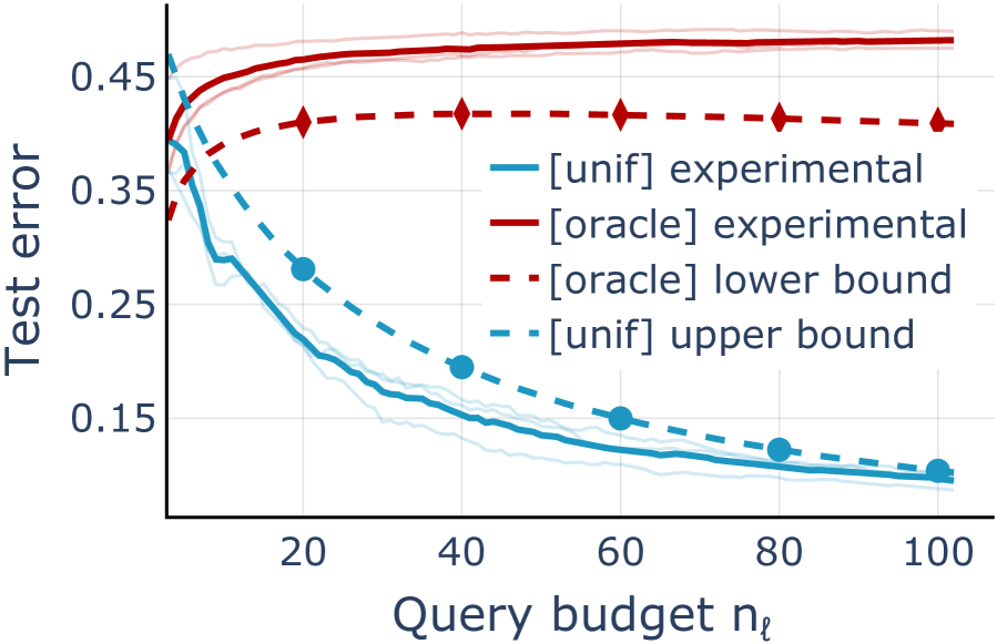
(a) Test error gap vs query budget

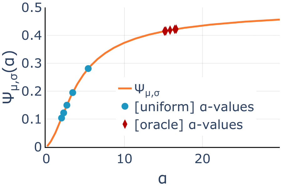
(b) $\Psi_{\mu,\sigma}(\alpha)$

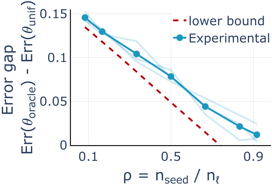
(c) Test error gap vs $\rho$

Figure 6: For large $d/n_{\ell}$ the bounds of Theorem B.2 are close to tight. (a) The bounds in Theorem B.2 (dashed lines) show that M-AL leads to lower test error compared to uniform sampling. The lighter color lines correspond to one of $3$ runs with different draws of the seed set, while the solid line indicates their mean. (b) The function $\Psi_{\mu,\sigma}(\alpha)$ is monotonically increasing in $\alpha$. The markers show the $(\alpha,\Psi_{\mu,\sigma}(\alpha))$ values corresponding to the query budgets indicated in figure (a). (c) By the bound in Theorem 3.3 (dashed line), the error gap between M-AL and PL decreases as the proportion of seed samples grows.

Appendix E Synthetic experiments on the mixture of truncated Gaussians distribution

In this section, we give the experimental details to the synthetic experiments in Figures 3(a) and 3(b). Further, we show empirically that for large $d/n_{\ell}$ the theoretical bounds closely predict the experimental values. Lastly, we further empirically discuss the dependency on the distributional parameters $\sigma$ and $\mu$ of the truncated Gaussian mixture model for empirical margin-based sampling.

E.1 Experimental details to Figures 3(a) and 3(b)

In both Figures 3(a) and 3(b), we plot the theoretical upper and lower bounds of Theorem B.2 with $n_{u}=10^{5}$, $t=3$ and compute $\Psi_{\mu,\sigma}$ by integrating using scikit-learn’s function "dblquad".

In Figure 3(a), we set $d=1000$, $\mu=2$, $\sigma=2$, $n_{\text{seed}}=10$ and vary $n_{\ell}$ from $n_{\text{seed}}$ to $1000$. On the other hand, in Figure 3(b) we set $d=1000$, $\sigma=2$ and vary the mean-parameter $\mu$ in $\{1,2,3\}$ and the seed set size $n_{\text{seed}}$ in $[1,...,n_{\ell}]$.

E.2 Verifying the bounds in Theorem B.2 on synthetic data

We now experimentally confirm the bounds in Theorem B.2. Recall that for large $d/n_{\ell}$, the bounds on $\tilde{\gamma}$ of Lemma C.1 are tight. Therefore we consider two settings where $d/n_{\ell}$ is large.

First, in Figure 3(a), we set $d=3k$, $n_{u}=10^{5}$, $\sigma=2$ and $\mu=3$. Then we vary $n_{\ell}$ from $n_{\text{seed}}$ to $100$. We plot the results of $3$ independent experiments for each setting along with the theoretical lower and upper bounds given in Theorem B.2. Observe that the theoretical bounds closely predict both the test error of passive learning as well as the test error of oracle M-AL.

Further, for completeness, in Figure 6(b) we also plot the function $\Psi_{\mu,\sigma}$ with corresponding $\alpha$-values from the setting in Figure 3(a). Observe that for small $\alpha$ the function $\Psi_{\mu,\sigma}$ increases fast.

Lastly, in Figure 6(c), we set $d=10k$,$n_{u}=10^{5}$, $\mu=0$, $\sigma=3$, $n_{\ell}=60$ and vary $n_{\text{seed}}$ from $5$ to $55$. Observe that the theoretical bound closely predicts the test error gap. Moreover, observe that the test error gap monotonically decreases in $\rho$ both experimentally and according to the theoretical bound.

Logistic regression implementation.

In all synthetic experiments, we use the SGDClassifier of the Scikit-learn library [31] with the following settings: we set the learning rate to be a constant of $10^{-4}$ and train for at least $10^{4}$ epochs without regularization. Moreover, we set the tolerance parameter to $10^{-5}$ and the maximum number of epochs to $10^{6}$. In all experiments, we consider regular margin-based sampling as defined in Algorithm 1.

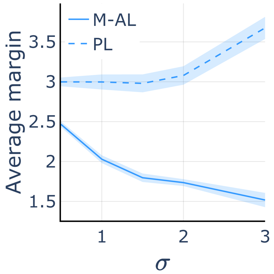
(a) Average margin in $\sigma$

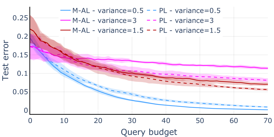
(b) Test error for varying $\sigma$

Figure 7: (a) M-AL collects labeled sets with a smaller average margin in the signal component as $\sigma$ increases. (b) As the average margin of a set acquired via M-AL is smaller for increasing $\sigma$, the test error deteriorates, as predicted by Lemma B.7. The test error of M-AL can even be larger than that of PL, for large enough $\sigma$. We use $d=1000$, $\mu=3$ and $n_{u}=10^{5}$ for all the experiments in this figure. The shaded areas indicate one standard deviation bands around the mean error, computed over 5 random draws of the seed set.

E.3 Dependence on the standard deviation $\sigma$ and seed size $n_{\text{seed}}$ for regular margin-based sampling

For completeness, we illustrate the dependence on the variance and the seed size of regular margin-based sampling with following experiments. To simulate realistic settings, we set $d=1000$, $n_{u}=10^{5}$, $n_{\text{seed}}=10$, $\sigma=3$ and $\mu=3$.

First, we perform a set of experiments to analyze the dependence on the variance $\sigma$ and to also confirm to main intuition empirically. We compute the average distance to the decision boundary of the ground truth $\theta^{\star}$ of a labeled set acquired via M-AL and PL. Indeed, in Figure 7(a) we see that the average margin of M-AL decreases with increasing $\sigma$. Moreover, we note that M-AL indeed queries points close to the optimal decision boundary. In Figure 7(b) we observe that, as predicted by Lemma B.7, the decrease of the average margin gap is directly correlated with an increase of the error gap between M-AL and PL. Hence, our main intuition is also here empirically verifiable: M-AL queries points relatively close to the ground truth, which causes in high dimensions the max-$\ell_{2}$-margin classifier to rely more on the non-signal components to classify the training data.

Secondly, we perform a set of experiments to an analyze the dependence on the seed size $n_{\text{seed}}$. In Figure 8, we see that the test error gap between M-AL and PL closes slowly for an increasing seed size. However, we note that the gap remains non-zero for all seed sizes up to $d/4$.

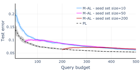
Figure 8: We set $d=1000$, $\mu=3$ and $n_{u}=10^{5}$. The shaded areas indicate one standard deviation bands around the mean error, computed over 5 random draws of the seed set. Observe that for increasing seed size the gap between M-AL and PL closes, but does not vanish. Note that we study the high-dimensional regime and hence only consider seed sizes up to $d/4$. Therefore, seed size larger than $d$ may fully close the test error gap between AL and PL.

Appendix F Experiment details for tabular data

F.1 Datasets

To assess how suitable margin-based sampling is for high-dimensional data, we conduct experiments on a wide variety of real-world datasets. We select datasets from OpenML [44] and from the UCI data repository [9] according to a number of criteria. In particular, we focus on datasets for binary classification that are high-dimensional ($d>100$) and which have enough samples that can serve as the unlabeled set ($n_{u}>\max(1000,2d)$). We do not consider text or image datasets where the features are sequences of characters or raw pixels as estimators other than linear models are better suited for these data modalities (e.g. CNNs, transformers etc). Instead we want to analyze M-AL in a simple setting and thus focus on datasets that are (approximately) linearly separable. Moreover, we discard datasets that have missing values. Finally, we are left with $15$ datasets that cover a broad range of applications from finance and ecology to chemistry and histology. We provide more details about the selected datasets in Appendix F.1.

To disentangle the effect of high-dimensionality from other factors such as class imbalance, we subsample uniformly at random the examples of the majority class, in order to balance the two classes. In addition, to ensure that the data is noiseless, we fit a linear classifier on the entire dataset, and remove the samples that are not interpolated by the linear estimator. This noiseless setting is advantageous for active learning, since we are guaranteed to not waste the limited labeling budget on noisy samples. However, as we show later, even in this favorable scenario, the performance of M-AL suffers in high-dimensions. For completeness, we also compare M-AL and PL on the original, uncurated datasets in Appendix G.1 and observe similar trends as in this section.

Dataset name	$d$	Training set size	Test set size	Majority/minority ratio	Linear classif. training error
a9a	123	39074	9768	3.17	0.1789
vehicleNorm	100	78823	19705	1.00	0.1415
nomao	118	27572	6893	2.50	0.0531
santander	200	160000	40000	8.95	0.2188
webdata_wXa	123	29580	7394	3.16	0.1813
sylva_prior	108	11516	2879	15.24	0.0011
real-sim	20958	57848	14461	2.25	0.0027
riccardo	4296	16000	4000	3.00	0.0007
guillermo	4296	16000	4000	1.49	0.2536
jasmine	144	2388	596	1.00	0.1867
madeline	259	2512	628	1.01	0.3405
philippine	308	4666	1166	1.00	0.2445
christine	1636	4335	1083	1.00	0.1408
musk	166	5279	1319	5.48	0.0438
epsilon	2000	48000	12000	1.00	0.0947

Table 1: Some characteristics of the uncurated datasets considered in our experimental study.

More dataset statistics.

Table 1 summarizes some important characteristics of the datasets. The datasets span a wide range of applications (e.g. ecology, finance, chemistry, histology etc). All datasets are high-dimensional ($d\geq 100$) and have sufficiently many training samples that will serve as the unlabeled set. The test error is computed on a holdout set, whose size we report in Table 1. We also present the class-imbalance of the original, uncurated datasets and the training error of a linear classifier trained on the entire dataset, which indicates the degree of linear separability of the data.

F.2 Methodology

We split each dataset in a test set and a training set. The covariates of the training samples constitute the unlabeled set. We assume that the labels are known for a small seed set of size $n_{\text{seed}}=6$ (see Appendix G.7 for experiments with larger seed sets). For each experiment and dataset, we repeat the draw of the seed set 10 or 100 times, depending on the experiment.

For illustration purposes, we set the labeling budget to be equal to a quarter of the number of dimensions. We query one point at a time and select the sample whose label we want to acquire either via uniform sampling (i.e. passive learning) or using margin-based sampling (i.e. active learning).

We use L-BFGS [26] to train linear classifiers by minimizing the logistic loss on the labeled dataset. In Appendix G.6 we show that the same high-dimensional phenomenon occurs when using $\ell_{1}$- or $\ell_{2}$-regularized classifiers.

Appendix G Additional experiments on tabular data

G.1 Experiments on uncurated data

For completeness, in this section we provide experiments on the original, uncurated datasets. We distinguish two scenarios: 1) balanced data, but not necessarily linearly separable; and 2) possibly imbalanced and not linearly separable data. In both cases, we use the same methodology described in Section 4 to plot the probability (over draws of the seed set) that the error with PL is lower than with M-AL and the losses/gains of M-AL compared to PL.

Balanced, but non-linearly separable data.

As indicated in Appendix F.1, not all datasets are originally linearly separable. For clarity, in the experiments in the main text we curate the data such that a linear classifier can achieve vanishing training error. This is provides a clean test bed for comparing margin-based and uniform sampling in high-dimensions.

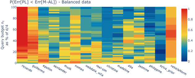
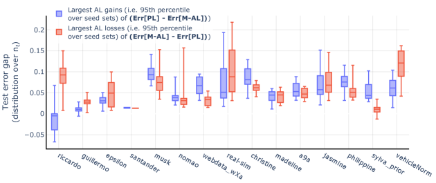
Figure 9: Top: The probability that the test error is lower with PL than with M-AL, over $10$ draws of the seed set. Data is class-balanced, but potentially not linearly separable. Bottom: For the range of budgets where M-AL does poorly with high probability, its sporadic gains over PL are generally similar or lower than the losses it can incur in terms of increased test error. Data is class-balanced, but potentially not linearly separable.

In Figure 9 we keep the datasets class-balanced, but allow them to be potentially not linearly separable. We observe similar trends as the ones illustrated in Figure 4 for the noiseless versions of the datasets.

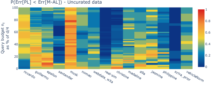
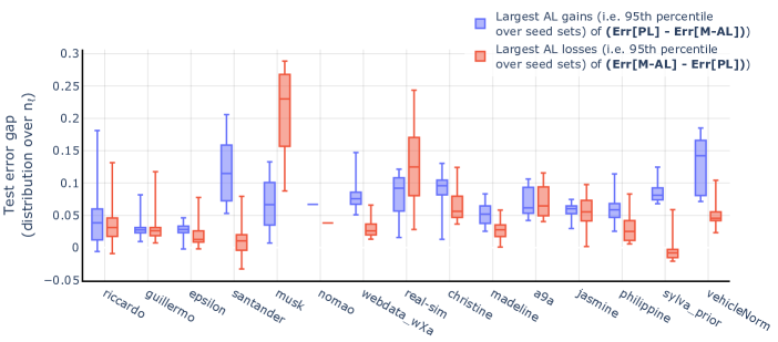
Figure 10: Top: The probability that the test error is lower with PL than with M-AL, over $10$ draws of the seed set. Data is potentially class-imbalanced and not linearly separable. Bottom: For the range of budgets where M-AL does poorly with high probability, its sporadic gains over PL are generally similar or lower than the losses it can incur in terms of increased test error.

Imbalanced and non-linearly separable data.

Margin-based sampling brings about surprising benefits when applied on high-dimensional imbalanced data. In particular, Figure 10 shows that for a broad range of query budgets margin-based sampling leads to better test error than uniform sampling. For these experiments we did not alter the original datasets in any way, and kept all the training samples.

These results reveal a perhaps unexpected phenomenon. When the unlabeled data is imbalanced (see Appendix F.1 for the exact imbalance ratio of each dataset), M-AL tends to achieve better predictive performance compared to passive learning. This phenomenon has also been previously observed by ertekin [11].

G.2 Uniform sampling versus oracle margin-based sampling

In this section we provide the counterpart of Figure 4, but now we use the distance to the Bayes optimal decision boundary for the active learning algorithm. Recall that for oracle M-AL we first train a classifier on the entire labeled dataset (this estimator will act as a stand-in for the Bayes optimal predictor). Then we use the distance to the decision boundary determined by this approximation of the Bayes optimal classifier to select points to query.

Figure 11 reveals that the gap between M-AL and PL is even more significant when using the oracle margin, which is in line with the intuition provided in Section 3. Oracle margin-based sampling will select samples close to the Bayes optimal decision boundary (i.e. the yellow points in Figure 3(c)). Hence, the decision boundary of the classifier trained on the labeled set collected with active learning will be tilted compared to the optimal predictor, as long as the query budget is significantly smaller than the dimensionality.

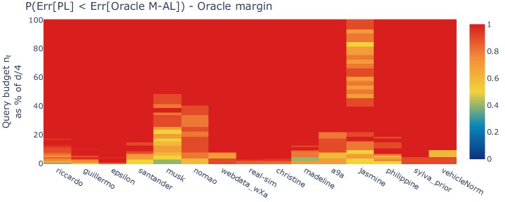
Figure 11: The probability that the test error is lower with PL than with oracle M-AL, over $10$ draws of the seed set. Oracle M-AL performs consistently worse than PL (warm-colored regions).

G.3 Test error at different query budgets – more datasets

We compare the test error of PL and M-AL, similar to Figure 1, but for more real-world datasets. For margin-based sampling, we use both the oracle margin and the margin of $f(\cdot;\hat{\theta})$ as shown in Algorithm 1. Figure 12 show that oracle M-AL consistently leads to larger test error compared to passive learning on all datasets. In addition, using the distance to the decision boundary determined by the max-$\ell_{2}$-margin classifier also leads to worse prediction performance, in particular on the high-dimensional datasets and for small query budgets. For illustration and computational purposes, we limit the query budget to $\min(3000,d/4)$.

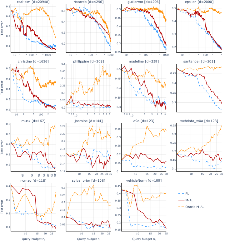
Figure 12: The test error using M-AL (with or without using the oracle margin) is often higher than what is achieved with uniform sampling, for all the datasets that we consider.

G.4 Another perspective on Figure 4

In Figure 4-Top we provide an overview of the gap that exists between M-AL and PL in high-dimensions. Here, we provide a more detailed perspective of the same evaluation metric. Each panel in Figure 13 corresponds to one column in Figure 4. The horizontal dashed line indicates the $50\%$ threshold at which the event that M-AL performs better is equally likely to its complement. Notice that in all figures the solid line starts at $0$, since before any queries are made, both uniform sampling and margin-based sampling yield the same test error, namely the error of the max-$\ell_{2}$-margin classifier trained on the seed set.

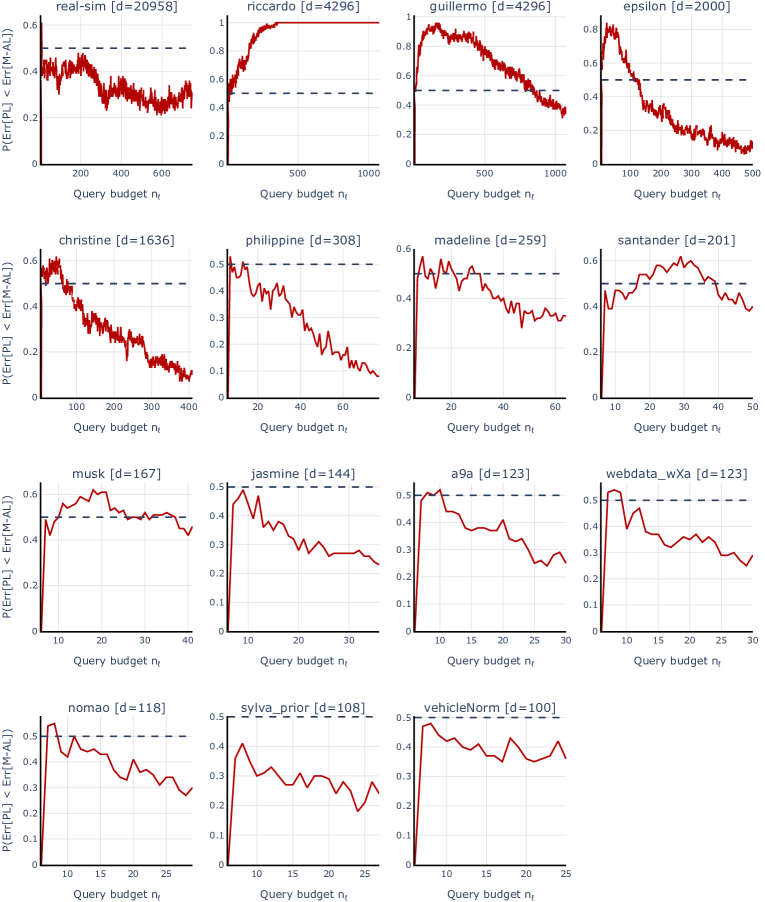
Figure 13: The probability that M-AL performs worse than PL at different query budgets. The empirical probability is computed over $100$ draws of the initial seed set.

We note that the spikes in the lines in Figure 13 come from the fact that for different seed sets, M-AL may start to underperform at different iterations. Hence, aggregating over several seed sets leads to the non-smooth lines in the figure.

In addition, in Figure 14 we summarize each of the panels in Figure 13 in a box plot that offers yet another perspective on this experiment. Notably, the boxes are fairly concentrated for all datasets, confirming that the gap between the test error with uniform and margin-based sampling stays roughly the same for any query budget $n_{q}\in\{n_{\text{seed}},...,d/4\}$. Note that here the probability is over the draws of the seed set, and the box plots show percentiles of the distribution over query budgets for each dataset.

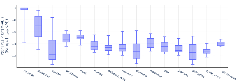
Figure 14: Box plot of the distribution of P(Err[PL] $<$ Err[AL]) over query budgets $n_{q}\in\{n_{\text{seed}},...,d/4\}$.

For these experiments we use the distance to the decision boundary determined by the estimator $f(\cdot;\hat{\theta})$ as shown in Algorithm 1. In Figure 4-Bottom we show the largest gains and losses of M-AL for query budgets $n_{q}\in\{n_{\text{seed}},...,n_{\text{transition}}\}$, where $n_{\text{transition}}$ is defined as the budget after which M-AL is always better than PL with probability at least $50\%$. In other words, one can read $n_{\text{transition}}$ off Figure 13 as the leftmost point on the horizontal axis for which the solid line intersects the horizontal dashed line. For datasets that never intersect the $50\%$ dashed line, we take $n_{\text{transition}}=d/4$ conservatively. This is more advantageous for M-AL, as larger query budgets tend to lead to larger gains over PL.

G.5 Fraction of budgets for which active learning underperforms

An alternative to using the metric illustrated in Figure 4-Top and in Appendix G.4 is to instead compute the fraction of the query budgets for which active learning performs worse than passive learning. In Figure 15 we present this evaluation metric for all the datasets that we consider. The box plot indicates the distribution over $100$ draws of the initial seed set. For all datasets and with high probability over the draws of the seed data M-AL underperforms on a large fraction of the query budgets between $n_{\text{seed}}$ and $d/4$.

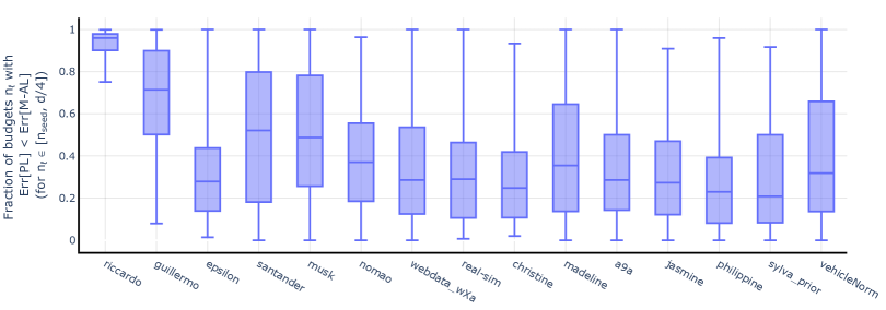
Figure 15: Fraction of the query budgets between $n_{\text{seed}}$ and $d/4$ for which the error with M-AL is worse than with PL. The box plot indicates the distribution over $100$ draws of the seed set (median, lower and upper quartiles).

Note that the fences of the box plots that almost cover the entire $[0,1]$ range are a consequence of having a large number of runs (i.e. $100$). The whiskers indicate the minimum and maximum values and they will be more extreme, the larger the set over which we take the minimum/maximum is.

G.6 Experiments with regularized estimators

The failure case of margin-based active learning that we discuss in this paper is not limited to the situation when we use interpolating estimators. Indeed, as we show here, even regularization in the form of an $\ell_{2}$ or $\ell_{1}$ penalty still leads to classifiers with high test error when the data is collected using margin-based sampling.

We not that, in what follows, a small coefficient $C$ corresponds to stronger regularization, since we employ the scikit-learn [31] implementation of penalized logistic regression. Therefore $C\to 0$ implies the predictive error term in the loss is ignored, while $C\to\infty$ leads to no regularization (note that unless otherwise specified, all results throughout the paper are reported for the unregularized max-$\ell_{2}$-margin classifier).

Figures 16 and 17 indicate that for strong enough regularization, the gap between the test error of M-AL and PL vanishes. This outcome is expected since stronger regularization leads to a poorer fit of the data, and hence, classifiers trained on different data sets (e.g. one collected with M-AL and another collected with PL) will tend to be similar. The downside of increasing regularization is, of course, worse predictive performance. For instance, for an $\ell_{1}$ penalty and a coefficient of $0.01$, the test error is close to that of a random predictor (i.e. $50\%$) an all datasets for both uniform and margin-based sampling. For moderate regularization, there continue to exist broad ranges of query budgets for which M-AL underperforms compared to passive learning.

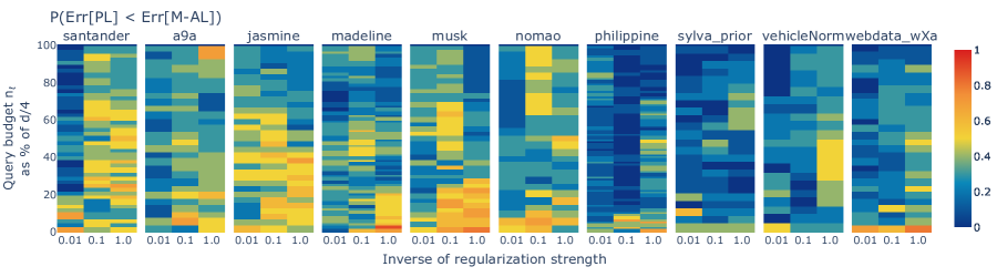
Figure 16: The probability that the test error is lower with PL than with M-AL, over $10$ draws of the seed set. We use an $\ell_{2}$-regularized classifier for both prediction and margin-based sampling. Note that smaller values along the x-axis correspond to stronger regularization. If we regularize too much (e.g. for a coefficient of $0.01$), the prediction error is poor for both PL and M-AL, which explains the light-colored regions.

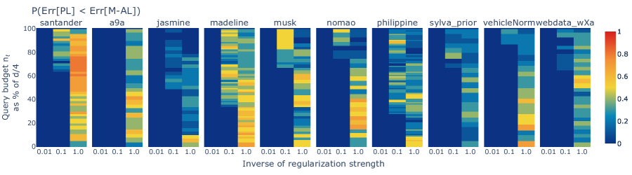
Figure 17: The probability that the test error is lower with PL than with M-AL, over $10$ draws of the seed set. We use an $\ell_{1}$-regularized classifier for both prediction and margin-based sampling. Note that smaller values along the x-axis correspond to stronger regularization. If we regularize too much (e.g. for a coefficient of $0.01$), the prediction error is poor for both PL and M-AL, which explains the light-colored regions.

G.7 Experiments with different seed set sizes

Our theory predicts that for a fixed labeling budget and an increasing see set size, the gap between the error with margin-based sampling and uniform sampling vanishes. We verify this insight experimentally in Figures 18 and 19. Our empirical findings confirm the trend predicted by our theory: margin-based sampling leads to better performance for large seed set sizes, but underperforms for small seed sets.

Perhaps surprisingly, the same trend occurs even for oracle M-AL. This is noteworthy, since prior work suggests that the failure of margin-based sampling for small seed set sizes is due to the usage of a meaningless score: the distance to a potentially very incorrect decision boundary obtained after training a predictor on the small seed set. Instead, our results show that margin-based sampling fails even when using the Bayes optimal predictor, which highlights a novel failure case of this sampling strategy.

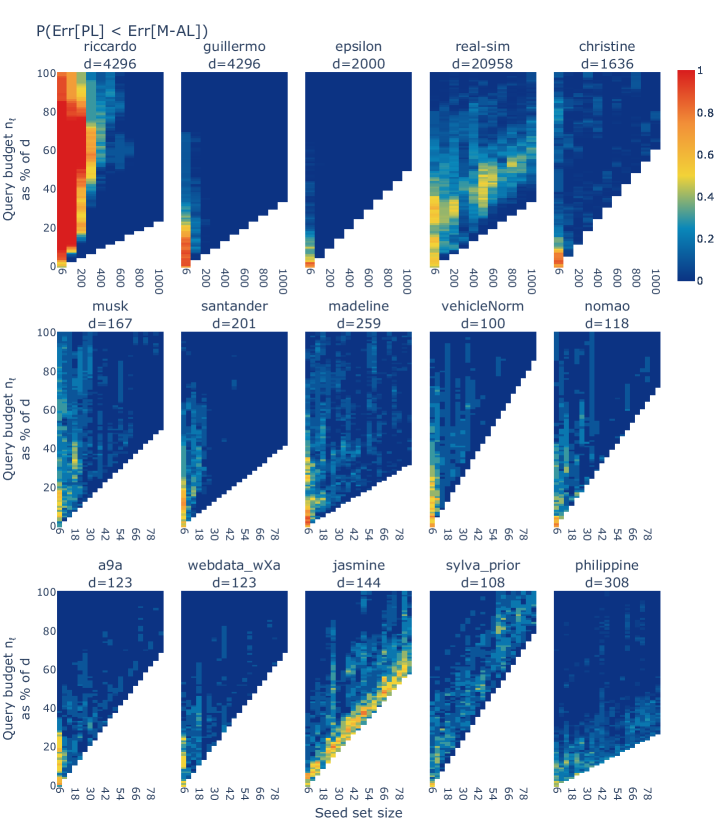
Figure 18: As predicted by our theory, increasing the seed size leads to improved performance when using M-AL to acquire new labeled samples.

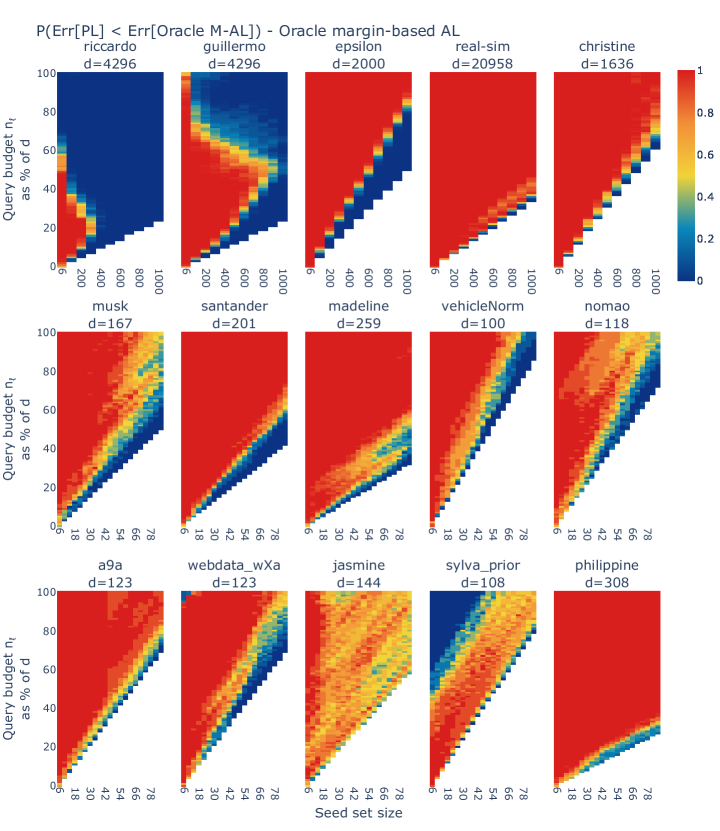
Figure 19: Surprisingly, increasing the seed set size also benefits oracle M-AL. This trend is not predicted by prior work and underlines a novel failure case of M-AL for high-dimensional data.

G.8 Combining informativeness and representativeness

In this section we provide evidence that the shortcoming of margin-based sampling that we identify in this paper also extends to other active learning strategies that try to balance exploration and exploitation. In particular, we focus on an ${\epsilon}$-greedy strategy which selects points using margin-based sampling with probability $1-{\epsilon}$, and samples points uniformly at random with probability ${\epsilon}$. Hence, this approach combines selecting informative samples via M-AL with collecting a labeled set that is representative of the training distribution. This strategy resembles the works of brinker03 [5, 20, 48, 15, 39].

First, we note that for oracle M-AL, the ${\epsilon}$-greedy strategy is equivalent to simply selecting a larger uniform seed set, since the queries are independent of each other when we use the oracle margin. Therefore, for a fixed query budget $n_{\ell}$, the ${\epsilon}$-greedy strategy with oracle M-AL is identical to regular oracle M-AL sampling where $n_{\text{seed}}={\epsilon}\cdot n_{\ell}$. We conclude that the results in Section G.7, and more specifically Figure 19, show that the ${\epsilon}$-greedy strategy performs worse than uniform sampling when using oracle M-AL.

Finally, we check whether the ${\epsilon}$-greedy strategy using the margin of the empirical predictor $\hat{\theta}$ is also detrimental compared to passive learning. We notice in Figure 20 that for different values of ${\epsilon}$, active learning continues to perform worse than passive learning. Varying ${\epsilon}$ between $0$ and $1$ effectively interpolates between vanilla margin-based sampling and uniform sampling.

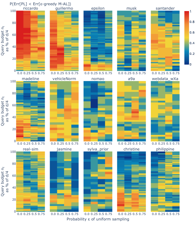
Figure 20: The probability that the test error is lower with uniform sampling than with an ${\epsilon}$-greedy sampling approach, over $10$ draws of the seed set. The active learning strategy performs margin-based sampling, with probability $1-{\epsilon}$ and samples uniformly at random with probability ${\epsilon}$.

G.9 Coreset-based active learning

In this section we investigate whether the coreset-based sampling strategy proposed in sener18 [37] can be a viable alternative to margin-based sampling in low-sample regimes. We follow the same active learning methodology as described in Section 4, but use the greedy algorithm from sener18 [37] to select queries. We use the Euclidean distance for our experiments.

Figure 21 shows that for a large fraction of query budgets, coreset-based active learning outperforms M-AL with high probability (warm-colored areas). However, for some datasets (e.g. vehicleNorm, a9a, philippine), coreset-based sampling can still lead to larger error than passive learning, as illustrated in Figure 22. We hypothesize that this behavior is due to not constraining the queried points to lie far from the Bayes optimal decision boundary. Hence, the high-dimensional phenomenon that we describe in Section 3 still occurs.

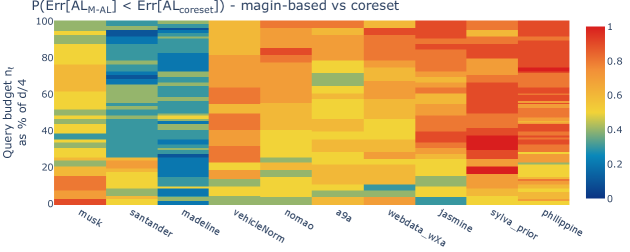
Figure 21: Coreset AL [37] sometimes outperforms M-AL with high probability (blue regions).

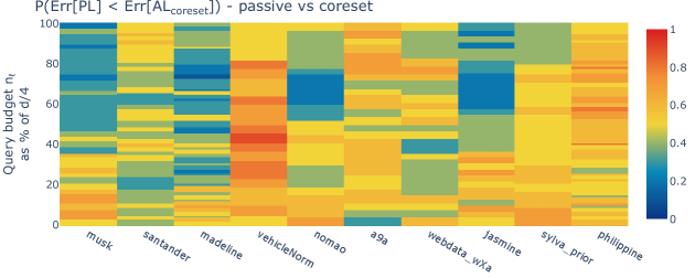
Figure 22: On some datasets (e.g. vehicleNorm), PL outperforms coreset-based active learning in the low-sample regime.

Appendix H Experiments on image datasets

In this section we describe our experiments on image datasets in which we explore the limitations of margin-based sampling for low query budgets.

H.1 Experiment details

We consider three standard image datasets: CIFAR10 [23], CIFAR100 [23], SVHN [30]. In addition to these, we also run experiments on a binary classification task for medical images (PCAM [45]) and on a 10-class task on satellite images (EuroSAT [19]). For prediction and for the sampling strategy we use ResNet18 networks [18] and start from weights pretrained on ImageNet. The sampling strategy consists in selecting the unlabeled point on which the trained prediction model has lowest confidence, as indicated by the softmax outputs. We note that this uncertainty-based strategy is closely related to the margin-based strategy that we use in binary classification problems.

To get a good estimate of the Bayes optimal classifier for Oracle M-AL, we train on the entire labeled training set for each dataset until the training error reaches $0$. We consider batch active learning, as usual in the context of deep learning, and set the batch size to $20$ (experiments with larger batch sizes lead to similar results). For each dataset, we start from an initial seed set of $100$ labeled examples and perform $50$ queries. Hence, the largest query budget that we consider is of $1100$ labeled samples. After each query step, we fine-tune the ResNet18 model for $20$ epochs, and achieve $0$ training error. For fine-tuning we use SGD with a learning rate of $0.001$ and momentum coefficient of $0.9$.

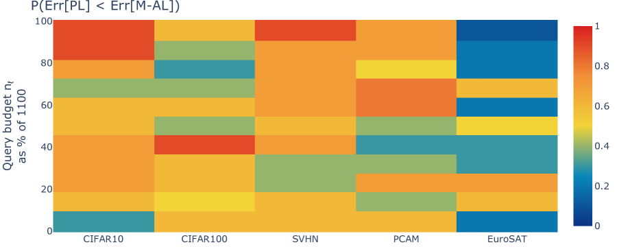
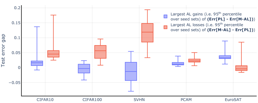
Figure 23: Top: Probability that the test error is lower with PL versus M-AL, over 10 different random seeds. PL outperforms M-AL, for a significant fraction of the query budgets (i.e. warm-colored regions). Bottom: The sporadic gains of M-AL over PL are generally similar or lower than the losses it can incur in terms of increased test error (negative values indicate that PL is always better than AL).

Summary of results.

As illustrated in Figure 23, AL leads to significantly larger test error compared to PL. This phenomenon persists even when we use the Bayes optimal classifier (Figure 24). Moreover, the gains that the active learning strategy can produce, are often dominated by the losses that it can incur. Note that for Figure 23-Bottom and Figure 24-Bottom we take $n_{\text{transition}}=1100$, namely the maximum query budget $n_{\ell}$ that we consider.

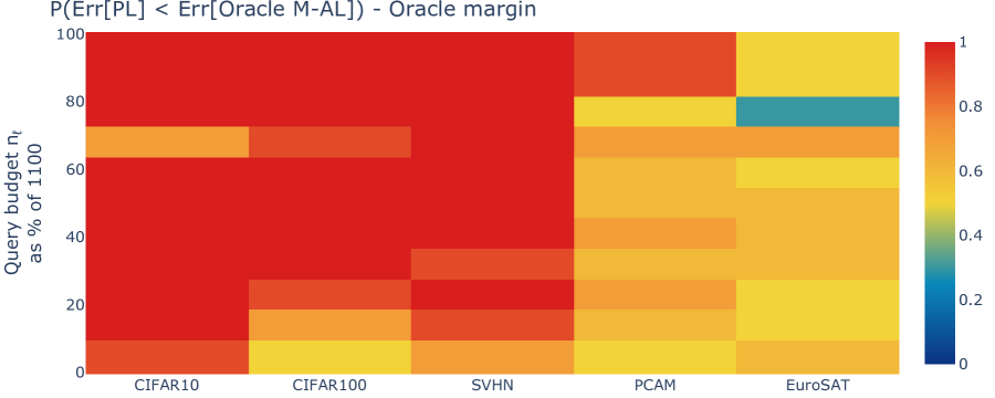
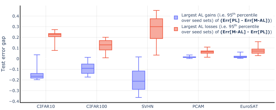
Figure 24: Same experiment as in Figure 23, but this time using oracle M-AL. Similar to the logistic regression experiments, M-AL leads to even worse error when using the Bayes optimal classifier for sampling, as predicted by our theory.

References

- [1] M.-F. Balcan, A. Broder, and T. Zhang. Margin based active learning. In N. H. Bshouty and C. Gentile, editors, Learning Theory, pages 35–50, 2007.
- [2] P. L. Bartlett, P. M. Long, G. Lugosi, and A. Tsigler. Benign overfitting in linear regression. Proceedings of the National Academy of Sciences, pages 30063–30070, 2020.
- [3] A. Beygelzimer, D. J. Hsu, J. Langford, and T. Zhang. Agnostic active learning without constraints. In Advances in Neural Information Processing Systems, 2010.
- [4] N. Bouguila and W. Fan. Mixture Models and Applications. Springer, 2019.
- [5] K. Brinker. Incorporating diversity in active learning with support vector machines. In Proceedings of the 20th International Conference on Machine Learning, 2003.
- [6] K. Chaudhuri, S. M. Kakade, P. Netrapalli, and S. Sanghavi. Convergence rates of active learning for maximum likelihood estimation. Proceedings in Advances in Neural Information Processing Systems 28, 2015.
- [7] D. Cohn, R. Ladner, and A. Waibel. Improving generalization with active learning. In Machine Learning, 1994.
- [8] K. Donhauser, A. Tifrea, M. Aerni, R. Heckel, and F. Yang. Interpolation can hurt robust generalization even when there is no noise. In Proceedings in Advances in Neural Information Processing Systems 34, 2021.
- [9] D. Dua and C. Graff. UCI machine learning repository, 2017.
- [10] M. Ducoffe and F. Precioso. Adversarial active learning for deep networks: a margin based approach. arXiv preprint arXiv:1802.09841, 2018.
- [11] S. Ertekin, J. Huang, L. Bottou, and L. Giles. Learning on the border: Active learning in imbalanced data classification. In Proceedings of the Sixteenth ACM Conference on Conference on Information and Knowledge Management, 2007.
- [12] S. Farquhar, Y. Gal, and T. Rainforth. On statistical bias in active learning: How and when to fix it. In Proceedings of the 9th International Conference on Learning Representations, 2021.
- [13] S. Frei, D. Zou, Z. Chen, and Q. Gu. Self-training converts weak learners to strong learners in mixture models. In Proceedings of The 25th International Conference on Artificial Intelligence and Statistics, 2022.
- [14] Y. Gal, R. Islam, and Z. Ghahramani. Deep Bayesian active learning with image data. In Proceedings of the 34th International Conference on Machine Learning, 2017.
- [15] D. Gissin and S. Shalev-Shwartz. Discriminative active learning. arXiv preprint arXiv:1907.06347, 2019.
- [16] G. Hacohen, A. Dekel, and D. Weinshall. Active learning on a budget: Opposite strategies suit high and low budgets. arXiv preprint arXiv:2202.02794, 2022.
- [17] S. Hanneke. A Statistical Theory of Active Learning. 2013.
- [18] K. He, X. Zhang, S. Ren, and J. Sun. Deep residual learning for image recognition. In Proceedings of the IEEE Conference on Computer Vision and Pattern Recognition (CVPR), 2016.
- [19] P. Helber, B. Bischke, A. Dengel, and D. Borth. Eurosat: A novel dataset and deep learning benchmark for land use and land cover classification. arXiv preprint arXiv:1709.00029, 2017.
- [20] S.-J. Huang, R. Jin, and Z.-H. Zhou. Active learning by querying informative and representative examples. Proceedings in Advances in Neural Information Processing Systems 27, 2014.
- [21] A. Javanmard and M. Soltanolkotabi. Precise statistical analysis of classification accuracies for adversarial training. arXiv preprint arXiv:2010.11213, 2020.
- [22] Z. Ji and M. Telgarsky. The implicit bias of gradient descent on nonseparable data. In Proceedings of the Conference on Learning Theory (COLT), 2019.
- [23] A. Krizhevsky. Learning multiple layers of features from tiny images. Technical report, 2009.
- [24] D. D. Lewis and W. A. Gale. A sequential algorithm for training text classifiers. In Proceedings of the international ACM SIGIR Conference on Research and Development in Information Retrieval, 1994.
- [25] M. Li, M. Soltanolkotabi, and S. Oymak. Gradient descent with early stopping is provably robust to label noise for overparameterized neural networks. In Proceedings of the Twenty Third International Conference on Artificial Intelligence and Statistics, 2020.
- [26] D. C. Liu and J. Nocedal. On the limited memory BFGS method for large scale optimization. Math. Programming, 45(3, (Ser. B)), 1989.
- [27] C. Mayer and R. Timofte. Adversarial sampling for active learning. In Proceedings of the IEEE/CVF Winter Conference on Applications of Computer Vision (WACV), 2020.
- [28] S. Mussmann and P. Liang. On the relationship between data efficiency and error for uncertainty sampling. In Proceedings of the 34th International Conference on Machine Learning, 2018.
- [29] V. Muthukumar, A. Narang, V. Subramanian, M. Belkin, D. Hsu, and A. Sahai. Classification vs regression in overparameterized regimes: Does the loss function matter? The Journal of Machine Learning Research, pages 10104–10172, 2021.
- [30] Y. Netzer, T. Wang, A. Coates, A. Bissacco, B. Wu, and A. Y. Ng. Reading digits in natural images with unsupervised feature learning. In NIPS Workshop on Deep Learning and Unsupervised Feature Learning, 2011.
- [31] F. Pedregosa, G. Varoquaux, A. Gramfort, V. Michel, B. Thirion, O. Grisel, M. Blondel, P. Prettenhofer, R. Weiss, V. Dubourg, J. Vanderplas, A. Passos, D. Cournapeau, M. Brucher, M. Perrot, and E. Duchesnay. Scikit-learn: Machine learning in Python. Journal of Machine Learning Research, 2011.
- [32] J. C. Platt. Probabilistic outputs for support vector machines and comparisons to regularized likelihood methods. In Advances in Large Margin Classifiers, 1999.
- [33] T. Scheffer and S. Wrobel. Active learning of partially Hidden Markov Models. In In Proceedings of the ECML/PKDD Workshop on Instance Selection, 2001.
- [34] A. I. Schein and L. H. Ungar. Active learning for logistic regression: An evaluation. Machine Learning, 2007.
- [35] G. Schohn and D. Cohn. Less is more: Active learning with support vector machines. In Proceedings of the 17th International Conference on Machine Learning, 2000.
- [36] B. Scholkopf, D. Janzing, J. Peters, E. Sgouritsa, K. Zhang, and J. Mooij. On causal and anticausal learning. In Proceedings of the 29th International Conference on Machine Learning, 2012.
- [37] O. Sener and S. Savarese. Active learning for convolutional neural networks: A core-set approach. In Proceedings of the 6th International Conference on Learning Representations, 2018.
- [38] B. Settles. Active learning literature survey. 2009.
- [39] C. Shui, F. Zhou, C. Gagné, and B. Wang. Deep active learning: Unified and principled method for query and training. In Proceedings of the Twenty Third International Conference on Artificial Intelligence and Statistics, 2020.
- [40] B. Sorscher, R. Geirhos, S. Shekhar, S. Ganguli, and A. S. Morcos. Beyond neural scaling laws: beating power law scaling via data pruning. In Proceedings in Advances in Neural Information Processing Systems 36, 2022.
- [41] D. Soudry, E. Hoffer, M. S. Nacson, S. Gunasekar, and N. Srebro. The implicit bias of gradient descent on separable data. Journal of Machine Learning Research, 2018.
- [42] S. Tong and D. Koller. Support vector machine active learning with applications to text classification. Journal of Machine Learning Research, 2001.
- [43] D. Tsipras, S. Santurkar, L. Engstrom, A. Turner, and A. Madry. Robustness may be at odds with accuracy. In International Conference on Learning Representations, 2019.
- [44] J. Vanschoren, J. N. van Rijn, B. Bischl, and L. Torgo. OpenML: networked science in machine learning. SIGKDD Explorations, 2013.
- [45] B. S. Veeling, J. Linmans, J. Winkens, T. Cohen, and M. Welling. Rotation equivariant CNNs for digital pathology. arXiv preprint arXiv:1806.03962, 2018.
- [46] R. Vershynin. Introduction to the non-asymptotic analysis of random matrices. arXiv preprint arXiv:1011.3027, 2010.
- [47] Y. Yang and M. Loog. A benchmark and comparison of active learning for logistic regression. Pattern Recognition, 2018.
- [48] Y. Yang, Z. Ma, F. Nie, X. Chang, and A. G. Hauptmann. Multi-class active learning by uncertainty sampling with diversity maximization. International Journal of Computer Vision, 2015.
- [49] C. Zhang. Efficient active learning of sparse halfspaces. In Proceedings of the 31st Conference On Learning Theory, pages 1856–1880, 2018.