Neural Representations Reveal Distinct Modes of Class Fitting in Residual Convolutional Networks

Abstract

We leverage probabilistic models of neural representations to investigate how residual networks fit classes. To this end, we estimate class-conditional density models for representations learned by deep ResNets. We then use these models to characterize distributions of representations across learned classes. Surprisingly, we find that classes in the investigated models are not fitted in an uniform way. On the contrary: we uncover two groups of classes that are fitted with markedly different distributions of representations. These distinct modes of class-fitting are evident only in the deeper layers of the investigated models, indicating that they are not related to low-level image features. We show that the uncovered structure in neural representations correlate with memorization of training examples and adversarial robustness. Finally, we compare class-conditional distributions of neural representations between memorized and typical examples. This allows us to uncover where in the network structure class labels arise for memorized and standard inputs.

Introduction

Neural networks are vastly over-parametrized models. This flexible parameter space makes it quite difficult to answer basic questions about internal representations learned by these models. For a long time it was not even clear whether two identical networks trained on the same task learn similar sets of representations. That said, the picture begin to change in recent years with the introduction of new tools to analyse internal representations in neural networks. First, Raghu et al. (2017) and Morcos, Raghu, and Bengio (2018) proposed canonical correlation analysis-based similarity measures for neural representations. Subsequently, Kornblith et al. (2019) proposed a kernel-based similarity score and found significant representational similarity between networks trained to solve closely related tasks. Machinery for analysis of neural representations was then extended by Jamroż, Kurdziel, and Opala (2020), who proposed a non-parametric density model for features learned by neural networks. They used this model to show that memorizing networks learn more complex representations than networks that can exploit patterns in data.

So far neural representations were studied from the perspective of features learned by network layers. In this work we extend this line of research to investigate class representations learned by neural networks. To this end, we estimate class-conditional distributions of neural representations and use them as proxies to the representations of classes learned by the network. This allows us to make several important contributions. First, we find that ResNets do not fit classes in an uniform way. On the contrary, we observe two distinct modes of class fitting evident in the deeper layers of these networks. We characterize class-conditional distributions of neural representations in the two groups of classes and propose a likely explanation for the observed differences. Next, we demonstrate that the uncovered structure in class representations translates to observable differences in memorization of input examples. To this end, we leverage tractable memorization measures recently proposed by Feldman and Zhang (2020). We also demonstrate that the two groups of classes differ in adversarial robustness. Finally, we leverage class-conditional distributions of neural representations to uncover where in the network structure classes are fit and to compare this process for memorized and typical inputs.

While this work focuses on convolutional residual networks, in the appendix we also report initial results for non-convolutional models with skip connections, namely Vision Transformers (Dosovitskiy et al. 2021) and MLP-Mixers (Tolstikhin et al. 2021). We provide the source code for the experiments, as well as our density and memorization estimates.

Probabilistic model for class representations

Our goal in this work is to characterize representations of classes in neural networks. While the class membership information is typically available for a large set of observations, namely the training set, combining it into representations of classes is a non-trivial task. The main hurdle here comes from the stochastic nature of neural representations. Specifically, a neural representation inferred for some input $\mathbf{x}$ can be seen as an outcome of sampling $\mathbf{x}$ from the data distribution. Clearly, a reasonable notion of a class representation should capture the outcome of this sampling. We therefore propose to use class-conditional distributions of inputs’ representations as proxies to neural representations of classes. Concretely, we fit tractable density models to sets of neural representations and then use these models to characterize distributions of representations in classes.

We capture the distributions of neural representations with the hierarchical Bayesian model that was recently used by Jamroż, Kurdziel, and Opala (2020) to investigate networks that fit random labels. Jamroż, Kurdziel, and Opala used this model to characterize representations of kernels in convolutional layers. A neural representation in their work was therefore defined as a vector of kernel responses over a fixed sequence of inputs, averaged across spatial dimensions. Our goal, however, is not to investigate features learned by convolutional kernels, but to characterize—in distributional settings—representations of inputs from the learned classes. We therefore adopt a different construction for neural representations. Specifically, in modern variable-resolution convolutional models input to the classification head is frequently constructed by global average pooling of the output feature maps. We follow a similar construction for representations of inputs in our class-conditional density models. In particular, consider a network layer $l$ with a sequence of convolutional kernels: $k^{l}_{1},k^{l}_{2},\ldots,k^{l}_{d}$—where $d$ is the layer width—and let $\mathbf{x}\in C$ be an input observation from class $C$. We construct the representation of $\mathbf{x}$ at layer $l$ as the vector of respective kernel activations averaged across spatial dimensions:

$$\begin{split}nn_{l}\left(\mathbf{x}\right)=&\left[\mathrm{avg\_pool}(k^{l}_{1}(\mathbf{x})),\mathrm{avg\_pool}(k^{l}_{2}(\mathbf{x})),\ldots,\right.\\ &\ \left.\mathrm{avg\_pool}(k^{l}_{d}(\mathbf{x}))\right].\end{split}$$ (1)

Activation vectors for all inputs $\mathbf{x}\in C$ collectively form a set of observations that is then explained with the density model. Because all input observations are sampled from $C$, the model estimates the class-conditional distribution for $C$.

Density model

The hierarchical Bayesian model used by Jamroż, Kurdziel, and Opala (2020) explains a set of observations $\mathbf{x}\in\mathcal{D}$—e.g. a set of neural representations of some network inputs—with a mixture of multivariate normal distributions with an unknown number of components:

$$\begin{split}\alpha&\sim Gamma(1,1),\\ G\mid\alpha&\sim DP(NIW(\bm{\theta}_{0}),\alpha),\\ \bm{\mu}_{k},\bm{\Sigma}_{k}&\sim G,\\ \bm{x}\mid\bm{\mu}_{k},\bm{\Sigma}_{k}&\sim\mathcal{N}(\bm{\mu}_{k},\bm{\Sigma}_{k}).\end{split}$$ (2)

The prior over component parameters is constructed as a Dirichlet Process ($DP)$ with Normal-Inverse-Wishart ($NIW$) base distribution. A mixture of this form is consistent in total variation for a large family of continuous distributions (Ghosal and Van der Vaart 2017) and admits an efficient collapsed Gibbs sampler (CGS) for the posterior over component parameters (Neal 2000). Shortly, CGS constructs a Markov chain over assignments of observations to components: $\left(\bm{c}_{1},\bm{c}_{2},\bm{c}_{3},\ldots\right)$. Under the model in Eq. (2), the conditional posterior predictive distribution $p(\bm{x^{*}}\mid\mathcal{D},\bm{c}_{t})$ over a new observation $\bm{x^{*}}$ given the set of assignments $\bm{c}_{t}$ has a closed-form solution (Jamroż, Kurdziel, and Opala 2020). This conditional predictive distribution can be leveraged to construct a tractable Monte Carlo approximation to the full posterior predictive distribution:

$$p(\bm{x^{*}}\mid\mathcal{D})\approx\frac{1}{n}\sum_{t=1}^{n}p(\bm{x^{*}}\mid\mathcal{D},\bm{c}_{t}).$$ (3)

The average here is taken over the assignments sampled by CGS, i.e. over the Markov chain steps.

The closed-form solution for the predictive distribution conditioned on component assignments $p(\bm{x^{*}}\mid\mathcal{D},\bm{c}_{t})$ gives a simple sampling strategy for the full posterior predictive: sample a component assignment $\bm{c}_{t}$ from the Markov chain and then sample $\bm{x^{*}}$ from the induced conditional distribution $p(\bm{x^{*}}\mid\mathcal{D},\bm{c}_{t})$. This sampling scheme can be used to compare the posterior predictive distribution with another distribution $q\left(\bm{x^{*}}\right)$ that has a tractable density. Specifically, the samples can be used to construct a Monte Carlo approximation to the relative entropy—or Kullback-Leibler (KL) divergence—from $q\left(\bm{x^{*}}\right)$ to $p(\bm{x^{*}}\mid\mathcal{D})$:

$$\begin{split}&D_{\mathrm{KL}}\left(p\left(\bm{x^{*}}\mid\mathcal{D}\right)\;\left|\right|\;q\left(\bm{x^{*}}\right)\right)=\\ &\quad=\operatorname*{\mathbb{E}}_{\bm{x^{*}}\sim p\left(\bm{x^{*}}\mid\mathcal{D}\right)}\left[\log p\left(\bm{x^{*}}\mid\mathcal{D}\right)-\log q\left(\bm{x^{*}}\right)\right]\\ &\quad\approx\frac{1}{nm}\sum_{t=1}^{n}\sum_{s=1}^{m}\left[\log p\left(\bm{x^{*}}_{st}\mid\mathcal{D},\bm{c}_{t}\right)-\log q\left(\bm{x^{*}}_{st}\right)\right],\end{split}$$ (4)

where $\bm{x^{*}}_{st}$ are sampled from $p\left(\bm{x^{*}}\mid\mathcal{D},\bm{c}_{t}\right)$. As proposed by Jamroż, Kurdziel, and Opala, the estimate in Eq. (4) can be used to quantify the complexity of neural representations. In this case the reference distribution $q\left(\bm{x^{*}}\right)$ is chosen to be the maximum entropy distribution that explains only the location and the scale of $\mathcal{D}$, i.e. the diagonal Gaussian with the mean and the variances estimated from $\mathcal{D}$.

In this work we use the divergence from the maximum entropy distribution to characterize the complexity of class-conditional distributions of neural representations. We also use Eq. (4) to compare posterior predictive distributions estimated for different classes. Specifically, let $p\left(\bm{x^{*}}\mid\mathcal{F}\right)$ be the posterior predictive distribution under model in Eq. (2) induced by a set of neural representations $\mathcal{F}$. Because the density in this posterior predictive is tractable (Eq. (3)), we can use Eq. (4) to estimate the KL divergence from $p\left(\bm{x^{*}}\mid\mathcal{F}\right)$ to $p(\bm{x^{*}}\mid\mathcal{D})$. To this end, we simply set the reference distribution $q\left(\bm{x^{*}}\right)$ to be the posterior predictive $p\left(\bm{x^{*}}\mid\mathcal{F}\right)$.

Standard CGS exhibits relatively slow mixing. To speed-up the estimation of predictive distributions, in this work we sample posterior parameters using a variant of this algorithm with blocked Gibbs sampling (Jensen, Kjærulff, and Kong 1995). See Appendix for more details.

Memorization in neural networks

Recently, Feldman (2020) proposed a theoretical framework that explains the role of input memorization when fitting a long-tailed data distribution, i.e. a population of input examples characterized by many infrequent components. They consider a case where some of the examples in an $n$-element train set come from sub-populations with frequency below $1/n$. Such examples are statistically indistinguishable from noise or mislabelled data. Consequently, their fitting requires memorization. Importantly, Feldman showed that memorization in these settings is in fact necessary to minimize the generalization error. They also proposed a measure for the degree of input memorization. Specifically, given a learning algorithm $\mathcal{A}$ and an example $\left(\mathbf{x},t\right)$, Feldman defines the degree of memorization of $\left(\mathbf{x},t\right)$ as the probability of predicting $t$ for input $\mathbf{x}$ when $\left(\mathbf{x},t\right)$ is observed during training, relative to the probability of the correct prediction when $\left(\mathbf{x},t\right)$ is absent from the training data. A score of $1.0$ therefore corresponds to an example that is memorized in every training run, whereas a score of $0.0$ corresponds to an example with no memorization. This definition assumes that $\mathcal{A}$ is a stochastic learning algorithm, for example stochastic gradient descent. In a follow-up work Feldman and Zhang (2020) proposed a computationally-efficient approximation to this memorization score and used it to estimated memorization in two popular image classification benchmarks, namely CIFAR-100 and ImageNet. They found that in both cases convolutional neural networks memorize a non-trivial part of the train set.

Feldman and Zhang work opens an avenue for investigating mechanisms behind memorization in deep networks. In particular, previous research focused on models where memorization of specific examples was induced artificially, e.g. by corrupting the labels or the network input (Zhang et al. 2017; Arpit et al. 2017). Memorization estimates can, however, be used to investigate memorization in neural networks that learn from uncorrupted data. We use this opportunity to uncover the relationship between representations of classes in neural networks and the degree of input memorization. We also leverage class-conditional density models of neural representations to investigate where in the network structure classes arise for typical and memorized examples.

Experimental setup

We conduct our experiments on two popular image datasets: CIFAR-100 (Krizhevsky 2009) and Mini-ImageNet (Vinyals et al. 2016). For CIFAR-100 we use the memorization scores published by Feldman and Zhang (2020). To avoid potential discrepancies between these estimates and our experimental conditions, we replicate important aspects of their training setup. Concretely, we investigate representations learned by a ResNet50 network that was trained by closely following hyper-parameters reported in (Feldman and Zhang 2020). To confirm our findings, we also repeat these experiments with another residual convolutional network, namely ResNet18. In this case we estimated the necessary memorization scores by following the Algorithm $1$ in (Feldman and Zhang 2020). To this end, we trained $2000$ network instances (trials in Algorithm 1 therein) in order to estimate the required probabilities of correct prediction. For the Mini-ImageNet experiments we collected images from the provided training, validation and test subsets, and then split them randomly into $50,000$ training and $10,000$ test examples. We then estimated memorization scores for the training images. These experiments were also carried out on the ResNet50 and ResNet18 architectures. However, to lessen the computational burden associated with estimation of memorization, we modified the original architectures by introducing a 3-pixel stride in the first convolutional layer. All other experimental details and training hyper-parameters match those used with the CIFAR-100 dataset. We provide memorization scores estimated for the CIFAR-100 and Mini-ImageNet datasets alongside this paper. Finally, it is worth noting that Feldman and Zhang published memorization scores also for the ImageNet dataset. However, due to the cost of estimating class-conditional density models and related quantities on the ImageNet scale, we ultimately decided to focus on the Mini-ImageNet dataset.

ResNet architecture has four stages that correspond to progressively smaller spatial dimensions. We extract neural activations immediately after the summation operation at the end of each stage (See Appendix for details). In each case we collect activations for the entire train set and use them to calculate neural representations (Eq. 1). This gives us four sets of neural representations spaced evenly across the network depth. Importantly, our main findings come from the analysis of the representations in the last stage, i.e. the input to the classification head. We use representations from the intermediate stages only to show how class representations form across the network depth. While in principle we could analyse representations from each residual block, this would have no bearing on the our main findings and would significantly increase the computational cost of experiments.

To obtain representations of classes we estimate the mixture model in Eq. (2) independently for each combination of the class label and the network stage. One difficulty in modelling ResNet representations comes from the width of this network: neural representations have up to $2048$ dimensions. Estimating Gaussian mixture models in this many dimensions is expensive. To avoid this issue, we reduce the dimensionality of the collected representations via Singular Value Decomposition (SVD). In each case we retain enough dimensions to preserve most of the variance in the data set (See Appendix for details). It is worth noting that SVD preprocessing was used before in investigations of neural representations, e.g. by Raghu et al. (2017) and by Jamroż, Kurdziel, and Opala (2020). Importantly, Raghu et al. found that intrinsic dimensionality of neural representations—in their case the number of SVD directions needed to match the performance of a complete network—is much smaller than the number of neurons in the corresponding network layer, which justify the SVD pre-processing step.

To estimate the posterior distributions in the density models (Eq. (2)) we perform, in each case, $400$ block collapsed Gibbs sampler steps (i.e. passes over the dataset). We use a block size of $b=4$ observations for both datasets. Afterwards, we discard initial $320$ Gibbs steps and include every 4th of the remaining steps in the Monte Carlo estimates (Eqs. (3) and (4)). Following Jamroż, Kurdziel, and Opala (2020), we put a data-derived, weakly-informative prior on the parameters of Gaussian components. To this end, we adopt the values of prior hyper-parameters ($\bm{\theta}_{0}$ in Eq. (2)) used in that work.

How residual networks fit classes

ResNet18	ResNet50

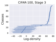
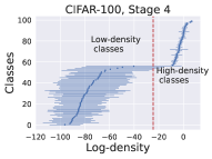
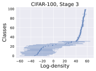
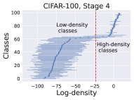
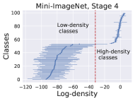
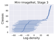
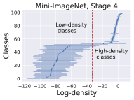
Figure 1: Mean and standard deviation of class-conditional log-densities estimated for inputs from each class. Classes on the vertical axis are sorted according to the mean class-conditional density.

We begin our analysis by characterizing representations of classes learned from the two image datasets. First, for each class $C$ and each network stage we calculate mean and standard deviation of class-conditional log-densities (Eq. 3) of examples $\mathbf{x}\in C$. Results for the third and fourth stage are reported in Fig. 1. Results for the first two stages are in the Appendix. Already, we see an unexpected structure: class representations in the last two stages display an almost phase transition-like change in class-conditional log-densities. That is, we observe two groups of classes that cluster around vastly different density values. Equally striking, classes in these groups typically differ by an order of magnitude in the standard deviation of the estimated class-conditional log-densities. Specifically, estimates for examples from the classes clustered around the higher class-conditional density typically have an order of magnitude lower variance. These observations agree between the two image datasets and the two architectures used in the experiment. Importantly, we did not found a similar structure in the representations from the first two stages, indicating that the observed phenomenon is not related to low-level features of the inputs (See Appendix). We also replicated this experiment using a plain (i.e. non-residual) convolutional network. This time we did not observe distinct modes of class fitting in any of the network layers (See Appendix). This implies that the observed structure is not simply a product of the datasets used in the experiments, but is related to the residual architecture. In summary, we observe two distinct modes of class fitting in the last two stages of ResNet models.

We now focus on the highest-level class representations, i.e. representations constructed by the last stage of the network. First, we split classes into two groups according to the estimated mean log-density values, namely low- and high-density classes (marked on Figure 1, stage 4). To this end, we sort classes according to their mean log-densities and find interval $\left(C_{i},C_{i+1}\right)$ in this sequence with the largest mean log-density difference. We use center of this interval to assign classes to the two groups. Note that we group entire classes, not individual input examples.

The most straightforward explanation for the observed differences between the uncovered groups could be that the high-density classes simply have more spatially compact distributions of neural representations. In other words, examples from these classes could have more similar high-level neural representations. Our results show that this simple explanation is incorrect. Specifically, for each class $C$ we calculated the mean distance $\|\mathrm{svd}\left(nn_{l}\left(\mathbf{x}\right)\right)-\mathrm{svd}\left(nn_{l}\left(\mathbf{y}\right)\right)\|$ between neural representations of examples $\mathbf{x},\mathbf{y}\in C$ (Eq. (1), after dimensionality reduction with SVD). We also estimated the complexity of its class representation, namely the relative entropy of its posterior predictive distribution $p\left(\bm{x^{*}}\mid\bm{x^{*}}\in C\right)$ from the reference maximum entropy distribution $q\left(\bm{x^{*}}\right)$ (Eq. (4), and the paragraph below). Results are reported in Fig. 2. Clearly, the high-density classes are not more spatially compact at the neural representation level than the low-density classes. However, their posterior predictive distributions have vastly larger complexity than the posterior predictive distributions of the low-density classes. In other words, representations of the high-density classes are vastly more non-Gaussian. Together with the high average class-conditional density of their examples, these results point to a different explanation: in representations of high-density classes, the probability mass is concentrated in a number of compact but spatially separated modes. This suggests that at the neural representation level high-density classes are formed by a collection of compact components.

ResNet18	ResNet50

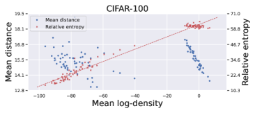
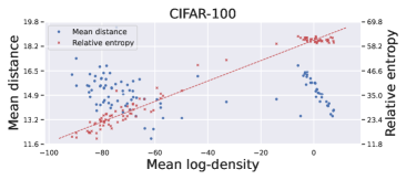
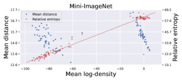
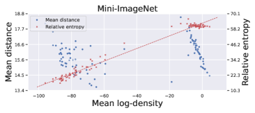
Figure 2: Relative entropies of class-conditional distributions of neural representations and mean intra-class distances between representations. Each class corresponds to one blue and one red mark. Dashed line: least-squares fit to relative entropies.

Class representations correlate with memorization and adversarial robustness

ResNet18	ResNet50

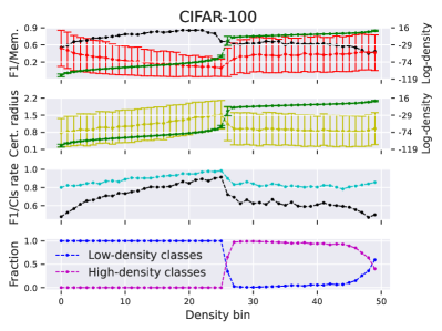
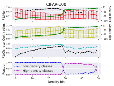
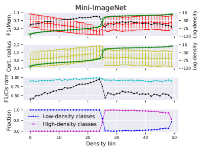
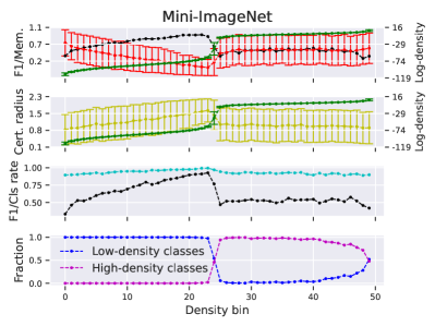
Figure 3: Relationship between class conditional log-density, input memorization and adversarial robustness. Low/high-density fraction: fraction of points in a bin from the low-/high-density classes.

Our results so far uncover an unexpected structure in the representations of learned classes. An immediate question that follows from this observation is: does this structure correlate with some phenomena observed in neural networks? We identify two such phenomena: memorization of input examples and adversarial robustness.

To demonstrate the relationship between input memorization and class representations, we sorted the training examples according to their estimated class-conditional log-density and then split this ordering into 50 equally sized bins. We then calculated for each bin the mean and the standard deviation of memorization scores and class-conditional log-densities of examples assigned to it. We also calculated the ratio of examples belonging to the low- and the high-density classes. Finally, for each bin we trained a separate ResNet model without using the training examples assigned to that bin. We then calculated the F-score of this model on the examples from the bin. Results are reported in Fig. 3.

Even though memorization scores exhibit large variance, averaging across density bins uncovers a difference in their distribution between the low- and the high-density classes. More precisely, up to the transition point between the low- and the high-density classes, the degree of memorization of an input examples decreases—on average—with increasing class-conditional log-density. This agrees with an intuition that increasing class-conditional density translates to an input example that is increasingly similar at the neural representation level to many other class members. However, the trend changes abruptly with the transition to the high-density classes. The transition is marked by an abrupt increase in average memorization of input examples, which subsequently remains largely independent of the class-conditional density. These observations are corroborated with the calculated F-scores, which are in close agreement with mean memorization scores.

At first glance, results in Fig. 3 may seem counter-intuitive. However, we argue that they corroborate the long-tail hypothesis put forward by Feldman (2020). Concretely, our results indicate that distributions of neural representations in the high-density classes have many distinct components. That is, the high-density classes are formed from smaller subpopulations of examples with distinct neural representations. The frequency of each such subpopulation in the training data will be below the class frequency. Feldman’s hypothesis suggests that in order to minimize the generalization error, the learning model may need to memorize some of the examples from these subpopulations. And indeed, we observe an increase in the degree of memorization when the distribution of input examples switches from the low- to the high-density classes.

Compact and spatially separated components in the high-density classes should—intuitively—be less robust to an adversarial attack. In particular, a relatively small input perturbation may move the representation of the attacked example outside of its component. This could be verified by comparing low- and high-density classes w.r.t the robustness against a selection of adversarial attacks. However, given the vast number of attacks proposed so far, we to opt to explore this hypothesis in an attack-agnostic way. To this end, we evaluate the performance of a provable adversarial defense in function of the class-conditional density. Concretely, we take the training examples split into density bins and for each bin train a smoothed classifier proposed by Cohen, Rosenfeld, and Kolter (2019) without using the examples from the bin. We use ResNet networks as the base (smoothed) models. We then evaluate the Certify procedure (Cohen, Rosenfeld, and Kolter 2019) for the examples from the held-out bin (See Appendix for details). The procedure either abstains from prediction or returns a certified radius $r$ and the predicted class. Importantly, Cohen, Rosenfeld, and Kolter proved that if not abstaining, Certify returns with high-probability the class that will be predicted by the smoothed classifier for inputs no further than $r$ from the certified example. Note, however, that the smoothed classifier need not agree with the base classifier. In this sense it trades classification accuracy for provable robustness.

In Fig. 3 we report per-bin certification radius (mean and standard deviation), fraction of inputs for which Certify did not abstain (classification rate) and F-score of the smoothed classifier. Results confirm that high-density classes correlate with lower adversarial robustness: transition from the low- to the high-density regime coincide with abrupt decrease in certified radii and F-scores of the smoothed classifier. Certify is also slightly more likely to abstain in high-density classes.

Where neural network fit classes

ResNet18	ResNet50

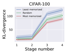
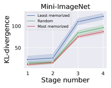
Figure 4: Kullback-Leibler divergences between class-conditional predictive densities.

We also use class-conditional distributions of neural representations to uncover where in the network architecture classes are fit and to show to what extent memorization influences this process. To this end, we selected from each dataset examples with memorization score above $0.9$. Additionally, we selected approx. equal number of examples with the lowest memorization estimates and an equal number of randomly chosen examples. We estimated the class-conditional posterior predictive distributions separately for the three chosen subsets of examples. Next, we estimated the KL divergences between predictive densities of every class pair (Eq. (4)). Note that for a pair of classes $(P,Q)$ we estimate the KL divergence from $p\left(nn_{l}\left(\mathbf{x}\right)\mid\mathbf{x}\in P\right)$ to $p\left(nn_{l}\left(\mathbf{x}\right)\mid\mathbf{x}\in Q\right)$ and the divergence from $p\left(nn_{l}\left(\mathbf{x}\right)\mid\mathbf{x}\in Q\right)$ to $p\left(nn_{l}\left(\mathbf{x}\right)\mid\mathbf{x}\in P\right)$. The asymmetry of the KL divergence therefore does not alter the conclusions of this experiment. To recover meaningful predictive densities, we restrict this analysis to classes that have at least $100$ representatives in all three subsets.

Figure 4 reports mean estimated between-class KL divergences, together with one standard deviation intervals. Additional results are reported in the Appendix. Clearly, input memorization is not fixed to some specific parts of the network: class-fitting progresses similarly for memorized and typical examples, although memorized examples induce slightly less distinct class representations. Importantly, class representations are formed mostly between the second and the third stage of the ResNet model. This agrees with the observation that distinct groups of classes are evident in the third and the fourth network stage, but not in the first two stags.

Related work

Several recent works investigate representations learned by neural networks. The first algorithm to uncover similarities between representations in these models was proposed by Raghu et al. (2017). In crux, they use SVD to remove nuisance factors from network activations, and then uncover shared representations via canonical correlation analysis. Subsequently, Morcos, Raghu, and Bengio (2018) refined this approach with a novel method for combining canonical directions, while Kornblith et al. (2019) proposed a Hilbert-Schmidt Independence Criterion-based metric for comparing neural representations. Next, Jamroż, Kurdziel, and Opala (2020) proposed probabilistic models for representations learned by kernels in convolutional networks. They showed that networks that memorize random labels learn significantly more complex representations than generalizing networks. Note that while we use a similar set of of probabilistic tools, our goal is not to characterize distributions of features learned by network units. Instead, we use class-conditional probabilistic models to capture a notion of class representations in neural networks.

A growing line of research touch on the memorization of input examples by neural networks. Zhang et al. (2017) demonstrate that neural networks can easily fit a dataset with randomly permuted labels, often despite explicit regularization during training. Arpit et al. (2017) compare networks that fit corrupted labels and networks trained on uncorrupted data with respect to the way they fit input examples. Zhang et al. (2018) proposes a new augmentation method that encourages the model to interpolate linearly between training examples. Their results suggest that such augmentation can prevent neural networks from memorizing random datasets and make them less prone to adversarial attacks. Effects of memorization were also covered by Neyshabur et al. (2017), who derived several metrics for the degree of memorization by bounding the Lipschitz constant in the model’s transformation. Finally, Feldman (2020, 2021); Feldman and Zhang (2020) propose an alternative perspective on memorization. They consider a learning task where data is assumed to follow a long-tailed distribution with many infrequent components. Feldman shows that in this scenario minimization of the generalization error requires memorizing some of the examples.

Szegedy et al. (2014) demonstrated vulnerability of neural networks to an adversarial attack. Subsequently, Goodfellow, Shlens, and Szegedy (2015) proposed a simple method for constructing adversarial examples. These results prompted significant research efforts on adversarial attacks, defence strategies and certification of models’ predictions—see Huang et al. (2020) for a recent survey.

Conclusions

In this work we used Bayesian mixture models with unknown number of components to investigate representations of classes in residual convolutional networks. Our main finding is that classes in investigated neural models are fit in two distinct ways. Namely, we uncover a group of classes in which high-level neural representations appear to form compact and spatially separated components. We showed that examples from these classes are memorized to a higher degree than examples with intermediate class-conditional log-density estimates. We also showed that these classes are less robust to an adversarial attack. Finally, we used class-conditional density models to uncover where in the network structure class representations are formed for typical and memorized examples.

Our findings gives further experimental support for the perspective on memorization proposed in (Feldman 2020; Feldman and Zhang 2020). In particular, Feldman (2020) argues that memorization of examples from infrequent components is necessary to minimize generalization error in learning tasks where data comes from a long-tailed distribution. We do observe increased memorization in classes that appear to be formed from distinct—at the neural representation level—subpopulations of examples. While we do not claim to have a theoretical explanation for why representations of these classes are so strikingly different than representations of low-density classes, we point out that current convolutional architectures evolved largely through experimental optimization of performance on several image classification benchmarks. Feldman and Zhang (2020) identify cases in these benchmarks where memorization of certain inputs improve predictions on evaluation sets. Therefore, it may simply be that convolutional networks used today were unwittingly optimized to fit classes the way we observe in this work.

Block collapsed Gibbs sampler

Standard collapsed Gibbs sampler used by Jamroż, Kurdziel, and Opala (2020), also called Plain CGS (Neal 2000; Jensen, Kjærulff, and Kong 1995), constructs a Markov chain over component assignments by sampling an assignment $c_{i}$ for one pattern $\mathbf{x}_{i}\in\mathcal{D}$ at a time:

$$c_{i}\sim p\left(c_{i}\mid\bm{c}_{t}\setminus\{i\},\bm{x}_{i},\alpha,\bm{\theta}\right),$$ (A.5)

where $\bm{c}_{t}\setminus\{i\}$ are component assignments in the current Gibbs step for all patterns except $\mathbf{x}_{i}$, and $\bm{\theta}$ is the set of parameters of the posterior distribution (over component means and covariances) induced by $\bm{c}_{t}\setminus\{i\}$. In the model given by Eq. (2) this sampling is easy, because density in Eq. (A.5) has a closed-form solution. However, since this scheme updates one assignment at a time, consecutive Gibbs steps tend to be strongly correlated. This negatively affects the rate of convergence to the posterior distribution and reduces the effective sample count in subsequent Monte Carlo estimates. In other words, plain CGS exhibits slow mixing.

To improve mixing in collapsed Gibbs sampler, one can sample blocks of component assignments. This is the idea behind block collapsed Gibbs sampler (Jensen, Kjærulff, and Kong 1995). More formally, block CGS picks in each update a group of observations $\bm{X}_{b}=\left\{\bm{x}_{i},\bm{x}_{i+1},\ldots,\bm{x}_{i+b}\right\}$, where $b$ is a fixed block size, and sample their component assignments $\bm{c}_{i\ldots i+b}=\left\{c_{i},c_{i+1},\ldots,c_{i+b}\right\}$ from the distribution:

$$\bm{c}_{i\ldots i+b}\sim p\left(\bm{c}_{i\ldots i+b}\mid\bm{c}_{t}\setminus\left\{i,i+1,\ldots,i+b\right\},\bm{X}_{b},\alpha,\bm{\theta}\right).$$ (A.6)

Assignments $c_{i},c_{i+1},\ldots,c_{i+b}$ are sampled independently. For the model given by Eq. (2), the density in (A.6) again has a closed-form solution.

In this work we use block CGS in all experiments involving estimation of posterior predictive distributions and related quantities. There are many strategies to form the blocks of observations for sampling. For example, Wilkinson and Yeung (2002) discuss several strategies designed to improve mixing rate in highly structured conditional models. Our strategy for splitting observations into blocks is simple: before every pass over the dataset, we randomly permute observations $\bm{x}_{1},\bm{x}_{2},\ldots,\bm{x}_{n}$ and then form blocks $\bm{X}_{b}$ by iterating over this permutation and taking consecutive $b$-sized batches of observations.

ResNet representations

ResNet architecture reduces spatial dimensions in four stages. We calculate neural representations from the output of the summation operation at the end of each stage (Fig. A.5). Main results in this work focus on the representations calculated from the last stage, namely input to the classification head.

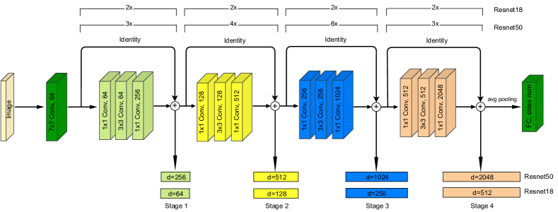
Figure A.5: Activation vectors used in this work. ResNet architecture has four stages that correspond to progressively smaller spatial dimensions. We extract activations at the end of each of these stages.

To reduce the computational cost of estimating full-covariance Gaussian mixture models, we reduce the dimensionality of the collected neural representations via Singular Value Decomposition (SVD). That is, we use SVD to decompose the $n\times d$ matrix that contains neural representations arranged in rows, and then project the data onto a subset of right-singular vectors corresponding to the largest singular values. We retain $d^{\prime}=16$ right-singular vectors for the first two ResNet stages and $d^{\prime}=64$ for the third and fourth stage. This allows us to capture most of the variance in the collected sets of neural representations (Fig. A.6) and is sufficient to uncover differences between representations of classes.

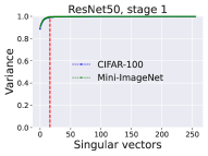
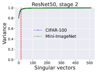
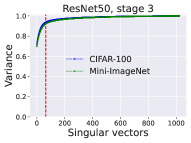
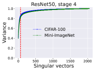
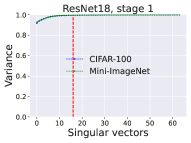
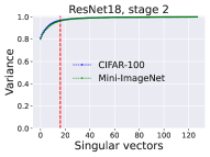
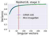
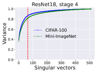
Figure A.6: Variance in network activations captured by SVD in function of the number of singular vectors. Red dashed line marks the number of singular vectors retained in each network stage.

Evaluation of adversarial robustness

For each density bin we train a smoothed classifier proposed by Cohen, Rosenfeld, and Kolter (2019) using examples from the bin as held-out data. We use ResNet18 and ResNet50 networks as baseline models for smoothing. We use the same training setup as in main experiments, i.e. we follow training hyper-parameters reported by (Feldman and Zhang 2020). However, as suggested by Cohen, Rosenfeld, and Kolter (2019) we add Gaussian noise to the input augmentation pipeline. We use a noise strength $\sigma=0.5$.

We evaluate Certify (Cohen, Rosenfeld, and Kolter 2019) with $n_{0}=100$ and $n=10^{5}$ samples. We certify with the Gaussian noise $\sigma=0.5$ and the probability of incorrect answer $\alpha=10^{-3}$.

Distinct modes of class fitting in residual convolutional networks

ResNet18

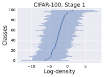
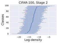
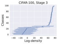
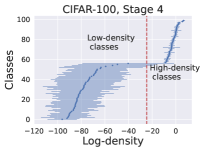
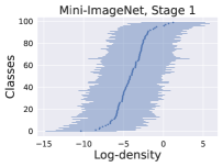
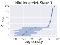
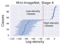
ResNet50

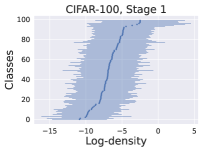
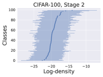
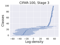
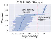
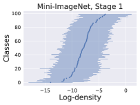
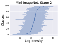
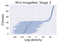
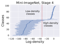
Figure A.7: Mean and standard deviation of class-conditional log-densities estimated for inputs from each class. Classes on the vertical axis are sorted according to the mean class-conditional density.

Plain ConvNet, CIFAR100


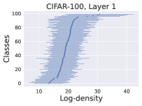
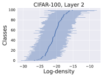
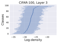
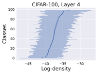
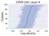
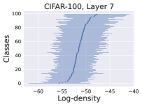
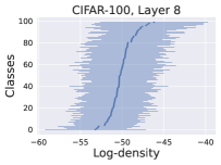
Plain ConvNet, Mini-ImageNet

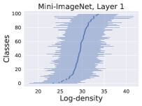
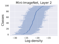
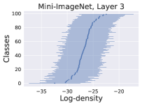
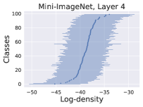
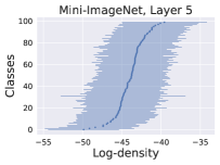
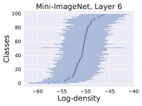
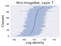
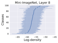
Figure A.8: Mean and standard deviation of class-conditional log-densities estimated for representations from a plan 8-layer convolutional network.

In the initial two stages of a ResNet model classes are mostly indistinguishable with respect to the class-conditional log-densities of neural representations (Fig. A.7). However, in the third and fourth stage we observe two distinct groups of classes that cluster around different mean log-density values. The two groups also differ in variance of the estimated log-densities. In principle, this structure could be simply a product of the datasets used in experiments. However, our results show that this is not the case. Specifically, we replicated our experiments using a plain (i.e. non-residual) 8-layer convolutional network. This model fits classes in an uniform way across all hidden layers (Fig. A.8).

Our results suggests that classes with high mean log-density values are formed by collections of compact but spatially separated components. This raises a following question: is this component structure observed in the posterior over parameters of the model in Eq. (2)? We do observe that posterior samples in the CGS chains for the high-density classes involve many more components than samples for the low-density classes. However, we do not report these numbers, as estimation of component counts is fragile. Concretely, the model in Eq. (2) is an infinite mixture. As such, it is consistent for the density, but is not consistent for the number of components (Miller and Harrison 2014). While there are mixture models consistent for the number of components (Miller and Harrison 2018), they require knowledge of the components’ distribution. Any misspecification of this base distribution would lead to incorrect estimates for component counts.

Class representations in Vision Transformers and MLP-Mixers

The striking difference between class representations in ResNets and plain convolutional networks suggests that other architectures with residual connections may also display non-trivial structure in neural representations. Here we report our initial findings for two such architectures, namely Vision Transformer (ViT) (Dosovitskiy et al. 2021) and MLP-Mixer (Tolstikhin et al. 2021). Specifically, we took the ViT-B/16 and Mixer-B/16 models pre-trained on the ImageNet dataset with Sharpness-aware Minimization (Foret et al. 2021) and fine-tuned them to CIFAR100 and Mini-ImageNet classes. Vision Transformer models typically contain a separate class token. To form class representations for the ViT-B/16 network we therefore fitted density models to class token activations extracted at the end of each encoder block. MLP-Mixer models construct input to the classification head by global average pooling of activation maps. Consequently, in this case we fitted density models to activations formed by global average pooling of each mixer block output. When fitting density models we followed the procedure used for ResNets, including dimensionality reduction and a weakly-informative prior distribution.

Similarly to ResNets, initial layers in ViT and Mixer-MLP models do not display any unexpected structure in class conditional distributions of neural representations (Fig. A.9 and Fig. A.10). The picture changes in deeper layers. First, we observe layers where class representations display structure similar to the one observed in ResNets, namely low- and high-density modes. However, we also observe layers where all classes exhibit a relatively low (compared to initial layers) variance in class conditional densities of neural representations. How this structure influences memorization and adversarial robustness in these models remains an open question. Specifically, while replication the complete set of our experiments is conceptually simple, the computational cost of training ViT and Mixer-MLP models makes calculation of required memorization and adversarial robustness scores challenging.

Vision Transformer, CIFAR100



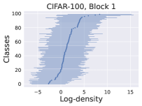
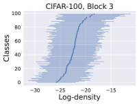
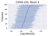
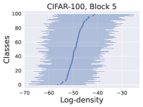
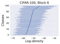
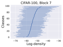
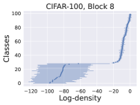
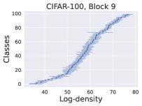
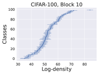
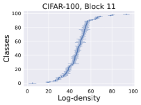
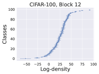
Vision Transformer, Mini-ImageNet

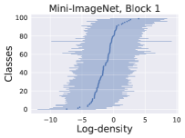
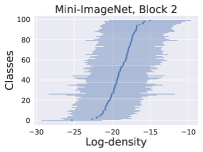
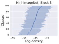
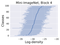
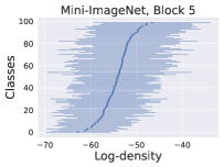
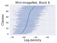
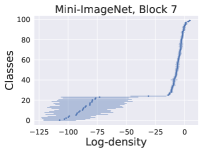
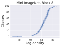
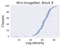
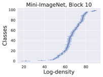
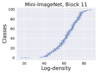
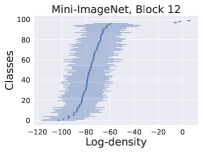
Figure A.9: Mean and standard deviation of class-conditional log-densities estimated for representations from a 12-block Vision Transformer model.

MLP-Mixer, CIFAR100



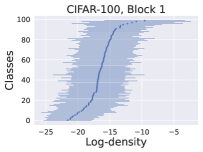
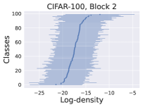
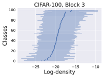
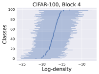
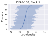
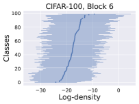
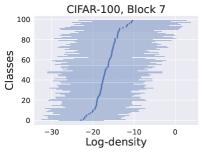
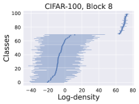
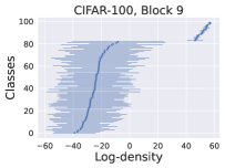
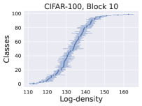
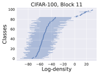
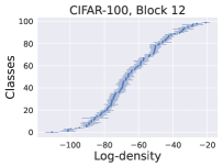
MLP-Mixer, Mini-ImageNet

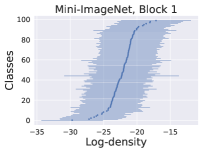
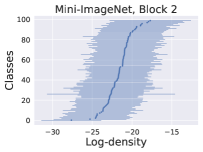
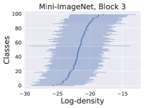
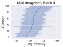
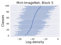
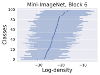
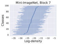
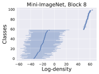
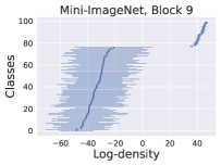
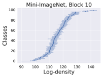
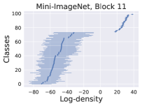
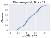
Figure A.10: Mean and standard deviation of class-conditional log-densities estimated for representations from a 12-block MLP-Mixer model.

Where neural network fit classes

Results reported in Fig. 4 can be replicated with a generative classifier derived from the class-conditional densities:

$$C=\operatorname*{arg\,max}_{C}p\left(nn_{l}\left(\mathbf{x}\right)\mid\mathbf{x}\in C\right)p(C),$$ (A.7)

where the prior $p(C)$ comes from empirical class frequencies. More precisely, one can select a set of held-out examples, fit class-conditional predictive densities to the remaining data points and predict classes for the held-out examples. Figure A.11 reports F-scores for generative classification of $1,000$ most memorized examples, an equal number of randomly selected examples, and an equal number of randomly selected examples with no memorization (i.e. memorization estimate equal to $0.0$). Generative classification recover classes of held-out inputs and its performance is compatible with the between-class divergences reported in Fig. 4.

ResNet18	ResNet50

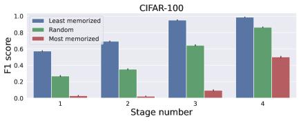
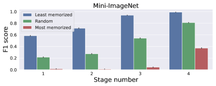
Figure A.11: F-scores for generative classification (Eq. (A.7)) of memorized examples, examples with no memorization, and randomly selected examples.

Feldman and Zhang (2020) reported negative result in an experiment designed to test whether estimation of memorization scores can be speed-up by sharing a common convolutional backbone across all trained models, and only fitting the ultimate fully-connected layer. Our results concerning fitting of memorized examples suggest that other strategies of this kind are also likely to fail.

Computational cost of experiments

All neural networks used in this work were trained on NVIDIA Tesla V100 GPUs, with one training run taking under 2 hour on a single GPU. Density models were estimated on 24-core Intel Haswell nodes equipped with 128 GB of RAM. A typical collapsed Gibbs sampler run in these settings takes between 1 and 3 days, depending on the input dimensionality. Computing infrastructure used in this work runs under CentOS Linux release 7.9. Versions of all required libraries and software packages are provided as an environment definition alongside the source code for replicating the experiments.

References

- Arpit et al. (2017) Arpit, D.; Jastrzebski, S.; Ballas, N.; Krueger, D.; Bengio, E.; Kanwal, M. S.; Maharaj, T.; Fischer, A.; Courville, A. C.; Bengio, Y.; and Lacoste-Julien, S. 2017. A Closer Look at Memorization in Deep Networks. In Proceedings of the 34th International Conference on Machine Learning, ICML 2017, Sydney, NSW, Australia, 6-11 August 2017, 233–242.
- Cohen, Rosenfeld, and Kolter (2019) Cohen, J. M.; Rosenfeld, E.; and Kolter, J. Z. 2019. Certified Adversarial Robustness via Randomized Smoothing. In Chaudhuri, K.; and Salakhutdinov, R., eds., Proceedings of the 36th International Conference on Machine Learning, ICML 2019, 9-15 June 2019, Long Beach, California, USA, volume 97 of Proceedings of Machine Learning Research, 1310–1320. PMLR.
- Dosovitskiy et al. (2021) Dosovitskiy, A.; Beyer, L.; Kolesnikov, A.; Weissenborn, D.; Zhai, X.; Unterthiner, T.; Dehghani, M.; Minderer, M.; Heigold, G.; Gelly, S.; Uszkoreit, J.; and Houlsby, N. 2021. An Image is Worth 16x16 Words: Transformers for Image Recognition at Scale. In 9th International Conference on Learning Representations, ICLR 2021, Virtual Event, Austria, May 3-7, 2021.
- Feldman (2020) Feldman, V. 2020. Does Learning Require Memorization? A Short Tale about a Long Tail. In Proceedings of the 52nd Annual ACM SIGACT Symposium on Theory of Computing, STOC 2020, 954–959. Association for Computing Machinery.
- Feldman (2021) Feldman, V. 2021. Does Learning Require Memorization? A Short Tale about a Long Tail. arXiv preprint arXiv:1906.05271.
- Feldman and Zhang (2020) Feldman, V.; and Zhang, C. 2020. What Neural Networks Memorize and Why: Discovering the Long Tail via Influence Estimation. In Advances in Neural Information Processing Systems 33: Annual Conference on Neural Information Processing Systems 2020, NeurIPS 2020, December 6-12, 2020, virtual.
- Foret et al. (2021) Foret, P.; Kleiner, A.; Mobahi, H.; and Neyshabur, B. 2021. Sharpness-aware Minimization for Efficiently Improving Generalization. In 9th International Conference on Learning Representations, ICLR 2021, Virtual Event, Austria, May 3-7, 2021.
- Ghosal and Van der Vaart (2017) Ghosal, S.; and Van der Vaart, A. 2017. Fundamentals of nonparametric Bayesian inference. Cambridge Series in Statistical and Probabilistic Mathematics. Cambridge University Press.
- Goodfellow, Shlens, and Szegedy (2015) Goodfellow, I. J.; Shlens, J.; and Szegedy, C. 2015. Explaining and Harnessing Adversarial Examples. In 3rd International Conference on Learning Representations, ICLR 2015, San Diego, CA, USA, May 7-9, 2015.
- Huang et al. (2020) Huang, X.; Kroening, D.; Ruan, W.; Sharp, J.; Sun, Y.; Thamo, E.; Wu, M.; and Yi, X. 2020. A survey of safety and trustworthiness of deep neural networks: Verification, testing, adversarial attack and defence, and interpretability. Computer Science Review, 37(100270).
- Jamroż, Kurdziel, and Opala (2020) Jamroż, M.; Kurdziel, M.; and Opala, M. 2020. A Bayesian Nonparametrics View into Deep Representations. In Advances in Neural Information Processing Systems 33: Annual Conference on Neural Information Processing Systems 2020, NeurIPS 2020, December 6-12, 2020, virtual.
- Jensen, Kjærulff, and Kong (1995) Jensen, C. S.; Kjærulff, U.; and Kong, A. 1995. Blocking Gibbs sampling in very large probabilistic expert systems. Int. J. Hum. Comput. Stud., 42(6): 647–666.
- Kornblith et al. (2019) Kornblith, S.; Norouzi, M.; Lee, H.; and Hinton, G. E. 2019. Similarity of Neural Network Representations Revisited. In Proceedings of the 36th International Conference on Machine Learning, ICML 2019, 9-15 June 2019, Long Beach, California, USA, 3519–3529.
- Krizhevsky (2009) Krizhevsky, A. 2009. Learning multiple layers of features from tiny images. Technical report.
- Miller and Harrison (2014) Miller, J. W.; and Harrison, M. T. 2014. Inconsistency of Pitman-Yor Process Mixtures for the Number of Components. J. Mach. Learn. Res., 15(96): 3333–3370.
- Miller and Harrison (2018) Miller, J. W.; and Harrison, M. T. 2018. Mixture Models With a Prior on the Number of Components. J. Am. Stat. Assoc., 113(521): 340–356.
- Morcos, Raghu, and Bengio (2018) Morcos, A. S.; Raghu, M.; and Bengio, S. 2018. Insights on representational similarity in neural networks with canonical correlation. In Advances in Neural Information Processing Systems 31: Annual Conference on Neural Information Processing Systems 2018, 3-8 December 2018, Montréal, Canada, 5732–5741.
- Neal (2000) Neal, R. M. 2000. Markov chain sampling methods for Dirichlet process mixture models. J. Comput. Graph. Stat., 9(2): 249–265.
- Neyshabur et al. (2017) Neyshabur, B.; Bhojanapalli, S.; McAllester, D.; and Srebro, N. 2017. Exploring Generalization in Deep Learning. In Advances in Neural Information Processing Systems 30: Annual Conference on Neural Information Processing Systems 2017, December 4-9, 2017, Long Beach, CA, USA, 5947–5956.
- Raghu et al. (2017) Raghu, M.; Gilmer, J.; Yosinski, J.; and Sohl-Dickstein, J. 2017. SVCCA: Singular Vector Canonical Correlation Analysis for Deep Learning Dynamics and Interpretability. In Advances in Neural Information Processing Systems 30: Annual Conference on Neural Information Processing Systems 2017, 4-9 December 2017, Long Beach, CA, USA, 6076–6085.
- Szegedy et al. (2014) Szegedy, C.; Zaremba, W.; Sutskever, I.; Bruna, J.; Erhan, D.; Goodfellow, I. J.; and Fergus, R. 2014. Intriguing properties of neural networks. In 2nd International Conference on Learning Representations, ICLR 2014, Banff, AB, Canada, April 14-16, 2014.
- Tolstikhin et al. (2021) Tolstikhin, I. O.; Houlsby, N.; Kolesnikov, A.; Beyer, L.; Zhai, X.; Unterthiner, T.; Yung, J.; Steiner, A.; Keysers, D.; Uszkoreit, J.; Lucic, M.; and Dosovitskiy, A. 2021. MLP-Mixer: An all-MLP Architecture for Vision. In Advances in Neural Information Processing Systems 34: Annual Conference on Neural Information Processing Systems 2021, NeurIPS 2021, December 6-14, 2021, virtual, 24261–24272.
- Vinyals et al. (2016) Vinyals, O.; Blundell, C.; Lillicrap, T.; Kavukcuoglu, K.; and Wierstra, D. 2016. Matching Networks for One Shot Learning. In Advances in Neural Information Processing Systems 29: Annual Conference on Neural Information Processing Systems 2016, December 5-10 2016, Barcelona, Spain, 3630–3638.
- Wilkinson and Yeung (2002) Wilkinson, D. J.; and Yeung, S. K. H. 2002. Conditional simulation from highly structured Gaussian systems, with application to blocking-MCMC for the Bayesian analysis of very large linear models. Statistics and Computing, 12(3): 287–300.
- Zhang et al. (2017) Zhang, C.; Bengio, S.; Hardt, M.; Recht, B.; and Vinyals, O. 2017. Understanding deep learning requires rethinking generalization. In 5th International Conference on Learning Representations, ICLR 2017, Toulon, France, April 24-26, 2017.
- Zhang et al. (2018) Zhang, H.; Cissé, M.; Dauphin, Y. N.; and Lopez-Paz, D. 2018. mixup: Beyond Empirical Risk Minimization. In 6th International Conference on Learning Representations, ICLR 2018, Vancouver, BC, Canada, April 30 - May 3, 2018.