Shamel Fahmi

On Terrain-Aware Locomotion for Legged Robots

Doctor of Philosophy (PhD) in Bioengineering and Robotics

Curriculum: Advanced and Humanoid Robotics

Dynamic Legged Systems (DLS) lab, Italian Institute of Technology (IIT), Italy

 

Tutors:

Dr. Victor Barasuol, Dr. Michele Focchi, and Dr. Andreea Radulescu

Dynamic Legged Systems (DLS) lab, Italian Institute of Technology (IIT), Italy

Principle Advisor:

Dr. Claudio Semini

Dynamic Legged Systems (DLS) lab, Italian Institute of Technology (IIT), Italy

 

Annual Evaluation Committee:

Prof. Roy Featherstone

Advanced Robotics (ADVR) department, Italian Institute of Technology (IIT), Italy

Dr. Enrico Mingo

Humanoids & Human Centered Mechatronics (HHCM) lab, Italian Institute of Technology (IIT), Italy

Dr. Geoff Fink

Dynamic Legged Systems (DLS) lab, Italian Institute of Technology (IIT), Italy

 

External Examination Committee:

Prof. Auke Ijspeert

Institute of Bioengineering, the Swiss Federal Institute of Technology at Lausanne (EPFL), Switzerland

Prof. Luis Sentis

Department of Aerospace Engineering and Engineering Mechanics, University of Texas, USA

Prof. Fabio Ruggiero

Department of Electrical Engineering and Information Technology, University of Naples Federico II, Italy

 

© 2021 Shamel Fahmi. All rights reserved.

To my parents Amal and Prof. Shamel,
to my grandmother Hagougi,
to my siblings Menna and Mohamed,
to our family’s latest member Selim,
and to my partner Ilef.

Abstract

Legged robots are advancing towards being fully autonomous as can be seen by the recent developments in academia and industry. To accomplish breakthroughs in dynamic whole-body locomotion, and to be robust while traversing unexplored complex environments, legged robots have to be terrain aware.

Terrain-Aware Locomotion (TAL) implies that the robot can perceive the terrain with its sensors, and can take decisions based on this information. The decisions can either be in planning, control, or in state estimation, and the terrain may vary in geometry or in its physical properties. TAL can be categorized into Proprioceptive Terrain-Aware Locomotion (PTAL), which relies on the internal robot measurements to negotiate the terrain, and Exteroceptive Terrain-Aware Locomotion (ETAL) that relies on the robot’s vision to perceive the terrain. This thesis presents TAL strategies both from a proprioceptive and an exteroceptive perspective. The strategies are implemented at the level of locomotion planning, control, and state estimation, and are using optimization and learning techniques.

The first part of this thesis focuses on PTAL strategies that help the robot adapt to the terrain geometry and properties. At the Whole-Body Control (WBC) level, achieving dynamic TAL requires reasoning about the robot dynamics, actuation and kinematic limits as well as the terrain interaction. For that, we introduce a Passive Whole-Body Control (pWBC) framework that allows the robot to stabilize and walk over challenging terrain while taking into account the terrain geometry (inclination) and friction properties. The pWBC relies on rigid contact assumptions which makes it suitable only for stiff terrain. As a consequence, we introduce Soft Terrain Adaptation aNd Compliance Estimation (STANCE) which is a soft terrain adaptation algorithm that generalizes beyond rigid terrain. STANCE consists of a Compliant Contact Consistent Whole-Body Control (c³WBC) that adapts the locomotion strategies based on the terrain impedance, and an online Terrain Compliance Estimator (TCE) that senses and learns the terrain impedance properties to provide it to the c³WBC. Additionally, we demonstrate the effects of terrains with different impedances on state estimation for legged robots.

The second part of the thesis focuses on ETAL strategies that makes the robot aware of the terrain geometry using visual (exteroceptive) information. To do so, we present Vision-Based Terrain-Aware Locomotion (ViTAL) which is a locomotion planning strategy. ViTAL consists of a Vision-Based Pose Adaptation (VPA) algorithm to plan the robot’s body pose, and a Vision-Based Foothold Adaptation (VFA) algorithm to select the robot’s footholds. The VFA is an extension to the state of the art in foothold selection planning strategies. Most importantly, the VPA algorithm introduces a different paradigm for vision-based pose adaptation. ViTAL relies on a set of robot skills that characterizes the capabilities of the robot and its legs. These skills are then learned via self-supervised learning using Convolutional Neural Networks (CNNs). The skills include (but are not limited to) the robot’s ability to assess the terrain’s geometry, avoid leg collisions, and to avoid reaching kinematic limits. As a result, we contribute with an online vision-based locomotion planning strategy that selects the footholds based on the robot capabilities, and the robot pose that maximizes the chances of the robot succeeding in reaching these footholds.

Our strategies are based on optimization and learning methods, and are extensively validated on the quadruped robots HyQ and HyQReal in simulation and experiment. We show that with the help of these strategies, we can push dynamic legged robots one step closer towards being fully autonomous and terrain aware.

Preface

• This doctoral thesis is building upon decades of research and development in robotics, dynamics, controls, and machine learning. We expect that the reader has a basic knowledge about legged robotics before reading this thesis.

• This doctoral thesis is styled as a cumulative thesis. The main contents are based on publications from peer-reviewed journals, with an exception of one chapter that contains yet unpublished material. Chapter 1 gives a brief introduction to the problem and the state of the art, and it lists the contributions and the outline of the thesis. Chapters 2, 3, and 4 include the peer-reviewed publications while Chapter 5 includes the yet to be published one. Finally, Chapter 7 concludes this thesis with a discussion and a summary of this work and its future directions.

• The articles that Chapters 2-5 are based on are my original work as a first author. However, these articles are also the fruit of the effort of the supervisors and co-authors that assisted me during the period of my PhD. For this reason, I decided to use the active plural voice (we and our) instead of the singular voice (I and my) throughout the text.

• Chapter 2 has been published in [1]. The concept and theory of this work has been developed by myself and M. Focchi. The formulation and implementation has been developed by myself with the support of M. Focchi. The experiments were conducted and analyzed by M. Focchi with the support of C. Mastalli and myself. The manuscript was written by myself with the support of M. Focchi and C. Mastalli, and was reviewed by C. Semini.

• Chapter 3 has been published in [2]. The concept and theory of this work has been developed by myself and M. Focchi. The formulation and implementation has been developed by myself with the support of M. Focchi and A. Radulescu. The experiments were conducted and analyzed by myself with the support of M. Focchi and G. Fink. The manuscript was written by myself with the support of M. Focchi and G. Fink, and it was reviewed by A. Radulescu, V. Barasuol, and C. Semini.

• Chapter 4 has been published in [3]. The concept and theory of this work has been developed by myself with the support of G. Fink. The formulation and implementation has been developed by myself with the support of G. Fink. The experiments were conducted and analyzed by myself and G. Fink. The manuscript was written by myself and G. Fink and was reviewed by C. Semini.

• Chapters 5 and 6 have been published in [4]. The concept and theory of this work has been developed by myself and V. Barasuol. The formulation and implementation has been developed by myself with the support of D. Esteban, O. Villarreal, and V. Barasuol. The experiments were conducted and analyzed by myself with the support of V. Barasuol. The manuscript was written by myself with the support of V. Barasuol, and it was reviewed by D. Esteban, O. Villarreal, and C. Semini. Note that, part of this chapter has been revised after the defense date.

• The style of this dissertation has been adopted from A. Winkler’s dissertation [5].

Contents

toc

List of Figures

lof

List of Tables

lot

Acronyms

AtI

Athletic Intelligence

c³WBC

Compliant Contact Consistent Whole-Body Control

c³

compliant contact consistent

CI

Cognitive Intelligence

CNN

Convolutional Neural Network

CoM

Center of Mass

DoFs

Degrees of Freedom

RL

Reinforcement Learning

EKF

Extended Kalman Filter

ETAL

Exteroceptive Terrain-Aware Locomotion

FC

Foot Trajectory Collision

$\mathcal{F}$

Set of Safe Footholds

FEC

Foothold Evaluation Criteria

GES

Globally Exponentially Stable

GRFs

Ground Reaction Forces

HAA

Hip Adduction-Abduction

HC

Hunt and Crossley’s

HFE

Hip Flexion-Extension

HyQ

Hydraulically actuated Quadruped

HyQReal

IMU

Inertial Measurement Unit

KFE

Knee Flexion-Extension

KF

Kinematic Feasibility

KV

Kelvin-Voigt’s

LC

Leg Collision

LF

Left-Front

LH

Left-Hind

LTV

Linear Time-Varying

MAE

Mean Absolute Tracking Error

MCS

Motion Capture System

MPC

Model Predictive Control

NLO

Non-Linear Observer

$\mathrm{n_{sf}}$

Number of Safe Footholds

ODE

Open Dynamics Engine

PE

Persistency of Excitation

PTAL

Proprioceptive Terrain-Aware Locomotion

pWBC

Passive Whole-Body Control

QP

Quadratic Program

RCF

Reactive Controller Framework

RF

Right-Front

RH

Right-Hind

STANCE

Soft Terrain Adaptation aNd Compliance Estimation

TCE

Terrain Compliance Estimator

sWBC

Standard Whole-Body Control

TAL

Terrain-Aware Locomotion

TBR

Terrain-Based Body Reference

TO

Trajectory Optimization

TR

Terrain Roughness

VFA

Vision-Based Foothold Adaptation

ViTAL

Vision-Based Terrain-Aware Locomotion

VPA

Vision-Based Pose Adaptation

WBC

Whole-Body Control

WBOpt

Whole-Body Optimization

XKF

eXogeneous Kalman Filter

ZMP

Zero Moment Point

Chapter 1  Introduction

Marc Raibert gave a broad definition of intelligence in a recent talk, and divided it into: Cognitive Intelligence (CI) and Athletic Intelligence (AtI) [6]. CI allows us to make abstract plans, and to understand and solve broader problems. AtI on the other hand, allows us to operate our bodies in such a way that we can balance, stand, walk, climb, etc. AtI also lets us do real-time perception so that we can interact with the world around us. Marc also noted that although not all of us are athletes, we still have a great amount of AtI in us. This thesis is about AtI for legged robots; it can perhaps be one step towards reaching animal-level AtI.

1.1  Motivation

Legged robots have been around for decades. Recently however, they have shown remarkable agile capabilities thanks to the research efforts of academia and industry. For this reason, legged robots are moving out of research labs into the real world with the promise of being athletically intelligent. The promise is that legged robots are to aid humans in various applications. The applications include (but are not limited to) warehouse logistics, inspection at industrial plants and construction sites, search and rescue, agriculture, package delivery, space exploration, etc. In all of these applications, there is perhaps one thing in common: none of the terrains that the robots traverse are the same. In fact, these terrains are usually dynamic, unexplored, and uncertain. As a result, the core problem is that the terrain that robots traverse introduces a large amount of uncertainty. Therefore, for legged robots to achieve AtI and accomplish breakthroughs in dynamic whole-body locomotion, they have to be terrain aware.

Terrain-Aware Locomotion (TAL) means that the robot is able to perceive and understand the surrounding terrain, and is able to take decisions based on that. In other words, the robot has to have a good knowledge of its surroundings and use whatever sensors it has to perceive these surroundings and act upon them. The terrain itself may vary in its geometry or in its physical properties, and the decisions can either be in planning, control, or in state estimation. To clarify, let us raise the following questions:

• Can the robot sense (see and feel) the world around it, and the terrain it is traversing?

• Can the robot understand the differences between the geometrical and physical properties of the terrain it is traversing?

• Can the robot plan its motion based on its understanding of the terrain and its own limitations?

• Can the robot quickly adapt this planned motion in case something goes wrong with it (such as falling, slipping, external pushes, etc.)?

If the answer is yes, then the robot is terrain aware.

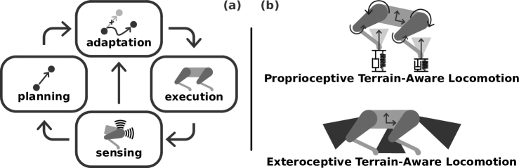
Figure 1.1: The Bigger Picture of Locomotion for Legged Robots. (a) an overview of the pipeline used in locomotion strategies for legged robots. (b) an illustration of the two categories of Terrain-Aware Locomotion (TAL).

1.2  The Bigger Picture

This section provides a broad overview of the pipeline used in locomotion strategies for legged robots, and details on each block. As shown in Fig. 1.1(a), the pipeline has four main modules: sensing, planning, adaptation and execution.

Sensing:  This is the perception module that encapsulates all of the robot’s ability to perceive itself and its surroundings. For that, the robot relies on its onboard sensors to measure its base and joint states, and build a map of its surroundings. These onboard sensors include IMUs, joint encoders, torque sensors, as well as its onboard LIDARs and cameras.

Planning:  This is the trajectory generation module that plans the motion of the robot. The goal of the planning module is to understand the perceived information from the sensing module, and plan a motion for the robot to take accordingly. This motion tends to be a long term horizon motion.

Adaptation:  The adaption module acts as an intermediate module between the planning and execution modules. This module tends to be usually merged with the planning module. However, it is important to understand the core differences between both. The adaptation module has a re-planning nature. This means that if the planned motion is not executed as programmed, or if something goes wrong during execution (such as if the robots falls, slips or gets disturbed or pushed), the adaptation module can be able to sense this right away, and adapt the robot’s motion accordingly.

Execution:  After perceiving the sensed information, and after planning and adapting the robot’s motion, the robot finally gets to execute this motion at the joint level. Hence, the robot has to track its desired whole-body states while reasoning about its own dynamics and limits, and about the surrounding terrain.

1.3  Terrain-Aware Locomotion (TAL)

TAL can be categorize into Proprioceptive Terrain-Aware Locomotion (PTAL) and Exteroceptive Terrain-Aware Locomotion (ETAL) as shown in Fig. 1.1(b). PTAL relies on the internal robot measurements (mainly its whole body states) to acquire the terrain information that is surrounding the robot. ETAL relies on directly acquiring this information using the robot’s visual sensing.

An early work on PTAL was on reflex actions that reactively adapt the swinging legs trajectory to overcome obstacles if a collision is detected [7]. Since proprioceptive sensors measures the internal robot states, detecting and localizing contacts on the robot is possible. For instance, some PTAL strategies rely on the joint position, velocity and/or torque measurements to detect and localize contacts [8, 9, 10], and to detect slippage [11, 12]. In addition to the terrain’s geometry, PTAL strategies are also used to infer and adapt to the physical properties of the terrain. For instance, several works have adopted PTAL strategies in locomotion planning and control over different terrain impedance parameters [13, 2, 14]. In these works, the robot was able to detect changes in the terrain impedance, and act upon it online.

PTAL strategies are useful in many scenarios when visual feedback is denied (such as smoky areas, or areas with thick vegetation) or when the terrain map is unreliable. However, based on their proprioceptive nature, the actions from PTAL strategies are limited to corrective actions because predicting future robot-terrain interactions using only the robot’s internal states is insufficient. This means that PTAL strategies do not act on what is ahead of the robot. Hence, an action has to happen first before triggering a reactive strategy; the foot has to collide before triggering a step reflex, or touch the terrain before inferring its physical properties.

Unlike PTAL, ETAL relies mainly on visual information. This gives ETAL strategies the advantage of looking ahead of the robot. One famous ETAL strategy is in selecting the best footholds based on the terrain information and the capabilities of the legs. This is often referred to as foothold selection [15, 16, 17, 18]. Apart from foothold selection and similar to PTAL, ETAL strategies have also been used to infer the terrain properties from images using deep learning [19, 20, 21].

1.4  Contributions

This thesis summaries our work done on TAL for legged robots. Our work includes strategies implemented for both PTAL and ETAL, and is applied at the levels of planning, control, and state estimation. This thesis is divided into two parts. The first part focuses on PTAL and the second part focuses on ETAL. This thesis is based on four main articles papers [1, 2, 3, 4]. Each article is self-contained and is included in a stand-alone chapter. The remainder of this section summarizes the motivation and contributions of each of these articles.

C1: Passive Whole-Body Control for Quadruped Robots

To achieve AtI as explained earlier in this chapter, the locomotion strategy should be able to reason about the robot’s capabilities, and to be terrain aware. Thus, as a first step, the first paper contributes to PTAL strategies by presenting a Whole-Body Control (WBC) framework.

This paper presents a Passive Whole-Body Control (pWBC) framework for quadruped robots, and focuses on the experimental validation. The pWBC is aware of the terrain geometry and friction properties. Additionally, the pWBC achieves dynamic locomotion while compliantly balancing the robot’s trunk. To do so, we formulate the motion tracking as a Quadratic Program (QP) that takes into account the full robot rigid body dynamics, the actuation limits, the joint limits and the contact interaction. To be terrain aware, we encode the terrain geometry (inclination), and frictional properties in the QP formulation. To maintain contact consistency with the rigid terrain, we also encode the rigid contact interaction in the QP formulation.

To validate the approach used in this paper, we analyze the pWBC’s robustness against inaccurate terrain friction properties, and the robot’s ability to adapt to any sudden change in the actuation limits. We also present extensive experimental trials on the HyQ robot, and validate the PTAL capabilities of the pWBC under various terrain conditions and gaits. The paper also includes extensive implementation details gained from the experience with the real platform.

C2: STANCE: Locomotion Adaptation over Soft Terrain

Remark 1.1

This work has been selected as a finalist for the IEEE RAS Italian Chapter Young Author Best Paper Award 2020, and for the IEEE RAS Technical Committee on Model-Based Optimization for Robotics Best Paper Award 2020.

The previous paper presented a pWBC framework that was rigid contact consistent. In other words, the pWBC was terrain aware with respect to rigid terrain. In fact, most of WBC frameworks fail to generalize beyond rigid terrains. To be terrain aware, the robot should be able to adapt to terrains with different impedances. For that, we focused on extending the PTAL capabilities of the previously presented pWBC, and adapting it to multiple terrains with different impedances (such as soft terrain). We study compliant terrain since it is an unsolved issue for legged locomotion. Legged locomotion over soft terrain is difficult because of the presence of unmodeled contact dynamics that standard WBCs do not account for. This introduces uncertainty in locomotion and affects the stability and performance of the system.

Therefore, this paper proposes a novel soft terrain adaptation algorithm called Soft Terrain Adaptation aNd Compliance Estimation (STANCE). From its name, STANCE consists of a Compliant Contact Consistent Whole-Body Control (c³WBC) that is aware of the terrain impedance, and an online Terrain Compliance Estimator (TCE) that senses and estimates the terrain impedance. The c³WBC exploits the knowledge of the terrain to generate an optimal solution that is contact consistent. This terrain knowledge is provided to the c³WBC by the TCE.

In this paper, we show that STANCE can adapt online to any type of terrain compliance (stiff or soft). To do so, we evaluated STANCE both in simulation and experiment on HyQ, and we compared it with the state of the art pWBC from the previous paper. We demonstrated the capabilities of STANCE with multiple terrains of different compliances, with aggressive maneuvers, different forward velocities, and external disturbances. STANCE allowed HyQ to adapt online to terrains with different compliances (rigid and soft) without pre-tuning. HyQ was able to successfully deal with the transition between different terrains and showed the ability to differentiate between compliances under each foot.

C3: State Estimation for Legged Locomotion over Soft Terrain

The previous STANCE paper presented a PTAL strategy to adapt to soft terrain. One of the limitations of that paper was in state estimation for legged robots over soft terrain. This is a limitation because most of the work done on state estimation for legged robots is designed for rigid contacts, and does not take into account the physical parameters of the terrain. Thus, this paper is a step towards extending the PTAL capabilities of legged robots to state estimation. In detail, this paper answers the following questions: how and why does soft terrain affect state estimation for legged robots? To do so, we utilize a state estimator that fuses IMU measurements with leg odometry that is designed with rigid contact assumptions. We experimentally validate the state estimator with HyQ trotting over both soft and rigid terrain. Then, we demonstrate that soft terrain negatively affects state estimation for legged robots, and that the state estimates have a noticeable drift over soft terrain compared to rigid terrain.

C4: ViTAL: Vision-Based Terrain-Aware Locomotion

Unlike the previous contributions that were PTAL strategies, the second part of this thesis (and the fourth contribution) is an ETAL strategy. This work focuses particularly on vision-based planning strategies that decouple locomotion planning into foothold selection and pose adaptation. Despite the work done for foothold selection, pose adaptation strategies lag behind. The core problem of the current pose adaptation strategies is that they focus on finding one optimal solution based on given selected footholds. This is a problem because there are no guarantees on what would happen if the selected footholds are not reached, or if the robot gets disturbed. If any of these cases happen, the robot may end up in a pose that makes the feet reach kinematic limits, or collide with the terrain. This would in turn compromise the robot’s performance and safety. To solve this problem, we should not find body poses that are optimal with respect to a given foothold, but rather find body poses that maximize the chances of reaching safe footholds.

With this in mind, we present a locomotion planning strategy called Vision-Based Terrain-Aware Locomotion (ViTAL). ViTAL consists of a pose adaptation algorithm called Vision-Based Pose Adaptation (VPA), and a foothold selection algorithm called Vision-Based Foothold Adaptation (VFA). The VFA is an extension of state of the art foothold selection strategies. The VPA introduces a different paradigm for pose adaptation strategies. The VPA is a pose adaptation algorithm that finds the body pose that maximizes the number of safe footholds based on a set of skills. The skills represent the capabilities of the robot and its legs including the ability to assess the terrain’s geometry, avoid leg collisions, and to avoid reaching kinematic limits during the swing and stance phases. These skills are then learned via self-supervised learning using Convolutional Neural Networks (CNNs). Therefore, ViTAL is an online strategy that simultaneously plans the robot’s body pose and footholds based on the robot capabilities.

To validate ViTAL, we use the HyQ and HyQReal robots. Thanks to ViTAL, our robots are able to climb various obstacles including stairs and gaps at different speeds. We also compare the VPA with a baseline strategy that selects the robot pose based on given selected footholds, and show that it is indeed not robust enough to select robot poses based only on given footholds.

Part I    Proprioceptive Terrain-Aware Locomotion

Chapter 2  Passive Whole-Body Control
for Quadruped Robots

Abstract. We present experimental results using a passive whole-body control approach for quadruped robots that achieves dynamic locomotion while compliantly balancing the robot’s trunk. We formulate the motion tracking as a Quadratic Program (QP) that takes into account the full robot rigid body dynamics, the actuation limits, the joint limits and the contact interaction. We analyze the controller’s robustness against inaccurate friction coefficient estimates and unstable footholds, as well as its capability to redistribute the load as a consequence of enforcing actuation limits. Additionally, we present practical implementation details gained from the experience with the real platform. Extensive experimental trials on the 90 kg Hydraulically actuated Quadruped (HyQ) robot validate the capabilities of this controller under various terrain conditions and gaits. The proposed approach is superior for accurate execution of highly dynamic motions with respect to the current state of the art.

Accompanying Video. https://youtu.be/Lg3V_juoE1w

2.1  Introduction

Achieving dynamic locomotion requires reasoning about the robot’s dynamics, actuation limits and interaction with the environment while traversing challenging terrain (such as rough or sloped terrain). Optimization-based techniques can be exploited to attain these objectives in locomotion planning and control of legged robots. For instance, one approach is to use non-linear Model Predictive Control (MPC) while taking into consideration the full dynamics of the robot. Yet, it is often challenging to meet real-time requirements because the solver can get stuck in local minima, unless proper warm-starting is used [22]. Thus, current research often relies on low dimensional models or constraint relaxation approaches to meet such requirements (e.g. [23]). Other approaches rely on decoupling the motion planning from the motion control [24, 25, 26]. Along this line, an optimization-based motion planner could rely on low dimensional models to compute Center of Mass (CoM) trajectories and footholds while a locomotion controller tracks these trajectories.

Many recent contributions in locomotion control have been proposed in the literature that were successfully tested on bipeds and quadrupeds (e.g. [27, 28, 29, 30, 26, 31]). Some of them are based on quasi-static assumptions or lower dimensional models [32, 33, 34]. This often limits the dynamic locomotion capabilities of the robot [27]. Consequently, another approach, that is preferable for dynamic motion, is based on Whole-Body Control (WBC). WBC facilitates such decoupling between the motion planning and control in such a way that it is easy to accomplish multiple tasks while respecting the robot’s behavior [30]. These tasks might include motion tasks for the robot’s end effectors (legs and feet) [29, 30], but also could be utilized for contacts anywhere on the robot’s body [35] or for a cooperative manipulation task between robots [36]. WBC casts the locomotion controller as an optimization problem, in which, by incorporating the full dynamics of the legged robot, all of its Degrees of Freedom (DoFs) are exploited in order to spread the desired motion tasks globally to all the joints. This allows us to reason about multiple tasks and solve them in an optimization fashion while respecting the full system dynamics and the actuation and interaction constraints. WBC relies on the fact that robot dynamics and constraints could be formulated, at each loop, as linear constraints with a convex cost function (i.e., a Quadratic Program (QP)) [23]. This allows us to solve the optimization problem in real-time.

Passivity theory is proven to guarantee a certain degree of robustness during interaction with the environment [37]. For that reason, such tool is commonly exploited in the design of locomotion controllers to ensure a passive contact interaction. Passivity based WBC in humanoids was introduced first by [38] to effectively balance the robot when experiencing contacts. By providing compliant tracking and gravity compensation, the humanoid was able to adapt to unknown disturbances. The same approach was further extended first by [33] and later by [29]. The former extended [38] to posture control, while the latter analyzed the passivity of a humanoid robot in multi-contact scenarios (by exploiting the similarity with PD+ control [39]).

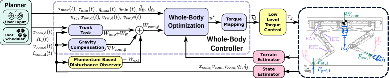
Figure 2.1: Overview of the whole-body controller as part of our locomotion framework. The dashed black box (cartouche) presents an overview of the robot’s joints, feet and generated wrenches and forces. LH, LF, RH and RF are Left-Hind, Left-Front, Right-Hind and Righ-Front legs, respectively. HAA, HFE and KFE are Hip Abduction/Adduction, Hip Flexion/Extension and Knee Flexion/Extension, respectively.

In our previous work [34], the locomotion controller was designed for quasi-static motions using only the robot’s centroidal dynamics. Under that assumption, we noticed that during dynamic motions, the effect of the leg dynamics no longer negligible; and thus, it becomes necessary to abandon the quasi-static assumption to achieve good tracking. Second, since the robot is constantly interacting with the environment (especially during walking and running), it is crucial to ensure a compliant and passive interaction. For these reasons, in this paper, we improve our previous work [34] by implementing a passivity based WBC that incorporates the full robot dynamics and interacts compliantly with the environment, while satisfying the kinematic and torque limits. Our WBC implementation is capable of achieving faster dynamic motions than our previous work. We also integrate terrain mapping and state estimation on-board and present some practical implementation details gained from the experience with the real platform.

Contributions: In this paper, we mainly present experimental contributions in which we demonstrate the effectiveness of the controller both in simulation and experiments on Hydraulically actuated Quadruped (HyQ). Compared to previous work on passivity-based WBC [29, 33], in which experiments were conducted on the robot while standing (not walking or running), we tested our controller on HyQ during crawling and trotting. Similar to the recent successful work of [26] and [40] in quadrupedal locomotion over rough terrain, we used similar terrain templates to present experiments of our passive WBC on HyQ using multiple gaits over slopes and rough terrain of different heights.

The rest of this paper is structured as follows: In Section 2.2 we present the detailed formulation and design of our WBC followed by its passivity analysis in Section 2.3. Section 2.4 presents further crucial implementation details. Finally we present our simulation and experimental results in Section 2.5 followed by our conclusions in Section 2.6.

2.2  Whole-Body Controller (WBC)

In this section we present and formulate our WBC. Figure 2.1 depicts the main components of our locomotion framework. Given high-level user velocity commands, the planner generates a reference motion online [41] or offline [25], and provides it to the WBC. Such references include the desired trajectories for CoM, trunk orientation and swing legs. The state estimator supplies the controller with an estimate of the actual state of the robot, by fusing leg odometry, inertial sensing, visual odometry and LIDAR while, the terrain estimator, provides an estimate of the terrain inclination (i.e. surface normal). Finally, there is a momentum-based observer that estimates external disturbances [41] and a lower-level torque controller. The goal of the designed WBC is to keep the quadruped robot balanced (during running, walking or standing) while interacting passively with the environment. The motion tasks of a quadruped robot can be categorized into a trunk task and a swing task. The trunk task regulates the position of the CoM and the orientation of the trunk and is achieved by implementing a Cartesian-based impedance controller with a feed-forward term. The swing task regulates the swing foot trajectory in order to place it in the desired location while achieving enough clearance from the terrain. Similar to the trunk task, the swing task is achieved by implementing a Cartesian-based impedance controller with a feed-forward term. The WBC realizes these tasks by computing the optimal generalized accelerations and contact forces [27] via QP and mapping them to the desired joint torques while taking into account the full dynamics of the robot, the properties of the terrain (friction constraints), the unilaterality of the contacts (e.g. the legs can only push and not pull) (unilateral constraints), and the actuator’s torque/kinematic limits. The desired torques, will be sent to the lower-level (torque) controller.

2.2.1   Robot Model

For a legged robot with $n$ DoFs and $c$ feet, the forward kinematics of each foot is defined by $n_{{a}}$ coordinates. The total dimension of the feet operational space is $n_{{f}}=n_{{a}}c$. This can be separated into stance ($n_{\mathrm{st}}=n_{{a}}c_{\mathrm{st}}$) and swing feet ($n_{\mathrm{sw}}=n_{{a}}c_{\mathrm{sw}}$). Since we are interested in regulating the position of the CoM, we formulate the dynamics in terms of the CoM, using its velocity rather than the base velocity [33]. Assuming that all the external forces are exerted on the stance feet, we write the equation of motion that describes the full dynamics of the robot as:

$$\underbrace{\begin{bmatrix}M_{\mathrm{com}}&0_{6\times n}\\ 0_{n\times 6}&\bar{M}_{j}\end{bmatrix}}_{M(q)}\!\!\underbrace{\begin{bmatrix}\dot{v}_{\mathrm{com}}\\ \ddot{q}_{j}\end{bmatrix}}_{\ddot{q}}\!+\!\underbrace{\begin{bmatrix}h_{com}\\ \bar{h}_{j}\end{bmatrix}}_{h}\!=\!\begin{bmatrix}0_{6\times n}\\ \tau_{j}\end{bmatrix}+\underbrace{\begin{bmatrix}J_{\mathrm{st,com}}^{T}\\ J_{\mathrm{st,j}}^{T}\end{bmatrix}}_{J_{\mathrm{st}}(q)^{T}}F_{\mathrm{grf}}$$ (2.1)

where the first 6 rows represent the (un-actuated) floating base part and the remaining $n$ rows represent the actuated part. $q\in SE(3)\times\mathbb{R}^{n}$ represents the pose of the whole floating-base system while $\dot{q}=\begin{bmatrix}v_{\mathrm{com}}^{T}&\dot{q}_{j}^{T}\end{bmatrix}^{T}\in\mathbb{R}^{6+n}$ and $\ddot{q}=[\dot{v}_{\mathrm{com}}^{T}\ \ddot{q}_{j}^{T}]^{T}\in\mathbb{R}^{6+n}$ are the vectors of generalized velocities and accelerations, respectively. $v_{\mathrm{com}}=[\dot{x}_{\mathrm{com}}^{T}\ \omega_{b}^{T}]^{T}$ $\in\mathbb{R}^{6}$ and $\dot{v}_{\mathrm{com}}=[\ddot{x}_{\mathrm{com}}^{T}\ \dot{\omega}_{b}^{T}]^{T}$ $\in\mathbb{R}^{6}$ are the spatial velocity and acceleration of the floating-base expressed at the CoM. $M(q)\in\mathbb{R}^{(6+n)\times(6+n)}$ is the inertia matrix, where $M_{\mathrm{com}}(q)$ $\in\mathbb{R}^{6\times 6}$ is the composite rigid body inertia matrix of the robot expressed at the CoM. $h\in\mathbb{R}^{6+n}$ is the force vector that accounts for Coriolis, centrifugal, and gravitational forces. $\tau\in\mathbb{R}^{n}$ are the actuated joint torques while $F_{\mathrm{grf}}\in\mathbb{R}^{n_{\mathrm{st}}}$ is the vector of Ground Reaction Forces (GRFs) (contact forces). In this context, the floating base Jacobian $J$ $\in\mathbb{R}^{n_{\mathrm{f}}\times(6+n)}$ is separated into swing Jacobian $J_{\mathrm{sw}}$ $\in\mathbb{R}^{n_{\mathrm{sw}}\times(6+n)}$ and stance Jacobian $J_{\mathrm{st}}$ $\in\mathbb{R}^{n_{\mathrm{st}}\times(6+n)}$ which could be further expanded into $J_{\mathrm{st,com}}$ $\in\mathbb{R}^{n_{\mathrm{st}}\times 6}$, $J_{\mathrm{st,j}}$ $\in\mathbb{R}^{n_{\mathrm{st}}\times n}$, $J_{\mathrm{sw,com}}$ $\in\mathbb{R}^{n_{\mathrm{sw}}\times 6}$ and $J_{\mathrm{sw,j}}$ $\in\mathbb{R}^{n_{\mathrm{sw}}\times n}$. The operator $\bar{[\cdot]}$ denotes the matrices/vectors recomputed after the coordinate transform to the CoM [38]. Following the sign convention in Fig. 2.1, recalling the first 6 rows in (2.1), and by defining the gravito-inertial CoM wrench as $W_{\mathrm{com}}=M_{\mathrm{com}}\dot{v}_{\mathrm{com}}+h_{com}$ $\in\mathbb{R}^{6}$, we can write the floating-base dynamics as:

$$W_{\mathrm{com}}=J_{\mathrm{st,com}}^{T}F_{\mathrm{grf}}$$ (2.2)

such that $J_{\mathrm{st,com}}^{T}$ maps $F_{\mathrm{grf}}$ to the CoM wrench space.

The feet velocities $v=[v_{\mathrm{st}}^{T}\ v_{\mathrm{sw}}^{T}]^{T}$ $\in\mathbb{R}^{n_{\mathrm{f}}}$ could be separated into stance $v_{\mathrm{st}}$ $\in\mathbb{R}^{n_{\mathrm{st}}}$ and swing $v_{\mathrm{sw}}$ $\in\mathbb{R}^{n_{\mathrm{sw}}}$ feet velocities. The mapping between $v$ and the generalized velocities $\dot{q}$ is:

$$v = J\dot{q}$$ (2.3a)

$$v=\begin{bmatrix}J_{\mathrm{com}}&J_{{j}}\end{bmatrix}\begin{bmatrix}v_{\mathrm{com}}\\ \dot{q}_{j}\end{bmatrix} = J_{\mathrm{com}}v_{\mathrm{com}}+J_{{j}}\dot{q}_{j}$$ (2.3b)

such that $J_{\mathrm{com}}$ $\in\mathbb{R}^{n_{\mathrm{f}}\times 6}$ and $J_{{j}}$ $\in\mathbb{R}^{n_{\mathrm{f}}\times n}$. Similar to the feet velocities, we split the feet force vector $F=[F_{\mathrm{st}}^{T}\ F_{\mathrm{sw}}^{T}]^{T}$ $\in\mathbb{R}^{n_{\mathrm{f}}}$, into $F_{\mathrm{st}}$ $\in\mathbb{R}^{n_{\mathrm{st}}}$ and $F_{\mathrm{sw}}$ $\in\mathbb{R}^{n_{\mathrm{sw}}}$.

Assumption 2.1

The robot is walking over rigid terrain in which the stance feet do not move (i.e., $v_{\mathrm{st}}=\dot{v}_{\mathrm{st}}=0$).

2.2.2   Trunk and Swing Leg Control Tasks

To compliantly achieve a desired motion of the trunk, we define the desired wrench at the CoM $W_{\mathrm{com,d}}$ using the following: 1) a Cartesian impedance at the CoM $W_{\mathrm{imp}}$ that is represented by a stiffness term ($\nabla V_{\mathrm{com,K}}=K_{\mathrm{com}}\Delta x_{\mathrm{com}}$) with positive definite stiffness matrix $K_{\mathrm{com}}\in R^{6\times 6}$ and a damping term ($D_{\mathrm{com}}\Delta v_{\mathrm{com}}$) with positive definite damping matrix $D_{\mathrm{com}}\in R^{6\times 6}$, 2) a virtual gravitational potential gradient to render gravity compensation $(\nabla V_{\mathrm{com,\bar{g}}}=mg)$, 3) a feedforward term to improve tracking ($W_{\mathrm{ff}}=M_{\mathrm{com}}\dot{v}_{\mathrm{com,d}}$) and a compensation term for external disturbances $-W_{\mathrm{ext}}$ [41]:

$$W_{\mathrm{com,d}} = W_{\mathrm{imp}}+\nabla V_{\mathrm{com,\bar{g}}}+W_{\mathrm{ff}}-W_{\mathrm{ext}}$$ (2.4a)

$$W_{\mathrm{imp}} = \nabla V_{\mathrm{com,K}}+D_{\mathrm{com}}\Delta v_{\mathrm{com}}$$ (2.4b)

such that $\Delta x_{\mathrm{com}}=x_{\mathrm{com,d}}-x_{\mathrm{com}}$, $\Delta v_{\mathrm{com}}=v_{\mathrm{com,d}}-v_{\mathrm{com}}$ are the tracking errors $\in\mathbb{R}^{6}$ of the position and velocity, respectively.

Similarly, the tracking of the swing task is obtained by the virtual force $F_{\mathrm{sw,d}}\in\mathbb{R}^{n_{\mathrm{sw}}}$. This is generated by 1) a Cartesian impedance at the swing foot that is represented by a stiffness term ($\nabla V_{\mathrm{sw}}=K_{\mathrm{sw}}\Delta x_{\mathrm{sw}}$) with positive definite stiffness matrix $K_{\mathrm{sw}}\in R^{n_{\mathrm{sw}}\times n_{\mathrm{sw}}}$ and a damping term ($D_{\mathrm{sw}}\Delta v_{\mathrm{sw}}$) with positive definite damping matrix $D_{\mathrm{sw}}\in R^{n_{\mathrm{sw}}\times n_{\mathrm{sw}}}$, and 2) a feedforward term to improve tracking ($F_{\mathrm{sw,ff}}=M_{\mathrm{sw}}\dot{v}_{\mathrm{sw,ff}}$):

$$F_{\mathrm{sw,d}} = \nabla V_{\mathrm{sw}}+D_{\mathrm{sw}}\Delta v_{\mathrm{sw}}+F_{\mathrm{sw,ff}}$$ (2.5)

such that $\Delta x_{\mathrm{sw}}=x_{\mathrm{sw,d}}-x_{\mathrm{sw}}$ and $\Delta v_{\mathrm{sw}}=v_{\mathrm{sw,d}}-v_{\mathrm{sw}}$ are the tracking errors of the swing feet positions and velocities respectively. Alternatively, it is possible to write this task at the acceleration level, with the difference that the gains $\mathrm{K}_{\mathrm{sw}}$ and $\mathrm{D}_{\mathrm{sw}}$ have no physical meaning:

$$\dot{v}_{\mathrm{sw,d}}=\dot{v}_{\mathrm{sw,ff}}+\mathrm{K}_{\mathrm{sw}}\Delta x_{\mathrm{sw}}+\mathrm{D}_{\mathrm{sw}}\Delta v_{\mathrm{sw}}$$ (2.6)

2.2.3   Optimization

To fulfill the motion tasks in Section 2.2.2 and to distribute the load on the stance feet, while respecting the mentioned constraints, we formulate the QP:

$$\underset{u=[\ddot{q}^{T}\hskip 5.69046ptF_{\mathrm{grf}}^{T}]^{T}}{\min}\|W_{\mathrm{com}}-W_{\mathrm{com,d}}\|^{2}_{Q}+\|u\|^{2}_{R}$$ (2.7a)

$$\text{s.t.}\hskip 14.22636pt\quad Au=b$$ (2.7b)

$$\underline{d}<Cu<\bar{d}$$ (2.7c)

such that our decision variables $u=[\ddot{q}^{T}\ F_{\mathrm{grf}}^{T}]^{T}\in\mathbb{R}^{6+n+n_{\mathrm{st}}}$ are the generalized accelerations $\ddot{q}$ and the contact forces $F_{\mathrm{grf}}$. The cost function (2.7a) is designed to minimize the trunk task and to regularize the solution. The equality constraints (2.7b) encode dynamic consistency, stance constraints and swing tasks. The inequality constraints (2.7c) encode friction constraints, joint kinematic and torque limits. All constraints are stacked in the matrix $A^{T}=\begin{bmatrix}A_{p}^{T}&A_{\mathrm{st}}^{T}&A_{\mathrm{sw}}^{T}\end{bmatrix}$ and $C^{T}=\begin{bmatrix}C_{\mathrm{fr}}^{T}&C_{j}^{T}&C^{T}_{\tau}\end{bmatrix}$ and detailed in the following sections.

2.2.3.1   Cost

The first term of the cost in (2.7a) represents the tracking error between the actual $W_{\mathrm{com}}$ and the desired $W_{\mathrm{com,d}}$ CoM wrenches from (2.2) and (2.4a) respectively. Since $W_{\mathrm{com}}$ is not a decision variable, we compute it from the contact forces (see (2.2)) and re-write $\|W_{\mathrm{com}}-W_{\mathrm{com,d}}\|_{Q}^{2}$ in the form of $\|Gu-g_{0}\|_{Q}^{2}$ with:

$$G=\begin{bmatrix}0_{6\times(6+n)}&J^{T}_{\mathrm{st,com}}\end{bmatrix},\quad g_{0}=W_{\mathrm{com,d}}$$ (2.8)

2.2.3.2   Physical consistency

To enforce physical consistency between $F_{\mathrm{grf}}$ and $\ddot{q}$, we impose the dynamics of the unactuated part of the robot (the trunk dynamics in (2.2)) as an equality constraint:

$$A_{p}=\begin{bmatrix}M_{\mathrm{com}}&0_{6\times n}&-J^{T}_{\mathrm{st,com}}\end{bmatrix},\quad b_{p}=-h_{com}$$ (2.9)

2.2.3.3   Stance condition

We can encode the stance feet constraints by re-writing them at the acceleration level in order to be compatible with the decision variables. Since $v_{\mathrm{st}}=J_{\mathrm{st}}\dot{q}$, differentiating once in time, yields to $\dot{v}_{\mathrm{st}}=J_{\mathrm{st}}\ddot{q}+\dot{J}_{\mathrm{st}}\dot{q}$. Recalling Assumption 2.1 yields $J_{\mathrm{st}}\ddot{q}+\dot{J}_{\mathrm{st}}\dot{q}=0$ which is encoded as:

$$A_{\mathrm{st}}=\begin{bmatrix}J_{\mathrm{st}}&0_{n_{\mathrm{st}}\times n_{\mathrm{st}}}\end{bmatrix},\quad b_{\mathrm{st}}=-\dot{J}_{\mathrm{st}}\dot{q}$$ (2.10)

such that $\dot{J}_{\mathrm{st}}$ is the time derivative of $J_{\mathrm{st}}$. For numerical precision, we compute the product $\dot{J}_{\mathrm{st}}\dot{q}$ using spatial algebra.

2.2.3.4   Swing task

Similar to Section 2.2.3.3, we can encode the swing task directly as an equality constraint, i.e. by enforcing the swing feet to follow a desired swing acceleration $\dot{v}_{\mathrm{sw}}(q)=\dot{v}_{\mathrm{sw,d}}\in\mathbb{R}^{n_{\mathrm{sw}}}$ yielding:

$$J_{\mathrm{sw}}\ddot{q}+\dot{J}_{\mathrm{sw}}\dot{q}=\dot{v}_{{\mathrm{sw,d}}}$$ (2.11)

that in matrix form becomes:

$$A_{\mathrm{sw}}=\begin{bmatrix}J_{\mathrm{sw}}&0_{n_{\mathrm{sw}}\times n_{\mathrm{st}}}\end{bmatrix},\quad b_{\mathrm{sw}}=\dot{v}_{{\mathrm{sw,d}}}-\dot{J}_{\mathrm{sw}}\dot{q}$$ (2.12)

where we computed $\dot{v}_{{\mathrm{sw,d}}}$ as in (2.6). Note that this implementation is analogous to the trunk task in Section 2.2.2. The difference is that this implementation is at the acceleration level while the other is at the force level. However, without any loss of generality, the formulation (2.5) could also be used. In Section 2.4.2 we incorporate slacks in the optimization to allow temporary violation of the swing tasks (e.g. useful when the kinematic limits are reached).

2.2.3.5   Friction cone constraints

To avoid slippage and obtain a smooth loading/unloading of the legs, we incorporate friction/unilaterality constraints. For that, we ensure that the contact forces lie inside the friction cones and their normal components stay within some user-defined values (i.e. maximum and minimum force magnitudes). We approximate the friction cones with square pyramids to express them with linear constraints. The fact that the ground contacts are unilateral, can be naturally encoded by setting an “almost-zero” lower bound on the normal component, while the upper bound allows us to regulate the amount of “loading” for each leg. We define the friction inequality constraints as:

$$\underline{d}_{\mathrm{fr}}<C_{\mathrm{fr}}u<\bar{d}_{\mathrm{fr}},\quad C_{\mathrm{fr}}=\begin{bmatrix}0_{p\times(6+n)}&F_{\mathrm{fr}}\end{bmatrix}$$ (2.13)

with:

$$F_{\mathrm{fr}}=\begin{bmatrix}F_{0}&\dots&0\\ \vdots&\ddots&\vdots\\ 0&\dots&F_{c}\end{bmatrix},\ \ \ \underline{d}_{\mathrm{fr}}=\begin{bmatrix}\underline{f}_{0}\\ \vdots\\ \underline{f}_{c}\end{bmatrix},\ \ \ \bar{d}_{\mathrm{fr}}=\begin{bmatrix}\bar{f}_{0}\\ \vdots\\ \bar{f}_{c}\end{bmatrix}$$ (2.14)

where $F_{\mathrm{fr}}\in\mathbb{R}^{p\times n_{\mathrm{st}}}$ is a block diagonal matrix that encodes the friction cone boundaries and select the normals, for each stance leg and $\underline{d}_{\mathrm{fr}},\bar{d}_{\mathrm{fr}}\in\mathbb{R}^{p}$ are the lower/upper bounds respectively. For the detailed implementation of the friction constraints refer to [34].

2.2.3.6   Torque limits

We notice that the torques be obtained from the decision variables since they can be expressed as a bi-linear function of $\ddot{q}_{j}$ and $F_{\mathrm{grf}}$. Therefore, the constraint on the joint torques (i.e., the actuation limits $\tau_{\min}<\tau_{j}<\tau_{\max}$) can be encoded by exploiting the actuated part of the dynamics (2.1):

$$\underline{d}_{\tau}<C_{\tau}u<\bar{d}_{\tau},\quad C_{\tau}=\begin{bmatrix}0_{n\times 6}&\bar{M}_{j}&-J_{\mathrm{st,j}}^{T}\end{bmatrix}$$ (2.15)

$$\underline{d}_{\tau}=-\bar{h}_{j}+\tau_{\min}(q_{j}),\quad\bar{d}_{\tau}=-\bar{h}_{j}+\tau_{\max}(q_{j})$$

where $\tau_{\min}(q_{j}),\tau_{\max}(q_{j})\in\mathbb{R}^{n}$ are the lower/upper bounds on the torques. In the case of our quadruped robot, these bounds must be recomputed at each control loop because they depend on the joint positions. This is due to the presence of linkages on the sagittal joints (HFE and KFE), that set a joint-dependent profile on the maximum torque (non-linear in the joint range).

2.2.3.7   Joint kinematic limits

We enforce joint kinematic constraints as function of the joint accelerations (i.e. $\ddot{q}_{j_{\min}}<\ddot{q}_{j}<\ddot{q}_{j_{\max}}$). We select them via the matrix $C_{j}$:

$$\underline{d}_{j}<C_{j}u<\bar{d}_{j},\quad{C}_{j}=\begin{bmatrix}0_{n\times 6}&I_{n\times n}&0_{n\times n_{\mathrm{st}}}\end{bmatrix}$$ (2.16)

$$\underline{d}_{j}=\ddot{q}_{j_{\min}}(q_{j}),\quad\quad\bar{d}_{j}=\ddot{q}_{j_{\max}}(q_{j})$$ (2.17)

such that $\ddot{q}_{j_{\min}}(q_{j})$ and $\ddot{q}_{j_{\max}}(q_{j})$ are the upper/lower bounds on accelerations. These bounds should be recomputed at each control loop. They are set in order to make the joint to reach the end-stop at a zero velocity in a time interval $\Delta t=10dt$, where $dt$ is the loop duration. For instance, if the joint is at a distance $q_{j_{\max}}-q_{j}$ from the end-stop with a velocity $\dot{q}_{j}$, the deceleration to cover this distance in a time interval $\Delta t$, and approach the end-stop with zero velocity, will be:

$$\ddot{q}_{j_{\min,\max}}=-\frac{2}{\Delta t^{2}}(q_{j_{\min,\max}}-q_{j}-\Delta t\,\dot{q}_{j})$$ (2.18)

2.2.4   Torque computation

We map the optimal solution $u^{*}=\begin{bmatrix}\ddot{q}^{*}&F_{\mathrm{grf}}^{*}\end{bmatrix}$ obtained by solving (2.7), into desired joint torques $\tau_{d}^{*}\in\mathbb{R}^{n}$ using the actuated part of the dynamics equation of the robot as:

$$\tau_{d}^{*}=\bar{M}_{j}\ddot{q_{j}}^{*}+\bar{h}_{j}-J_{\mathrm{st,j}}^{T}F_{\mathrm{grf}}^{*}$$ (2.19)

2.3  Passivity Analysis

The overall system consists of the WBC, the robot and the environment. This system is said to be passive if all these components, and their interconnections are passive [37]. If the robot and the environment are passive, and the controller is proven to be passive, then the overall system is passive [42]. A system (with input $u$ and output $y$) is said to be passive if there exists a storage function $S$ that is bounded from below and its derivative $\dot{S}$ is less than or equal to its supply rate ($s=y^{T}u$). In this context, we define the total energy stored in the controller to be the candidate storage function for the controller $S=V$. The rest of this section is devoted to analyze the passivity of the overall system.

Assumption 2.2

A feasible solution exists for the QP in (2.7) in which the motion tasks are achieved. Moreover, we do not consider the feed-forward terms in (2.4a) and (2.5) leaving this to future developments.

We start by defining the velocity error at the joints and at the stance feet to be $\Delta\dot{q}_{j}=\dot{q}_{j,d}-\dot{q}_{j}$, and $\Delta v_{\mathrm{st}}=v_{\mathrm{st,d}}-v_{\mathrm{st}}$, respectively. We also define the desired feet forces $F_{\mathrm{d}}=[F_{\mathrm{st,d}}^{T}\ F_{\mathrm{sw,d}}^{T}]^{T}$ such that, by following the sign convention in Fig. 2.1, the mapping between $F_{\mathrm{d}}$ and $W_{\mathrm{com,d}}$ is expressed as:

$$W_{\mathrm{com,d}}=-J_{\mathrm{com}}^{T}F_{\mathrm{d}},$$ (2.20)

while mapping between $F_{d}$ and $\tau_{j}$ is expressed as

$$\tau = J_{{j}}^{T}F_{d}.$$ (2.21)

By defining $\nabla V_{\mathrm{com}}=\nabla V_{\mathrm{com,K}}+\nabla V_{\mathrm{com,\bar{g}}}$ and recalling (2.20), we rewrite (2.4a) under Assumption 2.2 as:

$$\nabla V_{\mathrm{com}} = W_{\mathrm{com,d}}-D_{\mathrm{com}}\Delta v_{\mathrm{com}}$$ (2.22a)

$$= -J_{\mathrm{com}}^{T}F_{\mathrm{d}}-D_{\mathrm{com}}\Delta v_{\mathrm{com}}.$$ (2.22b)

2.3.1   Analysis

The overall energy in the whole-body controller is the one stored in the virtual impedance at the CoM and the potential energy due to gravity compensation ($V_{\mathrm{com}}$), and the energy stored in the virtual impedances at the swing feet ($V_{\mathrm{sw}}$):

$$V=V_{\mathrm{com}}+V_{\mathrm{sw}}.$$ (2.23)

The time derivatives are:

$$\dot{V}=\dot{V}_{\mathrm{com}}+\dot{V}_{\mathrm{sw}}=\Delta v_{\mathrm{com}}^{T}\nabla V_{\mathrm{com}}+\Delta v_{\mathrm{sw}}^{T}\nabla V_{\mathrm{sw}}.$$ (2.24)

Recalling (2.5) and (2.22b), (2.24) yields:

$$\dot{V} = \Delta v_{\mathrm{com}}^{T}(-J_{\mathrm{com}}^{T}F_{\mathrm{d}}-D_{\mathrm{com}}\Delta v_{\mathrm{com}})+$$ (2.25)

$$\Delta v_{\mathrm{sw}}^{T}(F_{\mathrm{sw,d}}-D_{\mathrm{sw}}\Delta v_{\mathrm{sw}})).$$

We regroup $\dot{V}$ in terms of the non-damping terms $\dot{V}_{1}$ and damping terms $\dot{V}_{2}$ yielding:

$$\dot{V_{1}} = -\Delta v_{\mathrm{com}}^{T}J_{\mathrm{com}}^{T}F_{\mathrm{d}}+\Delta v_{\mathrm{sw}}^{T}F_{\mathrm{sw,d}}$$ (2.26a)

$$\dot{V_{2}} = -\Delta v_{\mathrm{com}}^{T}D_{\mathrm{com}}\Delta v_{\mathrm{com}}-\Delta v_{\mathrm{sw}}^{T}D_{\mathrm{sw}}\Delta v_{\mathrm{sw}}.$$ (2.26b)

We rewrite (2.3b) in terms of $\Delta v_{\mathrm{com}}$, $\Delta v$ and $\Delta\dot{q}_{\mathrm{j}}$ as:

$$\Delta v = J_{\mathrm{com}}\Delta v_{\mathrm{com}}+J_{\mathrm{j}}\Delta\dot{q}_{\mathrm{j}}$$ (2.27a)

$$\Delta v_{\mathrm{com}}^{T}J_{\mathrm{com}}^{T} = -\Delta\dot{q}_{\mathrm{j}}^{T}J_{\mathrm{j}}^{T}+\Delta v^{T}.$$ (2.27b)

Plugging, (2.27b) in (2.26a) yields:

$$\dot{V_{1}} = \Delta\dot{q}_{\mathrm{j}}^{T}J_{\mathrm{j}}^{T}F_{\mathrm{d}}-\Delta v^{T}F_{\mathrm{d}}+\Delta v_{\mathrm{sw}}^{T}F_{\mathrm{sw,d}}$$ (2.28a)

$$= \Delta\dot{q}_{\mathrm{j}}^{T}J_{\mathrm{j}}^{T}F_{\mathrm{d}}-\Delta v_{\mathrm{st}}^{T}F_{\mathrm{st,d}}.$$ (2.28b)

Plugging (2.21) and into (2.28b) yields:

$$\dot{V_{1}} = \Delta\dot{q}_{\mathrm{j}}^{T}\tau-\Delta v_{\mathrm{st}}^{T}F_{\mathrm{st,d}}.$$ (2.29)

Under Assumption 2.1, (2.29) yields:

$$\dot{V_{1}} = \Delta\dot{q}_{\mathrm{j}}^{T}\tau.$$ (2.30)

Thus, $\dot{V}$ could be rewritten as:

$$\dot{V}=\Delta\dot{q}_{\mathrm{j}}^{T}\tau-\Delta v_{\mathrm{com}}^{T}D_{\mathrm{com}}\Delta v_{\mathrm{com}}-\Delta v_{\mathrm{sw}}^{T}D_{\mathrm{sw}}\Delta v_{\mathrm{sw}}.$$ (2.31)

2.3.2   Proof

Under Assumption 2.2, the designed WBC is an impedance control with gravity compensation that, similar to a PD+ [39], defines a map of $(\dot{q}_{\mathrm{j}}-\dot{q}_{\mathrm{j,d}})\mapsto-\tau$. This controller is passive if $V$ is bounded from below and $\dot{V}\leq\Delta\dot{q}_{\mathrm{j}}^{T}\tau$. Since $V$ consists of positive definite potentials that resemble Cartesian stiffnesses at the CoM and the swing leg(s), and under the assumption the gravitational potential is bounded from below (see [43]), $V$ is also bounded from below. Additionally, recalling (2.31) proves that the controller is indeed passive; thus, the overall system is passive.

2.4  Implementation Details

This section describes some pragmatic details that we found crucial in the implementation on the real platform.

2.4.1   Stance task

Uncertainties in estimating the terrain’s normal direction and friction coefficient could result in slippage. This can lead to considerable motion of the stance feet with possible loss of stability. To avoid this, a joint impedance feedback loop could be run in parallel to the WBC, at the price of losing the capability of optimizing the GRFs. A cleaner solution is to incorporate, in the optimization, Cartesian impedances specifically designed to keep the relative distance among the stance feet constant (we denote it stance task).

The stance task has an influence only when there is an anomalous motion in the stance feet, retaining the possibility to freely optimize for GRFs in normal situations. This can be achieved by re-formulating the stance condition in (2.10) as a desired stance feet acceleration $\dot{v}_{\mathrm{st,d}}$ as:

$$\dot{v}_{\mathrm{st,d}}=K_{\mathrm{st}}(\hat{x}_{\mathrm{st}}-x_{\mathrm{st}})-D_{\mathrm{st}}v_{\mathrm{st}}.$$ (2.32)

This term is added to $b_{st}$ (in (2.10)) as $b_{st}=-\dot{J}_{st}\dot{q}+\ddot{x}^{d}_{f_{st}}$ where $\hat{x}_{\mathrm{st}}$ is a sample of the foot position at the touchdown (expressed in the world frame).

2.4.2   Constraint Softening

Adding slack variables to an optimization problem is commonly done to avoid infeasible solutions, by allowing a certain degree of constraint violation. Infeasibility can occur when hard constraints are conflicting with each other, which can be the case in our QP. Hence, some of the equalities/inequalities in (2.7) should be relaxed if they are in conflict.

We decided not to introduce slacks in the torque constraints (Section 2.2.3.6) or the dynamics (Section 2.2.3.2) keeping them as hard constraints, since torque constraints and physical consistency should never be violated. On the other hand it is important to allow a certain level of relaxation for the swing tasks in Section 2.2.3.4 that could be violated if the joint kinematic limits are reached.

To relax the constraints of the swing task, first, we augment the decision variables $\tilde{u}=[u^{T}\ \epsilon^{T}]^{T}\in\mathbb{R}^{6+n+k+n_{sw}}$ with the vector of slack variables $\epsilon\in\mathbb{R}^{n_{sw}}$ where we introduce a slack variable for each direction of the swing tasks. Then, we replace the equality constraint $A_{sw}u+b_{sw}=0$ of the swing tasks, by two inequality constraints:

$$-\epsilon\leq A_{sw}\tilde{u} +b_{sw}\leq\epsilon$$

$$\epsilon \geq 0.$$ (2.33)

The first inequality in (2.4.2) restricts the solution to a bounded region around the original constraint while the second one ensures that the slack variables remain non-negative. To make sure that there is a constraint violation only when the constraints are conflicting, we minimize the norm of the slack vector adding a regularization term $\alpha\|\epsilon\|^{2}$ to (2.7a) with a high weight $\alpha$.

To reduce the computational complexity, we could have introduced a single slack for each swing task (rather than one for each direction). However, this could create coupling errors in the tracking. For instance, since the Hip Flexion-Extension (HFE) joint (see Fig. 2.1) mainly acts in the $XZ$ plane, if it reaches its joint limit, only that plane should be affected leaving the $Y$ direction unaffected. A single slack couples the three directions causing tracking errors also in the $Y$ direction. Conversely, using multiple slacks, only the directions the HFE acts upon, will be affected.

2.5  Results

In this section we validate the capabilities of the controller under various terrain conditions and locomotion gaits. The WBC and torque control loops run in real-time threads at 250 Hz and 1 kHz, respectively. We set the gains for the swing tasks to $K_{sw}=\mathrm{diag}({2000,2000,2000})$ and $D_{sw}=\mathrm{diag}({20,20,20})$, while for the trunk task we set $K_{x}=\mathrm{diag}({2000,2000,2000})$ $D_{x}=\mathrm{diag}({400,400,400})$ and $K_{\theta}=\mathrm{diag}({1000,1000,1000})$ $D_{\theta}=\mathrm{diag}({200,200,200})$. These values proved to be working in both simulation and real experiments. The results are collected in the accompanying video. Additionally, in experimental trials, we also included a low gain joint-space attractor (PD controller) for the swing task, since imprecise torque tracking of the knee joints (due to the low inertia) produce control instabilities in an operational space implementation (e.g. the one in Section 2.2.3.4).

2.5.1   Constraint Softening through Slack Variables

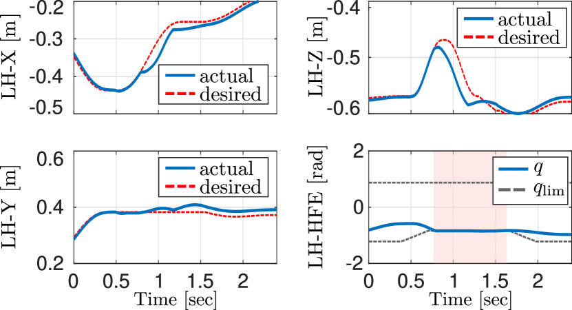
Figure 2.2: Simulation. Effect of (kinematic limits) slacks variables on foot tracking. The upper-left/right and bottom-left plots show the tracking of the desired foot position (LH leg) in $X$, $Y$ and $Z$, respectively. Bottom-right plot depicts the joint limits (black line) and the actual position (blue line) of the HFE joint. The red shaded area underlines that when the slack increases, the HFE joint is properly clamped.

In Fig. 2.2 we artificially incremented the lower limit of the LH-HFE joint. When the limit is hit, the bound on the joint acceleration (2.18) produces a desired torque command that stops its motion. This “naturally” clamps the actual joint position to the limit (bottom-left plot) and influences the foot tracking mainly along the $X$ and $Z$ directions.

Computational time: the solution of the QP takes between 90-110 $\mu s$ on a Intel i5 machine without the slacks variables. After augmenting the problem with the slack variables and its constraints, it increases 30 % on average (120-150 $\mu s$). However it still remains suitable for real-time implementation (250 $Hz$).

2.5.2   Friction Constraints and Bounded Slippage

We evaluated in simulation the controller performance against inaccurate friction coefficient estimates $\mu$, which define incorrectly the friction cone constraints in the WBC. In the accompanying video, we show an example where the robot crawls at 0.11 m/s on a slippery floor ($\mu=0.4$) while we set the friction coefficient to $\mu=1.0$ in the WBC, to emulate an estimation error. Simulation results support the fact that foot slippage remains bounded by the action of the stance task (Section 2.4.1). If we gradually correct $\mu$ the slippage events completely disappear; allowing an increase of forward velocity up to 0.16 m/s.

2.5.3   Torque Limits and Load Redistribution

We analyzed in simulation the effect of adding an artificial torque limit, in our WBC. This helps us to derive controllers that are robust against joint damages. Figure 2.3 shows a reduction of the torque limits down to 26 Nm in the Left-Front (LF)-KFE joint and the load redistribution among the other joints (HAA and HFE) of the LF leg. Indeed, while the KFE joint torque is clamped, the HFE is loaded more (lower plot). This load redistribution did not affect the trunk motion and it demonstrates how the controller exploits the torque redundancy by finding a new load distribution.

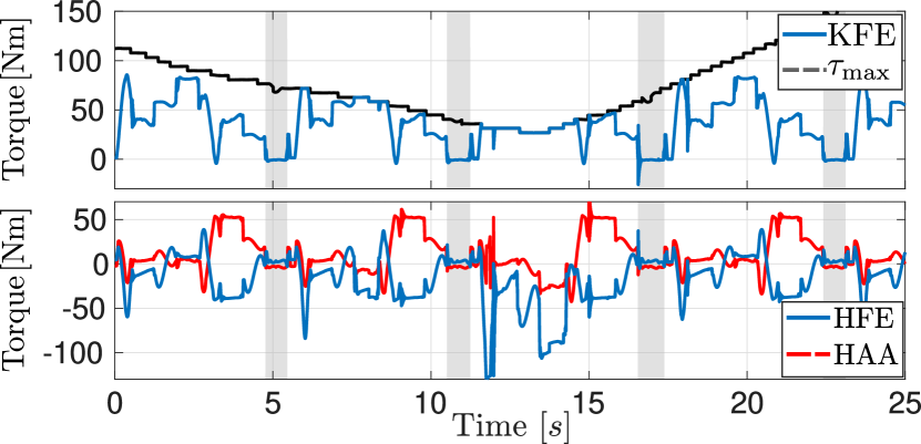
Figure 2.3: Simulation. Effect of introducing an artificial torque limit on the KFE joint of the LF leg during a typical crawl. The shaded area represents the swing phase of the leg while the unshaded part is the stance phase. We reduced the torque limit down to 26 Nm (black line, upper plot), and as a consequence, the HFE torque is increased by the controller (bottom plot).

We carried out also intensive experimental validation in various challenging terrains. Slopes increase the probability of reaching torque limits because of the more demanding kinematic configurations. Indeed, in Fig. 2.4, the robot reached three times the torque limits (red shaded areas). Crossing this terrain would not be possible without enforcing the torque limits as hard constraints.

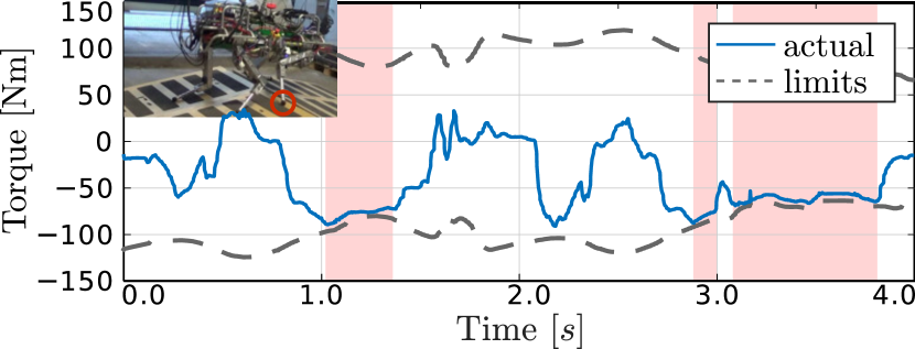
Figure 2.4: Real experiments. Reaching the torque limits on the RF-HFE joint while climbing up and down two ramps. The HyQ robot reached three times its torque limits (red shaded areas). The real torque (blue line) is tracking the desired one (not shown) computed from our whole-body controller while satisfying the joint limits (black line). The torque limits are time-varying due to the joint mechanism.

2.5.4   Different Torque Regularization Schemes

By setting different regularizations in (2.7a) [34], we can either choose to maximize the robustness to uncertainties in the friction parameters (e.g. GRFs closer to the friction cone normals) or to minimize the joint torques. In the latter case, for instance, we could encourage the controller to use a particular joint by increasing its corresponding weight. If we gradually increase the weight of the Knee Flexion-Extension (KFE) joints (see accompanying video), the effect of torque regularization becomes visible because the GRFs are no longer vertical. Indeed the GRFs start to point toward the knee axis in order to reduce its torque command.

2.5.5   Comparison with Previous Controller (Quasi-Static)

We compare our whole-body controller (dynamic) against a centroidal-based controller (quasi-static) [34]. As metric we use the $l^{2}$-norm for the linear $e_{x}$ and angular $e_{\theta}$ tracking errors of the trunk task. If we increase linearly the forward speed from 0.04 m/s to 0.15 m/s, the tracking error is reduced approximately by 50 % in comparison to the quasi-static controller (Fig. 2.5). This is due to the fact that our WBC computes both joint accelerations and contact forces, which allows a proper mapping of torque commands (inverse dynamics). Indeed this results in better accuracy in the execution of more dynamic motions.

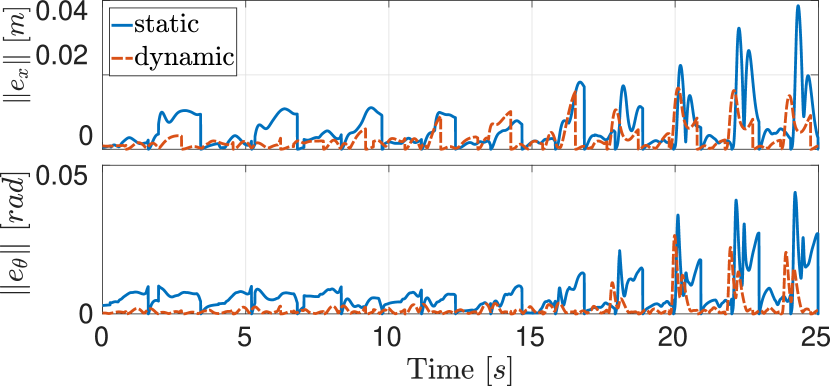
Figure 2.5: Simulation. Comparison of tracking errors for the trunk task of a quasi-static controller against our whole-body controller (dynamic). $l^{2}$-norms of linear and angular errors are shown in the top and bottom figures. Note that the errors are reset to zero at each step due to re-planning.

2.5.6   Disturbance Rejection against Unstable Foothold

We encoded compliance tracking of the CoM task through a virtual impedance. Friction cone constraints help to instantaneously keep the robot’s balance whenever a tracking error happens due to, for instance, an unstable foothold. Furthermore joint constraints (positions and torques) guarantee feasibility of the computed torque commands. Figure 2.6 shows how the controller compliantly tracks the desired CoM trajectory during an unstable footstep (a rolling stepping-stone) that occurs at $t=6.5$ s (experiments results from [44]). This creates tracking errors on the CoM height, yet, good tracking performance is kept for the horizontal CoM motion, due to the friction cone constraints that maintained the robot’s balance along the entire locomotion.

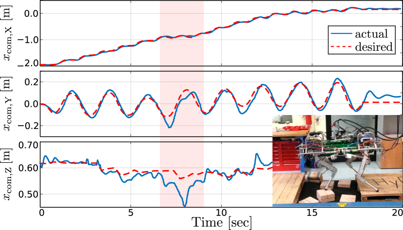
Figure 2.6: Real experiments. Disturbance rejection against unstable foothold that occurs when a stepping-stone rolled under the RF leg at $t=6.5$ s. The controller lost tracking of the CoM height, however, the friction cone constraints keep instantaneously the robot’s balance. Indeed a good tracking of the horizontal motion of the CoM is obtained. Note that the red shaded area depicts the moments of the disturbance rejection.

2.5.7   Locomotion over Slopes

These experiments have been performed with online terrain mapping [41]. Both the terrain mapping and the whole-body controller make use of a drift-free state estimation algorithm to obtain the body state. The friction cone constraints of the controller are described given the real terrain normals provided by an onboard mapping algorithm. The friction coefficient has been conservatively set to 0.7 for all the experiments. Figure 2.7 shows different snapshots of various challenging terrain used to evaluate our controller. The centroidal trajectory, gait and footholds are computed simultaneously as described in [25].

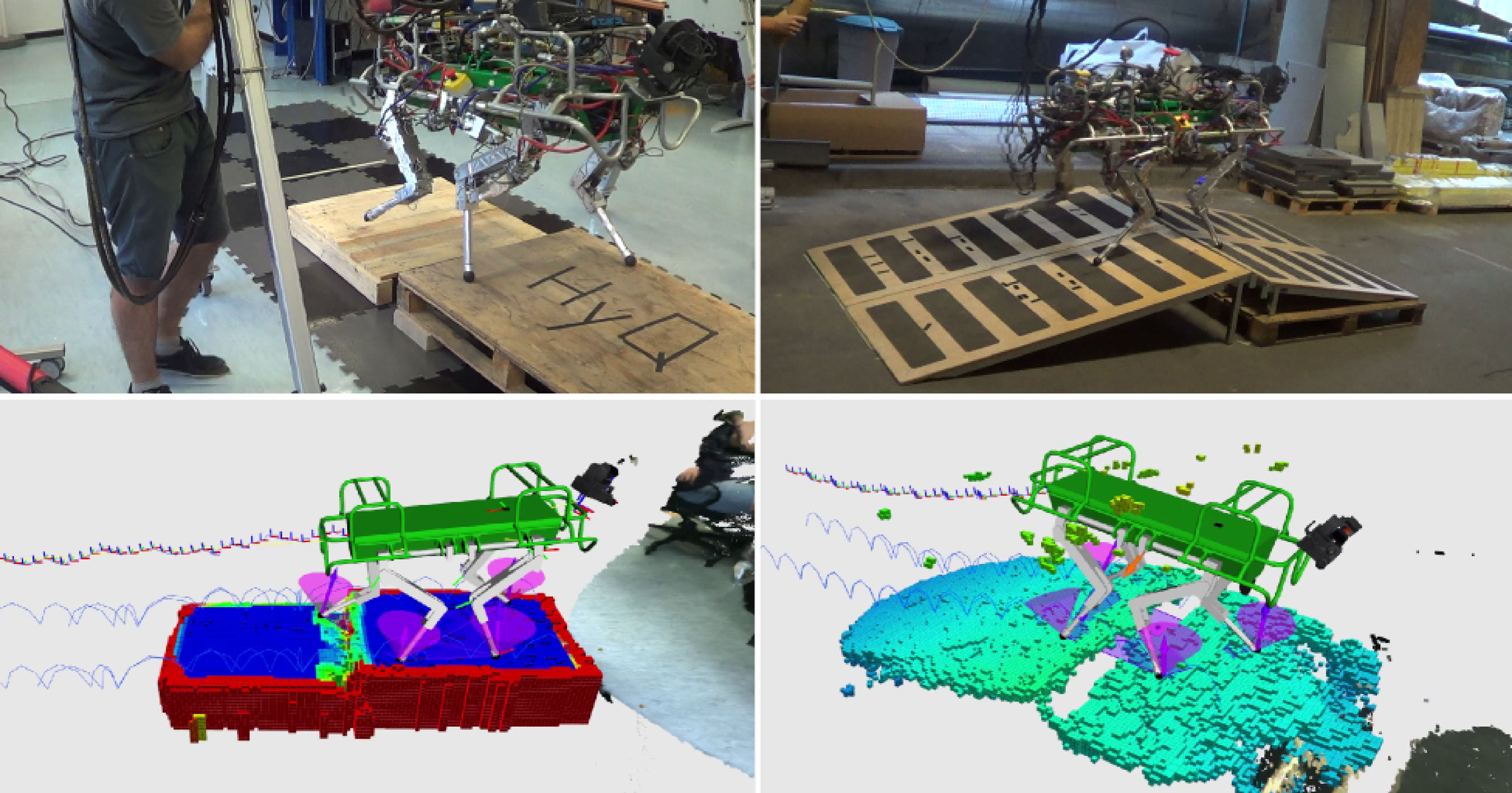
Figure 2.7: Snapshots of experimental trials to evaluate our whole-body control and the online terrain mapping. Left column: crossing a 22 cm gap with a 7 cm step. Right column: traversing two ramps with a 15 cm gap between them.

2.5.8   Tracking Performance with Different Gaits

The quadrupedal trotting gait is difficult to control because the robot uses only two legs at the time to achieve the tracking of the desired CoM motion and of the trunk orientation. Figure 2.8 depicts the roll and pitch tracking for climbing up a ramp during a trotting gait. Although a trot is an under-actuated gait, our controller can still track the desired orientation. Moreover, in these cases, the orientation error is always below 0.2 rad.

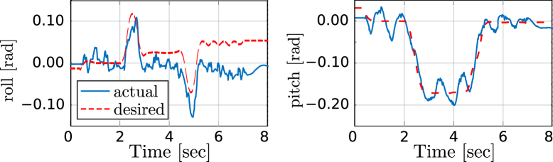
Figure 2.8: Real experiments. Roll and pitch tracking performance while climbing up a ramp with a trotting gait. Although there is under-actuation the controller can still track roll and pitch motions.

2.6  Conclusion

This paper presented an experimental validation of our passive WBC. Compared to our previous work [34], the presented WBC enables higher dynamic motions thanks to the use of the full dynamics of the robot. Although similar controllers have been proposed in the literature (e.g. [27, 29, 26]), we validated our locomotion controller on HyQ over a wide range of challenging terrain (slopes, gaps, stairs, etc.), using different gaits (crawl and trot). Additionally, we have analyzed the controller capabilities against 1) inaccurate friction coefficient estimation, 2) unstable footholds, 3) changes in the regularization scheme and 4) the load redistribution under restrictive torque limits. Extensive experimental results validated the controller performance together with the online terrain mapping and the state estimation. Moreover, we demonstrated experimentally the superiority of our WBC compared to a quasi-static control scheme [34].

Chapter 3  STANCE:
Locomotion Adaptation over Soft Terrain

Abstract. Whole-Body Control (WBC) has emerged as an important framework in locomotion control for legged robots. However, most WBC frameworks fail to generalize beyond rigid terrains. Legged locomotion over soft terrain is difficult due to the presence of unmodeled contact dynamics that WBCs do not account for. This introduces uncertainty in locomotion and affects the stability and performance of the system. In this paper, we propose a novel soft terrain adaptation algorithm called STANCE: Soft Terrain Adaptation and Compliance Estimation. STANCE consists of a WBC that exploits the knowledge of the terrain to generate an optimal solution that is contact consistent and an online terrain compliance estimator that provides the WBC with terrain knowledge. We validated STANCE both in simulation and experiment on the Hydraulically actuated Quadruped (HyQ) robot, and we compared it against the state of the art WBC. We demonstrated the capabilities of STANCE with multiple terrains of different compliances, aggressive maneuvers, different forward velocities, and external disturbances. STANCE allowed HyQ to adapt online to terrains with different compliances (rigid and soft) without pre-tuning. HyQ was able to successfully deal with the transition between different terrains and showed the ability to differentiate between compliances under each foot.

Accompanying Video. https://youtu.be/0BI4581DFjY

3.1  Introduction

Whole-Body Control (WBC) frameworks have achieved remarkable results in legged locomotion control [30, 45, 1]. Their main feature is that they use optimization techniques to solve the locomotion control problem. WBC can achieve multiple tasks in an optimal fashion by exploiting the robot’s full dynamics and reasoning about both the actuation constraints and the contact interaction. These tasks include balancing, interacting with the environment, and performing dynamic locomotion over a wide variety of terrains [1]. The tasks are executed at the robot’s end effectors, but can also be utilized for contacts anywhere on the robot’s body [35] or for a cooperative manipulation task between robots [36].

To date, most of the work done on WBC assumes that the ground is rigid (i.e., rigid contact consistent). However, if the robot traverses soft terrain (as shown in Fig. 3.1), the mismatch between the rigid assumption and the soft contact interaction can significantly affect the robot’s performance and locomotion stability. This mismatch is due to the unmodeled contact dynamics between the robot and the terrain. In fact, under the rigid ground assumption, the controller can generate instantaneous changes to the Ground Reaction Forces (GRFs). This is equivalent to thinking that the terrain will respond with an infinite bandwidth.

In order to robustly traverse a wide variety of terrains of different compliances, the WBC must become compliant contact consistent (c³). Namely, the WBC should be terrain-aware. That said, a more general WBC approach should be developed that can adapt online to the changes in the terrain compliance.

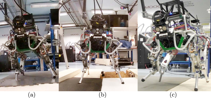
Figure 3.1: HyQ traversing multiple terrains of different compliances.

3.1.1   Related Work:
Soft Terrain Adaptation for Legged Robots

Locomotion over soft terrain can be tackled either from a control or a planning perspective. In the context of locomotion control, Henze et al. [29] presented the first experimental attempt using a WBC over soft terrain. Their WBC is based on the rigid ground assumption, but it allows for constraint relaxation. This allowed the humanoid robot TORO to adapt to a compliant surface. Their approach was further extended in [46] by dropping the rigid contact assumption and using an energy-tank approach. Despite balancing on compliant terrain, both approaches were only tested for one type of soft terrain when the robot was standing still.

Similarly, other works explicitly adapt to soft terrain by incorporating terrain knowledge (i.e., contact model) into their balancing controllers. For example, Azad et al. [47] proposed a momentum based controller for balancing on soft terrain by relying on a nonlinear soft contact model. Vasilopoulos et al. [48] proposed a similar hopping controller that models the terrain using a viscoplastic contact model. However, these approaches were only tested in simulation and for monopods.

In the context of locomotion planning, Grandia et al. [49] indirectly adapted to soft terrain by shaping the frequency of the cost function of their Model Predictive Control (MPC) formulation. By penalizing high frequencies, they generated optimal motion plans that respect the bandwidth limitations due to soft terrain. This approach was tested over three types of terrain compliances. However, it was not tested during transitions from one terrain to another. This approach showed an improvement in the performance of the quadruped robot in simulation and experiment. However, the authors did not offer the possibility to change their tuning parameters online. Thus, they were not able to adapt the locomotion strategy based on the compliance of the terrain.

In contrast to the aforementioned work, other approaches relax the rigid ground assumption (hard contact constraint) but not for soft terrain adaptation purposes. For instance, Kim et al. [50] implemented an approach to handle sudden changes in the rigid contact interaction. This approach relaxed the hard contact assumption in their WBC formulation by penalizing the contact interaction in the cost function rather than incorporating it as a hard constraint. For computational purposes, Neunert et al. [51] and Doshi et al. [52] proposed relaxing the rigid ground assumption. Neunert et al. used a soft contact model in their nonlinear MPC formulation to provide smooth gradients of the contact dynamics to be more efficiently solved by their gradient based solver. The soft contact model did not have a physical meaning and the contact parameters were empirically chosen. Doshi et al. proposed a similar approach which incorporates a slack variable that expands the feasibility region of the hard constraint.

Despite the improvement in performance of the legged robots over soft terrain in the aforementioned works, none of them offered the possibility to adapt to the terrain online. Most of the aforementioned works lack a general approach that can deal with multiple terrain compliances or with transitions between them. Perhaps, one noticeable work (to date) in online soft terrain adaptation was proposed by Chang et al. [53]. In that work, an iterative soft terrain adaptation approach was proposed. The approach relies on a non-parametric contact model that is simultaneously updated alongside an optimization based hopping controller. The approach was capable of iteratively learning the terrain interaction and supplying that knowledge to the optimal controller. However, because the learning module was exploiting Gaussian process regression, which is computationally expensive, the approach did not reach real-time performance and was only tested in simulation, for one leg, under one experimental condition (one terrain).

3.1.2   Related Work:
Contact Compliance Estimation in Robotics

For contact compliance estimation, we need to accurately model the contact dynamics and estimate the contact parameters online. In contact modeling, Alves et al. [54] presented a detailed overview of the types of parametric soft contact models used in the literature. In compliance estimation, Schindeler et al. [55] used a two stage polynomial identification approach to estimate the parameters of the Hunt and Crossley’s (HC) contact model online. Differently, Azad et al. [56] used a least square-based estimation algorithm and compared multiple contact models (including the Kelvin-Voigt’s (KV) and the HC models). Other approaches that are not based on soft contact models use force observers [57] or neural networks [58]. These aforementioned approaches in compliance estimation were designed for robotic manipulation tasks.

To date, the only work on compliance estimation in legged locomotion was the one by Bosworth et al. [13]. The authors presented two online (in-situ) approaches to estimate the ground properties (stiffness and friction). The results were promising and the approaches were validated on a quadruped robot while hopping over rigid and soft terrain. However, the estimated stiffness showed a trend, but was not accurate; the lab measurements of the terrain stiffness did not match the in-situ ones. Although the estimation algorithms could be implemented online, the robot had to stop to perform the estimation.

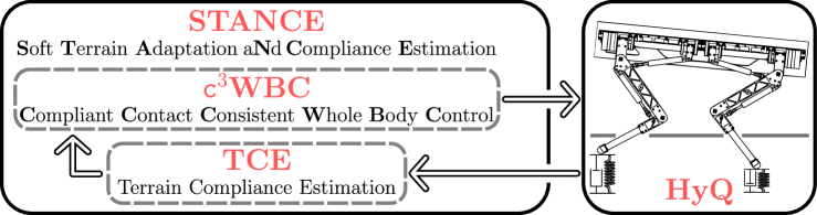
Figure 3.2: An overview of the STANCE algorithm.

3.1.3   Proposed Approach and Contribution

In this work, we propose an online soft terrain adaptation algorithm called: Soft Terrain Adaptation aNd Compliance Estimation (STANCE). As shown in Fig. 3.2, STANCE consists of

• A Compliant Contact Consistent Whole-Body Control (c³WBC) that is contact consistent to any type of terrain given the terrain compliance. This is done by extending the state-of-the-art WBC in [1], hereafter denoted as the Standard Whole-Body Control (sWBC). In particular, c³WBC incorporates a soft contact model into the WBC formulation.

• A Terrain Compliance Estimator (TCE) which is an online learning algorithm that provides the c³WBC with an estimate of the terrain compliance. It is based on the same contact model that is incorporated in the c³WBC.

The main contribution of STANCE is that it can adapt to any type of terrain (stiff or soft) online without pre-tuning. This is done by closing the loop of the c³WBC with the TCE. To our knowledge, this is the first implementation of such an approach in legged locomotion.

STANCE is meant to overcome the limitations of the aforementioned approaches in soft terrain adaptation for legged robots. Compared to previous works on WBC that tested their approach only during standing [29, 46], we test our STANCE approach during locomotion. Compared to other approaches [47, 48] that were tested on monopods in simulation, STANCE is implemented and tested in experiment on Hydraulically actuated Quadruped (HyQ). Compared to previous work on soft terrain adaptation [49], STANCE can adapt to soft terrain online and was tested on multiple terrains with different compliances and with transitions between them. Compared to [53], our TCE is computationally inexpensive, which allows STANCE to run real-time in experiments and simulations. Compared to the previous work done on compliance estimation, we implemented our TCE on a legged robot which is, to the best of our knowledge, the first experimental validation of this approach. Differently from [13], our TCE approach could be implemented in parallel with any gait or task. We also achieved a more accurate estimation of the terrain compliance compared to [13].

As additional contributions, we discussed the benefits (and the limitations) of exploiting the knowledge of the terrain in WBC based on the experience gained during extensive experimental trials. To our knowledge, STANCE is the first work to present legged locomotion experiments crossing multiple terrains of different compliances.

3.2  Robot model

Consider a legged robot with $n$ Degrees of Freedom (DoFs) and $c$ feet. The total dimension of the feet operational space $n_{{f}}$ can be separated into stance ($n_{\mathrm{st}}=3c_{\mathrm{st}}$) and swing feet ($n_{\mathrm{sw}}=3c_{\mathrm{sw}}$) where $c_{\mathrm{st}}$ and $c_{\mathrm{sw}}$ are the number of stance and swing legs respectively. Assuming that all external forces are exerted on the stance feet, the robot dynamics is written as

$$\underbrace{\begin{bmatrix}M_{\mathrm{com}}&0_{3\times 3}&0_{3\times n}\\ 0_{3\times 3}&M_{\theta}&M_{\theta j}\\ 0_{n\times 3}&M_{\theta j}^{T}&M_{j}\end{bmatrix}}_{M(q)}\underbrace{\begin{bmatrix}\ddot{x}_{\mathrm{com}}\\ \dot{\omega}_{b}\\ \ddot{q}_{j}\end{bmatrix}}_{\ddot{q}}+\underbrace{\begin{bmatrix}h_{\mathrm{com}}\\ h_{\theta}\\ h_{j}\end{bmatrix}}_{h(q,\dot{q})}$$

$$=\begin{bmatrix}0_{3\times 1}\\ 0_{3\times 1}\\ \tau_{j}\end{bmatrix}+\underbrace{\begin{bmatrix}J_{\mathrm{st,com}}^{T}\\ J_{\mathrm{st},\theta}^{T}\\ J_{\mathrm{st},j}^{T}\end{bmatrix}}_{J_{\mathrm{st}}(q)^{T}}F_{\mathrm{grf}}$$ (3.1)

where $q~{}\in~{}SE(3)~{}\times~{}\mathbb{R}^{n}$ denotes the generalized robot states consisting of the Center of Mass (CoM) position $x_{\mathrm{com}}$ $\in~{}\mathbb{R}^{3}$, the base orientation $R_{b}$ $\in~{}SO(3)$, and the joint positions $q_{j}$ $\in~{}\mathbb{R}^{n}$. The vector $\dot{q}~{}=~{}[\dot{x}_{\mathrm{com}}^{T}~{}\omega_{b}^{T}~{}\dot{q}_{j}^{T}]^{T}~{}\in~{}\mathbb{R}^{6+n}$ denotes the generalized velocities consisting of the velocity of the CoM $\dot{x}_{\mathrm{com}}$ $\in~{}\mathbb{R}^{3}$, the angular velocity of the base $\omega_{b}$ $\in~{}\mathbb{R}^{3}$, and the joint velocities $\dot{q}_{j}$ $\in~{}\mathbb{R}^{n}$. The vector $\ddot{q}~{}=~{}[\ddot{x}_{\mathrm{com}}^{T}~{}\dot{\omega}_{b}^{T}~{}\ddot{q}_{j}^{T}]^{T}~{}\in~{}\mathbb{R}^{6+n}$ denotes the corresponding generalized accelerations. All Cartesian vectors are expressed in the world frame $\Psi_{W}$ unless mentioned otherwise. $M~{}\in~{}\mathbb{R}^{(6+n)\times(6+n)}$ is the inertia matrix. $h\in\mathbb{R}^{6+n}$ is the force vector that accounts for Coriolis, centrifugal, and gravitational forces. $\tau_{j}\in\mathbb{R}^{n}$ are the actuated joint torques, $F_{\mathrm{grf}}\in\mathbb{R}^{n_{\mathrm{st}}}$ is the vector of GRFs (contact forces). The Jacobian matrix $J$ $\in\mathbb{R}^{n_{\mathrm{f}}\times(6+n)}$ is separated into swing Jacobian $J_{\mathrm{sw}}$ $\in\mathbb{R}^{n_{\mathrm{sw}}~{}\times~{}(6+n)}$ and stance Jacobian $J_{\mathrm{st}}~{}\in~{}\mathbb{R}^{n_{\mathrm{st}}~{}\times~{}(6+n)}$ which can be further expanded into $J_{\mathrm{st,com}}$ $\in\mathbb{R}^{n_{\mathrm{st}}\times 3}$, $J_{\mathrm{st,}\theta}$ $\in\mathbb{R}^{n_{\mathrm{st}}\times 3}$, and $J_{\mathrm{st},j}$ $\in\mathbb{R}^{n_{\mathrm{st}}\times n}$. The feet velocities $v~{}\in\mathbb{R}^{n_{\mathrm{f}}}$ are separated into stance $v_{\mathrm{st}}~{}\in~{}\mathbb{R}^{n_{\mathrm{st}}}$ and swing $v_{\mathrm{sw}}~{}\in~{}\mathbb{R}^{n_{\mathrm{sw}}}$ feet velocities. Similarly, the feet accelerations $\dot{v}~{}\in\mathbb{R}^{n_{\mathrm{f}}}$ are separated into stance $\dot{v}_{\mathrm{st}}~{}\in~{}\mathbb{R}^{n_{\mathrm{st}}}$ and swing $\dot{v}_{\mathrm{sw}}~{}\in~{}\mathbb{R}^{n_{\mathrm{sw}}}$ feet accelerations. The feet forces $F~{}=~{}[F_{\mathrm{st}}^{T}\ F_{\mathrm{sw}}^{T}]^{T}~{}\in~{}\mathbb{R}^{n_{\mathrm{f}}}$ are also separated into stance $F_{\mathrm{st}}~{}\in~{}\mathbb{R}^{n_{\mathrm{st}}}$ and swing $F_{\mathrm{sw}}~{}\in\mathbb{R}^{n_{\mathrm{sw}}}$ feet forces. We split the robot dynamics (3.1) into an unactuated floating base part (the first 6 rows) and an actuated part (the remaining $n$ rows) as

$$M_{u}(q)\ddot{q}+h_{u}(q,\dot{q}) = J_{\mathrm{st},u}(q)^{T}F_{\mathrm{grf}}$$ (3.2a)

$$M_{a}(q)\ddot{q}+h_{j}(q,\dot{q}) = \tau_{j}+J_{\mathrm{st},j}(q)^{T}F_{\mathrm{grf}}$$ (3.2b)

where $M_{u}$ $\in~{}\mathbb{R}^{6\times 6+n}$ and $M_{a}$ $\in~{}\mathbb{R}^{n\times 6+n}$ are sub matrices of $M$, $h_{u}=[h_{\mathrm{com}}^{T}~{}h_{\theta}^{T}]^{T}$ $\in~{}\mathbb{R}^{6}$ and $h_{j}$ $\in~{}\mathbb{R}^{n}$ are sub vectors of $h$, and $J_{\mathrm{st},u}=[J_{\mathrm{st,com}}^{T}~{}J_{\mathrm{st},\theta}^{T}]^{T}$. Finally, we define the gravito-inertial wrench as $W_{\mathrm{com}}~{}=~{}M_{u}(q)\ddot{q}+h_{u}(q,\dot{q})$ $\in\mathbb{R}^{6}$.

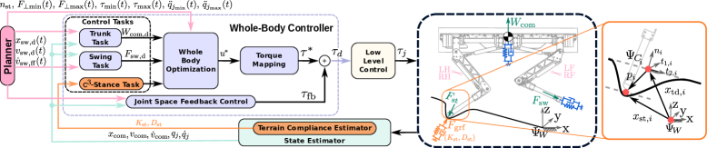
Figure 3.3: Overview of the WBC in our locomotion framework. The dashed black box presents the definition of the HyQ’s legs (LF, RF, LH and RH) and the generated wrenches. The solid orange box presents the terminologies used for the soft contact model. $\Psi_{\mathrm{W}}$ is the world frame and $\Psi_{\mathrm{C}_{i}}$ is the local contact frame for the leg $i$ fixed at the touch down position.

3.3  Standard Whole-Body Controller (sWBC)

This section summarizes the sWBC as detailed in [1]. Besides the WBC, our locomotion framework includes a locomotion planner, state estimator and a low-level torque controller as shown in Fig. 3.3. Given high-level user inputs, the planner generates the desired trajectories for the CoM, trunk orientation and swing legs, and provides them to the WBC. The state estimation provides the WBC with the estimated states of the robot.

The objective of the sWBC is to ensure the execution of the trajectories provided by the planner while keeping the robot balanced and reasoning about the robot’s dynamics, actuation limits and the contact constraints [1]. We denote the execution of the trajectories provided by the planner as control tasks. These control tasks alongside the aforementioned constraints define the WBC problem. The control problem is casted as a Whole-Body Optimization (WBOpt) problem via a Quadratic Program (QP) which solves for the optimal generalized accelerations and contact forces at each iteration of the control loop [27]. The optimal solution of the WBC is then mapped into joint torques that are sent to the low-level torque controller.

3.3.1   Control Tasks

We categorize the sWBC control tasks into: 1) a trunk task that tracks the desired trajectories of the CoM position and trunk orientation, and 2) a swing task that tracks the swing feet trajectories [1]. Similar to a PD+ controller [39], both tasks are achieved by a Cartesian-based impedance controller with a feed-forward term. The feedforward terms are added in order to improve the tracking performance of the tasks when following the trajectories from the planner [29, 34]. The tracking of the trunk task is obtained by the desired wrench at the CoM $W_{\mathrm{com,d}}\in\mathbb{R}^{6}$. This is generated by a Cartesian impedance at the CoM, a gravity compensation term, and a feed-forward term. Similarly, the tracking of the swing task can be obtained by the virtual force $F_{\mathrm{sw,d}}\in\mathbb{R}^{n_{\mathrm{sw}}}$. This is generated by a Cartesian impedance at the swing foot and a feed-forward term. As in [1], we can also write the swing task at the acceleration level by defining the desired swing feet velocities $\dot{v}_{\mathrm{sw,d}}$ $\in\mathbb{R}^{n_{\mathrm{sw}}}$ as

$$\dot{v}_{\mathrm{sw,d}}=\dot{v}_{\mathrm{sw,ff}}+\mathrm{K}_{\mathrm{sw}}\Delta x_{\mathrm{sw}}+\mathrm{D}_{\mathrm{sw}}\Delta v_{\mathrm{sw}}$$ (3.3)

where $\mathrm{K}_{\mathrm{sw}},\mathrm{D}_{\mathrm{sw}}\in\mathbb{R}^{n_{\mathrm{sw}}\times n_{\mathrm{sw}}}$ are positive definite PD gains, $\Delta x_{\mathrm{sw}}=x_{\mathrm{sw,d}}-x_{\mathrm{sw}}$ $\in\mathbb{R}^{n_{\mathrm{sw}}}$ and $\Delta v_{\mathrm{sw}}=v_{\mathrm{sw,d}}-v_{\mathrm{sw}}$ $\in\mathbb{R}^{n_{\mathrm{sw}}}$ are tracking errors of the swing foot position and velocity, respectively, and $\dot{v}_{\mathrm{sw,ff}}$ is a feed-forward term.

3.3.2   Whole-Body Optimization

To accomplish the sWBC objective (the control tasks in Section 3.3.1 and constraints), we formulate the WBOpt problem presented in Algorithm 1 and detailed in [1].

3.3.2.1   Decision Variables

As shown in Algorithm 1, we choose the generalized accelerations $\ddot{q}$ and the contact forces $F_{\mathrm{grf}}$ as the decision variables $u~{}=~{}[\ddot{q}^{T}~{}F_{\mathrm{grf}}^{T}]^{T}~{}\in~{}\mathbb{R}^{6+n+n_{\mathrm{st}}}$. Later in this subsection, we will augment the vector of decision variables with a slack term $\eta\in\mathbb{R}^{n_{\mathrm{sw}}}$.

3.3.2.2   Cost

The cost function (3.5) consists of two terms. The first term ensures the tracking of the trunk task by minimizing the two-norm of the tracking error between the actual $W_{\mathrm{com}}$ and desired $W_{\mathrm{com,d}}$ CoM wrenches. The second term in (3.5) regularizes the solution and penalizes the slack variable.

3.3.2.3   Physical Consistency

The equality constraint (3.6) enforces the physical consistency between $F_{\mathrm{grf}}$ and $\ddot{q}$ by ensuring that the contact wrenches due to $F_{\mathrm{grf}}$ will sum up to $W_{\mathrm{com}}$. This is done by imposing the unactuated dynamics (3.2a) as an equality constraint.

3.3.2.4   Stance Task

To remain contact consistent, we incorporate the stance task that enforces the stance legs to remain in contact with the terrain. Since the sWBC is assuming a rigid terrain, the stance feet are forced to remain stationary in the world frame, i.e., $v_{\mathrm{st}}=\dot{v}_{\mathrm{st}}=0$ (see [1]). As a result, we incorporate the rigid contact model in the sWBC formulation as an equality constraint at the acceleration level (3.7) in order to have a direct dependency on the decision variables. In detail, since $v_{\mathrm{st}}=J_{\mathrm{st}}\dot{q}=0$, differentiating once with respect to time yields $\dot{v}_{\mathrm{st}}=J_{\mathrm{st}}\ddot{q}+\dot{J}_{\mathrm{st}}\dot{q}=0$.

3.3.2.5   Friction and Normal Contact Force

The inequality constraint (3.11) enforces the friction constraints by ensuring that the contact forces lie inside the friction cones. This is done by limiting the tangential component of the GRFs $F_{\mathrm{grf,\parallel}}$. The inequality constraint (3.12) enforces constraints on the normal component of the GRFs $F_{\mathrm{grf,\perp}}$. This includes the unilaterality constraints which encodes that the legs can only push on the ground by setting an “almost-zero” lower bound $F_{\mathrm{\min}}$ to $F_{\mathrm{grf,\perp}}$. They also allow a smooth loading/unloading of the legs, and set a varying upper bound $F_{\mathrm{\max}}$ to $F_{\mathrm{grf,\perp}}$. For the detailed implementation of the inequality constraints (3.11) and (3.12), refer to [34].

3.3.2.6   Swing Task

We implement the tracking of the swing task (in Section 3.3.1) at the acceleration level (3.3) rather than the force level since we can express the swing feet velocities $\dot{v}_{\mathrm{sw}}$ as a function of $\ddot{q}$ which is a decision variable, i.e., $\dot{v}_{\mathrm{sw}}(q)=J_{\mathrm{sw}}\ddot{q}+\dot{J}_{\mathrm{sw}}\dot{q}$. This task could be encoded as an equality constraint $\dot{v}_{\mathrm{sw}}=\dot{v}_{\mathrm{sw,d}}$. Yet, it is important to relax this hard constraint when the joint kinematic limits are reached (see [1]). Hence, the swing task is encoded in (3.13) by an inequality constraint that bounds the solution around the original hard constraint and a slack term $\eta$ that is penalized for its non-zero values in the cost function (3.5) and is constrained to remain non-negative in (3.13).

3.3.2.7   Torque and Joint Limits

The torque and joint limits are enforced in the inequality constraints (3.14) and (3.15), respectively.

3.3.2.8   Torque Mapping

The WBOpt (3.5)-(3.7), (3.11)-(3.15) generates optimal joint accelerations $\ddot{q}_{j}^{*}$ and contact forces $F_{\mathrm{grf}}^{*}$, that are mapped into optimal joint torques $\tau^{*}$ and sent to the low-level controller using the actuated dynamics (3.2b) as

$$\tau^{*}=M_{a}\ddot{q}^{*}+h_{j}-J_{\mathrm{st},j}^{T}F_{\mathrm{grf}}^{*}$$ (3.4)

Algorithm 1 Whole-Body Optimization: sWBC Vs. c³WBC

(Trunk Task) (Decision Variables) (Physical Consistency) (Stance Task) (c³-Stance Task) (Friction) (Normal Contact Force) (Swing Task) (Torque Limits) (Joint Limits) $$\underset{u}{\text{min~{}}}\|W_{\mathrm{com}}-W_{\mathrm{com,d}}\|^{2}_{Q}+{\color[rgb]{0,0.5,1}\bm{\|u\|^{2}_{R}}} u=[\ddot{q}^{T}\ F_{\mathrm{grf}}^{T}\ \eta^{T}\ {\color[rgb]{0,0.5,1}\bm{\epsilon^{T}}}]^{T} M_{u}\ddot{q}+h_{u}=J^{T}_{\mathrm{st},u}F_{\mathrm{grf}} {\color[rgb]{0,0.5,1}\bm{F_{\mathrm{grf}}=K_{\mathrm{st}}\epsilon+D_{\mathrm{st}}\dot{\epsilon}}} {\color[rgb]{0,0.5,1}\bm{\dot{v}_{\mathrm{st}}=J_{\mathrm{st}}\ddot{q}+\dot{J}_{\mathrm{st}}\dot{q}=-\ddot{\epsilon}}} {\color[rgb]{0,0.5,1}\bm{\epsilon\geq 0}} |F_{\mathrm{grf,\parallel}}|\leq\mu|F_{\mathrm{grf,\perp}}| F_{\mathrm{\min}}\leq F_{\mathrm{grf,\perp}}\leq F_{\mathrm{\max}} -\eta\leq\dot{v}_{\mathrm{sw}}-\dot{v}_{{\mathrm{sw,d}}}\leq\eta,~{}\eta\geq 0 \tau_{\min}\leq\tau_{j}\leq\tau_{\max} \ddot{q}_{j_{\min}}\leq\ddot{q}_{j}\leq\ddot{q}_{j_{\max}}$$ (3.5) s.t.: (3.6) (3.7) (3.8) (3.9) (3.10) (3.11) (3.12) (3.13) (3.14) (3.15)

3.3.3   Feedback Control

The computation of the optimal torques $\tau^{*}$ relies on the inverse dynamics in (3.4) which might be prone to model inaccuracies [59]. In order to tackle this issue, the desired torques $\tau_{d}$ sent to the lower level control could combine the optimal torques $\tau^{*}$ in (3.4) with a feedback controller $\tau_{\mathrm{fb}}$ as shown in Fig. 3.3. The feedback controller improves the tracking performance if the dynamic model of the robot becomes less accurate [59]. The feedback controller is a proportional-derivative (PD) joint space impedance controller [34].

Remark 3.1

Throughout this work and similar to [1] and [27], we found it sufficient to use only the inverse-dynamics term (the optimal torques $\tau^{*}$) and not the joint feedback part. This is due to the fact that we can identify the parameters of our dynamic model with sufficient accuracy as detailed in [60]. That said, we carried out the simulation and experiment without any need of the feedback loop.

3.4  C³ Whole-Body Controller

Over soft terrain, the feet positions are non-stationary and are allowed to deform the terrain. Thus, the rigid contact assumption of the stance task (3.7) in the sWBC does not hold anymore and should be dropped. To be c³, the interaction between the stance feet and the soft terrain must be governed not just by the robot dynamics but also by the soft contact dynamics. That said, the c³WBC extends the sWBC by: 1) modeling the soft contact dynamics and incorporating it as a stance task similar to the control tasks in Section 3.3.1, and 2) encoding the stance task in the WBOpt as a function of the decision variables. The differences between the sWBC and the c³WBC are highlighted in boldface in Algorithm 1.

Remark 3.2

The term contact consistent is a well-established term in the literature that was initially introduced in [61]. It implies formulating the control structure to account for the contact with the environment. The term c³ is an extension of the term contact consistent. Hence, c³ implies formulating the control structure to account for the compliant contact with the environment.

3.4.1   c³-Stance Task

We model the soft contact dynamics with a simple explicit model (the KV model). This consists of 3D linear springs and dampers normal and tangential to the contact point [51]. The normal direction of this impedance emulates the normal terrain deformation while the tangential ones emulate the shear deformation. Although several models that accurately emulate contact dynamics are available [62, 63, 54], we implemented the KV model for several reasons. First, since the model is linear in the parameters, it fits our QP formulation. Second, estimating the parameters of the KV model is computationally efficient. As a result, using this model, we can run a learning algorithm online which would be challenging if a model similar to [53] is used. For a legged robot with point-like feet, for each stance leg $i$, we formulate the contact model in the world frame as

$$F_{\mathrm{grf,i}}=k_{\mathrm{st},i}p_{i}+d_{\mathrm{st},i}\dot{p}_{i}$$ (3.16)

where $k_{\mathrm{st},i}\in\mathbb{R}^{3\times 3}$, $d_{\mathrm{st},i}\in\mathbb{R}^{3\times 3}$, $F_{\mathrm{grf,i}}\in\mathbb{R}^{3}$, $p_{i}\in\mathbb{R}^{3}$, and $\dot{p}_{i}\in\mathbb{R}^{3}$ are the terrain stiffness, the terrain damping, the GRFs, the penetration and the penetration rate of the $i$-th stance leg, all expressed in the world frame, respectively (see Fig. 3.3). We define $p_{i}$ and $\dot{p}_{i}$ as

$$p_{i}=x_{\mathrm{td},i}-x_{\mathrm{st},i}\text{,}\hskip 50.00008pt\dot{p}_{i}=0-v_{\mathrm{st},i}$$ (3.17)

where $x_{\mathrm{td},i}\in\mathbb{R}^{3}$ denotes the position of the contact point of foot $i$ at the touchdown in the world frame. By appending all of the stance feet, the contact model can be re-written in a compact form as

$$F_{\mathrm{grf}}=K_{\mathrm{st}}p+D_{\mathrm{st}}\dot{p}=K_{\mathrm{st}}(x_{\mathrm{td}}-x_{\mathrm{st}})-D_{\mathrm{st}}v_{st}$$ (3.18)

where $K_{\mathrm{st}}$ $\in R^{n_{\mathrm{st}}\times n_{\mathrm{st}}}$ and $D_{\mathrm{st}}$ $\in R^{n_{\mathrm{st}}\times n_{\mathrm{st}}}$ are the block-diagonal stiffness and damping matrices of the terrain of all the stance feet, respectively, and $x_{\mathrm{td}}$ $\in\mathbb{R}^{n_{st}}$ are the touchdown positions of all the stance feet.

Similar to Section 3.3.1, we deal with the contact model (3.18) as another WBC task (alongside the trunk and swing (3.3) tasks). We can think of (3.18) as a desired stance task that keeps the WBC c³. This stance task is achieved by a Cartesian impedance at the stance foot which is represented by the impedance of the terrain ($K_{\mathrm{st}}$ and $D_{\mathrm{st}}$). This similarity makes us encode the contact model in the WBOpt as a stance constraint similar to what we did for the swing task in Section 3.3.2. Hereafter, we refer to this stance task as the c³-stance task (see Fig. 3.3).

3.4.2   Whole-Body Optimization Revisited

The c³-stance task is included in the WBOpt by writing the soft contact model (3.18) as a function of the decision variables. Ideally, we can directly reformulate (3.18) as a function of $F_{\mathrm{grf}}$ and $\dot{v}_{\mathrm{st}}$. Indeed, $\dot{v}_{\mathrm{st}}$ can be expressed as a function of the joint accelerations $\ddot{q}$ which is a decision variable (as explained in [1]). By numerically integrating $\dot{v}_{\mathrm{st}}$ (once to obtain $v_{\mathrm{st}}$ and twice to obtain $x_{\mathrm{st}}$), we can associate $F_{\mathrm{grf}}$ with $\dot{v}_{\mathrm{st}}$. This approach requires the knowledge of $x_{\mathrm{td}}$ to compute $p$ which might be prone to estimation errors and it requires a reset of the integrator at every touchdown.

We choose a more convenient approach which is to add the desired foot penetration $\epsilon$ as an extra decision variable in the WBOpt formulation. The difference between $p$ and $\epsilon$ is that $p$ is the actual penetration due to the interaction with the soft contact while $\epsilon$ is the desired penetration in the world frame generated from the optimization problem. Both variables imply the same physical phenomenon (the soft contact deformation). That said, we can rewrite $F_{\mathrm{grf}}$ in (3.18) as a function of $\epsilon$ and $\dot{\epsilon}$ (by numerically differentiating $\epsilon$) without the previous knowledge of $x_{\mathrm{td}}$, which is advantageous.

To do so, $\epsilon$ is appended to the vector of decision variables $u$ and regularized in (3.5). Then, we incorporate (3.18) directly as a function of $F_{\mathrm{grf}}$ and $\epsilon$ as in the equality constraint (3.8). We numerically differentiate $\epsilon$ to obtain $\dot{\epsilon}_{k}=\frac{\epsilon_{k}-\epsilon_{k-1}}{\Delta t}$. To maintain physical consistency, we need to enforce an additional constraint between the desired penetration $\epsilon$ and the contact acceleration ($\ddot{\epsilon}=-\dot{v}_{\mathrm{st}}$). This is encoded as an equality constraint as shown in (3.9). To do so, we numerically differentiate $\epsilon$ twice to obtain $\ddot{\epsilon}_{k}=\frac{\epsilon_{k}-2\epsilon_{k-1}+\epsilon_{k-2}}{\Delta t^{2}}$. We also ensure the consistency of the physical contact model throughout the optimization problem by ensuring that the penetration is always positive in (3.10).

We also consider the loading and unloading phase, explained in [1] and [34], to be terrain-aware. We tune the loading and unloading phase period $T_{l/u}$ for each leg to follow the settling time of a second order system response that is a function of the terrain compliance and the robot’s mass [64]. Hence, $T_{l/u}$ is

$$T_{l/u}=4.6/\sqrt{\frac{k_{\mathrm{st,i}}}{m_{e}}}$$ (3.19)

where $m_{e}$ is the equivalent mass felt at the robot’s feet (i.e., the weight of the robot $m_{R}$ spread across its stance feet $m_{e}~{}=~{}m_{R}/n_{\mathrm{st}}$) and the constant in the numerator represents a $1\%$ steady-state error.

Finally, the WBOpt (3.5), (3.6), (3.8)-(3.15) generates optimal joint accelerations $\ddot{q}_{j}^{*}$ and contact forces $F_{\mathrm{grf}}^{*}$, that are mapped into optimal joint torques $\tau^{*}$ and sent to the low-level controller using the actuated part of the robot’s dynamics as shown in (3.4). Note that similar to the sWBC, we found it sufficient to use only the inverse-dynamics term (the optimal torques $\tau^{*}$) and not the joint feedback part.

As explained above, adding $\epsilon$ as a decision variable involved adding two constraints in the optimization which increases the problem size and the computation time. Yet, we are still able to run the c³WBC in real-time. The advantage of our approach is that the knowledge of the touchdown position $x_{\mathrm{td}}$ is not required. We only need the previous two time instances of the penetration $\epsilon_{k-1}$ and $\epsilon_{k-2}$ that we already computed in the previous control loops.

3.5  Terrain Compliance Estimation

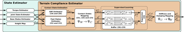
Figure 3.4: Overview of the TCE’s architecture inside the state estimator.

The purpose of the TCE is to estimate online the terrain parameters (namely $K_{\mathrm{st}}$ and $D_{\mathrm{st}}$) based on the states of the robot. It is a stand-alone algorithm that is decoupled from the c³WBC. The TCE uses the contact model (3.18). Based on that, the current measurement of the contact states (contact status $\alpha$, GRFs $F_{\mathrm{grf}}$, the penetration $p$, and the penetration rate $\dot{p}$) of each leg $i$ at every time step are required. Given the contact states, we use supervised learning to learn the terrain parameters. As shown in Fig. 3.4, the TCE consists of two main modules: contact state estimation (Section 3.5.1) and supervised learning (Section 3.5.2). The contact state estimation module estimates the contact states and provides it to the supervised learning module that collects these data and computes the estimates of the terrain parameters.

3.5.1   Contact State Estimation

The contact states are estimated solely from the current states of the robot by the state estimator. The GRFs are estimated from the torques and the joint states, and the penetration and its rate are estimated from the floating base (trunk) states and the joint states.

3.5.1.1   GRFs Estimation

To estimate the GRF, we use actuated part of the dynamics in (3.2b) as

$$F_{\mathrm{grf},i}=\alpha_{i}J_{j,i}^{-T}(M_{a,i}\ddot{q}_{i}+h_{j,i}-\tau_{j,i})$$ (3.20)

where $F_{\mathrm{grf},i}$, $J_{j,i}$, $M_{a,i}$, $\ddot{q}_{i}$, $h_{j,i}$, and $\tau_{j,i}$ correspond to $F_{\mathrm{grf}}$, $J_{\mathrm{st},j}$, $M_{a}$, $\ddot{q}$, $h_{j}$, and $\tau_{j}$ for the $i$-th leg, respectively. Additionally, $\alpha_{i}$ is the contact status variable that detects if there is a contact in the $i$-th leg or not. The contact is detected when the GRFs exceed a certain threshold $F_{\min}$. Hence, $\alpha_{i}$ computed along the normal direction of the $i$-th leg $n_{i}$ as:

$$\alpha_{i}=\begin{cases}1,&\text{if $n_{i}^{T}(J_{j,i}^{-T}(M_{a,i}\ddot{q}_{i}+h_{j,i}-\tau_{j,i})\geq F_{\min}$}\\ 0,&\text{otherwise}\end{cases}$$ (3.21)

3.5.1.2   Penetration Estimation

As shown in (3.17), we estimate the penetration and its rate using the stance feet positions $x_{\mathrm{st},i}$ and velocities $v_{\mathrm{st},i}$, and the touchdown position $x_{\mathrm{td},i}$ all in the world frame. To estimate the feet states in the world frame, we use the forward kinematics and the base state in the world frame. Thus, the penetration and its rate are written as

$$p_{i} = x_{\mathrm{td},i}-x_{\mathrm{st},i}=x_{\mathrm{td},i}-x_{b}-R_{B}^{W}x_{\mathrm{st},i}^{B}$$ (3.22)

$$\dot{p}_{i} = -v_{\mathrm{st},i}=-v_{b}-R_{B}^{W}v_{\mathrm{st},i}^{B}-(\omega_{b}\times R_{B}^{W})x_{\mathrm{st},i}^{B}$$ (3.23)

where $x_{b}$ $\in\mathbb{R}^{3}$ and $v_{b}$ $\in\mathbb{R}^{3}$ are the base position and velocity in the world frame, respectively. The terms $x_{\mathrm{st},i}^{B}$ and $v_{\mathrm{st},i}^{B}$ are the stance feet position and velocity of the $i$-th leg in the base frame, respectively. The terms $R_{B}^{W}$ $\in SO(3)$ and $\omega_{b}$ are the rotation matrix mapping vectors from the base frame to the world frame and the base angular velocity, respectively. The touch down positions are obtained using a height map.

3.5.1.3   Contact States Mapping

Since, the KV model consists of 3D linear springs and dampers, normal and tangential to the contact point, this makes the stiffness and damping matrices diagonal with respect to the contact frame. However, if expressed in the world frame, the stiffness and damping matrices become dense. Thus, if we formulate the KV model in the contact frame rather than the world frame, we estimate less number of elements per matrix per leg: three elements instead of nine. Henceforth, the KV model in the TCE should be formulated with respect to the contact frame rather than the world frame to reduce the computational complexity. To do so, the GRFs (3.20), the penetration (3.22) and its rate (3.23) of the $i$-th leg are transformed from the world frame $\Psi_{W}$ to the contact frame $\Psi_{C_{i}}$ as (see Fig. 3.3)

$$F_{\mathrm{grf},i}^{C} = R_{W}^{C_{i}}F_{\mathrm{grf,i}}$$ (3.24)

$$p_{i}^{C} = R_{W}^{C_{i}}p_{i}$$ (3.25)

$$\dot{p}_{i}^{C} = R_{W}^{C_{i}}\dot{p}_{i}$$ (3.26)

where the superscript $\bullet^{C}$ refers to the contact frame and $R_{W}^{C_{i}}$ is the rotation matrix mapping from the world $\Psi_{W}$ to the contact $\Psi_{C_{i}}$ frames for the $i$-th leg. Note that the transformation (3.26) is linear since the contact frame is fixed with respect to the world frame at the touch down position (i.e., $\dot{R}_{W}^{C_{i}}=0$).

3.5.2   Supervised Learning

Considering the contact model in the contact frame and using the estimated contact states (3.24)-(3.26), we learn the terrain parameters online via supervised learning. In particular, we use weighted linear least squared regression. The algorithm is treated as a batch algorithm with $m$-examples such that, at every time instant $k$, we gather samples from the previous $m$ time instances and compute the terrain parameters [65].

For the $k$-th time instant, of the $i$-th leg in the $d\text{-th}$ direction ($d\in\{n_{i},t_{1,i},t_{2,i}\}$, see Fig. 3.3), the terms $F_{\mathrm{grf},i}^{C,d}(k)$, $p_{i}^{C,d}(k)$, and $\dot{p}_{i}^{C,d}(k)$ are estimated as shown in Section 3.5.1 where $\bullet_{i}^{d}(k)$ refers to the $k$-th time instance of the $i$-th leg in the $d$-th direction. That said, we construct the following objects (buffers) with size $m$

$$\mathcal{F}_{i}^{d} = \begin{bmatrix}F_{\mathrm{grf},i}^{C,d}(k)&\cdots&F_{\mathrm{grf},i}^{C,d}(k-m)\end{bmatrix}^{T}$$ (3.27)

$$\mathrm{P}_{i}^{d} = \begin{bmatrix}p_{i}^{C,d}(k)&\cdots&p_{i}^{C,d}(k-m)\end{bmatrix}^{T}$$ (3.28)

$$\dot{\mathrm{P}}_{i}^{d} = \begin{bmatrix}\dot{p}_{i}^{C,d}(k)&\cdots&\dot{p}_{i}^{C,d}(k-m)\end{bmatrix}^{T}$$ (3.29)

$$\mathcal{P}_{i}^{d} = \begin{bmatrix}\mathrm{P}_{i}^{d}&\dot{\mathrm{P}}_{i}^{d}\end{bmatrix}$$ (3.30)

where $\mathcal{F}_{i}^{d}\in\mathbb{R}^{m}$ is the GRFs buffer and $\mathcal{P}_{i}^{d}\in\mathbb{R}^{m\times 2}$ is the penetration, and penetration rate buffer. Given $\mathcal{F}_{i}^{d}$ and $\mathcal{P}_{i}^{d}$ as inputs and outputs of the learning algorithm respectively, we estimate the terrain impedance parameters as $I_{i}^{d}=\begin{bmatrix}k_{\mathrm{st},i}^{C,d}~{}d_{\mathrm{st},i}^{C,d}\end{bmatrix}^{T}\in\mathbb{R}^{2}$ using the analytical solution

$$I_{i}^{d}=(\mathcal{P}_{i}^{dT}W\mathcal{P}_{i}^{d})^{-1}\mathcal{P}_{i}^{dT}W\mathcal{F}_{i}^{d}$$ (3.31)

where $k_{\mathrm{st},i}^{C,d}\in\mathbb{R}$ and $d_{\mathrm{st},i}^{C,d}\in\mathbb{R}$ are the terrain stiffness and damping parameters expressed in the contact frame. The matrix $W\in\mathbb{R}^{m\times m}$ is a weighting matrix used to penalize the error on most recent sample compared to the less recent ones and thus, giving more importance to the most recent samples.

All of the legs in the learning algorithm are decoupled. We found it advantageous to treat each leg separately because the robot can be standing on a different terrain at each foot.

3.5.3   Implementation Details

Algorithm 2 sketches the entire TCE process. To initialize the buffers, we acquire samples when the robot is at full stance and return the first estimate of $I_{i}^{d}$ once the buffers are full. After initialization, we acquire samples and update the buffers only when the leg is at stance.

The buffers are continuously updated in a sliding window fashion. When a leg finishes the swing phase and is at a new touch down, it continues to use the previous samples from the previous stance phase. This is advantageous since it gives a smooth transition between terrains, but it adds a delay.

Remark 3.3

Since the c³WBC formulation is based in the world frame, it is essential to map the estimated stiffness and damping matrices back to the world frame before providing them to the c³WBC (see Fig. 3.4).

Remark 3.4

The TCE can be used with any arbitrary terrain geometry given the terrain normal and thus $R_{W}^{C_{i}}$. The terrain normal $n_{i}$ at the contact point $i$ can be provided by a height map that is generated via an RGBD sensor.

Algorithm 2 Terrain Compliance Estimation

1:initialize the buffers ($\mathcal{F}_{i}^{d}$ and $\mathcal{P}_{i}^{d}$) and $I_{i}^{d}$

2:for each iteration $k$ do

3:     for each leg $i$ do

4:         if leg is in contact ($\alpha_{i}==1$) then(3.21)

5:              for each direction $d$ do

6:                  estimate $F_{\mathrm{grf,i}}^{d}(k)$ (3.20)

7:                  estimate $p_{i}^{d}(k)$ (3.22)

8:                  estimate $\dot{p}_{i}^{d}(k)$ (3.23)

9:                  transform $F_{\mathrm{grf,i}}^{d}(k)$ into $F_{\mathrm{grf},i}^{C,d}(k)$ (3.24)

10:                  transform $p_{i}^{d}(k)$ into $p_{i}^{C,d}(k)$ (3.25)

11:                  transform $\dot{p}_{i}^{d}(k)$ into $\dot{p}_{i}^{C,d}(k)$ (3.26)

12:                  update buffers $\mathcal{F}_{i}^{d}$ and $\mathcal{P}_{i}^{d}$ (3.27)-(3.30)

13:                  solve for $I_{i}^{d}$ (3.31)

14:              end for

15:              map the estimated parameters to $\Psi_{W}$

16:         end if

17:     end for

18:end for

3.6  Experimental Setup

3.6.1   State Estimation

We implemented our approach on HyQ [66] which is equipped with a variety of sensors. Each leg contains two load-cells, one torque sensor, and three high-resolution optical encoders. A tactical-grade Inertial Measurement Unit (IMU) (KVH 1775) is mounted on its trunk. Of particular importance to this experiment is the Vicon Motion Capture System (MCS). It is a multi-camera infrared system capable of measuring the pose of an object with high accuracy. During experiments, an accurate and non-drifting estimate of the position of the feet in the world frame is required to calculate the real penetration for the TCE. Typically, HyQ works independently of external sensors (e.g., MCS or GPS), however, soft terrain presents problems for state estimators [29]. This was re-affirmed in experiment.

The current state estimator [67] relies upon fusion of IMU and leg odometry data at a high frequency and uses lower frequency feedback from cameras or lidars to correct the drift. The leg odometry makes the assumption that the ground is rigid. On soft terrain, the estimator has difficulties in determining when a foot is in contact with the ground (i.e., is the foot in the air, or compressing the surface?). These errors cause the leg odometry signal to drift jeopardizing the estimation. Although, incorporating vision information could be a possibility to correct for the drift in the estimation, improving state estimation on soft terrain is an ongoing area of research and is out of the scope of this paper.

Despite the drifting problem, we used the current state estimator [67] in our WBC because the planner in Fig. 3.3 has a re-planning feature that makes our WBC robust against a drifting state estimator [41]. However, the TCE still requires an accurate and non drifting estimate of the feet position in the world frame. Therefore, to validate the TCE, we used an external MCS that completely eliminates the drift problem. The MCS measures the pose of a special marker array placed on the head of the robot. Then the position of the feet in the world frame was calculated online by using the MCS measurement and the forward kinematics of the robot.

3.6.2   Terrain Compliance Estimator (TCE) Settings

In this work we used a sliding window of $m=250$ samples (or 1 s for a control loop running at 250 Hz). Despite the general formulation, in this paper we estimate the terrain parameters only for the direction normal to the terrain, and assume that the tangential directions are the same. We carried out the simulation and experiment on a horizontal plane. Thus, the rotation matrix $R_{W}^{C_{i}}$ is identity. Furthermore, we did not estimate the damping parameter due to the inherent noise in the feet velocity signals that would jeopardize the estimation. The damping term $D_{\mathrm{st}}v_{st}$ in (3.18) is less dominant in computing the GRFs compared to the stiffness term. This is because the feet velocities in the world frame $v_{st}$ are usually orders of magnitude smaller than the penetration during stance, and the damping parameter $D_{\mathrm{st}}$ is usually orders of magnitude smaller than the stiffness parameter as shown in [63].

3.6.3   Tuning of the Low Level Control

During experiments, we found that the low level torque loop creates system instabilities when interacting with soft environments.

In particular, when we used the same set of (high) torque gains in the low level control loop tuned for rigid terrain, we noticed joint instabilities when walking over soft terrain. This is because interacting with soft terrain reduces the stability margins of the system. Thus, keeping a high bandwidth in the inner torque loop given the reduced stability margin will cause system instability. In our previous work [68], we experimentally validated that increasing the torque gain of the inner loop can indeed cause system instabilities. In fact, this is a well know issue in haptics [69]. As a result, reducing the bandwidth by decreasing the torque gains in the inner torque loop was necessary to address these instabilities.

Our control design is a nested architecture consisting of the WBC and the low level torque control in which, both control loops contribute to the system stability [68, 70]. Over soft terrain, the dynamics of the environment also plays a role and must be considered in analyzing the stability of the system. That said, there is a nontrivial relationship between soft terrain and the stability of a nested control loop architecture, and a formal and thorough analysis is an ongoing work.

3.7  Results

In this section, we evaluate the proposed approach on HyQ in simulation and experiment. We compare three approaches: the sWBC which is the baseline, the c³WBC which is our proposed WBC without the TCE, and STANCE which incorporates both the c³WBC and TCE. We show the extent of improvement given by the c³WBC controller with respect to the sWBC as well as the importance of the TCE during locomotion over multiple terrains with different compliances. We set the same parameters and gains throughout the entire simulations and experiments, unless mentioned otherwise. The results are shown in the accompanying video.

3.7.1   Simulations

To render soft terrain in simulation, we used the Open Dynamics Engine (ODE) physics engine [71]. We used ODE because it is easily integrable with our framework, and it is numerically fast and stable for stiff and soft contacts [72]. Moreover, ODE can render soft contacts that emulates physical parameters (using the SI units N/m and Ns/m for springs and dampers, respectively) unlike other engines that uses non-physical ones [73]. ODE’s implicit solver uses linear springs and dampers for their soft constraints which fits perfectly with our contact model (3.18). In this way, we have a controlled simulation environment where we can emulate any terrain compliance by manipulating its stiffness $K_{t}$ and damping $D_{t}$ parameters similar to our contact model. Throughout the simulation, we use four types of terrains with the following parameters: soft $T_{1}$ ($K_{t}=3500$ N/m), moderate $T_{2}$ ($K_{t}=8000$ N/m), stiff $T_{3}$ ($K_{t}=10000$ N/m), and rigid $T_{4}$ ($K_{t}=2\times 10^{6}$ N/m) all with the same damping ($D_{t}=400$ Ns/m).

3.7.1.1   Locomotion over Multiple Terrains

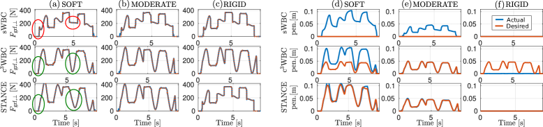
Figure 3.5: Simulation. Comparison of sWBC, c³WBC, and STANCE over three type of terrains: soft $T_{1}$ ($K_{t}=3500$ N/m), moderate $T_{2}$ ($K_{t}=8000$ N/m), and rigid $T_{4}$ ($K_{t}=2\times 10^{6}$ N/m) all with the same damping ($D_{t}=400$ Ns/m). (a)-(c): The actual and desired contact forces in the normal direction of the LF leg for one gait cycle. (d)-(f): The actual $p$ and desired $\epsilon$ penetration in the normal direction of the LF leg for one gait cycle. The red and green ellipses highlight the performance of the three approaches in adapting to soft terrain.

Table 3.1: Mean Absolute Tracking Error (MAE) [N] of the GRFs in Simulation using sWBC, c³WBC and STANCE over Multiple Terrains.

Terrain	sWBC	c3WBC	STANCE
Soft	7.7261	7.4419	6.3547
Moderate	8.0594	7.4585	7.9889
Rigid	4.889	6.6523	5.128

We evaluate the three approaches with the robot walking at $0.05$ m/s over the terrains: $T_{1}$ (soft), $T_{2}$ (moderate), and $T_{4}$ (rigid). We provided the c³WBC with the terrain parameters of the moderate terrain $T_{2}$ for all the three simulations. We do that in order to test the performance of c³WBC if given the real terrain parameters (in case of $T_{2}$) or inaccurate parameters (in case of $T_{1}$ and $T_{4}$). In this simulation, we compare the actual values of $F_{\mathrm{grf,\perp}}$ against the optimal values $F_{\mathrm{grf,\perp}}^{*}$(solution of the WBOpt) as well as the actual penetration $p$ against the desired penetration $\epsilon$ of the Left-Front (LF) leg. We have omitted the other three feet for space as all four legs have the same performance. The results are shown in Fig. 3.5. The Mean Absolute Tracking Error (MAE) of the GRFs in these simulations are presented in Table 3.1. The MAE of the GRFs is defined as: $\text{MAE}=\frac{1}{T}\int_{0}^{T}|F_{\mathrm{grf}}-F_{\mathrm{grf}}^{*}|dt$.

Fig. 3.5a captures the effect of the three approaches on the GRFs over soft terrain. We can see that a WBC based on a rigid contact assumption (sWBC) assumes that it can achieve an infinite bandwidth from the terrain and thus supplying an instantaneous change in the GRFs as highlighted by the red ellipses in Fig. 3.5a. On the other hand, STANCE and c³WBC were both capable of attenuating this effect as highlighted by the green ellipses. For the reasons explained earlier in this paper and in [49], instantaneous changes in the GRFs are undesirable over soft terrain. This resulted in an improvement in the tracking of the GRFs in STANCE and c³WBC compared to sWBC as shown in Table 3.1. Moreover, by comparing c³WBC and STANCE over soft terrain $T_{1}$, we can see that the shape of the GRFs did not differ. However, the tracking of the GRFs in STANCE is better than the c³WBC. This shows that suppling the c³WBC with the incorrect values of the terrain parameters deteriorates the GRFs tracking performance. Fig. 3.5b shows the GRFs on a moderate terrain. Since the c³WBC is provided with the exact terrain parameters of $T_{2}$, we can perceive the c³WBC as STANCE with a perfect TCE on moderate terrain. As a result, Table 3.1 shows that in this set of simulations, c³WBC outperformed STANCE in the GRFs tracking. This shows that a more accurate TCE can result in a better GRFs tracking. Additionally, Fig. 3.5c shows the GRFs on rigid terrain. We can see that the sWBC resulted in a typical (desired) shape of the GRFs for a crawl motion in rigid terrain [41]. STANCE showed a shape of the GRFs similar to the sWBC which is expected since the TCE provided STANCE with parameters similar to the rigid terrain. However, for c³WBC, the GRFs shape did not change compared to the other three terrains. As shown in Table 3.1, the best tracking to the GRFs was by the sWBC, which was expected since the sWBC was designed for rigid terrain. However, sWBC was only slightly better than STANCE due to small estimation errors from the TCE.

Fig. 3.5a-c show the superiority of STANCE compared to sWBC and c³WBC. STANCE adapted to the three terrains by estimating their parameters and supplying them to the WBC. This resulted in changing the shape of the GRFs accordingly that improved the tracking of the GRFs. Unlike STANCE, the sWBC and the c³WBC both are contact consistent for only one type of terrain which resulted in a deterioration of the GRFs tracking over the other types of terrains. The advantages of STANCE compared to sWBC and c³WBC are also shown in Fig. 3.5d-f. Since the sWBC is always assuming a rigid contact, the penetration $\epsilon$ was always zero throughout the three terrains. Similarly, since the c³WBC alone is aware only of one type of terrain, it is always assuming the same contact model, in which the desired penetration $\epsilon$ was similar throughout the three terrains. STANCE, however, was capable of predicting the penetration correctly for all the three terrains.

In general, even if the contact model is for soft contacts, STANCE was capable of correctly predicting the penetration of the robot even in rigid terrain (zero penetration). This resulted in STANCE adapting to rigid, soft and moderate terrains by means of adapting the GRFs and correctly predicting the penetration.

3.7.1.2   Longitudinal Transition Between Multiple Terrains

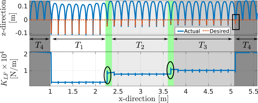
Figure 3.6: Simulation. Traversing multiple terrains of different compliances ($T_{4}$, $T_{1}$, $T_{2}$, $T_{3}$, $T_{4}$). Top: Tracking of the desired terrain penetration of the LF leg in the xz-plane. Bottom: Estimated terrain stiffness of the LF leg. For readability purposes we only plot estimated values less than $2\times 10^{4}$. The green shaded areas highlight the overlap between terrains that results in higher estimated stiffness (black ellipses).

We show the adaptation of STANCE when walking and transitioning between multiple terrains. We test the accuracy of the TCE and the effect of closing the loop of the c³WBC with the TCE on the feet trajectories and terrain penetration. In this simulation, HyQ is traversing five different terrains, starting and ending with a rigid terrain: $T_{4}$, $T_{1}$, $T_{2}$, $T_{2}$, $T_{4}$. The results are presented in Fig. 3.6. The top plot presents the actual foot position against the desired penetration $\epsilon$ of the LF leg in the xz-plane of the world frame. The origin of the z-direction (normal direction) is the uncompressed terrain height. Thus, trajectories below zero represent the penetration of the LF leg. The bottom plot shows the history of the estimated terrain stiffness of the TCE of the LF leg. Table 3.2 reports the mean, standard deviation, and percentage error of the estimated terrain stiffness of the LF leg against the ground truth value set in ODE. The table shows that the TCE had an estimation accuracy below $2$% for the soft terrains $T_{1}$, $T_{2}$ and $T_{3}$. However, the estimation accuracy of the rigid terrain was lower than that of the soft terrains. This is expected since on a rigid terrain, the penetrations are (almost) zero. Thus, a small inaccurate penetration estimation due to any model errors could result in a lower estimation accuracy. Apart from the rigid case, the standard deviation is always below 6$\%$ of the ground truth value. Fig. 3.6 shows that STANCE is always c³, the actual foot position is always consistent with the desired penetration during stance. We can see that, when HyQ is standing over rigid terrain, both the actual foot position and desired penetration are zero. As HyQ walks, over the soft terrains, the penetration is highest in the softest terrain and smallest in the stiffest terrain.

In the simulation environment, we overlapped the terrains to prevent the feet from getting stuck between them. This overlap created a transition (highlighted in green in the figure) which resulted in a stiffer terrain. The overlap was captured by the TCE and resulted in a slight increase in the estimated parameters as highlighted by the two ellipses in the lower plot. We also noticed a lag in estimation, due to a filtering effect, since the TCE is using the most recent $m$-samples. As highlighted by the black box in Fig. 3.6, HyQ was on rigid terrain (actual penetration is zero) while STANCE still perceived it as being on $T_{3}$ (desired penetration is non-zero).

Table 3.2: Mean $\mu$ [N/m], Standard Deviation $\sigma$ [N/m], and Percentage Error of the Estimated Terrain Stiffness of the LF Leg in Simulation.

Terrain	Actual Stiffness	Mean $\mu$ $\pm$ STD $\sigma$	% Error
$T_{1}$	3500	3530 $\pm$ 200	0.9%
$T_{2}$	8000	8110 $\pm$ 400	1.4%
$T_{3}$	10000	10110 $\pm$ 400	1.1%
$T_{4}$	2000000	2240000 $\pm$ 740000	12%

3.7.1.3   Aggressive trunk maneuvers

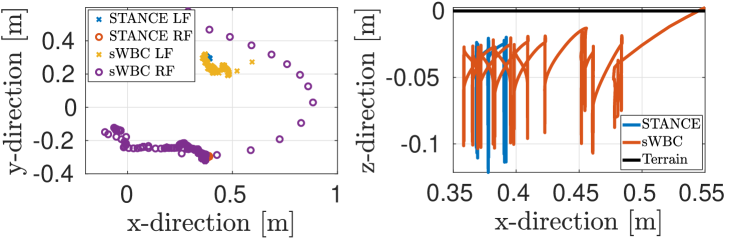
Figure 3.7: Simulation. Comparing sWBC and STANCE under aggressive trunk maneuvers. Left: Top view of the front feet (RF and LF) positions. Right: Side view of the LF position.

We tested sWBC and STANCE under aggressive trunk maneuvers by commanding desired sinusoidal trajectories at the robot’s height ($0.05$ m amplitude and $1.8$ Hz frequency) and at roll orientation ($0.5$ rad amplitude and $1.5$ Hz frequency) over the soft terrain $T_{1}$. The results are shown in Fig. 3.7. The left plot shows a top view of the actual front feet (LF and Right-Front (RF)) positions in the world frame. The right plot shows a side view of the actual LF foot position in the world frame. We notice that the feet of HyQ are always in contact with the terrain in STANCE which is expected since STANCE is c³. Unlike STANCE, the feet did not remain in contact with the terrain in the sWBC. This is clearly seen in Fig. 3.7 where HyQ lost contact multiple times. This resulted in the robot falling over in the sWBC case as shown in the video.

3.7.1.4   Speed Test

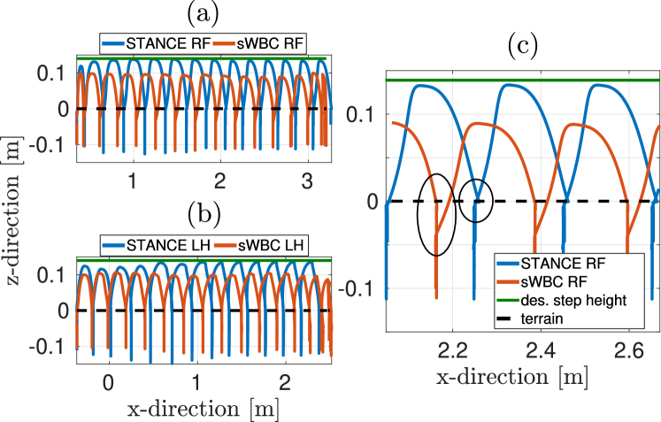
Figure 3.8: Simulation. Speed test. Increasing the desired forward velocity from $0.05$ to $0.3$ m/s. Left: Side view of the RF (a) and LH (b) positions. Right: (c) Closeup section of the top left plot. The green lines are the desired step height. The black dashed lines are the terrain height.

We carried out a simulation where HyQ walks over soft terrain $T_{1}$, starting with a forward velocity of $0.05$ m/s until it reaches $0.3$ m/s with an acceleration of $0.005$ m/s². In this simulation, we compare STANCE against the sWBC. Fig. 3.8a and Fig. 3.8b show the actual trajectories of the RF and Left-Hind (LH) legs in the world frame, respectively. Fig. 3.8c shows a closeup section of the RF leg’s trajectory. The simulation shows that STANCE was c³ over the entire simulation while the sWBC was not.

In particular, STANCE was able to remain in contact with the terrain that allowed HyQ to start the swing phase directly from the terrain height. Unlike STANCE, the sWBC is not terrain aware and did not remain c³ which resulted in starting the swing trajectory while still being inside the deformed terrain. This is highlighted by the two ellipses in the right plot. Additionally, the compliance contact consistency property of STANCE enabled the robot to maintain the desired step clearance (i.e., achieving the desired step height of $0.14$ cm) compared to sWBC. Most importantly, as shown in the accompanying video, the sWBC failed to complete the simulation and could not achieve the final desired forward velocity; It fell at a speed of $0.21$ m/s. Note that both approaches could reach higher velocities with a more dynamic gait (trot). However, this simulation is not focusing on analyzing the maximum speed that the two approaches can reach but rather the differences between these approaches at a higher crawl speeds.

3.7.1.5   Power Test

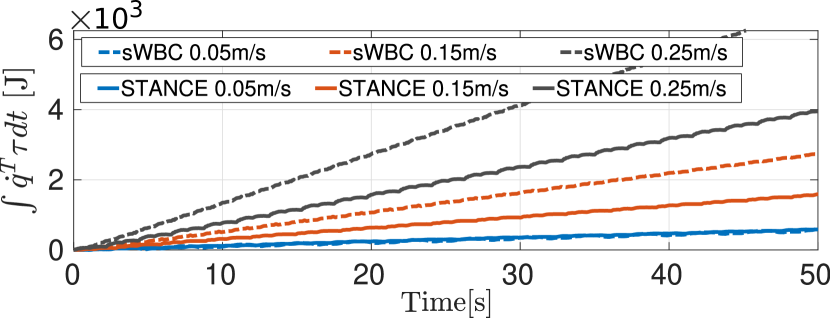
Figure 3.9: Simulation. Power consumption comparison between sWBC and STANCE with different forward velocities (0.05 m/s, 0.15 m/s and 0.25 m/s).

In this test, we compare the power consumption using STANCE and sWBC on HyQ during walking over the soft terrain $T_{1}$ at different forward velocities ($0.05$ m/s, $0.15$ m/s and $0.25$ m/s). Fig. 3.9 presents the energy plots of STANCE and sWBC. The plot shows that STANCE requires less power than the sWBC because it knows how the terrain will deform. STANCE exploits the terrain interaction to achieve the motion. The difference in consumed energy is negligible at $0.05$ m/s but becomes significant at higher speeds.

3.7.2   Experiment

We validated the simulation presented in Section 3.7.1 on the real platform. We analyzed sWBC, c³WBC (with fixed terrain parameters) and STANCE as well as the performance of the TCE module itself.

A foam block of $160$ cm $\times~{}120$ cm $\times~{}20$ cm was selected as a soft terrain for these experiments. To obtain a ground truth of the foam stiffness, we carried out indentation tests on a $50$ cm³ sample of the foam with a stress-strain machine that covers the range of penetration of interest for our robot (below $0.15$ cm). The indentation test showed a softening behavior of the foam with an average stiffness of $2400$ N/m. The MAE of the GRFs of the upcoming experiments are shown in Table 3.3.

3.7.2.1   Locomotion over Soft Terrain

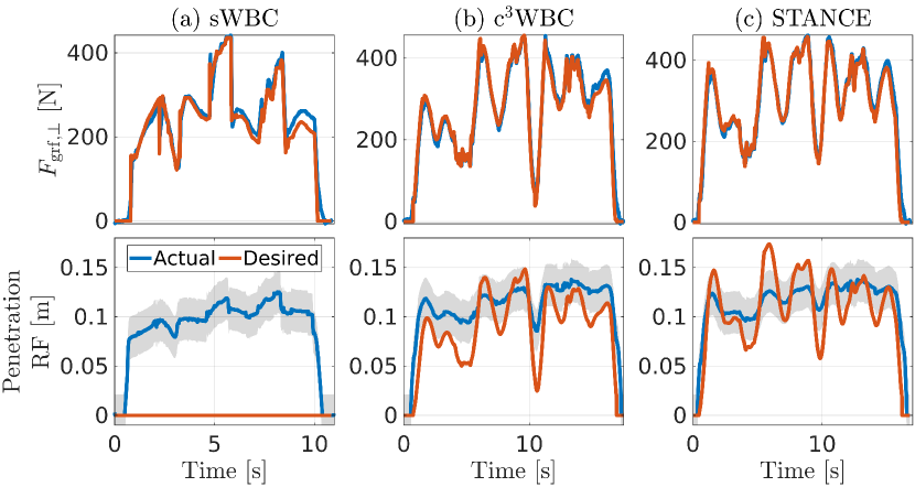
Figure 3.10: Experiment. Comparing sWBC, c³WBC and STANCE over a soft foam block ($K_{t}=2400$ N/m). Top: Tracking of the GRFs of the RF leg. Bottom: Tracking of the foot penetration. The gray shaded areas represent the uncertainty of the measurements.

Table 3.3: Mean Absolute Tracking Error (MAE) [N] of the GRFs using sWBC, c³WBC and STANCE under Different Sets of Experiments.

Description	sWBC	c3WBC	STANCE
Soft Terrain (Sec. 3.7.2.1)	73.9042	68.5581	61.8207
Longitudinal Trans. (Sec. 3.7.2.2)	70.5276	64.2636	60.6285
Lateral Trans. (Sec. 3.7.2.3)	73.0766	-	53.0107

Table 3.4: Mean $\mu$ [N/m], Standard Deviation $\sigma$ [N/m], and Percentage Error of the Estimated Terrain Stiffness of the Four Legs in Experiment over Soft Terrain ($2400$ N/m).

Leg	Mean $\mu$ $\pm$ STD $\sigma$	% Error
LF	2186 $\pm$ 166	9%
RF	2731 $\pm$ 173	14%
LH	2368 $\pm$ 317	1%
RF	2078 $\pm$ 331	13%

In this experiment, HyQ is walking over the foam with a forward velocity of $0.07$ m/s using the three approaches. The results are presented in Fig. 3.10 that shows the actual and desired $F_{\mathrm{grf,\perp}}$ and penetration of the RF leg. The shaded gray area in the lower plots of Fig. 3.10 represents the uncertainty in the estimation of the foot position (see Section 3.6.1). In these experiments, all three approaches performed well; none of them failed. However, the shape of GRFs were different within the three approaches. As in Section 3.7.1.1, since sWBC is rigid contact consistent, the desired GRFs were designed for rigid contacts. Unlike sWBC, STANCE is c³, which was capable of changing the shape of the GRFs. This is highlighted in Table 3.3 in which STANCE outperformed sWBC in the tracking of the GRFs.

In simulation, when we provided the c³WBC with the true value of the stiffness, the MAE of the GRFs was better. However, in this experiment, providing the value obtained from the indentation tests to the c³WBC resulted in a worse GRFs MAE. This outperformance of STANCE compared to the c³WBC in this experiment could be because of the TCE. To clarify, the actual terrain compliances are not constant, but since the TCE is online, it is able to capture these changes in the terrain compliances as well as model errors. As shown in the accompanying video, STANCE had a smoother transition during crawling compared to sWBC. We found the robot transitioning from swing to stance more aggressively in sWBC than STANCE. Such smooth behavior was also noticed in [49].

Table 3.4 shows the mean, standard deviation, and percentage error of the estimated terrain stiffness of all the four legs against the ground truth value ($2400$ N/m) obtained from the indentation tests. The table shows that the accuracy of the TCE in simulation is better than in experiments. This is expected since in simulation, the TCE has a perfect knowledge of the feet penetration. However, the accuracy of our TCE is better compared to [13] in which the percentage error exceeded 50% (the actual stiffness was more than double that of the estimated one in [13]).

3.7.2.2   Longitudinal Transition Between Multiple Terrains

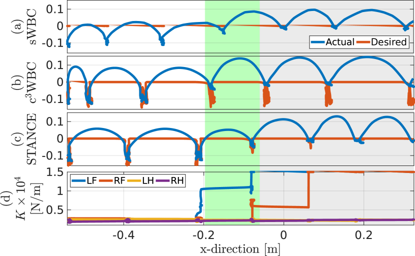
Figure 3.11: Experiment. Longitudinal transition from soft to rigid terrain. The first three plots show the tracking of the desired foot penetration of RF leg using the three approaches (the sWBC, c³WBC with fixed terrain stiffness and STANCE. The fourth plot shows the stiffness estimated by the TCE for the four legs.

Similar to Section 3.7.1.2, we compare the three approaches while transitioning between the foam block and a rigid pallet. We added a pad between between the two terrains to avoid the foot getting stuck (see Fig. 3.1a). Fig. 3.11a-c show the actual position and the desired penetration of the RF leg in the xz-plane for the three approaches. Fig. 3.11d shows the estimated terrain stiffness of the TCE for all four feet.

From Fig. 3.11a-b we see that both sWBC and c³WBC did not adapt to terrain changes. Since both controllers are designed for a specific constant terrain, the desired penetration did not change from soft to rigid. In the sWBC, there is no tracking of the penetration, and in the c³WBC, the tracking of the penetration is good only when the leg is on the foam where the stiffness is consistent to the one used in the controller. On the other hand, as shown in Fig. 3.11c-d, STANCE changes its parameters when facing a different terrain; it was capable of adapting its desired penetration to the type of terrain. In fact, the desired penetration was non-zero on soft terrain and was almost zero on rigid terrain. This again resulted in STANCE achieving the best GRFs tracking as shown in Table 3.3.

Fig. 3.11d shows the importance of having a TCE for each leg. The estimated terrain parameters are different between the legs where the hind legs are on the foam while the rigid ones transitioning from foam to rigid. The figure also shows that the LF leg walked over the rigid terrain before the RF and that the TCE captures the intermediate stiffness estimation due to the rubber pad (see video).

3.7.2.3   Lateral Transition Between Multiple Terrains

Unlike the previous experiment, we set the foam and the pallet laterally as shown in Fig. 3.1c and in the accompanying video. This is a more challenging scenario for stability reasons. In particular, the robot must extend its leg further in the soft terrain maintain the trunk’s balance. Consequently, since the width of HyQ’s torso is smaller than its length, the Zero Moment Point (ZMP) is more likely to get out of the support polygon. The GRFs MAE in Table 3.3 show that STANCE can outperform sWBC during both longitudinal and lateral transitions.

3.7.2.4   External Disturbances over Soft Terrain

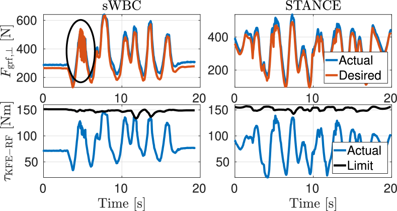
Figure 3.12: Experiment. The sWBC and STANCE under disturbances over soft terrain. Top: The actual and desired $F_{\mathrm{grf,\perp}}$ in sWBC and STANCE, respectively. Bottom: The actual torque and torque limits of the Knee Flexion-Extension (KFE) joint of the RF leg in sWBC and STANCE, respectively.

In this experiment, we test the sWBC and STANCE when the user applies a disturbance on HyQ. The results are shown in Fig. 3.12. The top plots show the actual and desired $F_{\mathrm{grf,\perp}}$ in sWBC and STANCE, respectively. The bottom plots show the actual torque and torque limits of the Knee Flexion-Extension (KFE) joint of the RF leg in sWBC and STANCE, respectively. In the accompanying video, we can qualitatively see that with STANCE, the feet of HyQ keep moving to remain c³ with the terrain. On the other hand, the sWBC kept its feet stationary. This behavior was also reported by [29].

Most importantly, we noticed that HyQ reaches the torque limits in the sWBC as shown in Fig. 3.12. However, in STANCE, since the robot was constantly moving its feet, hence redistributing its forces, the torque limits were not reached. This behavior was also reflected on the GRFs in which, the GRFs were resonating in the sWBC as highlighted by the ellipse in Fig. 3.12.

3.7.2.5   TCE’s Performance over Multiple Terrains

Table 3.5: Mean $\mu$ [N/m] and Standard Deviation $\sigma$ [N/m] of the Estimated Terrain Stiffness of the Four Legs in Experiments (see Fig. 3.1b).

Leg	Mean $\mu$ $\pm$ STD $\sigma$
LF	448400 $\pm$ 165100
RF	55200 $\pm$ 48400
LH	2645000 $\pm$ 336000
RH	1393000 $\pm$ 442000

We analyze the performance of the TCE on HyQ over multiple terrains with various softnesses. The softness of the four used terrains are shown in Fig. 3.1b. The estimated stiffness (mean and standard deviation) under each leg is shown in Table 3.5. As shown in the table, the robot can differentiate between the types of terrain. Although we did not measure the true stiffness value of these terrains, we can observe their softness in the video and Fig. 3.1b and compare it to the values in Table 3.5.

3.7.3   Computational Analysis

STANCE is running online which means that we can estimate the terrain compliance (using the TCE) continuously while walking, and run the entire framework without breaking real-time requirements. We validated the first argument by showing that indeed the TCE can continuously estimate the terrain compliance. Hereafter, we validate the second argument by analyzing the computational complexity of STANCE and compare it against the sWBC. Since our WBC framework is running at $250~{}\mathrm{Hz}$, it is essential that the computation does not exceed the $4~{}\mathrm{ms}$ time frame. Hence, we conducted a simulation in which we calculated the time taken to process the entire framework without the lower level control (ie., the state estimator, the planner and the WBC) that is running on a different real-time thread at $1~{}\mathrm{kHz}$. We compared the computation time on an Intel Core i$7$ quad core CPU in the case of STANCE (the c³WBC and the TCE) and the sWBC. We used the same parameters and gains as in Section 3.7.1.1. The results show that the average processing time taken was $0.68~{}\mathrm{ms}$ and $0.74~{}\mathrm{ms}$ for the sWBC and STANCE respectively. In both cases, the maximum computation time was always below $2~{}\mathrm{ms}$.

3.8  Conclusions

We presented a soft terrain adaptation algorithm called STANCE: Soft Terrain Adaptation aNd Compliance Estimation. STANCE can adapt online to any type of terrain compliance (stiff or rigid). STANCE consists of two main modules: a compliant contact consistent whole-body controller (c³WBC) and a terrain compliance estimator (TCE). The c³WBC extends our previously implemented WBC (sWBC) [1], such that it is contact consistent to any type of compliant terrain given the terrain parameters. The TCE estimates online the terrain compliance and closes the loop with the c³WBC. Unlike previous works on WBC, STANCE does not assume that the ground is rigid. Stance is computationally lightweight and it overcomes the limitations of the previous state of the art approaches. As a result, STANCE can efficiently traverse multiple terrains with different compliances. We validated STANCE on our quadruped robot HyQ over multiple terrains of different stiffness in simulation and experiment. This, to the best of the authors’ knowledge, is the first experimental validation on a legged robot of closing the loop with a terrain estimator.

Incorporating the terrain knowledge makes STANCE c³. This means that STANCE is able to generate smooth GRFs that are physically consistent with the terrain, and continuously adapt the robot’s feet to remain in contact with the terrain. As a result, the tracking error of the GRFs and the power consumption were reduced, and the impact during contact interaction was attenuated. Furthermore, STANCE is more robust in challenging scenarios. As demonstrated, STANCE made it possible to perform aggressive maneuvers and walk at high walking speeds over soft terrain compared to the state of the art sWBC. In the standard case, the contact is lost because the motion of the terrain is not taken into account. On the other hand, there are minor differences in performance between STANCE and the sWBC for less dynamic motions.

STANCE can efficiently transition between multiple terrains with different compliances, and each leg was able to independently sense and adapt to the change in terrain compliance. We also tested the capability of the TCE in discriminating between different terrains. The insights gained in simulation have been confirmed in experiment.

In future works, we plan to implement an algorithm to improve the TCE. In particular, we plan on using onboard sensors, such as a camera, instead of relying on the external measurements from an MCS. We also plan to explore other non-linear contact models in the TCE and the c³WBC.

Chapter 4  On State Estimation
for Legged Locomotion over Soft Terrain

Abstract. Locomotion over soft terrain remains a challenging problem for legged robots. Most of the work done on state estimation for legged robots is designed for rigid contacts, and does not take into account the physical parameters of the terrain. That said, this letter answers the following questions: how and why does soft terrain affect state estimation for legged robots? To do so, we utilized a state estimator that fuses IMU measurements with leg odometry that is designed with rigid contact assumptions. We experimentally validated the state estimator with the HyQ robot trotting over both soft and rigid terrain. We demonstrate that soft terrain negatively affects state estimation for legged robots, and that the state estimates have a noticeable drift over soft terrain compared to rigid terrain.

4.1  Introduction

Quadruped robots are advancing towards being fully autonomous as can be seen by their recent development in research and industry, and their remarkable agile capabilities [74, 75, 76]. This demands quadruped robots to be robust while traversing a wide variety of unexplored complex non-flat terrain. The terrain may not just vary in geometry, but also in its physical properties such as terrain impedance or friction. Reliable state estimation is a major aspect for the success of the deployment of quadruped robots because most locomotion planners and control strategies rely on an accurate estimate of the pose and velocity of the robot. Furthermore, reliable state estimation is essential, not only for locomotion (low-level state estimation), but also for autonomous navigation and inspection tasks that are emerging applications for quadruped robots (task-level state estimation).

To date, most of the work done on state estimation for legged robots are based on filters that fuse multiple sensor modalities. These sensor modalities mainly include high frequency inertial measurements and kinematic measurements (e.g., leg odometry), as well as other low frequency modalities (e.g., cameras and lidars) to correct the drift.

For instance, an Extended Kalman Filter (EKF)-based sensor fusion algorithm has been proposed by [67] that fuses Inertial Measurement Unit (IMU) measurements, leg odometry, stereo vision, and lidar. In [77], a similar algorithm has been proposed that fuses IMU measurements, leg odometry, stereo vision, and GPS. In [75], a nonlinear observer that fuses IMU measurements and leg odometry has been proposed. In [78], a state estimator fuses a Globally Exponentially Stable (GES) nonlinear attitude observer based on IMU measurements with leg odometry to provide bounded velocity estimates. The global stability is important for cases when the robot may have fallen over whereas typical EKF-based works may diverge. The bounded velocity estimates help to decrease drift in the unobservable position estimates. Finally, an approach similar to [78] has been proposed in [79]. This approach proposed an invariant EKF-based sensor fusion algorithm that includes IMU measurements, contact sensor dynamics, and leg odometry.

The aforementioned state estimators are shown to be reliable on stiff terrain. Yet, over soft terrain (as shown in Fig. 4.1), the performance of these state estimators starts to decline. Over soft terrain, the state estimator has difficulties determining when a foot is in contact with the ground. For instance, the state estimator has difficulties determining if the foot is in the air, if the foot is applying more force than the terrain (terrain compression), if the terrain itself is applying more force than the foot (terrain expansion), or if the foot and the terrain are applying the same force (rigid terrain). This results in a large position estimate drift, and it was reported in our previous work [2] where we noted that we encountered difficulties because of state estimation over soft terrain. Apart from our previous work, other works also mention that state estimation over soft terrain is a challenging task, e.g., [80, 46]. Yet, to the authors’ knowledge, literature has not yet discussed the question on how soft terrain affects the state estimation.

The contributions of this work are the experimental analysis and formal study on: the effects of soft terrain on state estimation, the reasons behind these effects, and simple ways to improve state estimation. This letter is building upon our previous work on soft terrain adaptation [2] and on state estimation [78].

The rest of this letter is organized as follows: Section 4.2 describes the robot model, the onboard sensors, and how to estimate the Ground Reaction Forces (GRFs) acting on the robot. Section 4.3 explains the state estimator used in this letter, and how to estimate the base velocity of the robot using leg odometry. Section 4.4 details the results of our experiment and demonstrates how soft terrain affects state estimation. Finally, Section 4.5 presents our conclusions.

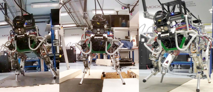
Figure 4.1: HyQ traversing multiple terrains of different compliances.

4.2  Modeling, Sensing, and Estimating

In this letter, we consider the quadruped robot HyQ [66] shown in Fig. 4.1. Each leg has three actuated joints. Despite experimenting on a specific platform, the problem is generic in nature and it applies equally to any legged robot. Furthermore, by using the $90$ kg HyQ robot, a heavy and strong platform, we are exciting more dynamics.

4.2.1   Notations

We introduce the following reference frames: the body frame $\mathcal{B}$ which is located at the geometric center of the trunk (robot torso), and the navigation frame $\mathcal{N}$ which is assumed inertial (world frame). The basis of the body frame are orientated forward, left, and up. To simplify notation, the IMU is located such that the accelerometer measurements are directly measured in $\mathcal{B}$.

4.2.2   Kinematics and Dynamics

Assuming that all of the external forces are exerted on the feet, the dynamics of the robot is

$$M(\bar{x})\ddot{\bar{x}}+h(\bar{x},\dot{\bar{x}})=\bar{\tau}$$ (4.1)

where $\bar{x}=\begin{bmatrix}x^{T}&\eta^{T}&q^{T}\end{bmatrix}^{T}\in\mathbb{R}^{18}$ is the generalized robot states, $\dot{\bar{x}}\in\mathbb{R}^{18}$ is the corresponding generalized velocities, $\ddot{\bar{x}}\in\mathbb{R}^{18}$ is the corresponding generalized accelerations, $x\in\mathbb{R}^{3}$ is the position of the base, $\eta\in\mathbb{R}^{3}$ is the attitude of the base, $q\in\mathbb{R}^{12}$ is the vector of joint angles of the robot, $M\in\mathbb{R}^{18\times 18}$ is the joint-space inertia matrix, $h$ is the vector of Coriolis, centrifugal and gravity forces, $\bar{\tau}=(\begin{bmatrix}0&\tau^{T}\end{bmatrix}^{T}-JF)\in\mathbb{R}^{18}$, $\tau\in\mathbb{R}^{12}$ is the vector of actuated joint torques, $J\in\mathbb{R}^{18\times 12}$ is the floating base Jacobian, and $F\in\mathbb{R}^{12}$ is the vector of external forces (i.e., GRFs).

We solve for the GRFs $F_{\ell}$ of each leg $\ell$ using the actuated part of the dynamics in (4.1).

$$F_{\ell}=-\alpha_{\ell}(J_{\ell}^{T}(q_{\ell}))^{-1}(\tau_{\ell}-h_{\ell}(\bar{x}_{\ell},\dot{\bar{x}}_{\ell}))$$ (4.2)

$F_{\ell}\in\mathbb{R}^{3}\subset F$ is the GRFs for $\ell$ in $\mathcal{B}$, $J_{\ell}\in\mathbb{R}^{3\times 3}\subset J$ is the foot Jacobian of $\ell$, $\tau_{\ell}\in\mathbb{R}^{3}\subset\tau$ is the vector of joint torques of $\ell$, $h_{\ell}\in\mathbb{R}^{3}\subset h$ is the vector of centrifugal, Coriolis, gravity torques of $\ell$ in $\mathcal{B}$, and $\alpha_{\ell}\in\{0,1\}$ selects if the foot is on the ground or not. A threshold of $F_{\ell}$ is typically used to calculate $\alpha_{\ell}$.

$$\alpha_{\ell}=\begin{cases}1&||(J_{\ell}^{T})^{-1}(\tau_{\ell}-h_{\ell})||>\epsilon\\ 0&\text{otherwise}\end{cases}$$ (4.3)

where $\epsilon>0\in\mathbb{R}$ is the threshold.

Assumption 4.1

There exists a force threshold $\epsilon$ that determines if the foot is in contact with the environment.

The translational and rotational kinematics, and the translational dynamics of the robot as a single rigid body in $\mathcal{N}$ are

$$\dot{x}^{n}=v^{n} \dot{v}^{n}=a^{n}+g^{n} \dot{R}^{n}_{b}=R^{n}_{b}S(\omega^{b})$$ (4.4)

where $x^{n}\in\mathbb{R}^{3}$, $v^{n}\in\mathbb{R}^{3}$, $a^{n}\in\mathbb{R}^{3}$ are the position, velocity, and acceleration of the base in $\mathcal{N}$, respectively, $R_{b}^{n}\in\operatorname{SO}(3)$ is the rotation matrix from $\mathcal{B}$ to $\mathcal{N}$, and $\omega^{b}$ is the angular velocity of the base in $\mathcal{B}$. The skew symmetric matrix function is $S()$.

4.2.3   Sensors

The modeling assumes that the quadruped robot is equipped with a six-axis IMU on the trunk (3 Degrees of Freedom (DoFs) gyroscope and 3 DoFs accelerometer), and that every joint contains an encoder and a torque sensor. The accelerometer measures specific force $f_{s}^{b}\in\mathbb{R}^{3}$

$$f_{s}^{b}=a^{b}+g^{b}$$ (4.5)

where $a^{b}\in\mathbb{R}^{3}$ is the acceleration of the body in $\mathcal{B}$ and $g^{b}\in\mathbb{R}^{3}$ is the acceleration due to gravity in $\mathcal{B}$. The gyroscope directly measures angular velocity $\omega^{b}\in\mathbb{R}^{3}$ in $\mathcal{B}$. The encoders are used to measure the joint position $q_{i}\in\mathbb{R}$ and joint speed $\dot{q}_{i}\in\mathbb{R}$. The pose of each joint (i.e., the forward kinematics) is assumed to be exactly known. The torque sensors in the joints directly measure torque $\tau_{i}\in\mathbb{R}$.

The measured values of all of the sensors differ from the theoretical values in that they contain a bias and noise: $\tilde{x}=x+b_{x}+n_{x}$ where $\tilde{x}$, $b_{x}$, and $n_{x}$ are the measured value, bias, and noise of $x$, respectively. All of the biases are assumed to be constant or slowly time-varying, and all of the noise variables have zero mean and a Gaussian distribution.

4.3  State Estimator

To compare the effect of different terrains, we use the state-of-the-art low-level state estimator from [78]. It includes input from three proprioceptive sensors: an IMU, encoders, and torque sensors. For reliability and speed no exteroceptive sensors are used. The state estimator consists of three major components: an attitude observer, leg odometry, and a sensor fusion algorithm.

4.3.1   Non-linear Attitude Observer

Typically in the quadruped robot literature an EKF is used for attitude estimation, e.g., [67, 77, 81]. However, our attitude observer [78] is GES, and it consists of a Non-Linear Observer (NLO) [82] and an eXogeneous Kalman Filter (XKF) [83]. The NLO is

$$\begin{split}\dot{\hat{R}}^{n}_{b}&=\hat{R}^{n}_{b}S(\omega^{b}-\hat{b}^{b})+\sigma K_{p}J_{s}(\hat{R}^{n}_{b})\\ \dot{\hat{b}}^{b}&=\operatorname{Proj}\left(\hat{b}^{b},-k\operatorname{vex}\left(\mathbb{P}\left({\hat{R}^{nT}_{bs}}K_{p}J_{s}(\hat{R}^{n}_{b})\right)\right)\right)\\ J_{s}(\hat{R}^{n}_{b})&=\sum_{j=1}^{k}(y_{j}^{n}-\hat{R}^{n}_{b}y_{j}^{b}){y_{j}^{b}}^{T}\end{split}$$ (4.6)

where $K_{p}\in\mathbb{R}^{3\times 3}$ is a symmetric positive-definite gain matrix, $k>0\in\mathbb{R}$ is a scalar gain, $\sigma\geq 1\in\mathbb{R}$ is a scaling factor, $\hat{R}^{n}_{bs}=\operatorname{sat}(\hat{R}^{n}_{b})$, the function $\operatorname{sat}(X)$ saturates every element of $X$ to $\pm 1$, $\operatorname{Proj}$ is a parameter projection that ensures that $||\hat{b}||<M_{b}$, $M_{b}>0\in\mathbb{R}$ is a constant known upper bound on the gyro bias, $\mathbb{P}(X)=\frac{1}{2}(X+X^{T})$ for any square matrix $X$, and $J_{s}$ is the stabilizing injection term. The observer is GES for all initial conditions assuming there exists $k>1$ non-collinear vector measurements, i.e., $\left|y_{i}^{n}\times y_{j}^{n}\right|>0$ where $i,j\in\{1,\cdots,k\}$. Furthermore, if there is only one measurement the observer is still GES if the following Persistency of Excitation (PE) condition holds: if there exist constants $T>0\in\mathbb{R}$ and $\gamma>0\in\mathbb{R}$ such that, for all $t\geq 0$, $\int_{t}^{t+T}y_{1}^{n}(\tau)y_{1}^{n}(\tau)^{T}\mathop{d\tau}\geq\gamma I$ holds then $y_{1}^{n}$ is PE. See [82] for proof.

The XKF [83] is similar to an EKF in that it linearizes a nonlinear model about an estimate of the state and then applies the typical Linear Time-Varying (LTV) Kalman filter to the linearized model. If the estimate is close to the true state then the filter is near-optimal. However, if the estimate is not close to the true state, the filter can quickly diverge. To overcome this problem, the XKF linearizes about a globally stable exogenous signal from a NLO. The cascaded structure maintains the global stability properties from the NLO and the near-optimal properties from the Kalman filter. The observer is

$$\begin{split}\dot{\hat{x}}&=f_{x}+C(\hat{x}-\breve{x})+K\left(z-h_{x}-H(\hat{x}-\breve{x})\right)\\ \dot{P}&=CP+PC^{T}-KHP+Q\\ K&=PH^{T}R^{-1}\end{split}$$ (4.7)

where $C=\left.\partial f_{x}/\partial{x}\right|_{\breve{x},u}$, $H=\left.\partial h_{x}/\partial{x}\right|_{\breve{x},u}$, $\breve{x}\in\mathbb{R}^{n}$ is the bounded estimate of $x$ from the globally stable NLO. See [83] for the stability proof.

4.3.2   Leg Odometry

Leg odometry computes the overall base velocity $\dot{x}^{b}$ of the robot by combining the contribution of each foot velocity $\dot{x}_{\ell}^{b}$. Each leg $\ell$ only contributes to the leg odometry when it is in contact $\alpha_{\ell}$. Thus, we calculate the overall base velocity $\dot{x}^{b}$ as

$$\dot{x}_{\ell}^{b}=-\alpha_{\ell}\left(J_{\ell}(q_{\ell})\dot{q}-\omega^{b}\times x_{\ell}^{b}\right)\hskip 20.0pt\dot{x}^{b}=\dfrac{1}{n_{s}}\sum_{\ell}\dot{x}_{\ell}^{b}$$ (4.8)

where $n_{s}=\sum\limits_{\ell}\alpha_{\ell}$ is the number of stance legs.

Assumption 4.2

The leg odometry assumes that the robot is always in rigid contact with the terrain. This implies that the stance feet do not move in $\mathcal{N}$, there is no slippage, the terrain does not expand or compress, and the robot does not jump or fly.

4.3.3   Sensor Fusion

Lastly, the inertial measurements (4.5) are fused with the leg odometry (4.8). The main advantage of decoupling the attitude from the position and linear velocity is that the resulting dynamics is LTV, and thus has guaranteed stability properties. i.e., the filter will not diverge in finite time.

We use a LTV Kalman filter with the dynamics (4.4), the accelerometer (4.5), and leg odometry (4.8).

$$\begin{split}\dot{\hat{\underline{x}}}&=f_{\underline{x}}+\underline{K}(\underline{z}-h_{\underline{x}})\\ \dot{\underline{P}}&=\underline{CP}+\underline{PC^{T}}-\underline{K}\underline{H}\underline{P}+\underline{Q}\\ \underline{K}&=\underline{P}\underline{H}^{T}\underline{R}^{-1}\end{split}$$ (4.9)

where the state $\underline{x}=\begin{bmatrix}{x^{n}}^{T}&{v^{n}}^{T}\end{bmatrix}^{T}\in\mathbb{R}^{6}$ is position and velocity of the base, the input $u=(R_{b}^{n}f_{s}^{b}-g^{n})\in\mathbb{R}^{3}$ is the acceleration of the base, the measurement $z=R_{b}^{n}x_{\ell}^{b}\in\mathbb{R}^{3}$ is the leg odometry, $\underline{K}\in\mathbb{R}^{6\times 3}$ is the Kalman gain, $P\in\mathbb{R}^{6\times 6}$ is the covariance matrix, $Q\in\mathbb{R}^{6\times 6}$ is the process noise and $R\in\mathbb{R}^{3\times 3}$ is the measurement noise covariance, and

$$f_{\underline{x}}=\begin{bmatrix}v^{n}\\ u\end{bmatrix}\quad\underline{C}=\begin{bmatrix}0_{3}&I_{3}\\ 0_{3}&0_{3}\end{bmatrix}\quad\underline{H}=\begin{bmatrix}0_{3}&I_{3}\end{bmatrix}$$

and $I_{3}$ and $0_{3}$ are the $3\times 3$ identity matrix and matrix of all zeros, respectively.

4.4  Experimental Results

To analyze the differences in state estimation between rigid and soft terrain, we used HyQ and our state estimator. HyQ has twelve torque-controlled joints powered by hydraulic actuators. HyQ has three types of on board proprioceptive sensors: joint encoders, force/torque sensors, and IMUs. Every joint has an absolute and a relative encoder to measure the joint angle and speed. The absolute encoder (AMS Programmable Magnetic Rotary Encoder - AS5045) measures the joint angle when the robot is first turned on, while the relative encoder (Avago Ultra Miniature, High Resolution Incremental Encoder - AEDA-3300-TE1) measures how far the joint has moved at every epoch. Every joint contains a force or torque sensor. Two joints have a load cell (Burster Subminiature Load Cell - 8417-6005) and one joint has a custom designed torque sensor based on strain-gauges. In the trunk of the robot there is a fibre optic-based, military grade KVH 1775 IMU.

We used the state estimator (4.6)-(4.9) on the Soft Trot in Place and the Rigid Trot in Place dataset from the dataset published in [84]. HyQ was manually controlled to trot on a foam block of $160\times 120\times 20$ cm, and on a rigid ground. An indentation test of the foam shows the foam has an average stiffness of 2400 N/m. All of the sensors were recorded at 1000 Hz. A Motion Capture System (MCS) recorded the ground truth data with millimetre accuracy at 250 Hz.

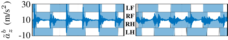
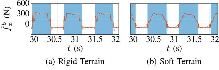
Figure 4.2: The $z$ component of the measured specific force $\tilde{a}_{z}^{b}$ (top), and the estimated ground reaction forces $\hat{f}_{z}^{b}$ (bottom), in the body frame $\mathcal{B}$ of HyQ during a trotting experiment. The highlighted regions show when the given foot is in stance, and the feet are denoted as left-front (LF), right-front (RF), left-hind (LH), and right-hind (RH).

The experiments confirmed our original hypothesis that soft terrain negatively impacts state estimation and also allowed us to investigate why. It is important to note that rigid versus soft terrain had no impact on the attitude estimation. For space reasons, all attitude plots have been omitted.

The first distinct difference between soft and rigid terrain is the specific force measurement of the body as seen in Fig. 4.2. On the rigid terrain there are large impacts and then vibrations every time a foot touches down. Whereas the soft terrain damped out these vibrations. Next, on the soft terrain more prolonged periods of positive and negative acceleration can be seen. This acceleration can also be seen in the plots of the GRFs in Fig. 4.2 where the GRFs on the soft terrain are more continuous when compared to the rigid terrain. In other words, there are longer loading and unloading phases.

The most important differences between soft and rigid terrain are seen in the velocity and position estimates as shown in Fig. 4.3. We can see that the leg odometry has large erroneous peaks in $z$ velocity at both touch-down and lift-off. These peaks in velocities can then be seen in the position estimates as a drift. On the other hand, the $x$ and $y$ position estimates are quite accurate and only have a slow drift.

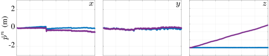
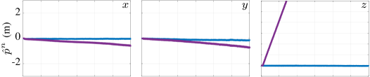
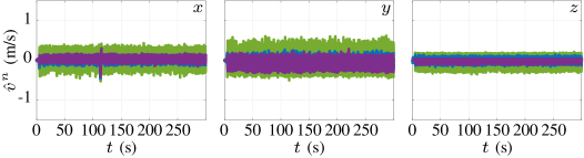
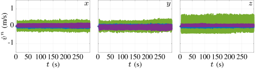
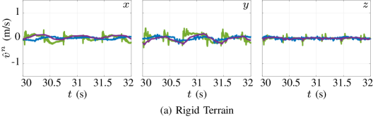
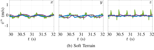
Figure 4.3: The estimated trunk position $\hat{x}^{n}$ (top), and the estimated trunk velocity $\hat{v}^{n}$ (middle and bottom), in the navigation frame $\mathcal{N}$ of HyQ during a trotting experiment using sensor fusion (purple) versus the raw leg odometry (green), and the motion capture system (blue). The first two rows show the full experiment ($0\leq t\leq 300$) s and the bottom row is zoomed in ($30\leq t\leq 32$) s.

In the figures, we can also see multiple of the state estimators assumptions being broken. First, there does not exist a constant $\epsilon$ that can describe when the foot is in contact with the ground, which is contradicting Assumption 4.1. The contact $\epsilon$ is no longer binary (i.e., supporting/not-supporting the weight of the robot), but the contact is now a continuous value with varying amounts of the robot’s weight being supported and sometimes even pushed. When trying to use the previous simple model, the contact ignores a large portion of the loading and unloading phase. Furthermore, it often chatters rapidly between contact/non-contact when the force is close to $\epsilon$. Second, the foot is moving for almost the entire contact (i.e., non-zero acceleration) on soft terrain as shown in Fig. 4.2. This contradicts Assumption 4.2 that the foot velocity is zero when in contact. Third, (4.8) is broken. It assumes that all of the velocity (and all of the acceleration) is a result of the GRFs, but not all of the acceleration due to gravity is being accounted for. Hence, the robot appears to drift up and away from the ground.

There are a few simple ways to try to improve the estimates of this or other similar state estimators. The first is to tune $\epsilon$ in (4.3). By increasing $\epsilon$ there would be less erroneous velocity, but in doing so it would also ignore part of the leg odometry. In general, on a planar surface, a reduced drift in the $z$ direction comes at the cost of an increased error in the $x$ and $y$ directions. A second method could be to have an adaptive velocity bias for the leg odometry. However, the bias is not constant and it depends on both the gait and the terrain. Thus, the problem of estimating the body velocity of the robot using leg odometry remains open.

4.5  Conclusions

In this letter, we present an experimental validation and a formal study on the influence of soft terrain on state estimation for legged robots. We utilized a state-of-the-art state estimator that fuses IMU measurements with leg odometry. We experimentally analyzed the differences between soft and rigid terrain using our state estimator and a dataset of the HyQ robot. That said, we report three main outcomes. First, we showed that soft terrain results in a larger drift in the position estimates, and larger errors in the velocity estimates compared to rigid terrain. These problems are caused by the broken legged odometry contact assumptions on soft terrain. Second, we also showed that over soft terrain, the contact with the terrain is no longer binary and it often chatters rapidly between contact and non-contact. Third, we showed that soft terrain affects many states besides the robot pose. This includes the contact state and the GRFs which are essential for the control of legged robots. Future works include extending the state estimator to incorporate the terrain impedance in the leg odometry model. Additionally, further datasets will be recorded to investigate the long-term drift in the forward and lateral directions.

Part II    Exteroceptive Terrain-Aware Locomotion

Chapter 5  ViTAL:
Vision-Based Terrain-Aware Locomotion
for Legged Robots

Abstract. This work is on vision-based planning strategies for legged robots that separate locomotion planning into foothold selection and pose adaptation. Current pose adaptation strategies optimize the robot’s body pose relative to given footholds. If these footholds are not reached, the robot may end up in a state with no reachable safe footholds. Therefore, we present a Vision-Based Terrain-Aware Locomotion (ViTAL) strategy that consists of novel pose adaptation and foothold selection algorithms. ViTAL introduces a different paradigm in pose adaptation that does not optimize the body pose relative to given footholds, but the body pose that maximizes the chances of the legs in reaching safe footholds. ViTAL plans footholds and poses based on skills that characterize the robot’s capabilities and its terrain-awareness. We use the 90 kg HyQ and 140 kg HyQReal quadruped robots to validate ViTAL, and show that they are able to climb various obstacles including stairs, gaps, and rough terrains at different speeds and gaits. We compare ViTAL with a baseline strategy that selects the robot pose based on given selected footholds, and show that ViTAL outperforms the baseline.

Accompanying Video. https://youtu.be/b5Ea7Jf6hbo

5.1  Introduction

Legged robots have shown remarkable agile capabilities in academia [85, 86, 74, 87, 75, 88] and industry [89, 90, 91]. Yet, to accomplish breakthroughs in dynamic whole-body locomotion, and to robustly traverse unexplored environments, legged robots have to be terrain aware. Terrain-Aware Locomotion (TAL) implies that the robot is capable of taking decisions based on the terrain [92]. The decisions can be in planning, control, or in state estimation, and the terrain may vary in its geometry and physical properties [93, 3, 10, 21, 94, 2, 95, 20, 13]. TAL allows the robot to use its on-board sensors to perceive its surroundings and act accordingly. This work is on vision-based TAL planning strategies that plan the robot’s motion (body and feet) based on the terrain information that is acquired using vision (see Fig. 5.1).

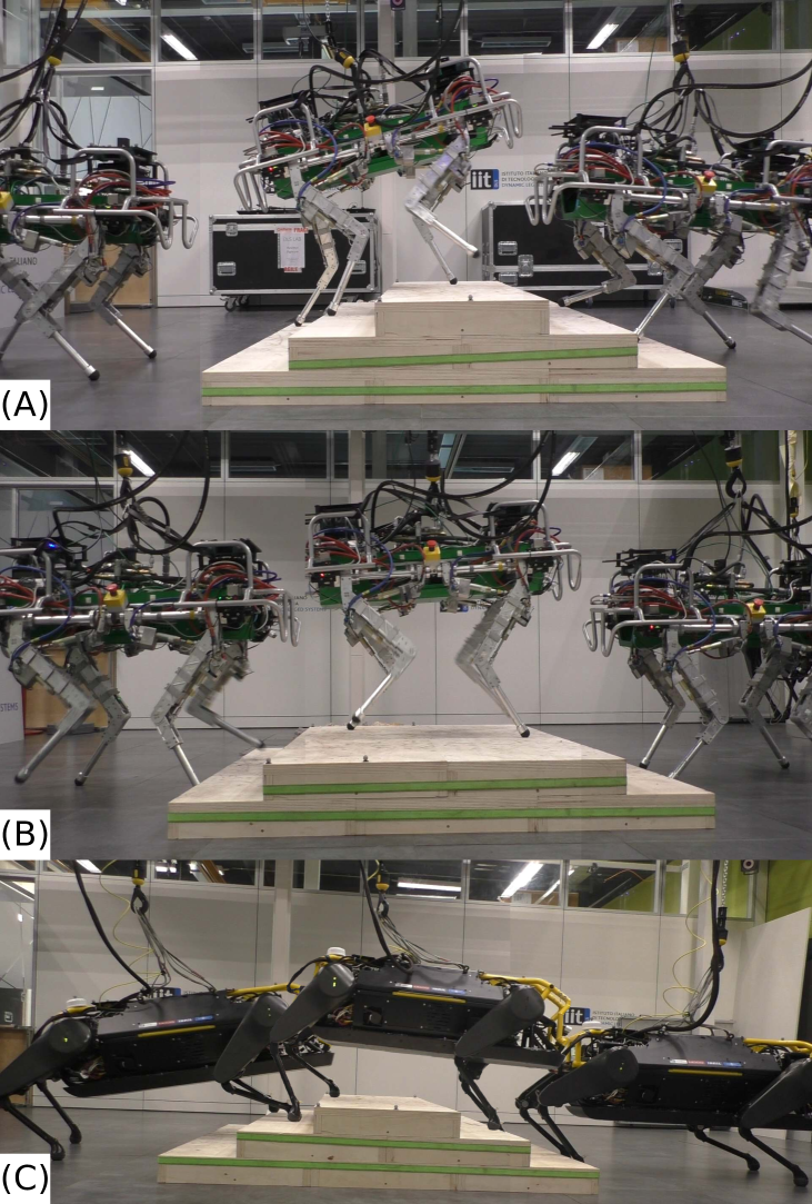
Figure 5.1: The HyQ and HyQReal quadruped robots climbing stairs using ViTAL.

5.1.1   Related Work - Vision-Based Locomotion Planning

Vision-based locomotion planning can either be coupled or decoupled. The coupled approach jointly plans the body pose and footholds in a single algorithm. The decoupled approach independently plans the body pose and footholds in separate algorithms. The challenge in the coupled approach is that it is computationally expensive to solve in real-time. Because of this, the decoupled approach tends to be more practical since the high-dimensional planning problem is split into multiple low-dimensional problems. This also makes the locomotion planning problem more tractable. However, this raises an issue with the decoupled approach because the plans may conflict with each other since they are planned separately. Note that both approaches could be solved using optimization, learning, or heuristic methods.

Trajectory Optimization (TO) is one way to deal with coupled vision-based locomotion planning. By casting locomotion planning as an optimal control problem, TO methods can optimize the robot’s motion while taking into account the terrain information [96, 97, 98, 99, 100]. The locomotion planner can generate trajectories that prevent the robot from slipping or colliding with the terrain by encoding the terrain’s shape and friction properties in the optimization problem [100]. TO methods can also include a model of the terrain as a cost map in the optimization problem, and generate the robot’s trajectories based on that [101]. TO methods provide guarantees on the optimality and feasibility of the devised motions, albeit being computationally expensive; performing these optimizations in real-time is still a challenge. To overcome this issue, TO approaches often implement hierarchical (decoupled) approaches. Instead of decoupling the plan into body pose and footholds, the hierarchical approaches decouple the plan into short and long-horizon plans [102, 103]. Additionally, other work relies on varying the model complexity to overcome the computational issue with TO [104].

Reinforcement Learning (RL) methods mitigate the computational burden of TO methods by training function approximators that learn the locomotion plan [105, 106, 107, 108, 109, 110, 111]. Once trained, an RL policy can generate body pose and foothold sequences based on proprioceptive and/or visual information. Yet, RL methods may require tedious learning (large amounts of data and training time) given its high-dimensional state representations.

As explained earlier, decoupled locomotion planning can mitigate the problems of TO and RL by separating the locomotion plan into feet planning and body planning [112, 113, 114, 115, 116, 117]. Thus, one can develop a more refined and tractable algorithm for every module separately. In this work, planning the feet motion (foothold locations) is called foothold selection, and planning the body motion is called pose adaptation.

5.1.2   Related Work - Foothold Selection and Pose Adaptation

Foothold selection strategies choose the best footholds based on the terrain information and the robot’s capabilities. Early work on foothold selection was presented by Kolter et al. [15] and Kalakrishnan et al. [16] where both approaches relied on motion capture systems and an expert user to select (label) the footholds. These works were then extended in [17] using unsupervised learning, on-board sensors, and considered the terrain information such as the terrain roughness (to avoid edges and corners) and friction (to avoid slippage). Then, Barasuol et al. [18] extended the aforementioned work by selecting footholds that not only considers the terrain morphology, but also considering leg collisions with the terrain. Further improvements in foothold selection strategies added other evaluation criteria such as the robot’s kinematic limits. These strategies use optimization [113, 118, 119], supervised learning [114, 120, 121], RL [85, 95], or heuristic [122] methods.

Similar to foothold selection, pose adaptation strategies optimize the robot’s body pose based on the terrain information and the robot’s capabilities. An early work on vision-based pose adaptation was presented in [112]. The goal was to find the optimal pose that maximizes the reachability of given selected footholds, avoid collisions with the terrain, and maintain static stability. The given footholds are based on a foothold selection algorithm that considers the terrain geometry. Another approach was presented in [123] that finds the optimal body elevation and inclination given the selected footholds, and the robot location in the map. The pose optimizer maximizes different margins that increase the kinematic reachability of the legs and static stability, and avoids terrain collisions. This approach was then extended in [124] with an improved version of the kinematic margins. A similar approach was presented in [113] where the goal was to find an optimal pose that can maximize the reachability of given selected footholds. The reachability term is accounted for in the cost function of the optimizer by penalizing the difference between the default foothold position and the selected one. The work in [115] builds on top of the pose optimizer of [113] to adapt the pose of the robot in confined spaces using 3D terrain maps. This is done using a hierarchical approach that first samples body poses that allows the robot to navigate through confined spaces, then smooths these poses using a gradient descent method that is then augmented with the pose optimizer of [113]. The work presented in [125] generates vision-based pose references that also rely on given selected footholds to estimate the orientation of the terrain and send it as a pose reference. Alongside the orientation reference, the body height reference is set at a constant vertical distance (parallel to gravity) from the center of the approximated plane that fits through the selected footholds.

The aforementioned pose adaptation strategies focus on finding one optimal solution based on given footholds; footholds have to be first selected and given to the optimizer. Despite selecting footholds that are safe, there are no guarantees on what would happen during execution if the footholds are not reached or if the robot deviates from its planned motion. If any of these cases happen, the robot might end up in a pose where no safe footholds can be reached. This would in turn compromise the safety and performance of the robot. Even if the strategy can re-plan, reaching a safe pose might not be possible if the robot is already in an unsafe state.

5.1.3   Proposed Approach

We propose Vision-Based Terrain-Aware Locomotion (ViTAL), an online whole-body locomotion planning strategy that consists of a foothold selection and a pose adaptation algorithm. The foothold selection algorithm used in this work is an extension of the Vision-Based Foothold Adaptation (VFA) algorithm of the previous work done by Villarreal et al. [114] and Esteban et al. [121]. Most importantly, we propose a novel Vision-Based Pose Adaptation (VPA) algorithm that introduces a different paradigm to overcome the drawbacks of the state-of-the-art pose adaptation methods. Instead of finding body poses that are optimal for given footholds, we propose finding body poses that maximize the chances of reaching safe footholds in the first place. Hence, we are interested in putting the robot in a state in which if it deviates from its planned motion, the robot remains around a set of footholds that are still reachable and safe. The notion of safety emerges from skills that characterize the robot’s capabilities.

ViTAL plans footholds and body poses by sharing the same robot skills (both for the VPA and the VFA). These skills characterize what the robot is capable of doing. The skills include, but are not limited to: the robot’s ability to avoid edges, corners, or gaps (terrain roughness), the robot’s ability to remain within the workspace of the legs during the swing and stance phases (kinematic limits), and the robot’s ability to avoid colliding with the terrain (leg collision). These skills are denoted by Foothold Evaluation Criteria (FEC). Evaluating the FEC is usually computationally expensive. Thus, to incorporate the FEC in ViTAL, we rely on approximating them with Convolutional Neural Networks (CNNs) that are trained via supervised learning. This allows us to continuously adapt both the footholds and the body pose. The VFA and the VPA are decoupled and can run at a different update rate. However, they are non-hierarchical, they run in parallel, and they share the same knowledge of the robot skills (the FEC). By that, we overcome the limitations that result from hierarchical planners as mentioned in [115], where high-level plans may conflict with the low-level ones causing a different robot behavior.

The VPA utilizes the FEC to approximate a function that provides the number of safe footholds for the legs. Using this function, we cast a pose optimizer which solves a non-linear optimization problem that maximizes the number of safe footholds for all the legs subject to constraints added to the robot pose. The pose optimizer is a key element in the VPA since it adds safety layers and constraints to the learning part of our approach. This makes our approach more tractable which mitigates the issues that might arise from end-to-end policies in RL methods.

5.1.4   Contributions

ViTAL mitigates the above-mentioned conflicts that exist in other decoupled planners [115, 118, 117, 113]. This is because both the VPA and the VFA share the same skills encoded in the FEC. In other words, the VPA and the VFA will not plan body poses and footholds that may conflict with each other because both planners share the same logic. In this work, the formulation of the VPA allows ViTAL to reason about the leg’s capabilities and the terrain information. However, the formulation of the VPA could be further augmented by other body-specific skills. For instance, the VPA could be reformulated to reason about the body collisions with the environment similar to the work in [117, 126]. The paradigm of the FEC can also be further augmented to consider other skills. We envision that some skills are best encoded via heuristics while others are well suited through optimization. For this reason, the FEC can also handle optimization-based foothold objectives such as the ones in [118].

Following the recent impressive results in RL-based locomotion controllers, we envision ViTAL to be inserted as a module into such control frameworks. To elaborate, current RL-based locomotion controllers [105, 107, 85, 109] are of a single network; the RL framework is a single policy that maps the observations (proprioceptive and exteroceptive) to the actions. This may be challenging since it requires careful reward shaping, and generalizing to new tasks or different sensors (observations) makes the problem harder [127]. For this reason, and similar to Green et al. [127], we envision that ViTAL can be utilized as a planner for RL controllers where the RL controller will act as a reactive controller that then receives guided (planned) commands in a form of optimal poses and footholds from ViTAL.

ViTAL differs from TO and optimization-based methods in several aspects. The FEC is designed to independently evaluate every skill (criterion). Thus, one criterion can be optimization-based while other could be using logic or heuristics. Because of this, ViTAL is not restricted by solving an optimization problem that handles all the skills at once. Another difference between ViTAL and TO is in the way the body poses are optimized. In TO, the optimization problem optimizes a single pose to follow a certain trajectory. The VPA in ViTAL optimizes for the body poses that maximizes the chances of the legs in reaching safe footholds. In other words, the VPA finds a body pose that would put the robot in a configuration where the legs have the maximum possible number of safe footholds. In fact, this paradigm that the VPA of ViTAL introduces may be also encoded in TO. Additionally, TO often finds body poses that considers the leg’s workspace, but to the best of the authors’ knowledge, there is no TO method that finds body poses that consider the legs’ collision with the terrain, and the feasibility of the swinging legs’ trajectory.

To that end, the contributions of this article are

• ViTAL, an online vision-based locomotion planning strategy that simultaneously plans body poses and footholds based on shared knowledge of robot skills (the FEC).

• An extension of our previous work on the VFA algorithm for foothold selection that considers the robot’s body twist and the gait parameters.

• A novel pose adaptation algorithm called the VPA that finds the body pose that maximizes the number of safe footholds for the robot’s legs.

5.2  Foothold Evaluation Criteria (FEC)

The FEC is main the building block for the VFA and the VPA. The FEC are sets of skills that evaluate footholds within heightmaps. The skills include the robot’s ability to assess the terrain’s geometry, avoid leg collisions, and avoid reaching kinematic limits. The FEC can be model-based as in this work and [112, 114], or using optimization techniques as in [113, 118]. The FEC of this work extends the criteria used in our previous work [18, 114, 121].

The FEC takes a tuple $T$ as an input, evaluates it based on multiple criteria, and outputs a boolean matrix $\mu_{\mathrm{safe}}$. The input tuple $T$ is defined as

$$T=(H,z_{h},v_{b},\alpha)$$ (5.1)

where $H\in\mathbb{R}^{h_{x}\times{h_{y}}}$ is the heightmap of dimensions $h_{x}$ and $h_{y}$, $z_{h}\in\mathbb{R}$ is the hip height of the leg (in the world frame), ${v_{b}\in\mathbb{R}^{6}}$ is the base twist, and $\alpha$ are the gait parameters (step length, step frequency, duty factor, and time remaining till touchdown). The heightmap $H$ is extracted from the terrain elevation map, and is oriented with respect to the horizontal frame of the robot [128]. The horizontal frame coincides with the base frame of the robot, and its $xy$-plane is perpendicular to the gravity vector. Each cell (pixel) of $H$ denotes the terrain height that corresponds to the location of this cell in the terrain map. Each cell of $H$ also corresponds to a candidate foothold $p_{c}\in\mathbb{R}^{3}$ for the robot.

In this work, we only consider the following FEC: Terrain Roughness (TR), Leg Collision (LC), Kinematic Feasibility (KF), and Foot Trajectory Collision (FC). Each criterion $C$ outputs a boolean matrix $\mu_{C}$. Once all of the criteria are evaluated, the final output $\mu_{\mathrm{safe}}$ is the element-wise logical AND ($\wedge$) of all the criteria. The output matrix $\mu_{\mathrm{safe}}\in\mathbb{R}^{h_{x}\times{h_{y}}}$ is a boolean matrix with the same size as the input heightmap $H$. $\mu_{\mathrm{safe}}$ indicates the candidate footholds (elements in the heightmap $H$) that are safe. An element in the matrix $\mu_{\mathrm{safe}}$ that is true, corresponds to a candidate foothold $p_{c}$ in the heightmap $H$ that is safe. The output of the FEC is

$$\mu_{\mathrm{safe}}=\mu_{\mathrm{TR}}\wedge\mu_{\mathrm{LC}}\wedge\mu_{\mathrm{KF}}\wedge\mu_{\mathrm{FC}}.$$ (5.2)

An overview of the criteria used in this work is shown in Fig. 5.2(A) and is detailed below.

Terrain Roughness (TR). This criterion checks edges or corners in the heightmap that are unsafe for the robot to step on. For each candidate foothold $p_{c}$ in $H$, we evaluate the mean and standard deviation of the slope relative to its neighboring footholds, and put a threshold that defines whether a $p_{c}$ is safe or not. Footholds above this threshold are discarded.

Leg Collision (LC). This criterion selects footholds that do not result in leg collision with the terrain during the entire gait cycle (from lift-off, during swinging, touchdown and till the next lift-off). To do so, we create a bounding region around the leg configuration that corresponds to the candidate foothold $p_{c}$ and the current hip location. Then, we check if the bounding region collides with the terrain (the heightmap) by measuring the closest distance between them. If this distance is lower than a certain value, then the candidate foothold is discarded.

Kinematic Feasibility (KF). This criterion selects footholds that are kinematically feasible. It checks whether a candidate foothold $p_{c}$ will result in a trajectory that remains within the workspace of the leg during the entire gait cycle. To do so, we check if the candidate foothold $p_{c}$ is within the workspace of the leg during touchdown and next lift-off. Also, we check if the trajectory of the foot from the lift-off position $p_{lo}$ till the touchdown position at the candidate foothold $p_{c}$ is within the workspace of the leg. In the initial implementation in [114], this criterion was only evaluated during touchdown. In this work, we consider this criterion during the entire leg step-cycle.

Foot Trajectory Collision (FC). This criterion selects footholds that do not result in foot trajectory collision with the terrain. It checks whether the foot swing trajectory corresponding to a candidate foothold $p_{c}$ is going to collide with the terrain or not. If the swing trajectory collides with the terrain, the candidate foothold $p_{c}$ is discarded.

Remark 5.1

There are three main sources of uncertainty that can affect the foothold placement [18]. These sources of uncertainty are due to trajectory tracking errors, foothold prediction errors, and drifts in the map. To allow for a degree of uncertainty, after computing $\mu_{\mathrm{safe}}$, candidate footholds that are within a radius of unsafe footholds are also discarded. This is similar to the erosion operation in image processing.

Remark 5.2

The initial implementation of the FEC in [114] only considered the heightmap $H$ as an input; the other inputs of the tuple $T$ in (5.1) were kept constant. This had a few disadvantages that we reported in [121] where we extended the work of [114] by considering the linear body heading velocity. In this work, we build upon that by considering the full body twist $v_{b}$ and the gait parameters $\alpha$ as expressed by $T$ in (5.1).

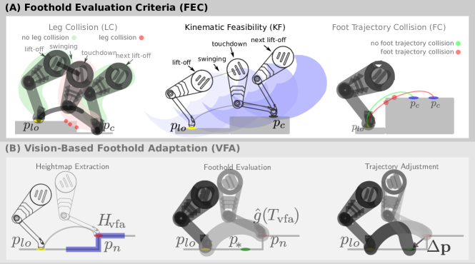
Figure 5.2: Overview of ViTAL. Illustrations are not to scale. (A) The Foothold Evaluation Criteria (FEC): Leg Collision (LC), Kinematic Feasibility (KF), and Foot Trajectory Collision (FC). (B) The Vision-based Foothold Adaptation (VFA) pipeline. First, we extract the heightmap $H_{\mathrm{vfa}}$ around the nominal foothold $p_{n}$. Then, we evaluate the heightmap either using the exact evaluation $g(T_{\mathrm{vfa}})$ or using the CNN as an approximation $\hat{g}(T_{\mathrm{vfa}})$. Once the optimal foothold $p_{*}$ is selected, the swing trajectory is adjusted.

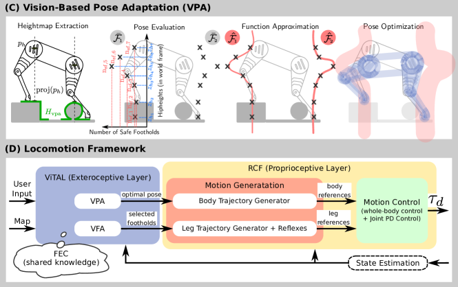
Figure 5.2: Overview of ViTAL (continued). Illustrations are not to scale. (C) The Vision-Based Pose Adaptation (VPA) pipeline. First, we extract the heightmap $H_{\mathrm{vpa}}$ for all the legs. The heightmaps are centered around the projection of the leg hip locations. Then, we evaluate the FEC to compute $\bar{\mathcal{F}}$ for all the hip heights of all the legs (pose evaluation). Then, we approximate a continuous function $\hat{\mathcal{F}}$ from $\bar{\mathcal{F}}$ (function approximation). The pose optimizer finds the pose that maximizes $\hat{\mathcal{F}}$ for all of the legs (pose optimization). (D) Our locomotion framework. ViTAL consists of the VPA and the VFA algorithms. Both algorithms rely on the robot skills which we denote by FEC. $\tau_{d}$ are the desired joint torques that are sent to the robot.

5.3  Vision-Based Foothold Adaptation (VFA)

The VFA evaluates the FEC to select the optimal foothold for each leg [18, 114, 121]. The VFA has three main stages as shown in Fig. 5.2(B): heightmap extraction, foothold evaluation, and trajectory adjustment.

Heightmap Extraction. Using the current robot states and gait parameters, we estimate the touchdown position of the swinging foot in the world frame as detailed in [114]. This is denoted as the nominal foothold $p_{n}\in\mathbb{R}^{3}$. Then, we extract a heightmap $H_{\mathrm{vfa}}$ that is centered around $p_{n}$.

Foothold Evaluation. After extracting the heightmap, we compute the optimal foothold $p_{*}\in\mathbb{R}^{3}$ for each leg. We denote this by foothold evaluation which is the mapping

$$g(T_{\mathrm{vfa}}):T_{\mathrm{vfa}}\rightarrow p_{*}$$ (5.3)

that takes an input tuple $T_{\mathrm{vfa}}$ that is defined as

$$T_{\mathrm{vfa}}=(H_{\mathrm{vfa}},z_{h},v_{b},\alpha,p_{n}).$$ (5.4)

Once we evaluate the FEC in (5.2), from all of the safe candidate footholds in $\mu_{\mathrm{safe}}$, we select the optimal foothold $p_{*}$ as the one that is closest to the nominal foothold $p_{n}$. The aim is to minimize the deviation from the original trajectory and thus results in a less disturbed or aggressive motion. An overview of the foothold evaluation stage is shown in Fig. 5.3 where the tuple $T$ of the FEC in (5.1) is extracted from the VFA tuple $T_{\mathrm{vfa}}$ in (5.4) to compute $\mu_{\mathrm{safe}}$. Then, using $p_{n}$ and $\mu_{\mathrm{safe}}$, we extract $p_{*}$ as the safe foothold that is closest to $p_{n}$.

Trajectory Adjustment. The leg’s swinging trajectory is adjusted once $p_{*}$ is computed.

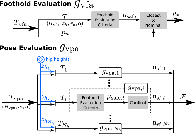
Figure 5.3: Overview of the foothold evaluation stage in the VFA algorithm, and the pose evaluation stage in the VPA algorithm.

Remark 5.3

To compute the foothold evaluation, one can directly apply the exact mapping $g(T_{\mathrm{vfa}})$. Yet, computing the foothold evaluation leads to evaluating the FEC which is generally computationally expensive. Thus, to speed up the computation and to continuously run the VFA online, we train a CNN to approximate the foothold evaluation $\hat{g}(T_{\mathrm{vfa}})$ using supervised learning. Once trained, the VFA can then be executed online using the CNN. The CNN architecture of the foothold evaluation is explained in Section 6.1.

5.4  Vision-Based Pose Adaptation (VPA)

The VPA generates pose references that maximize the chances of the legs to reach safe footholds. This means that the robot pose has to be aware of what the legs are capable of and adapt accordingly. Therefore, the goal of the VPA is to adapt the robot pose based on the same set of skills in the FEC used by the VFA.

5.4.1   Definitions and Notations

Number of Safe Footholds. As explained earlier, the FEC takes a tuple $T$ as an input and outputs the matrix $\mu_{\mathrm{safe}}$. Based on that, let us define the Number of Safe Footholds ($\mathrm{n_{sf}}$)

$$\mathrm{n}_{\mathrm{sf}}:=\mathrm{cardinal}(\{e\in\mu_{\mathrm{safe}}:e=1\})$$ (5.5)

as the number of true elements in the boolean matrix $\mu_{\mathrm{safe}}$.

Set of Safe Footholds. Consider a set of tuples $\mathcal{T}$ where each element $T_{i}\in\mathcal{T}$ is a tuple defined as

$$T_{i}=(H,z_{h_{i}},v_{b},\alpha)$$ (5.6)

and $z_{h_{i}}\in\mathcal{Z}$ is a hip height element in the set of hip heights $\mathcal{Z}$ (in the world frame). All the tuple elements $T_{i}\in\mathcal{T}$ share the same heightmap $H$, body twist $v_{b}$ and gait parameters $\alpha$.

Evaluating the FEC in (5.2) for every $T_{i}\in\mathcal{T}$ that corresponds to $z_{h_{i}}\in\mathcal{Z}$, and computing the cardinal in (5.5) yields $\mathrm{n}_{\mathrm{sf},i}$ for every $T_{i}$. This yields the Set of Safe Footholds ($\mathcal{F}$) which is a set containing the number of safe footholds $\mathrm{n}_{\mathrm{sf}}$ that are evaluated based on the FEC given the set of tuples $\mathcal{T}$ that corresponds to the set of hip heights $\mathcal{Z}$ but shares the same heightmap $H$, body twist $v_{b}$ and gait parameters $\alpha$.

5.4.2   From the Set of Safe Footholds to Pose Evaluation

The set of safe footholds $\mathcal{F}$ is one of the building blocks of the VPA. To compute $\mathcal{F}$, we compute the input tuple $T_{\mathrm{vpa}}$

$$T_{\mathrm{vpa}}=(H_{\mathrm{vpa}},v_{b},\alpha)$$ (5.7)

that we then augment with the hip heights $z_{h_{i}}$ in the hip heights set $\mathcal{Z}$ yielding the set of tuples $\mathcal{T}$. Then, we evaluate the FEC in (5.2) for every $T_{i}\in\mathcal{T}$, and computing the cardinal in (5.5). This can be expressed by the mapping

$${g_{\mathrm{vpa}}(T_{\mathrm{vpa}})~{}:~{}T_{\mathrm{vpa}}\rightarrow\mathcal{F}}$$ (5.8)

which is referred to as pose evaluation. We can express $\mathcal{F}$ as

$$\mathcal{F}=\{\mathrm{n}_{\mathrm{sf},i}=g_{\mathrm{vpa},i}(T_{i})~{}\forall T_{i}\in\mathcal{T}\}.$$ (5.9)

Remark 5.4

Since $\mathcal{Z}$ is an infinite continuous set, so is $\mathcal{F}$ which is not numerically feasible to compute. Hence, we sample a finite set $\bar{\mathcal{Z}}$ of $N_{z_{h}}$ samples of hip heights that results in a finite set of safe footholds $\bar{\mathcal{F}}$. To use the set of safe footholds in an optimization problem, we need a continuous function. Thus, after we compute $\bar{\mathcal{F}}$, we estimate a continuous function $\hat{\mathcal{F}}$ as explained next.

An overview of the pose evaluation is shown in Fig. 5.3 where the tuple $T_{\mathrm{vpa}}$ in (5.7) is augmented with the hip heights $z_{h_{i}}$ from $\bar{\mathcal{Z}}$ to construct the FEC tuples $T_{i}$ in (5.6). For every tuple $T_{i}$, we evaluate the FEC using (5.2) and compute $\mathrm{n}_{\mathrm{sf},i}$ in (5.5) using the mapping in (5.8). Finally, the set $\bar{\mathcal{F}}$ includes all the elements $\mathrm{n}_{\mathrm{sf},i}$ as in (5.9).

5.4.3   Vision-based Pose Adaptation (VPA) Formulation

The VPA has four main stages as shown in Fig. 5.2(C). First, heightmap extraction that is similar to the VFA. Second, pose evaluation where we compute $\bar{\mathcal{F}}$. Third, function approximation where we estimate $\hat{\mathcal{F}}$ from $\bar{\mathcal{F}}$. Fourth, pose optimization where the optimal body pose is computed.

Heightmap Extraction. We extract one heightmap $H_{\mathrm{vpa}}$ per leg that is centered around the projection of the leg’s hip location in the terrain map ($\mathrm{proj.}(p_{h})$ instead of $p_{n}$).

Pose Evaluation. After extracting the heightmaps, we compute $\bar{\mathcal{F}}$ from the mapping in (5.8) of the pose evaluation. In the pose evaluation, the FEC are evaluated for all hip heights in $\bar{\mathcal{Z}}$ given the input tuple $T_{\mathrm{vpa}}$ as shown in Fig. 5.3.

Function Approximation. In this stage, we estimate the continuous function $\hat{\mathcal{F}}$ from $\bar{\mathcal{F}}$, as explained in Remark 5.4. This is done by training a parameterized model of the inputs $T_{i}\in\bar{\mathcal{T}}$ and the outputs $\mathrm{n}_{\mathrm{sf},i}\in\bar{\mathcal{F}}$. The result is the function (model) $\hat{\mathcal{F}}$ that is parameterized by the model parameters $w$. The function approximation is detailed later in this section.

Pose Optimization. Evaluating the FEC and approximating it with the function $\hat{\mathcal{F}}$, introduces a metric that represents the possible number of safe footholds for every leg. Based on this, the goal of the pose optimizer is to find the optimal pose that will maximize the number of safe footholds for every leg (maximize $\hat{\mathcal{F}}$) while ensuring robustness. The pose optimizer is detailed later in this section.

Remark 5.5

Similar to Remark 5.3, one can directly apply the exact evaluation $g_{\mathrm{vpa}}(T_{\mathrm{vpa}})$ for a given $T_{\mathrm{vpa}}$. Yet, since this is computationally expensive, we rely on approximating the evaluation $\hat{g}_{\mathrm{vpa}}(T_{\mathrm{vpa}})$ using a CNN. In fact, the learning part is applied to both the pose evaluation and the function approximation. This means that the pose optimization is running online, outside the CNN. The CNN architecture of the pose evaluation is explained in Section 6.1.

5.4.4   Function Approximation

The goal of the function approximation is to approximate the set of safe footholds $\mathcal{F}$ from the discrete set $\bar{\mathcal{F}}$ computed in the pose evaluation stage. This is done to provide the pose optimizer with a continuous function. Given a dataset $(\bar{\mathcal{Z}},\bar{\mathcal{F}})$ of hip heights $z_{h_{i}}\in\bar{\mathcal{Z}}$ and number of safe footholds ${\mathrm{n}_{\mathrm{sf},i}\in\bar{\mathcal{Z}}}$, the function approximation estimates a function $\hat{\mathcal{F}}(z_{h_{i}},w)$ that is parameterized by the weights $w$. Once the weights $w$ are computed, the function estimate $\hat{\mathcal{F}}(z_{h_{i}},w)$ is then reconstructed and sent to the pose optimizer.

It is important to choose a function $\hat{\mathcal{F}}$ that can accurately represent the nature of the number of safe footholds. The number of safe footholds approaches zero when the hip heights approach $0$ or $\infty$. Thus, we want a function that fades to zero at the extremes (Gaussian-like functions), and captures any asymmetry or flatness in the distribution. Hence, we use radial basis functions of Gaussians. With that in mind, we are looking for the weights $w$

$$w=\text{arg}~{}\text{min}~{}S(w)$$ (5.10)

that minimize the cost $S(w)$

$$S(w)=\sum_{i=1}^{N_{h}}(\mathrm{n}_{\mathrm{sf},i}-\hat{\mathcal{F}}(z_{h_{i}},w))^{2}$$ (5.11)

which is the sum of the squared residuals of $\mathrm{n}_{\mathrm{sf},i}$ and $\hat{\mathcal{F}}(z_{h_{i}},w)$. $N_{h}$ is the number of samples (the number of the finite set of hip heights). The function $\hat{\mathcal{F}}(z_{h_{i}},w)$ is the regression model (the approximation of $\mathcal{F}$) that is parameterized by $w$. The function $\hat{\mathcal{F}}(z_{h_{i}},w)$ is the weighted sum of the basis functions

$$\hat{\mathcal{F}}(z_{h_{i}},w)=\sum_{e=1}^{E}w_{e}\cdot g(z_{h_{i}},\Sigma_{e},c_{e})$$ (5.12)

where $w\in\mathbb{R}^{E}$, and $E$ is the number of basis functions. The basis function is a radial basis function of Gaussian functions

$$g(z_{h_{i}},\Sigma_{e},c_{e})=\text{exp}(-0.5(z_{h_{i}}-c_{e})^{T}\Sigma_{e}^{-1}(z_{h_{i}}-c_{e}))$$ (5.13)

where $\Sigma_{e}$ and $c_{e}$ are the parameters of the Gaussian function. Since the function model in (5.12) is linear in the parameters, the weights of the function approximation can be solved analytically using least squares. In this work, we keep the parameters of the Gaussians ($\Sigma$ and $c$) fixed. Hence, the function $\hat{\mathcal{F}}$ is only parameterized by $w$. For more information on regression with radial basis functions, please refer to [65] and Section 6.2.

5.4.5   Pose Optimization

The pose optimizer finds the robot’s body pose $u$ that maximizes the number of safe footholds for all the legs. This is casted as a non-linear optimization problem. The notion of safe footholds is provided by the function $\hat{\mathcal{F}}(z_{h},w)$ that maps a hip height $z_{h}$ to a number of safe foothold $\mathrm{n_{sf}}$, and is parameterized by $w$. Since the pose optimizer is solving for the body pose $u$, the function $\hat{\mathcal{F}}(z_{h})$ should be encoded using the body pose rather than the hip heights (${\hat{\mathcal{F}}=\hat{\mathcal{F}}(z_{h}(u))}$). This is done by estimating the hip height as a function of the body pose (${z_{h}=z_{h}(u)}$) as shown in Section 6.3.

5.4.6   Single-Horizon Pose Optimization

The pose optimization problem is formulated as

$$\underset{u=[z_{b},\beta,\gamma]}{\text{maximize~{}}} \mathcal{C}(\hat{\mathcal{F}}_{l}(z_{h_{l}}(z_{b},\beta,\gamma)))~{}~{}\forall l\in N_{l}$$ (5.14)

subject to $$u_{\min}\leq u\leq u_{\max}$$ (5.15)

$$\Delta u_{\min}\leq\Delta u\leq\Delta u_{\max}$$ (5.16)

where $u=[z_{b},\beta,\gamma]\in\mathbb{R}^{3}$ are the decision variables (robot body pose) consisting of the robot height, roll and pitch, respectively, $\mathcal{C}$ is the cost function, $\hat{\mathcal{F}}_{l}$ is $\hat{\mathcal{F}}$ for every leg $l$ where $N_{l}=4$ is the number of legs, $z_{h_{l}}\in\mathbb{R}$ is the hip height of the leg $l$, and $u_{\min}$ and $u_{\max}$ are the lower and upper bounds of the decision variables, respectively. $\Delta u=u-u_{k-1}$ is the numerical difference of $u$ where $u_{k-1}$ is the output of $u$ at the previous instant, and $\Delta u_{\min}$ and $\Delta u_{\max}$ are the lower and upper bounds of $\Delta u$, respectively. We can re-write (5.16) as

$$\Delta u_{\min}+u_{k-1}\leq u\leq\Delta u_{\max}+u_{k-1}.$$ (5.17)

The cost function in (5.14) maximizes $\hat{\mathcal{F}}$ for all of the legs. We designed several types of cost functions as detailed next. The constraints in (5.15) and (5.16) ensure that the decision variables and their variations are bounded.

5.4.7   Cost Functions

A standard cost function can be the sum of the squares of $\hat{\mathcal{F}}_{l}$ for all of the legs

$$\mathcal{C}_{\mathrm{sum}}=\sum_{l=1}^{N_{l}=4}\|\hat{\mathcal{F}}_{l}(z_{h_{l}})\|^{2}_{Q}$$ (5.18)

where another option could be the product of the squares of $\hat{\mathcal{F}}_{l}$ for all of the legs

$$\mathcal{C}_{\mathrm{prod}}=\prod_{l=1}^{N_{l}=4}\|\hat{\mathcal{F}}_{l}(z_{h_{l}})\|^{2}_{Q}.$$ (5.19)

The key difference between an additive cost $\mathcal{C}_{\mathrm{sum}}$ and a multiplicative cost $\mathcal{C}_{\mathrm{prod}}$ is that the latter puts equal weighting for each $\hat{\mathcal{F}}_{l}$. This is important since we do not want the optimizer to find a pose that maximizes $\hat{\mathcal{F}}$ for one leg while compromising the other leg(s). One can also define the cost

$$\mathcal{C}_{\mathrm{int}}=\sum_{l=1}^{N_{l}=4}\|\int_{z_{h_{l}}-m}^{z_{h_{l}}+m}\hat{\mathcal{F}}_{l}(z_{h_{l}})~{}dz_{h_{l}}~{}\|^{2}_{Q}$$ (5.20)

which is the sum of squared integrals that can be numerically approximated as

$$\int_{z_{h_{l}}-m}^{z_{h_{l}}+m}\hat{\mathcal{F}}_{l}(z_{h_{l}})~{}dz_{h_{l}}\approx m\cdot(\hat{\mathcal{F}}_{l}(z_{h_{l}}-m)+\hat{\mathcal{F}}_{l}(z_{h_{l}}+m))$$ (5.21)

yielding

$$\mathcal{C}_{\mathrm{int}}=\sum_{l=1}^{N_{l}=4}\|m\cdot(\hat{\mathcal{F}}_{l}(z_{h_{l}}-m)+\hat{\mathcal{F}}_{l}(z_{h_{l}}+m))\|^{2}_{Q}.$$ (5.22)

In this cost option, we do not find the pose that maximizes $\hat{\mathcal{F}}$. Instead, we want to find the pose that maximizes the area around $\hat{\mathcal{F}}$ that is defined by the margin $m$. Using $\mathcal{C}_{\mathrm{int}}$ is important since it adds robustness in case there is any error in the pose tracking during execution. Because of possible tracking errors during execution, the robot might end up in the pose $u^{*}\pm m$ instead of $u^{*}$. If we use $\mathcal{C}_{\mathrm{int}}$ as a cost function, the optimizer will find poses that maximizes the number of safe footholds not just for $u^{*}$ but within a vicinity of $m$. More details on the use of $\mathcal{C}_{\mathrm{int}}$ as a cost function in the pose optimization of the VPA can be found in Section 6.4.

5.4.8   Receding-Horizon Pose Optimization

Adapting the robot’s pose during dynamic locomotion requires reasoning about what is ahead of the robot: the robot should not just consider its current state but also future ones. For that, we extend the pose optimizer to consider the current and future states of the robot in a receding horizon manner. To formulate the receding horizon pose optimizer, instead of considering $\hat{\mathcal{F}}_{l}~{}\forall~{}{l\in N_{l}}$ in the single horizon case, the pose optimizer will consider $\hat{\mathcal{F}}_{l,j}~{}\forall~{}{l\in N_{l}},~{}{j\in N_{h}}$ where $N_{h}$ is the receding horizon number. We compute $\hat{\mathcal{F}}_{l,j}$ in the same way explained in the pose evaluation stage. More details on computing $\hat{\mathcal{F}}_{l,j}$ can be found in Section 6.5.

The receding horizon pose optimization problem is

$$\underset{u=[u_{1}^{T},\cdots,u_{N_{h}}^{T}]}{\text{maximize}} \sum_{j=1}^{N_{h}}\mathcal{C}_{j}(\hat{\mathcal{F}}_{l,j}(z_{h_{l,j}}(u_{j})))$$ (5.23)

$$+ \sum_{j=1}^{N_{h}-1}\|u_{j}-u_{j+1}\|$$

$$\forall l\in N_{l},~{}j\in N_{h}$$

subject to $$u_{\min}\leq u\leq u_{\max}$$ (5.24)

$$\Delta u_{\min}\leq\Delta u\leq\Delta u_{\max}$$ (5.25)

where $u=[u_{1}^{T},\cdots,u_{j}^{T},\cdots,u_{N_{h}}^{T}]\in\mathbb{R}^{3N_{h}}$ are the decision variables during the entire receding horizon $N_{h}$. Each variable $u_{j}=[z_{b,j},\beta_{j},\gamma_{j}]\in\mathbb{R}^{3}$ is the optimal pose of the horizon $j$.

The first term in (5.23) is the sum of the cost functions $\mathcal{C}_{j}$ during the entire horizon ($\forall j\in N_{h}$). The cost $\mathcal{C}_{j}$ can be any of the aforementioned cost functions. The second term in (5.23) penalizes the deviation between two consecutive optimal poses within the receding horizon ($u_{j}$ and $u_{j+1}$). The second term is added so that each optimal pose $u_{j}$ is also taking into account the optimal pose of the upcoming sequence $u_{j+1}$ (to connect the solutions in a smooth way). Similar to the single horizon pose optimizer, $u_{\min}$ and $u_{\max}$ are the lower and upper bounds of the decision variables, respectively. Furthermore, $\Delta u$ denotes the numerical difference of $u$, while $\Delta u_{\min}$ and $\Delta u_{\max}$ are the lower and upper bounds of $\Delta u$, respectively. Note that the constraints of the single horizon and the receding horizon are of different dimensions.

5.5  System Overview

Our locomotion framework that is shown in Fig. 5.2(D) is based on the Reactive Controller Framework (RCF) [128]. ViTAL complements the RCF with an exteroceptive terrain-aware layer composed of the VFA and the VPA. ViTAL takes the robot states, the terrain map and user commands as inputs, and sends out the selected footholds and body pose to the RCF (perceptive) layer. The RCF takes the robot states and the references from ViTAL, and uses them inside a motion generation and a motion control block. The motion generation block generates the trajectories of the leg and the body, and adjusts them with the reflexes from [128, 7]. The legs and body references from the motion generation block are sent to the motion control block. The motion control block consists of a Whole-Body Control (WBC) [1] that generates desired torques that are tracked via a low-level torque controller [129], and sent to the robot’s joints. The framework also includes a state estimation block that feeds back the robot states to each of the aforementioned layers [130]. More implementation details on ViTAL and the entire framework is in Section 6.6.

We demonstrate ViTAL on the 90 kg HyQ and the 140 kg HyQReal quadruped robots. Each leg of the two robots has 3 degrees of freedom (3 actuated joints). The torques and angles of the 12 joints of both robots are directly measured. The bodies of HyQ and HyQReal have a tactical-grade Inertial Measurement Unit (IMU) (KVH 1775). More information on HyQ and HyQReal can be found in [66], and [74] respectively.

We noticed a significant drift in the states of the robots in experiment. To tackle this issue, the state estimator fused the data from a motion capture system and the IMU. This reduced the drift in the base states of the robots albeit not eliminating it completely. Improving the state estimation is an ongoing work and is out of the scope of this article. We used the grid map interface [131] to get the terrain map in simulation. Due to the issues with state estimation on the real robots, we constructed the grid map before the experiments, and used the motion capture system to locate the map with respect to the robot.

5.6  Results

We evaluate ViTAL on HyQ and HyQReal. We consider all the FEC mentioned earlier for the VFA and the VPA. We use the receding horizon pose optimizer of (5.25) and the sum of squared integral of (5.22). We choose stair climbing as an application for ViTAL. Climbing stairs is challenging for HyQ due to its limited leg workspace in the sagittal plane. Videos associated with the upcoming results can be found in the supplementary materials and [132]. Finally, an analysis of the accuracy of the CNNs and the computational time of ViTAL can be found in Section 6.7 and Section 6.8, respectively.

5.6.1   Climbing Stairs (Simulation)

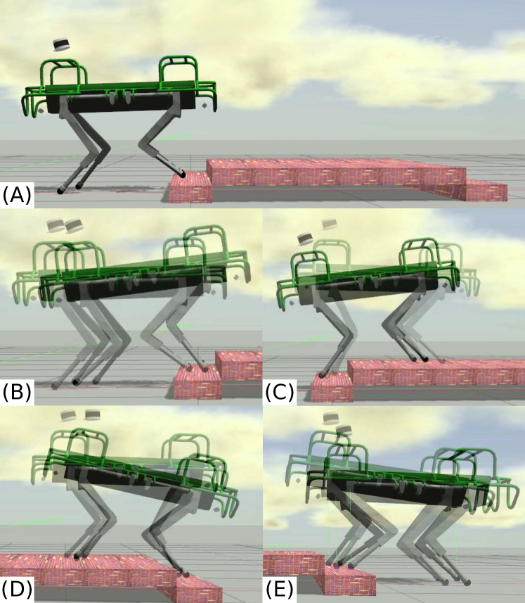
Figure 5.4: HyQ climbing stairs in simulation. (A) The full scenario. (B) The robot pitches up to allow for safe footholds for the front legs. (C) The robot lifts up the hind hips to avoid hind leg collisions with the step. (D) The robot pitches down to allow for safe footholds for the front legs. (E) The robot lowers the hind hips to allow for safe footholds for the legs when stepping down.

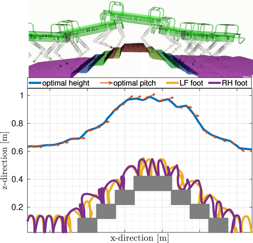
Figure 5.5: Climbing Stairs: A More Complex Scenario. Top: Overlayed screenshots of HyQ climbing stairs. Bottom: the optimal height and corresponding pitch (presented by the arrows) and the foot trajectories of LF and RH legs.

We carried out multiple simulations where HyQ is climbing the stairs shown in Fig. 5.4. Each step has a rise of 10 cm, and a go of 25 cm. HyQ is commanded to trot with a desired forward velocity of 0.2 m/s using the VPA and the VFA. Figure 5.4 shows screenshots of one simulation run, and Video 1 shows three simulation runs.

Figure 5.4 shows the ability of the VPA in adapting the robot pose to increase the chances of the legs to succeed in finding a safe foothold. In Fig. 5.4(B), HyQ raised its body and pitched upwards so that the front hips are raised to increase the workspace of the front legs when stepping up. In Fig. 5.4(C), HyQ raised its body and pitched downwards so that the hind hips are raised. This is done for two reasons. First, to have a larger clearance between the hind legs and the obstacle, and thus avoiding leg collision with the edge of the stairs. Second, to increase the workspace of the hind legs when stepping up, and thus avoiding reaching the workspace limits and collisions along the foot swing trajectory. In Fig. 5.4(D), HyQ lowered its body and pitched downwards so that the front hips are lowered. This is done for two reasons: First, to increase the workspace of the front legs when stepping down, and thus avoiding reaching the workspace limits. Second, to have a larger clearance between the front legs and the obstacle, and thus avoiding leg collisions. In Fig. 5.4(E), HyQ lowered its hind hips to increase the hind legs’ workspace when stepping down.

Throughout these simulations, the robot continuously adapted its body pose and its feet to find the best trade-off between increasing the kinematic feasibility, and avoiding trajectory and leg collision. This can be seen in Video 1 where the robot’s legs and the corresponding feet trajectories never collided with the terrain. The robot took multiple steps around the same foot location before stepping over an obstacle. The reason behind this is that the robot waited for the VPA to change the pose and allow for safe footholds, and then the VFA took the decision of stepping over the obstacle.

We carried out another scenario where HyQ is climbing the stairs setup in Fig. 5.5 where each step has a rise of 10 cm, and a go of 25 cm. HyQ is commanded to trot with a desired forward velocity of $0.2$m/s using ViTAL. The results are reported in Fig. 5.5 and Video 2. Figure 5.5 shows the robot’s height and pitch based on the VPA, and the corresponding feet trajectories of the LF leg and the RH leg based on the VFA. HyQ’s behavior was similar to the previous section: it accomplished the task without collisions or reaching workspace limits.

5.6.2   Climbing Stairs (Experiments)

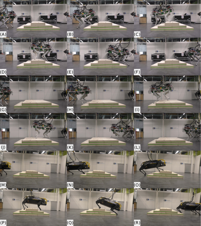
Figure 5.6: HyQ and HyQReal climbing stairs in experiment. (A-F) HyQ crawling over with 0.1 m/s commanded forward velocity. (G-L) HyQ trotting over with 0.25 m/s commanded forward velocity. (M-R) HyQReal crawling over with 0.2 m/s commanded forward velocity.

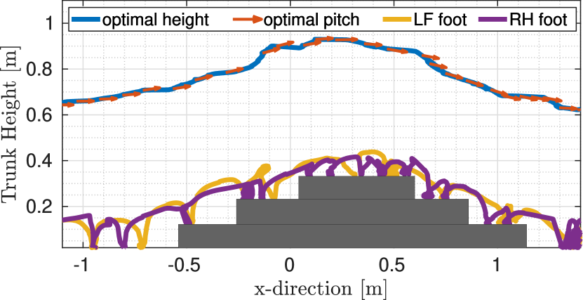
Figure 5.7: HyQ climbing stairs in experiment. The figure shows the optimal height and corresponding pitch (presented by the arrows) based on the VPA, and the foot trajectories of the LF and RH legs based on the VFA.

To validate ViTAL in experiments, we created three sets of experiments using the setups shown in Fig. 5.1. Each step has a rise of 10 cm, and a go of 28 cm.

In the first set of experiments, HyQ is commanded to crawl over the setups in Fig. 5.1(A,B) with a desired forward velocity of 0.1 m/s using the VPA and the VFA. Figures 5.6(A-F) show screenshots of one trial. Video 3 shows HyQ climbing back and forth the setup in Fig. 5.1(B) five times. Video 4 shows HyQ climbing the Fig. 5.1(A) setup, which is reported in Fig. 5.7. Figure 5.7 shows the robot’s height and pitch based on the VPA, and the corresponding feet trajectories of the Left-Front (LF) leg and the Right-Hind (RH) leg based on the VFA. This set of experiments confirms that ViTAL is effective on the real platform. The robot managed to accomplish the task without collisions or reaching workspace limits.

In the second set of experiments, HyQ is commanded to trot over the setup in Fig. 5.1(B) with a desired forward velocity of 0.25 m/s using the VPA and the VFA. Figures 5.6(G-L) show separate screenshots of this trial. Video 5 shows three trials of HyQ climbing the same setup. This set of experiments shows that ViTAL can handle different gaits.

Finally, in the third set of experiments, HyQReal is commanded to crawl over the setup in Fig. 5.1(C) with a desired forward velocity of 0.2 m/s using the VPA and the VFA. The results are reported in Fig. 5.6(M-R) that show screenshots of this trial. Video 6 shows HyQReal climbing this stair setup (Fig. 5.1(C)). This set of experiments shows that ViTAL can work on different legged platforms.

Table 5.1: Mean Absolute Tracking Errors of the Body Pitch $\beta$ and Height $z_{b}$ of HyQ & HyQReal using ViTAL in the Experiments detailed in Section 5.6.2 and in Fig. 5.1.

Description	$\beta$ [deg]	$z_{b}$ [cm]
Exp. (A): HyQ crawling at 0.1 m/s	1.0	1.5
Exp. (B): HyQ trotting at 0.2 m/s	1.0	2.3
Exp. (C): HyQReal crawling at 0.2 m/s	1.0	4.2

The tracking performance of these three sets of experiments are shown in Table 5.1. The table shows the mean absolute tracking errors of the body pitch $\beta$ and height $z_{b}$ of HyQ and HyQReal.

5.6.3   Climbing Stairs with Different Forward Velocities

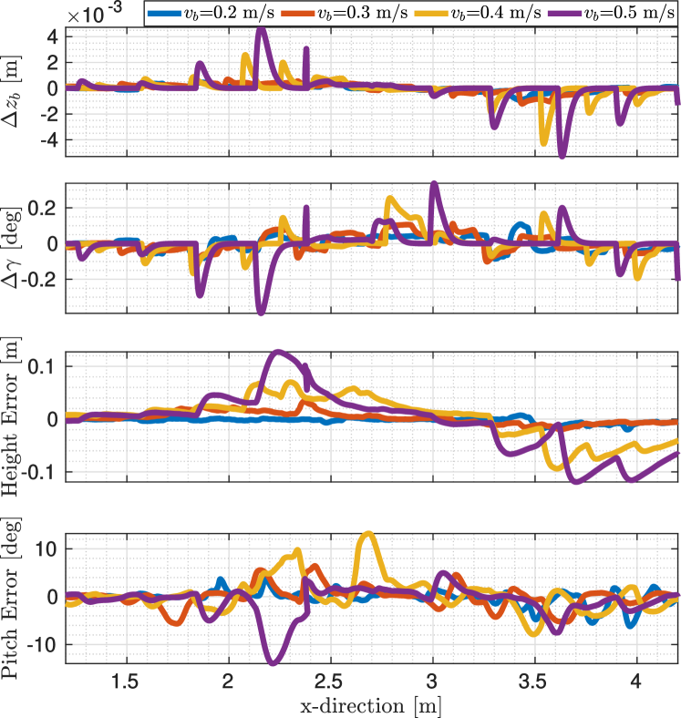
Figure 5.8: HyQ’s performance using ViTAL under different commanded velocities. The top two plots show the numerical difference of the body height and pitch ($\Delta z_{b}$ and $\Delta\gamma$), and the bottom two plots show the tracking errors of the body height and pitch.

Table 5.2: Mean Absolute Tracking Errors of the Body Pitch $\beta$ and Height $z_{b}$ of HyQ using ViTAL in Simulation with Different Forward Velocities as Detailed in Section 5.6.3 and Fig. 5.8.

Description	$\beta$ [deg]	$z_{b}$ [cm]
Sim. (A): HyQ trotting at 0.2 m/s	0.7	0.3
Sim. (B): HyQ trotting at 0.3 m/s	1.1	0.7
Sim. (C): HyQ trotting at 0.4 m/s	2.3	2.6
Sim. (D): HyQ trotting at 0.5 m/s	1.6	3.8

We evaluate the performance of HyQ under different commanded velocities using ViTAL. We carried out a series of simulations using the stairs setup shown in Fig. 5.5. HyQ is commanded to trot at four different forward velocities: 0.2 m/s, 0.3 m/s, 0.4 m/s, and 0.5 m/s. The results are reported in Fig. 5.8 and in Video 7. Additionally, the tracking performance of these series of simulations at the four different forward velocities are shown in Table 5.2. The table shows the mean absolute tracking errors of the body pitch $\beta$ and height $z_{b}$ of HyQ at the corresponding commanded forward velocity. Figure 5.8 shows the numerical differences $\Delta z_{b}$ and $\Delta\gamma$, and the tracking errors of the body height and pitch, respectively.

HyQ was able to climb the stairs terrain under different commanded velocities. However, as the commanded velocity increases, HyQ started having faster (abrupt) changes in the body pose as shown in the top two plots of Fig. 5.8. As a result, the height and pitch tracking errors increase proportionally to the commanded speed as shown in the bottom two plots of Fig. 5.8. This can also be seen in Table 5.2 where the mean absolute tracking errors of the pitch and height increase proportionally to the commanded speed.

Similarly to HyQ, we evaluate ViTAL on HyQReal and commanded it to trot with five different forward velocities: 0.2 m/s, 0.3 m/s, 0.4 m/s, 0.5 m/s, and 0.75 m/s. We report this simulation in Video 8 where we show that ViTAL is robot independent. Yet, since the workspace of HyQReal is larger than HyQ, this scenario was more feasible to traverse for HyQReal. Thus, HyQReal was able to reach a higher commanded velocity than the ones reported for HyQ.

5.6.4   Comparing the VPA with a Baseline (Experiments)

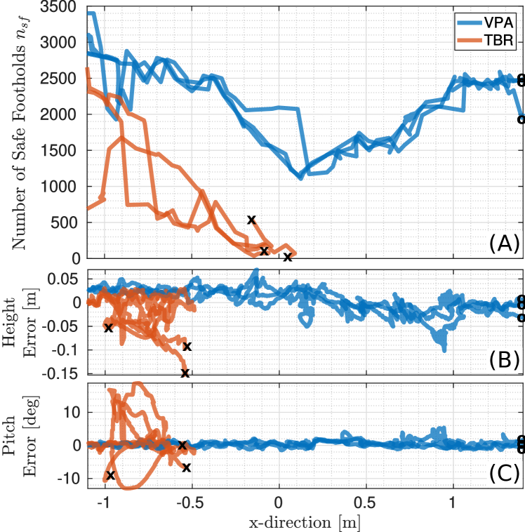
Figure 5.9: The difference between the VPA and the TBR in six experiments (3 each). (A) The number of safe footholds corresponding to the robot pose. (B,C) The body height and pitch tracking errors, respectively. Circles (o) and crosses (x) are successful and failed trials, respectively. Unlike the VPA, the TBR failed to climb the stairs because the TBR resulted in almost no safe footholds for the four legs to reach.

We compare the VPA with another vision-based pose adaptation strategy: the Terrain-Based Body Reference (TBR) [114]. The TBR generates pose references based on the footholds selected by the VFA. The TBR fits a plane that passes through the given selected footholds, and sets the orientation of this plane as a body orientation reference to the robot. The elevation reference of the TBR is a constant distance from the center of the approximated plane that passes through the selected footholds. We chose the TBR instead of an optimization-based strategy since the latter does not provide references that are fast enough with respect to the VPA.

Using the stairs setup in Fig. 5.1(A), we conducted six experimental trials: three with the VPA and three with the TBR. All trials were with the VFA. In all trials, HyQ is commanded to crawl with a desired forward velocity of 0.1 m/s. The results are reported in Fig. 5.9 and Video 9. Figure 5.9(A) shows the number of safe footholds corresponding to the robot pose from the VPA and the TBR. The robot height and pitch tracking errors are shown in Fig. 5.9(B,C), respectively.

As shown in Video 9, HyQ failed to climb the stairs with the TBR, while it succeeded with the VPA. This is because, unlike the VPA, the TBR does not aim to put the robot in a pose that maximizes the chances of the legs to succeed in finding safe footholds. As shown in Fig. 5.9(A), the number of safe footholds from using the TBR was below the ones from using the VPA. During critical periods when the robot was around 0 m in the x-direction, the number of safe footholds from using the TBR almost reached zero. The low number of safe footholds for the TBR compared to the VPA is reflected in the tracking of the robot height and pitch as shown in Fig. 5.9(B,C) where the tracking errors from the TBR were higher than the VPA.

The difference between the VPA and the TBR can be further explained in Video 9. When the TBR is used, the robot is adapting its pose given the selected foothold. But, if the selected foothold is not reached, or if there is a high tracking error, the robot reaches a body pose that results in a smaller number of safe footholds. Thus, the feet end up colliding with the terrain and hence the robot falls. On the other hand, the VPA is able to put the robot in a pose that maximizes the number of safe footholds. As a result, the feet found alternative safe footholds to select from, which resulted in no collision, and succeeded in climbing the stairs. The VPA optimizes for the number of safe footholds. Thus, if there is a variation around the optimal pose (tracking error), the VFA still finds more footholds to step on, which is not the case with the TBR.

5.6.5   Comparing the VPA with a Baseline (Simulation)

Similar to experiments, and using the stairs setup in Fig. 5.5, we compare the VPA with the TBR. We conducted six simulations: three with the VPA and three with the TBR. All trials were with the VFA. In all trials, HyQ is commanded to trot with a $0.2$m/s desired forward velocity. The results are reported in Fig. 5.10 and Video 10. Figure 5.10(A) shows the number of safe footholds corresponding to the robot pose from the VPA, and the TBR. The tracking errors of the robot height and pitch are shown in Fig. 5.10(B,C), respectively. These trials show that HyQ failed to climb the stairs using the TBR, while it succeeded using the VPA.

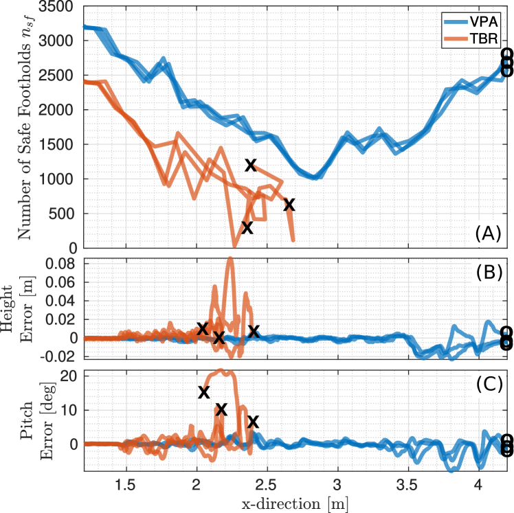
Figure 5.10: The difference between the VPA and the TBR in six simulations (3 each). (A) The number of safe footholds corresponding to the robot pose. (B,C) The body height and pitch tracking errors, respectively. Circles (o) and crosses (x) are successful and failed trials, respectively. Unlike the VPA, the TBR failed to climb the stairs because the TBR resulted in almost no safe footholds for the four legs to reach.

5.6.6   Climbing Stairs with Gaps

We show HyQ’s capabilities of climbing stairs with gaps using ViTAL, and we compare the VPA with the TBR. In this scenario, HyQ is commanded to trot at 0.4 m/s. Figure 5.11(A) shows overlayed screenshots of the simulation and the used setup. Figure 5.11(B) shows the robot’s height and pitch based on the VPA, and the corresponding feet trajectories of the LF leg and the RH leg based on the VFA, and Fig. 5.11(C) shows the number of safe footholds using the VPA and the TBR. Because of ViTAL, HyQ was able to climb the stairs with gaps while continuously adapting its pose and feet. Furthermore, the number of safe footholds from using the TBR is always lower than from using the VPA, which shows that indeed the VPA outperforms the TBR. Video 11 shows the output of this simulation using ViTAL.

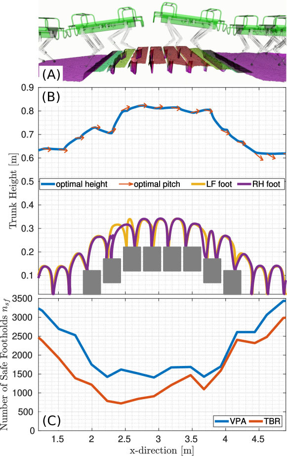
Figure 5.11: HyQ climbing gapped stairs. (A) Screenshots of HyQ climbing the setup. (B) The robot’s height and pitch based on the VPA, and the corresponding feet trajectories of the LF and RH legs based on the VFA. (C) The number of safe footholds using the VPA and the TBR.

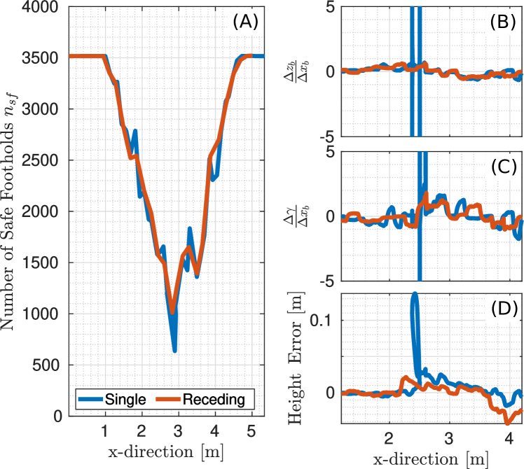
Figure 5.12: Pose Optimization: Single vs. Receding Horizons. (A) The number of safe footholds. (B) Variation (numerical difference) of the robot’s height. (C) Variation (numerical difference) of the robot’s pitch. (D) The tracking error of the robot’s height.

5.6.7   Pose Optimization: Single vs. Receding Horizons

To analyze the differences between the receding horizon and the single horizon in pose optimization, we use the stairs setup in Fig. 5.5 with a commanded forward velocity of 0.4 m/s, and report the outcome in Fig. 5.12 and Video 12. The main advantage of using a receding horizon instead of a single horizon is that the pose optimization can consider future decisions. Thus, if the robot is trotting at higher velocities, the pose optimizer can adapt the robot’s pose before hand. This can result in a better adaptation strategy with less variations in the generated optimal pose. Thus, we analyze the two approaches by taking a look at the variations in the body pose

$$\acute{z}_{b}=\frac{\Delta z_{b}}{\Delta x_{b}}~{},~{}~{}~{}\text{and}~{}~{}~{}\acute{\gamma}=\frac{\Delta\gamma}{\Delta x_{b}}$$ (5.26)

where $\acute{z}_{b}$ and $\acute{\gamma}$ are the numerical differences (variations) of the robot height $z_{b}$ and pitch $\gamma$ with respect to the robot forward position $x_{b}$, respectively.

Figure 5.12 reports the differences between the two cases. The number of safe footholds is shown in Fig. 5.12(A). The variations in $\acute{z}_{b}$ and $\acute{\gamma}$ are shown in Fig. 5.12(B,C), respectively. Finally, the tracking error of the robot’s height is shown in Fig. 5.12(D). As shown in Figure 5.12 the receding horizon resulted in less variations in the body pose compared to the single horizon. This resulted in a smaller tracking error for the receding horizon in the body height, which resulted in slightly larger number of safe footholds. All in all, the receding horizon reduces variations in the desired trajectories which improves the trajectory tracking response.

The differences between the receding and single horizon in the pose optimization can also be noticed in Video 12. In the case of a single horizon, the robot was struggling while climbing up the stairs but was able to recover and accomplish the task. However, using the receding horizon, the robot was able to adapt its pose in time, and thus resulting in safer footholds that allowed the robot to accomplish the task.

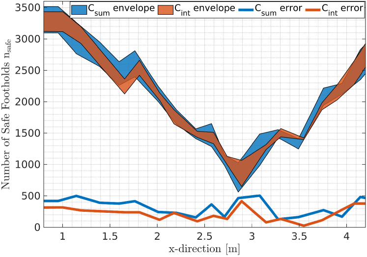
Figure 5.13: Pose Optimization: $\mathcal{C}_{\mathrm{sum}}$ vs. $\mathcal{C}_{\mathrm{int}}$. The shaded areas are the envelopes of the number of safe footholds. The lines are the thicknesses (errors) between these envelopes.

5.6.8   Pose Optimization: $\mathcal{C}_{\mathrm{sum}}$ vs. $\mathcal{C}_{\mathrm{int}}$

To analyze the differences between $\mathcal{C}_{\mathrm{sum}}$ and $\mathcal{C}_{\mathrm{int}}$ in the pose optimization, we use the stairs setup in Fig. 5.5 with a commanded forward velocity of 0.4 m/s, and report the outcome in Fig. 5.13. The main advantage of using $\mathcal{C}_{\mathrm{int}}$ over $\mathcal{C}_{\mathrm{sum}}$ is that $\mathcal{C}_{\mathrm{int}}$ will result in a pose that does not just maximize the number of safe footholds for all of the legs, but also ensures that the number of safe footholds of the poses around the optimal pose is still high. To compare the two cost functions, we take a look at the number of safe footholds. In particular, we evaluate the number of safe footholds corresponding to the optimal pose, and the poses around it with a margin of $m=$ 0.025 m. Thus, in Fig. 5.13, we plot the envelope (shaded area) between $\hat{\mathcal{F}}(u^{*}+m)$ and $\hat{\mathcal{F}}(u^{*}-m)$ for both cases, and the thickness between these envelopes which we refer to as error

$$\textbf{error}~{}=|\hat{\mathcal{F}}(u^{*}+m)-\hat{\mathcal{F}}(u^{*}-m)|.$$ (5.27)

As shown in Fig. 5.13 the envelope of the number of safe footholds resulting from $\mathcal{C}_{\mathrm{int}}$ is almost always encapsulated by $\mathcal{C}_{\mathrm{sum}}$. The thickness (error) of the number of safe footholds resulting from using $\mathcal{C}_{\mathrm{int}}$ is always smaller than $\mathcal{C}_{\mathrm{sum}}$. This means that any variation of $m$ in the optimal pose will be less critical if $\mathcal{C}_{\mathrm{int}}$ is used compared to $\mathcal{C}_{\mathrm{sum}}$.

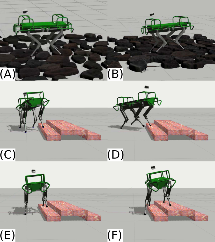
Figure 5.14: HyQ traversing rough terrain and climbing stairs sideways. (A,B) HyQ traversing rough terrain with and without ViTAL, respectively. (C,D) HyQ climbing stairs while yawing (commanding the yaw rate) using ViTAL. (E,F) HyQ climbing stairs sideways using ViTAL.

5.6.9   Locomotion over Rough Terrain

We evaluate the performance of HyQ in traversing rough terrain as shown in Fig. 5.14(A,B) and in Video 13. We conducted two simulations: one with ViTAL and thus with exteroceptive and proprioceptive reactions as shown in Fig. 5.14(A), and another without ViTAL and thus only with proprioceptive reactions as shown in Fig. 5.14(B). HyQ was commanded to traverse the rough terrain with a forward velocity of 0.2 m/s. No hyper parameters re-tuning, or CNNs re-training were needed.

As shown in Video 13, HyQ was able to successfully traverse the terrain in both cases. With ViTAL, HyQ collided less with the terrain and continuously adapted its footholds over the small cobblestones. Without ViTAL, HyQ traversed the rough terrain, yet, with significantly more effort. Additionally, without ViTAL, HyQ continuously collided with the terrain, and in some incidents, the feet got stuck. For this reason, we had to re-tune the gait parameters, and increase the step height to reduce these incidents. The robot’s feet also kept slipping since the feet were always close to edges and corners.

5.6.10   Climbing Stairs with Different Commands

Instead of commanding only forward velocities as in the previous sections, we command HyQ to climb the stairs with ViTAL while yawing (commanding the yaw rate) as shown in Video 14 and Fig. 5.14(C,D), and to climb stairs laterally as shown in Video 15 and Fig. 5.14(E,F). Climbing stairs sideways is more challenging than facing the stairs since the range of motion of the robot’s roll orientation is more restricted versus the pitch orientation. That said, because of ViTAL, HyQ was still able to climb these stairs in both cases as shown in Video 14 and Video 15.

5.7  Conclusion

We presented ViTAL which is an online vision-based locomotion planning strategy. ViTAL consists of the VPA for pose adaptation, and the VFA for foothold selection. The VPA introduces a different paradigm to current state-of-the-art pose adaptation strategies. The VPA finds body poses that maximize the chances of the legs to succeed in reaching safe footholds. This notion of success emerges from the robot’s skills. These skills are encapsulated in the FEC that include (but are not limited to) the terrain roughness, kinematic feasibility, leg collision, and foot trajectory collision. The VFA is a foothold selection algorithm that continuously adapts the robot’s trajectory based on the FEC. The VFA algorithm of this work extends our previous work in [121, 114] as well as the state of the art [113, 118]. Since the computation of the FEC is usually expensive, we rely on approximating these criteria with CNNs.

The robot’s skills and the notion of success provided by the FEC allowed the VPA to generate body poses that maximize the chances of success in reaching safe footholds. This resulted in body poses that are aware of the terrain and aware of what the robot and its legs can do. For that reason, the VPA was able to generate body poses that give a better chance for the VFA to select safe footholds. As a result, because of ViTAL, HyQ and HyQReal were able to traverse multiple terrains with various forward velocities and different gaits without colliding or reaching workspace limits. The terrains included stairs, gaps, and rough terrains, and the commanded velocities varied from 0.2 m/s to 0.75 m/s. The VPA outperformed other strategies for pose adaptation. We compared VPA with the TBR which is another vision based pose adaptation strategy, and showed that indeed the VPA puts the robot in a pose that provides the feet with higher number of safe footholds. Because of this, the VPA made our robots succeed in various scenarios where the TBR failed.

5.8  Limitations and Future Work

One issue that we faced during experiment was in tracking the motion of the robot, especially for HyQReal. We were using a WBC for motion tracking. We believe that the motion tracking and our strategy can be improved by using a Model Predictive Control (MPC) alongside the WBC. Similarly, instead of using a model-based controller (MPC or WBC), we hypothesize that an RL-based controller can also improve the robustness and reliability of the overall robot behavior.

As explained in Section 5.5, one other key limitation was regarding the perception system. State estimation introduced a significant drift that caused a major noise and drift in the terrain map. Albeit not being a limitation to the suggested approach, we plan on improving the state estimation and perception system of HyQ and HyQReal to allow us to test ViTAL in the wild.

The pose optimization problem of the VPA does not reason about the robot’s dynamics. This did not prevent HyQ and HyQReal from achieving dynamic locomotion while traversing challenging terrains at high speeds. However, we believe that incorporating the robot’s dynamics into ViTAL may result in a better overall performance. That said, we believe that in the future, the VPA should also reason about the robot’s dynamics. For instance, one can augment the FEC with another criterion that ensures that the selected footholds are dynamically feasible by the robot.

Additionally, in the future, we plan to extend the VPA of ViTAL to not only send pose references, but also reason about the robot’s body twist. We also plan to augment the robot skills to not only consider foothold evaluation criteria, but also skills that are tailored to the robot pose. Finally, in this work, ViTAL considered heightmaps which are 2.5D maps. In the future, we plan to consider full 3D maps that will enable ViTAL to reason about navigating in confined space (inspired by [115]).

Chapter 6  ViTAL - Implementation Details

6.1  CNN approximation in the VFA and the VPA

In the VFA, the foothold evaluation stage is approximated with a CNN [133] as explained in Remark 5.3. The CNN approximates the mapping between $T_{\mathrm{vfa}}$ and $p_{*}$. The heightmap $H_{\mathrm{vfa}}$ in $T_{\mathrm{vfa}}$ passes through three convolutional layers with $5\times 5$ kernels, $2\times 2$ padding, Leaky ReLU activation [134], and $2\times 2$ max-pooling operation. The resulted one-dimensional feature vector is concatenated with the rest of the variables in the tuple $T_{\mathrm{vfa}}$, namely, $z_{h},v_{b},\alpha,$ and $p_{n}$. This new vector passes through two fully-connected layers with Leaky ReLU and softmax activations. The parameters of the CNN are optimized to minimize the cross-entropy loss [135] of classifying a candidate foothold location as optimal $p_{*}$.

In the VPA, the pose evaluation and the function approximation is approximated with a CNN as explained in Remark 5.5. The CNN infers the weights $w$ of $\hat{\mathcal{F}}$ given $T_{\mathrm{vpa}}$ (the mapping between $T_{\mathrm{vpa}}$ and $w$). The heightmap $H_{\mathrm{vpa}}\in\mathbb{R}^{33\times 33}$ passes through three convolutional layers with $5\times 5$ kernels, $2\times 2$ padding, Leaky ReLU activation, and $2\times 2$ max-pooling operation. The body velocities $v_{b}$ pass through a fully-connected layer with Leaky ReLU activation that is then concatenated with the one-dimensional feature vector obtained from the heightmap. This new vector passes through two fully-connected layers with Leaky ReLU and linear activations. The parameters of this CNN are optimized to minimize the mean squared error loss between the number of safe footholds $\mathrm{n_{sf}}$ predicted by $\hat{\mathcal{F}}(z_{h},w)$ and $\hat{\mathcal{F}}(z_{h},\hat{w})$ where $\hat{w}$ are the function parameters approximated by the CNN.

For both CNNs, we used the Adam optimizer [136] with a learning rate of $0.001$, and we used a validation-based early-stopping using a $9$-to-$1$ proportion to reduce overfitting. The datasets required for training this CNNs are collected by running simulated terrain scenarios that consist of bars, gaps, stairs, and rocks. In this work, we considered a $33\times 33$ heightmap with a resolution of 0.02 m ($H_{\mathrm{vfa}},H_{\mathrm{vpa}}\in\mathbb{R}^{33\times 33}$).

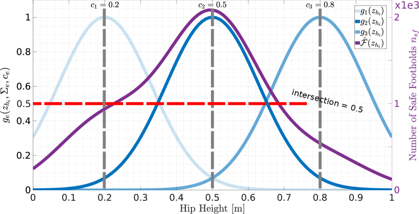
Figure 6.1: An illustration of the Function Approximation of the VPA.

6.2  On the Function Approximation of the VPA

As explained in Section 5.4.4, the function $\hat{\mathcal{F}}(z_{h_{i}},w)$

$$\hat{\mathcal{F}}(z_{h_{i}},w)=\sum_{e=1}^{E}w_{e}\cdot g(z_{h_{i}},\Sigma_{e},c_{e})$$ (6.1)

is defined as the weighted sum of Gaussian basis functions

$$g(z_{h_{i}},\Sigma_{e},c_{e})=\text{exp}(-0.5(z_{h_{i}}-c_{e})^{T}\Sigma_{e}^{-1}(z_{h_{i}}-c_{e})).$$ (6.2)

The parameters $\Sigma_{e}$ and $c_{e}$ are the widths and centers of the Gaussian function $g_{e}$ (see Section 3.1 in [65]). In the literature, $c_{e}$ is usually referred to as the mean or the expected value, and $\Sigma_{e}$ as the standard deviation. The regression algorithm should predict the weights $w_{e}$, and the parameters $\Sigma_{e}$ and $c_{e}$. To reduce the dimensionality of the problem, as explained in Section 5.4.4, and in Section 4.1 in [65], we decided to fix the values of the parameters of the Gaussian functions $\Sigma_{e}$ and $c_{e}$. In detail, the centers $c_{e}$ are spaced equidistantly within the bounds of the hip heights $z_{h_{i}}$, and the widths are determined by the value at which the Gaussian functions intersect. That way, the regression algorithm only outputs the weights $w_{e}$. Figure 6.1 shows an example of the function approximation. In this example, the bounds of the hip heights $z_{h_{i}}$ are 0.2 m and 0.8 m. Assuming a number of basis functions $E=3$, the centers $c_{e}$ are then chosen to be equidistant within the bounds, and thus, the centers $c_{e}$ are 0.2 m, 0.3 m and 0.8 m. By choosing the Gaussian functions to intersect at 0.5, the widths $\Sigma_{e}$ are 0.13.

6.3  Representing the Hip Heights in terms of the Body Pose

To represent the hip heights in terms of the body pose, we first write the forward kinematics of the robot’s hips

$$p_{h_{i}}^{W}=p_{b}^{W}~{}+~{}R_{b}^{W}p_{h_{i}}^{b}$$ (6.3)

where $p_{h_{i}}^{W}\in\mathbb{R}^{3}$ is the position of the hip of the $i$th leg in the world frame, $p_{b}^{W}\in\mathbb{R}^{3}$ is the position of the robot’s base in the world frame, $R_{b}^{W}\in SO(3)$ is the rotation matrix mapping vectors from the base frame to the world frame, and $p_{h_{i}}^{b}\in\mathbb{R}^{3}$ is the position of the hip of the $i$th leg in the base frame. The rotation matrix $R_{b}^{W}$ is a representation of the Euler angles of the robot’s base with sequence of roll $\beta$, pitch $\gamma$, and yaw $\psi$ (Cardan angles) [137]. The variable $p_{h_{i}}^{b}$ is obtained from the CAD of the robot. Expanding (6.3) yields

$$\begin{bmatrix}x_{h_{i}}^{W}\\ y_{h_{i}}^{W}\\ z_{h_{i}}^{W}\end{bmatrix} = \begin{bmatrix}x_{b}^{W}\\ y_{b}^{W}\\ z_{b}^{W}\end{bmatrix}+R_{b}^{w}(\beta,\gamma,\psi)\begin{bmatrix}x_{h_{i}}^{b}\\ y_{h_{i}}^{b}\\ z_{h_{i}}^{b}\end{bmatrix}$$ (6.4)

$$= \begin{bmatrix}x_{b}^{W}\\ y_{b}^{W}\\ z_{b}^{W}\end{bmatrix}+\begin{bmatrix}\cdots&\cdots&\cdots\\ \cdots&\cdots&\cdots\\ -s\gamma&c\gamma~{}s\beta&c\gamma~{}c\beta\end{bmatrix}\begin{bmatrix}x_{h_{i}}^{b}\\ y_{h_{i}}^{b}\\ z_{h_{i}}^{b}\end{bmatrix}$$ (6.5)

where $s$ and $c$ are sine and cosine of the angles, respectively. Since we are interested only in the hip heights, the z-component (third row) of (6.5) yields

$$z_{h_{i}}^{W}=z_{b}^{W}-x_{h_{i}}^{b}s\gamma+y_{h_{i}}^{b}c\gamma s\beta+z_{h_{i}}^{b}c\gamma c\beta.$$ (6.6)

6.4  Using the Sum of Squared Integrals in the Pose Optimization of the VPA

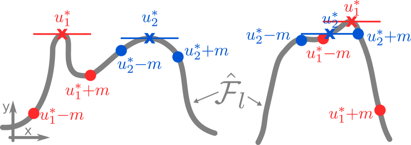
Figure 6.2: Using the sum of squared integrals as a cost function in the pose optimization of the VPA. The two curves represent $\hat{\mathcal{F}}_{l}$. The x-axis is the hip height and the y-axis is $\mathrm{n_{sf}}$. The figure shows two optimal poses: $u_{1}^{*}$ which is from using $\mathcal{C}_{\mathrm{sum}}$ or $\mathcal{C}_{\mathrm{prod}}$, and $u_{2}^{*}$ which is from using $\mathcal{C}_{\mathrm{int}}$.

Using $\mathcal{C}_{\mathrm{int}}$ as a cost function can be motivated by taking Fig. 6.2 as an example. In this figure, there are two curves that represent $\hat{\mathcal{F}}_{l}$ where the horizontal axis is the hip height and the vertical axis represent $\mathrm{n_{sf}}$. The figure shows two optimal poses where $u_{1}^{*}$ is the optimal pose using the cost functions $\mathcal{C}_{\mathrm{sum}}$ or $\mathcal{C}_{\mathrm{prod}}$ that only maximize for $\hat{\mathcal{F}}_{l}$, and $u_{2}^{*}$ is the optimal pose using the cost function $\mathcal{C}_{\mathrm{int}}$. As shown in the figure, if $\mathcal{C}_{\mathrm{sum}}$ or $\mathcal{C}_{\mathrm{prod}}$ is used, the optimal pose will be $u_{1}^{*}$ which is indeed the one that results in the maximum $\hat{\mathcal{F}}_{l}$. However, if there is a tracking error of $m$ (thus the robot reaches $u_{1}^{*}\pm m$), the robot might end up in the pose $u_{1}^{*}\pm m$ that results in a small number of safe footholds. Using $\mathcal{C}_{\mathrm{int}}$ will take into account the safe footholds within a margin $m$. This might result in a pose that does not yield the maximum number of safe footholds, but it will result in a safer foothold in case the robot pose has any tracking errors. Note that using the sum of squared integrals $\mathcal{C}_{\mathrm{int}}$ as a cost function is similar to smoothing $\hat{\mathcal{F}}_{l}$ with respect to the hip height (a moving average smoothing). Using a smoothing function $\mathcal{C}_{s}$ may take the form

$$\mathcal{C}_{s}=\sum_{l=1}^{N_{l}=4}\|\frac{1}{2\epsilon}\sum_{i=-\epsilon}^{\epsilon}\hat{\mathcal{F}}_{l}(z_{h_{l}}+i)\ \|^{2}_{Q}.$$ (6.7)

6.5  Defining the Receding Horizon

In the receding horizon there is a tuple $T_{\mathrm{vpa},j}$ for every $j$th horizon that is defined as

$$T_{\mathrm{vpa},j}=(H_{\mathrm{vpa},j},v_{b},\alpha)$$ (6.8)

hence sharing the same body twist $v_{b}$ and gait parameters $\alpha$ but a different heightmap $H_{\mathrm{vpa},j}$. For every leg, a heightmap of horizon $j+1$ is overlapping with the previous horizon’s $j$ heightmap. This overlap has a magnitude of $\Delta h$ taking the same direction as the body velocity $\dot{x}_{b}$. Without loss of generality, we chose the magnitude of the overlap to be half of the diagonal size of the heightmap in this work. To sum up, we first gather $T_{\mathrm{vpa},j}$ that share the same $v_{b}$ and $\alpha$, but a different $H_{\mathrm{vpa},j}$. Then, we evaluate $T_{\mathrm{vpa},j}$ and approximate the output using the function approximation yielding $\hat{\mathcal{F}}_{j}$ that is sent to the optimizer for all of the legs.

6.6  Miscellaneous Settings

In this work, all simulations were conducted on an Intel Core i7 quad-core CPU, and all experiments were running on an onboard Intel Core i7 quad-core CPU where state estimation, mapping, and controls were running. The RCF (including the WBC) runs at 250 Hz, the low-level controller runs at 1000 Hz, the state estimator runs at 333 Hz, and the mapping algorithm runs at 20 Hz. The VPA and the VFA run asynchronously at the maximum possible update rate.

ViTAL is implemented in Python. The CNNs are implemented in PyTorch [138]. As explained in Section 6.1, in this work, we considered a $33\times 33$ heightmap with a resolution of 0.02 m ($H_{\mathrm{vfa}},H_{\mathrm{vpa}}\in\mathbb{R}^{33\times 33}$). The finite set $\bar{\mathcal{Z}}$ consisted of a hip height range between 0.2 m and 0.8 m with a resolution of 0.02 m yielding $N_{z_{h}}=31$ samples. The number of radial basis functions used in the function approximation was $E=30$. The pose optimization problem is solved with a trust-region interior point method [139, 140] which is a non-linear optimization problem solver that we solved using SciPy [141]. The bounds of the pose optimization problem $u_{\min}$ and $u_{\max}$ are $[0.2\,\mathrm{m},-0.35\,\mathrm{rad},-0.35\,\mathrm{rad}]$, and $[0.8\,\mathrm{m},0.35\,\mathrm{rad},0.35\,\mathrm{rad}]$, respectively. We used a receding horizon of $N_{h}=2$ with a map overlap of half the size of the heightmap. For a heightmap of a size of $33\times 33$ and a resolution of 0.02 m, the map overlap $\Delta h$ is 0.33 m. We used Gazebo [142] for the simulations, and ROS for communication.

6.7  Estimation Accuracy

We compare the estimation accuracy of the VFA by comparing the output of the foothold evaluation stage (explained in Section 5.3) given the same input tuple $T_{\mathrm{vfa}}$. That is to say, we compare the estimation accuracy of the VFA by comparing $\hat{g}(T_{\mathrm{vfa}})$ versus $g(T_{\mathrm{vfa}})$ (see Remark 5.3). To do so, once trained, we generated a dataset of 4401 samples from randomly sampled heightmaps for every leg. This analysis was done on HyQ.

As explained in Section 5.3, from all of the safe candidate footholds in $\mu_{\mathrm{safe}}$, the VFA chooses the optimal foothold to be the one closest to the nominal foothold. Thus, to fairly analyse the estimation accuracy of the VFA, we present three main measures: perfect match being the amount of samples where $\hat{g}(T_{\mathrm{vfa}})$ outputted the exact value of $g(T_{\mathrm{vfa}})$, safe footholds, being the amount of samples where $\hat{g}(T_{\mathrm{vfa}})$ did not output the exact value of $g(T_{\mathrm{vfa}})$, but rather a foothold that is safe but not closest to the nominal foothold, and mean distance, being the average distance of the estimated optimal foothold from $\hat{g}(T_{\mathrm{vfa}})$ relative to the exact foothold from $g(T_{\mathrm{vfa}})$. These measures are presented as the mean of all legs.

Based on that, the perfect match measure is $74.0\%$. Thus, $74\%$ of $\hat{g}(T_{\mathrm{vfa}})$ perfectly matched $g(T_{\mathrm{vfa}})$. The safe footholds measure is $93.7\%$. Thus, $93.7\%$ of $\hat{g}(T_{\mathrm{vfa}})$ were deemed safe. Finally, the mean distance of the estimated optimal foothold from $\hat{g}(T_{\mathrm{vfa}})$ relative to the exact foothold from $g(T_{\mathrm{vfa}})$ is 0.02 m. This means that, on average, $\hat{g}(T_{\mathrm{vfa}})$ yielded optimal footholds that are 0.02 m far from the optimal foothold from $g(T_{\mathrm{vfa}})$. Note that, the radius of HyQ’s foot, and the resolution of the heightmap is also 0.02 m, which means that the average distance measure is still acceptable especially since we account for this value in the uncertainty margin as explained in Remark 5.1.

Similar to the VFA, we compare the accuracy of VPA by comparing the output of the pose evaluation stage (explained in Section 5.4.3) given the same input tuple $T_{\mathrm{vfa}}$. That is to say, we compare the estimation accuracy of the VPA by comparing $\bar{\mathcal{F}}$ versus $\hat{\mathcal{F}}$ (see Remark 5.4 and Remark 5.5). To do so, we ran one simulation using the stairs setup shown in Fig. 5.5 on HyQ, and gathered the input tuple $T_{\mathrm{vfa}}$. Then, we ran the VPA offline, once with the exact evaluation (yielding $\bar{\mathcal{F}}$) and once with the approximate one (yielding $\hat{\mathcal{F}}$).

Based on this simulation run, the mean values of the exact and the approximate evaluations are $\mathrm{mean}(\bar{\mathcal{F}})=1370$ and $\mathrm{mean}(\hat{\mathcal{F}})=1322$, respectively. This yields an estimation accuracy $\mathrm{mean}(\hat{\mathcal{F}})/\mathrm{mean}(\bar{\mathcal{F}})$ of $96.5\%$.

6.8  Computational Analysis

To analyze the computational time of the VFA and the VPA, we ran one simulation using the stairs setup shown in Fig. 5.5 on HyQ to gather the input tuples of the VFA and the VPA, $T_{\mathrm{vfa}}$ and $T_{\mathrm{vpa}}$, respectively. Then, we ran both algorithms offline, once with the exact evaluation and once using the CNNs, and collected the time it took to run both algorithms (all stages included). The mean and standard deviation of the time taken to compute the exact and the CNN-approximated VFA (per leg) algorithms are $7.5\,\mathrm{ms}\pm 1\,\mathrm{ms}$, and $3.5\,\mathrm{ms}\pm 1\,\mathrm{ms}$, respectively. The mean and standard deviation of the time taken to compute the exact and the CNN-approximated VPA algorithms are $720\,\mathrm{ms}\pm 68\,\mathrm{ms}$, and $180\,\mathrm{ms}\pm 60\,\mathrm{ms}$, respectively. Hence, the VFA and the VPA can run at roughly 280 Hz and 5 Hz, respectively. This also shows that the CNNs can speed up the evaluation of the VFA and the VPA up to 4 times and 2 times, respectively.

Note that it takes longer to compute the VFA of this work versus our previous work [114]. This is because the VFA of this work considers more inputs than in our previous work, and thus, the size of the CNN is larger. As can be seen, the VPA runs at a relatively lower update rate compared to the VFA. We believe that this is not an issue since the VFA runs at the legs-level while the VPA runs as the body-level which means that the legs experience faster dynamics than the body.

During simulations and experiments, the CNNs were running on a CPU. A significant amount of computational time can be reduced if we run the CNNs of the VFA and the VPA on a GPU. Likewise, a significant amount of computational time can be reduced if a different pose optimization solver is used. However, both suggestions are beyond the scope of this work, and are left as a future work.

Chapter 7  Conclusion

7.1  Summary

Terrain-Aware Locomotion (TAL) is an essential element to achieve Athletic Intelligence (AtI) for legged robots. For that to happen, legged robots should be able to perceive, understand, and adapt to their surrounding terrain using their proprioceptive and exteroceptive (visual) information. This thesis presented TAL strategies, both at the proprioceptive and vision-based level. The first part (Chapters 2-4) was on Proprioceptive Terrain-Aware Locomotion (PTAL) strategies and the second part (Chapter 5) was on Exteroceptive Terrain-Aware Locomotion (ETAL) strategies.

In Chapter 2, we presented a PTAL strategy that made legged robots adapt to the terrain inclination and frictional properties. We presented a Passive Whole-Body Control (pWBC) framework for quadruped robots where the locomotion control problem was casted as a Quadratic Program (QP) that took into account the full robot rigid body dynamics, the actuation limits, the joint kinematic limits and the contact interaction. The contact interaction included the terrain’s inclination (normals), frictional and unilaterality properties, and the rigid contact interaction, and were encoded in the QP formulation. We encoded the terrain inclination, frictional properties, and the rigid contact interaction in the QP formulation. As a result, the quadruped robot was able to reliably traverse various challenging terrains with different friction coefficients, and under different gaits.

In Chapter 3, we presented a PTAL strategy that made legged robots adapt to soft terrain. We introduced the Soft Terrain Adaptation aNd Compliance Estimation (STANCE) approach that extended capabilities of the previously presented pWBC in Chapter 2. STANCE consisted of a Compliant Contact Consistent Whole-Body Control (c³WBC) and a Terrain Compliance Estimator (TCE). The TCE provided the c³WBC with the current terrain impedance that the c³WBC then used to adapt the robot’s motion accordingly. As a result, the quadruped robot was able to differentiate between compliances under each foot, and to adapt online to multiple terrains with different compliances (rigid and soft) without pre-tuning.

In Chapter 4, we looked into one of the remaining limitations of locomotion over soft terrain. We were able to investigate how and why does soft terrain affect state estimation for legged robots. As a result, we showed that soft terrain negatively affects state estimation for legged robots, and that the state estimates have a noticeable drift over soft terrain compared to rigid terrain.

In Chapter 5, we presented a Vision-Based Terrain-Aware Locomotion (ViTAL) strategy consisting of a Vision-Based Pose Adaptation (VPA) algorithm that introduced a paradigm shift for pose adaptation strategies, and a Vision-Based Foothold Adaptation (VFA) algorithm that extended state-of-the-art foothold selection strategies. Instead of the commonly used pose adaptation techniques that optimizes body poses given the selected footholds, we proposed to find body poses that maximizes the chances of reaching safe footholds. This was done by relying on a set of robots skills that represented the capabilities of the robot and its legs. The skills were then learned via self-supervised learning using Convolutional Neural Networks (CNNs). ViTAL allowed our robots to select the footholds based on their capabilities, and simultaneously find poses that maximize the chances of reaching safe footholds. As a result, our quadruped robots were able to traverse stairs, gaps, and various other terrains at different speeds.

We believe that the contributions of this thesis allows legged robots to traverse a wider range of terrains with different geometries and physical properties. We believe that this would not have been possible without exploiting the robot’s proprioceptive and exteroceptive (visual) information.

7.2  Future Directions

The contributions of this thesis allowed us to advance in many research directions, yet, there remains many further improvements in these research directions. Below, we provide pointers to where we believe these improvements should be going.

Whole-Body Control

• Whole-Body Control (WBC) is still an active topic in research. Perhaps one promising direction is the use of control Lyapunov function based QP. This approach has shown a rapid convergence compared to the standard WBC formulations [143]. Yet, further validation of the approach should be done to show its capabilities in more challenging terrains and different gaits.

• WBC s are model-based optimization approaches that rely on inverse dynamics. Hence, one possible direction is to improve the robot dynamics model using model learning techniques. The hybrid nature of floating based systems makes it harder to learn its inverse dynamics. One approach is to learn the errors between the dynamics model and the actual dynamics (the residual in the dynamics) of the legged robot [144].

• There are other challenges in WBC in specific scenarios. One challenge is when the robot loses contact or if the robot gets lifted up. The current WBC formulations cannot handle this case. Thus, some implementations still rely on a joint-level PD loop albeit not being used in our work. Perhaps one way to improve this is to add constraints regarding the stance feet. These constraints would keep the stance feet close to the robot base, thus, if the robot gets lifted, the feet do not move away from the base.

Soft Terrain Adaptation

• As mentioned in Chapter 3, there are various research directions in locomotion over soft terrain mainly in state estimation and low-level control. The former was tackled in Chapter 4 while the latter is not yet tackled. With this in mind, we believe there is great potential improvements of low-level control to generalize beyond rigid terrain. As a first step, perhaps there should be a formal discussion on the effects of soft terrain on the low-level control, and possible ideas on how to improve the performance of the low-level control to adapt to terrains with different impedances.

• The c³WBC presented in Chapter 3 was superior to the Standard Whole-Body Control (sWBC). As we mentioned in Chapter 3, the differences between these two controllers were more evident under dynamic motions. Perhaps other WBCs could perform better than the sWBC and the c³WBC under slower motions. Hence, it might be of great potential to compare the c³WBC with the controllers mentioned in [145].

• The TCE presented in Chapter 3 relied on the Kelvin-Voigt’s (KV) model which is linear springs and dampers parallel and perpendicular to the contact point. As we reported in Chapter 3, we chose this model because it was simple, and it is computationally inexpensive. Based on that, we believe there is a lot of work to do in that aspect. First, it is perhaps important to analyze the trade-off between using a more complicated model (non-linear) that is slower to estimate its parameters versus a simpler model that is faster to compute.

• STANCE is implemented at the WBC level which resulted in the controller being compliant contact consistent (c³). One possible extension is to exploit the work of STANCE to also make Model Predictive Control (MPC) c³. For that, the MPC optimization problem should be re-formulated to take into account the terrain impedance parameters.

State Estimation

Although this thesis was not fundamentally focusing on state estimation, we believe that state estimation is crucial in TAL. TAL mandates an accurate estimate of the robot states as well as the map of the environment (terrain).

As we mentioned in Chapter 4, the performance of state estimation degrades on soft terrain. This is because state estimators still rely on rigid body assumptions mainly in leg odometry. One way to deal with that is to have a velocity bias in leg odometry. This velocity bias should be adaptive and not constant since it depends on the type of terrain and on the gait used. Perhaps another way to deal with this is to reformulate the leg odometry module and augment it with the terrain impedance knowledge.

Vision-based Terrain Aware Locomotion

We believe that our work on ViTAL and specifically the VPA algorithm introduced a different way of thinking and of approaching pose adaptation problems. This opened more research questions and a lot of possible improvements. ViTAL’s core idea is to teach the robot a set of skills. These skills were encapsulated by the Foothold Evaluation Criteria (FEC). Perhaps the most important future work in that aspect is to augment the robot with skills that are tailored to the robot’s pose and not just the legs. For example, the skills can include the robot’s ability to traverse confined spaces (inspired from [115]). Furthermore, in Chapter 5, we reported that we faced some issues during experiment. These issues were mainly in tracking the motion of the robot especially for HyQReal. Thus, a possible way to improve this is to use the MPC controller in [125].

Curriculum Vitae

Shamel Fahmi

www.shamelfahmi.com

Shamel Fahmi (S’19) was born in 1993 in Cairo, Egypt. He received the B.Sc. degree in mechatronics from the German University in Cairo (GUC), Cairo, Egypt, in 2015, and did his bachelor thesis at the Institute of Automatic Control (IRT) at RWTH Aachen University, Aachen, Germany. During his bachelor, he was a researcher at the Institute of Automotive Engineering (IKA) at RWTH Aachen University, Aachen, Germany. He received the M.Sc. degree in systems and control from the University of Twente (UT), Enschede, the Netherlands, in 2017. During his masters, he was a researcher at the Robotics and Mechatronics Center (RMC) at the German Aerospace Center (DLR), Oberpfaffenhofen, Germany. From December 2017 to April 2021, he joined the Dynamic Legged Systems (DLS) Lab at the Italian Institute of Technology (IIT), Genoa, Italy for the Ph.D. degree in advanced and humanoid robotics. His research interests include robotics, controls, optimization, and learning for dynamical systems.

References

- [1] S. Fahmi, C. Mastalli, M. Focchi, and C. Semini, “Passive whole-body control for quadruped robots: Experimental validation over challenging terrain,” IEEE Robot. Automat. Lett. (RA-L), vol. 4, no. 3, pp. 2553–2560, Jul. 2019, doi: 10.1109/LRA.2019.2908502.
- [2] S. Fahmi, M. Focchi, A. Radulescu, G. Fink, V. Barasuol, and C. Semini, “Stance: Locomotion adaptation over soft terrain,” IEEE Trans. Robot. (T-RO), vol. 36, no. 2, pp. 443–457, Apr. 2020, doi: 10.1109/TRO.2019.2954670.
- [3] S. Fahmi, G. Fink, and C. Semini, “On state estimation for legged locomotion over soft terrain,” IEEE Sens. Lett. (L-SENS), vol. 5, no. 1, pp. 1–4, Jan. 2021.
- [4] S. Fahmi, V. Barasuol, D. Esteban, O. Villarreal, and C. Semini, “ViTAL: Vision-based terrain-aware locomotion for legged robots,” IEEE Trans. Robot. (T-RO), vol. 0, no. 0, pp. 1–20, Nov. 2022, doi: 10.1109/TRO.2022.3222958.
- [5] A. Winkler, “Optimization-based motion planning for legged robots,” Ph.D. dissertation, ETH Zurich, 2018.
- [6] M. Raibert and S. Kuindersma, “Boston dynamics,” Dec. 2020, the Challenges of Real-World Reinforcement Learning Workshop in Conference on Neural Information Processing Systems (NeurIPS). [Online]. Available: https://slideslive.com/38946802
- [7] M. Focchi, V. Barasuol, I. Havoutis, J. Buchli, C. Semini, and D. Gladwell, “Local reflex generation for obstacle negotiation in quadrupedal locomotion,” in Proc. Int. Conf. Clim. Walk. Robot. (CLAWAR), Sydney, Australia, Jul. 2013, pp. 443–450, doi: 10.1142/9789814525534_0056.
- [8] L. Manuelli and R. Tedrake, “Localizing external contact using proprioceptive sensors: The contact particle filter,” in Proc. IEEE/RSJ Int. Conf. Intell. Robot. Syst. (IROS), Daejeon, South Korea, Oct. 2016, pp. 5062–5069, doi: 10.1109/IROS.2016.7759743.
- [9] V. Barasuol, G. Fink, M. Focchi, D. Gladwell, and C. Semini, “On the detection and localization of shin collisions and reactive actions in quadruped robots,” in Proc. Int. Conf. Clim. Walk. Robot. (CLAWAR), Kuala Lumpur, Malaysia, Aug. 2019, pp. 99 – 106, doi: 10.13180/clawar.2019.26-28.08.14.
- [10] S. Wang, A. Bhatia, M. T. Mason, and A. M. Johnson, “Contact localization using velocity constraints,” in Proc. IEEE/RSJ Int. Conf. Intell. Robot. Syst. (IROS), Las Vegas, NV, USA (Virtual), Oct. 2020, pp. 7351–7358.
- [11] M. Focchi, V. Barasuol, M. Frigerio, D. G. Caldwell, and C. Semini, “Slip detection and recovery for quadruped robots,” Robotics Research, Springer Proceedings in Advanced Robotics, vol. 3, pp. 185–199, Jul. 2018, doi: 10.1007/978-3-319-60916-4_11.
- [12] Y. Nisticò, S. Fahmi, L. Pallottino, C. Semini, and G. Fink, “On slip detection for quadruped robots,” Sensors, vol. 22, no. 8, pp. 1–14, Apr. 2022.
- [13] W. Bosworth, J. Whitney, Sangbae Kim, and N. Hogan, “Robot locomotion on hard and soft ground: Measuring stability and ground properties in-situ,” in Proc. IEEE Int. Conf. Robot. Automat. (ICRA), Stockholm, Sweden, May 2016, pp. 3582–3589, doi: 10.1109/ICRA.2016.7487541.
- [14] I. Chatzinikolaidis, Y. You, and Z. Li, “Contact-implicit trajectory optimization using an analytically solvable contact model for locomotion on variable ground,” in Proc. IEEE/RSJ Int. Conf. Intell. Robot. Syst. (IROS), Las Vegas, NV, USA (Virtual).
- [15] J. Z. Kolter, M. P. Rodgers, and A. Y. Ng, “A control architecture for quadruped locomotion over rough terrain,” in Proc. IEEE Int. Conf. Robot. Automat. (ICRA), Pasadena, CA, USA, May 2008, pp. 811–818, doi: 10.1109/ROBOT.2008.4543305.
- [16] M. Kalakrishnan, J. Buchli, P. Pastor, and S. Schaal, “Learning locomotion over rough terrain using terrain templates,” in Proc. IEEE/RSJ Int. Conf. Intell. Robot. Syst. (IROS), St. Louis, MO, USA, Oct. 2009, pp. 167–172, doi: 10.1109/IROS.2009.5354701.
- [17] D. Belter and S. Piotr, “Rough terrain mapping and classification for foothold selection in a walking robot,” J. Field Robot., vol. 28, no. 4, pp. 497–528, Jun. 2011, doi: 10.1002/rob.20397.
- [18] V. Barasuol, M. Camurri, S. Bazeille, D. G. Caldwell, and C. Semini, “Reactive trotting with foot placement corrections through visual pattern classification,” in Proc. IEEE/RSJ Int. Conf. Intell. Robot. Syst. (IROS), Hamburg, Germany, Sep. 2015, pp. 5734–5741, doi: 10.1109/IROS.2015.7354191.
- [19] P. Filitchkin and K. Byl, “Feature-based terrain classification for littledog,” in Proc. IEEE/RSJ Int. Conf. Intell. Robot. Syst. (IROS), Vilamoura, Portugal, Oct. 2012, pp. 1387–1392, doi: 10.1109/IROS.2012.6386042.
- [20] L. Wellhausen, A. Dosovitskiy, R. Ranftl, K. Walas, C. Cadena, and M. Hutter, “Where should i walk? predicting terrain properties from images via self-supervised learning,” IEEE Robot. Automat. Lett. (RA-L), vol. 4, no. 2, pp. 1509–1516, Jan. 2019, doi: 10.1109/LRA.2019.2895390.
- [21] A. Ahmadi, T. Nygaard, N. Kottege, D. Howard, and N. Hudson, “Semi-supervised gated recurrent neural networks for robotic terrain classification,” IEEE Robot. Automat. Lett. (RA-L), vol. 6, no. 2, pp. 1848–1855, Feb. 2021, doi: 10.1109/LRA.2021.3060437.
- [22] T. Erez, K. Lowrey, Y. Tassa, V. Kumar, S. Kolev, and E. Todorov, “An integrated system for real-time Model Predictive Control of humanoid robots,” in Proc. IEEE/RAS Int. Conf. Humanoid Robot. (Humanoids), Atlanta, GA, USA, Oct. 2013, pp. 292–299, doi: 10.1109/HUMANOIDS.2013.7029990.
- [23] S. Kuindersma, F. Permenter, and R. Tedrake, “An efficiently solvable quadratic program for stabilizing dynamic locomotion,” in Proc. IEEE Int. Conf. Robot. Automat. (ICRA), Hong Kong, China, May 2014, pp. 2589–2594, doi: 10.1109/ICRA.2014.6907230.
- [24] F. Farshidian, E. Jelavic, A. Satapathy, M. Giftthaler, and J. Buchli, “Real-time motion planning of legged robots: A model predictive control approach,” in Proc. IEEE/RAS Int. Conf. Humanoid Robot. (Humanoids), Birmingham, UK, Nov. 2017, pp. 577–584, doi: 10.1109/HUMANOIDS.2017.8246930.
- [25] B. Aceituno-Cabezas, C. Mastalli, H. Dai, M. Focchi, A. Radulescu, D. G. Caldwell, J. Cappelletto, J. C. Grieco, G. Fernández-López, and C. Semini, “Simultaneous contact, gait, and motion planning for robust multilegged locomotion via mixed-integer convex optimization,” IEEE Robot. Automat. Lett. (RA-L), vol. 3, no. 3, pp. 2531–2538, Dec. 2018, doi: 10.1109/LRA.2017.2779821.
- [26] C. D. Bellicoso, F. Jenelten, C. Gehring, and M. Hutter, “Dynamic locomotion through online nonlinear motion optimization for quadrupedal robots,” IEEE Robot. Automat. Lett. (RA-L), vol. 3, no. 3, pp. 2261–2268, Jan. 2018, doi: 10.1109/LRA.2018.2794620.
- [27] A. Herzog, N. Rotella, S. Mason, F. Grimminger, S. Schaal, and L. Righetti, “Momentum control with hierarchical inverse dynamics on a torque-controlled humanoid,” Auton. Robot., vol. 40, no. 3, pp. 473–491, Mar. 2016, doi: 10.1007/s10514-015-9476-6.
- [28] T. Koolen, S. Bertrand, G. Thomas, T. de Boer, T. Wu, J. Smith, J. Englsberger, and J. Pratt, “Design of a momentum-based control framework and application to the humanoid robot atlas,” International Journal of Humanoid Robotics, vol. 13, no. 1, p. 1650007, 2016, doi: 10.1142/S0219843616500079.
- [29] B. Henze, M. A. Roa, and C. Ott, “Passivity-based whole-body balancing for torque-controlled humanoid robots in multi-contact scenarios,” Int. J. Robot. Res. (IJRR), vol. 35, no. 12, pp. 1522–1543, Jul. 2016, doi: 10.1177/0278364916653815.
- [30] F. Farshidian, E. Jelavić, A. W. Winkler, and J. Buchli, “Robust whole-body motion control of legged robots,” in Proc. IEEE/RSJ Int. Conf. Intell. Robot. Syst. (IROS), Vancouver, Canada, Sep. 2017, pp. 4589–4596, doi: 10.1109/IROS.2017.8206328.
- [31] D. Kim, J. Lee, J. Ahn, O. Campbell, H. Hwang, and L. Sentis, “Computationally-robust and efficient prioritized whole-body controller with contact constraints,” in Proc. IEEE/RSJ Int. Conf. Intell. Robot. Syst. (IROS), Madrid, Spain, Oct. 2018, pp. 1–8, doi: 10.1109/IROS.2018.8593767.
- [32] B. J. Stephens and C. G. Atkeson, “Dynamic balance force control for compliant humanoid robots,” in Proc. IEEE/RSJ Int. Conf. Intell. Robot. Syst. (IROS), Oct. 2010, pp. 1248–1255, doi: 10.1109/IROS.2010.5648837.
- [33] C. Ott, M. A. Roa, and G. Hirzinger, “Posture and balance control for biped robots based on contact force optimization,” in Proc. IEEE/RAS Int. Conf. Humanoid Robot. (Humanoids), Bled, Slovenia, Oct. 2011, pp. 26–33, doi: 10.1109/Humanoids.2011.6100882.
- [34] M. Focchi, A. del Prete, I. Havoutis, R. Featherstone, D. G. Caldwell, and C. Semini, “High-slope terrain locomotion for torque-controlled quadruped robots,” Auton. Robot., vol. 41, no. 1, pp. 259–272, Jan. 2017, doi: 10.1007/s10514-016-9573-1.
- [35] B. Henze, A. Dietrich, M. A. Roa, and C. Ott, “Multi-contact balancing of humanoid robots in confined spaces: Utilizing knee contacts,” in Proc. IEEE/RSJ Int. Conf. Intell. Robot. Syst. (IROS), Vancouver, Canada, Sep. 2017, pp. 697–704, doi: 10.1109/IROS.2017.8202227.
- [36] K. Bouyarmane, K. Chappellet, J. Vaillant, and A. Kheddar, “Quadratic programming for multirobot and task-space force control,” IEEE Trans. Robot. (T-RO), vol. 35, no. 1, pp. 64–77, Feb. 2019, doi: 10.1109/TRO.2018.2876782.
- [37] S. Stramigioli, “Energy-aware robotics,” in Mathematical Control Theory I. Springer, 2015, pp. 37–50, doi: 10.1007/978-3-319-20988-3_3.
- [38] S.-H. Hyon, J. G. Hale, G. Cheng et al., “Full-body compliant human-humanoid interaction: Balancing in the presence of unknown external forces,” IEEE Trans. Robot. (T-RO), vol. 23, no. 5, pp. 884–898, Oct. 2007, doi: 10.1109/TRO.2007.904896.
- [39] R. Ortega, J. A. L. Perez, P. J. Nicklasson, and H. J. Sira-Ramirez, Passivity-based control of Euler-Lagrange systems: mechanical, electrical and electromechanical applications, 1st ed., ser. Commun. Control Eng. Springer Science & Business Media, 1998, doi: 10.1007/978-1-4471-3603-3.
- [40] J. Di Carlo, P. M. Wensing, B. Katz, G. Bledt, and S. Kim, “Dynamic locomotion in the mit cheetah 3 through convex model-predictive control,” in Proc. IEEE/RSJ Int. Conf. Intell. Robot. Syst. (IROS), Madrid, Spain, Oct. 2018, pp. 1–9, doi: 10.1109/IROS.2018.8594448.
- [41] M. Focchi, R. Orsolino, M. Camurri, V. Barasuol, C. Mastalli, D. G. Caldwell, and C. Semini, “Heuristic Planning for Rough Terrain Locomotion in Presence of External Disturbances and Variable Perception Quality,” in Advances in Robotics Research: From Lab to Market: ECHORD++: Robotic Science Supporting Innovation, P.-P. A. C. F. Grau A., Morel Y., Ed. Cham, Switzerland: Springer International Publishing, Sep. 2020, vol. 132, pp. 165–209, doi: 10.1007/978-3-030-22327-4_9.
- [42] A. van der Schaft, L2-gain and passivity techniques in nonlinear control, 3rd ed. Springer International Publishing, 2017, doi: 10.1007/978-3-319-49992-5.
- [43] C. Ott, A. Albu-Schaffer, A. Kugi, and G. Hirzinger, “On the passivity-based impedance control of flexible joint robots,” IEEE Trans. Robot. (T-RO), vol. 24, no. 2, pp. 416–429, Apr. 2008, doi: 10.1109/TRO.2008.915438.
- [44] C. Mastalli, M. Focchi, I. Havoutis, A. Radulescu, S. Calinon, J. Buchli, D. G. Caldwell, and C. Semini, “Trajectory and foothold optimization using low-dimensional models for rough terrain locomotion,” in Proc. IEEE Int. Conf. Robot. Automat. (ICRA), Singapore, Singapore, May 2017, pp. 1096–1103, doi: 10.1109/ICRA.2017.7989131.
- [45] C. Dario Bellicoso, F. Jenelten, P. Fankhauser, C. Gehring, J. Hwangbo, and M. Hutter, “Dynamic locomotion and whole-body control for quadrupedal robots,” in Proc. IEEE/RSJ Int. Conf. Intell. Robot. Syst. (IROS), Vancouver, Canada, Sep. 2017, pp. 3359–3365, doi: 10.1109/IROS.2017.8206174.
- [46] B. Henze, R. Balachandran, M. A. Roa-Garzón, C. Ott, and A. Albu-Schäffer, “Passivity analysis and control of humanoid robots on movable ground,” IEEE Robot. Automat. Lett. (RA-L), vol. 3, no. 4, pp. 3457–3464, Oct. 2018, doi: 10.1109/LRA.2018.2853266.
- [47] M. Azad and M. N. Mistry, “Balance control strategy for legged robots with compliant contacts,” in Proc. IEEE Int. Conf. Robot. Automat. (ICRA), Seattle, USA, May 2015, pp. 4391–4396, doi: 10.1109/ICRA.2015.7139806.
- [48] V. Vasilopoulos, I. S. Paraskevas, and E. G. Papadopoulos, “Monopod hopping on compliant terrains,” Robot. Auton. Syst., vol. 102, pp. 13–26, Apr. 2018, doi: 10.1016/j.robot.2018.01.004.
- [49] R. Grandia, F. Farshidian, A. Dosovitskiy, R. Ranftl, and M. Hutter, “Frequency-aware model predictive control,” IEEE Robot. Automat. Lett. (RA-L), vol. 4, no. 2, pp. 1517–1524, Apr. 2019, doi: 10.1109/LRA.2019.2895882.
- [50] D. Kim, S. Jorgensen, J. Lee, J. Ahn, J. Luo, and L. Sentis, “Dynamic locomotion for passive-ankle biped robots and humanoids using whole-body locomotion control,” Int. J. Robot. Res. (IJRR), vol. 39, no. 8, pp. 936–956, Jun. 2020, doi: 10.1177/0278364920918014.
- [51] M. Neunert, M. Stäuble, M. Giftthaler, C. D. Bellicoso, J. Carius, C. Gehring, M. Hutter, and J. Buchli, “Whole-body nonlinear model predictive control through contacts for quadrupeds,” IEEE Robot. Automat. Lett. (RA-L), vol. 3, no. 3, pp. 1458–1465, Jul. 2018, doi: 10.1109/LRA.2018.2800124.
- [52] N. Doshi, K. Jayaram, B. Goldberg, Z. Manchester, R. Wood, and S. Kuindersma, “Contact-implicit optimization of locomotion trajectories for a quadrupedal microrobot,” in Proc. Robot.: Sci. and Syst. (RSS), Pittsburgh, USA, Jun. 2018, pp. 1–10, doi: 10.15607/RSS.2018.XIV.041.
- [53] A. H. Chang, C. M. Hubicki, J. J. Aguilar, D. I. Goldman, A. D. Ames, and P. A. Vela, “Learning to jump in granular media: Unifying optimal control synthesis with gaussian process-based regression,” in Proc. IEEE Int. Conf. Robot. Automat. (ICRA), Singapore, Singapore, May 2017, pp. 2154–2160, doi: 10.1109/ICRA.2017.7989248.
- [54] J. Alves, N. Peixinho, M. T. da Silva, P. Flores, and H. M. Lankarani, “A comparative study of the viscoelastic constitutive models for frictionless contact interfaces in solids,” Mech. Mach. Theory, vol. 85, pp. 172–188, Mar. 2015, doi: 10.1016/j.mechmachtheory.2014.11.020.
- [55] R. Schindeler and K. Hashtrudi-Zaad, “Online identification of environment hunt–crossley models using polynomial linearization,” IEEE Trans. Robot. (T-RO), vol. 34, no. 2, pp. 447–458, Apr. 2018, doi: 10.1109/TRO.2017.2776318.
- [56] M. Azad, V. Ortenzi, H. Lin, E. Rueckert, and M. Mistry, “Model estimation and control of compliant contact normal force,” in Proc. IEEE/RAS Int. Conf. Humanoid Robot. (Humanoids), Cancun, Mexico, Nov. 2016, pp. 442–447, doi: 10.1109/HUMANOIDS.2016.7803313.
- [57] F. Coutinho and R. Cortesão, “Online stiffness estimation for robotic tasks with force observers,” Control Eng. Pract., vol. 24, pp. 92–105, Mar. 2014, doi: 10.1016/j.conengprac.2013.11.002.
- [58] F. Coutinho and R. Cortesão, “A neural-based approach for stiffness estimation in robotic tasks,” in Proc. Int. Conf. Adv. Robot. (ICAR), Montevideo, Uruguay, Nov. 2013, pp. 1–7, doi: 10.1109/ICAR.2013.6766499.
- [59] L. Righetti, J. Buchli, M. Mistry, M. Kalakrishnan, and S. Schaal, “Optimal distribution of contact forces with inverse-dynamics control,” Int. J. Robot. Res. (IJRR), vol. 32, no. 3, pp. 280–298, Jan. 2013, doi: 10.1177/0278364912469821.
- [60] G. Tournois, M. Focchi, A. Del Prete, R. Orsolino, D. G. Caldwell, and C. Semini, “Online payload identification for quadruped robots,” in Proc. IEEE/RSJ Int. Conf. Intell. Robot. Syst. (IROS), Vancouver, Canada, Sep. 2017, pp. 4889–4896, doi: 10.1109/IROS.2017.8206367.
- [61] Jaeheung Park and O. Khatib, “Contact consistent control framework for humanoid robots,” in Proc. IEEE Int. Conf. Robot. Automat. (ICRA), Orlando, USA, May 2006, pp. 1963–1969, doi: 10.1109/ROBOT.2006.1641993.
- [62] M. Azad, R. Featherstone et al., “Modeling the contact between a rolling sphere and a compliant ground plane,” in Proc. Australas. Conf. Robot. Automat. (ACRA), Brisbane, Australia, Dec. 2010, pp. 100–107.
- [63] L. Ding, H. Gao, Z. Deng, J. Song, Y. Liu, G. Liu, and K. Iagnemma, “Foot–terrain interaction mechanics for legged robots: Modeling and experimental validation,” Int. J. Robot. Res. (IJRR), vol. 32, no. 13, pp. 1585–1606, Oct. 2013, doi: 10.1177/0278364913498122.
- [64] G. F. Franklin, J. D. Powell, and A. Emami-Naeini, Feedback Control of Dynamic Systems, 7th ed. Upper Saddle River, USA: Prentice Hall Press, 2014.
- [65] F. Stulp and O. Sigaud, “Many regression algorithms, one unified model: A review,” Neural Networks, vol. 69, pp. 60–79, Sep. 2015, doi: 10.1016/j.neunet.2015.05.005.
- [66] C. Semini, N. G. Tsagarakis, E. Guglielmino, M. Focchi, F. Cannella, and D. G. Caldwell, “Design of HyQ – a hydraulically and electrically actuated quadruped robot,” Proc. Inst. Mech. Eng. Part I J. Syst. Control Eng., vol. 225, no. 6, pp. 831–849, 2011, doi: 10.1177/0959651811402275.
- [67] S. Nobili, M. Camurri, V. Barasuol, M. Focchi, D. Caldwell, C. Semini, and M. Fallon, “Heterogeneous sensor fusion for accurate state estimation of dynamic legged robots,” in Proc. Robot.: Sci. and Syst. (RSS), Cambridge, Massachusetts, USA, Jul. 2017, pp. 1–9, doi: 10.15607/RSS.2017.XIII.007.
- [68] M. Focchi, G. A. Medrano-Cerda, T. Boaventura, M. Frigerio, C. Semini, J. Buchli, and D. . Caldwell, “Robot impedance control and passivity analysis with inner torque and velocity feedback loops,” Control Theory Technol., vol. 14, no. 2, pp. 97–112, May 2016, doi: 10.1007/s11768-016-5015-z.
- [69] T. Hulin, A. Albu-Schäffer, and G. Hirzinger, “Passivity and stability boundaries for haptic systems with time delay,” IEEE Trans. Control Syst. Technol., vol. 22, no. 4, pp. 1297–1309, Jul. 2014, doi: 10.1109/TCST.2013.2283372.
- [70] M. Mosadeghzad, G. A. Medrano-Cerda, N. Tsagarakis, and D. G. Caldwell, “Impedance control with inner pi torque loop: Disturbance attenuation and impedance emulation,” in Proc. Int. Conf. Robot. Biomimetics (ROBIO), Shenzhen, China, Dec. 2013, pp. 1497–1502, doi: 10.1109/ROBIO.2013.6739678.
- [71] R. Smith et al. (2005) Open dynamics engine. [Online]. Available: http://www.ode.org/
- [72] E. Catto, “Soft constraints - reinventing the spring,” in Proc. Game Developers Conf. (CDC), 2011. [Online]. Available: http://box2d.org/files/GDC2011/GDC2011_Catto_Erin_Soft_Constraints.pdf
- [73] T. Erez, Y. Tassa, and E. Todorov, “Simulation tools for model-based robotics: Comparison of Bullet, Havok, MuJoCo, ODE and PhysX,” in Proc. IEEE Int. Conf. Robot. Automat. (ICRA), Seattle, USA, May 2015, pp. 4397–4404, doi: 10.1109/ICRA.2015.7139807.
- [74] C. Semini, V. Barasuol, M. Focchi, C. Boelens, M. Emara, S. Casella, O. Villarreal, R. Orsolino, G. Fink, S. Fahmi, G. Medrano-Cerda, and D. G. Caldwell, “Brief introduction to the quadruped robot HyQReal,” in Italian Conference on Robotics and Intelligent Machines (I-RIM), Rome, Italy, Oct. 2019, pp. 1–2.
- [75] G. Bledt, M. J. Powell, B. Katz, J. Di Carlo, P. M. Wensing, and S. Kim, “MIT Cheetah 3: Design and control of a robust, dynamic quadruped robot,” in Proc. IEEE/RSJ Int. Conf. Intell. Robot. Syst. (IROS), Madrid, Spain, Oct. 2018, pp. 2245–2252, doi: 10.1109/IROS.2018.8593885.
- [76] M. Raibert, K. Blankespoor, G. Nelson, and R. Playter, “Bigdog, the rough-terrain quadruped robot,” IFAC Proceedings Volumes, vol. 41, no. 2, pp. 10 822–10 825, 2008, doi: 10.3182/20080706-5-KR-1001.01833.
- [77] J. Ma, M. Bajracharya, S. Susca, L. Matthies, and M. Malchano, “Real-time pose estimation of a dynamic quadruped in gps-denied environments for 24-hour operation,” Int. J. Robot. Res. (IJRR), vol. 35, no. 6, pp. 631–653, 2016, doi: 10.1177/0278364915587333.
- [78] G. Fink and C. Semini, “Proprioceptive sensor fusion for quadruped robot state estimation,” in Proc. IEEE/RSJ Int. Conf. Intell. Robot. Syst. (IROS), Las Vegas, Nevada, Oct. 2020, pp. 1–7.
- [79] R. Hartley, M. Ghaffari, R. M. Eustice, and J. W. Grizzle, “Contact-aided invariant extended kalman filtering for robot state estimation,” Int. J. Robot. Res. (IJRR), vol. 39, no. 4, pp. 402–430, 2020, doi: 10.1177/0278364919894385.
- [80] D. Wisth, M. Camurri, and M. Fallon, “Preintegrated velocity bias estimation to overcome contact nonlinearities in legged robot odometry,” May 2020.
- [81] M. Bloesch, C. Gehring, P. Fankhauser, M. Hutter, M. A. Hoepflinger, and R. Siegwart, “State estimation for legged robots on unstable and slippery terrain,” in Proc. IEEE/RSJ Int. Conf. Intell. Robot. Syst. (IROS), Tokyo, Japan, Nov. 2013, pp. 6058–6064, doi: 10.1109/IROS.2013.6697236.
- [82] H. F. Grip, T. I. Fossen, T. A. Johansen, and A. Saberi, “Globally exponentially stable attitude and gyro bias estimation with application to gnss/ins integration,” Automatica, vol. 51, pp. 158–166, 2015, doi: 10.1016/j.automatica.2014.10.076.
- [83] T. A. Johansen and T. I. Fossen, “The eXogenous Kalman Filter (XKF),” Int. J. Control, vol. 90, no. 2, pp. 161–167, 2017, doi: 10.1080/00207179.2016.1172390.
- [84] G. Fink, Proprioceptive Sensor Dataset for Quadruped Robots. IEEE Dataport, 2019, doi: 10.21227/4vxz-xw05.
- [85] J. Lee, J. Hwangbo, L. Wellhausen, V. Koltun, and M. Hutter, “Learning quadrupedal locomotion over challenging terrain,” Sci. Robot., vol. 5, no. 47, p. eabc5986, Oct. 2021, doi: 10.1126/scirobotics.abc5986.
- [86] C. Yang, K. Yuan, Q. Zhu, W. Yu, and Z. Li, “Multi-expert learning of adaptive legged locomotion,” Sci. Robot., vol. 5, no. 49, p. eabb2174, Dec. 2020, doi: 10.1126/scirobotics.abb2174.
- [87] B. Katz, J. D. Carlo, and S. Kim, “Mini cheetah: A platform for pushing the limits of dynamic quadruped control,” in Proc. IEEE Int. Conf. Robot. Automat. (ICRA), Montreal, QC, Canada, May 2019, pp. 6295–6301, doi: 10.1109/ICRA.2019.8793865.
- [88] M. Hutter, C. Gehring, D. Jud, A. Lauber, C. D. Bellicoso, V. Tsounis, J. Hwangbo, K. Bodie, P. Fankhauser, M. Bloesch, R. Diethelm, S. Bachmann, A. Melzer, and M. Hoepflinger, “Anymal - a highly mobile and dynamic quadrupedal robot,” in Proc. IEEE/RSJ Int. Conf. Intell. Robot. Syst. (IROS), Daejeon, South Korea, Oct. 2016, pp. 38–44, doi: 10.1109/IROS.2016.7758092.
- [89] Boston Dynamics, Spot, 2021, https://www.bostondynamics.com/spot, [Online; accessed Nov. 2021].
- [90] Agility Robotics, Robots, 2021, https://www.agilityrobotics.com/robots, [Online; accessed Nov. 2021].
- [91] Unitree Robotics, Go1, 2021, https://www.unitree.com/products/go1, [Online; accessed Nov. 2021].
- [92] S. Fahmi, “On terrain-aware locomotion for legged robots,” Ph.D. dissertation, Istituto Italiano di Tecnologia, 2021.
- [93] R. Buchanan, J. Bednarek, M. Camurri, M. Nowicki, K. Walas, and M. Fallon, “Navigating by touch: haptic monte carlo localization via geometric sensing and terrain classification,” Auton. Robot., vol. 45, pp. 843–857, Aug. 2021, doi: https://doi.org/10.1007/s10514-021-10013-w.
- [94] H. C. Lin and M. Mistry, “Contact surface estimation via haptic perception,” in Proc. IEEE Int. Conf. Robot. Automat. (ICRA), Paris, France (Virtual), May 2020, pp. 5087–5093, doi: 10.1109/ICRA40945.2020.9196816.
- [95] K. Paigwar, L. Krishna, S. Tirumala, N. Khetan, A. Sagi, A. Joglekar, S. Bhatnagar, A. Ghosal, B. Amrutur, and S. Kolathaya, “Robust quadrupedal locomotion on sloped terrains: A linear policy approach,” in Proc. Conf. Robot Learn. (CoRL), Virtual, Nov. 2020, pp. 1–11.
- [96] D. D. Fan, K. Otsu, Y. Kubo, A. Dixit, J. Burdick, and A. Agha-mohammadi, “STEP: Stochastic Traversability Evaluation and Planning for Risk-Aware Off-road Navigation,” in Proc. Robot.: Sci. and Syst. (RSS), Virtual, Jul. 2021, pp. 1–12, doi: 10.15607/RSS.2021.XVII.021.
- [97] O. Melon, R. Orsolino, D. Surovik, M. Geisert, I. Havoutis, and M. Fallon, “Receding-horizon perceptive trajectory optimization for dynamic legged locomotion with learned initialization,” in Proc. IEEE Int. Conf. Robot. Automat. (ICRA), Xi’an, China (Virtual), Oct. 2021, pp. 1–7, doi: XXXX.
- [98] B. Ponton, M. Khadiv, A. Meduri, and L. Righetti, “Efficient multicontact pattern generation with sequential convex approximations of the centroidal dynamics,” IEEE Trans. Robot. (T-RO), vol. 37, no. 5, pp. 1661–1679, Feb. 2021, doi: 10.1109/TRO.2020.3048125.
- [99] C. Mastalli, R. Budhiraja, W. Merkt, G. Saurel, B. Hammoud, M. Naveau, J. Carpentier, L. Righetti, S. Vijayakumar, and N. Mansard, “Crocoddyl: An efficient and versatile framework for multi-contact optimal control,” in Proc. IEEE Int. Conf. Robot. Automat. (ICRA), Virutal, May 2020, pp. 2536–2542, doi: 10.1109/ICRA40945.2020.9196673.
- [100] A. W. Winkler, C. D. Bellicoso, M. Hutter, and J. Buchli, “Gait and trajectory optimization for legged systems through phase-based end-effector parameterization,” IEEE Robot. Automat. Lett. (RA-L), vol. 3, no. 3, pp. 1560–1567, Feb. 2018, doi: 10.1109/LRA.2018.2798285.
- [101] C. Mastalli, I. Havoutis, M. Focchi, D. G. Caldwell, and C. Semini, “Motion planning for quadrupedal locomotion: Coupled planning, terrain mapping and whole-body control,” IEEE Trans. Robot. (T-RO), vol. 36, no. 6, pp. 1635–1648, Apr. 2020, doi: 10.1109/TRO.2020.3003464.
- [102] M. Brunner, B. Brüggemann, and D. Schulz, “Hierarchical rough terrain motion planning using an optimal sampling-based method,” in Proc. IEEE Int. Conf. Robot. Automat. (ICRA), Karlsruhe, Germany, May 2013, pp. 5539–5544, doi: 10.1109/ICRA.2013.6631372.
- [103] H. Li and P. M. Wensing, “Hybrid systems differential dynamic programming for whole-body motion planning of legged robots,” IEEE Robot. Automat. Lett. (RA-L), vol. 5, no. 4, pp. 5448–5455, Jul. 2020, doi: 10.1109/LRA.2020.3007475.
- [104] H. Li, R. J. Frei, and P. M. Wensing, “Model hierarchy predictive control of robotic systems,” IEEE Robot. Automat. Lett. (RA-L), vol. 6, no. 2, pp. 3373–3380, Feb. 2021, doi: 10.1109/LRA.2021.3061322.
- [105] N. Rudin, D. Hoeller, P. Reist, and M. Hutter, “Learning to walk in minutes using massively parallel deep reinforcement learning,” in Proc. Conf. Robot Learn. (CoRL), London, UK, Nov. 2021, pp. 91–100, doi: XXXX.
- [106] W. Yu, D. Jain, A. Escontrela, A. Iscen, , P. Xu, E. Coumans, S. Ha, J. Tan, and T. Zhang, “Visual-locomotion: Learning to walk on complex terrains with vision,” in Proc. Conf. Robot Learn. (CoRL), London, UK, Nov. 2021, pp. 1291–1302, doi: XXXX.
- [107] T. Miki, J. Lee, J. Hwangbo, L. Wellhausen, V. Koltun, and M. Hutter, “Learning robust perceptive locomotion for quadrupedal robots in the wild,” Sci. Robot., vol. 7, no. 62, p. eabk2822, Jan. 2022, doi: 10.1126/scirobotics.abk2822.
- [108] S. Gangapurwala, M. Geisert, R. Orsolino, M. Fallon, and I. Havoutis, “Real-time trajectory adaptation for quadrupedal locomotion using deep reinforcement learning,” in Proc. IEEE Int. Conf. Robot. Automat. (ICRA), Xi’an, China (Virtual), Oct. 2021, pp. 1–7.
- [109] A. Kumar, Z. Fu, D. Pathak, and J. Malik, “RMA: Rapid motor adaptation for legged robots,” in Proc. Robot.: Sci. and Syst. (RSS), Virtual, Jul. 2021, pp. 1–15, doi: 10.15607/RSS.2021.XVII.011Fe.
- [110] J. Siekmann, K. Green, J. Warila, A. Fern, and J. Hurst, “Blind bipedal stair traversal via sim-to-real reinforcement learning,” in Proc. Robot.: Sci. and Syst. (RSS), Virtual, Jul. 2021, pp. 1–9, doi: 10.15607/RSS.2021.XVII.061.
- [111] V. Tsounis, M. Alge, J. Lee, F. Farshidian, and M. Hutter, “Deepgait: Planning and control of quadrupedal gaits using deep reinforcement learning,” IEEE Robot. Automat. Lett. (RA-L), vol. 5, no. 2, pp. 3699–3706, Mar. 2020, doi: 10.1109/LRA.2020.2979660.
- [112] M. Kalakrishnan, J. Buchli, P. Pastor, M. Mistry, and S. Schaal, “Learning, planning, and control for quadruped locomotion over challenging terrain,” Int. J. Robot. Res. (IJRR), vol. 30, no. 2, pp. 236–258, Nov. 2011, doi: 10.1177/0278364910388677.
- [113] P. Fankhauser, M. Bjelonic, C. Dario Bellicoso, T. Miki, and M. Hutter, “Robust rough-terrain locomotion with a quadrupedal robot,” in Proc. IEEE Int. Conf. Robot. Automat. (ICRA), Brisbane, QLD, Australia, May 2018, pp. 5761–5768, doi: 10.1109/ICRA.2018.8460731.
- [114] O. Villarreal, V. Barasuol, M. Camurri, L. Franceschi, M. Focchi, M. Pontil, D. G. Caldwell, and C. Semini, “Fast and continuous foothold adaptation for dynamic locomotion through cnns,” IEEE Robot. Automat. Lett. (RA-L), vol. 4, no. 2, pp. 2140–2147, Feb. 2019, doi: 10.1109/LRA.2019.2899434.
- [115] R. Buchanan, L. Wellhausen, M. Bjelonic, T. Bandyopadhyay, N. Kottege, and M. Hutter, “Perceptive whole-body planning for multilegged robots in confined spaces,” J. Field Robot., vol. 38, no. 1, pp. 68–84, Jun. 2021, doi: 10.1002/rob.21974.
- [116] P. Fernbach, S. Tonneau, and M. Taïx, “CROC: Convex resolution of centroidal dynamics trajectories to provide a feasibility criterion for the multi contact planning problem,” in Proc. IEEE/RSJ Int. Conf. Intell. Robot. Syst. (IROS), Madrid, Spain, Oct. 2018, pp. 8367–8373, doi: 10.1109/IROS.2018.8593888.
- [117] S. Tonneau, A. Del Prete, J. Pettré, C. Park, D. Manocha, and N. Mansard, “An efficient acyclic contact planner for multiped robots,” IEEE Trans. Robot. (T-RO), vol. 34, no. 3, pp. 586–601, Apr. 2018, doi: 10.1109/TRO.2018.2819658.
- [118] F. Jenelten, T. Miki, A. E. Vijayan, M. Bjelonic, and M. Hutter, “Perceptive locomotion in rough terrain – online foothold optimization,” IEEE Robot. Automat. Lett. (RA-L), vol. 5, no. 4, pp. 5370–5376, Jul. 2020, doi: 10.1109/LRA.2020.3007427.
- [119] D. Song, P. Fernbach, T. Flayols, A. Del Prete, N. Mansard, S. Tonneau, and Y. J. Kim, “Solving footstep planning as a feasibility problem using l1-norm minimization,” IEEE Robot. Automat. Lett. (RA-L), vol. 6, no. 3, pp. 5961–5968, Jun. 2021, doi: 10.1109/LRA.2021.3088797.
- [120] D. Belter, J. Bednarek, H. Lin, G. Xin, and M. Mistry, “Single-shot foothold selection and constraint evaluation for quadruped locomotion,” in Proc. IEEE Int. Conf. Robot. Automat. (ICRA), Montreal, QC, Canada, May 2019, pp. 7441–7447, doi: 10.1109/ICRA.2019.8793801.
- [121] D. Esteban, O. Villarreal, S. Fahmi, C. Semini, and V. Barasuol, “On the influence of body velocity in foothold adaptation for dynamic legged locomotion via cnns,” in Proc. Int. Conf. Clim. Walk. Robot. (CLAWAR), Moscow, Russia, Aug. 2020, pp. 353–360.
- [122] D. Kim, D. Carballo, J. Di Carlo, B. Katz, G. Bledt, B. Lim, and S. Kim, “Vision aided dynamic exploration of unstructured terrain with a small-scale quadruped robot,” in Proc. IEEE Int. Conf. Robot. Automat. (ICRA), Paris, France (Virtual), May 2020, pp. 2464–2470, doi: 10.1109/ICRA40945.2020.9196777.
- [123] D. Belter and S. Piotr, “Posture optimization strategy for a statically stable robot traversing rough terrain,” in Proc. IEEE/RSJ Int. Conf. Intell. Robot. Syst. (IROS), Vilamoura, Portugal, Oct. 2012, pp. 2204–2209, doi: 10.1109/IROS.2012.6385548.
- [124] D. Belter, “Efficient modeling and evaluation of constraints in path planning for multi-legged walking robots,” IEEE Access, vol. 7.
- [125] O. Villarreal, V. Barasuol, P. M. Wensing, D. G. Caldwell, and C. Semini, “Mpc-based controller with terrain insight for dynamic legged locomotion,” in Proc. IEEE Int. Conf. Robot. Automat. (ICRA), Paris, France (Virtual), May 2020, pp. 2436–2442, doi: 10.1109/ICRA40945.2020.9197312.
- [126] R. Buchanan, M. Camurri, and M. Fallon, “Haptic sequential monte carlo localization for quadrupedal locomotion in vision-denied scenarios,” in Proc. IEEE/RSJ Int. Conf. Intell. Robot. Syst. (IROS), Las Vegas, NV, USA (Virtual), Oct. 2020, pp. 3657–3663.
- [127] K. Green, Y. Godse, J. Dao, R. L. Hatton, A. Fern, and J. Hurst, “Learning spring mass locomotion: Guiding policies with a reduced-order model,” IEEE Robot. Automat. Lett. (RA-L), vol. 6, no. 2, pp. 3926–3932, Mar. 2021, doi: 10.1109/LRA.2021.3066833.
- [128] V. Barasuol, J. Buchli, C. Semini, M. Frigerio, E. R. De Pieri, and D. G. Caldwell, “A reactive controller framework for quadrupedal locomotion on challenging terrain,” in Proc. IEEE Int. Conf. Robot. Automat. (ICRA), Karlsruhe, Germany, May 2013, pp. 2554–2561, doi: 10.1109/ICRA.2013.6630926.
- [129] T. Boaventura, J. Buchli, C. Semini, and D. Caldwell, “Model-based hydraulic impedance control for dynamic robots,” IEEE Trans. Robot. (T-RO), vol. 31, no. 6, pp. 1324–1336, Dec. 2015, doi: 10.1109/TRO.2015.2482061.
- [130] M. Camurri, M. Fallon, S. Bazeille, A. Radulescu, V. Barasuol, D. G. Caldwell, and C. Semini, “Probabilistic contact estimation and impact detection for state estimation of quadruped robots,” IEEE Robot. Automat. Lett. (RA-L), vol. 2, no. 2, pp. 1023–1030, Apr. 2017, doi: 10.1109/LRA.2017.2652491.
- [131] P. Fankhauser and M. Hutter, “A universal grid map library: Implementation and use case for rough terrain navigation,” in Robot Operating System (ROS): The Complete Reference, A. Koubaa, Ed. Cham, Switzerland: Springer International Publishing, Feb. 2016, vol. 1, pp. 99–120, doi: 10.1007/978-3-319-26054-9_5.
- [132] S. Fahmi, V. Barasuol, D. Esteban, O. Villarreal, and C. Semini, “ViTAL Accompanying Video,” Youtube, Nov. 2021, https://youtu.be/b5Ea7Jf6hbo. [Online; accessed Aug. 2022].
- [133] Y. Le Cun, B. Boser, J. S. Denker, D. Henderson, R. E. Howard, and L. D. J. W. Hubbard, “Handwritten digit recognition with a back-propagation network,” in Proc. Int. Conf. Neural Inf. Process. Syst. (NeurIPS), Cambridge, MA, USA, Jan. 1989, pp. 396–404.
- [134] A. L. Maas, A. Y. Hannun, and A. Y. Ng, “Rectifier nonlinearities improve neural network acoustic models,” in Proc. Int. Conf. Mach. Learn. (ICML), Atlanta, GA, USA, Jun. 2013, pp. 1–6.
- [135] C. M. Bishop, Pattern Recognition and Machine Learning, 1st ed. New York, NY, USA: Springer-Verlag, 2006.
- [136] D. P. Kingma and J. L. Ba, “Adam: A method for stochastic optimization,” in Proc. Int. Conf. Learn. Repr. (ICLR), San Diego, CA, USA, May 2015, pp. 1–15. [Online]. Available: http://arxiv.org/abs/1412.6980
- [137] J. Diebel, “Representing attitude: Euler angles, unit quaternions, and rotation vectors,” Stanford University, Stanford, CA, US, Tech. Rep., Oct. 2006.
- [138] A. Paszke, S. Gross, F. Massa, A. Lerer, J. Bradbury, G. Chanan, T. Killeen, Z. Lin, N. Gimelshein, L. Antiga, A. Desmaison, A. Kopf, E. Yang, Z. DeVito, M. Raison, A. TEjani, S. Chilamkurthy, B. Steiner, L. Fang, J. Bai, and S. Chintala, “PyTorch: An imperative style, high-performance deep learning library,” in Proc. Int. Conf. Neural Inf. Process. Syst. (NeurIPS), Vancouver, Canada, Dec. 2019, pp. 8026–8037.
- [139] J. Nocedal and S. J. Wright, Numerical Optimization, 1996, vol. 17, doi: 10.1097/00003446-199604000-00005.
- [140] R. H. Byrd, M. E. Hribar, and J. Nocedal, “An interior point algorithm for large-scale nonlinear programmin,” SIAM Journal on Optimization, vol. 9, no. 4, pp. 877–900, Sep. 2021, doi: 0.1137/S1052623497325107.
- [141] P. Virtanen, R. Gommers, T. E. Oliphant, M. Haberland, T. Reddy, D. Cournapeau, E. Burovski, P. Peterson, W. Weckesser, J. Bright, S. J. van der Walt, M. Brett, J. Wilson, K. J. Millman, N. Mayorov, A. R. J. Nelson, E. Jones, R. Kern, E. Larson, C. J. Carey, İ. Polat, Y. Feng, E. W. Moore, J. VanderPlas, D. Laxalde, J. Perktold, R. Cimrman, I. Henriksen, E. A. Quintero, C. R. Harris, A. M. Archibald, A. H. Ribeiro, F. Pedregosa, P. van Mulbregt, and SciPy 1.0 Contributors, “SciPy 1.0: Fundamental algorithms for scientific computing in python,” Nature Methods, vol. 17, no. 3, pp. 261–272.
- [142] N. Koenig and A. Howard, “Design and use paradigms for gazebo, an open-source multi-robot simulator,” in Proc. IEEE/RSJ Int. Conf. Intell. Robot. Syst. (IROS), St. Louis, MO, USA, Oct. 2004, pp. 2149–2154, doi: 10.1109/IROS.2004.1389727.
- [143] J. Reher, C. Kann, and A. D. Ames, “An inverse dynamics approach to control lyapunov functions,” in American Control Conference (ACC), Denver, CO, USA, Jul. 2020, pp. 2444–2451, doi: 10.23919/ACC45564.2020.9147342.
- [144] R. Grandia, D. Pardo, and J. Buchli, “Contact invariant model learning for legged robot locomotion,” IEEE Robot. Automat. Lett. (RA-L), vol. 3, no. 3, pp. 2291–2298, Feb. 2018, doi: 10.1109/LRA.2018.2806566.
- [145] T. Flayols, A. Del Prete, M. Khadiv, N. Mansard, and L. Righetti, “Reactive balance control for legged robots under visco-elastic contacts,” Appl. Sci., vol. 11, no. 1, pp. 1–23, Jan. 2021, doi: 10.3390/app11010353.