Shining light on data: Geometric data analysis through quantum dynamics

Experimental sciences have come to depend heavily on our ability to organize and interpret high-dimensional datasets. Natural laws, conservation principles, and inter-dependencies among observed variables yield geometric structure, with fewer degrees of freedom, on the dataset. We introduce the frameworks of semiclassical and microlocal analysis to data analysis and develop a novel, yet natural uncertainty principle for extracting fine-scale features of this geometric structure in data, crucially dependent on data-driven approximations to quantum mechanical processes underlying geometric optics. This leads to the first tractable algorithm for approximation of wave dynamics and geodesics on data manifolds with rigorous probabilistic convergence rates under the manifold hypothesis. We demonstrate our algorithm on real-world datasets, including an analysis of population mobility information during the COVID-19 pandemic to achieve four-fold improvement in dimensionality reduction over existing state-of-the-art and reveal anomalous behavior exhibited by less than 1.2% of the entire dataset. Our work initiates the study of data-driven quantum dynamics for analyzing datasets, and we outline several future directions for research.

Nature is complex, yet organized – this basic facet has become a cornerstone for how we analyze and interpret vast amounts of data ranging from the biological, physical, geological, meteorological, all the way to the astronomical. In fact, we owe to this, nearly all of the significant advances in data analysis disciplines in the past two decades, including signals processing (?, ?) and machine learning (?, ?, ?), where tractable models capture, interpret and reproduce complex natural data. We can turn this observation on its head and ask: are there certain natural processes that are fundamental to understanding the structure in complex, yet organized data?

We propose that, much like how quantum mechanics models nature at fine scales, the fine-scaled resolution of the organization and structure of data is also best characterized using quantum mechanical processes. A real-world application of our algorithms (see SM, LABEL:SM-sec:app and LABEL:SM-app:code) that realize this proposal, is shown in Figure 1, in which we analyze a publicly available dataset (?) that collected population mobility information (based on GPS data from mobile phones) across the US during the initial stages of the COVID-19 pandemic, when social distancing measures were being placed to thwart the spread of the virus. We consider daily mobility information over a roughly $4$ month period ($117$ days: February 23, 2020 - June 19, 2020) and focus on the state of Georgia (GA). The mobility information is aggregated in $5509$ geographic regions called census block groups (CBGs) that partition the state. We wish to organize the CBGs according to the patterns of mobility among their populations. To do so, we compute a daily stay-at-home (SAH) statistic for each CBG that captures the fraction of devices that stayed within their home CBG for the entire day. This defines $5509$ data points, each of $117$ dimensions, whose components give the time-series of stay-at-home adherence. Our quantum mechanical framework gives organizations of this dataset in just $3$ dimensions, (see Figure 1(a,d)). Based on one application of the framework, we have the organization in Figure 1(a) that naturally separates into five distinct clusters of regions, whose average SAH fractions (in Figure 1(b)) show that the mobility patterns are statistically quite similar, roughly differing from each other only by a small shift of the baseline. Upon color coding the CBGs in GA based on their cluster (Figure 1(c)) we see that the CBGs in clusters with lower baselines are more rural, while the relatively fewer CBGs in the clusters with higher stay-at-home adherence baseline are in urban, metropolitan areas. A second application of our framework yields the organization in Figure 1(d), which again naturally separates into five distinct clusters of regions, as before, except for a key difference: we find that the CBGs in the clusters colored in brown and dark blue have very different average patterns of mobility than the rest (see Figure 1(e)). Both clusters are concentrated in urban areas, thus offering an even finer-grained perspective of the dataset than Figure 1(a-c) and in Figure 1(f) we show a zoom-in of the city of Atlanta, where many of the CBGs with the anomalous SAH time series are present. Particularly notable are the CBGs in the dark blue cluster, whose average SAH time series exhibits a large increase in SAH fraction in May. On inspection, we find that most of the CBGs in this cluster are home to the major universities of Georgia. As explained in SM, LABEL:SM-sec:app, we identified that these universities implemented initial distance-learning mandates starting late-March (following which, the statistics show a slight rise in early-April) and full stay-at-home measures, with canceled or virtual final examinations and commencement ceremonies, beginning in May, which provides a possible explanation for the distinct behavior in average SAH fraction for this cluster. We note that the same dataset was analyzed with state-of-the-art methods in (?) and we chose the same number of clusters in order to compare our results. They required $14$ dimensions to identify $5$ clusters similar to Figure 1(b), which is more than a four-fold increase from our reduction to $3$ dimensions. Strikingly, ours is the only approach to date that identifies the anomalous, weak signals in Figure 1(e), which contain only $62$ ($18$) of the $5509$ data points in the dark blue (brown) clusters. In the remainder of the article we explain the quantum mechanical framework for geometric data analysis and associated algorithms that produced the results in Figure 1.

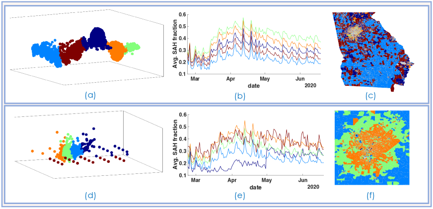
Figure 1: Analysis of adherence to social distancing measures during the COVID-19 pandemic using the dataset (?), which is a collection of geolocation information from mobile devices in the United States, aggregated at the census block group (CBG) level and recorded daily for a period of over a year. As previously studied in Ref. (?), we compute the stay-at-home (SAH) fraction as a simple metric of adherence to social distancing from this data (see SM, LABEL:SM-sec:app for details). To compare with Ref. (?) we consider data for the state of Georgia (GA) and limit it to a 117-day time period, which provides a snapshot of mobility patterns during the first four months of the pandemic. We consider 5509 CBGs within the state, thus our dataset $X_{N}$ has $N=5509$ samples, each of dimension 117. Our workflow on this dataset creates associations between samples based on data-driven geometric optics and produces a sparse graph $\mathcal{X}_{N}$ that is amenable to $3$D embedding (see Figure 4). We do $k$-means clustering on this embedding with $k=5$ set by Ref. (?), for comparison. One application involves using the expected position $\bar{x}_{t}$ to associate a point distance $t$ away from a given sample point $x_{j}\in X_{N}$ and another involves using the maximum position $\hat{x}_{t}$; the details of construction, theory, interpretation and convergence of this framework are discussed below. Top (a,b,c): Embedding of $\mathcal{X}_{N}$ and clustering using $\bar{x}_{t}$. Bottom (d,e,f): Embedding and clustering using $\hat{x}_{t}$. (a) and (d) show $3$D embeddings of $\mathcal{X}_{N}$ and clusters of the resulting points coded by color. (b) and (e) show the average SAH fraction time series for each cluster. In (b) we see a clear separation of clusters by their SAH behavior, and in (e) we have identified an anomalous SAH pattern (in dark blue) in one of the clusters. (c) and (f) color code the CBGs in GA according to the cluster they belong to. (c) shows a clear rural-urban divide in degree of social distancing behavior, and (f) is a magnification of the Atlanta metropolitan region, because many of the outlier CBGs identified are located in this area. See SM, LABEL:SM-sec:app for further details of analysis, including parameter values.

The dataset just considered is an example of the following more general scenario: an experimentalist obtains a sequence of measurements, each consisting of a value for $D$ variables. Each measurement is thus a point in $\mathbb{R}^{D}$. Of course, measurements coming from nature are bound by physical laws, so in fact one must imagine that the true ambient space is some other, nonlinear structure $\mathcal{M}$, residing in $\mathbb{R}^{D}$. Moreover, if the experiment is governed by a number of parameters, then these give $\mathcal{M}$ its local degrees of freedom around any given measurement. This principle is in fact often studied and known as the manifold hypothesis (MH) (?): measurements of arbitrarily high dimensions (residing in $\mathbb{R}^{D}$) arising from natural processes are confined to low-dimensional manifolds (i.e., $\mathcal{M}\subset\mathbb{R}^{D}$ with $\dim\mathcal{M}\ll D$). Due to the MH, the experimentalist’s aim of connecting model parameters to observations through the relationships among measurements is just the analysis of the organizational structure, or geometry of data. In the natural sciences, such analyses are commonly performed through dimensionality reduction, classification, etc. using techniques such as principal component analysis (PCA), t-distributed stochastic neighbor embedding (t-SNE), or variants of Laplacian eigenmaps, that indirectly probe the geometry of data, e.g., (?, ?, ?). In addition, it has recently been appreciated that understanding and exploiting the structure of data, and sometimes reorganizing/reparameterizing it, has advantages in learning frameworks such as convolutional neural networks, e.g., (?, ?). While the state-of-the-art in learning the structure and organization of data is founded on principles of Markovian dynamics (?, ?) – primarily because of their local nature that forms an accessible link between random walks and Markov processes – in practice, these are suitable only for accessing coarse features of the data due to the slowly varying nature of the steady-states that form the basis of these techniques. We have found – as in Figure 1 and the applications in the SM, LABEL:SM-sec:eg – that to perform a fine-scaled data analysis, it is advantageous to shift the paradigm to quantum mechanics, which provides a natural way to formulate dynamics on the data that respects limits to resolution of its geometric structure set by data sampling, through the introduction of a characteristically quantum mechanical uncertainty principle.

1:Inputs: $X_{N}=\{v_{1},...,v_{N}\},v^{*},\epsilon>0,\alpha\geq 1,t>0$ 2:Output: Propagated state $[\psi_{h}^{\zeta}](t)$ 3:procedure Propagate 4:    for $i,j=1:N$ do $\left[T_{\epsilon}\right]_{i,j}\leftarrow k(\nicefrac{{||v_{i}-v_{j}||^{2}}}{{\epsilon}})$ 5:    $D_{\epsilon}\leftarrow\operatorname{diagonal\,matrix}\left(\sum_{j=1}^{N}[T_{\epsilon}]_{i,j}\right)_{1\leq i\leq N}$ 6:    $\Delta_{\epsilon,N}\leftarrow\frac{4(I_{N}-D_{\epsilon}^{-1}T_{\epsilon})}{\epsilon}$ 7:    $U_{\epsilon,N}^{t}\leftarrow\exp(-it\sqrt{\Delta_{\epsilon,N}})$ 8:    $h\leftarrow\epsilon^{\frac{1}{(2+\alpha)}}$ 9:    $p_{0}\leftarrow v_{j}-v^{*}$ for $v_{j}$ closest to point $v^{*}$ 10:    while $1\leq\ell\leq N$ do 11:         $[\psi^{\zeta}_{h}]_{\ell}\leftarrow e^{-\nicefrac{{||v_{\ell}-v^{*}||^{2}}}{{2h}}}e^{\frac{i}{h}(v_{\ell}-v^{*})^{\sf T}\nicefrac{{p_{0}}}{{||p_{0}||}}}$      12:    return $[\psi^{\zeta}_{h}](t)=U^{t}_{\epsilon,N}[\psi^{\zeta}_{h}]$ List of Algorithms 1 Pseudocode for algorithm that performs data-driven propagation of coherent states on a data graph. The inputs are the dataset $X_{N}\subset\mathbb{R}^{D}$, an initial data point to propagate from, $v^{*}$, parameters $\epsilon>0,\alpha\geq 1$, and a time to propagate for, $t>0$. Lines 4-7 construct a data-driven quantum propagator, $U^{t}_{\epsilon,N}$ using a graph Laplacian $\Delta_{\epsilon,N}$ computed from the data. In line 4, $k(\cdot)$ is an exponentially decaying function of the argument and in line 6, $I_{N}$ is the $N\times N$ identify matrix. Lines 10-11 form the $N\times 1$ vector that approximates a coherent state at phase space point $\zeta:=(v^{*},\nicefrac{{p_{0}}}{{||p_{0}||}})$. A more detailed description of this algorithm, and extensions of it, are presented in the SM, LABEL:SM-app:code.

Our implementation is built upon the simulation of quantum dynamics on data as sketched in Algorithm 1. The fundamental relationship connecting this dynamics to the structure of data is given by a discrete quantum-classical correspondence principle (QCC), which is established in Ref. (?) and summarized in the SM, LABEL:SM-sec:method-theory, and applies when the MH holds for the data in $\mathbb{R}^{D}$, confined to $\mathcal{M}$ a smooth, compact, boundaryless submanifold. This relationship is supported by the (traditional) continuum form of the QCC, which physically in our geometric setting connects the propagation of wavefunctions of photons (quantized excitations) on curved space ($\mathcal{M}$) with geodesic propagation of light rays (?). Such a propagation is illustrated in green in Figure 2. More formally, it is a well-known result in microlocal analysis (?, ?) that the trajectory of an impulse $\delta_{x^{*}}$ at $x^{*}\in\mathcal{M}$ with respect to the propagation $U^{t}[\delta_{x^{*}}]:=e^{-it\sqrt{\Delta}}[\delta_{x^{*}}]$, where $\Delta$ is the Laplace-Beltrami operator of $\mathcal{M}$, has singular support along geodesics in all directions at distance $|t|<T$ from $x^{*}$, for a bounded time $T$. This is the continuum QCC in action: it connects the quantum mechanical propagation $U^{t}[\delta_{x^{*}}]$ generated by the quantization $\sqrt{\Delta}$ of the pure kinetic energy classical Hamiltonian, to the geodesic flow, by moving the energy concentration of the singular state $\delta_{x^{*}}$ to time $t$ along the classical flow in directions of the initial state’s asymptotically large momenta (?). The energy concentration propagates to all geodesics at time $t$ emanating from $x^{*}$ because the initial state $\delta_{x^{*}}$ has asymptotically large momenta in all directions.

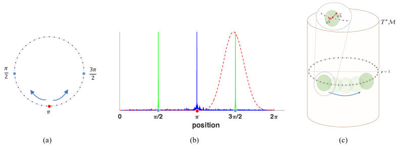
Figure 2: (a) Data is $N=2500$ regularly spaced samples from the unit circle: $x_{j}=(\cos\theta_{j},\sin\theta_{j})$ for $\theta_{j}\in[0,2\pi)$. (b) We observe the squared magnitude of: (green) an undirected optical ray from $x^{*}=\pi$ at time $t=\frac{\pi}{2}$, i.e., $|U^{t}[\delta_{\pi}]|^{2}$, and (blue) the corresponding data-driven quantum propagation, i.e., $|U_{\epsilon,N}^{t}[\delta_{\pi}]|^{2}$. While the former is concentrated at $x_{-}=\pi-t=-\nicefrac{{\pi}}{{2}},x_{+}=\pi+t=\nicefrac{{3\pi}}{{2}}$, which are points that minimize $|d_{g}(x^{*},x)-t|$ ($d_{g}$ is geodesic distance), the latter state bears no resemblance to geodesic propagation, with significant attenuation over the green signal, and an undiminished peak at the source, $x^{*}$. We also show (dashed red) the data-driven propagation of a coherent state centered at $x^{*}$ with uncertainty parameter $h$, i.e., $|U_{\epsilon,N}^{t}[\psi^{\zeta}_{h}]|^{2}$, with $\zeta=(\pi,1)$. This state is approximately centered at the point $x_{+}$, and in fact, its expected position, $\langle x\rangle$, satisfies $|\langle x\rangle-x_{+}|\leq h$. Note that all curves are normalized to have the same maximum value in order to plot them on the same scale. (c) Depiction of coherent state propagation in phase space, $T^{*}\mathcal{M}$. The zoom-in schematically shows $\sqrt{\epsilon}$ and $\sqrt{h}$, the data-determined scale and uncertainty parameters, respectively.

Coming back to quantum dynamics on the data, we couple the above continuum QCC with the now well-known result that, assuming the MH, we can approximate from $N$ measurement samples $X_{N}:=\{v_{1},\ldots,v_{N}\}\subset\mathbb{R}^{D}$ the Laplace-Beltrami operator of their underlying manifold through the graph Laplacian $\Delta_{\epsilon,N}$ of a $\sqrt{\epsilon}$-nearest-neighbour ($\sqrt{\epsilon}$-n.n.) graph on $X_{N}$ with high probability. This is founded on the above-mentioned Markovian methods: in fact, $\Delta_{\epsilon,N}$ is a first-order approximation, in $\epsilon$, to the generator of a Markov process on $X_{N}$, which almost surely limits to a continuum Markov process on $\mathcal{M}$ as $N\to\infty$ (?, ?, ?). Combined with some essential new ingredients, a data-driven approximation to the quantum mechanical propagator $U^{t}$ is given with high probability, in Ref. (?), by the $N\times N$ matrix $U_{\epsilon,N}^{t}:=e^{-it\sqrt{\Delta_{\epsilon,N}}}$, see line 7 of Algorithm 1.

Given this construction, it is tempting to reproduce the geodesic propagation of light rays given through $U^{t}[\delta_{x^{*}}]$ with $U_{\epsilon,N}^{t}[\delta_{x^{*}}]$ . However, as shown in the blue curve in Figure 2(b), this data-driven propagation bears no resemblance to the continuum signal $U^{t}[\delta_{x^{*}}]$ (green curve). To see why this is, we go back to the Markov process roots of $U^{t}_{\epsilon,N}$: namely, the Markov process defining $\Delta_{\epsilon,N}$ is discretized to $\sqrt{\epsilon}$-balls on the manifold. Then, based on the uncertainty principle, the analysis in (?) shows that this Markov process acts like a low-pass filter by attenuating spatial frequencies with magnitude $\gtrsim 1/\sqrt{\epsilon}$. Therefore, $\Delta_{\epsilon,N}$ approximates a scalar operator at bandwidth $\gtrsim 1/\sqrt{\epsilon}$ and by virtue of being its spectral function, so does $U_{\epsilon,N}^{t}$. This explains the concentration of the blue curve in Figure 2(b) about $x^{*}$ and predicts that this behaviour will persist even in the limit $N\to\infty$ while $\epsilon>0$ remains bounded away from zero.

Understanding this issue is the fulcrum of our discrete QCC, which recovers light rays from data-driven simulation of quantum dynamics. As we have seen, the primary obstruction to approximating the continuum QCC with $U_{\epsilon,N}^{t}[\delta_{x^{*}}]$ is the over-concentration of the initial state $\delta_{x^{*}}$, which gives frequency content above the data-determined threshold $\sim 1/\sqrt{\epsilon}$. To control this, we introduce a state $\psi_{h}\in C^{\infty}(\mathcal{M}\times(0,1]_{h})$ surrogate to $\delta_{x^{*}}$, whose bandwidth we can control to scale as $\sim 1/h$ and whose continuum propagation $U^{t}[\psi_{h}]$ follows the light ray emanating from $x^{*}$ until time $t$, to within a $\sqrt{h}$-ball throughout the propagation. This is satisfied by coherent states, which in the continuum have position-space representation: $\psi_{h}^{\zeta}(v):=e^{-\frac{1}{2h}||v-x^{*}||^{2}}e^{\frac{i}{h}\langle v-x^{*},p\rangle}$ with position $x^{*}\in\mathcal{M}$ and momentum $p\in T^{*}_{x^{*}}\mathcal{M}$. In particular, $\psi_{h}^{\zeta}$ (time $t=0$) is localized in phase space in a $\sim\sqrt{h}$-ball about the point $\zeta:=(x^{*},p/h)\in T^{*}\mathcal{M}$. The wave-particle duality is apparent in this state: its spatial oscillation frequency is set by $p/h$, where $p$ is the classical momentum vector which sets the direction of maximum variation. Thus, the uncertainty parameter $0<h\leq 1$ governing the quantum mechanical properties of coherent states gives us the desired control to establish our discrete QCC.

The finite discretization of $\psi_{h}^{\zeta}$ can be defined on the sampled dataset $X_{N}$ as a vector $[\psi_{h}^{\zeta}]$ of dimension $N\times 1$ as per line 10 of Algorithm 1, and its extensions in SM, LABEL:SM-app:code. We approximate the momentum $p$ from the data $X_{N}$ using various techniques that approximate the tangent space at a given $x^{*}\in X_{N}$, and show in SM, LABEL:SM-sec:geodesic-measurements. In order for the data-driven propagation $U_{\epsilon,N}^{t}[\psi_{h}^{\zeta}]$ to approximate $U^{t}[\psi_{h}^{\zeta}]$ and therefore, to follow the light rays on data, the bandwidth $1/h$ must be kept $\ll 1/\sqrt{\epsilon}$. Hence, crucially we scale $h\gg\sqrt{\epsilon}$. The convergence rates in [(?) and SM, LABEL:SM-sec:data_dyn] that take into account the finite size $N$ of the dataset, establish that the parameter $h(N)$ dictates how the uncertainty in the fine-scaled resolution of the geometry of the dataset scales with $N$.

In Figure 2(b) the dashed red line shows the result of propagating a coherent state using a data-driven propagator for the circle example. By incorporating the intrinsic uncertainty induced by finite sampling into the formulation of quantum dynamics, we recover accurate propagation. In Figure 2(c) we also depict coherent state propagation in phase space for this example, and graphically show the relationship between $\epsilon$ and $h$. We stress that this uncertainty relation crucially depends on the quantum formulation that realizes the graph Laplacian at length scale $\epsilon$ as a quantization of the geodesic Hamiltonian up to wavelength $h$ (this is further explained with detail in (?)).

The coherent states just considered are meaningful for the data: their localization and momentum properties jointly encode the local density and variation of the data samples. The MH can be interpreted as a combined, local and global hypothesis on these properties of the dataset: it dictates that as more data samples are acquired from measurements of a physical system, their variation and concentration in ambient space are subject to geometric constraints, which are fixed by the natural process and thus independent of the number of measurements. The discrete QCC realized by $U_{\epsilon,N}^{t}[\psi_{h}^{\zeta}]$ extends the local information encoded in $\psi_{h}^{\zeta}$ non-locally to find optimal paths and lengths between data points at a sufficiently large $N$, with respect to the constraints governed by the system being measured. It is remarkable that this simulated quantum dynamics on the data, with finite samples, traverses the optimal path by forecasting new measurements that are feasible for the underlying physical system.

In the SM we derive the convergence results to establish the following: given $N$ data samples, $X_{N}$, from a smooth density on $\mathcal{M}$, the data-driven finite-dimensional matrix propagation $[\psi_{h}^{\zeta}](t):=U_{\epsilon,N}^{t}[\psi_{h}^{\zeta}]$ returned by Algorithm 1, with $h\propto\epsilon^{\frac{1}{2+\alpha}}$ for $\alpha\geq 1$ agrees with $U^{t}[\psi_{h}^{\zeta}]$ up to uniform error $O(h)$ w.h.p., provided $h\gtrsim N^{-\frac{1}{\gamma}}$ for $\gamma>0$ a constant depending only on $\alpha$ and $\dim\mathcal{M}$. Thus, $[\psi_{h}^{\zeta}](t)$ traverses within an $O(\sqrt{h})$ radius of the geodesic beam emanating from $v^{*}$ in the direction $p$ to time $t$. Moreover, the point $\bar{x}_{t}:=||\psi_{h}^{\zeta}(t)||^{-2}\sum_{j=1}^{N}\begin{pmatrix}v_{j,1}&\cdots&v_{j,D}\end{pmatrix}|[\psi_{h}^{\zeta}](t)|^{2}$, which is the expected position of the propagated state, is w.h.p. within geodesic distance $O(h)$ to the point $x^{*}_{t}$, that is geodesic distance $t$ from the initial position $v^{*}$ in the direction $p$. While this expected value of the position coordinate, $\bar{x}_{t}$, is the best estimate of position along the geodesic path, due to the localization of the propagated state the maximum of the wavepacket distribution, $\hat{x}_{t}:=\arg\max|[\psi_{h}^{\zeta}](t)|^{2}$ is also w.h.p. within geodesic distance $O(h)$ from $x^{*}_{t}$ (?).

The fine-scaled resolution properties of quantum dynamics on data are now apparent: geodesics are inherently high-frequency features of the data (?). While Markovian methods have introduced a crucial $\epsilon$ dependence in data analysis, which signifies that the quality of approximation of $\Delta_{\epsilon,N}$ is tied to a random walker’s traversibility of the underlying $\sqrt{\epsilon}$-n.n. graph (?), we have switched the perspective to a quantum mechanical wavelength $h$ at which the dataset’s fine-scaled geometry can be resolved.

The uncertainty principles utilized above to study the geometry of data through the crucial $h(\epsilon)$ relationship, can also be viewed from a signal processing perspective. In fact, quantum mechanics in the continuum and time-frequency analysis are two sides of the same coin, and share common notions of uncertainty principles (?). Particularly relevant to this work is the short-time Fourier transform (STFT) and its relation to localized wavepackets.

To bring our results firmly into the signals processing setting, we begin by noting that our initial coherent states $\psi_{h}^{\zeta}$ are actually Gabor wavelets (?). These wavelets define a form of the STFT, namely $T_{h}:\mathcal{D}(\mathcal{M})\to C^{\infty}(T^{*}\mathcal{M})$ that maps a distribution $f\in\mathcal{D}$ to its time-frequency (or phase space) representation by integrating against $\overline{\psi^{\zeta}_{h}}$. Since this STFT’s window function saturates the time-frequency uncertainty, this is just the Gabor transform adapted to a manifold and frequency scaled by a factor of $1/h$. The Gabor spectrogram $|T_{h}[f](\zeta)|^{2}$ is an essential tool for signal analysis and especially detection, since it gives a picture of the frequency content of $f$ occurring across spatial windows with equal order of resolution in space (position) and frequency, which in our case is a $\sqrt{h}$-ball in phase space. In practice, we realize this spectrogram from just the measurement samples $X_{N}=\{v_{1},\ldots,v_{N}\}\subset\mathbb{R}^{D}$ by taking directions $p$ from an approximate tangent space at each $v_{j}$ and computing $\zeta:=(x_{j},p)\mapsto T_{h,N}[f](\zeta):=[\psi_{h}^{\zeta}]^{\dagger}[f]$. We show in the SM, LABEL:SM-sec:dual that with $\zeta$ taken in this way, $\mathscr{T}_{h}^{t}:\zeta\mapsto|T_{h,N}[U_{\epsilon,N}^{-t}[\delta_{x^{*}}]](\zeta)|^{2}$ approximates w.h.p., to within $O(h)$ error, the spectrogram of $U^{-t}[\delta_{x^{*}}]$ uniformly over any bounded region $\mathcal{B}$ of phase space at bandwidths $O(1/h)$, provided that $h\gg\sqrt{\epsilon}$. Since as discussed above, $U^{-t}[\delta_{x^{*}}]$ has light rays emanating from $x^{*}$ in all possible directions on $\mathcal{M}$, these can be computationally recovered from $\mathscr{T}_{h}^{t}$ evaluated on a region $\mathcal{B}$ containing all unit speed phase space points. More specifically, our use of the Gabor transform and the relationship between uncertainty and sampling density given by $h(\epsilon)$ show that the high-frequency content of $U^{-t}[\delta_{x^{*}}]$ is attenuated to within frequency band $1/h\ll 1/\sqrt{\epsilon}$ and spread across phase space windows with radius of order $\sqrt{h}\gg\epsilon^{\frac{1}{4}}$. For this reason, we view $U^{-t}[\delta_{x^{*}}]$ as a signal with arbitrarily high-frequency content that is attenuated to $U_{\epsilon,N}^{-t}[\delta_{x^{*}}]$ by the finite sampling that gives the dataset $X_{N}$.

To illustrate this dual picture, we present spectrograms for the circle example from Figure 2 at a fixed propagation time and various resolutions, $h$, in Figure 3. When $h\lesssim\sqrt{\epsilon}$ the inaccuracy of the propagation is evident. This is another perspective on the observation from Figure 2, where the direct application $U_{\epsilon,N}^{t}[\delta_{x^{*}}]$ is unable to recover the propagated state due to the attenuation of high-frequency content in the signal discussed above in terms of quantum dynamics. Whereas, when the resolution of the spectrogram is at $h\gg\sqrt{\epsilon}$ the signal $U^{t}[\delta_{x^{*}}]$ is recovered.

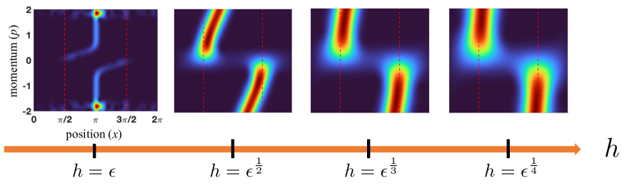
Figure 3: Illustrating the dual picture of resolving time evolved states at scales set by $h$. We propagate an initial impulse $\delta_{\pi}$ on sampled circle (as in Figure 2, with $N=2500$) with the data-driven propagator $U_{\epsilon,N}^{t}$ for $t=\nicefrac{{\pi}}{{2}}$. Each plot shows the discrete approximation $\mathscr{T}_{h}^{t}(x,p)$ to the spectrogram of this state at varying resolution $h$ as a function of $\epsilon$, the scale parameter set by the data sampling. At resolutions $h\lesssim\sqrt{\epsilon}$ the spectrogram’s localization is inaccurate in terms of the high-frequency content $U^{t}[\delta_{\pi}]$ (red, dashed lines), while at appropriate resolutions, $h=\epsilon^{\nicefrac{{1}}{{(2+\alpha)}}}$, for $\alpha>1$, we see a state localized at $x^{*}\pm t=\pi\pm\nicefrac{{\pi}}{{2}}$ and delocalized in momentum, as we would expect from a propagating a state perfectly localized in position space. This illustrates (1) the interpretation of $h$ as setting the scale at which data-driven dynamics can be accurately resolved, and (2) that the spectrogram reveals at once, the position at time $t$ of light-rays emanating from $x^{*}$ in all possible directions.

The data-driven quantum dynamics formulated above enables estimation of intrinsic distances between points in a dataset: if $\bar{x}_{t}(j;p_{j})\in X_{N}$ denotes the data point closest to $\bar{x}_{t}$ (or $\hat{x}_{t}$) computed as above with respect to an initial state $\psi_{h}^{\zeta}$ localized at $\zeta:=(v_{j},p_{j})$, then $t$ gives the propagation time of a coherent state following approximately a ray emanating in direction $p_{j}$ from $v_{j}$. When the data is sampled from a smooth density on a smooth, compact, boundaryless manifold, we have established that $t$ is w.h.p., within $O(h)$ of the geodesic distance . In fact, by using local PCA to define $\psi^{\zeta}_{h}$ and hence, $p_{j}$, we can chart the dataset $X_{N}$ with geodesic polar coordinates (GPC), or equivalently, normal coordinates (SM LABEL:SM-sec:state-prep). We pause to emphasize that the procedure we have described gives access to geodesics and GPC on a manifold, which are inherently described by non-linear dynamical equations, through linear, matrix computations. Computing such quantities, even when much more is known about the manifold, is generally computationally difficult since typical approximation methods are insufficient: polyhedral approximations are not a faithful model of manifolds with curvature restrictions (?) and even forward marching type approximations are known to be prone to failures (?). Furthermore, our result establishes the first general convergence result for geodesics and GPC from data.

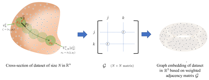
Figure 4: Illustration of how data-driven extraction of geodesic distances between data points establishes a similarity metric on the dataset that can be used to perform low-dimensional embedding of the data. By propagating a coherent state centered on $x_{j}$, with initial momentum $p_{j}$ ($|p_{j}|=1$), with $U_{\epsilon,N}^{t}$, and extracting the point closest to the expected position of the resulting state, $x_{k}\equiv\bar{x}_{t}(j,p_{j})$, we establish a distance $t$ between these points (left). Repeating this process for a set of initial point and times allows construction of a matrix $\mathcal{G}$, that approximates geodesic distances between data points (middle). This matrix can be utilized as a weighted adjacency matrix for a (low-dimensional) graph embedding of the dataset (right).

More broadly, the assignment of a data point $\bar{x}_{t}(j,p_{j})=v_{k}$ to a given data point $v_{j}$ is, in itself, independent of further structural assumptions on the dataset. Even when the data $X_{N}$ is not guaranteed to be sampled from a manifold, this defines a distance relationship between two points based on the quantum walk $U_{\epsilon,N}^{t}[\psi_{h}^{\zeta}]$. Based on this distance relationship we can build an $N\times N$ adjacency matrix, $\mathcal{G}$, for a graph $\mathcal{X}_{N}$ on $X_{N}$, with elements $\mathcal{G}_{j,k}=\mathcal{G}_{k,j}=t$; see Figure 4. Repeating this process for a collection of initial points $v_{j}$ and time-steps, $t_{1},\ldots,t_{m}$ populates this adjacency matrix, which captures a notion of distance between the data points in $X_{N}$ given by the quantum propagation times of coherent states. We can perform emebeddings of $\mathcal{X}_{N}$ to achieve tasks such as recovering reduced-dimensional coordinates, clustering, classification, etc. We find that even the most classical embedding of $\mathcal{X}_{N}$ in few dimensions, such as the Fruchterman-Reingold (FR) method of springs and electrostatic forces (?), recovers salient features of complex datasets. For example, Figure 1 shows examples of FR embedding into 3 dimensions followed by $k$-means clustering of the COVID-19 mobility information dataset.

We have argued that, similar to the Fourier transform being fundamental for signal analysis, quantum propagation and sensing are fundamental for structure analysis in sampled data. Figure 1 exhibits the ability of this approach to organize and discover previously unseen anomalous behavior in social distancing data collected during the COVID-19 crisis, affected by irregularity and noise and generated by complex, intractable mobility dynamics. As seen from Algorithm 1 the basic transformation of data realizing this approach is algorithmically quite simple, involving only linear operations, and moreover, we have rigorous justification with rates of convergence and mild assumptions that are supported from our novel inclusion of graph Laplacians in the framework of semiclassical analysis and probabilistic reasoning. Furthermore, we have shown both sides of a dual picture, providing interpretations through the QCC on the one hand and signals processing on the other, as exhibited in Figures 2 and 3, respectively, which are again firmly grounded mathematically through probabilistic convergence rates. In the SM we present several additional applications – combined with the graph embedding method depicted in Figure 4 – even for meaningful organization of very small datasets, and a statistical analysis of the quality of geodesic extraction on model manifolds, with the corresponding algorithms. Our approach to data analysis combines methods from a wide array of fields, including dynamics, geometric inverse problems, statistics and physics, and has relationships to yet more disciplines, which we discuss in some detail in the SM, LABEL:SM-sec:disc.

See pages - of SM.pdf

References

- 1. S. B. Damelin, W. Miller, Jr., The mathematics of signal processing, Cambridge Texts in Applied Mathematics (Cambridge University Press, Cambridge, 2012).
- 2. J. Wright, Y. Ma, High-Dimensional Data Analysis with Low-Dimensional Models: Principles, Computation, and Applications (Cambridge University Press, 2022).
- 3. C. M. Bishop, Pattern recognition and machine learning, Information Science and Statistics (Springer, New York, 2006).
- 4. E. Candes, R. R. Coifman, A. Singer, T. Strohmer, Applied Harmonic Analysis, Massive Data Sets, Machine Learning, and Signal Processing (2019). Workshop Report from ”Computational Harmonic Analysis and Data Science”. Banff International Research Station.
- 5. A. Glielmo, et al., Chemical Reviews 121, 9722 (2021).
- 6. Safegraph Inc. Social Distancing Metrics, https://docs.safegraph.com/docs/social-distancing-metrics (2021).
- 7. R. Levin, D. L. Chao, E. A. Wenger, J. L. Proctor, Nature Computational Science 1, 588 (2021).
- 8. C. Fefferman, S. Mitter, H. Narayanan, J. Amer. Math. Soc. 29, 983 (2016).
- 9. R. R. Coifman, et al., Proceedings of the National Academy of Sciences 102, 7426 (2005).
- 10. M. Maggioni, Notices Amer. Math. Soc. 62, 1185 (2015).
- 11. D. Kobak, P. Berens, Nature Communications 10, 5416 (2019).
- 12. W. Zhu, et al., arXiv:1711.06246 [cs] (2017).
- 13. M. M. Bronstein, J. Bruna, T. Cohen, P. Veličković, arXiv:2104.13478 [cs, stat] (2021).
- 14. M. Belkin, P. Niyogi, Neural Computation 15, 1373 (2003).
- 15. R. R. Coifman, S. Lafon, Appl. Comput. Harmon. Anal. 21, 5 (2006).
- 16. A. Kumar, On a quantum-classical correspondence: from graphs to manifolds (2021). ArXiv:2112.10748.
- 17. D. Gloge, D. Marcuse, JOSA 59, 1629 (1969).
- 18. S. Zelditch, Eigenfunctions of the Laplacian of Riemannian manifolds (Am. Math. Soc., 2017).
- 19. M. Zworski, Semiclassical analysis, vol. 138 of Graduate Studies in Mathematics (American Mathematical Society, Providence, RI, 2012).
- 20. M. Hein, J.-Y. Audibert, U. von Luxburg, Learning theory (Springer, Berlin, 2005), vol. 3559 of Lecture Notes in Comput. Sci., pp. 470–485.
- 21. K. Gröchenig, Foundations of time-frequency analysis, Applied and Numerical Harmonic Analysis (Birkhäuser Boston, Inc., Boston, MA, 2001).
- 22. J.-P. Antoine, Operator algebras and mathematical physics, T. Bhattacharyya, M. A. Dritschel, eds. (Springer International Publishing, 2015), pp. 123–156.
- 23. A. Petrunin, Turkish Journal of Mathematics 27, 173 (2003).
- 24. G. Peyré, M. Péchaud, R. Keriven, L. D. Cohen, Foundations and Trends in Computer Graphics and Vision 5, 197 (2010).
- 25. T. M. J. Fruchterman, E. M. Reingold, Software: Practice and Experience 21, 1129 (1991).