Probably Approximate Shapley Fairness with Applications in Machine Learning

Abstract

The Shapley value (SV) is adopted in various scenarios in machine learning (ML), including data valuation, agent valuation, and feature attribution, as it satisfies their fairness requirements. However, as exact SVs are infeasible to compute in practice, SV estimates are approximated instead. This approximation step raises an important question: do the SV estimates preserve the fairness guarantees of exact SVs? We observe that the fairness guarantees of exact SVs are too restrictive for SV estimates. Thus, we generalise Shapley fairness to probably approximate Shapley fairness and propose fidelity score, a metric to measure the variation of SV estimates, that determines how probable the fairness guarantees hold. Our last theoretical contribution is a novel greedy active estimation (GAE) algorithm that will maximise the lowest fidelity score and achieve a better fairness guarantee than the de facto Monte-Carlo estimation. We empirically verify GAE outperforms several existing methods in guaranteeing fairness while remaining competitive in estimation accuracy in various ML scenarios using real-world datasets.

1 Introduction

The Shapley value (SV) is widely used in machine learning (ML), to value and price data (Agarwal, Dahleh, and Sarkar 2019; Ohrimenko, Tople, and Tschiatschek 2019; Ghorbani and Zou 2019; Ghorbani, Kim, and Zou 2020; Xu et al. 2021b; Kwon and Zou 2022; Sim, Xu, and Low 2022; Wu, Shu, and Low 2022), value data contributors in collaborative machine learning (CML) (Sim et al. 2020; Tay et al. 2022; Agussurja, Xu, and Low 2022; Nguyen, Low, and Jaillet 2022) and federated learning (FL) (Song, Tong, and Wei 2019; Wang et al. 2020; Xu et al. 2021a) to decide fair rewards, and value features’ effects on model predictions for interpretability (Covert and Lee 2021; Lundberg and Lee 2017). We consider data valuation as our main example. Given a set $N$ of $n$ training examples and a utility function $v$ that maps a set $P$ of training examples to a real-valued utility (e.g., test accuracy of an ML model trained on $P$), the SV $\phi_{i}$ of the $i$-th example is

$$\phi_{i}=\phi_{i}(N,v) \coloneqq 1/(n!)\textstyle\sum_{\pi\in\Pi}\sigma_{i}(\pi)$$ (1)

$$\sigma_{i}(\pi) \coloneqq v(P_{i}^{\pi}\cup\{i\})-v(P_{i}^{\pi})$$

where $\pi$ is a permutation of the $N$ training examples and $\Pi$ denotes the set of all possible permutations. The SV for the $i$-th example is its average marginal contribution, $\sigma_{i}(\pi)$, across all permutations. The marginal contribution $\sigma_{i}(\pi)$ measures the improvement in utility (e.g., test accuracy) when the $i$-th example is added to the predecessor set $P_{i}^{\pi}$ containing all training examples $j$ preceding $i$ in $\pi$.

The wide adoption of SV is often justified through its fairness axiomatic properties (recalled in Sec. 2). In data valuation, SV is desirable as it ensures that any two training example that improves the ML model performance equally when added to any data subset (i.e., all marginal contributions are equal) are assigned the same value (known as symmetry). However, a key downside of SV is that the exact calculation of $\phi_{i}$ in Equ. (1) has exponential time complexity and is intractable when valuing more than hundreds of training examples (Ghorbani and Zou 2019; Jia et al. 2019). Existing works address this downside by viewing the SV definition in Equ. (1) as an expectation over the uniform distribution $U$ over $\Pi$, $\phi_{i}=\mathbb{E}_{\pi\sim U}[\sigma_{i}(\pi)]$, and applying Monte Carlo (MC) approximation (Castro, Gómez, and Tejada 2009) with $m_{i}$ randomly sampled permutations, thus $\phi_{i}\approx\varphi_{i}\coloneqq 1/m_{i}\sum_{t=1}^{m_{i}}\sigma_{i}(\pi^{t}),\pi^{t}\sim U$ (Ghorbani and Zou 2019; Jia et al. 2019; Song, Tong, and Wei 2019).

However, this approximation creates an important issue — (i) do the fairness axioms that justify the use of Shaplay value still hold after approximation (Sundararajan and Najmi 2020; Rozemberczki et al. 2022)? The answer is unfortunately no as we empirically demonstrate that the symmetry axiom does not hold after approximations in Fig. 2. For two identical training examples, their (approximated) SVs used in data pricing are not guaranteed to be equal. We address this unresolved important issue by proposing the notion of probably approximate Shapley fairness for SV estimates $\varphi_{i}$, for every $i\in N$. As the original fairness axioms are too restrictive, in Sec. 3, we relax the fairness axioms to approximate fairness and consider how they can be satisfied with high probability. We introduce a fidelity score (FS) to measure the approximation quality of $\varphi_{i}$ w.r.t. $\phi_{i}$ for each example $i$ and provide a fairness guarantee dependent on the worst/lowest fidelity score across all training examples.

In data valuation, computing the marginal contribution of an $i\in N$ in any sampled permutation is expensive as it involves training model(s). (ii) How do we achieve probably approximate Shapley fairness with the lowest budget (number of samples) of marginal contribution evaluations? While it is difficult to achieve the highest approximate fairness possible, we show that we can instead achieve a high fairness guarantee (i.e., a lower bound to probably approximate Shapley fairness) via the insight that the budget need not be equally spent on all training examples. For example, if the marginal contribution of example $i$, $\sigma_{i}(\pi^{t})$ in many sampled permutations are constant, we should instead evaluate that of example $j$ with widely varying $\sigma_{j}(\pi^{t})$ sampled so far. Our method may use a different number of marginal contribution samples, $m_{i}$, for each example $i$ and greedily improve the current worst fidelity score across all training examples.

Lastly, to improve the fidelity score, we novelly use previous samples, i.e., evaluated marginal contribution results, to influence and guide the current sampling of permutations. In existing MC methods (Owen 1972; Okhrati and Lipani 2020; Mitchell et al. 2022) the sampling distribution that generates $\pi$ is pre-determined and fixed across iterations. In our work, we use importance sampling to generate $\pi$ for $\varphi_{i}$ as it supports using an alternative proposal sampling distribution, $q_{i}(\pi)$. For any example $i$, we constrain permutations $\pi$ with predecessor set of equal size to have the same probability $q_{i}(\pi)$. The parameters of the sampling distribution $q_{i}$ are actively updated across iterations and learnt from past results (i.e., tuples of predecessor set size and marginal contribution) via maximum likelihood estimation or a Bayesian approach. By doing so, we reduce the variance of the estimator $\varphi_{i}$ as compared to standard MC sampling, thus improving the fidelity scores efficiently and the overall fairness (guarantee).

Our specific contributions are summarized as follows:

• We propose a probably approximate Shapley fairness for SV estimates and exploit an error-aware fidelity score to provide a fairness guarantee via a polynomial budget complexity.

• We design greedy selection, which by iteratively prioritising $\varphi_{i}$ with lowest FS, can obtain the optimal minimum FS given a fixed total budget $m$ and improve the fairness guarantee (Proposition 1).

• We derive the optimal categorical distribution (intractable) for selecting permutations, and obtain an approximation for active permutation selection. We integrate both greedy and active selection into a novel greedy active estimation (GAE) with provably better fairness than MC.

• We empirically verify that GAE outperforms existing methods in guaranteeing fairness while remaining competitive in estimation accuracy in training example and dataset valuations, agent valuation (in CML/FL) and feature attribution with real-world datasets.

2 Preliminaries

Fairness of SV.

SV (Equ. (1)) is often adopted (Agarwal, Dahleh, and Sarkar 2019; Sim et al. 2020; Song, Tong, and Wei 2019; Xu et al. 2021a; Sim, Xu, and Low 2022) for guaranteeing fairness by satisfying several axioms (Chalkiadakis, Elkind, and Wooldridge 2011):

1. Nullity: $(\forall\pi\in\Pi,\sigma_{i}(\pi)=0)\implies\phi_{i}=0$.

2. Symmetry: $(\forall C\subseteq N\setminus\{i,j\},v(C\cup\{i\})=v(C\cup\{j\}))\implies\phi_{i}=\phi_{j}$.

3. Strict desirability (Bahir et al. 1966): $\forall i\neq j\in N,(\exists B\subseteq N\setminus\{i,j\},v(B\cup\{i\})>v(B\cup\{j\}))\wedge(\forall C\subseteq N\setminus\{i,j\},v(C\cup\{i\})\geq v(C\cup\{j\}))\implies\phi_{i}>\phi_{j}$.

Nullity means if a training example does not result in any performance improvement (marginal contribution is $0$ to any permutation), then its value is $0$. It ensures offering useless data does not give any reward (Sim et al. 2020)). Symmetry ensures identical values for identical training examples. Strict desirability implies if $i$ gives a larger performance improvement than $j$ in all possible permutations, then $i$ is strictly more valuable than $j$. We exclude the efficiency axiom as it does not suit ML use-cases (Ghorbani and Zou 2019; Bian et al. 2022; Kwon and Zou 2022), and exclude the linearity (Jia et al. 2019) and monotonicity (Sim et al. 2020) axioms for fairness analysis as we restrict our consideration to one utility function $v$ (Bian et al. 2022). Note that the fairness of exact SV is binary: either satisfying all these axioms or not.

Sampling-based estimations.

These methods typically extend the MC formulation of $\phi_{i}\approx\varphi_{i}\coloneqq\mathbb{E}_{\pi_{t}\sim U}\left[\sigma_{i}(\pi_{t})\right]$ by changing the sampling distribution of $\pi_{t}$. Importantly, in all these methods, for each sampled permutation $\pi_{t}$, a single marginal contribution $\sigma_{i}(\pi_{t})$ is evaluated and used in $\varphi_{i}$. Thereafter, we consistently refer to this single evaluation as expending one budget (i.e., one permutation) and the corresponding marginal contribution $\sigma_{i}(\pi_{t})$ as one sample.

Formally, a sampling-based estimation method estimates $\phi_{i}$ via the expectation of the random variable $\sigma_{i}(\pi)$ (which depends on the permutations randomly sampled according to some distribution $q$): $\phi_{i}\approx\mathbb{E}_{q}[\sigma_{i}(\pi)]$. Hence, such methods differ from each other in the distribution $q$ as well as the selection of entry $i\in N$ to evaluate in each iteration. The estimates $\varphi_{i}$’s can be independent of each other such as MC (Castro, Gómez, and Tejada 2009), and stratified sampling (Maleki et al. 2013; Castro et al. 2017), or dependent such as antithetic Owen method (Owen 1972; Okhrati and Lipani 2020) and Sobol method (Mitchell et al. 2022). We provide theoretical results for both scenarios when the estimates $\varphi_{i}$’s are independent and dependent.

3 Generalised Fairness for Shapley Value Estimates

3.1 Fairness Axioms for Shapley Value Estimates

We propose the following re-axiomatisation of fairness for SV estimates (based on axioms F1-F3) using conditional events, by analysing multiplicative and absolute errors.

1. Nullity: let $E_{A_{1}}$ be the (conditional) event that for any $i\in N$, conditioned on $\phi_{i}=0$, $|\varphi_{i}|\leq\epsilon_{2}$.

2. Symmetry: let $E_{A_{2}}$ be the (conditional) event that for all $i\neq j\in N$, conditioned on $\phi_{i}=\phi_{j}$, then $|\varphi_{i}-\varphi_{j}|\leq(\epsilon_{1}|\phi_{i}|+\epsilon_{2})+(\epsilon_{1}|\phi_{j}|+\epsilon_{2})$.

3. Approximate desirability: let $E_{A_{3}}$ be the (conditional) event that for all $i\neq j\in N$, conditioned on $(\exists B\subseteq N\setminus\{i,j\},v(B\cup\{i\})>v(B\cup\{j\}))\wedge(\forall C\subseteq N\setminus\{i,j\},v(C\cup\{i\})>v(C\cup\{j\}))$, then $\varphi_{i}-\varphi_{j}>-(\epsilon_{1}|\phi_{i}|+\epsilon_{2})-(\epsilon_{1}|\phi_{j}|+\epsilon_{2})$.

Thereafter, satisfying A1-A3 refers to the events $E_{A_{1}}$-$E_{A_{3}}$ occurring, respectively. To see A1-A3 generalise the original axioms F1-F3: A1 requires the SV estimate to be small for a true SV with value $0$ (as in F1); A2 requires the SV estimates for equal SVs be close (generalised from being equal in F2); A3 requires the ordering of $\varphi_{i},\varphi_{i}$ for some $i,j$ from F3 to be preserved up to some error, specifically a multiplicative error $\epsilon_{1}$ (to account for different $|\phi_{i}|$) and an absolute error $\epsilon_{2}$ (to avoid degeneracy from extremely small $|\phi_{i}|$) where F3 has no such error term. Intuitively, smaller errors $\epsilon_{1},\epsilon_{2}$ mean $\bm{\varphi}$ are “closer” (in fairness) to $\bm{\phi}$. In addition, the ratio $\xi\equiv\epsilon_{2}/\epsilon_{1}$ denotes the tolerance (to be set by user) of relative (multiplicative) vs. absolute errors where a larger $\xi$ implies a higher tolerance for absolute error (i.e., favours A1 over A2 & A3) and vice versa. In contrast to existing works that only consider the concentration results of $\varphi_{i}$ w.r.t. $\phi_{i}$ for each $i$ (Castro, Gómez, and Tejada 2009; Castro et al. 2017; Maleki et al. 2013), we additionally consider the interaction between $i,j$ to define the following:

Definition 1 (Probably Approximate Shapley Fairness).

For fixed $\epsilon_{1},\epsilon_{2}$, and some $\delta\in(0,1)$ s.t. $\bm{\varphi}$ satisfy A1-A3 jointly w.p. $\geq 1-\delta$, then we call $\bm{\varphi}$ satisfy $(\epsilon_{1},\epsilon_{2},\delta)$-Shapley fairness.

In Definition 1, $\bm{\varphi}$ are probably (w.p. $\geq 1-\delta$) approximately (w.r.t. errors $\epsilon_{1},\epsilon_{2}$) Shapley fair. Hence, given the error requirements $\epsilon_{1},\epsilon_{2}$, a smaller $\delta$ means a better fairness guarantee. In particular, $\bm{\phi}$ satisfy the optimal $(0,0,0)$-Shapley fairness. Despite the appeal, analysing existing estimators w.r.t. Definition 1 is difficult because most do not come with a direct variance result (elaborated in Appendix B). The only expect is the MC method (Castro, Gómez, and Tejada 2009; Maleki et al. 2013) which we analyse in Sec. 4.

3.2 Fairness Guarantee via the Fidelity Score of Shapley Value Estimates

Inspired by the concept of signal-to-noise ratio (SNR) widely adopted in optics (de Boer et al. 2003) and imaging (Rose 2012), we design a metric for the variation of $\varphi_{i}$, named fidelity score, expressed in Footnote 3.

Definition 2 (Fidelity Score).

The fidelity score (FS) of an (unbiased) SV estimate $\varphi_{i}$ for $\phi_{i}$ is defined as $f_{i}\equiv\text{FS}(\varphi_{i},\epsilon_{1},\epsilon_{2})\coloneqq(|\phi_{i}|+\epsilon_{2}/\epsilon_{1})^{2}/\mathbb{V}[\varphi_{i}]$ where $\mathbb{V}[\varphi_{i}]$ is the variance of $\varphi_{i}$.

The FS exactly matches the SNR in $\varphi_{i}$ when $\epsilon_{2}=0$. A higher $f_{i}$ implies a more accurate $\varphi_{i}$. $f_{i}$ is higher when the variance $\mathbb{V}[\varphi_{i}]$ is small. This occurs when the marginal contributions, $\sigma_{i}(\pi)$, are close for all permutations $\pi\in\Pi$ or when the number of samples $m_{i}$ used to compute $\varphi_{i}$ is large. As $m_{i}\to\infty$, $\mathbb{V}[\varphi_{i}]\to 0$ and $f_{i}\to\infty$. Additionally, we introduce an error-aware term $\xi\coloneqq\epsilon_{2}/\epsilon_{1}$ in the FS numerator to better capture estimation errors and allow examples with SV of $0$ to have different FSs.

Moreover, we empirically verify that $f_{i}$ is a good reflection of the approximation quality and analyze the impact of $\xi$. For the former, we compared $f_{i}$ vs. absolute percentage error (APE) of $\varphi_{i}\coloneqq|(\varphi_{i}-\phi_{i})/\phi_{i}|$. Fig. 1 shows the negative correlation between FS ($f_{i}$) and estimation error (APE) (note that we plot $\text{APE}^{-0.5}$). This will justify our proposal to prioritize improving the estimate $\varphi_{i}$ with the lowest $f_{i}$ in Sec 4.1. For the latter, we compare the correlation between FS, $f_{i}$ and the inverse estimation error, $\text{APE}^{-0.5}$, for different values of $\xi$ in Tab. 1 and find that $\xi=1\text{e-}3$ leads to a strong positive correlation and is a sweet spot (second best in both settings).

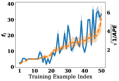
Figure 1: Average (standard error) of $f_{i},\text{APE}^{-0.5}$ over $20$ trials (sorted in increasing order of $\text{APE}^{-0.5}$ of $50$ training examples) with $\xi=1\text{e-}3$. Left (right) is logistic regression ($k$-nearest neighbors) using breast cancer (MNIST) dataset.

Table 1: Spearman coefficient between $f_{i}$ and $\text{APE}^{-0.5}$. Average (standard error) over $20$ independent trials. Higher is better.

$\xi$	breast cancer (logistic)	diabetes (ridge)
$1$e-$5$	6.89e-01 (1.41e-02)	5.49e-01 (2.24e-02)
$1$e-$4$	6.89e-01 (1.41e-02)	5.48e-01 (2.24e-02)
$1$e-$3$	6.78e-01 (1.50e-02)	5.53e-01 (2.20e-02)
$1$e-$2$	-1.94e-01 (2.59e-02)	5.67e-01 (2.32e-02)
$1$e-$1$	-1.47e-01 (2.60e-03)	5.00e-01 (2.55e-02)

Footnote 3 allows us to leverage the Chebyshev’s inequality to derive a fairness guarantee, through the minimum FS $\underline{f}\coloneqq\min_{i\in N}f_{i}$.

Proposition 1.

$\bm{\varphi}$ satisfy $(\epsilon_{1},\epsilon_{1}\xi,\delta)$-Shapley fairness where $\delta=1-(1-1/(\epsilon_{1}^{2}\underline{f}))^{n}$ if all $\varphi_{i}$’s are independent; otherwise  $\delta=n/(\epsilon_{1}^{2}\underline{f})$.

Proposition 1 (its proof is in Appendix C) formalises the effects of the variations in $\bm{\varphi}$ in satisfying probably approximate Shapley fairness where a larger minimum variation (i.e., $\underline{f}$) results in larger $\delta$, hence lower probability of $\bm{\varphi}$ satisfying the fairness axioms. To see whether $\varphi_{i}$’s are independent, it is equivalent to checking whether any permutation sampled is used for estimating multiple $\varphi_{i}$’s (proof in Appendix C).

The fidelity score, $f_{i}$, is sensitive to the number of sampled permutations and marginal contributions, $m_{i}$, as the variance of the SV estimator uses $m_{i}$ independent samples to produce $\mathbb{V}[\varphi_{i}]=\mathbb{V}[\sigma_{i}(\pi)]/m_{i}$. Therefore, we define an insensitive quantity, the invariability of $i$, $r_{i}$, as the FS with only one sample of $\pi$. Hence, $r_{i}\propto 1/\mathbb{V}[\sigma_{i}(\pi)]$ and here $\pi\sim U$. A higher $r_{i}$ implies that $i$-th marginal contribution is more invariable across different permutations. The fidelity score is product of the invariability and number of samples, i.e., $f_{i}=m_{i}r_{i}$, used in proving the following corollary.

Corollary 1.

Using the notations in Proposition 1, the minimum total budget $m=\sum_{i\in N}m_{i}$ needed to satisfy $(\epsilon_{1},\epsilon_{1}\xi,\delta)$-Shapley fairness is at most $\mathcal{O}(n\epsilon_{1}^{-2}(1-(1-\delta)^{1/n})^{-1})$ if $\varphi_{i}$’s are independent; and $\mathcal{O}(n^{2}\epsilon_{1}^{-2}\delta^{-1})$ o/w.

The budget complexity is an upper bound in a best/ideal case in the sense that our derivation (in Appendix C) uses $r_{i}$ which cannot be observed in practice. While it is not shown to be tight, our $\mathcal{O}(n)$ budget complexity for the independent scenario is linear in terms of the number of training examples, and the $\mathcal{O}(n^{2})$ budget complexity for the dependent scenario seems necessary for the $\mathcal{O}(n^{2})$ pairwise interactions between $\varphi_{i}$’s. Sec. 4 describes an estimation method that runs in the budget complexity upper bound given in Corollary 1.

4 Fairness via Greedy Active Estimation

To achieve probably approximate Shapley fairness with the lowest budget (number of samples) of marginal contribution evaluations, we propose a novel greedy active estimation (GAE) consisting of two core components - greedy selection and importance sampling. The first component efficiently split the training budget across examples while the second component influence and guide the sampling of permutations and reduce the variance $\mathbb{V}[\varphi_{i}]$ for each example $i$. In this section, we outline these components and show that they improve the minimum fidelity scores, $\underline{f}$. The details and full pseudo-code of the algorithm is given in Appendix A.

4.1 Greedy Selection using Pigou-Dalton

From Proposition 1, we can observe that a larger $\underline{f}$ decreases the probability of unfairness. Hence, to efficiently achieve probably approximate fairness, we should maximize $\underline{f}$ by improving the FS of the training example with the current lowest $f_{i}$. Our greedy method is outlined in Proposition 2 and formally proven in Appendix C.

Proposition 2 (Informal).

Given the constraint of evaluating a total of $m$ marginal contributions for all $j\in N$ to its predecessor set when the permutations are sampled from a fixed distribution $q$ (e.g., the uniform distribution). Then, the minimum FS $\underline{f}$ is maximised by (iteratively) greedily selecting and evaluating a marginal contribution of $i=\operatorname*{argmin}_{j\in N}f_{j}$, until $m$ is exhausted.

One direct implication is that greedy selection outperforms equally allocating the budget $m$ among all $N$ (i.e., $m_{i}=m/n$), which is used by existing methods (Sec. 2). Greedy selection will use a lower budget $m_{i}$ on a training example $i$ with higher invariability $r_{i}$ (lower variance in marginal contribution across permutations) to meet the same threshold $\underline{f}$. The budget will be mainly devoted to training examples with lower invariability and higher variance instead.

Moreover, improving $\underline{f}$ across all $i\in N$ is in line with the Pigou-Dalton principle (PDP) (Dalton 1920): Suppose we have two divisions of the budget that result in two sets of FSs denoted by $\bm{f},\bm{f}^{\prime}\in\mathbb{R}^{n}$ respectively. PDP prefers $\bm{f}$ to $\bm{f}^{\prime}$ if $\exists i,j\in N$ s.t., (a) $\forall k\in N\setminus\{i,j\},f_{k}=f_{k}^{\prime}$ and (b) $f_{i}+f_{j}=f_{i}^{\prime}+f_{j}^{\prime}$ and (c) $|f_{i}-f_{j}|<|f_{i}^{\prime}-f_{j}^{\prime}|$. PDP favors a division of the budget that leads to more equitable distribution of FSs. For SV estimation, it means we are approximately equally sure about all the estimates of the training examples, which can improve the effectiveness of identifying valuable training examples for active learning (Ghorbani, Zou, and Esteva 2021) (Fig. 3) or the potentially noisy/adversarial ones (Ghorbani and Zou 2019) (Fig. 5 in Appendix D). Theoretically, an inequitable distribution of FSs with some training examples with significantly lower $f_{i}$ will have a worse fairness guarantee (Proposition 1). We show that greedy selection satisfies PDP (Proposition 5 in Appendix C).

Remark. Although greedy selection maximizes the minimums FS, $\underline{f}$, it is not guaranteed to achieve approximate Shapley fairness with the highest probability as the probability bound in Proposition 1 is not tight (e.g., due to the application of union bound in derivation). Nevertheless, in Sec. 5, we empirically demonstrate that greedy selection indeed outperforms other existing methods in achieving probably approximate fairness. It is an appealing future direction to further improve the analysis and provide a tight bound for Proposition 1.

4.2 Active Permutation Selection via Importance Sampling

To improve the fidelity scores in Definition 3, our GAE method uses importance sampling to reduce $\mathbb{V}[\varphi_{i}]$ for every training example $i$ by setting $\varphi_{i}\coloneqq 1/m_{i}\sum_{t=1}^{m_{i}}\sigma_{i}(\pi^{t})/(q_{i}(\pi^{t})n!),\pi^{t}\sim q_{i}$. Here, $q_{i}$ is our proposal distribution over set of all permutations $\Pi$ that assigns probability $q_{i}(\pi)$ to permutation $\pi$. Following existing works (Castro et al. 2017; Ghorbani, Kim, and Zou 2020), we encode the assumption that any permutation, $\pi$, with the same cardinality for the predecessor set of $i$, $P_{i}^{\pi}$, should be assigned equal sampling probability. Hence $q_{i}(\pi)\propto q_{i}^{\prime}(|P_{i}^{\pi}|)$ where the function $q_{i}^{\prime}$ maps the predecessor’s cardinality to the sampling probability. We derive the optimal (but intractable) distribution $q_{i}^{*}(\pi)\propto q_{i}^{\prime*}(|P_{i}^{\pi}|)\propto(\mathbb{E}_{\pi\sim U(|P_{i}^{\pi}|)}[\sigma(\pi)^{2}])^{0.5}$ (proof in Appendix C) and approximate it with a “learnable” $q_{i}^{\prime}$. Specifically, we use a categorical distribution over the support $\{0,\ldots,n-1\}$ as $q_{i}^{\prime}$ and learn its parameters through maximum likelihood estimation (MLE) on tuples of predecessor set size and marginal contribution, with bootstrapping (i.e., sampling a small amount of permutations using MC, detailed in Appendix A). This active selection leads to both theoretical (Proposition 3) and empirical improvements (see Sec. 5), whilst ensuring $\mathbb{E}[\varphi_{i}]=\phi_{i}$ (Appendix B).

Proposition 3.

For a fixed budget $m$, denote the minimum FS achieved by greedy selection and active importance sampling, greedy selection only (with uniform sampling), and uniform MC sampling as $\underline{f}_{\text{GAE}},\underline{f}_{\text{greedy}}$ and $\underline{f}_{\text{MC}}$, respectively. Then, GAE outperforms the other methods as

$$\underline{f}_{\text{GAE}}\geq\underline{f}_{\text{greedy}}\geq\underline{f}_{\text{MC}}\ .$$

Furthermore, the minimum FSs $(\underline{f}_{\text{GAE}},\underline{f}_{\text{greedy}})$ are equal iff (a) $\forall i\in N,\mathbb{V}_{\pi\sim q^{*}_{i}}[\sigma_{i}(\pi)/(q_{i}^{*}(\pi)n!)]=\mathbb{V}[\sigma_{i}(\pi)]$ and the minimum FSs $(\underline{f}_{\text{greedy}},\underline{f}_{\text{MC}})$ are equal iff (b) every $i\in N$ has the same invariability w.r.t. $q_{i}^{*}$, ${r_{i,q_{i}^{*}}\coloneqq(|\phi_{i}|+\xi)^{2}/\mathbb{V}_{\pi\sim q^{*}_{i}}[\sigma_{i}(\pi)/(q_{i}^{*}(\pi)n!)]}$.

The proof is in Appendix C. In practice, equality conditions (a) and (b) are unlikely to hold. (a) only holds when our cardinality assumption ($i$-th marginal contribution to predecessor set of the same cardinality are similar) is wrong and unhelpful. A necessary but unrealistic condition for (b) is that for two data points $i,j$ with the same SV, their marginal contributions, i.e., the set $\{\sigma_{i}(\pi)|\pi\in\Pi\}$, must be equal.

Regularising importance sampling with uniform prior.

Proposition 3 requires the cardinality assumption so that the importance sampling approach (using $q_{i}^{\prime}$ which corresponds to a $q_{i}$) is effective by ensuring the derived $q_{i}$ is close to the theoretical optimal $q_{i}^{*}$. However, in practice, there are situations where using the uniform distribution $U$ performs better than $q_{i}$ obtained via learning $q_{i}^{\prime}$ using the cardinality assumption. First, if the marginal contributions on the same cardinality vary significantly (i.e., the cardinality assumption does not hold), then the approximation using $q_{i}$ is inaccurate. Second, if the marginal contributions over different cardinalities vary minimally, then importance sampling has little benefit as the marginal contributions are approximately equal. Interestingly, in both cases, using $U$ (treating all cardinalities uniformly) is the mitigation because it avoids using the incorrect inductive bias (i.e., the cardinality assumption).

Therefore, to incorporate $U$, we regularise the learning of $q_{i}^{\prime}$ with a uniform Dirichlet prior. Specifically, from the MLE parameters $\bm{w}\in\triangle(n)$ of $q_{i}^{\prime*},i\in N$ obtained via bootstrapping, and a uniform/flat Dirichet prior parameterised by $(\alpha+1)\mathbf{1}_{n},\alpha\geq 0$, we can obtain the maximum a posteriori (MAP) estimate as $n\bm{w}+(\alpha+1)\mathbf{1}_{n}$ (more details and derivations in Appendix B). With this, we unify the frequentist approach of learning $q_{i}^{\prime*}$’s parameters via purely MLE and the Bayesian approach of incorporating both likelihood and prior belief with $\alpha$ controlling how strong our prior belief is. Specifically, when $\alpha=0$, $q_{i}^{\prime}$ reduces to MLE and as $\alpha\rightarrow\infty$, $q_{i}^{\prime}$ tends to the uniform distribution over cardinality (due to the uniform Dirichlet prior) and thus the corresponding $q_{i}$ tends to $U$. In other words, if the cardinality assumption is satisfied (not satisfied), we expect the learned $q_{i}^{\prime}$ with a small (large) $\alpha$ to perform better (Sec. 5).

5 Experiments

We empirically verify that our proposed method can effectively mitigate the adverse situation described in introduction — the violation of the original symmetry axiom and its negative consequences (e.g., identical data are valued/priced very differently). We further compare GAE’s performance w.r.t. other axioms and PDP, and in different scenarios with real-world datasets against existing methods.

Specific problem scenarios and comparison baselines.

As mentioned in Sec. 2, our method is general, so we empirically investigate several specific problem scenarios in ML: P1. Data point valuation quantifies the relative effects of each training example in improving the learning performance (to remove noisy training examples or actively collect more valuable training examples) (Bian et al. 2022; Ghorbani, Kim, and Zou 2020; Ghorbani and Zou 2019; Jia et al. 2019, 2019; Kwon and Zou 2022). P2. Dataset valuation aims to provide value of a dataset among several datasets (e.g., in a data marketplace) (Agarwal, Dahleh, and Sarkar 2019; Ohrimenko, Tople, and Tschiatschek 2019; Xu et al. 2021b). P3. Agent valuation in the CML/FL setting determines the contributions of the agents to design their compensations (Sim et al. 2020; Song, Tong, and Wei 2019; Wang et al. 2020; Xu et al. 2021a). P4. Feature attribution studies the relative importance of features in a model’s predictions (Covert and Lee 2021; Lundberg and Lee 2017). We investigate P1. in detail in Sec. 5.1 and P2. P3. and P4. together in Sec. 5.2. We compare with the following estimation methods (as baselines): MC (Castro, Gómez, and Tejada 2009), stratified sampling (Castro et al. 2017; Maleki et al. 2013), multi-linear extension (Owen) (Okhrati and Lipani 2020; Owen 1972), Sobol sequences (Mitchell et al. 2022) and improved KernelSHAP (kernel) (Covert and Lee 2021).

5.1 Investigating A1-A3 and PDP within P1.

Settings.

We fit classifiers (e.g., logistic regression) on different datasets, use test accuracy as $v$ (Ghorbani and Zou 2019; Jia et al. 2019), and adopt Data Shapley (Ghorbani and Zou 2019, Proposition 2.1) as the SV definition. We randomly select $50$ training examples from a dataset and duplicate each once (i.e., a total of $n=100$ training examples). Following Sec. 3, we set $\xi=1\text{e-}3$. For bootstrapping (included for all baselines), we uniformly randomly select $20$ permutations and evaluate the marginal contributions for each $i$. We set a budget $m=2000$ for each baseline. As the true $\bm{\phi}$ are intractable for $n=100$, $\bm{\phi}$ is approximated via MC with significantly larger budget ($200$ bootstrapping permutations and $m=30000$, averaged over $10$ independent trials) as ground truth (in order to evaluate estimation errors) (Jia et al. 2019).

Effect of $\underline{f}$ on symmetry A2.

Proposition 1 implies a higher $\underline{f}$ leads to a better fairness guarantee. We specifically investigate the effect of $\underline{f}$ in mitigating mis-estimations of identical training examples and directly verify A2. We consider three evaluation metrics: lowest FS (i.e., $\underline{f}$); the proportion of duplicate pairs $i,i^{\prime}$ with estimates having a deviation larger than a threshold $t$, i.e., $|\varphi_{i}-\varphi_{i^{\prime}}|>t=\epsilon_{1}|\phi_{i}|+\xi\epsilon_{1}$ (as in A2); and the (log of) sum of the deviation ratio $\rho_{i,i^{\prime}}\coloneqq\max(\varphi_{i}/\varphi_{i^{\prime}},\varphi_{i^{\prime}}/\varphi_{i})$ over all $i,i^{\prime}$ pairs. In Fig. 2a,c, the $\underline{f}$ of our methods increases (improves) as the number of samples, $m$, increases. However, the $\underline{f}$ of all baseline methods are stagnated close to $0$. Thus, as expected, our method significantly outperforms the baselines in obtaining a high $\underline{f}$. As predicted by Proposition 1, this results in a lower probability and extent of fairness. As compared to baseline methods, our methods consistently have a lower proportion of identical examples that do not satisfy symmetry (A2) (Fig. 2b) and smaller deviation ratio of the estimated SV (Fig. 2d).

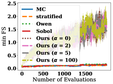
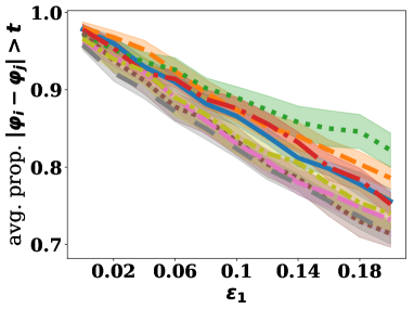
(a) $\underline{f}$ vs. $m$	(b) A2 violation ($\%$) vs. $\epsilon_{1}$
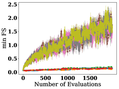
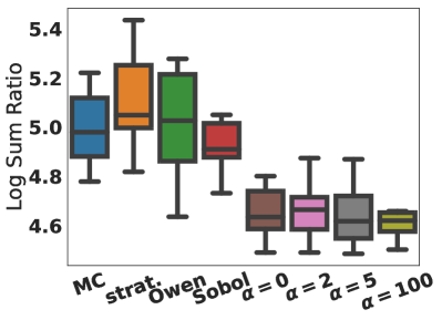
(c) $\underline{f}$ vs. $m$	(d) $\log\sum_{(i,i^{\prime})}\rho_{i,i^{\prime}}$

Figure 2: (a-b) and (c-d) plot results from using logistic regression on the synthetic Gaussian (Kwon and Zou 2022) and Covertype (Blackard 1998) datasets, respectively, using various baseline methods and ours. In (a,c), higher $\underline{f}$ is better while in (b,d), lower values are better. The intervals show the standard error of $10$ independent trials.

Verifying nullity A1 and Pigou Dalton Principle.

In practice, A1 is rarely applicable (i.e., $\forall\pi,\sigma_{i}(\pi)=0$), so we instead investigate a more likely scenario: $|\phi_{i}|$ is very small for some $i$, because the training example $i$ has a minimal impact during training (e.g., $i$ is redundant). We randomly draw $20$ training examples from the breast cancer dataset (Street 1995) to fit a support vector machine classifier (SVC). To verify A1, we standardize $\bm{\phi}$ and $\bm{\varphi}$ (i.e., $\bm{\phi}^{\top}\mathbf{1}_{n}=\bm{\varphi}^{\top}\mathbf{1}_{n}=1$) and calculate $\epsilon_{\text{abs}}\coloneqq\sum_{i:|\phi_{i}|\leq 0.01}|\varphi_{i}-\phi_{i}|$. As PDP is difficult to verify directly but it satisfies the Nash social welfare (NSW) (de Clippel 2010; Kaneko and Nakamura 1979), we use the (negative log of) NSW on standardized $\bm{f}$ (i.e., $\bm{f}^{\top}\mathbf{1}_{n}=n$) $\text{NL NSW}\coloneqq-\log\prod_{i\in N}f_{i}$ (lower indicates PDP is better satisfied). Tab. 2 shows our method obtains lowest estimation errors on (nearly) null training examples and satisfies PDP the best.

Table 2: Average (standard errors) of error and NL NSW over $10$ independent trials.

baselines	$\epsilon_{\text{abs}}$	NL NSW
MC	2.12e-02 (2.75e-03)	14.6 (5.12e-01)
Owen	6.33e-02 (4.04e-03)	18.2 (7.10e-01)
Sobol	6.28e-02 (5.64e-03)	11.6 (6.24e-01)
stratified	2.89e-02 (5.84e-03)	14.0 (7.46e-01)
kernel	6.44e-01 (1.15e-01)	21.4 (1.48)
Ours ($\alpha=0$)	1.72e-02 (3.50e-03)	2.24 (7.40e-01)
Ours ($\alpha=2$)	1.61e-02 (4.65e-03)	2.57 (5.28e-01)
Ours ($\alpha=5$)	1.42e-02 (4.00e-03)	2.55 (5.51e-01)
Ours ($\alpha=100$)	2.13e-02 (5.95e-03)	3.48 (5.61e-01)

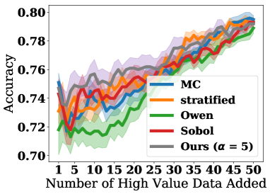
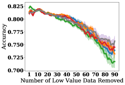
Figure 3: Accuracy of logistic regression adding (removing) training examples generated from Gaussian distribution with highest (lowest) $\varphi_{i}$ in left (right). Bootstrapping with $20$ permutations and $m=2000$. Average (standard errors in shaded color) over $10$ independent trials. KernelSHAP does not give clear trends in both plots because its estimates are not very accurate. Therefore we omit it here. A more detailed plot which involves KernelSHAP and other variants of our methods is provided in Appendix D.

Verifying approximate desirability A3.

For A3, we verify whether the valuable training examples have high $\varphi_{i}$ by adding (removing) training examples according to highest (lowest) $\varphi_{i}$ (Ghorbani and Zou 2019; Kwon and Zou 2022) (Fig. 3) and via noisy label detections (Jia et al. 2019) (Fig. 5 in Appendix D). Fig. 3 left (right) shows our method is effective in identifying the most (least) valuable training examples to add (remove).

5.2 Generalising to Other Scenarios

We examine the estimation accuracy, A3, and PDP within P2., P3. and P4.. For P2. we adopt robust volume SV (Xu et al. 2021b, Definition 3) (RVSV) and several real-world datasets for linear regression including used-car price prediction (use 2019) and credit card fraud detection (cre 2019) where $n$ data providers each owning a dataset (to estimate its RVSV). For P3. we consider (Sim et al. 2020, Equation 1) (CML) and hotel reviews sentiment prediction (hot 2016) and Uber-lyft rides price prediction (ube 2018); in addition, we also consider (Wang et al. 2020, Definition 1) (FL) using two image recognition tasks (MNIST (LeCun et al. 1990) and CIFAR-10 (Krizhevsky, Sutskever, and Hinton 2012)) and two natural language processing tasks (movie reviews (Pang and Lee 2005) and Stanford Sentiment Treebank-5 (Kim 2014)). We partition the original dataset into $n$ subsets, each owned by an agent $i$ in FL/CML and we estimate each agent’s contribution via the respective SV definitions. For P4. we follow (Lundberg and Lee 2017, Theorem 1) on several datasets including adult income (Kohavi and Becker 1996), iris (Fisher 1988), wine (Forina et al. 1991), and covertype (Blackard 1998) classification with different ML algorithms including $k$NN, logistic regression, SVM, and multi-layer perceptron (MLP). To ensure the experiments complete within reasonable time, we perform principal component analysis to obtain $7$ principal components/features for computing $\bm{\phi}$. For hyperparameters, since the largest $n$ among these scenarios is $7$, we set the budget $m=1000$ and the bootstrapping of $300$ evaluations (a total of $1300$ evaluations for each baseline). We set $\xi=1\text{e-}3$ and vary $\alpha\in\{0,2,5,100\}$ where $100$ simulates $\alpha\to\infty$. Additional experimental details (datasets, ML models etc) are in Appendix D.

Evaluation and results.

We examine the mean squared error (MSE) and mean absolute percentage error (MAPE) between $\bm{\varphi}$ and $\bm{\phi}$ for estimation accuracy, inversion counts $N_{\text{inv}}$ and errors $\epsilon_{\text{inv}}$ for A3 and NL NSW (defined previously) for PDP. The inversion count $N_{\text{inv}}\coloneqq\sum_{i\neq j\in N}\mathbb{1}(\phi_{i}>\phi_{j}\cap\varphi_{i}<\varphi_{j})+\mathbb{1}(\phi_{i}<\phi_{j}\cap\varphi_{i}>\varphi_{j})$ is the number of inverted pairings in $\bm{\varphi}$ while $\epsilon_{\text{inv}}\coloneqq\sum_{i\neq j\in N}|\phi_{i}-\phi_{j}-(\varphi_{i}-\varphi_{j})|$ is the sum of absolute errors (w.r.t. the true difference $\phi_{i}-\phi_{j}$). We present one set of average (and standard errors) over $5$ repeated trials for P2. P3. and P4. each in Tabs. 3, 4 and 5 (others in Appendix D). Overall, our method performs the best. While most methods perform competitively to ours w.r.t. MAPE, they are often worse (than ours) by an order of magnitude w.r.t. MSE. This is because our method explicitly addresses both the multiplicative and absolute errors (via $\xi=\epsilon_{2}/\epsilon_{1}$ in FS). Specifically, reducing absolute errors when $|\phi_{i}|$ is large (e.g., RVSV for P2. or (Sim et al. 2020, Equation 1) for P3. as both use the determinant of a large data matrix) is effective in reducing MSE. In our experiments, we find kernelSHAP underperforms others, which may be attributed to it having a larger (co-)variance, empirically verified in (Covert and Lee 2021).

Table 3: Evaluation of $\varphi_{i}$ within P2. using credit card dataset with $n=10$ data providers who each have a randomly sub-sampled dataset containing $100$ training examples (Xu et al. 2021b).

baselines	MAPE	MSE	$N_{\text{inv}}$	$\epsilon_{\text{inv}}$	NL NSW
MC	3.87e-02 (7.9e-03)	2.70e-03 (7.9e-04)	3.60 (1.33)	4.58 (0.82)	1.72e-02 (4.6e-03)
Owen	3.06e-02 (6.7e-03)	1.60e-03 (5.2e-04)	4.00 (1.41)	3.50 (0.76)	1.31e-02 (3.6e-03)
Sobol	6.75e-02 (3.4e-03)	9.62e-03 (1.5e-03)	4.80 (1.20)	7.97 (0.56)	7.46e-02 (1.3e-02)
stratified	4.46e-02 (8.3e-03)	3.30e-03 (8.3e-04)	4.40 (1.17)	5.17 (0.87)	1.72e-02 (5.9e-03)
kernel	0.10 (2.0e-02)	1.37e-02 (3.7e-03)	8.80 (2.15)	1.09e+01 (2.02)	3.64 (0.46)
Ours $(\alpha=0)$	0.10 (1.6e-02)	2.15e-02 (8.0e-03)	1.08e+01 (2.24)	1.18e+01 (1.85)	2.60 (0.88)
Ours $(\alpha=2)$	2.30e-02 (2.5e-03)	7.60e-04 (1.7e-04)	2.80 (1.02)	2.50 (0.29)	3.40e-04 (9.0e-05)
Ours $(\alpha=5)$	2.14e-02 (3.1e-03)	6.80e-04 (1.7e-04)	1.20 (0.49)	2.34 (0.31)	9.90e-04 (9.0e-05)
Ours $(\alpha=100)$	2.40e-02 (2.9e-03)	9.90e-04 (2.8e-04)	2.40 (0.75)	2.77 (0.42)	6.91e-03 (2.4e-03)

Table 4: Evaluation of $\varphi_{i}$ within P3. CML using hotel reviews dataset with $n=10$ agents who each have a randomly sub-sampled dataset containing $100$ training examples (Xu et al. 2021b).

baselines	MAPE	MSE	$N_{\text{inv}}$	$\epsilon_{\text{inv}}$	NL NSW
MC	3.53e-02 (6.0e-03)	2.00e-03 (7.0e-04)	1.32e+01 (2.94)	4.40 (0.83)	0.11 (3.0e-02)
Owen	3.06e-02 (1.3e-03)	1.23e-03 (1.7e-04)	1.00e+01 (1.41)	3.70 (0.24)	0.22 (5.0e-02)
Sobol	6.31e-02 (2.6e-03)	1.17e-02 (9.4e-04)	1.00e+01 (1.10)	8.54 (0.33)	0.28 (7.6e-02)
stratified	3.21e-02 (3.0e-03)	1.67e-03 (2.8e-04)	1.44e+01 (1.94)	4.10 (0.37)	0.20 (3.0e-02)
kernel	0.39 (5.7e-02)	0.23 (6.4e-02)	4.20e+01 (4.94)	4.89e+01 (7.24)	5.27 (1.34)
Ours $(\alpha=0)$	1.17e-02 (9.5e-04)	2.00e-04 (3.0e-05)	2.80 (0.49)	1.48 (0.12)	2.74e-03 (2.1e-04)
Ours $(\alpha=2)$	1.16e-02 (1.3e-03)	2.00e-04 (5.0e-05)	4.80 (1.96)	1.47 (0.18)	1.80e-02 (1.8e-03)
Ours $(\alpha=5)$	1.18e-02 (7.4e-04)	1.80e-04 (3.0e-05)	3.60 (1.33)	1.43 (0.10)	4.59e-02 (3.7e-03)
Ours $(\alpha=100)$	1.11e-02 (1.5e-03)	1.80e-04 (4.0e-05)	4.80 (1.62)	1.40 (0.18)	8.97e-02 (7.0e-03)

Table 5: Evaluation of $\varphi_{i}$ within P4. using the wine dataset on a randomly sampled subset of size $2000$ with $n=7$ principal features on a random forest classifier.

baselines	MAPE	MSE	$N_{\text{inv}}$	$\epsilon_{\text{inv}}$	NL NSW
MC	4.44e-02 (7.9e-03)	6.47e-03 (1.7e-03)	0.40 (0.40)	2.54 (0.41)	0.33 (3.1e-02)
Owen	9.88e-02 (1.0e-02)	1.77e-02 (3.4e-03)	1.20 (0.49)	4.51 (0.44)	0.44 (3.3e-02)
Sobol	0.24 (1.1e-02)	7.37e-02 (2.4e-03)	2.40 (0.40)	1.18e+01 (0.26)	1.32 (6.7e-02)
stratified	6.65e-02 (8.2e-03)	9.36e-03 (2.4e-03)	0 (0.0e+00)	2.62 (0.18)	0.34 (2.7e-02)
kernel	0.15 (3.2e-02)	1.56e-02 (4.1e-03)	3.60 (1.47)	6.08 (1.13)	1.05e+01 (0.20)
Ours $(\alpha=0)$	6.41e-02 (1.2e-02)	1.12e-02 (6.2e-03)	0.80 (0.49)	3.16 (0.75)	0.11 (2.7e-02)
Ours $(\alpha=2)$	3.65e-02 (5.0e-03)	2.49e-03 (7.7e-04)	0 (0.0e+00)	1.80 (0.26)	8.40e-02 (1.1e-02)
Ours $(\alpha=5)$	3.14e-02 (6.1e-03)	2.02e-03 (5.7e-04)	0 (0.0e+00)	1.54 (0.29)	0.16 (1.0e-02)
Ours $(\alpha=100)$	3.28e-02 (4.4e-03)	2.12e-03 (4.6e-04)	0.40 (0.40)	1.68 (0.23)	0.29 (1.3e-02)

6 Discussion and Conclusion

We propose probably approximate Shapley fairness via a re-axiomatisation of Shapley fairness and subsequently exploit an error-aware fidelity score (FS) to provide a fairness guarantee with a polynomial (in $n$) budget complexity. We identify that jointly considering multiplicative and absolute errors (via their ratio $\xi$) is crucial in the quality of the fairness guarantee (which existing works did not do). Through analysing the effect of $\xi$ on FS (used in our algorithm), we empirically find a suitable value for $\xi$. To achieve the fairness guarantee, we propose a novel greedy active estimation that integrates a greedy selection (which achieves a budget optimality) and active (permutation) selection via importance sampling. We identify that importance sampling can lead to poorer performance in practice as the necessary cardinality assumption may not be satisfied. To mitigate this, we describe a simple (via a single coefficient $\alpha$) regularisation using a uniform Dirichlet prior, that interestingly unifies the frequentist and Bayesian approaches (its effectiveness is empirically verified). For future work, it is appealing to explore whether there exists a biased estimator with much lower variance to provide a similar/better fairness guarantee with a competitive budget complexity.

Acknowledgements.

This research/project is supported by the National Research Foundation Singapore and DSO National Laboratories under the AI Singapore Programme (AISG Award No: AISG$2$-RP-$2020$-$018$). Xinyi Xu is also supported by the Institute for Infocomm Research of Agency for Science, Technology and Research (A*STAR)

Appendix A Algorithm Pseudo-code

Alg. 1 presents the pseudo-code for GAE. Greedy selection iteratively picks the $\varphi_{i}$ with the lowest $f_{i}$ to update its SV estimate using permutations obtained from active selection. This process repeats until the total budget $m$ is exhausted.

Algorithm 1 Greedy Active Estimator

procedure GAE($m^{\prime},m,N,q^{\prime},\xi$)

     # $m^{\prime}$: number of bootstrapping evaluations for each $\varphi_{i}$ ,

     # $m$: the total budget for all evaluations,

     # $N$: the set to be valued,

     # $q^{\prime}$: the proposal distribution that samples over the cardinalities $\{0,1,...,n-1\}$,

     # $\xi$: as in Footnote 3.

     Draw $m^{\prime}$ permutations $\pi_{t}\sim U(\Pi),\ t\in\{1,2,...,m^{\prime}\}$ $\triangleright$ For Bootstrapping

     Evaluate marginal contributions for each $i\in N$

     Estimate parameters of $q$ using the marginal contributions (details in Appendix B.4)

     Initialize all FSs using the marginal contributions (details in the paragraph below)

     $m_{i}\leftarrow m^{\prime},\ \forall i\in N$

     for $k\leftarrow 1$ to $m$ do

         $j\leftarrow\arg\min_{i\in N}\text{FS}(\varphi_{i},\xi)$ $\triangleright$ Greedy Selection

         $m_{j}\leftarrow m_{j}+1$

         $N^{\prime}\leftarrow N\setminus\{j\}$

         Draw cardinality sample $c\sim q^{\prime}$ $\triangleright$ Active Selection

         Draw a random permutation $\pi^{\prime}\sim U(\text{perm}(N^{\prime}))$

         $\pi_{m_{j}}\leftarrow\{\pi^{\prime}_{0},\pi^{\prime}_{1},...,\pi^{\prime}_{c-1},j,\pi^{\prime}_{c},..,\pi^{\prime}_{n-2}\}$

         Evaluate $\sigma_{j}(\pi_{m_{j}})$

         $w_{m_{j}}\leftarrow 1/(nq^{\prime}(c))$

         $\varphi_{j}\leftarrow(m_{j}-1)/m_{j}\times\varphi_{j}+w_{m_{j}}\sigma_{j}(\pi_{m_{j}})/m_{j}$

         $s_{j}^{2}\leftarrow 1/(m_{j}-1)\times\sum_{t=1}^{m_{j}}(w_{t}\sigma_{j}(\pi_{t})-\varphi_{j})^{2}$

         $f_{j}\leftarrow m_{j}\times(\varphi_{j}+\xi)^{2}/s_{j}^{2}$

     end for

     return $\varphi_{i}$ for all $i\in N$

end procedure

Bootstrapping the estimation of FS and proposal distribution $q$.

To mitigate the cold-start problem of obtaining accurate FS (and a good proposal distribution $q$), we draw $m^{\prime}$ bootstrapping permutations via MC (Efron and Tibshirani 1994) to obtain $m^{\prime}$ samples/marginal contributions for each $i$. Subsequently, for each $i$, the sample mean $\varphi_{i}=1/m^{\prime}\times\sum_{t=1}^{m^{\prime}}\sigma_{i}(\pi_{t})$ and sample variance $s_{i}^{2}=1/(m^{\prime}-1)\times\sum_{t=1}^{m^{\prime}}(\sigma_{i}(\pi_{t})-\varphi_{i})^{2}$ are then used to estimate the population mean $\mathbb{E}[\varphi_{i}]=\phi_{i}$ and population variance $\mathbb{E}[s_{i}^{2}]=\mathbb{V}[\sigma_{i}(\pi)]=m^{\prime}\mathbb{V}[\varphi_{i}]$. Both sample mean and sample variance are also used to estimate $f_{i}=\text{FS}(\varphi_{i},\xi)\approx m^{\prime}\times(\varphi_{i}+\xi)^{2}/s_{i}^{2}$ used in greedy selection. Additionally, the marginal contributions obtained during bootstrapping are used to estimate the parameters of the proposal distribution $q$ to improve its fit to the actual distribution of marginal contributions. While MC is used in bootstrapping, this choice is not restrictive and other approaches are also possible. For instance, if a good proposal distribution $q$ is known in advance (from prior knowledge), then $q$ can be applied both in bootstrapping and in active selection.

While our theoretical results (Propositions 2,3) require all marginal contributions used to estimate $f_{i}$ to be drawn from a fixed distribution $q$ (i.e., technically we should discard the marginal contributions obtained from bootstrapping if the permutations are drawn from $U$ which may be different from $q$), as $m\gg m^{\prime}$ in implementation, the $m^{\prime}$ samples from bootstrapping has a marginal impact, so we keep the marginal contributions (for estimating $\varphi_{i}$) as an implementation choice.

Appendix B Additional Analysis and Discussion

B.1 Equivalent Probabilistic Formulation of F1-F3 Using Conditional Events

1. Nullity: let $E_{F_{1}}$ be the (conditional) event that for any $i\in N$, conditioned on $(\forall\pi\in\Pi,\sigma_{i}(\pi)=0)$, then $\phi_{i}=0$.

2. Symmetry: let $E_{F_{2}}$ be the (conditional) event that for all $i\neq j\in N$, conditioned on $(\forall C\subseteq N\setminus\{i,j\},v(C\cup\{i\})=v(C\cup\{j\}))$, then $\phi_{i}=\phi_{j}$.

3. Strict desirability: let $E_{F_{3}}$ be the (conditional) event that for all $i\neq j\in N$, conditioned on $(\exists B\subseteq N\setminus\{i,j\},v(B\cup\{i\})>v(B\cup\{j\}))\wedge(\forall C\subseteq N\setminus\{i,j\},v(C\cup\{i\})\geq v(C\cup\{j\}))$, then $\phi_{i}>\phi_{j}$.

It can be verified that the probability of $E_{F_{1}}$-$E_{F_{3}}$ occurring is $1$, which is equivalent to the original formulation in the main text. Note that F1-F3 and A1-A3 are conditional events, so that the probability of the clause being satisfied is not relevant, instead the (conditional) probability of the implication, conditioned on the clause is satisfied, is what these axioms are designed to characterise and guarantee.

B.2 Variance Results for Some Existing Estimators

Continuing from the discussion in Sec. 3, we summarise the variance results of some existing estimators in Tab. 6.

Table 6: Variance results for some existing estimators. The variances for some estimators (e.g., Owen) are not available.

estimators	variance	remark	reference
MC	$\mathbb{V}_{\pi\sim U}[\sigma_{i}(\pi)]/m$	N.A.	(Castro, Gómez, and Tejada 2009, Proposition 3.1)
stratified	not available	a probabilistic error bound for each $\varphi_{i}$	(Maleki et al. 2013)
Owen	not available	N.A.	(Okhrati and Lipani 2020)
antithetic	$\mathbb{V}_{\pi\sim U}[\sigma_{i}(\pi)]/m\times[1+\text{Corr}(\sigma_{i}(X),\sigma_{i}(Y))]$	dependent on correlation	(Mitchell et al. 2022, Equation 4)
orthogonal	$1/m\sum_{l=1}^{n/k}\sum_{j,r=1}^{k}\text{Cov}(\sigma_{i}(\pi_{lj}),\sigma_{i}(\pi_{lr}))$	dependent on covariance	(Mitchell et al. 2022, Section 4.2)
Sobol	not available	N.A.	(Mitchell et al. 2022)
kernel	$M\Sigma_{\bm{\varphi}}M^{\top}$	covariance matrix	(Covert and Lee 2021, Equation 12).
Ours	$\mathbb{V}_{\pi\sim q_{i}}[\sigma_{i,q_{i}}(\pi)]/m$	dependent on the proposal distribution $q_{i}$	Equ. (4)

Stratified sampling has a probabilistic error bound (which additionally requires $\max_{C}\nu(C)$ and $\min_{C}\nu(C)$) for each $\varphi_{i}$ individually (Maleki et al. 2013, Equation 15): with probability at least $(1-\delta)^{n}$,

$$|\varphi_{i}-\phi_{i}|\leq\frac{d\sqrt{-\ln\frac{\delta}{2}}}{n\sqrt{m_{i}}}\left(\sum_{k=0}^{n-1}(k+1)^{\frac{2}{3}}\right)^{\frac{3}{2}},$$

where $d=2(\max v(C)/|C|-\min v(C)/|C|)$ and $m_{i}$ is the budget for evaluating $\varphi_{i}$. The contrast with our probably approximate fairness is that it does not consider the interaction between $\varphi_{i},\varphi_{j}$.

Antithetic is used in Owen and orthogonal is an extension of antithetic (Mitchell et al. 2022). $m$ refers to the number of sample permutations drawn. The variance of antithetic sampling estimator (Mitchell et al. 2022, Equation 4) depends on the correlation of a randomly sampled vector from a unit cube $X\sim U(0,1)^{n}$ and its complement $Y=\mathbf{1}_{n}-X$ element-wise. The orthogonal estimator (Mitchell et al. 2022, Equation 14) extends the antithetic sampling estimator, so its variance expression also extends that of the antithetic sampling estimator. Hence, to analyse the fairness guarantee, additional assumptions on the correlation or covariance are required.

Unfortunately, the variance results are not provided for the Sobol estimator (Mitchell et al. 2022, Algorithm 4) or Owen estimator (Okhrati and Lipani 2020, Algorithm 1) (compared in our experiments because they have empirically good performance (Mitchell et al. 2022; Okhrati and Lipani 2020)), so it is difficult to apply our proposed fairness framework to theoretically analyse their fairness.

Note that KernelSHAP is not a sampling-based estimator as it obtains $\bm{\varphi}$ by solving a regression. Hence, its variance result is a covariance matrix shown above with $M\coloneqq A^{-1}-(A^{-1}\mathbf{1}\mathbf{1}^{\top}A^{-1})/(\mathbf{1}^{\top}A^{-1}\mathbf{1})$ where $A_{ii}=1/2$ and

$$A_{ij,i\neq j}=\frac{1}{n(n-1)}\frac{\sum_{l=2}^{n-1}\frac{l-1}{n-l}}{\sum_{j=1}^{n-1}1/(l(n-l))}\ ,$$

and $\Sigma_{\bm{\varphi}}$ is the covariance matrix of (the vector) $\bm{\varphi}$.

From Tab. 6, it is appealing to provide the corresponding variance results for the existing unbiased estimators in order to analyse their fairness guarantee as in Definition 1. Furthermore, it is an interesting future direction to consider biased estimators with lower variance to achieve competitive fairness guarantees. For instance, a weighted importance sampling method for off-policy MC evaluation (Sutton and Barto 2018) leads to a biased estimator but empirically leads to faster convergence on some reinforcement learning tasks. More broadly, exploring how the variance vs. bias trade-off affects the fairness of an SV estimator is also an interesting direction to explore.

B.3 Limitations of MC

Firstly, MC is commonly adopted for each $i\in N$ separately (Castro, Gómez, and Tejada 2009; Maleki et al. 2013) (i.e., estimating $\varphi_{i}$ independently of others). As we have demonstrated in Fig. 1 and Fig. 4, $f_{i}\neq f_{j}$ in general even with the same number of permutation samples - some $\varphi_{i}$ observes larger variations than others due to large variation in their marginal contributions $\sigma_{i}(\pi)$. However, MC does not take this into consideration at all and as a result, cannot effectively optimise $\max\min_{i}f_{i}$ (optimising which provides the fairness guarantee as in Proposition 1 and Corollary 1)

Secondly, in MC, the permutations are selected uniformly randomly. However, it cannot guarantee that each $i$ receives permutations that are equally helpful in obtaining an accurate $\varphi_{i}$ (i.e., some permutations are more helpful in estimating $\varphi_{j}$ while some others more helpful for $\varphi_{i}$). For instance, the marginal contributions to subsets with smaller cardinality tend to be much larger in magnitude (Maleki et al. 2013; Ghorbani and Zou 2019; Kwon and Zou 2022). Intuitively, this echos diminishing returns where the performance improvement from adding a single training example to a small training set is more significant than that from adding the same training example to a large training set (Wang, Yang, and Jia 2021; Xu et al. 2021b). Without accounting for this, MC produces marginal contributions that have high variance.

The first limitation is addressed using greedy selection (Sec. 4.1). The second limitation is commonly tackled using importance sampling (Kloek, Kloek, and Van Dijk 1978): Permutations are drawn (randomly selected) from a proposal distribution $q_{i}(\pi)$ with densities according to $|\sigma_{i}(\pi)|$. Importance sampling can produce an unbiased estimator,

$$\phi_{i}=\mathbb{E}_{\pi\sim U(\pi)}[\sigma_{i}(\pi)]=\mathbb{E}_{\pi\sim q_{i}(\pi)}\left[\frac{U(\pi)\sigma_{i}(\pi)}{q_{i}(\pi)}\right]=\mathbb{E}_{\pi\sim q_{i}(\pi)}\left[\frac{\sigma_{i}(\pi)}{n!q_{i}(\pi)}\right],$$

where $U$ is a uniform distribution over all permutations $\Pi$. Theoretically, the optimal proposal distribution $q_{i}^{*}$ corresponds to when $\mathbb{V}[\sigma_{i}(\pi)/(q_{i}^{*}(\pi)n!)]$ is minimised. It implies the density is proportional to the magnitude of the true marginal contribution, i.e., $q_{i}^{*}\propto|\sigma_{i}(\pi)|$ (Yuan and Druzdzel 2007). However, $q_{i}^{*}$ is unattainable in practice without knowing all the marginal contributions.

B.4 Estimating the Parameters of the Categorical Distribution

It is natural to model the distribution of $|P_{i}^{\pi}|$ as a categorical distribution with a support as the different cardinalities $\{0,1,\ldots,n-1\}$. To obtain the parameters of the categorical distribution, one way is to directly estimate $\sqrt{\mathbb{E}_{\pi\sim U_{c}}[\sigma_{i}(\pi)^{2}]}$ (i.e., an MLE estimate as in Appendix C.3) where $U_{c}$ refers to the uniform distribution over all permutations of cardinality $c$: $\{\pi:\pi\in\Pi,|P_{i}^{\pi}|=c\}$. Another approach balances this estimation with a prior belief via a Dirichlet distribution (i.e., an MAP estimate) paramameterised by $\{\alpha_{0},\alpha_{1},\ldots,\alpha_{n-1}\}$, denoted as $\text{Dir}((\alpha_{0},\alpha_{1},\ldots,\alpha_{n-1}))$. The density of a $n$-dimensional probability vector $\{x_{0},x_{1},\ldots,x_{n-1}\}$ w.r.t. this Dirichlet distribution is

$$f(x_{0},x_{1},...,x_{n-1};\alpha_{0},\alpha_{1},...,\alpha_{n-1})=\frac{\Gamma\left(\sum_{k=0}^{n-1}\alpha_{k}\right)}{\prod_{k=0}^{n-1}\Gamma(\alpha_{k})}\prod_{k=0}^{n-1}x_{k}^{\alpha_{k}-1}\ .$$

We combine both approaches by setting an uninformative prior $\text{Dir}((\alpha+1)\bm{1}_{n})$ (i.e., $\alpha_{0}=\alpha_{1}=\ldots=\alpha_{n-1}=\alpha+1$) with a controllable strength via $\alpha$ (a larger $\alpha$ means we trust this prior more). We use the marginal contributions gathered from bootstrapping to update the Dirichlet distribution $\text{Dir}((\alpha+1)\bm{1}_{n})$. The goal is for the proposal distribution $q^{\prime}$ to approximate the optimal distribution well, specifically $q^{\prime*}$ (as shown in Equ. (5) later). To do so, we approximate $\mathbb{E}_{\pi\sim U_{c}}[\sigma_{i}(\pi)^{2}]$ which is a key component for $q^{\prime*}$.

Interpreting the MAP perspective. Let the MLE estimate be $\bm{w}$, the MAP estimate is then obtained by adding a constant term $\alpha$ to a scaled version of $\bm{w}$, denoted as $\bm{\tilde{w}}=n\bm{w}$. The scaling operation can be approximately viewed as drawing $n$ samples from $q^{\prime*}$, with $\tilde{w}_{c}$ falling into the $c$-th category. Therefore, $\bm{\tilde{w}}$ can be treated as coming from a categorical distribution $q^{\prime*}$, which combines with the Dirichlet prior to give an MAP estimate $\alpha+\tilde{w}_{c}$ for each category $c$.

Specifically, using the marginal contributions from bootstrapping, a probability simplex $\bm{w}$ (s.t. $\sum_{k=0}^{n-1}w_{k}=1$) is constructed where $w_{c}$ is proportional to the mean absolute marginal contribution with cardinality $c$, i.e., $w_{c}\propto 1/m_{i}\sum_{t=1}^{m_{i}}\sigma_{i}(\pi_{t})^{2}$ for $m_{i}$ samples drawn from $U_{c}$ to evaluate $\varphi_{i}$. Then the scaled $\tilde{\bm{w}}\leftarrow n\bm{w}$ is used to obtain the MAP estimate for the parameters $\bm{\theta}$ of the proposal distribution $q^{\prime}$ as $\theta_{c}=(\tilde{w}_{c}+\alpha)/\sum_{k=0}^{n-1}(\tilde{w}_{k}+\alpha)$. In particular, $\alpha=0$ recovers the MLE estimate. A detailed proof is given below.

Proof.

Notice that $\tilde{w}_{c}$ can be seen as the number of data belonging to the $c$-th category from $n$ observations. Further let $\bm{\theta}\sim\text{Dir}((\alpha+1)\bm{1}_{n})$. Then, the posterior distribution of $\bm{\theta}$ is

$$\text{Pr}(\bm{\theta}|\bm{\tilde{w}}) \propto\text{Pr}(\bm{\tilde{w}}|\bm{\theta})\text{Pr}(\bm{\theta}|\alpha)$$

$$\implies\log\text{Pr}(\bm{\theta}|\bm{\tilde{w}}) \propto\log\text{Pr}(\bm{\tilde{w}}|\bm{\theta})+\log\text{Pr}(\bm{\theta}|\alpha)\ .$$

Incorporate this equation with the constraint $\sum_{k=0}^{n-1}\theta_{k}=1$ to form the Lagrangian,

$$\mathcal{L}(\alpha,\bm{\theta}) =\log\text{Pr}(\bm{\tilde{w}}|\bm{\theta})+\log\text{Pr}(\bm{\theta}|\alpha)+\lambda\left(1-\sum_{k=0}^{n-1}\theta_{k}\right)$$

$$=\sum_{k=0}^{n-1}\tilde{w}_{k}\log\theta_{k}+\sum_{k=0}^{n-1}\alpha\log\theta_{k}+\lambda\left(1-\sum_{k=0}^{n-1}\theta_{k}\right).$$

Set its partial derivative w.r.t. $\theta_{c}$ to $0$ and solve for $\theta_{c}$, we get the MAP estimate for $\theta_{c}$

$$\theta_{c}^{\text{MAP}}=\operatorname*{argmax}_{\theta_{c}}\mathcal{L}(\alpha,\bm{\theta})=\frac{\tilde{w}_{c}+\alpha}{\sum_{k=0}^{n-1}(\tilde{w}_{k}+\alpha)}\ ,$$

which completes the proof. ∎

B.5 Greedy Active Estimator is Unbiased

We show that GAE produces unbiased estimates for all $\varphi_{i},\ i\in N$.

Proposition 4 (Unbiasedness of GAE).

Given a proposal distribution with support $\{0,1,2,...,n-1\}$, $\forall i,\mathbb{E}[\varphi_{i}]=\phi_{i}$ where each $\varphi_{i}$ is obtained from applying GAE.

Proof of Proposition 4.

Let $q$ be the sampling distribution that samples permutations according to our importance sampling method and proposal distribution. Since the support of our proposal distribution is the set of all cardinalities and every permutation of a fixed cardinality has equal (and therefore positive) probability of being selected, the support of $q$ is $\Pi$. Next, consider that for each $i\in N$, GAE produces an estimate $\varphi_{i}=\mathbb{E}_{\pi\sim q}[U(\pi)\sigma_{i}(\pi)/q(\pi)]$. Since the support of $q$ is $\Pi$, we have $\forall\pi\in\Pi,q(\pi)>0$. Hence $\varphi_{i}=\mathbb{E}_{\pi\sim q}[U(\pi)\sigma_{i}(\pi)/q(\pi)]=\mathbb{E}_{\pi\sim U}[\sigma_{i}(\pi)]=1/(n!)\sum_{\pi\in\Pi}\sigma_{i}(\pi)=\phi_{i}$ by Equ. (1). ∎

Appendix C Proofs and Derivations

C.1 Proof of Proposition 1

To aid the proofs of the guarantee of Axioms A1-A3, we introduce the following intermediate fidelity axiom:

1. Closeness: For any $i\in N$, the estimated SV $\varphi_{i}$, can deviate from the true SV $\phi_{i}$ by a relative error $\epsilon_{1}$ and an absolute error $\epsilon_{2}$:

   $$|\phi_{i}-\varphi_{i}|\leq\epsilon_{1}|\phi_{i}|+\epsilon_{2}\ .$$ (2)

Lemma 1.

Denote $\underline{f}\coloneqq\min_{i\in N}f_{i}$, then the fidelity axiom  A0 with error parameters $\epsilon_{1},\epsilon_{2}$ in (2) is satisfied for any $i\in N$ w.p. $\geq 1-1/(\epsilon_{1}^{2}f_{i})\geq 1-1/(\epsilon_{1}^{2}\underline{f})$.

Proof of Lemma 1.

From (2),

$$\begin{split}\text{Pr}[|\phi_{i}-\varphi_{i}|\leq\epsilon_{1}|\phi_{i}|+\epsilon_{2}]&=1-\text{Pr}[|\phi_{i}-\varphi_{i}|>\epsilon_{1}|\phi_{i}|+\epsilon_{2}]\\ &\geq 1-\frac{\mathbb{V}[\varphi_{i}]}{(\epsilon_{1}^{2}|\phi_{i}|+\epsilon_{2})^{2}}\\ &=1-\frac{1}{\epsilon_{1}^{2}f_{i}}\\ &\geq 1-\frac{1}{\epsilon_{1}^{2}\underline{f}}\ .\end{split}$$

The first inequality is by Chebyshev’s inequality and the last inequality is by $\underline{f}=\min_{i\in N}f_{i}$. ∎

Proof of Proposition 1.

By Chebyshev’s inequality, A0 in Equ. (2) holds for some $i\in N$ w.p. $\geq 1-1/(\epsilon_{1}^{2}f_{i})$ (Lemma 1). Let A0 hold for all $i\in N$ simultaneously, w.p. $\geq 1-\delta_{A0}$ (the expression for $\delta_{A0}$ is derived later).

The case for A1 is straightforward by substituting $\phi_{i}=0$ into (2).

For A2 and A3, first the apply triangle inequality,

$$|\phi_{i}-\varphi_{i}-\phi_{j}+\varphi_{j}|\leq|\phi_{i}-\varphi_{i}|+|-\phi_{j}+\varphi_{j}|\ ,$$

then apply (2),

$$|\phi_{i}-\varphi_{i}-\phi_{j}+\varphi_{j}|\leq\epsilon_{1}(|\phi_{i}|+|\phi_{j}|)+2\epsilon_{2}\ .$$ (3)

For A2, substitute $\phi_{i}=\phi_{j}$ into (3),

$$|-\varphi_{i}+\varphi_{j}|\leq\epsilon_{1}(|\phi_{i}|+|\phi_{j}|)+2\epsilon_{2}\ .$$

For A3, substitute $\delta_{ij}\coloneqq\phi_{i}-\phi_{j}$ and $\hat{\delta}_{ij}\coloneqq\varphi_{i}-\varphi_{j}$ into (3),

$$|\delta_{ij}-\hat{\delta}_{ij}|\leq\epsilon_{1}(|\phi_{i}|+|\phi_{j}|)+2\epsilon_{2}\ .$$

Hence, A1-A3 are satisfied (for all $i\in N$ or $i,j\in N$) if A0 is holds for all $i\in N$ simultaneously.

To derive $\delta_{A0}$, consider two cases: i) all $\varphi_{i}$’s are independent, then $\delta_{A0}\leq(1-1/(\epsilon_{1}^{2}\underline{f}))^{n}$.

Otherwise, ii) $\delta_{A0}\leq n/(\epsilon_{1}^{2}\underline{f})$ (by the union bound of the complement):

$$\text{Pr}[\forall i\in N,\text{A0 holds}] =1-\text{Pr}[\exists i\in N,\text{A0 does not hold}]$$

$$\geq 1-\sum_{i}\text{Pr}[\text{A0 does not hold for }i]$$

$$\geq 1-n/(\epsilon_{1}^{2}\underline{f})$$

where the first inequality is by the union bound and the second inequality is by Lemma 1. Lastly, substituting Definition 1 completes the proof. ∎

Remark 1.

If all $\varphi_{i}$’s are independent, a tighter bound for fairness (shown above) is $p\coloneqq\prod_{i}(1-1/(\epsilon_{1}^{2}f_{i}))$ (w.p. $\geq 1-p$ the properties are satisfied w.r.t. $\epsilon_{1},\epsilon_{2}$). Therefore, to improve fairness, we can instead improve its lower bound $p$. Specifically, we consider which $i$ to evaluate one additional budget so as to maximise the improvement in $p$. Let $f_{i}$ and $f_{i}^{\prime}$ denote the fidelity score of $i$ when it has received $m_{i}$ budget and after being evaluated one additional budget (i.e., $m_{i}+1$ based on the $\varphi_{i}$ of the $m_{i}$ budget), respectively.

The (multiplicative) improvement $\Delta_{p}$ of $p$ is defined as $\Delta_{p}\coloneqq p^{\prime}/p$ where $p^{\prime}$ refers to the fairness bound after receiving one additional evaluation. Then,

$$\Delta_{p}=\frac{p^{\prime}}{p}=\frac{1-\frac{1}{\epsilon_{1}^{2}f_{i}^{\prime}}}{1-\frac{1}{\epsilon_{1}^{2}f_{i}}}=\frac{1-\frac{1}{\epsilon_{1}^{2}(m_{i}+1)r_{i}}}{1-\frac{1}{\epsilon_{1}^{2}m_{i}r_{i}}}=\frac{\epsilon_{1}^{2}r_{i}-\frac{1}{m_{i}+1}}{\epsilon_{1}^{2}r_{i}-\frac{1}{m_{i}}}\ .$$

Observe that to maximise $\Delta_{p}$ (equivalently to improve $p$) which depends on $r_{i},m_{i}$, we should select $i$ s.t., $r_{i},m_{i}$ maximise $\Delta_{p}$ each time. This observation gives rise to a modified version of the Greedy Active Estimator (GAE): Instead of evaluating $\operatorname*{argmin}_{i}f_{i}$, the modified algorithm evaluates $\operatorname*{argmax}_{i}\Delta_{p}(r_{i},m_{i})$. However, one practical limitation is that $\epsilon_{1}$ has to be specified, which implies the improved bound (i.e., better $p$) is specific to some fixed $\epsilon_{1}$ and may not generalise to other values of $\epsilon_{1}$. Note that GAE circumvents this limitation since $\underline{f}$ does not require a specified $\epsilon_{1}$.

Moreover, through analysing the partial derivatives of $\Delta_{p}$ w.r.t $r_{i},m_{i}$, we believe finding $i$ via $\operatorname*{argmin}f_{i}$ is a good surrogate for $\operatorname*{argmax}\Delta_{p}(r_{i},m_{i})$ without having to pre-specify $\epsilon_{1}$. Note that

$$\Delta_{p}=1+\frac{1}{\epsilon_{1}^{2}r_{i}+1}\left(\frac{1}{m_{i}+1}+\frac{\epsilon_{1}^{2}r_{i}}{1-\epsilon_{1}^{2}r_{i}m_{i}}\right)\ ,$$

which gives the partial derivative w.r.t. $r_{i}$ and $m_{i}$ as

$$\frac{\partial\Delta_{p}}{\partial r_{i}} =-\frac{\epsilon_{1}^{2}m_{i}}{(\epsilon_{1}^{2}r_{i}m_{i})^{2}(m_{i}+1)}\ ,$$

$$\frac{\partial\Delta_{p}}{\partial m_{i}} =\frac{1}{\epsilon_{1}^{2}r_{i}+1}\left(\frac{\epsilon_{1}^{4}r_{i}^{2}}{(1-\epsilon_{1}^{2}r_{i}m_{i})^{2}}-\frac{1}{(m_{i}+1)^{2}}\right)\ .$$

Observe that $\frac{\partial\Delta_{p}}{\partial r_{i}}<0$ always holds, while $\frac{\partial\Delta_{p}}{\partial m_{i}}<0$ when $\epsilon_{1}^{2}<\frac{1}{r_{i}(2m_{i}+1)}$. Therefore, if $\epsilon_{1}$ is (sufficiently) small, then $\Delta_{p}$ is larger for smaller $r_{i},m_{i}$ (i.e., select $i\in N$ with small $r_{i},m_{i}$). As a surrogate, $\underline{f}=\min_{i}f_{i}=\min_{i}r_{i}m_{i}$ can capture this relationship and is thus the design choice in our algorithm (i.e., greedy selection).

Remark 2.

Proof of independence of $\varphi_{i},\varphi_{j}$. Express $\varphi_{i}=f_{i}(\mathcal{X}_{i})$ and $\varphi_{j}=f_{j}(\mathcal{X}_{j})$, where $f_{i},f_{j}:2^{\Pi}\rightarrow\mathbb{R}$ are two deterministic functions that map (a set of) permutations to a real value (i.e., the respective SV estimate) and $\mathcal{X}_{i}$ is the random variable denoting the set of randomly sampled permutations for calculating $\varphi_{i}\leftarrow f_{i}(\mathcal{X}_{i})$ (elaborating lines 36-37). Note that we assume all marginal contributions $\sigma_{i}(\pi),\sigma_{j}(\pi),\forall\pi\in\Pi$ are fixed (though unknown), given a well defined problem. It can be seen that $\varphi_{i},\varphi_{j}$ are independent if $\mathcal{X}_{i},\mathcal{X}_{j}$ are independent.

C.2 Proof of Corollary 1

Proof of Corollary 1.

We prove the corollary by considering two cases:

i) All $\varphi_{i}$’s are independent. From $\delta=1-(1-1/(\epsilon_{1}^{2}\underline{f}))^{n}$, solve for $\underline{f}$,

$$\underline{f}\geq\frac{1}{\epsilon_{1}^{2}(1-(1-\delta)^{1/n})}\ ,$$

and since $r_{i}m_{i}\geq\underline{f}$

$$m_{i}\geq\frac{1}{\epsilon_{1}^{2}(1-(1-\delta)^{1/n})r_{i}}\ ,$$

which implies the total budget

$$m =\sum_{i\in N}m_{i}$$

$$\geq\sum_{i\in N}\frac{1}{\epsilon_{1}^{2}(1-(1-\delta)^{1/n})r_{i}}$$

$$=\epsilon_{1}^{-2}(1-(1-\delta)^{1/n})^{-1}\sum_{i\in N}\frac{1}{r_{i}}$$

$$\geq\epsilon_{1}^{-2}(1-(1-\delta)^{1/n})^{-1}\frac{n}{\max_{i\in N}r_{i}}$$

$$=\mathcal{O}(n\epsilon_{1}^{-2}(1-(1-\delta)^{1/n})^{-1})\ .$$

ii) Otherwise, $\varphi_{i}$’s may be dependent of each other. From $\delta=n/(\epsilon_{1}^{2}\underline{f})$, solve for $\underline{f}$,

$$\underline{f}\geq\frac{n}{\epsilon_{1}^{2}\delta}\ ,$$

and since $r_{i}m_{i}\geq\underline{f}$

$$m_{i}\geq\frac{n}{\epsilon_{1}^{2}\delta r_{i}}\ ,$$

which implies the total budget

$$m =\sum_{i}m_{i}$$

$$\geq\sum_{i}\frac{n}{\epsilon_{1}^{2}\delta r_{i}}$$

$$=n\delta^{-1}\epsilon_{1}^{-2}\sum_{i\in N}\frac{1}{r_{i}}$$

$$\geq n\delta^{-1}\epsilon_{1}^{-2}\frac{n}{\max_{i\in N}r_{i}}$$

$$=\mathcal{O}(n^{2}\epsilon_{1}^{-2}\delta^{-1})\ .$$

∎

From the above derivations, it can be implied that any estimator which keeps track of $\underline{f}$ and stops soon long as the target $\underline{f}$ is achieved is able to obtain the upper bound budget complexity. As our proposed Greedy Active Estimator (GAE) iteratively updates $\underline{f}$, by terminating it when the current evaluation improves $\underline{f}$ to the desired value, GAE runs in the budget upper bound.

C.3 Importance Sampling for Variance Reduction

Following (Castro et al. 2017; Kwon and Zou 2022), we restrict the sampling probability of a permutation $\pi$, $q_{i}(\pi)$, to depend on the cardinality of the predecessor set, $|P_{i}^{\pi}|$. Precisely, let $q_{i}^{\prime}$ be a discrete distribution defined on the support $\{0,1,2,\ldots,n-1\}$ that maps the cardinality $c$ of the predecessor set to the probability that any permutation of cardinality $c$ is drawn. The sampling probability $q_{i}(\pi)=q_{i}^{\prime}(|P_{i}^{\pi}|)/(n-1)!$ for a specific permutation $\pi$ because there are other $(n-1)!$ equally likely permutations $\pi^{\prime}$ where $|P^{\pi}_{i}|=|P^{\pi^{\prime}}_{i}|$ (i.e., the position of $i$ in permutations $\pi$ and $\pi^{\prime}$ is the same).

We minimise the variance of the importance sampling estimator to derive the optimal importance sampling distributions $q_{i}^{\prime*}(c)$ (over the support $\{0,1,\ldots,n-1\}$) and $q_{i}^{*}(\pi)$ (over the support $\Pi$). Let $\tilde{\mathbb{V}}_{q_{i}}[\sigma_{i}(\pi)]\coloneqq\mathbb{V}_{\pi\sim q_{i}}[\sigma_{i}(\pi)/(q_{i}(\pi)n!)]$ denotes the probability adjusted variance of $\sigma_{i}(\pi)$ (Elvira and Martino 2022), using the sampling distribution $q_{i}$ supported on $\Pi$; The variance of marginal contribution $\sigma_{i}(\pi)$ of $i$ w.r.t. a permutation $\pi$ sampled from a proposal distribution $q_{i}$ is

$$\tilde{\mathbb{V}}_{q_{i}}[\sigma_{i}(\pi)] =\sum_{\pi\in\Pi}\left(\frac{(\sigma_{i}(\pi)/n!-\phi_{i}q_{i}(\pi))^{2}}{q_{i}(\pi)}\right)$$ (4)

$$=\sum_{\pi\in\Pi}\frac{1}{n!}\left(\frac{(\sigma_{i}(\pi)/n!-\phi_{i}q_{i}(\pi))^{2}}{q_{i}(\pi)}\times n!\right).$$

Using the Lagrange multiplier and differentiating Equ. (8) to minimise the above variance, we will show that the following optimal distributions can be obtained:

$$q_{i}^{\prime*}(c)=\sqrt{\mathbb{E}_{\pi\sim U_{c}}[\sigma_{i}(\pi)^{2}]}\Big{/}\left(\sum_{k=0}^{n-1}\sqrt{\mathbb{E}_{\pi\sim U_{k}}[\sigma_{i}(\pi)^{2}]}\right)\ ,$$ (5)

and therefore, by substituting $q_{i}(\pi)=q_{i}^{\prime}(|P_{i}^{\pi}|)/(n-1)!$, we get the optimal sampling distribution of permutation $q_{i}^{*}(\pi)$

$$q^{*}_{i}(\pi)=\frac{q^{\prime*}_{i}(|P^{\pi}_{i}|)}{(n-1)!}\ .$$ (6)

The optimality of $q_{i}^{\prime*}(c)$ and hence $q_{i}^{*}(\pi)$ can be proved as follows. Denote $\mathbb{E}_{U_{c}}=\mathbb{E}_{\pi\sim U_{c}}$ where $U_{c}$ is defined as in Appendix B.4 to represent uniform distribution of permutations with a fixed cardinality. Further denote $\sigma=\sigma_{i}(\pi)$. Then, the variance can be rewritten as the average of $\mathbb{E}_{U_{c}}$ over all cardinalities $c\in\{0,1,2,...,n-1\}$

$$\tilde{\mathbb{V}}_{q_{i}}[\sigma_{i}(\pi)] =\sum_{\pi\in\Pi}\frac{1}{n!}\left(\frac{(\sigma_{i}(\pi)/n!-\phi_{i}q_{i}(\pi))^{2}}{q_{i}(\pi)}\times n!\right)$$ (7)

$$=\sum_{c=0}^{n-1}\sum_{\pi\in\{\pi:|P_{i}^{\pi}|=c\}}\frac{1}{n!}\left(\frac{(\sigma_{i}(\pi)/n!-\phi_{i}q_{i}(\pi))^{2}}{q_{i}(\pi)}\times n!\right)$$

$$=\sum_{c=0}^{n-1}\sum_{\pi\in\{\pi:|P_{i}^{\pi}|=c\}}\frac{1}{n!}\left(\frac{(\sigma_{i}(\pi)/n!-\phi_{i}q_{i}^{\prime}(c)/(n-1)!)^{2}}{q_{i}^{\prime}(c)/(n-1)!}\times n!\right)$$

$$=\sum_{c=0}^{n-1}\sum_{\pi\in\{\pi:|P_{i}^{\pi}|=c\}}\frac{1}{n!}\left(\frac{(\sigma_{i}(\pi)-n\phi_{i}q_{i}^{\prime}(c))^{2}}{n!nq_{i}^{\prime}(c)}\times n!\right)$$

$$=\frac{1}{n}\sum_{c=0}^{n-1}\sum_{\pi\in\{\pi:|P_{i}^{\pi}|=c\}}\frac{1}{(n-1)!}\left(\frac{(\sigma_{i}(\pi)-n\phi_{i}q_{i}^{\prime}(c))^{2}}{n!nq_{i}^{\prime}(c)}\times n!\right)$$

$$=\frac{1}{n}\sum_{c=0}^{n-1}\mathbb{E}_{U_{c}}\left[\frac{(\sigma-n\phi_{i}q^{\prime*}_{i}(c))^{2}}{n!nq^{\prime}_{i}(c)}\times n!\right]$$

$$=\frac{1}{n}\sum_{c=0}^{n-1}n!\times\left(\frac{\mathbb{E}_{U_{c}}[\sigma^{2}]}{n!nq^{\prime}_{i}(c)}-\frac{2\mathbb{E}_{U_{c}}[\sigma]\phi_{i}}{n!}+\frac{n\phi_{i}^{2}q^{\prime}_{i}(c)}{n!}\right)$$

$$=\frac{1}{n}\sum_{c=0}^{n-1}\left(\frac{\mathbb{E}_{U_{c}}[\sigma^{2}]}{nq^{\prime}_{i}(c)}-2\mathbb{E}_{U_{c}}[\sigma]\phi_{i}+n\phi_{i}^{2}q^{\prime}_{i}(c)\right)$$

$$=\frac{1}{n}\sum_{c=0}^{n-1}\left(\frac{\mathbb{E}_{U_{c}}[\sigma^{2}]}{nq^{\prime}_{i}(c)}-2\mathbb{E}_{U_{c}}[\sigma]\phi_{i}\right)+\phi_{i}^{2}\ .$$

For a fixed $c$, minimise the summands in Equ. (7) over the choice of $q_{i}^{\prime}(c)$ s.t. $\sum_{c=0}^{n-1}q_{i}^{\prime}(c)=1$, which can be reformulated as the following Lagrangian after discarding the constant term $n\phi_{i}^{2}$,

$$\begin{split}\mathcal{G}&=\frac{1}{n}\sum_{c=0}^{n-1}\left(\frac{\mathbb{E}_{U_{c}}[\sigma^{2}]}{nq^{\prime}_{i}(c)}-2\mathbb{E}_{U_{c}}[\sigma]\phi_{i}\right)-\lambda\left(1-\sum_{c=0}^{n-1}q_{i}^{\prime}(c)\right).\end{split}$$

Set its partial derivative w.r.t. $q_{i}^{\prime}(c)$ to $0$,

$$\begin{split}\frac{\partial\mathcal{G}}{\partial q_{i}^{\prime}(c)}&=(-\frac{\mathbb{E}_{U_{c}}[\sigma^{2}]}{n^{2}q_{i}^{\prime}(c)^{2}})+\lambda=0\\ q_{i}^{\prime*}(c)&=\frac{\sqrt{\mathbb{E}_{U_{c}}[\sigma^{2}]}}{\sqrt{n^{2}\lambda}}\propto\sqrt{\mathbb{E}_{U_{c}}[\sigma^{2}]}\ .\end{split}$$

The direct proportionality uses the fact that $q_{i}^{\prime*}(c)$ is independent of $n$ and $\lambda$. To satisfy $\sum_{c=0}^{n-1}q_{i}^{\prime*}(c)=1$, we standardise all $q_{i}^{\prime*}(c)$ and obtain Equ. (5), which completes the proof.

Now, we prove that importance sampling by cardinality strictly outperforms MC. Denote $S=\sum_{k=0}^{n-1}\sqrt{\mathbb{E}_{k}[\sigma^{2}]}$. Plug Equ. (5) back into Equ. (7),

$$\begin{split}\tilde{\mathbb{V}}_{q_{i}^{*}}[\sigma_{i}(\pi)]&=\frac{1}{n}\sum_{c=0}^{n-1}\left(\frac{\sqrt{\mathbb{E}_{U_{c}}[\sigma^{2}]}S}{n}-2\mathbb{E}_{U_{c}}[\sigma]\phi_{i}+\frac{n\phi_{i}^{2}\sqrt{\mathbb{E}_{U_{c}}[\sigma^{2}]}}{S}\right).\end{split}$$

For MC, we take advantage of the linearity of expectation and evaluate its variance by breaking variance into strata of different cardinalities. Substitute $q_{i}(\pi)$ with $1/n!$,

$$\begin{split}\tilde{\mathbb{V}}_{U}[\sigma_{i}(\pi)]&=\frac{1}{n}\sum_{c=0}^{n-1}\mathbb{E}_{U_{c}}\left[\frac{(\sigma/n!-\phi_{i}/n!)^{2}}{(1/n!)^{2}}\right]\\ &=\frac{1}{n}\sum_{c=0}^{n-1}\mathbb{E}_{U_{c}}\left[(\sigma-\phi_{i})^{2}\right]\\ &=\frac{1}{n}\sum_{c=0}^{n-1}\left(\mathbb{E}_{U_{c}}[\sigma^{2}]-2\phi_{i}\mathbb{E}_{U_{c}}[\sigma]+\phi_{i}^{2}\right).\end{split}$$

The two variances are compared via a subtraction,

$$\tilde{\mathbb{V}}_{q_{i}^{*}}[\sigma_{i}(\pi)]-\tilde{\mathbb{V}}_{U}[\sigma_{i}(\pi)] =\frac{\phi_{i}^{2}}{n}\sum_{c=0}^{n-1}\left(\frac{n\sqrt{\mathbb{E}_{U_{c}}[\sigma^{2}]}}{S}-1\right)+\sum_{c=0}^{n-1}\frac{1}{n}\left(\frac{\sqrt{\mathbb{E}_{U_{c}}[\sigma^{2}]}S}{n}-\mathbb{E}_{U_{c}}[\sigma^{2}]\right)$$

$$=0+\sum_{c=0}^{n-1}\frac{1}{n}\left(\frac{\sqrt{\mathbb{E}_{U_{c}}[\sigma^{2}]}S}{n}-\mathbb{E}_{U_{c}}[\sigma^{2}]\right)$$

$$=\frac{1}{n}\left(\frac{S^{2}}{n}-\sum_{c=0}^{n-1}\mathbb{E}_{U_{c}}[\sigma^{2}]\right).$$

Next, note that $S^{2}=(\sum_{k=0}^{n-1}\sqrt{\mathbb{E}_{k}[\sigma^{2}]})^{2}\leq n\sum_{k=0}^{n-1}\mathbb{E}_{k}[\sigma^{2}]$ by the Cauchy Schwarz inequality. Then,

$$\tilde{\mathbb{V}}_{q_{i}^{*}}[\sigma_{i}(\pi)]-\tilde{\mathbb{V}}_{U}[\sigma_{i}(\pi)] =\frac{1}{n}\left(\frac{S^{2}}{n}-\sum_{c=0}^{n-1}\mathbb{E}_{U_{c}}[\sigma^{2}]\right)\leq 0$$ (8)

$$\implies\tilde{\mathbb{V}}_{q_{i}^{*}}[\sigma_{i}(\pi)] \leq\tilde{\mathbb{V}}_{U}[\sigma_{i}(\pi)]$$

where equality holds if and only if the equality condition for the Cauchy Schwarz inequality holds, i.e., $\mathbb{E}_{U_{0}}[\sigma^{2}]=\mathbb{E}_{U_{1}}[\sigma^{2}]=...=\mathbb{E}_{U_{n-1}}[\sigma^{2}]$.

C.4 Proof of Proposition 2

Before proving Proposition 2, we first provide a formal version of the proposition.

Proposition (formal Budget Optimality of Greedy Selection).

For a fixed budget $m$, denote $\underline{f}_{A}$ as the minimum FS obtained by estimation algorithm $A$. Let $\mathcal{A}_{q}$ be the set of all sampling-based estimation methods (defined in Sec. 2) that sample permutations from a fixed distribution $q$. Then, greedy selection (this is, iteratively selecting $i=\operatorname*{argmin}_{j\in N}f_{j}$) with the same underlying distribution $q$ achieves the optimal minimum FS, $\underline{f}_{\text{GS},q}$. In other words, $\underline{f}_{\text{GS},q}=\max_{A\in\mathcal{A}_{q}}\underline{f}_{A}$.

In short, Proposition 2 suggests that if we break up a sampling-based estimation method into two parts: 1) choosing a $\varphi_{i}$ to evaluate, and 2) sampling a permutation for it, then greedy selection chooses the $\varphi_{i}$’s in such a way that the resulting minimum fidelity score is the highest, given a fixed underlying sampling distribution.

Proof of Proposition 2.

First recall the invariability of $\varphi_{i}$

$$r_{i}\coloneqq\frac{(|\phi_{i}|+\xi)^{2}}{\mathbb{V}[\sigma_{i}(\pi)]}=\frac{f_{i}}{m_{i}}$$

where $m_{i}$ is the budget $i$ receives. Since the sampling distribution $q$ is fixed, $r_{i}$ is fixed and does not vary with $m_{i}$. Suppose the optimal $\underline{f}$ is $f^{*}$. To achieve $f^{*}$, every $i\in N$ with an initial FS (after bootstrapping) $f_{i}^{(0)}<f^{*}$ must receive at least $e_{i}=\lceil(f^{*}-f_{i}^{(0)})/r_{i}\rceil$ budget to ensure that its resulting FS reaches/exceeds $f^{*}$. Now, suppose greedy selection has made $e_{j}$ evaluations for some $j\in N$. If every $i\in N\setminus\{j\}$ has FS greater than $f^{*}$, then $f^{*}$ is achieved and the algorithm terminates. Otherwise it evaluates some $i$ with FS smaller than $f^{*}$. As such, each $i\in N$ receives exactly $e_{i}$ evaluations, the minimum budget needed to achieve $f^{*}$. Equivalently, with the same total budget, greedy selection achieves the highest $\underline{f}$ among all sampling-based algorithms with the underlying distribution $q$. ∎

C.5 Proof of Proposition 3

Proof of Proposition 3.

We first derive $\underline{f}_{\text{greedy}}$ and $\underline{f}_{\text{MC}}$. For MC, as each $i\in N$ receives $m/n$ evaluations,

$$\underline{f}_{\text{MC}}=\min f_{i}(\varphi_{i})=\min_{i\in N}\frac{m}{n}r_{i}=\frac{m\min_{i\in N}r_{i}}{n}\ .$$ (9)

For greedy selection, to simplify analysis, we made a mild assumption that each $r_{i}$ is relatively small as compared to the number of samples $m$ so that with a careful allocation of $m_{i}$ samples to $i$, it is possible to achieve $r_{i}m_{i}=r_{j}m_{j}$ for all $i,j\in N$. Then,

$$\forall i,j\in N,r_{i}m_{i} =r_{j}m_{j}$$ (10)

$$\sum_{i\in N}m_{i} =m$$

$$\Longrightarrow m_{i} =\frac{m}{r_{i}\sum_{j\in N}1/r_{j}}$$

$$\Longrightarrow\underline{f}_{\text{greedy}} =m_{i}r_{i}=\frac{m}{\sum_{j\in N}1/r_{j}}\ .$$

With Equ. (9) and Equ. (10), $\underline{f}_{\text{GAE}}$ can be related to $\underline{f}_{\text{greedy}}$. First, from $\tilde{\mathbb{V}}_{q_{i}^{*}}[\sigma_{i}(\pi)]\leq\tilde{\mathbb{V}}_{U}[\sigma_{i}(\pi)]$ in Equ. (8), so for any $i\in N$,

$$\frac{1}{r_{i,U}}-\frac{1}{r_{i,q_{i}^{*}}} =\frac{\tilde{\mathbb{V}}_{U}[\sigma_{i}(\pi)]}{(|\phi_{i}|+\xi)^{2}}-\frac{\tilde{\mathbb{V}}_{q_{i}^{*}}[\sigma_{i}(\pi)]}{(|\phi_{i}|+\xi)^{2}}$$

$$=\frac{\tilde{\mathbb{V}}_{U}[\sigma_{i}(\pi)]-\tilde{\mathbb{V}}_{q_{i}^{*}}[\sigma_{i}(\pi)]}{(|\phi_{i}|+\xi)^{2}}\geq 0\ ,$$

which implies $\forall i\in N,1/r_{i,U}\geq 1/r_{i,q_{i}^{*}}$ and hence $\sum_{j\in N}1/r_{j,U}\geq\sum_{j\in N}1/r_{j,q_{j}^{*}}$. Then,

$$\frac{\underline{f}_{\text{GAE}}}{\underline{f}_{\text{greedy}}} =\frac{\frac{m}{\sum_{j\in N}1/r_{j,q_{j}^{*}}}}{\frac{m}{\sum_{j\in N}1/r_{j,U}}}$$

$$=\frac{\sum_{j\in N}1/r_{j,U}}{\sum_{j\in N}1/r_{j,q_{j}^{*}}}$$

$$\geq 1$$

where equality is taken if and only if $\forall i\in N,\ r_{i,U}=r_{i,q_{i}^{*}}$, which completes the first part of the proof.

For the second part of the proof, with Equ. (9) and Equ. (10), similarly divde $\underline{f}_{\text{greedy}}$ by $\underline{f}_{\text{MC}}$,

$$\frac{\underline{f}_{\text{greedy}}}{\underline{f}_{\text{MC}}} =\frac{\frac{m}{\sum_{j\in N}1/r_{j}}}{\frac{m\min_{i\in N}r_{i}}{n}}$$ (11)

$$=\frac{n}{\min_{i\in N}r_{i}\sum_{j\in N}1/r_{j}}$$

$$=\frac{n}{\sum_{j\in N}\frac{\min_{i\in N}r_{i}}{r_{j}}}$$

$$\geq\frac{n}{\sum_{j\in N}\frac{r_{j}}{r_{j}}}$$

$$=\frac{n}{n}=1$$

where the inequality becomes equality if and only if $\forall i,j\in N,\ r_{i}=r_{j}$.

∎

C.6 Proof of Proposition 5

Proposition 5.

Given fixed $r_{i}$ for each $i$, greedy selection satisfies PDP.

Proof of Proposition 5.

We show greedy selection satisfies PDP. To see this, let an alternative estimation process produce final fidelity scores $\bm{f}^{\prime}$ satisfying $k^{*}$ such that $\forall k\in N\setminus\{i,j\},f_{k}^{\prime}=f_{k}$ and $f_{i}^{\prime}+f_{j}^{\prime}=f_{i}+f_{j}$. Without loss of generality, let $f_{i}<f_{j}$. Further let the initial fidelity score of each $i\in N$ be $f_{i}^{(0)}$ and consider two cases: 1) $f_{i}^{(0)}=f_{i}$. In this case, greedy selection makes no evaluations on $i$. Hence $f_{i}^{\prime}\geq f_{i}$ since making evaluations on $i$ can only improve its fidelity score. Thus $|f_{i}-f_{j}|=f_{j}-f_{i}=f_{i}^{\prime}+f_{j}^{\prime}-2f_{i}\leq f_{i}^{\prime}+f_{j}^{\prime}-2f_{i}^{\prime}=f_{i}^{\prime}-f_{j}^{\prime}\leq|f_{i}^{\prime}-f_{j}^{\prime}|$; 2) $f_{i}^{(0)}<f_{i}$. In this case greedy selection makes evaluations on $i$. However, notice that greedy selection stops improving $f_{i}$ once $f_{i}\geq k^{*}$. Hence, for any $f_{i}^{\prime}$ that satisfies $k^{*}$, it must be the case that $f_{i}^{\prime}\geq f_{i}$. As such, reuse the argument for case 1, we have $|f_{i}-f_{j}|<|f_{i}^{\prime}-f_{j}^{\prime}|$. Therefore, under no circumstance is an alternative estimation process preferred over greedy selection, namely, greedy selection satisfies PDP. ∎

To give an intuitive illustration of PDP, consider a dataset (of $3$ training examples) evaluated using two estimators $p_{1}$ and $p_{2}$ that lead to FSs of $(25,5,5)$ and $(20,10,5)$ respectively. Though they both have $\underline{f}=5$ (thus the same fairness guarantee by Corollary 1), $p_{1}$ is less fair (than $p_{2}$) in its allocation of estimation budget as $p_{1}$ overly focuses on the $1$st training example (instead of the other two). Note PDP prefers $(20,10,5)$ to $(25,5,5)$, as desired. Because PDP is w.r.t. the estimation method and not individual $\varphi_{i}$, it can be considered a characteristic of the estimation and thus not included in the fairness guarantee (Definition 1).

Appendix D Additional Experimental Results

D.1 Dataset License

Covertype (Blackard 1998): Apache License 2.0; Breast cancer (Street 1995): Apache License 2.0; Iris (Fisher 1988): Apache License 2.0; Adult income (Kohavi and Becker 1996): Apache License 2.0; Wine (Forina et al. 1991): Apache License 2.0; Diabetes (Efron et al. 2004): : Attribution-NonCommercial 4.0 International (CC BY-NC 4.0); MNIST (Deng 2012): Creative Commons Attribution-Share Alike 3.0; CIFAR-10 (Krizhevsky, Sutskever, and Hinton 2012): The MIT License (MIT); Movie reviews (Pang and Lee 2005): BSD 3-Clause ”New” or ”Revised” License; Stanford Sentiment Treebank (Kim 2014): BSD 3-Clause ”New” or ”Revised” License; Credit Card (cre 2019): Database Contents License (DbCL); Uber & Lyft (ube 2018): CC0 1.0 Universal (CC0 1.0); Used Car (use 2019): CC0 1.0 Universal (CC0 1.0); Hotel Reviews (hot 2016): Attribution-NonCommercial 4.0 International (CC BY-NC 4.0).

D.2 Computational Resources

For all our experiments requiring only CPUs, we use a server with 2 $\times$ Intel Xeon Silver 4116 ($2.1$Ghz) as the computing resource. For experiments requiring GPUs (i.e., in P3. we train one model for one agent for multiple agents), we utilise a server with Intel(R) Xeon(R) Gold 6226R CPU @$2.90$GHz and four NVIDIA GeForce RTX 3080’s.

D.3 Additional Experimental Settings

Utility of the null set.

As there is no standard way of defining the utility of the null set (i.e., $v(\emptyset)$), in all our experiments using test accuracy as the utility function, we initialise the ML learner by randomly picking a coalition $C_{0}$ comprising of two entries, one from each class outside the training set, and set $v(\emptyset)$ as the utility value of $C_{0}$. For each coalition $C$, we define $v(C)$ as the utility value of $C\cup C_{0}$. This way, we make sure that at least one entry from each class is present to train the classifier. We do the same for all experiments using negative MSE as the utility function, but picking only one entry outside the training set as we only require one entry to train a regressor. For experiments on other specific scenarios, $\nu(\emptyset)$ follows the respective references.

Approximation of $f_{i}$.

In Footnote 3, $f_{i}$ depends on $\phi_{i}$ and $\mathbb{V}[\varphi_{i}]$ which are intractable to obtain in practice. Therefore, suppose that we have made $m$ evaluations, $f_{i}$ is approximated by first estimating $\phi_{i}\approx\varphi_{i}=1/m\sum_{t=1}^{m}\sigma_{i}(\pi_{t})$ and $\mathbb{V}_{\pi\sim q}[\varphi_{i}]\approx s^{2}/m=1/[m(m-1)]\sum_{t=1}^{m}(w_{t}\sigma_{i}(\pi_{t})-\varphi_{i})^{2}$, where $w_{t}=1/(q(\pi_{t})n!)$ (for sampling over cardinalities, we use $w_{t}=1/(q^{\prime}(|P_{i}^{\pi}|)n)$). Then $f_{i}\approx m\times\varphi_{i}/s^{2}$.

Additional details on other SV estimation baselines

We compare against Sobol sequences out of the four proposed methods in (Mitchell et al. 2022) because it is the most computationally efficient and is reported to have the best/competitive performance.

Additional details for P2..

We partition a dataset (e.g., used-car price prediction) to $n=8$ agents/data providers, so that each data provider exclusively owns data (price information) of cars from a particular manufacturer (e.g., Audi, Ford, etc). For the two datasets considered for P2., we set $n=8$ or $n=10$, which is larger than $n=3$ in the original work (Xu et al. 2021b).

While P2. provides a dataset valuation function based on the theoretical framework of linear regression, our experiments (following (Xu et al. 2021b)) explore beyond linear regression and consider applications of DNNs For instance, we perform additional feature pre-processing such as the GloVe word embeddings (Pennington, Socher, and Manning 2014) to create a $8$-dimensional pre-processed feature from a bidirectional long short-term memory model for hotel reviews dataset. Subsequently, the linear regression/RVSV is w.r.t. the pre-processed $8$-dimensional feature.

Additional details for P3..

In the CML experiments, the uber lyft ride price (hotel review sentiment) prediction dataset presents a $12$ ($8$)-dimensional regression task. Therefore, the experiment setting follows (Sim et al. 2020) to calculate the mutual information of the $12$ or $8$ parameters of a Bayesian linear regression using a Gaussian process (with a radial basis kernel whose lengthscale parameter is automatically learnt). In the FL experiments, the dataset partition, used ML models and training hyperparameters such as batch size, learning rate etc, follow (Xu et al. 2021a).

D.4 Additional Results for $f_{i}$ Against APE

Under the same experiment setting as Fig. 1, additional experimental results for $f_{i}$ Against APE using different dataset and ML algorithm combinations are in Fig. 4.

We randomly select a subset of $50$ training examples from the Covertype dataset to train using a logistic regression classifier and set test accuracy as the utility function $v$ (Ghorbani and Zou 2019). Since the exact SV (for comparison in APE) is intractable, we approximate it (as the ground truth in APE) using the MC estimate (denoted by $\bar{\phi}$), i.e., an average of $5000$ marginal contributions w.r.t. uniformly randomly selected permutations. As $f_{i}$ is also intractable, we approximate it using $f_{i}\approx 50\times\bar{\phi}/s^{2}$ where $s^{2}=\left((\sum_{t=1}^{50}\sigma_{i}(\pi_{t})^{2})-(\sum_{t=1}^{50}\sigma_{i}(\pi_{t}))^{2}/50\right)/49$. We evaluate each training example with $50$ permutations drawn from simple random sampling and plot $f_{i}$ against $\sqrt{1/\text{APE}}$ in Fig. 1 which shows a higher $f_{i}$ corresponds to a lower APE, as expected. Note the ‘ground truth’ is approximated with MC estimates with $100$ times the budget than in the actual estimation (Jia et al. 2019; Xu et al. 2021a).

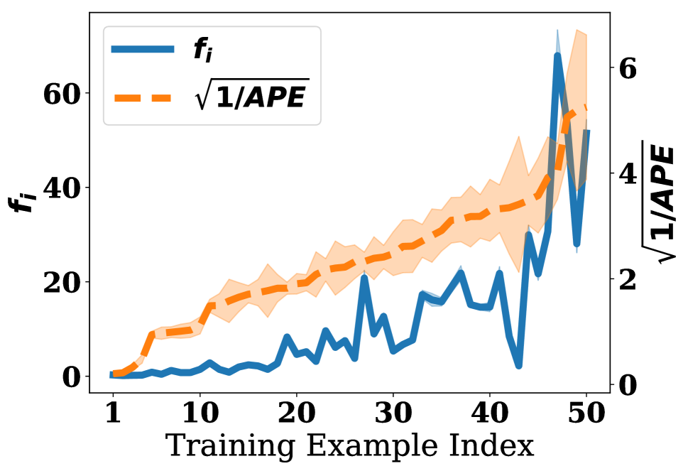
(a) Covertype Logistic: $(0.701\pm 0.019)$

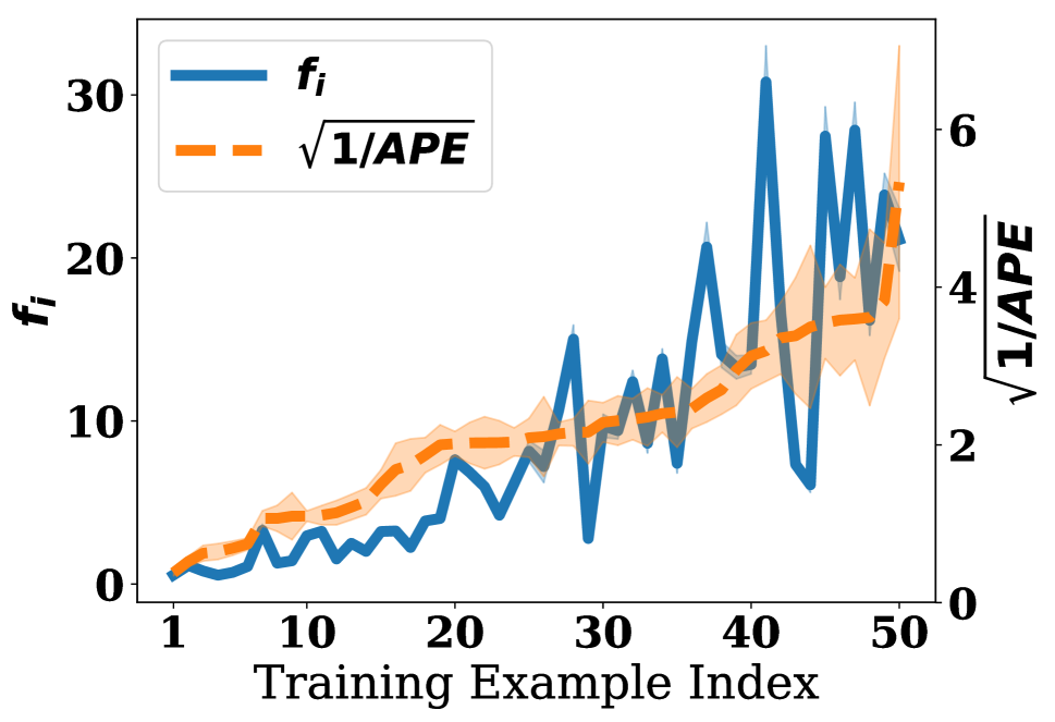
(b) Beast Cancer Logistic: $(0.678\pm 0.015)$

(c) MNIST Logistic: $(0.580\pm 0.020)$

(d) Synthetic Gaussian Logistic: $(0.536\pm 0.029)$

(e) Covertype $k$NN: $(0.713\pm 0.015)$

(f) Breast Cancer $k$NN: $(0.409\pm 0.024)$

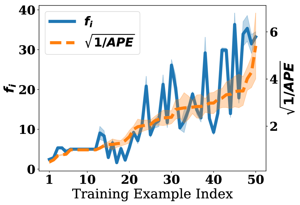
(g) MNIST $k$NN: $(0.689\pm 0.012)$

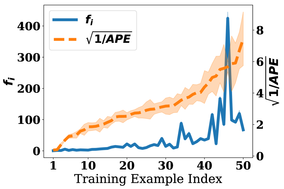
(h) Synthetic Gaussian $k$NN: $(0.681\pm 0.013)$

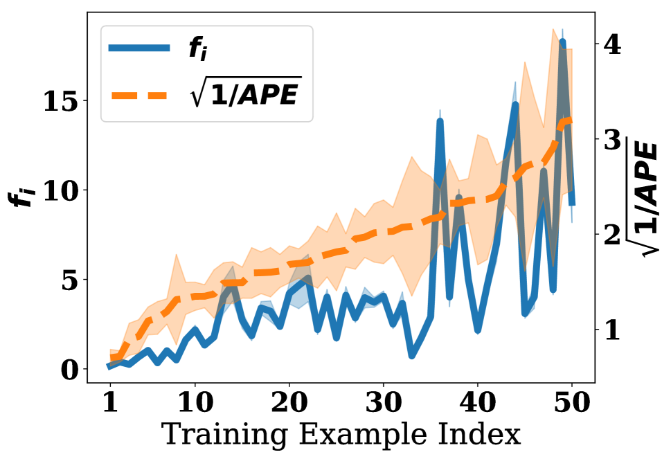
(i) Covertype SVC: $(0.529\pm 0.031)$

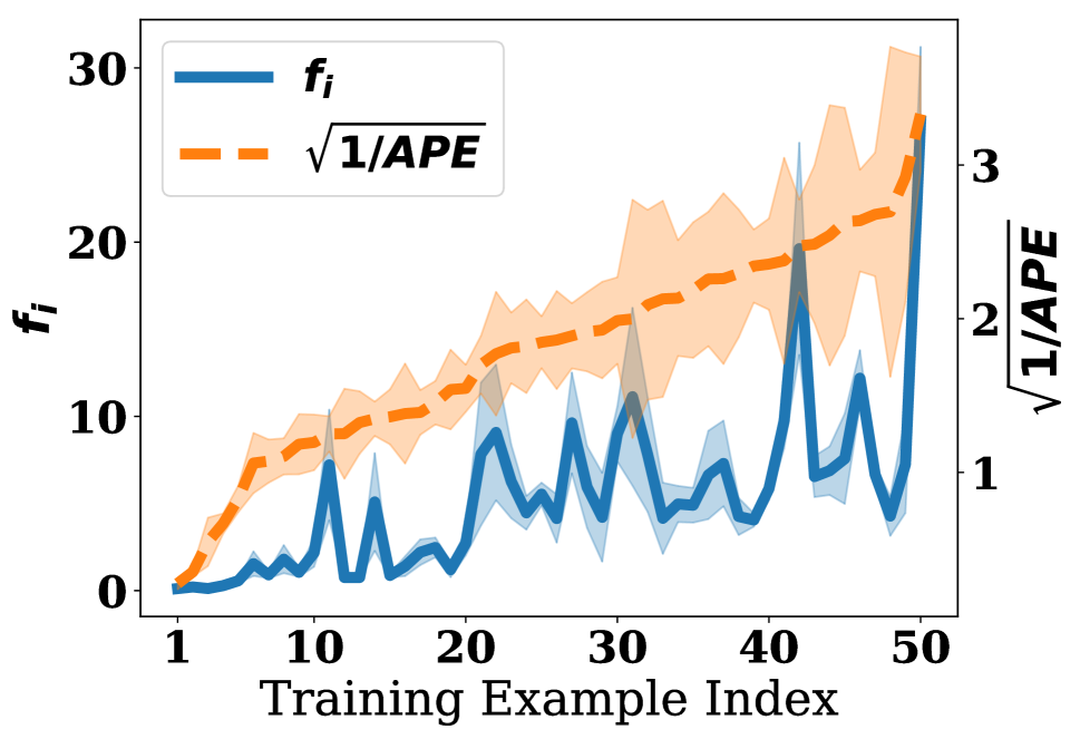
(j) Breast Cancer SVC: $(0.498\pm 0.021)$

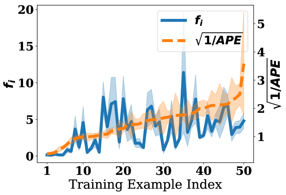
(k) MNIST SVC: $(0.444\pm 0.017)$

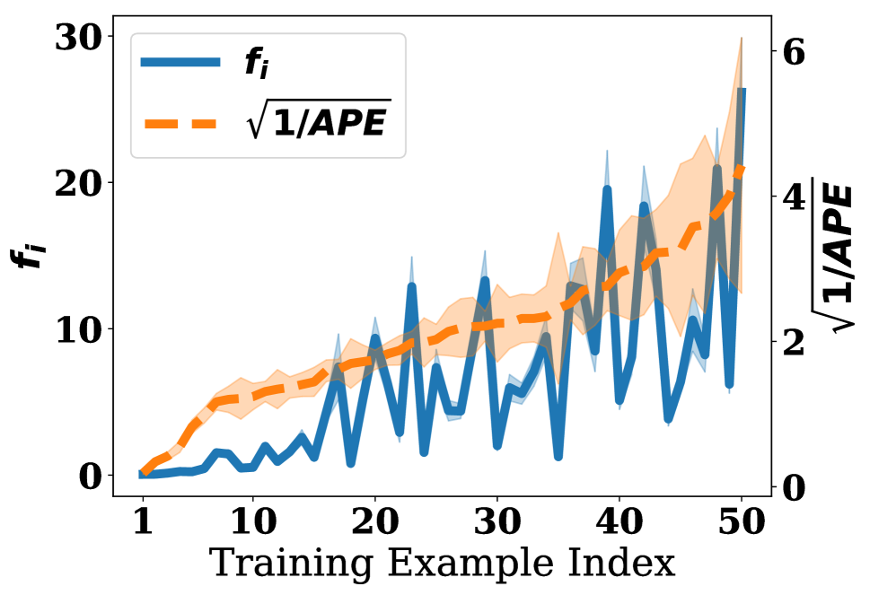
(l) Synthetic Gaussian SVC: $(0.583\pm 0.025)$

Figure 4: The plot of $f_{i}$ vs. $\sqrt{1/\text{APE}}$ for $50$ training examples over $20$ repeated trials. Caption of each plot shows the dataset and learner, followed by the average and standard error of the Spearman Rank coefficient.

D.5 Additional Experimental Results

Under the same experimental setting in Sec. 5.2 and the additional settings described above where applicable, additional experimental results are presented: average (standard errors) over $5$ independent trials for dataset valuation (Tab. 7), CML (Tab. 8), FL (Tabs. 9 and 16), and feature attribution (Tabs. 17 and 19). For all metrics, lower is better.

Table 7: Evaluation of $\varphi_{i}$ within P2. using used car price with $n=8$ data providers who each have a randomly sub-sampled dataset containing $100$ training examples (Xu et al. 2021b).

baselines	MAPE	MSE	$N_{\text{inv}}$	$\epsilon_{\text{inv}}$	NL NSW
MC	2.23e-02 (2.0e-03)	9.00e-04 (1.8e-04)	0.80 (0.49)	1.66 (0.14)	2.66e-02 (5.1e-03)
Owen	1.67e-02 (2.8e-03)	5.30e-04 (1.6e-04)	0.80 (0.80)	1.31 (0.21)	2.70e-02 (2.6e-03)
Sobol	5.59e-02 (2.3e-03)	4.35e-03 (4.1e-04)	2.80 (0.49)	4.12 (0.18)	0.12 (1.1e-03)
stratified	2.52e-02 (3.3e-03)	1.14e-03 (2.7e-04)	1.20 (0.80)	1.97 (0.25)	4.20e-02 (6.2e-03)
kernel	0.11 (1.5e-02)	1.57e-02 (4.7e-03)	5.20 (0.49)	7.22 (0.88)	3.10 (0.26)
Ours (a=0)	2.67e-02 (3.9e-03)	1.08e-03 (2.4e-04)	1.20 (0.80)	1.96 (0.28)	0.23 (4.9e-02)
Ours (a=2)	1.42e-02 (1.6e-03)	3.10e-04 (6.0e-05)	0.80 (0.49)	1.07 (0.12)	3.78e-03 (1.1e-03)
Ours (a=5)	1.19e-02 (8.5e-04)	2.50e-04 (6.0e-05)	0.80 (0.49)	0.90 (7.7e-02)	8.40e-03 (2.3e-03)
Ours (a=100)	1.55e-02 (2.7e-03)	4.70e-04 (2.0e-04)	0.40 (0.40)	1.09 (0.17)	1.79e-02 (4.3e-03)

Table 8: Evaluation of $\varphi_{i}$ within P3. CML uber lyft ride price dataset with $n=10$ agents who each have a randomly sub-sampled dataset containing $50$ training examples (Xu et al. 2021b).

baselines	MAPE	MSE	$N_{\text{inv}}$	$\epsilon_{\text{inv}}$	NL NSW
MC	4.91e-02 (9.8e-03)	3.80e-03 (1.3e-03)	1.88e+01 (3.88)	6.24 (1.19)	1.66e-02 (6.6e-03)
Owen	3.76e-02 (7.8e-03)	2.32e-03 (7.6e-04)	1.28e+01 (3.01)	4.76 (0.98)	1.37e-02 (4.2e-03)
Sobol	7.72e-02 (3.6e-03)	1.02e-02 (6.2e-04)	3.44e+01 (2.48)	9.92 (0.55)	6.96e-02 (3.3e-03)
stratified	6.28e-02 (1.1e-02)	5.83e-03 (1.5e-03)	1.80e+01 (2.28)	7.76 (1.31)	3.19e-02 (1.1e-02)
kernel	7.37e-02 (4.1e-03)	8.57e-03 (1.1e-03)	2.84e+01 (2.93)	9.70 (0.50)	0.86 (0.17)
Ours (a=0)	0.15 (2.1e-02)	3.54e-02 (9.7e-03)	3.52e+01 (4.59)	1.83e+01 (2.50)	2.84 (0.76)
Ours (a=2)	3.67e-02 (4.4e-03)	1.98e-03 (4.4e-04)	1.64e+01 (1.94)	4.61 (0.54)	8.40e-04 (2.2e-04)
Ours (a=5)	2.51e-02 (1.3e-03)	9.70e-04 (2.1e-04)	1.04e+01 (1.72)	3.18 (0.25)	8.90e-04 (1.9e-04)
Ours (a=100)	2.55e-02 (4.0e-03)	9.60e-04 (2.6e-04)	9.60 (2.56)	3.14 (0.48)	6.01e-03 (1.6e-03)

Table 9: Evaluation of $\varphi_{i}$ within P3. FL using MNIST with $n=10$ agents on I.I.D partition.

baselines	MAPE	MSE	$N_{\text{inv}}$	$\epsilon_{\text{inv}}$	NL NSW
MC	0.13 (6.3e-03)	2.51e-02 (2.9e-03)	4.16e+01 (5.81)	1.71e+01 (1.11)	0.52 (1.2e-02)
Owen	0.16 (1.2e-02)	4.20e-02 (4.0e-03)	4.32e+01 (7.61)	2.23e+01 (1.14)	0.63 (8.9e-03)
Sobol	0.22 (1.5e-02)	9.39e-02 (1.4e-02)	4.48e+01 (4.84)	3.07e+01 (2.07)	0.52 (1.9e-03)
stratified	0.11 (1.4e-02)	1.99e-02 (3.9e-03)	4.80e+01 (6.78)	1.53e+01 (1.59)	0.49 (3.7e-03)
kernel	0.49 (7.3e-02)	0.39 (0.10)	4.40e+01 (3.79)	6.50e+01 (9.87)	2.45e-02 (1.2e-02)
Ours (a=0)	0.47 (5.9e-02)	0.33 (8.2e-02)	4.12e+01 (4.50)	5.87e+01 (7.21)	2.04 (0.53)
Ours (a=2)	6.73e-02 (1.4e-02)	7.59e-03 (3.1e-03)	4.68e+01 (4.54)	9.02 (1.81)	0.62 (1.0e-02)
Ours (a=5)	5.95e-02 (8.5e-03)	5.58e-03 (1.6e-03)	4.64e+01 (5.74)	7.96 (1.16)	0.56 (4.6e-03)
Ours (a=100)	6.51e-02 (8.2e-03)	5.89e-03 (1.1e-03)	4.44e+01 (3.12)	8.22 (0.82)	0.53 (9.2e-04)

Table 10: Evaluation of $\varphi_{i}$ within P3. FL using MNIST with $n=10$ agents on powerlaw partition: the agents data are from the same distribution (containing images of all $10$ digits) but their sizes variy superlinearly (Xu et al. 2021a). In this partition, agent $10$ has the highest $\phi_{i}$. Lowest NL NSW is not bolded due to to many ties.

baselines	MAPE	MSE	$N_{\text{inv}}$	$\epsilon_{\text{inv}}$	NL NSW
MC	0.13 (6.7e-03)	2.73e-02 (3.1e-03)	3.84e+01 (1.72)	1.78e+01 (1.15)	1.08e+02 (2.0e-02)
Owen	0.17 (1.3e-02)	4.67e-02 (4.7e-03)	4.04e+01 (3.54)	2.35e+01 (1.29)	1.08e+02 (1.7e-02)
Sobol	0.23 (1.5e-02)	0.10 (1.5e-02)	4.64e+01 (1.94)	3.18e+01 (2.16)	1.08e+02 (1.2e-02)
stratified	0.12 (1.4e-02)	2.13e-02 (4.1e-03)	3.20e+01 (3.85)	1.58e+01 (1.65)	1.08e+02 (1.4e-02)
kernel	0.55 (8.4e-02)	0.49 (0.13)	4.56e+01 (4.35)	7.32e+01 (11.12)	1.08e+02 (3.1e-02)
Ours (a=0)	0.84 (5.6e-02)	1.12 (0.21)	4.88e+01 (7.17)	9.96e+01 (6.91)	1.12e+02 (0.56)
Ours (a=2)	7.27e-02 (1.4e-02)	8.22e-03 (3.1e-03)	4.52e+01 (5.28)	9.50 (1.63)	1.08e+02 (1.7e-02)
Ours (a=5)	6.19e-02 (7.8e-03)	5.84e-03 (1.5e-03)	4.60e+01 (4.77)	8.22 (1.09)	1.08e+02 (1.3e-02)
Ours (a=100)	7.06e-02 (9.6e-03)	6.80e-03 (1.4e-03)	4.08e+01 (2.33)	8.89 (0.93)	1.08e+02 (4.9e-03)

Table 11: Evaluation of $\varphi_{i}$ within P3. FL using MNIST with $n=10$ agents on classimbalance partition: Agent $1$ only has images of digit $1$, agent $2$ has images of digits $1,2$ and so on (Xu et al. 2021a). In this partition, agent $10$ has the highest $\phi_{i}$.

baselines	MAPE	MSE	$N_{\text{inv}}$	$\epsilon_{\text{inv}}$	NL NSW
MC	0.13 (9.7e-03)	2.45e-02 (2.7e-03)	1.36e+01 (1.72)	1.48e+01 (1.14)	1.02 (4.5e-02)
Owen	0.18 (7.4e-03)	4.78e-02 (5.2e-03)	1.40e+01 (1.10)	2.06e+01 (0.87)	1.80 (3.5e-02)
Sobol	0.20 (1.1e-02)	9.25e-02 (1.4e-02)	1.44e+01 (1.17)	2.46e+01 (1.48)	1.10 (8.1e-03)
stratified	0.11 (1.2e-02)	1.77e-02 (3.6e-03)	1.24e+01 (1.47)	1.27e+01 (1.42)	0.70 (1.8e-02)
kernel	0.53 (7.3e-02)	0.37 (9.3e-02)	3.24e+01 (4.35)	5.85e+01 (8.35)	0.59 (0.10)
Ours $(\alpha=0)$	0.15 (2.0e-02)	2.76e-02 (6.4e-03)	1.48e+01 (3.26)	1.57e+01 (1.95)	8.12 (9.1e-02)
Ours $(\alpha=2)$	6.58e-02 (8.0e-03)	6.41e-03 (2.3e-03)	8.00 (0.89)	7.51 (1.08)	1.24 (1.4e-02)
Ours $(\alpha=5)$	5.92e-02 (7.2e-03)	5.03e-03 (1.7e-03)	5.20 (0.80)	6.62 (0.96)	1.06 (3.4e-03)
Ours $(\alpha=100)$	5.71e-02 (7.3e-03)	4.17e-03 (8.5e-04)	6.00 (1.79)	6.17 (0.67)	1.01 (4.9e-03)

Table 12: Evaluation of $\varphi_{i}$ within P3. via FL with $n=10$ agents on CIFAR-10 dataset with I.I.D data partition.

baselines	MAPE	MSE	$N_{\text{inv}}$	$\epsilon_{\text{inv}}$	NL NSW
MC	0.13 (6.6e-03)	2.70e-02 (3.1e-03)	3.96e+01 (5.31)	1.78e+01 (1.15)	2.31e+02 (2.9e-02)
Owen	0.17 (1.3e-02)	4.61e-02 (4.6e-03)	3.92e+01 (5.24)	2.34e+01 (1.28)	2.32e+02 (1.4e-02)
Sobol	0.23 (1.5e-02)	9.86e-02 (1.5e-02)	4.08e+01 (4.22)	3.18e+01 (2.16)	2.31e+02 (1.4e-03)
stratified	0.12 (1.4e-02)	2.12e-02 (4.0e-03)	4.80e+01 (6.66)	1.59e+01 (1.61)	2.31e+02 (7.4e-03)
kernel	0.55 (8.4e-02)	0.49 (0.13)	4.16e+01 (2.23)	7.38e+01 (11.22)	2.30e+02 (3.2e-02)
Ours (a=0)	0.43 (6.8e-02)	0.32 (0.11)	4.40e+01 (4.34)	5.53e+01 (7.86)	2.52e+02 (5.28)
Ours (a=2)	7.06e-02 (1.3e-02)	7.88e-03 (2.8e-03)	3.84e+01 (3.82)	9.35 (1.59)	2.31e+02 (1.4e-02)
Ours (a=5)	5.98e-02 (8.2e-03)	5.67e-03 (1.8e-03)	4.28e+01 (4.36)	8.07 (1.16)	2.31e+02 (4.4e-03)
Ours (a=100)	6.60e-02 (9.1e-03)	5.85e-03 (1.3e-03)	4.24e+01 (4.45)	8.22 (0.93)	2.31e+02 (7.3e-04)

Table 13: Evaluation of $\varphi_{i}$ within P3. via FL with $n=10$ agents on CIFAR-10 dataset with powerlaw data partition. Lowest NL NSW is not bolded due to to many ties.

baselines	MAPE	MSE	$N_{\text{inv}}$	$\epsilon_{\text{inv}}$	NL NSW
MC	0.14 (1.1e-02)	2.72e-02 (3.1e-03)	1.44e+01 (0.40)	1.56e+01 (1.05)	2.31e+02 (5.4e-02)
Owen	0.21 (4.6e-03)	5.57e-02 (4.1e-03)	1.56e+01 (2.23)	2.25e+01 (0.67)	2.32e+02 (1.7e-02)
Sobol	0.22 (1.3e-02)	9.91e-02 (1.5e-02)	1.72e+01 (3.20)	2.71e+01 (1.69)	2.31e+02 (6.2e-03)
stratified	0.12 (1.3e-02)	1.95e-02 (3.7e-03)	1.36e+01 (3.12)	1.32e+01 (1.44)	2.31e+02 (9.6e-03)
kernel	0.61 (8.8e-02)	0.49 (0.13)	3.52e+01 (6.22)	6.62e+01 (9.80)	2.31e+02 (2.9e-02)
Ours (a=0)	0.11 (1.4e-02)	1.52e-02 (3.1e-03)	1.52e+01 (2.06)	1.11e+01 (1.44)	2.46e+02 (0.14)
Ours (a=2)	7.13e-02 (7.6e-03)	8.11e-03 (2.2e-03)	1.08e+01 (1.36)	8.32 (0.89)	2.31e+02 (1.4e-02)
Ours (a=5)	6.16e-02 (7.4e-03)	5.95e-03 (1.4e-03)	8.80 (1.62)	7.21 (0.85)	2.31e+02 (1.4e-02)
Ours (a=100)	5.96e-02 (8.6e-03)	4.65e-03 (1.3e-03)	6.80 (1.20)	6.38 (0.90)	2.31e+02 (1.7e-02)

Table 14: Evaluation of $\varphi_{i}$ within P3. via FL with $n=10$ agents on CIFAR-10 dataset with classimbalance data partition. Lowest NL NSW is not bolded due to to many ties.

baselines	MAPE	MSE	$N_{\text{inv}}$	$\epsilon_{\text{inv}}$	NL NSW
MC	0.14 (1.1e-02)	2.72e-02 (3.1e-03)	1.44e+01 (0.40)	1.56e+01 (1.05)	2.31e+02 (5.4e-02)
Owen	0.21 (4.6e-03)	5.57e-02 (4.1e-03)	1.56e+01 (2.23)	2.25e+01 (0.67)	2.32e+02 (1.7e-02)
Sobol	0.22 (1.3e-02)	9.91e-02 (1.5e-02)	1.72e+01 (3.20)	2.71e+01 (1.69)	2.31e+02 (6.2e-03)
stratified	0.12 (1.3e-02)	1.95e-02 (3.7e-03)	1.36e+01 (3.12)	1.32e+01 (1.44)	2.31e+02 (9.6e-03)
kernel	0.61 (8.8e-02)	0.49 (0.13)	3.52e+01 (6.22)	6.62e+01 (9.80)	2.31e+02 (2.9e-02)
Ours (a=0)	0.11 (1.4e-02)	1.52e-02 (3.1e-03)	1.52e+01 (2.06)	1.11e+01 (1.44)	2.46e+02 (0.14)
Ours (a=2)	7.13e-02 (7.6e-03)	8.11e-03 (2.2e-03)	1.08e+01 (1.36)	8.32 (0.89)	2.31e+02 (1.4e-02)
Ours (a=5)	6.16e-02 (7.4e-03)	5.95e-03 (1.4e-03)	8.80 (1.62)	7.21 (0.85)	2.31e+02 (1.4e-02)
Ours (a=100)	5.96e-02 (8.6e-03)	4.65e-03 (1.3e-03)	6.80 (1.20)	6.38 (0.90)	2.31e+02 (1.7e-02)

Table 15: Evaluation of $\varphi_{i}$ within P3. via FL with $n=5$ agents on movie reviews dataset with powerlaw data distribution.

baselines	MAPE	MSE	$N_{\text{inv}}$	$\epsilon_{\text{inv}}$	NL NSW
MC	7.51e-02 (1.6e-02)	1.08e-02 (4.3e-03)	9.60 (0.98)	2.43 (0.53)	1.19 (1.2e-02)
Owen	0.11 (1.4e-02)	1.50e-02 (3.8e-03)	9.20 (1.85)	3.18 (0.43)	1.78 (3.2e-02)
Sobol	0.48 (2.2e-02)	0.37 (3.2e-02)	8.40 (0.75)	1.35e+01 (0.62)	1.15 (5.3e-03)
stratified	6.70e-02 (1.1e-02)	6.17e-03 (1.4e-03)	9.20 (1.62)	2.00 (0.28)	0.98 (1.3e-02)
kernel	0.25 (6.3e-02)	8.95e-02 (3.5e-02)	9.20 (1.36)	7.26 (1.58)	0.39 (6.5e-02)
Ours (a=0)	9.44e-02 (1.7e-02)	1.61e-02 (6.5e-03)	8.00 (1.10)	2.99 (0.54)	1.78 (6.3e-02)
Ours (a=2)	3.85e-02 (5.0e-03)	2.31e-03 (5.7e-04)	7.60 (1.72)	1.21 (0.16)	1.27 (6.1e-03)
Ours (a=5)	3.42e-02 (5.1e-03)	1.73e-03 (4.6e-04)	8.40 (1.17)	1.08 (0.14)	1.19 (5.0e-03)
Ours (a=100)	2.98e-02 (4.9e-03)	1.32e-03 (3.3e-04)	8.00 (1.41)	0.94 (0.13)	1.19 (5.3e-03)

Table 16: Evaluation of $\varphi_{i}$ within P3. via FL with $n=5$ agents on SST-5 dataset with powerlaw data distribution. Lowest NL NSW is not bolded due to to many ties.

baselines	MAPE	MSE	$N_{\text{inv}}$	$\epsilon_{\text{inv}}$	NL NSW
MC	6.40e-02 (2.1e-02)	9.40e-03 (4.8e-03)	5.60 (1.60)	2.09 (0.70)	7.38e+02 (2.5e-02)
Owen	8.65e-02 (2.5e-02)	1.22e-02 (4.8e-03)	6.00 (2.00)	2.63 (0.75)	7.38e+02 (1.6e-02)
Sobol	0.48 (2.2e-02)	0.37 (3.2e-02)	1.00e+01 (1.10)	1.38e+01 (0.60)	7.38e+02 (6.9e-03)
stratified	6.38e-02 (1.2e-02)	5.65e-03 (1.6e-03)	7.60 (1.94)	1.94 (0.33)	7.38e+02 (1.2e-02)
kernel	0.17 (5.9e-02)	5.35e-02 (3.0e-02)	1.16e+01 (1.72)	5.30 (1.67)	7.38e+02 (2.8e-02)
Ours (a=0)	0.11 (2.7e-02)	2.19e-02 (7.3e-03)	1.00e+01 (2.61)	3.59 (0.88)	8.50e+02 (9.91)
Ours (a=2)	3.43e-02 (8.5e-03)	2.19e-03 (6.4e-04)	7.60 (2.14)	1.12 (0.28)	7.38e+02 (1.4e-03)
Ours (a=5)	2.91e-02 (6.9e-03)	1.43e-03 (4.0e-04)	8.00 (2.61)	0.95 (0.22)	7.38e+02 (4.4e-04)
Ours (a=100)	2.07e-02 (8.4e-03)	8.40e-04 (5.1e-04)	8.00 (2.28)	0.62 (0.25)	7.38e+02 (6.0e-05)

Table 17: Evaluation of $\varphi_{i}$ within P4. using the adult income dataset with $n=7$ principal features and $2000$ randomly drawn data samples trained on a random forest classifier.

baselines	MAPE	MSE	$N_{\text{inv}}$	$\epsilon_{\text{inv}}$	NL NSW
MC	6.88e-02 (7.2e-03)	8.70e-03 (1.0e-03)	4.00 (1.10)	3.88 (0.26)	4.97e-02 (1.2e-02)
Owen	0.15 (1.1e-02)	3.47e-02 (4.5e-03)	7.20 (1.85)	8.05 (0.56)	0.12 (2.3e-02)
Sobol	0.27 (1.1e-02)	9.55e-02 (6.4e-03)	1.40e+01 (1.41)	1.33e+01 (0.49)	0.55 (4.5e-02)
stratified	5.80e-02 (1.3e-02)	6.31e-03 (2.2e-03)	5.60 (1.17)	3.01 (0.68)	0.20 (2.2e-02)
kernel	7.11e-02 (8.8e-03)	6.42e-03 (1.2e-03)	6.80 (1.62)	3.77 (0.42)	6.19 (0.20)
Ours (0)	0.22 (5.6e-02)	0.13 (8.4e-02)	7.60 (1.60)	1.05e+01 (2.46)	1.14 (0.56)
Ours (2)	6.34e-02 (9.7e-03)	7.28e-03 (1.9e-03)	2.80 (1.20)	3.56 (0.49)	3.70e-03 (1.4e-03)
Ours (5)	3.02e-02 (3.5e-03)	1.73e-03 (3.9e-04)	4.40 (0.75)	1.68 (0.18)	3.83e-03 (1.2e-03)
Ours (100)	3.76e-02 (3.2e-03)	3.12e-03 (8.2e-04)	1.60 (0.75)	2.18 (0.22)	2.65e-02 (3.6e-03)

Table 18: Evaluation of $\varphi_{i}$ within P4. using the iris dataset trained on a $k$-NN classifier.

baselines	MAPE	MSE	$N_{\text{inv}}$	$\epsilon_{\text{inv}}$	NL NSW
MC	9.80e-02 (1.7e-02)	6.44e-03 (1.2e-03)	0.80 (0.49)	1.21 (0.21)	2.29 (0.12)
Owen	0.33 (2.0e-02)	0.12 (1.4e-02)	1.20 (0.49)	3.28 (0.27)	1.06 (6.0e-02)
Sobol	1.11 (1.8e-02)	0.62 (1.9e-02)	0.00e+00 (0.0e+00)	1.39e+01 (0.24)	1.44 (4.6e-02)
stratified	0.56 (3.4e-02)	0.38 (3.4e-02)	0.80 (0.49)	5.57 (0.47)	6.78 (0.14)
kernel	4.53 (0.88)	2.08e+01 (8.15)	3.20 (1.36)	5.83e+01 (12.91)	3.16 (1.07)
Ours (0)	5.24e-02 (1.3e-02)	2.63e-03 (5.2e-04)	0.40 (0.40)	0.75 (0.14)	2.21 (5.6e-02)
Ours (2)	6.20e-02 (9.3e-03)	3.09e-03 (6.5e-04)	0.40 (0.40)	0.86 (0.12)	2.37 (2.8e-02)
Ours (5)	8.29e-02 (9.9e-03)	4.59e-03 (1.1e-03)	0.80 (0.49)	1.04 (0.13)	2.30 (1.0e-01)
Ours (100)	0.10 (9.2e-03)	5.78e-03 (1.0e-03)	1.60 (0.40)	1.31 (0.12)	2.42 (2.1e-02)

Table 19: Evaluation of $\varphi_{i}$ within P4. using the covertype dataset with $n=7$ principal features and $2000$ randomly drawn data samples trained on a MLP.

baselines	MAPE	MSE	$N_{\text{inv}}$	$\epsilon_{\text{inv}}$	NL NSW
MC	5.05e-02 (8.8e-03)	4.86e-03 (2.0e-03)	1.60 (0.40)	2.67 (0.54)	0.16 (1.6e-02)
Owen	9.98e-02 (1.5e-02)	1.52e-02 (3.2e-03)	1.60 (0.40)	4.76 (0.61)	0.18 (3.5e-02)
Sobol	0.25 (8.3e-03)	0.16 (1.1e-02)	8.00 (0.63)	1.37e+01 (0.64)	0.95 (5.0e-02)
stratified	4.30e-02 (5.8e-03)	2.64e-03 (7.1e-04)	0.40 (0.40)	2.04 (0.28)	0.50 (4.5e-03)
kernel	0.13 (2.6e-02)	1.25e-02 (4.0e-03)	2.40 (1.47)	4.83 (0.84)	7.27 (0.49)
Ours (0)	0.22 (7.2e-02)	0.12 (7.0e-02)	4.00 (1.67)	1.07e+01 (3.52)	2.03 (1.09)
Ours (2)	3.56e-02 (1.0e-02)	2.75e-03 (1.1e-03)	1.20 (0.80)	1.79 (0.44)	1.43e-02 (3.1e-03)
Ours (5)	3.84e-02 (5.7e-03)	2.68e-03 (1.4e-03)	1.20 (0.49)	1.79 (0.41)	4.73e-02 (7.6e-03)
Ours (100)	3.19e-02 (6.4e-03)	2.12e-03 (9.6e-04)	1.20 (0.49)	1.64 (0.40)	0.13 (4.7e-03)

D.6 Noisy Label Detection

Data valuation is a popular use case of Shapley value (Ghorbani and Zou 2019; Ghorbani, Kim, and Zou 2020). One application scenario of data valuation is to detect label noise. Data can be mis-labelled during crowd-sourcing or if the dataset itself is poisoned. While (Ghorbani and Zou 2019; Kwon and Zou 2022) have demonstrated the effectiveness of data valuation in noisy label detection using, the accuracy is compromised when training examples receive valuations with low FS. A training example which receives a valuation much lower than its theoretical valuation may be mis-classified as noisy and vice versa. In this experiment, we show that GAE outperforms other estimation methods on the noisy label detection task. We randomly select $100$ training examples from MNIST, breast cancer, and synthetic Gaussian datasets. We run bootstrapping with $25$ permutations and then set $20000$ total budget using various estimation methods. We compare the performance on two valuation metrics, namely Data Shapley (Ghorbani and Zou 2019) and Beta Shapley (Kwon and Zou 2022). Both metrics are designed for data valuation. Beta Shapley builds on Data Shapley by assigning different weights to marginal contributions of different cardinalities (we choose $\text{Beta}(16,1)$ as the weight distribution as it has the best empirical performance in (Kwon and Zou 2022)). Fig. 5 shows the performance comparison. GAE is able to perform well on various combinations of datasets, valuation metrics, and learning algorithms.

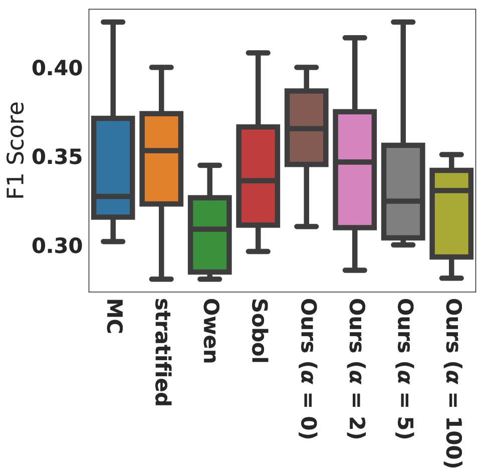
(a) Data Shapley (MNIST SVC)

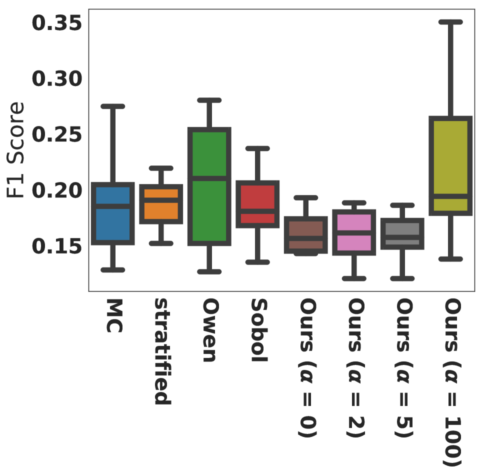
(b) Beta Shapley (breast cancer SVC)

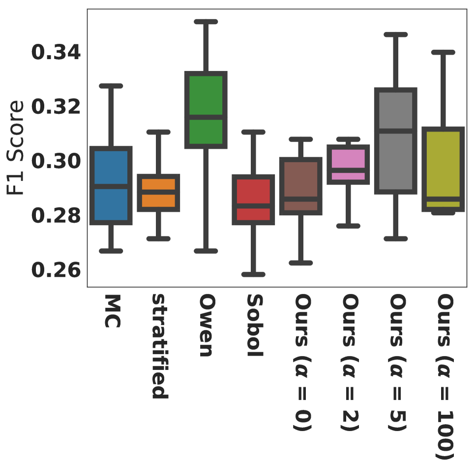
(c) Data Shapley (Gaussian SVC)

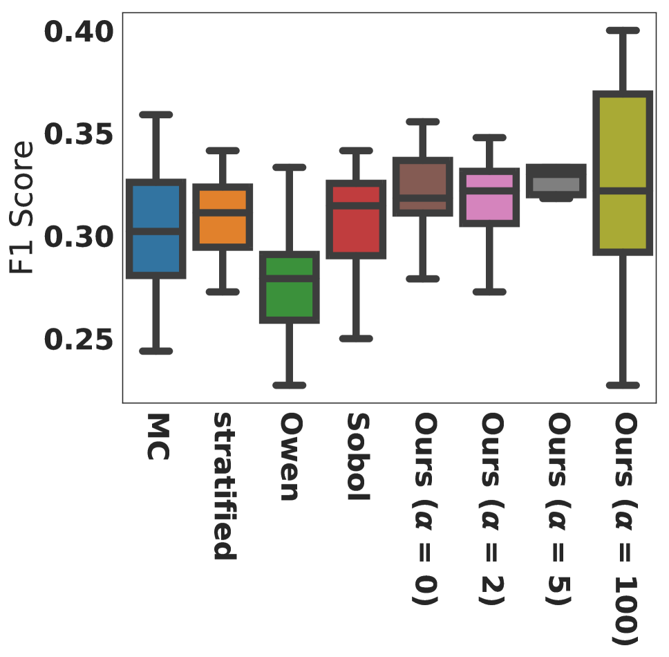
(d) Beta Shapley (Gaussian SVC)

Figure 5: Comparison between F1 score of noise detection task by various estimation methods on breast cancer and MNIST datasets. Caption of each plot shows the combination. KernelSHAP is omitted on MNIST dataset because its result is poor and obscures visualisation (medians are 0.194 on (a), 0.127 on (b), and 0.156 on (c) and (d)).

D.7 Training Example Addition and Removal

In addition to noisy label detection, Shapley value is also applied to find out the value of a training example in training a ML model, as demonstrated by the point addition and removal experiment. In addition, we perform more experiments on both Data Shapley and Beta Shapley. Results in Fig. 6 show most methods perform comparable except KernelSHAP. The performance of KernelSHAP can be attributed to its estimates are less accurate (as shown by its higher MAPEs and MSEs in previous tables), consistent with Fig. 3.

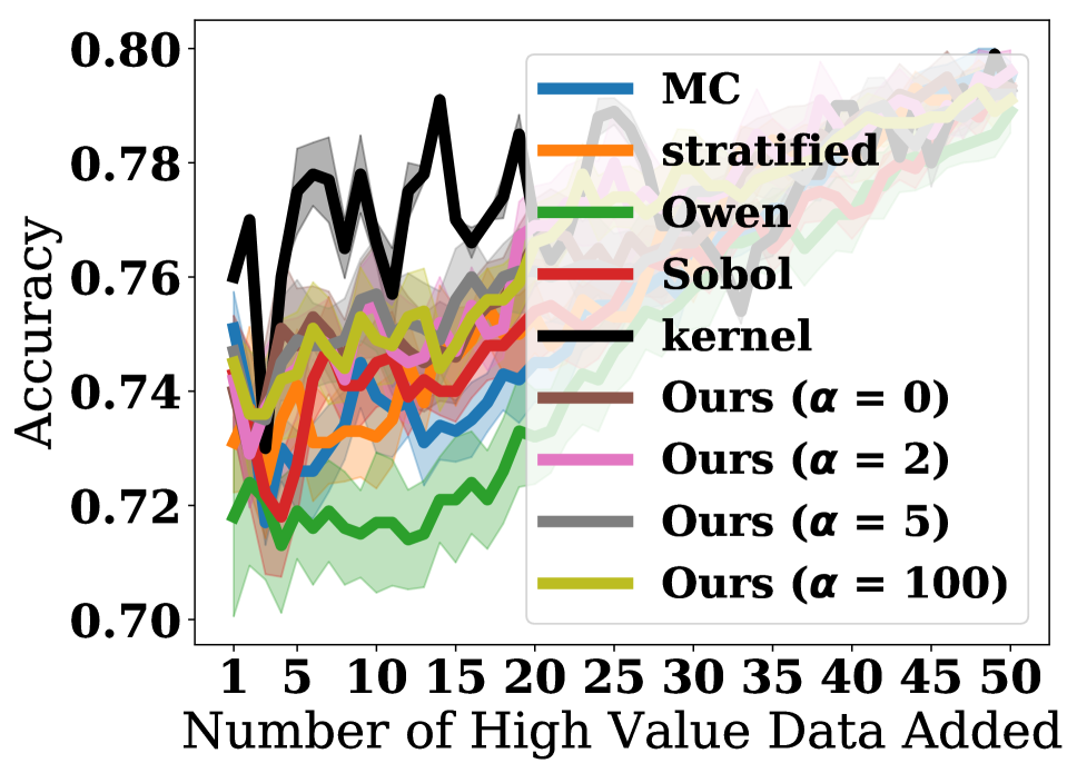
(a) Data Shapley (Add High Value Data)

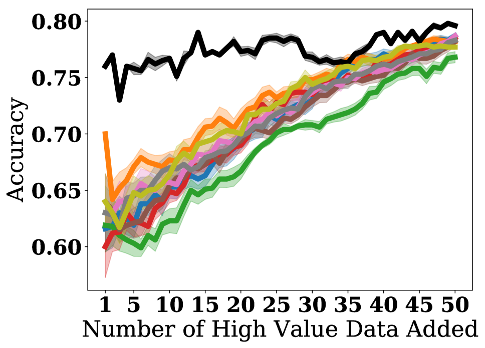
(b) Beta Shapley (Add High Value Data)

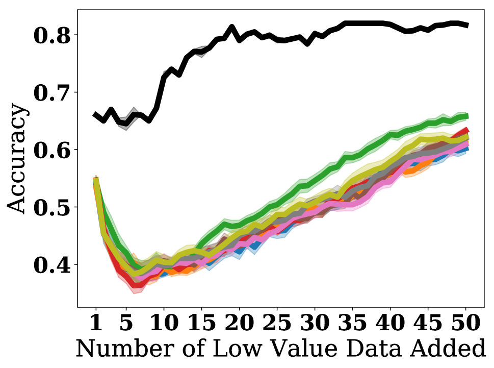
(c) Data Shapley (Add Low Value Data)

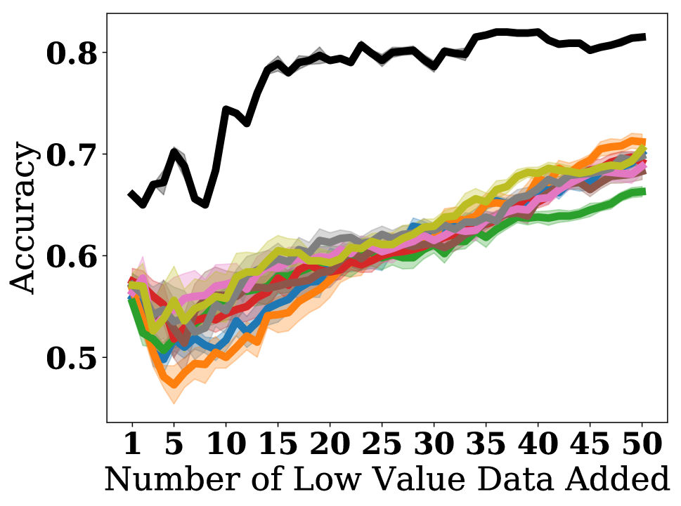
(d) Beta Shapley (Add Low Value Data)

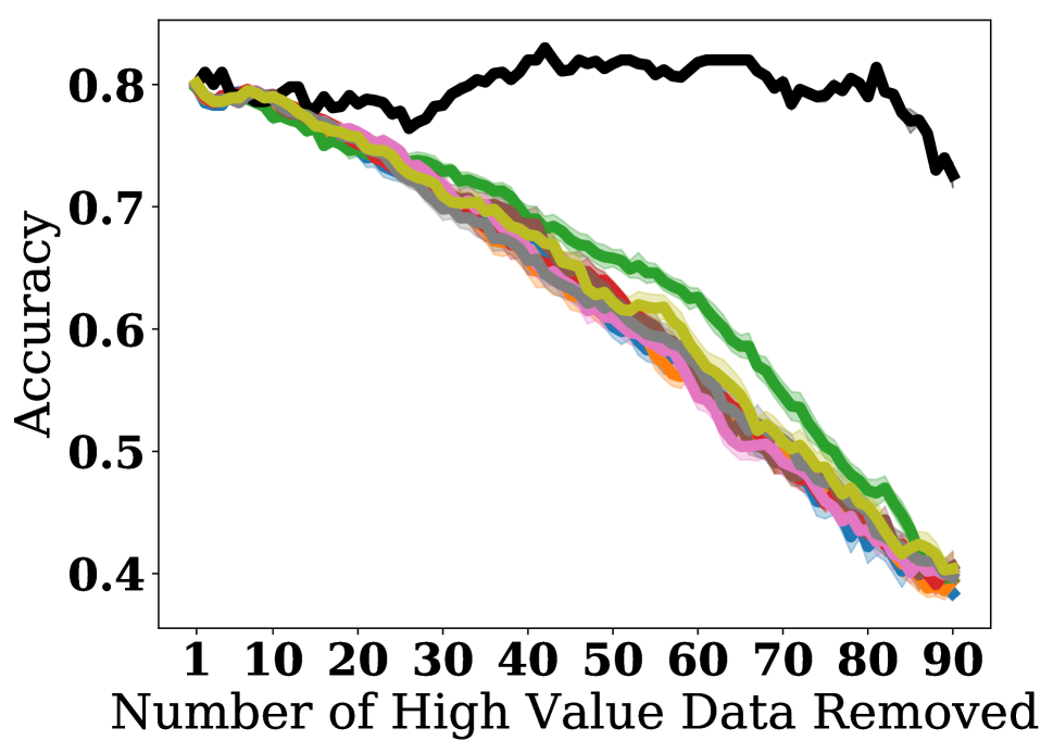
(e) Data Shapley (Remove High Value Data)

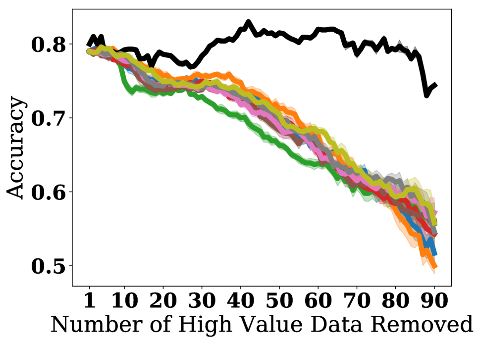
(f) Beta Shapley (Remove High Value Data)

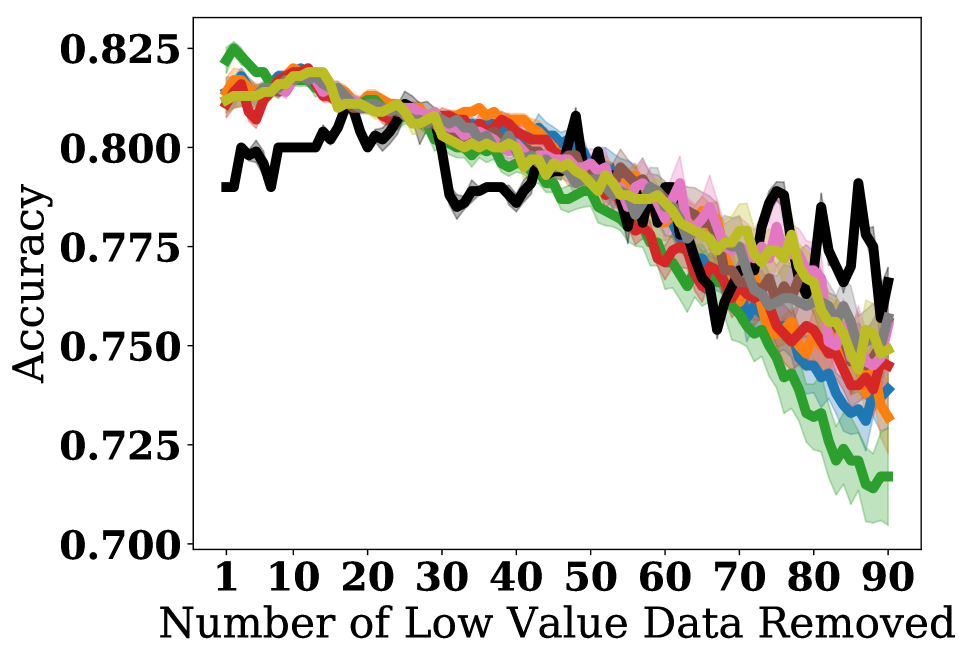
(g) Data Shapley (Remove Low Value Data)

(h) Beta Shapley (Remove Low Value Data)

Figure 6: Comparison between test accuracy by adding and removing data with large and small estimated Shapley value first (on synthetic Gaussian dataset trained on logistic regression classifier). Black lines represent KernelSHAP (omitted in main content). It can be observed that KernelSHAP does not produce a clear trend but stays horizontal in all plots.

References

- hot (2016) 2016. Trip Advisor hotel Reviews. URL https://www.kaggle.com/andrewmvd/trip-advisor-hotel-reviews.
- ube (2018) 2018. Uber and Lyft dataset Boston, MA. URL https://www.kaggle.com/brllrb/uber-and-lyft-dataset-boston-ma.
- use (2019) 2019. 100,000 UK used car dataset. URL https://www.kaggle.com/adityadesai13/used-car-dataset-ford-and-mercedes.
- cre (2019) 2019. Credit Card Fraud Detection. URL https://www.kaggle.com/mlg-ulb/creditcardfraud.
- Agarwal, Dahleh, and Sarkar (2019) Agarwal, A.; Dahleh, M.; and Sarkar, T. 2019. A marketplace for data: An algorithmic solution. In Proceedings of the ACM Conference on Economics and Computation, 701–726.
- Agussurja, Xu, and Low (2022) Agussurja, L.; Xu, X.; and Low, K. H. 2022. On the Convergence of the Shapley Value in Parametric Bayesian Learning Games. In Proceedings of the 39th International Conference on Machine Learning.
- Bahir et al. (1966) Bahir, M.; Peleg, B.; Maschler, M.; and Peleg, B. 1966. A characterization, existence proof and dimension bounds for the kernel of a game. Pacific Journal of Mathematics, 18.
- Bian et al. (2022) Bian, Y.; Rong, Y.; Xu, T.; Wu, J.; Krause, A.; and Huang, J. 2022. Energy-Based Learning for Cooperative Games, with Applications to Valuation Problems in Machine Learning. In International Conference on Learning Representations.
- Blackard (1998) Blackard, J. 1998. Covertype. UCI Machine Learning Repository.
- Castro, Gómez, and Tejada (2009) Castro, J.; Gómez, D.; and Tejada, J. 2009. Polynomial Calculation of the Shapley Value Based on Sampling. Computers & Operations Research, 36(5): 1726–1730.
- Castro et al. (2017) Castro, J.; Gómez, D.; Molina, E.; and Tejada, J. 2017. Improving polynomial estimation of the Shapley value by stratified random sampling with optimum allocation. Computers and Operations Research, 82: 180–188.
- Chalkiadakis, Elkind, and Wooldridge (2011) Chalkiadakis, G.; Elkind, E.; and Wooldridge, M. 2011. Computational Aspects of Cooperative Game Theory (Synthesis Lectures on Artificial Intelligence and Machine Learning). Morgan & Claypool Publishers, 1st edition.
- Covert and Lee (2021) Covert, I.; and Lee, S.-I. 2021. Improving KernelSHAP: Practical Shapley Value Estimation via Linear Regression. In Proceedings of the International Conference on Artificial Intelligence and Statistics.
- Dalton (1920) Dalton, H. 1920. The Measurement of the Inequality of Incomes. The Economic Journal, 30(119): 348–361.
- de Boer et al. (2003) de Boer, J. F.; Cense, B.; Park, B. H.; Pierce, M. C.; Tearney, G. J.; and Bouma, B. E. 2003. Improved signal-to-noise ratio in spectral-domain compared with time-domain optical coherence tomography. Optics Letters.
- de Clippel (2010) de Clippel, G. 2010. Comment on “The Veil of Public Ignorance”. Working paper.
- Deng (2012) Deng, L. 2012. The mnist database of handwritten digit images for machine learning research. IEEE Signal Processing Magazine, 29(6): 141–142.
- Efron et al. (2004) Efron, B.; Hastie, T.; Johnstone, I.; and Tibshirani, R. 2004. Least angle regression. The Annals of Statistics, 32(2).
- Efron and Tibshirani (1994) Efron, B.; and Tibshirani, R. J. 1994. An introduction to the bootstrap. CRC press.
- Elvira and Martino (2022) Elvira, V.; and Martino, L. 2022. Advances in Importance Sampling. arXiv:2102.05407.
- Fisher (1988) Fisher, R. A. 1988. Iris. UCI Machine Learning Repository.
- Forina et al. (1991) Forina, M.; et al. 1991. Wine. UCI Machine Learning Repository.
- Ghorbani, Kim, and Zou (2020) Ghorbani, A.; Kim, M. P.; and Zou, J. Y. 2020. A Distributional Framework for Data Valuation. In Proceedings of the International Conference on Machine Learning.
- Ghorbani and Zou (2019) Ghorbani, A.; and Zou, J. 2019. Data Shapley: Equitable Valuation of Data for Machine Learning. In Proceedings of the International Conference on Machine Learning, 2242–2251.
- Ghorbani, Zou, and Esteva (2021) Ghorbani, A.; Zou, J.; and Esteva, A. 2021. Data Shapley Valuation for Efficient Batch Active Learning. arXiv:2104.08312.
- Jia et al. (2019) Jia, R.; Dao, D.; Wang, B.; Hubis, F. A.; Gurel, N. M.; Li, B.; Zhang, C.; Spanos, C. J.; and Song, D. 2019. Efficient Task-Specific Data Valuation for Nearest Neighbor Algorithms. In Proceedings of the VLDB Endowment, 1610–1623.
- Jia et al. (2019) Jia, R.; Dao, D.; Wang, B.; Hubis, F. A.; Hynes, N.; Gürel, N. M.; Li, B.; Zhang, C.; Song, D.; and Spanos, C. J. 2019. Towards Efficient Data Valuation Based on the Shapley Value. In Proceedings of the International Conference on Artificial Intelligence and Statistics, 1167–1176.
- Kaneko and Nakamura (1979) Kaneko, M.; and Nakamura, K. 1979. The Nash Social Welfare Function. Econometrica, 47: 423–435.
- Kim (2014) Kim, Y. 2014. Convolutional Neural Networks for Sentence Classification. In Proceedings of the Conference on Empirical Methods in Natural Language Processing.
- Kloek, Kloek, and Van Dijk (1978) Kloek, T.; Kloek, T.; and Van Dijk, H. 1978. Bayesian Estimates of Equation System Parameters: An Application of Integration by Monte Carlo. Econometrica, 46: 1–19.
- Kohavi and Becker (1996) Kohavi, R.; and Becker, B. 1996. Adult. UCI Machine Learning Repository.
- Krizhevsky, Sutskever, and Hinton (2012) Krizhevsky, A.; Sutskever, I.; and Hinton, G. E. 2012. ImageNet Classification with Deep Convolutional Neural Networks. In Advances in Neural Information Processing Systems.
- Kwon and Zou (2022) Kwon, Y.; and Zou, J. 2022. Beta Shapley: a Unified and Noise-reduced Data Valuation Framework for Machine Learning. In Proceedings of the International Conference on Artificial Intelligence and Statistics.
- LeCun et al. (1990) LeCun, Y.; Boser, B.; Denker, J.; Henderson, D.; Howard, R.; Hubbard, W.; and Jackel, L. 1990. Handwritten Digit Recognition with a Back-Propagation Network. In Advances in Neural Information Processing Systems.
- Lundberg and Lee (2017) Lundberg, S. M.; and Lee, S.-I. 2017. A Unified Approach to Interpreting Model Predictions. In Advances in Neural Information Processing Systems, 4765–4774.
- Maleki et al. (2013) Maleki, S.; Tran-Thanh, L.; Hines, G.; Rahwan, T.; and Rogers, A. 2013. Bounding the Estimation Error of Sampling-based Shapley Value Approximation With/Without Stratifying.
- Mitchell et al. (2022) Mitchell, R.; Cooper, J.; Frank, E.; and Holmes, G. 2022. Sampling Permutations for Shapley Value Estimation. Journal of Machine Learning Research, 23(43): 1–46.
- Nguyen, Low, and Jaillet (2022) Nguyen, Q. P.; Low, K. H.; and Jaillet, P. 2022. Trade-off between Payoff and Model Rewards in Shapley-Fair Collaborative Machine Learning. In Advances in Neural Information Processing Systems.
- Ohrimenko, Tople, and Tschiatschek (2019) Ohrimenko, O.; Tople, S.; and Tschiatschek, S. 2019. Collaborative Machine Learning Markets with Data-Replication-Robust Payments. In Proceedings of the NeurIPS SGO & ML Workshop.
- Okhrati and Lipani (2020) Okhrati, R.; and Lipani, A. 2020. A Multilinear Sampling Algorithm to Estimate Shapley Values. In Proceedings of the International Conference on Pattern Recognition.
- Owen (1972) Owen, G. 1972. Multilinear Extensions of Games. Source: Management Science, 18: 64–79.
- Pang and Lee (2005) Pang, B.; and Lee, L. 2005. Seeing Stars: Exploiting Class Relationships for Sentiment Categorization with Respect to Rating Scales. In Proceedngs of the Annual Meeting of the Association for Computational Linguistics.
- Pennington, Socher, and Manning (2014) Pennington, J.; Socher, R.; and Manning, C. D. 2014. GloVe: Global Vectors for Word Representation. In Proceedings of the Empirical Methods in Natural Language Processing, 1532–1543.
- Rose (2012) Rose, A. 2012. Vision: Human and Electronic. Optical Physics and Engineering. Springer US. ISBN 9781468420395.
- Rozemberczki et al. (2022) Rozemberczki, B.; Watson, L.; Bayer, P.; Yang, H.-T.; Kiss, O.; Nilsson, S.; and Sarkar, R. 2022. The Shapley Value in Machine Learning. In Proceedings of the International Joint Conference on Artificial Intelligence. Survey Track.
- Sim, Xu, and Low (2022) Sim, R. H. L.; Xu, X.; and Low, K. H. 2022. Data Valuation in Machine Learning: ”Ingredients”, Strategies, and Open Challenges. In Proceedings of the International Joint Conference on Artificial Intelligence. Survey Track.
- Sim et al. (2020) Sim, R. H. L.; Zhang, Y.; Chan, M. C.; and Low, K. H. 2020. Collaborative Machine Learning with Incentive-Aware Model Rewards. In Proceedings of the International Conference on Machine Learning.
- Song, Tong, and Wei (2019) Song, T.; Tong, Y.; and Wei, S. 2019. Profit Allocation for Federated Learning. In Proceedings of the IEEE International Conference on Big Data, 2577–2586.
- Street (1995) Street, N. 1995. UCI Machine Learning Repository Breast Cancer Wisconsin (Diagnostic) Data Set.
- Sundararajan and Najmi (2020) Sundararajan, M.; and Najmi, A. 2020. The Many Shapley Values for Model Explanation. In Proceedings of the International Conference on Machine Learning, 9269–9278. PMLR.
- Sutton and Barto (2018) Sutton, R. S.; and Barto, A. G. 2018. Reinforcement Learning: An Introduction. The MIT Press.
- Tay et al. (2022) Tay, S.; Xu, X.; Foo, C. S.; and Low, K. H. 2022. Incentivizing Collaboration in Machine Learning via Synthetic Data Rewards. Proceedings of the AAAI Conference on Artificial Intelligence, 36(9): 9448–9456.
- Wang et al. (2020) Wang, T.; Rausch, J.; Zhang, C.; Jia, R.; and Song, D. 2020. A Principled Approach to Data Valuation for Federated Learning. Lecture Notes in Computer Science, 12500: 153–167.
- Wang, Yang, and Jia (2021) Wang, T.; Yang, Y.; and Jia, R. 2021. Learnability of Learning Performance and Its Application to Data Valuation. arXiv:2107.06336.
- Wu, Shu, and Low (2022) Wu, Z.; Shu, Y.; and Low, K. H. 2022. DAVINZ: Data Valuation using Deep Neural Networks at Initialization. In Proceedings of the International Conference on Machine Learning.
- Xu et al. (2021a) Xu, X.; Lyu, L.; Ma, X.; Miao, C.; Foo, C. S.; and Low, K. H. 2021a. Gradient driven rewards to guarantee fairness in collaborative machine learning. In Advances in Neural Information Processing Systems.
- Xu et al. (2021b) Xu, X.; Wu, Z.; Foo, C. S.; and Low, K. H. 2021b. Validation free and replication robust volume-based data valuation. In Advances in Neural Information Processing Systems.
- Yuan and Druzdzel (2007) Yuan, C.; and Druzdzel, M. J. 2007. Theoretical Analysis and Practical Insights on Importance Sampling in Bayesian Networks. International Journal of Approximate Reasoning, 46(2): 320–333.