Scalable and adaptive variational Bayes methods for Hawkes processes

Abstract

Hawkes processes are often applied to model dependence and interaction phenomena in multivariate event data sets, such as neuronal spike trains, social interactions, and financial transactions. In the nonparametric setting, learning the temporal dependence structure of Hawkes processes is generally a computationally expensive task, all the more with Bayesian estimation methods. In particular, for generalised nonlinear Hawkes processes, Monte-Carlo Markov Chain methods applied to compute the doubly intractable posterior distribution are not scalable to high-dimensional processes in practice. Recently, efficient algorithms targeting a mean-field variational approximation of the posterior distribution have been proposed. In this work, we first unify existing variational Bayes approaches under a general nonparametric inference framework, and analyse the asymptotic properties of these methods under easily verifiable conditions on the prior, the variational class, and the nonlinear model. Secondly, we propose a novel sparsity-inducing procedure, and derive an adaptive mean-field variational algorithm for the popular sigmoid Hawkes processes. Our algorithm is parallelisable and therefore computationally efficient in high-dimensional setting. Through an extensive set of numerical simulations, we also demonstrate that our procedure is able to adapt to the dimensionality of the parameter of the Hawkes process, and is partially robust to some type of model mis-specification.

Keywords: temporal point processes, bayesian nonparametrics, connectivity graph, variational approximation.

1 Introduction

Modelling point or event data with temporal dependence often implies to infer a local dependence structure between events and to estimate interaction parameters. In this context, the multivariate Hawkes process is a widely used temporal point process (TPP) model, for instance, in seismology (Ogata, 1999), criminology (Mohler et al., 2011), finance (Bacry and Muzy, 2015), and social network analysis (Lemonnier and Vayatis, 2014). In particular, the generalised nonlinear multivariate Hawkes model, an extension of the classical self-exciting process (Hawkes, 1971), is able to account for different types of temporal interactions, including excitation and inhibition effects, often found in event data (Hawkes, 2018; Bonnet et al., 2021). The excitation phenomenon, sometimes named contagion or bursting behaviour, corresponds to empirical observation that the occurrence of an event, e.g., a post on a social media, increases the probability of observing similar events in the future, e.g., reaction comments. The inhibition phenomenon refers to the opposite observation and is prominent in neuronal applications due to biological regulation mechanisms (Bonnet et al., 2021), and in criminology due to the enforcement of policies (Olinde and Short, 2020). Moreover, the Hawkes model has become popular for the interpretability of its parameter, in particular the connectivity or dependence graph parameter, which corresponds to a Granger-causal graph for the multivariate point process (Eichler et al., 2017).

More precisely, in event data modelling, a multivariate TPP is often described as a counting process of events (or points), $N=(N_{t})_{t\in[0,T]}=(N_{t}^{1},\dots,N_{t}^{K})_{t\in[0,T]}$, where $K\geqslant 1$ is the number of components (or dimensions) of the process, observed over a period $[0,T]$ of length $T>0$. Each component of a TPP can represent a specific type of event (e.g., an earthquake), or a particular location where events are recorded (e.g., a country). For each $k=1,\dots,K$ and time $t\in[0,T]$, $N_{t}^{k}\in\varmathbb{N}$ counts the number of events that have occurred until $t$ at component $k$, therefore, $(N_{t}^{k})_{t\in[0,T]}$ is an integer-valued, non-decreasing, process. In particular, multivariate TPP models are of interest for jointly modelling the occurrences of events separated into distinct types, or recorded at multiple places, by specifying a multivariate conditional intensity function (or, more concisely, intensity). The latter, denoted $(\lambda_{t})_{t}=(\lambda_{t}^{1},\dots,\lambda_{t}^{K})_{t\in\varmathbb R}$, characterises the probability distribution of events, for each component. It is informally defined as the infinitesimal probability rate of event, conditionally on the history of the process, i.e,

$$\lambda_{t}^{k}dt=\operatorname*{\varmathbb{P}}\left[\text{event at dimension $k$ in }\>[t,t+dt]\Big{|}\mathcal{G}_{t}\right],\quad k=1,\dots,K,\quad t\in[0,T],$$

where $\mathcal{G}_{t}=\sigma(N_{s},0\leqslant s<t)$ denotes the history of the process until time $t$. In the generalised nonlinear Hawkes model, the intensity is defined as

$$\lambda_{t}^{k}=\phi_{k}\left(\nu_{k}+\sum_{l=1}^{K}\int_{-\infty}^{t^{-}}h_{lk}(t-s)dN_{s}^{l}\right),\quad k=1,\dots K,$$ (1)

where for each $k$, $\phi_{k}:\varmathbb{R}\to\varmathbb{R}^{+}$ is a link or activation function, $\nu_{k}>0$ is a background or spontaneous rate of events, and for each $l=1,\dots,K$, $h_{lk}:\varmathbb R^{+}\to\varmathbb R$ is an interaction function or triggering kernel, modelling the influence of $N^{l}$ onto $N^{k}$. We note that in this model, the parameter $\nu=(\nu_{k})_{k}$ characterises the external influence of the environment on the process, here, assumed constant over time, while the functions $h=(h_{lk})_{l,k=1,\dots,K}$ parametrise the causal influence of past events, that depends on each ordered pair of dimensions. In particular, for any $(l,k)$, there exists a Granger-causal relationship from $N^{l}$ to $N^{k}$, or in other words, $N^{k}$ is locally-dependent on $N^{l}$, if and only if $h_{lk}\neq 0$ (Eichler et al., 2017). Moreover, defining for each $(l,k)$, $\delta_{lk}:=\mathds{1}_{h_{lk}\neq 0}$, the parameter $\delta:=(\delta_{lk})_{l,k}\in\{0,1\}^{K\times K}$ defines a Granger-causal graph, called the connectivity graph.

Finally, the link functions $\phi=(\phi_{k})_{k}$’s are in general nonlinear and monotone non-decreasing, so that a value $h_{lk}(x)>0$ can be interpreted as an excitation effect, and $h_{lk}(x)<0$ as an inhibition effect, for some $x\in\varmathbb R^{+}$. Link functions are an essential part of the model chosen by the practitioner, and frequently set as ReLU functions $\phi_{k}(x)=\max(x,0)=(x)_{+}$ (Hansen et al., 2015; Chen et al., 2017a; Costa et al., 2020; Lu and Abergel, 2018; Bonnet et al., 2021; Deutsch and Ross, 2022), sigmoid-type functions, e.g., $\phi_{k}(x)=\theta_{k}(1+e^{x})^{-1}$ with a scale parameter $\theta_{k}>0$ (Zhou et al., 2021b, a; Malem-Shinitski et al., 2021), softplus functions $\phi_{k}(x)=\log(1+e^{x})$ (Mei and Eisner, 2017), or clipped exponential functions, i.e., $\phi_{k}(x)=\min(e^{x},\Lambda_{k})$ with a clip parameter $\Lambda_{k}>0$ (Gerhard et al., 2017; Carstensen et al., 2010). When all the interaction functions are non-negative and $\phi_{k}(x)=x$ for every $k$, the intensity (1) corresponds to the linear Hawkes model. Defining the underlying or linear intensity as

$$\tilde{\lambda}_{t}^{k}=\nu_{k}+\sum_{l=1}^{K}\int_{-\infty}^{t^{-}}h_{lk}(t-s)dN_{s}^{l},\quad k=1,\dots,K,$$ (2)

for any $t\in\varmathbb R$, the nonlinear intensity (1) can be re-written as $\lambda_{t}^{k}=\phi_{k}(\tilde{\lambda}_{t}^{k})$.

Estimating the parameter of the Hawkes model, denoted $f=(\nu,h)$, and the graph parameter $\delta$, can be done via Bayesian nonparametric methods, by leveraging standard prior distributions such as random histograms, B-splines, mixtures of Beta densities (Donnet et al., 2020; Sulem et al., 2021), or Gaussian processes (Malem-Shinitski et al., 2021), which enjoy asymptotic guarantees under mild conditions on the model. However, Monte-Carlo Markov Chain (MCMC) methods to compute the posterior distribution are too computationally expensive in practice, even in linear Hawkes models with a moderately large number of dimensions (Donnet et al., 2020). In contrast, frequentist methods such as maximum likelihood estimates (Bonnet et al., 2021) and penalised projection estimators (Hansen et al., 2015; Bacry et al., 2020; Cai et al., 2021) are more computationally efficient but do not provide uncertainty quantification on the parameter estimates. Yet, in practice, most methods rely on estimating a parametric exponential form of the interaction functions, i.e., $h_{lk}(x)=\alpha_{lk}e^{-\beta_{lk}x}$ (Bonnet et al., 2021; Wang et al., 2016; Deutsch and Ross, 2022).

The implementation of Bayesian methods using MCMC algorithms is computational intensive for two reasons: the high dimensionality of the parameter space ($K^{2}$ functions and $K$ parameters to estimate) and the non linearity induced by the link function. Recently, data augmentation strategies have been used to answer the second difficulty, jointly with variational Bayes algorithms in sigmoid Hawkes processes (Malem-Shinitski et al., 2021; Zhou et al., 2022). These novel methods leverage the conjugacy of an augmented mean-field variational posterior distribution with certain families of Gaussian priors. In particular, Zhou et al. (2021a) propose an efficient iterative mean-field variational inference (MF-VI) algorithm in a semi-parametric multivariate model. A similar type of algorithm is introduced by Malem-Shinitski et al. (2021), based on a nonparametric Gaussian process prior construction. Nonetheless, these methods do not consider the high-dimensional nonparametric setting. They do not address either the problem of estimating the connectivity graph $\delta$, which is of interest in many applications and which also allows to reduce the computational complexity. In fact, the connectivity graph also determines the dimensionality and the sparsity of the estimation problem, similarly to the structure parameter in high-dimensional regression (Ray and Szabó, 2021). Moreover, variational Bayes approaches have not been yet theoretically analysed.

In this work, we make the following contributions to the variational Bayes estimation of multivariate Hawkes processes.

• First, we provide a general nonparametric variational Bayes estimation framework for multivariate Hawkes processes and analyse the asymptotic properties of variational methods in this context. We notably establish concentration rates for variational posterior distributions, leveraging the general methodology of Zhang and Gao (2020), based on verifying a prior mass, a testing, and a variational class condition. Moreover, we apply our general results to variational classes of interest in the Hawkes model, namely mean-field and model-selection variational families.

• Secondly, we propose a novel adaptive and sparsity-inducing variational Bayes procedure, based on a estimate of the connectivity graph using thresholding of the $\ell_{1}$-norms of the interaction functions, and relying on model selection variational families (Zhang and Gao, 2020; Ohn and Lin, 2021). For sigmoid Hawkes processes, we additionally leverage a mean-field approximation to derive an efficient adaptive variational inference algorithm. In addition to being theoretically valid in the asymptotic regime, we show that this approach performs very well in practice.

• In addition to the previous theoretical guarantees and proposed methodology, we empirically demonstrate the effectiveness of our algorithm in an extensive set of simulations. We notably show that, in low-dimensional settings, our adaptive variational algorithm is more computationally efficient than MCMC methods, while enjoying comparable estimation performance. Moreover, our approach is scalable to high-dimensional and sparse processes, and provides good estimates. In particular, our algorithm is able to uncover the causality structure of the true generating process given by the graph parameter, even in some type of model mis-specification.

Outline

In the remaining part of this section, we introduce some useful notation. Then, in Section 2, we describe our general model and inference setup, and present our novel adaptive and sparsity-inducing variational algorithm in Section 3. Moreover, Section 4 contains our general results, and their applications to prior and variational families of interest in the Hawkes model. Finally, we report in Section 5 the results of an in-depth simulation study. Besides, the proofs of our main results are reported in Appendix D.

Notations. For a function $h$, we denote $\left\lVert h\right\rVert_{1}=\int_{\varmathbb R}|h(x)|dx$ the $L_{1}$-norm, $\left\lVert h\right\rVert_{2}=\sqrt{\int_{\varmathbb R}h^{2}(x)dx}$ the $L_{2}$-norm, $\left\lVert h\right\rVert_{\infty}=\sup\limits_{x\in\varmathbb R}|h(x)|$ the supremum norm, and $h^{+}=max(h,0),\>h^{-}=max(-h,0)$ its positive and negative parts. For a $K\times K$ matrix $M$, we denote $r(M)$ its spectral radius, $\left\lVert M\right\rVert$ its spectral norm, and $tr(M)$ its trace. For a vector $u\in\varmathbb R^{K},\left\lVert u\right\rVert_{1}=\sum_{k=1}^{K}|u_{k}|$. The notation $k\in[K]$ is used for $k\in\{1,\ldots,K\}$. For a set $B$ and $k\in[K]$, we denote $N^{k}(B)$ the number of events of $N^{k}$ in $B$ and $N^{k}|_{B}$ the point process measure restricted to the set $B$. For random processes, the notation $\overset{\mathcal{L}}{=}$ corresponds to equality in distribution. We also denote $\mathcal{N}(u,\mathcal{H}_{0},d)$ the covering number of a set $\mathcal{H}_{0}$ by balls of radius $u$ w.r.t. a metric $d$. For any $k\in[K]$, let $\mu_{k}^{0}=\varmathbb{E}_{0}[\lambda_{t}^{k}(f_{0})]$ be the mean of $\lambda_{t}^{k}(f_{0})$ under the stationary distribution $\varmathbb{P}_{0}$. For a set $\Omega$, its complement is denoted $\Omega^{c}$. We also use the notations $u_{T}\lesssim v_{T}$ if $|u_{T}/v_{T}|$ is bounded when $T\to\infty$, $u_{T}\gtrsim v_{T}$ if $|v_{T}/u_{T}|$ is bounded and $u_{T}\asymp v_{T}$ if $|u_{T}/v_{T}|$ and $|v_{T}/u_{T}|$ are bounded. We recall that a function $\phi$ is $L$-Lipschitz, if for any $(x,x^{\prime})\in\varmathbb R^{2}$, $|\phi(x)-\phi(x^{\prime})|\leqslant L|x-x^{\prime}|$. We denote $\mathds{1}_{n}$ and $\mathbf{0}_{n}$ the all-ones and all-zeros vectors of size $n$. Finally, we denote $\mathcal{H}(\beta,L_{0})$ the Hölder class of $\beta$-smooth functions with radius $L_{0}$.

2 Bayesian nonparametric inference of multivariate Hawkes processes

2.1 The Hawkes model and Bayesian framework

Formally a $K$-dimensional temporal point process $N=(N_{t})_{t\in\varmathbb R}=(N_{t}^{1},\dots,N_{t}^{K})_{t\in\varmathbb R}$, defined as a process on the real line $\varmathbb R$ and on a probability space $(\mathcal{X},\mathcal{G},\varmathbb{P})$, is a Hawkes process if it satisfies the following properties.

1. Almost surely, $\forall k,l\in[K]$, $(N^{k}_{t})_{t}$ and $(N^{l}_{t})_{t}$ never jump simultaneously.

2. For all $k\in[K]$, the $\mathcal{G}_{t}$-predictable conditional intensity function of $N^{k}$ at $t\in\varmathbb R$ is given by (1), where $\mathcal{G}_{t}=\sigma(N_{s},s<t)\subset\mathcal{G}$.

From now on, we assume that $N$ is a stationary, finite-memory, $K$-dimensional Hawkes process $N$ with parameter $f_{0}=(\nu_{0},h_{0})$, link functions $(\phi_{k})_{k}$, and memory parameter $A>0$, defined as $A=\sup\{x\in\varmathbb R^{+};\max_{l,k}|h_{lk}^{0}(x)|>0\}$. We note that $A$ characterises the temporal length of interaction of the point process and that this inference setting is commonly used in previous work on Hawkes processes (Hansen et al., 2015; Donnet et al., 2020; Sulem et al., 2021; Cai et al., 2021). We assume that $f_{0}$ is the unknown parameter, and that $(\phi_{k})_{k}$ and $A$ are known to the statistician.

Similarly to Donnet et al. (2020), we consider that our data is an observation of $N$ over a time window $[-A,T]$, with $T>0$, but our inference procedure is based on the log-likelihood function corresponding to the observation of $N$ over $[0,T]$. For a parameter $f=(\nu,h)$, this log-likelihood is given by

$$L_{T}(f):=\sum_{k=1}^{K}L_{T}^{k}(f),\quad L_{T}^{k}(f)=\left[\int_{0}^{T}\log(\lambda_{t}^{k}(f))dN_{t}^{k}-\int_{0}^{T}\lambda_{t}^{k}(f)dt\right].$$ (3)

We denote by $\varmathbb{P}_{0}(.|\mathcal{G}_{0})$ the true conditional distribution of $N$, given the initial condition $\mathcal{G}_{0}$, and by $\varmathbb{P}_{f}(.|\mathcal{G}_{0})$ the distribution defined as $d\varmathbb{P}_{f}(.|\mathcal{G}_{0})=e^{L_{T}(f)-L_{T}(f_{0})}\varmathbb{P}_{0}(.|\mathcal{G}_{0}).$ We also denote $\varmathbb{E}_{0}$ and $\varmathbb{E}_{f}$ the expectations associated to $\varmathbb{P}_{0}(.|\mathcal{G}_{0})$ and $\varmathbb{P}_{f}(.|\mathcal{G}_{0})$. With a slight abuse of notation, we drop the notation $\mathcal{G}_{0}$ in the subsequent expressions.

We consider a nonparametric setting for estimating the parameter $f$, within a parameter space $\mathcal{F}$. Given a prior distribution $\Pi$ on $\mathcal{F}$, the posterior distribution, for any subset $B\subset\mathcal{F}$, is defined as

$$\Pi(B|N)=\frac{\int_{B}\exp(L_{T}(f))d\Pi(f)}{\int_{\mathcal{F}}\exp(L_{T}(f))d\Pi(f)}=:\frac{N_{T}(B)}{D_{T}},\quad D_{T}:=\int_{\mathcal{F}}\exp(L_{T}(f))d\Pi(f).$$ (4)

This posterior distribution (4) is often said to be doubly intractable, because of the integrals in the log-likelihood function (3) and in the denominator $D_{T}$. Before studying the problem of computing the posterior distribution, we explicit our construction of the prior distribution.

Firstly, our prior distribution $\Pi$ is built so that it puts mass 1 to finite-memory processes, i.e., to parameter $f$ such that the interaction functions $(h_{lk})_{l,k}$ have a bounded support included in $[0,A]$. Moreover, we use a hierarchical spike-and-slab prior based on the connectivity graph parameter $\delta$ similar to Donnet et al. (2020); Sulem et al. (2021). For each $(l,k)\in[K]^{2}$, we consider the following parametrisation

$$h_{lk}=\delta_{lk}\bar{h}_{lk},\quad\delta_{lk}\in\{0,1\},\quad\text{ with }\quad\bar{h}_{lk}=0\quad\iff\quad\delta_{lk}=0$$

so that $\delta=(\delta_{lk})_{lk}\in\{0,1\}^{K^{2}}$ is the connectivity graph associated to $f$. We therefore consider $\delta\sim\Pi_{\delta}$, where $\Pi_{\delta}$ is a prior distribution on the space $\{0,1\}^{K^{2}}$, and, for each $(l,k)$ such that $\delta_{lk}=1$, $\bar{h}_{lk}\sim\tilde{\Pi}_{h}$ where $\tilde{\Pi}_{h}$ is a prior distribution on functions with support included in $[0,A]$. In this paper we will mostly consider the case where the functions $\bar{h}_{lk}$, when non null, are developed on a dictionary of functions $(e_{j})_{j\geqslant 1}$, such that $e_{j}:[0,A]\to\varmathbb R,\>\forall j$, and

$$\bar{h}_{lk}=\sum_{j=1}^{J_{k}}h_{lk}^{j}e_{j},\quad h_{lk}^{j}\in\varmathbb R,\>\quad\forall j\in[J_{k}],\quad J_{k}\geqslant 1,\quad(l,k)\in[K]^{2}.$$ (5)

Then, choosing a prior distribution $\Pi_{J}$ on $J=(J_{k})_{k\in[K]}$, our hierarchical prior on $f$ finally writes as

$$d\Pi(f)=d\Pi_{\nu}(\nu)d\Pi_{\delta}(\delta)d\Pi_{J}(J)d\Pi_{h|\delta,J}(h),$$ (6)

where $\Pi_{\nu}$ is a prior distribution on $\varmathbb R_{+}^{K}$, suitable to the nonlinear model (see Sulem et al. (2021) for some examples), and

$$d\Pi_{h|\delta,J}(h)=\prod_{l,k}(1-\delta_{lk})\delta_{(0)}(\bar{h})+\delta_{lk}d\tilde{\Pi}_{h|\delta,J}(\bar{h}),$$

where $\delta_{(0)}$ denotes the Dirac measure at 0 and $\tilde{\Pi}_{h|\delta,J}(\bar{h})$ is a prior distribution on non-null functions decomposed over $J_{k}$ functions from the dictionary. From the previous construction, one can see that the graph parameter $\delta\in\{0,1\}^{K^{2}}$ defines the sparsity structure of $h=(h_{lk})_{l,k}$. This parameter plays a crucial role when performing inference on high dimensional Hawkes processes, either in settings when sparsity is a reasonable assumption, or as the only parameter of interest (Bacry et al., 2020; Chen et al., 2017b).

As previously noted, it is generally expensive to compute the posterior distribution (4), which does not have an analytical expressions. However, we note that when the prior on $f$ is a product of probability distributions on the dimension-restricted parameters $f_{k}=(\nu_{k},(h_{lk})_{l=1,\dots,K})\in\mathcal{F}_{k}$, for $k\in[K]$, so that $f=(f_{k})_{k}$, $\mathcal{F}=\mathcal{F}_{1}\times\dots\times\mathcal{F}_{K}$ and $d\Pi(f)=\prod_{k}d\Pi_{k}(f_{k})$, then, given the expressions of the log-likelihood function (3) and the intensity function (1), we have that each term $L_{T}^{k}(f)$ in (3) only depends on $f_{k}$, i.e., $L_{T}^{k}(f)=L_{T}^{k}(f_{k})$. Furthermore, the posterior distribution can be written as

$$d\Pi(f|N)=\prod_{k}d\Pi_{k}(f_{k}|N),\quad d\Pi_{k}(f_{k}|N)=\frac{\exp(L_{T}^{k}(f_{k}))d\Pi_{k}(f_{k})}{\int_{\mathcal{F}_{k}}\exp(L_{T}^{k}(f_{k}))d\Pi_{k}(f_{k})}.$$ (7)

In particular, the latter factorisation implies that each factor $\Pi_{k}(.|N)$ of the posterior distribution can be computed in parallel, nonetheless, given the whole data $N$. Despite this possible parallelisation, implementation of MCMC methods for computing the posterior distribution in the context of multivariate nonlinear Hawkes processes remains very challenging (Donnet et al., 2020; Zhou et al., 2021a; Malem-Shinitski et al., 2021). To alleviate this computational bottleneck, we consider in the next section a family of variational algorithms, together with a two-step procedure to handle high-dimensional processes.

2.2 Variational Bayes inference

To scale up Bayesian nonparametric methods to high-dimensional processes, we consider a variational Bayes approach. The latter consists of approximating the posterior distribution within a variational class of distributions on $\mathcal{F}$, denoted $\mathcal{V}$. Then, the variational Bayes (VB) posterior distribution, denoted $\hat{Q}$, is defined as the best approximation of the posterior distribution within $\mathcal{V}$, with respect to the Kullback-Leibler divergence, i.e.,

$$\hat{Q}:=\arg\min_{Q\in\mathcal{V}}KL\left(Q||\Pi(.|N)\right),$$ (8)

where the Kullabck-Leibler divergence between $Q$ and $Q^{\prime}$ is defined as

$$KL(Q||Q^{\prime}):=\begin{cases}\int\log\Big{(}\frac{dQ}{dQ^{\prime}}\Big{)}dQ,&\text{if }Q\ll Q^{\prime}\\ +\infty,&\text{otherwise}\end{cases}.$$

For a more in-depth introduction to this framework in the context of Hawkes processes, we refer to the works of Zhang et al. (2020); Zhou et al. (2022); Malem-Shinitski et al. (2021).

In the variational Bayes approach, there are many possible families for $\mathcal{V}$. Interestingly, we note that under a product posterior (7), the variational distribution also factorises in $K$ factors, $\hat{Q}=\prod_{k}\hat{Q}_{k}$ where each factor $\hat{Q}_{k}$ approximates $\Pi_{k}(.|N)$. Therefore, one can choose a variational class $\mathcal{V}^{\prime}$ of distributions on $\mathcal{F}_{1}$, and define $\mathcal{V}:=\mathcal{V}^{\prime\otimes K}$. In the case of multivariate Hawkes processes, we combine mean-field variational approaches (Zhou et al., 2022; Malem-Shinitski et al., 2021) with different versions of model selection variational methods (Zhang and Gao, 2020; Ohn and Lin, 2021). Some important notions related to the two latter inference strategies are recalled in Appendix A. Before presenting our method, we introduce additional concepts and notation.

We consider a general model where the log-likelihood function of the nonlinear Hawkes process can be augmented with some latent variable $z\in\mathcal{Z}$, with $\mathcal{Z}$ the latent parameter space. This approach is notably used by Malem-Shinitski et al. (2021); Zhou et al. (2021a) in the sigmoid Hawkes model, for which $\phi_{k}(x)\propto(1+e^{x})^{-1},\forall k\in[K]$. Denoting $L_{T}^{A}(f,z)$ the augmented log-likelihood, we define the augmented posterior distribution as

$$\Pi_{A}(B|N)=\frac{\int_{B}\exp(L_{T}^{A}(f,z))d(\Pi(f)\times\varmathbb{P}_{A}(z))}{\int_{\mathcal{F}\times\mathcal{Z}}\exp(L_{T}^{A}(f,z))d(\Pi(f)\times\varmathbb{P}_{A})(z)},\quad B\subset\mathcal{F}\times\mathcal{Z},$$

where $\varmathbb{P}_{A}$ is a prior density on $\mathcal{Z}$ with respect to a dominating measure $\mu_{z}$. One can then define an approximating mean-field family of $\Pi_{A}(.|N)$ as

$$\mathcal{V}_{AMF}=\left\{Q:\mathcal{F}\times\mathcal{Z}\to[0,1];\>Q(f,z)=Q_{1}(f)Q_{2}(z)\right\},$$ (9)

by only “breaking” correlations between parameters and latent variables. The corresponding mean-field variational posterior distribution is then

$$\hat{Q}_{AMF}=\arg\min_{Q\in\mathcal{V}_{AMF}}KL(Q||\Pi_{A}(.|N)).$$ (10)

Moreover, our hierarchical prior construction (6) implies that a parameter $f$ is indexed by a set of hyperparameters in the form $m=(\delta,J_{lk};(l,k)\in\mathcal{I}(\delta))$, where $\mathcal{I}(\delta):=\{(l,k)\in[K]^{2};\,\delta_{lk}=1\}$ is the set of “edges”, i.e., pair indices corresponding to non-null interaction functions in $f$. Moreover, $J_{lk}$ is the number of functions in the dictionary used to decompose $h_{lk}$. We note that $m$ characterises the dimensionality of the parameter $f$, and we call it a model. We can then re-write our parameter space as

$$\mathcal{F}=\bigcup_{m\in\mathcal{M}}\mathcal{F}_{m},\quad\mathcal{F}_{m}=\left\{f^{\prime}\in\mathcal{F};\>\delta^{\prime}=\delta,\>J^{\prime}=J\right\},\quad m=(\delta,J),\>\delta=(\delta_{lk})_{l,k},\>J=(J_{lk})_{l,k},$$ (11)

where $\mathcal{M}$ is the set of models

$$\mathcal{M}=\left\{m=(\delta,J);\delta\in\{0,1\}^{K\times K},\>J\in\varmathbb N^{K\times K}\right\}.$$

From now on, we assume that for each $k$, $J_{lk}=J_{k},\>foralll$ and re-define $J=(J_{1},\dots,J_{K})\in\varmathbb N^{K}$.

The decomposition (11) of the parameter space is key to compute a variational distribution that has support on the whole space $\mathcal{F}$, and that in particular, provides a distribution on the space of graph parameter. Next, we can construct an adaptive variational posterior distribution by considering an approximating family of variational distributions within each subspace $\mathcal{F}_{m}$, denoted $\mathcal{V}^{m}$. We leverage two types of adaptive variational posterior distributions, $\hat{Q}_{A1}$ and $\hat{Q}_{A2}$, considered respectively by Zhang and Gao (2020) and Ohn and Lin (2021), and defined as

$$\hat{Q}_{A1}:=\hat{Q}_{\hat{m}},\quad\hat{m}:=\arg\max_{m\in\mathcal{M}}ELBO(\hat{Q}^{m}),$$ (12)

$$\hat{Q}_{A2}:=\sum_{m\in\mathcal{M}}\hat{\gamma}_{m}\hat{Q}_{m},$$ (13)

where $\hat{Q}_{m}=\arg\min_{Q\in\mathcal{V}^{m}}KL(Q|||\Pi(.|N))$ is the variational posterior distribution in model $m$ (defined on $\mathcal{F}_{m}$), $ELBO(\cdot)$ is the evidence lower bound (ELBO) (defined in our context in (34) in Appendix C.2), and $\{\hat{\gamma}_{m}\}_{m\in\mathcal{M}}$ are the model marginal probabilities defined as

$$\hat{\gamma}_{m}=\frac{\Pi_{m}(m)\exp\left\{ELBO(\hat{Q}_{m})\right\}}{\sum_{m\in\mathcal{M}}\Pi_{m}(m)\exp\left\{ELBO(\hat{Q}_{m})\right\}},\quad m\in\mathcal{M}.$$

Remark 1

We note that in practice one might prefer using the adaptive VB posterior (12) rather than (13), to avoid manipulating a distribution mixture. In our simulations in Section 5, we often find that one or two models only have significant marginal probabilities $\hat{\gamma}_{k}^{m}$, and therefore the two adaptive variational posteriors (12) and (13) are often close.

To leverage the computational benefits of the augmented mean-field variational class (9), we can set the variational family $\mathcal{V}^{m}$ as

$$\mathcal{V}^{m}_{AMF}=\left\{Q:\mathcal{F}_{m}\times\mathcal{Z}\to[0,1];\>Q(f,z)=Q_{1}(f)Q_{2}(z)\right\},\quad\forall m\in\mathcal{M}.$$ (14)

Nonetheless, in the case of moderately large to large values of $K$, it is not computationally feasible to explore all possible models in $\mathcal{M}$, which number is greater than $2^{K^{2}}$, the cardinality of the graph space $\{0,1\}^{K^{2}}$. Even with parallel inference on each dimension, the number of models per dimension is greater than $2^{K}$ and remains too large. Therefore, for this dimensionality regime, we propose an efficient two-step procedure in the next section. This procedure consists first in estimating $\delta$ using a thresholding procedure, then computes the adaptive mean-field variational Bayes posterior in a restricted set of models with $\delta$ fixed at this estimator.

2.3 Adaptive two-step procedure

In this section, we propose an adaptive and sparsity-inducing variational Bayes procedure for estimating the parameter of Hawkes processes with a moderately large or large number of dimensions $K$.

Firstly, we note that in Section 4, we will provide theoretical guarantees for the above types of variational approaches in nonlinear multivariate Hawkes processes. In particular, we show that under easy to verify assumptions on the prior and on the parameters, the variational posterior concentrates, in $L_{1}$-norms at some rate $\epsilon_{T}$, which typically depends on the smoothness of the interaction functions. Moreover, this concentration rate is the same as for the true posterior distribution. For instance, using Sulem et al. (2021), for Lipshitz link functions and well-behaved priors, such as hierarchical Gaussian processes, histogram priors, or Bayesian splines, if the interaction functions belong to a Hölder or Sobolev class with smoothness parameter $\beta$, we obtain that $\epsilon_{T}\asymp T^{-\beta/(2\beta+1)}$, up to $\log T$ terms.

A consequence of this result is that for each $(l,k)\in[K]^{2}$, the (variational) posterior distribution of $S_{lk}:=\|h_{lk}\|_{1}$ concentrates around the true value $S_{lk}^{0}:=\|h_{lk}^{0}\|_{1}$ at the same rate $\epsilon_{T}$. Hence, if for all $(l,k)$ such that $\delta_{lk}^{0}=1$, $S_{lk}^{0}$ is large compared to $\epsilon_{T}$, then the following thresholding estimator of $\delta$ is consistent

$$\hat{\delta}_{lk}=1\quad\Leftrightarrow\quad\hat{S}_{lk}>\eta_{0},$$ (15)

where $\hat{S}_{lk}$ is the variational posterior mean or median on $S_{lk}$ and $\epsilon_{T}<<\eta_{0}<\min_{lk}S_{lk}^{0}$.

In particular, the above results hold for the adaptive variational Bayes posterior with the set $\mathcal{M}_{C}$ of candidate models with the complete graph $\delta_{C}$, defined as

$$\mathcal{M}_{C}:=\{m=(\delta_{C}=\mathds{1}\mathds{1}^{T},J=(J_{k})_{k});\>J_{k}\geqslant 1,\>\forall k\in[K]\}.$$ (16)

In this case, to choose the threshold $\eta_{0}$ in a data-driven way, we order the estimators $\hat{S}_{lk},\>(l,k)\in[K]^{2}$, say $\hat{S}_{(1)}\leqslant\hat{S}_{(2)}\leqslant\cdots\leqslant\hat{S}_{(K^{2})}$, and set $\eta_{0}\in(S_{(i_{0})},S_{(i_{0}+1)})$ where $i_{0}$ is the index of the first significant gap in $(\hat{S}_{(i)})_{i}$, i.e., the first significant values of $S_{(i+1)}-S_{(i)}$. In Figure 1, we plot the estimates $(\tilde{S}_{(i)})_{i}$ (blue dots) in one of the simulation settings of Section 5.6. In this case, the true graph $\delta_{0}$ is sparse and many $S_{lk}^{0}$ (orange dots) are equal to 0. From this picture, we can see that by choosing $\eta_{0}$ anywhere between $0.1$ and $0.2$, we can correctly estimate the true graph $\delta_{0}$. More details on these results and their interpretation are provided in Section 5.6.

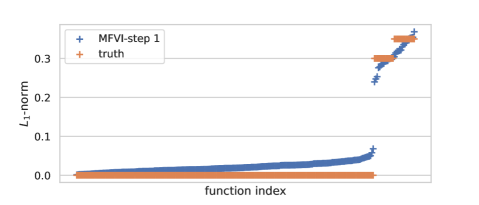
Figure 1: Estimated $L_{1}$-norms $(\hat{S}_{(i)})_{i\in[K^{2}]}$ (blue dots), based on the mean-field adaptive variational posterior mean and the set of models $\mathcal{M}_{C}$ containing models with complete graph $\delta_{C}=\mathds{1}\mathds{1}^{T}$, plotted in increasing order. The orange dots correspond to the true values $S_{lk}^{0}=\|h_{lk}^{0}\|_{1}$. These results correspond to one realisation of the Excitation scenario of Simulation 4, for the Hawkes processes with $K=16$ dimensions.

Therefore, once $\hat{\delta}$ is obtained, we compute an adaptive variational Bayes posterior, conditional on $\delta=\hat{\delta}$, by considering the set of models

$$\mathcal{M}_{E}:=\{m=(\hat{\delta},J=(J_{k})_{k});\>J_{k}\geqslant 1,\>\forall k\in[K]\}.$$ (17)

In summary, our adaptive two-step algorithm writes as:

1. Complete graph VB:

   (a) compute the VB posterior associated to the set of models $\mathcal{M}_{C}$, i.e., to the complete graph $\delta_{C}=\mathds{1}\mathds{1}^{T}$, and compute the posterior mean of $S_{lk}=\|h_{lk}\|_{1}$, denoted $\hat{S}_{lk}$, $\forall(l,k)\in[K]^{2}$.

   (b) order the values $\hat{S}_{lk}$ in increasing order, say $\hat{S}_{(1)}\leqslant\hat{S}_{(2)}\leqslant\cdots\leqslant\tilde{S}_{(K^{2})}$, and define $\hat{\delta}_{lk}=1$ iff $\hat{S}_{lk}>\eta_{0}$, where $\eta_{0}$ is a threshold defined by the first significant value of $\hat{S}_{(i+1)}-\hat{S}_{(i)}$.

2. Graph-restricted VB: compute the VB posterior associated to the set of models $\mathcal{M}_{E}$, i.e., to models with $\delta=\hat{\delta}$.

Theoretical validation of our procedure is provided in Section 4.1. We also note that different variants of our two-step strategy are possible. In particular one can choose a different threshold for each dimension $k\in[K]$, since different convergence rates could be obtained in the different dimensions. Moreover, one can potentially remove the model selection procedure to choose the $J_{k}$’s, $k\in[K]$ in the first step 1(a), and compute a variational posterior in only one model $m\in\mathcal{M}_{C}$.

In the next section we consider the case of the sigmoid Hawkes processes, for which a data augmentation scheme allows to efficiently compute a mean-field approximation of the posterior distribution within a model $m$.

Remark 2

In recent work, Bonnet et al. (2021) also propose a thresholding approach for estimating the connectivity graph $\delta$ in the context of parametric maximum likelihood estimation. In fact, an alternative strategy to our procedure derived from their work would consist in defining the graph estimator as $\hat{\delta}_{lk}=1\iff\tilde{S}_{lk}>\varepsilon\sum_{l,k}\tilde{S}_{lk}$, where $\varepsilon\in(0,1)$ is a pre-defined or data-driven threshold.

3 Adaptive variational Bayes algorithms in the sigmoid model

In this section, we focus on the sigmoid Hawkes model, for which the link functions in (1) are sigmoid-type functions. We consider the following parametrisation of this model: for each $k\in[K]$,

$$\phi_{k}(x)=\theta_{k}\tilde{\sigma}(x),\quad\tilde{\sigma}(x)=\sigma\left(\alpha(x-\eta)\right),\quad\sigma(x):=(1+e^{-x})^{-1},\quad\alpha>0,\>\eta>0,\>\theta_{k}>0.$$ (18)

Here, we assume that the hyperparameters $\alpha,\eta$ and $\theta=(\theta_{k})_{k}$ are known; however, our methodology can be directly extended to estimate an unknown $\theta$, similarly to Zhou et al. (2022) and Malem-Shinitski et al. (2021). We first note that for $\alpha=0.1,\eta=10$ and $\theta_{k}=20$, the nonlinearity $\phi_{k}$ is similar to the ReLU and softplus functions on $[-\infty,20]$ (see Figure 2 in Section 5). This is helpful to compare the impact of the link functions on the inference in our numerical experiments in Section 5.

For sigmoid-type of link functions, efficient mean-field variational inference methods based on data augmentation and Gaussian priors have been previously proposed, notably by Malem-Shinitski et al. (2021); Zhou et al. (2021a, 2022). We first recall this latent variable augmentation scheme, which allows to obtain a conjugate form for the variational posterior distribution in a fixed model $m=(\delta,J)$ (see Section 2.1). Then, building on this prior work, we provide two explicit algorithms based on the adaptive and sparsity-inducing methodology presented in Section 2.3.

3.1 Augmented mean-field variational inference in a fixed model

In our method, we leverage existing latent variable augmentation strategy and Gaussian prior construction, which allows to efficiently compute a mean-field variational posterior distribution on $\mathcal{F}_{m}\subset\mathcal{F}$, the parameter subspace within a model $m=(\delta,J_{lk};(l,k)\in\mathcal{I}(\delta))$. The details of this construction are provided in Appendix B and we recall that in this context, the set of latent variables $\omega,\bar{Z}$ correspond respectively to marks at each point of the point process $N$ and to a marked Poisson point process on $[0,T]\times\varmathbb R^{+}$.

Then, the augmented mean-field variational family (9) approximating the augmented posterior distribution corresponds to

$$\mathcal{V}_{AMF}=\left\{Q:\mathcal{F}\times\mathcal{O}\times\mathcal{Z}\to\varmathbb R^{+};\>dQ(f,\omega,\bar{Z})=dQ_{1}(f)dQ_{2}(\omega,\bar{Z})\right\},$$

where $\mathcal{O}$ and $\mathcal{Z}$ denote the latent variable spaces. More precisely, in our method, we use the mean-field approach within a fixed model $m$, and therefore define the model-restricted mean-field variational class as

$$\mathcal{V}_{AMF}^{m}=\left\{Q:\mathcal{F}_{m}\times\mathcal{O}\times\mathcal{Z};\>dQ(f,\omega,\bar{Z})=dQ_{1}(f)dQ_{2}(\omega,\bar{Z})\right\},$$

leading to the model-restricted variational posterior $\hat{Q}_{AMF}^{m}(f,\omega,\bar{Z})=\hat{Q}_{1}^{m}(f)\hat{Q}_{2}^{m}(\omega,\bar{Z})$.

Then, we introduce a family of Gaussian prior distributions $\Pi_{h|\delta,J}(h)$ on $\mathcal{F}_{m}$ such that the factors of $\hat{Q}_{AMF}^{m}$, $\hat{Q}_{1}^{m}$ and $\hat{Q}_{2}^{m}$, are conjugate. This conjugacy leads to an iterative variational inference algorithms with closed-forms updates, using (33). Let $|J|=\sum_{k}J_{k}$. We define

$$\mathcal{H}_{e}^{J}=\left\{h=(h_{lk})_{l,k}\in\mathcal{H};\>h_{lk}(x)=\sum_{j=1}^{J_{k}}h^{j}_{lk}e_{j}(x),\>x\in[0,A],\>\underline{h}_{lk}^{J_{k}}=(h_{lk}^{1},\dots,h_{lk}^{J_{k}})\in\varmathbb R^{J_{k}},\>\forall(l,k)\in[K]^{2}\right\}.$$

Now, for each $(l,k)$, if $\delta_{lk}=1$, we consider a normal prior distribution on $\underline{h}_{lk}^{J_{k}}$, with mean vector $\mu_{J_{k}}\in\varmathbb R^{J_{k}}$ and covariance matrix $\Sigma_{J_{k}}\in\varmathbb R^{J_{k}\times J_{k}}$, i.e., $\underline{h}_{lk}^{J_{k}}\sim\mathcal{N}(\mu_{J_{k}},\Sigma_{J_{k}})$, and if $\delta_{lk}=0$, we set $\underline{h}_{lk}^{J_{k}}=\mathbf{0}_{J_{k}}$. We then denote $\mu_{m}=(\mu_{k}^{m})_{k}$ with $\mu_{k}^{m}=(\delta_{lk}\mu_{J_{k}})_{l}\in\varmathbb R^{KJ_{k}}$ and $\Sigma_{m}=Diag((\Sigma_{k}^{m})_{k})$ with $\Sigma_{k}^{m}=Diag((\delta_{lk}\Sigma_{J_{k}})_{l})\in\varmathbb R^{KJ_{k}\times KJ_{k}}$. We also consider a normal prior on the background rates, i.e., $\nu_{k}\overset{i.i.d}{\sim}\mathcal{N}(\mu_{\nu},\sigma_{\nu}^{2})$ with hyperparameters $\mu_{\nu},\sigma_{\nu}>0$. We finally denote by $f_{m}:=(f_{k}^{m})_{k}\in\mathcal{F}_{m}$ where for each $k$, $f_{k}^{m}=(\nu_{k},\underline{h}_{1k}^{J_{k}},\dots,\underline{h}_{Kk}^{J_{k}})\in\varmathbb R^{KJ_{k}+1}$, and define $H(t)=(H^{0}(t),H^{1}(t),\dots,H^{K}(t))\in\varmathbb R^{|J|+1}$, where $H_{0}(t)=1$ and for $k\in[K]$, $H^{k}(t)=(H_{j}^{k}(t))_{j=1,\dots,J_{k}}$ with

$$H_{j}^{k}(t):=\int_{t-A}^{t}e_{j}(t-s)dN^{k}_{s},\quad j\in[J_{k}].$$ (19)

Using similar computations as in Donner and Opper (2019); Zhou et al. (2021a); Malem-Shinitski et al. (2021), we can derive analytic forms for $\hat{Q}_{1}^{m}$ and $\hat{Q}_{2}^{m}$. In particular, we have that $\hat{Q}_{1}^{m}(f_{m})=\prod_{k}\hat{Q}_{1}^{m,k}(f_{k}^{m})$, and for each $k$, $\hat{Q}_{1}^{m,k}(f_{k}^{m})$ is a normal distribution with mean vector $\tilde{\mu}_{k}^{m}\in\varmathbb R^{KJ_{k}+1}$ and covariance matrix $\tilde{\Sigma}_{k}^{m}\in\varmathbb R^{(KJ_{k}+1)\times(KJ_{k}+1)}$ given by

$$\tilde{\Sigma}_{k}^{m} =\left[\alpha^{2}\sum_{i\in[N_{k}]}\varmathbb{E}_{\hat{Q}_{2}^{m,k}}[\omega_{i}^{k}]H(T_{i}^{k})H(T_{i}^{k})^{T}+\alpha^{2}\int_{0}^{T}\int_{0}^{+\infty}\bar{\omega}_{t}^{k}H(t)H(t)^{T}\Lambda^{k}(t,\bar{\omega})d\bar{\omega}dt+(\Sigma_{k}^{m})^{-1}\right]^{-1},$$ (20)

$$\tilde{\mu}_{k}^{m} =\frac{1}{2}\tilde{\Sigma}_{k}^{m}\left[\alpha\sum_{i\in[N_{k}]}(2\varmathbb{E}_{\hat{Q}_{2s}^{k}}[\omega_{i}^{k}]\alpha\eta+1)H(T_{i}^{k})+\alpha\int_{0}^{T}\int_{0}^{+\infty}\left(2\bar{\omega}^{k}\alpha\eta-1\right)H(t)\Lambda^{k}(t,\bar{\omega})d\bar{\omega}dt+2(\Sigma_{k}^{m})^{-1}\mu_{k}^{m}\right],$$ (21)

where $N_{k}:=N^{k}[0,T]$ and

$$\Lambda^{k}(t,\bar{\omega}):=\theta_{k}\frac{\exp\left\{-\frac{1}{2}\varmathbb{E}_{Q_{1}^{m,k}}[\tilde{\lambda}^{k}_{t}(f_{k}^{s})]\right\}}{2\cosh\frac{c^{k}_{t}}{2}}p_{PG}(\bar{\omega};1,c^{k}_{t}),\quad c^{k}_{t}:=\sqrt{\varmathbb{E}_{Q_{1}^{m,k}}[\tilde{\lambda}^{k}_{t}(f)^{2}]}.$$

Besides, we also have that $\hat{Q}_{2}^{m}(\omega,\bar{Z})=\hat{Q}_{21}^{m}(\omega)\hat{Q}_{22}^{m}(\bar{Z})$ with $\hat{Q}_{21}^{m}(\omega)=\prod_{k}\prod_{i\in[N_{k}]}p_{PG}(\omega_{i}^{k};1,c^{k}_{T_{i}^{k}})$ and $\hat{Q}_{22}^{m}=\prod_{k}\hat{Q}^{m,k}_{22}$ where for each $k$, $\hat{Q}^{m,k}_{22}$ is the probability distribution of a marked Poisson point process on $[0,T]\times\varmathbb R^{+}$ with intensity measure $\Lambda^{k}(t,\bar{\omega})$. The full derivation of these formulas can be found in Appendix C.1.

From the previous expression, we can compute $\hat{Q}_{2}^{m}$ given an estimate of $\hat{Q}_{1}^{m}$, and conversely. Therefore, to compute the model-restricted mean-field variational posterior $\hat{Q}^{m}$, we use an iterative algorithm that updates each factor alternatively, a procedure summarised in Algorithm 1. We note that the updates of the mean vectors and covariance matrices require to compute an integral, which we perform using the Gaussian quadrature method (Golub and Welsch, 1969), where the number of points, denoted $n_{GQ}$, is a hyperparameter of our method. We finally recall that in this algorithm, each variational factor $\hat{Q}_{k}^{m}$ can be computed independently and only depends on a subset of the parameter $f_{k}$, and hence, of the sub-model, $m_{k}:=(\delta_{k},J_{k})$.

Remark 3

The number of iterations $n_{iter}$ in Algorithm 1 is another hyperparameter of our method. In practice, we implement an early-stopping procedure, where we set a maximum number of iterations, such as 100, and stop the algorithm whenever the increase of the ELBO is small, e.g., lower than $10^{-3}$, indicating that the algorithm has converged.

Remark 4

Similarly to Zhou et al. (2021a); Malem-Shinitski et al. (2021), we can also derive analytic forms of the conditional distributions of the augmented posterior (40). Therefore, the latter could be computed via a Gibbs sampler, which is provided in Algorithm 4 in Appendix C.3. However, in this Gibbs sampler, one needs to sample the latent variables - in particular a $K$-dimensional inhomogeneous Poisson point process. This is therefore computationally much slower than the variational inference counterpart, which only implies to compute expectation wrt to the latent variables distribution.

Input: $N=(N^{1},\dots,N^{K})$, $m=(\delta,J),\>J=(J_{1},\dots,J_{K})$, $\mu_{m}=(\mu_{k}^{m})_{k},\Sigma_{m}=(\Sigma_{k}^{m})_{k}$, $n_{iter}$, $n_{GQ}$.

Output: $\tilde{\mu}_{m}=(\tilde{\mu}_{k}^{m})_{k},\tilde{\Sigma}_{m}=(\tilde{\Sigma}_{k}^{m})_{k}$.

1 Precompute $(H(T_{i}^{k}))_{i,k}$.

2 Precompute $(p_{q},v_{q})_{q\in[n_{GQ}]}$ (points and weights for Gaussian quadrature) and $(H(p_{q}))_{q\in[n_{GQ}]}$ .

3 do in parallel for each $k=1,\dots,K$

4       Initialisation: $\tilde{\mu}_{k}^{m}\leftarrow\mu_{k}^{m}$, $\tilde{\Sigma}_{k}^{m}\leftarrow\Sigma_{k}^{m}$.

5       for $t\leftarrow 1$ to $n_{iter}$ do

6             for $i\leftarrow 1$ to $N_{k}$ do

7                   $\varmathbb{E}_{\hat{Q}_{1}^{m,k}}[\tilde{\lambda}^{k}_{T_{i}^{k}}(f_{k}^{m})^{2}]=\alpha\left(H(T_{i}^{k})^{T}\tilde{\Sigma}_{k}^{s}H(T_{i}^{k})+(H(T_{i}^{k})^{T}\tilde{\mu}_{k}^{s})^{2}-2\eta H(T_{i}^{k})^{T}\tilde{\mu}_{k}^{m}+\eta^{2}\right)$

8                   $\varmathbb{E}_{\hat{Q}_{2}^{m,k}}[\omega_{i}^{k}]=\tanh\left(\sqrt{\varmathbb{E}_{\hat{Q}_{1}^{m,k}}[\tilde{\lambda}^{k}_{T_{i}^{k}}(f_{k}^{s})^{2}]}\right)/\left(2\sqrt{\varmathbb{E}_{\hat{Q}_{1}^{m,k}}[\tilde{\lambda}^{k}_{T_{i}^{k}}(f_{k}^{m})^{2}]}\right)$

9            for $q\leftarrow 1$ to $n_{GQ}$ do

10                   $\varmathbb{E}_{\hat{Q}_{1}^{m,k}}[\tilde{\lambda}_{p_{q}}^{k}(f_{k}^{m})^{2}]=\alpha\left(H(p_{q})^{T}\tilde{\Sigma}_{k}^{m}H(p_{q})+(H(p_{q})^{T}\tilde{\mu}_{k}^{m})^{2}-2\eta H(p_{q})^{T}\tilde{\mu}_{k}^{m}+\eta^{2}\right)$

11                   $\varmathbb{E}_{\hat{Q}_{2}^{m,k}}[\omega_{q}^{k}]=\tanh\left(\sqrt{\varmathbb{E}_{\hat{Q}_{1}^{m,k}}[\tilde{\lambda}^{k}_{p_{q}}(f_{k}^{s})^{2}]}\right)/\left(2\sqrt{\varmathbb{E}_{\hat{Q}_{1}^{m,k}}[\tilde{\lambda}^{k}_{p_{q}}(f_{k}^{m})^{2}]}\right)$

12                   $\varmathbb{E}_{\hat{Q}_{1}^{m,k}}[\tilde{\lambda}_{p_{q}}^{k}(f_{k}^{m})]=\alpha\left((\tilde{\mu}_{k}^{m})^{T}H(p_{q})-\eta\right)$

13                  

14            Compute $\tilde{\Sigma}_{k}^{m}$ and $\tilde{\mu}_{k}^{m}$ using (20) and (21)

15      

16

Algorithm 1 Mean-field variational inference algorithm in a fixed model

3.2 Adaptive variational algorithms

Using Algorithm 1 for computing a model-restricted mean-field variational posterior, we now leverage the model-selection and two-step approach from Section 2.1 to design two adaptive variational Bayes algorithms. The first one, denoted fully-adaptive, is only based on the model-selection strategy from Section 2.2 and is suitable for low-dimensional settings. The second one, denoted two-step adaptive, relies on a partial model-selection strategy and the two-step approach from Section 2.3, and is more efficient for moderately large to large dimensions of the point process.

3.2.1 Fully-adaptive variational algorithm

From now on, we assume that the number of functions $(e_{j})$ in the dictionary is bounded by $J_{T}\in\varmathbb{N}$. We then define the set of models

$$\mathcal{M}_{T}=\big{\{}m=(\delta,J=(J_{k})_{k});\>\delta\in\{0,1\}^{K\times K},\>1\leqslant J_{k}\leqslant J_{T},\>k\in[K]\big{\}}.$$ (22)

We can easily see that in this case $|\mathcal{M}_{T}|\sim 2^{K^{2}}J_{T}$, and that for any $m=(\delta,J)\in\mathcal{M}_{T}$, the number of parameters in $m$ is equal to $\sum_{l,k}\delta_{lk}(J_{k}+1)+1$. Therefore, we recall that exploring all models in $\mathcal{M}_{T}$ is only computationally feasible for low-dimensional settings, e.g., $K\leqslant 3$. We also recall our notation $m=(m_{k})_{k}$ with $m_{k}=(\delta_{\cdot k},J_{k}),\forall k$.

Let $\Pi_{m}$ be a prior distribution on $\mathcal{M}_{T}$ of the form

$$\Pi_{m}(m)=\prod_{k}\Pi_{m}(m_{k})=\prod_{k}\Pi_{k,\delta}(\delta_{\cdot k})\Pi_{k,J}(J_{k}).$$

For instance, one can choose $\Pi_{k,\delta}$ as a product of Bernoulli distribution with parameter $p\in(0,1)$ and $\Pi_{k,J}$ as the uniform distribution over $[J_{T}]$. Using Algorithm 1, for each $m=(m_{k})_{k}$, we compute $\hat{Q}_{k}^{m}$ together with the corresponding $ELBO(\hat{Q}_{k}^{m})$ for each $k$. We note that the computations for each model can be computed independently, and therefore be parallelised to further accelerate posterior inference.

Then, we recall that the model-selection adaptive variational approach consists in either selecting $\hat{m}$ which maximises the ELBO over $m\in\mathcal{M}_{T}$ (see (12)) or in averaging over the different models $m$ (see (13)). In the first case, with $\hat{m}_{k}=\arg\max_{m_{k}}ELBO(\hat{Q}_{k}^{m})$, the VB posterior is $\hat{Q}_{MS}=\otimes_{k=1}^{K}\hat{Q}_{k}^{\hat{m}_{k}}$. In the second case, the model-averaging adaptive variational posterior is given by

$$\hat{Q}_{AV}=\otimes_{k=1}^{K}\hat{Q}_{k}^{AV},\quad\hat{Q}^{AV}_{k}=\sum_{m_{k}}\hat{\gamma}_{k}^{m}\hat{Q}_{k}^{m},\quad\hat{\gamma}_{k}^{m}=\frac{\tilde{\gamma}_{k}^{m}}{\sum_{m}\tilde{\gamma}_{k}^{m}}$$

$$\tilde{\gamma}_{k}^{m}=\Pi_{k,\delta}(\delta_{\cdot k})\Pi_{k,J}(J_{k})\exp\left\{ELBO(\hat{Q}_{k}^{m})\right\}.$$ (23)

We call this procedure (exploring all models in $\mathcal{M}_{T}$) the fully-adaptive mean-field variational inference algorithm, and summarise its steps in Algorithm 2. In the next section, we propose a faster algorithm that avoids the exploration of all models in $\mathcal{M}_{T}$.

Input: $N=(N^{1},\dots,N^{K})$, $\mathcal{M}_{T}$, $\mu=(\mu_{m})_{m\in\mathcal{M}_{T}},\Sigma=(\Sigma_{m})_{m\in\mathcal{M}_{T}}$, $n_{iter}$, $n_{GQ}$.

Output: $\hat{Q}_{AV}$ or $\hat{Q}_{MV}$.

1 do in parallel for each $m=(\delta,D)\in\mathcal{M}_{T}$

2       Compute the variational posterior $\hat{Q}_{m}$ using Algorithm 1 with $\mu_{m},\Sigma_{m}$, $n_{iter}$ and $n_{GQ}$ as hyperparameters.

3       Compute $(ELBO(\hat{Q}_{k}^{m})_{k})$ and $(\tilde{\gamma}_{k}^{m})_{k}$ using (23).

4

Compute $\{\hat{\gamma}_{m}\}_{m\in\mathcal{M}_{T}}$ and $\hat{Q}_{AV}$ or $\hat{Q}_{MS}$.

Algorithm 2 Fully-adaptive mean-field variational inference

3.2.2 Two-step adaptive mean-field algorithm

As discussed in the above section, for moderately large values of $K$, the model-averaging or model-selection procedures in Algorithm 2 become prohibitive. In this case, we instead use the two-step approach introduced in Section 2.3.

We recall that this strategy corresponds to starting with a maximal graph $\delta_{C}$, typically the complete graph $\delta_{C}=\mathds{1}\mathds{1}^{T}$, and considering the set of models $\mathcal{M}_{C}=\big{\{}m=(\delta_{C},J=(J_{k})_{k});\>1\leqslant J_{k}\leqslant J_{T},\>k\in[K]\big{\}},$ where here as well we assume that the number of functions in the dictionary is bounded by $J_{T}$. Then, after computing a graph estimator $\hat{\delta}$, we consider the second set of models $\mathcal{M}_{E}=\big{\{}m=(\hat{\delta},J=(J_{k})_{k});\>1\leqslant J_{k}\leqslant J_{T},\>k\in[K]\big{\}}$. We note that both $\mathcal{M}_{C}$ and $\mathcal{M}_{E}$ have cardinality of order $KJ_{T}$, and the cardinality of models per dimension is $J_{T}$. Therefore, as soon as the computation for each model is fast and $J_{T}$ is not too large, optimisation procedures over these two sets are feasible, even for large values of $K$.

In the first step of our fast algorithm, we compute the model-selection adaptive VB posterior $\hat{Q}_{MS}^{C}$ using Algorithm 2, replacing $\mathcal{M}_{T}$ by $\mathcal{M}_{C}$. Then, we use $\hat{Q}_{MS}^{C}$ to estimate the norms $(\left\lVert h_{lk}\right\rVert_{1})_{l,k}$ and the graph parameter, with the thresholding method described in Section 2.3:
(a) denoting $\hat{J}_{C}=(J_{k,C})_{k}$ the selected dimensionality in $\hat{Q}_{MS}^{C}$, we compute our estimates of the norm $\hat{S}_{lk}=\varmathbb{E}_{\hat{Q}_{MS}^{C}}[\left\lVert h_{lk}\right\rVert_{1}],\>\forall(l,k)$, and define $\hat{S}=(\hat{S}_{lk})_{l,k}\in\varmathbb R_{+}^{K\times K}$;
(b) we order our estimates $\hat{S}_{(1)}<\dots<\hat{S}_{(K^{2})}$ and choose a threshold $\eta_{0}$ in the first significant gap between $\hat{S}_{(i)}$ and $\hat{S}_{(i+1)}$, $i\in[K^{2}]$;
(c) we compute the graph estimator $\hat{\delta}=(\hat{\delta}_{lk})_{l,k}$ defined for any $k$ and $l$ by $\hat{\delta}_{lk}=\mathds{1}_{\{\hat{S}_{lk}>\eta_{0}\}}.$

In the second step, we compute the adaptive model-selection VB posterior $\hat{Q}_{MS}$ or model-averaging VB posterior $\hat{Q}_{AV}$ using Algorithm 2, replacing $\mathcal{M}_{T}$ by $\mathcal{M}_{E}$.

This procedure is summarised in Algorithm 3. In the next section, we provide theoretical guarantees for general variational Bayes approaches, and apply them to our adaptive and mean-field algorithms.

Input: $N=(N^{1},\dots,N^{K})$, $\mathcal{M}_{T}$, $\mu=(\mu_{m})_{m},\Sigma=(\Sigma_{m})_{m}$, $n_{iter}$, $n_{GQ}$.

Output: $\hat{Q}_{MS}$ or $\hat{Q}_{AV}$

Compute $\hat{Q}_{MS}$ using Algorithm 2 with input set $\mathcal{M}_{C}$ and hyperparameters $\mu=(\mu_{m})_{m},\Sigma=(\Sigma_{m})_{m}$, $n_{iter}$, $n_{GQ}$. Compute $\hat{\delta}$ using the thresholding of the estimate $\tilde{S}$. Compute $\hat{Q}_{MS}^{C}$ or $\hat{Q}_{AV}$ using Algorithm 2 with input set $\mathcal{M}_{E}$ and hyperparameters $\mu=(\mu_{m})_{m},\Sigma=(\Sigma_{m})_{m}$, $n_{iter}$, $n_{GQ}$.

Algorithm 3 Two-step adaptive mean-field variational inference

4 Theoretical properties of the variational posteriors

This section contains general results on variational Bayes methods for estimating the parameter of Hawkes processes, and theoretical guarantees for our adaptive and mean-field approaches proposed in Section 2 and Section 3. In particular, we derive the concentration rates of variational Bayes posterior distributions, under general conditions on the model, the prior distribution, and the variational family. Then, we apply our general result to variational methods of practical interest, in particular our model-selection adaptive and mean-field methods.

We recall that in our problem setting, the link functions $\phi:=(\phi_{k})_{k}$ in the nonlinear intensity (1) are fixed by the statistician and therefore known a-priori. Throughout the section we assume that these functions are monotone non-decreasing, $L$-Lipschitz, $L>0$, and that one of the two following conditions is satisfied:

• For a parameter $f=(\nu,h)$, the matrix defined by $S^{+}=(S^{+}_{lk})_{l,k}\in\varmathbb R_{+}^{K\times K}$ with $S_{lk}^{+}=L\left\lVert h_{lk}^{+}\right\rVert_{1},\forall l,k$, satisfies $\left\lVert S^{+}\right\rVert<1$;

• For any $k\in[K]$, the link function $\phi_{k}$ is bounded, i.e., $\exists\Lambda_{k}>0,\forall x\in\varmathbb R$, $0\leqslant\phi_{k}(x)\leqslant\Lambda_{k}$.

These conditions are sufficient to prove that the Hawkes process is stationary (see for instance Bremaud and Massoulie (1996), Deutsch and Ross (2022), or Sulem et al. (2021)).

4.1 Variational posterior concentration rates

To establish our general concentration result on the VB posterior distribution, we need to introduce the following assumption, also used to prove the concentration of the posterior distribution (4) in the nonlinear Hawkes model in Sulem et al. (2021).

Assumption 5

For a parameter $f$, we assume that there exists $\varepsilon>0$ such that for each $k\in[K]$, the link function $\phi_{k}$ restricted to $I_{k}=(\nu_{k}-\max\limits_{l\in[K]}\left\lVert h_{lk}^{-}\right\rVert_{\infty}-\varepsilon,\nu_{k}+\max\limits_{l\in[K]}\left\lVert h_{lk}^{+}\right\rVert_{\infty}+\varepsilon)$ is bijective from $I_{k}$ to $J_{k}=\phi_{k}(I_{k})$ and its inverse is $L^{\prime}$- Lipschitz on $J_{k}$, with $L^{\prime}>0$. We also assume that at least one of the two following conditions is satisfied.

1. For any $k\in[K]$, $\inf\limits_{x\in\varmathbb R}\phi_{k}(x)>0$.

2. For any $k\in[K]$, $\phi_{k}>0$, and $\sqrt{\phi_{k}}$ and $\log\phi_{k}$ are $L_{1}$-Lipschitz with $L_{1}>0$ .

In Sulem et al. (2021), Assumption 5 is used to obtain general posterior concentration rates, and is verified for commonly used link functions (see Example 1 in Sulem et al. (2021)). In particular, it holds for sigmoid-type link functions, such as the ones considered in Section 3, when the parameter space is bounded (see below).

We now define our parameter space $\mathcal{F}$ as follows

$$\mathcal{H}^{\prime}=\left\{h:[0,A]\to\varmathbb R;\>\|h\|_{\infty}<\infty\right\},\quad\mathcal{H}=\left\{h=(h_{lk})_{l,k=1}^{K}\in\mathcal{H}^{\prime K^{2}};\>(h,\phi)\text{ satisfy {(C1)} or {(C2)} }\right\},$$

$$\mathcal{F}=\left\{f=(\nu,h)\in(\varmathbb R_{+}\backslash\{0\})^{K}\times\mathcal{H};\>(f,\phi)\text{ satisfies Assumption \leavevmode\nobreak\ \ref{ass-psi} }\right\}.$$

We also define the $L_{1}$-distance for any $f,f^{\prime}\in\mathcal{F}$ as

$$\|f-f^{\prime}\|_{1}:=\left\lVert\nu-\nu^{\prime}\right\rVert_{1}+\left\lVert h-h^{\prime}\right\rVert_{1},\quad\left\lVert h-h^{\prime}\right\rVert_{1}:=\sum_{l,k=1}^{K}\left\lVert h_{lk}-h_{lk}^{\prime}\right\rVert_{1},\quad\left\lVert\nu-\nu^{\prime}\right\rVert_{1}:=\sum_{k}|\nu_{k}-\nu_{k}^{\prime}|.$$

In particular, for the sigmoid function $\phi_{k}(x)=\theta_{k}\sigma(\alpha(x-\eta))$, we can choose $\mathcal{F}=\left\{f=(\nu,h)\in[0,B]^{K}\times\mathcal{H}\right\}$, with $B>0$. Moreover, we introduce

$$B_{\infty}(\epsilon)=\left\{f\in\mathcal{F};\>\nu_{k}^{0}\leqslant\nu_{k}\leqslant\nu_{k}^{0}+\epsilon,\,h_{lk}^{0}\leqslant h_{lk}\leqslant h_{lk}^{0}+\epsilon,\>(l,k)\in[K]^{2}\right\},\quad\epsilon>0,$$

a neighbourhood around $f_{0}$ in supremum norm, and a sequence $(\kappa_{T})_{T}$ defined as

$$\kappa_{T}:=10(\log T)^{r},$$ (24)

with $r=0$ if $(\phi_{k})_{k}$ satisfies Assumption 5 (i), and $r=1$ if $(\phi_{k})_{k}$ satisfies Assumption 5 (ii). We can now state our general theorem.

Theorem 6

Let $N$ be a Hawkes process with link functions $\phi=(\phi_{k})_{k}$ and parameter $f_{0}=(\nu_{0},h_{0})$ such that $(\phi,f_{0})$ satisfy Assumption 5 and (C1) or (C2). Let $\epsilon_{T}=o(1/\sqrt{\kappa_{T}})$ be a positive sequence verifying $\log^{3}T=O(T\epsilon_{T}^{2})$, $\Pi$ a prior distribution on $\mathcal{F}$ and $\mathcal{V}$ a variational family of distributions on $\mathcal{F}$. We assume that the following conditions are satisfied for $T$ large enough.

(A0) There exists $c_{1}>0$ such that $\Pi(B_{\infty}(\epsilon_{T}))\geqslant e^{-c_{1}T\epsilon_{T}^{2}}.$

(A1) There exist $\mathcal{H}_{T}\subset\mathcal{H}$, $\zeta_{0}>0$, and $x_{0}>0$ such that

$$\Pi(\mathcal{H}_{T}^{c})=o(e^{-(\kappa_{T}+c_{1})T\epsilon_{T}^{2}})\quad\mbox{and}\quad\log\mathcal{N}\left(\zeta_{0}\epsilon_{T},\mathcal{H}_{T},||\cdot||_{1}\right)\leqslant x_{0}T\epsilon_{T}^{2}.$$

(A2) There exists $Q\in\mathcal{V}$ such that $supp(Q)\subset B_{\infty}(\epsilon_{T})$ and $KL(Q||\Pi)=O(\kappa_{T}T\epsilon_{T}^{2}).$

Then, for any $M_{T}\to\infty$ and $\hat{Q}$ defined in (8), we have that

$$\varmathbb{E}_{0}\left[\hat{Q}\left(\left\lVert f-f_{0}\right\rVert_{1}>M_{T}\sqrt{\kappa_{T}}\epsilon_{T}\right)\right]\xrightarrow[T\to\infty]{}0.$$

The proof of Theorem 6 is reported in Appendix D.2 and leverage existing theory on posterior concentration rates. We now make a few remarks related to the previous results.

Firstly, similarly to Donnet et al. (2020) Sulem et al. (2021), Theorem 6 also holds when the neighborhoods $B_{\infty}(\epsilon_{T})$ around $f_{0}$ in supremum norm, considered in Assumptions (A0) and (A2), are replaced neighborhoods in $L_{2}$-norm, defined as

$$B_{2}(\epsilon_{T},B)=\left\{f\in\mathcal{F};\>\max_{k}|\nu_{k}-\nu_{k}^{0}|\leqslant\epsilon_{T},\>\max_{l,k}\|h_{lk}-h_{lk}^{0}\|_{2}\leqslant\epsilon_{T},\>\max_{l}\nu_{l}+\max_{k}\|h_{kl}\|_{\infty}<B\right\},$$

with $B>0$, and when $\kappa_{T}$ replaced by $\kappa_{T}^{\prime}=10(\log\log T)(\log T)^{r}$.

Secondly, Theorem 6 also holds under the more general condition on the variational family:
    (A2’) The variational family $\mathcal{V}$ verifies $\min_{Q\in\mathcal{V}}KL(Q||\Pi(.|N))=O(\kappa_{T}T\epsilon_{T}^{2}).$ However, in practice, one often verifies (A2) and deduces (A2’) using the following steps from Zhang and Gao (2020). For any $Q\in\mathcal{V}$, we have that

$$KL(Q||\Pi(.|N))\leqslant KL(Q||\Pi)+Q(KL(\varmathbb{P}_{T,f_{0}},\varmathbb{P}_{T,f})),$$

where we denote $\varmathbb{P}_{T,f_{0}}=e^{L_{T}(f_{0})}$ and $\varmathbb{P}_{T,f}=e^{L_{T}(f)}$. Using Lemma S6.1 from Sulem et al. (2021), for any $f\in B_{\infty}(\epsilon_{T})$, we also have that

$$\varmathbb{E}_{0}\left[L_{T}(f_{0})-L_{T}(f)\right]\leqslant\kappa_{T}T\epsilon_{T}^{2}.$$

Therefore, under (A2), there exists $Q\in\mathcal{V}$ such that $KL(Q||\Pi(.|N))=O(\kappa_{T}T\epsilon_{T}^{2}),$ which implies (A2’) . Besides, (A2) (or (A2’)), is the only condition on the variational class, and informally states that this family of distributions can approximate the true posterior conveniently. Nonetheless, under (A2), we may still have $\min_{Q\in\mathcal{V}}KL(Q||\Pi(.|N))\xrightarrow[T\to\infty]{}\infty$, as has been observed by Nieman et al. (2021).

Finally, Assumptions (A0) and (A1) are similar to the ones of Theorem 3.2 in Sulem et al. (2021). They are sufficient conditions for proving that the posterior concentration rate is at least as fast as $\sqrt{\kappa_{T}}\epsilon_{T}$.

4.2 Applications to variational classes and prior families of interest

In this section, we apply the previous result to variational inference methods of interest in nonlinear Hawkes models, in particular, the mean-field and model-selection variational families, introduced in Section 2.2 and used in our algorithms. We also verify our general conditions on the prior distribution on two common examples of nonparametric prior families, namely random histograms and Gaussian processes, see for instance in Donnet et al. (2020); Malem-Shinitski et al. (2021). We then obtain explicit concentration rates for the variational posterior distribution and for Hölder classes of functions.

First, we re-write our hierarchical spike-and-slab prior distribution from Section 2.1 as

$$d\Pi(f)=d\Pi_{\nu}(\nu)d\Pi_{\delta}(\delta)d\Pi_{h|\delta}(h),\quad d\Pi_{h|\delta}(h)=\prod_{l,k}d\tilde{\Pi}_{h|\delta}(h_{lk})$$ (25)

and recall that from Sulem et al. (2021), we know that Assumption (A0) of Theorem 6 can be replaced by

(A0’) There exists $c_{1}>0$ such that $\Pi(B_{\infty}(\epsilon_{T})|\delta=\delta_{0})\geqslant e^{-c_{1}T\epsilon_{T}^{2}/2}$ and $\Pi_{\delta}(\delta=\delta_{0})\geqslant e^{-c_{1}T\epsilon_{T}^{2}/2}$.

Furthermore, one can choose for instance $\Pi_{\delta}=\mathcal{B}(p)^{K^{2}}$ with $p\in(0,1)$, implying that the $\delta_{lk}$’s are i.i.d. Bernoulli random variables. Then, for any fixed $p$, one only needs to verify $\Pi_{h|\delta}(B_{\infty}(\epsilon_{T})|\delta=\delta_{0})\geqslant e^{-c_{1}T\epsilon_{T}^{2}/2}$.

4.2.1 Mean-field variational family

Here, we consider the mean-field variational inference method with general latent variable augmentation as described in Section 2.1. We recall that for some latent variable $z\in\mathcal{Z}$, the mean-field family $\mathcal{V}_{AMF}$ for approximating the augmented posterior $\Pi_{A}(.|N)$ is defined as

$$\mathcal{V}_{AMF}=\left\{Q:\mathcal{F}\times\mathcal{Z}\to[0,1];\>Q(f,z)=Q_{1}(f)Q_{2}(z)\right\},$$

and the corresponding mean-field variational posterior is $\hat{Q}_{AMF}=\arg\min_{Q\in\mathcal{V}_{AMF}}KL(Q||\Pi_{A}(.|N))$. We also recall our notation $\varmathbb{P}_{A}$, for the prior distribution on the latent variable. We note that here the augmented prior distribution is $\Pi\times\varmathbb{P}_{A}\in\mathcal{V}_{AMF}$, therefore, assumption (A2) is equivalent to the prior mass condition (see for instance Zhang and Gao (2020)). Therefore, we only need to verify the assumptions (A0’) and (A1). Besides, these assumptions are the same as in Sulem et al. (2021) and therefore can be applied to any prior family discussed there. In particular, priors on the $h_{lk}$’s based on decompositions on dictionaries like in (5) have been studied in Arbel et al. (2013) or Shen and Ghosal (2015) and their results can be applied to prove assumptions (A0’) and (A1). Below, we apply Theorem 6 in two examples, random histogram priors and hierarchical Gaussian process priors.

Random histogram prior

We consider a random histogram prior for $\Pi_{h|\delta}(h)$, using a similar construction as in Section 3.1. This prior family is notably used in Donnet et al. (2020); Sulem et al. (2021), and is similar to the basis decomposition prior in Zhou et al. (2021b, a). For simplicity, we assume here that $J=J_{1}=\dots=J_{k}$ and consider a regular partition of $(0,A]$ based on $(t_{j})_{j=0,\dots,J}$ with $t_{j}=jA/J,\>j=0,\dots,J$, $J\geqslant 1$, and define piecewise-constant interaction functions as

$$h_{lk}^{w}(x)=\sum_{j=1}^{J}w_{lk}^{j}e_{j}(x),\quad e_{j}(x)=\frac{J}{A}\mathds{1}_{(t_{j-1},t_{j}]}(x),\quad w_{lk}^{j}\in\varmathbb R\quad\forall j\in[J],\forall l,k\in[K].$$

Note that $\|e_{j}\|_{2}=\sqrt{J/A}$ but $\|e_{j}\|_{1}=1,\>\forall j\in[J]$, therefore, the functions of the dictionary, $(e_{j})_{j}$ are orthonormal in terms of the $L_{1}$-norm. In this general construction, we also consider a prior on the number of pieces $J$ with exponential tails, for instance we can choose $J\sim\mathcal{P}(\lambda)$ with $\lambda>0$, or $J=2^{D}$ where $2^{D}\leqslant J_{D}<2^{D+1}$ and $J_{D}\sim\mathcal{P}(\lambda)$. Finally, given $J$, we consider a normal prior distribution on each weight $w_{lk}^{j}$, i.e.,

$$w_{lk}^{j}|J\overset{\mathrm{i.i.d.}}{\sim}\mathcal{N}(0_{J},K_{J}),\quad K_{J}=\sigma_{0}^{2}I_{J},\quad\sigma_{0}>0.$$

With this prior construction, assumptions (A0’) and (A1) are easily checked. For instance, this Gaussian random histogram prior is a particular case of the spline prior family in Sulem et al. (2021), with a spline basis of order $q=0$. We note that these conditions are also verified easily for other prior distributions on the weights, for instance, the shrinkage prior of Zhou et al. (2021b) based on the Laplace distribution $p_{Lap}(w_{lk}^{j};0,b)=(2b)^{-1}\exp\{-|w_{lk}^{j}|/b\}$ with $b>0$, and a “local” spike-and-slab prior inspired by the construction in Donnet et al. (2020); Sulem et al. (2021):

$$w_{lk}^{j}|J\overset{\mathrm{i.i.d.}}{\sim}p\delta_{(0)}+(1-p)p_{Lap}(.;0,b),\quad p\in(0,1),\quad b>0,$$

where $\delta_{(0)}$ is the Dirac measure at 0.

In the following proposition, we further assume that the true functions in $h_{0}$ belong to a Holder-smooth class of functions $\mathcal{H}(\beta,L_{0})$ with $\beta\in(0,1)$, so that explicit variational posterior concentration rates $\epsilon_{T}$ for the mean-field family and the random histogram prior can be derived.

Proposition 7

Let $N$ be a Hawkes process with link functions $\phi=(\phi_{k})_{k}$ and parameter $f_{0}=(\nu_{0},h_{0})$ such that $(\phi,f_{0})$ verify Assumption 5. Assume that for any $l,k\in[K]$, $h_{lk}^{0}\in\mathcal{H}(\beta,L_{0})$ with $\beta\in(0,1)$ and $L_{0}>0$. Then, under the above Gaussian random histogram prior, the mean-field variational distribution $\hat{Q}_{1}$ defined in (32) satisfies, for any $M_{T}\to+\infty$,

$$\varmathbb{E}_{0}\left[\hat{Q}_{1}\left(\left\lVert f-f_{0}\right\rVert_{1}>M_{T}(\log T)^{q}(T/\log T)^{-\beta/(2\beta+1)}\right)\right]\xrightarrow[T\to\infty]{}0,$$

with $q=0$ if $\phi$ verifies Assumption 5(i) and $q=1/2$ if $\phi$ verifies Assumption 5(ii).

The proof of Proposition 7 is omitted since it is a direct application of Theorem 6 to mean-field variational families in the context of a latent variable augmentation scheme. We note that the variational concentration rates also match the true posterior concentration rates (see Sulem et al. (2021)).

Gaussian process prior

We now consider a prior family $\Pi_{h|\delta}$ based on Gaussian processes which is commonly used for nonparametric estimation of Hawkes processes (see for instance Zhang et al. (2020); Zhou et al. (2020); Malem-Shinitski et al. (2021)). We define a centered Gaussian process distribution with covariance function $k_{GP}$ as the prior distribution $\tilde{\Pi}_{h|\delta}$ on each $h_{lk}$ such that $\delta_{lk}=1$, $l,k\in[K]$, i.e., for any $n\geqslant 1$ and $x_{1},\dots,x_{n}\in[0,A]$, we have

$$(h_{lk}(x_{i}))_{i=1,\dots,n}\sim\mathcal{N}\left(0_{n},(k_{GP}(x_{i},x_{j}))_{i,j=1,\dots,n}\right).$$

We then verify assumptions (A0’) and (A1) based on the $L_{2}$-neighborhoods (see comment after Theorem 6), i.e., we check that there exist $\mathcal{H}_{T}\subset\mathcal{H}$ and $c_{1},x_{0},\zeta_{0}>0$, such that

$$\Pi(\mathcal{H}_{T}^{c})\leqslant e^{-(\kappa_{T}+c_{1})T\epsilon_{T}^{2}},\quad\log\mathcal{N}(\zeta_{0}\epsilon_{T},\mathcal{H}_{T},\|.\|_{1})\leqslant x_{0}T\epsilon_{T}^{2},\quad\Pi(B_{2}(\epsilon_{T},B))\geqslant e^{-c_{1}T\epsilon_{T}^{2}}.$$

It is therefore enough to find $\mathcal{B}_{T}\subset L_{2}([0,A])$ such that

$$\tilde{\Pi}_{h}(\mathcal{B}_{T}^{c})\leqslant e^{-(\kappa_{T}+c_{1})T\epsilon_{T}^{2}},\quad\log\mathcal{N}(\zeta_{0}\epsilon_{T},\mathcal{B}_{T},\|.\|_{1})\leqslant\frac{x_{0}T\epsilon_{T}^{2}}{K^{2}},\quad\tilde{\Pi}_{h}(\left\lVert h_{lk}-h_{lk}^{0}\right\rVert_{2}<\epsilon_{T})\geqslant e^{-c_{2}T\epsilon_{T}^{2}}/K^{2},$$

and define $\mathcal{H}_{T}=\mathcal{B}_{T}^{\otimes K^{2}}$, since for all $\zeta>0$, there exists $\zeta_{2}>0$ (independent of $T$) such that $\Pi(\mathcal{H}_{T}^{c})\leqslant\tilde{\Pi}(\mathcal{B}_{T}^{c}),$ and

$$\log\mathcal{N}(\zeta\epsilon_{T},\mathcal{H}_{T},\|.\|_{1})\leqslant K^{2}\log\mathcal{N}(\zeta_{2}\epsilon_{T},\mathcal{B}_{T},\|.\|_{1}),\quad\Pi(B_{2}(\epsilon_{T},B))\geqslant\prod_{l,k}\tilde{\Pi}_{h}\left(\left\lVert h_{lk}-h_{lk}^{0}\right\rVert_{2}<\epsilon_{T}\right).$$

These conditions are easily deduced from Theorem 2.1 in van der Vaart and van Zanten (2009a) that we recall here. Let $\varmathbb{H}$ be the Reproducing Kernel Hilbert Space of $k_{GP}$ and $\phi_{h_{0}}(\epsilon)$ be the concentration function associated to $\tilde{\Pi}_{h|\delta}$ defined as

$$\phi_{h_{0}}(\epsilon)=\inf_{h\in\varmathbb{H},\left\lVert h_{lk}-h_{lk}^{0}\right\rVert_{2}\leqslant\epsilon}\left\lVert h_{lk}-h_{lk}^{0}\right\rVert_{\varmathbb{H}}-\log\tilde{\Pi}(\left\lVert h_{lk}\right\rVert_{2}\leqslant\epsilon),\quad\epsilon>0.$$

For any $\epsilon_{T}>0$ such that $\phi_{h_{0}}(\epsilon_{T})\leqslant T\epsilon_{T}^{2}$, there exists $\mathcal{B}_{T}\subset L_{2}([0,A])$ satisfying

$$\tilde{\Pi}_{h}(\mathcal{B}_{T}^{c})\leqslant e^{-CT\epsilon_{T}^{2}},\quad\log\mathcal{N}(3\epsilon_{T},\mathcal{B}_{T},\|.\|_{2})\leqslant 6CT\epsilon_{T}^{2},\quad\tilde{\Pi}_{h}(\left\lVert h_{lk}-h_{lk}^{0}\right\rVert_{\infty}<2\epsilon_{T})\geqslant e^{-T\epsilon_{T}^{2}},$$

for any $C>1$ such that $e^{-CT\epsilon_{T}^{2}}<1/2$. Since $\left\lVert h_{lk}\right\rVert_{1}\leqslant\sqrt{A}\left\lVert h_{lk}\right\rVert_{2}$, we then obtain that

$$\log\mathcal{N}(3\sqrt{A}\epsilon_{T},\mathcal{B}_{T},\|.\|_{1})\leqslant\log\mathcal{N}(3\epsilon_{T},\mathcal{B}_{T},\|.\|_{2})\leqslant 6CT\epsilon_{T}^{2},$$

and finally, that $\log\mathcal{N}(\zeta_{0}\epsilon_{T},\mathcal{H}_{T},\|.\|_{1})\leqslant 6CK^{2}T\epsilon_{T}^{2}\leqslant x_{0}T\epsilon_{T}^{2}$ with $\zeta_{0}=3\sqrt{A},x_{0}=12CK^{2}$.

Although more general kernel functions $k_{GP}$ could be considered, we focus on the hierarchical squared exponential kernels for which

$$\forall x,y\in\varmathbb R,\quad k_{GP}(x,y;\ell)=\exp\left\{-(x-y)^{2}/\ell^{2}\right\},\quad\ell\sim IG(\ell;a_{0},a_{1}),\quad a_{0},a_{1}>0,$$

where $IG(.;a_{0},a_{1})$ with $a_{0},a_{1}>0$ is the Inverse Gamma distribution. The hierarchical squared exponential kernel is notably chosen in the variational method of Malem-Shinitski et al. (2021), and its adaptivity and near-optimality has been proved by van der Vaart and van Zanten (2009b).

Proposition 8

Let $N$ be a Hawkes process with link functions $\phi=(\phi_{k})_{k}$ and parameter $f_{0}=(\nu_{0},h_{0})$ such that $(\phi,f_{0})$ verify Assumption 5. Assume that for any $l,k\in[K]$, $h_{lk}^{0}\in\mathcal{H}(\beta,L_{0})$ with $\beta>0$ and $L_{0}>0$. Let $\tilde{\Pi}_{h|\delta}$ be the above Gaussian Process prior with hierarchical squared exponential kernel $k_{GP}$. Then, under our hierarchical prior, the mean-field variational distribution $\hat{Q}_{1}$ defined in (32) satisfies, for any $M_{T}\to+\infty$,

$$\varmathbb{E}_{0}\left[\hat{Q}_{1}\left(\left\lVert f-f_{0}\right\rVert_{1}>M_{T}(\log\log T)^{1/2}(\log T)^{q}(T/\log T)^{-\beta/(2\beta+1)}\right)\right]\xrightarrow[T\to\infty]{}0,$$

with $q=1$ if $\phi$ verifies Assumption 5(i) and $q=3/2$ if $\phi$ verifies Assumption 5(ii).

Given Theorem 6, Proposition 8 is then a direct consequence of Theorem 6 and van der Vaart and van Zanten (2009b), therefore its proof is omitted.

Remark 9

The Gaussian process prior has been used in variational methods for Hawkes processes when there exists a conjugate form of the mean-field variational posterior distribution, i.e., $\hat{Q}_{1}$ is itself a Gaussian process with mean function $m_{VP}$ and kernel function $k_{VP}$. This is notably the case in the sigmoid Hawkes model under the latent variable augmentation scheme described in Section 3.1 and used for instance byMalem-Shinitski et al. (2021). Since the computation of the Gaussian process variational distribution is often expensive for large data set, the latter is often further approximated using the sparse Gaussian process approximation via inducing variables (Titsias and Lázaro-Gredilla, 2011). Using results of Nieman et al. (2021), we conjecture that our result in Proposition 8 would also hold for the mean-field variational posterior with inducing variables.

4.2.2 Model-selection variational family

In this section, we consider the model-selection adaptive variational posterior distributions (12) and (13), and similarly obtain their concentration rates. We recall that these two types of adaptive variational posterior correspond to the following variational families (see also Appendix A.2)

$$\mathcal{V}_{A1}=\cup_{m\in\mathcal{M}}\{\{m\}\times\mathcal{V}^{m}\}, \mathcal{V}_{A2}=\left\{\sum_{m\in\mathcal{M}}\alpha_{m}Q_{m};\sum_{m}\alpha_{m}=1,\>\alpha_{m}\geqslant 0,\>Q_{m}\in\mathcal{V}^{m},\>\forall m\in\mathcal{M}\right\},$$

where here, $\mathcal{M}$ is the set of all possible models, i.e.,

$$\mathcal{M}=\left\{m=(\delta,J=(J_{1},\dots,J_{K}));\delta\in\{0,1\}^{K\times K},\>J_{k}\in\varmathbb N,\>\forall k\in[K]\right\},$$

and for a model $m\in\mathcal{M}$, the variational family $\mathcal{V}^{m}$ corresponds to a set of distributions on the subspace $\mathcal{F}_{m}\subset\mathcal{F}$ and $\bigcup_{m\in\mathcal{M}}\mathcal{F}_{m}=\mathcal{F}$. In the data augmentation context and with the mean-field approximation, $\mathcal{V}^{m}$ is the set of distributions $Q:\mathcal{F}_{m}\times\mathcal{Z}\to[0,1]$ such that $Q(f,z)=Q(f)Q(z)$. We further recall that for each $k$, $J_{k}$ corresponds to the number of functions in the dictionary used to construct $(h_{lk})_{l\in[K]}$.

In this context, the general results from Zhang and Gao (2020) can be applied, and here, it is enough to replace the prior assumption (A0) by

$$\textbf{(A0'')}\quad\exists c_{1}>0,\> \Pi\left(B_{\infty}(\epsilon_{T})\left|\delta=\delta_{0},J=(J_{k}^{0})_{k}J_{T}\right.\right)\geqslant e^{-c_{1}T\epsilon_{T}^{2}/3},$$

$$\Pi_{\delta}(\delta=\delta_{0})\geqslant e^{-c_{1}T\epsilon_{T}^{2}/3},\quad\Pi_{J}\left(J=\left(J_{k}^{0}\right)_{k}J_{T}\right)\geqslant e^{-c_{1}T\epsilon_{T}^{2}/3},$$ (26)

where $J_{T}=\left(\frac{T}{\log T}\right)^{\beta/(2\beta+1)}$, assuming that, for any $l,k\in[K]$, $h_{lk}^{0}\in\mathcal{H}(\beta,L_{0})$. Indeed, (A0”) implies that

$$-\log\Pi(m=m_{0})-\log\Pi\left(B_{\infty}(\epsilon_{T})|m=m_{0}\right)\leqslant c_{1}T\epsilon_{T}^{2},\quad m_{0}=\left(\delta_{0},\left(J_{k}^{0}\right)_{k}J_{T}\right),$$

which also implies (A0). For example, under the random histogram prior of Section 4.2.1, it is enough to choose $\Pi_{J}$ such that, for some sequence $(x_{n})_{n\geqslant 1}$ such that $x_{n}\xrightarrow[n\to\infty]{}\infty$,

$$\Pi_{J}(J_{l}>x_{n})\lesssim e^{-cx_{n}},\quad\Pi_{J}(J_{l}=x_{n})\gtrsim e^{-cx_{n}},\quad\forall n\geqslant 1,\quad c>0,$$

which is the case for instance when $\Pi_{J}$ is a Geometric distribution. In the next proposition, we state our result on the model-selection variational family, when using the random histogram prior distribution; however, this result also holds for other prior distributions based on decomposition over dictionaries such as the ones in Arbel et al. (2013); Shen and Ghosal (2015).

Proposition 10

Let $N$ be a Hawkes process with link functions $\phi=(\phi_{k})_{k}$, parameter $f_{0}=(\nu_{0},h_{0})$ such that $(\phi,f_{0})$ verify Assumption 5. Assume that for any $l,k\in[K]$, $h_{lk}^{0}\in\mathcal{H}(\beta,L_{0})$ with $\beta\in(0,1)$ and $L_{0}>0$. Then, under the random histogram prior distribution, for the model selection variational posterior (12) , we have that, for any $M_{T}\to+\infty$,

$$\varmathbb{E}_{0}\left[\hat{Q}_{A1}\left(\left\lVert f-f_{0}\right\rVert_{1}>M_{T}(\log T)^{q}(T/\log T)^{-\beta/(2\beta+1)}\right)\right]\xrightarrow[T\to\infty]{}0,$$

with $q=0$ if $\phi$ verifies Assumption 5(i) and $q=1/2$ if $\phi$ verifies Assumption 5(ii).

Since Proposition 10 is a direct consequence of Theorem 6 and Theorem 4.1 in Zhang and Gao (2020), its proof is omitted. Finally, we note that we can obtain similar guarantees for the model-averaging adaptive variational posterior (13), by adapting Theorem 3.6 from Ohn and Lin (2021), which directly holds under the same assumptions as Proposition 10.

4.3 Convergence rate associated to the two-step algorithm

As discussed in Section 2.2, when the number of dimensions $K$ is moderately large, both the $\hat{Q}_{A1}$ and $\hat{Q}_{A2}$ are intractable, due to the necessity of exploring all models in $\mathcal{M}_{T}$, defined in (22). For this setting, we have proposed a two-step procedure (Algorithm 3) that first constructs the estimator of the graph with (15), then constructs a restricted set of models $\mathcal{M}_{E}$ and computes the corresponding variational distribution $\hat{Q}^{\hat{\delta}}$. We now show that this two-step procedure is theoretically justified. We recall our notation $S_{lk}^{0}=\left\lVert h_{lk}^{0}\right\rVert_{1},\>\forall l,k\in[K]$.

Firstly, since the complete graph $\delta_{C}=\mathds{1}\mathds{1}^{T}$ is larger than the true graph $\delta_{0}$, the subspace $\bigcup_{m\in\mathcal{M}_{C}}\mathcal{F}_{m}$ contains the true parameter $f_{0}$. Hence Theorem 6 remains valid with $\mathcal{V}_{C}=\cup_{m\in\mathcal{M}_{C}}\{\{m\}\times\mathcal{V}^{m}\}$. In particular the rates $\epsilon_{T}=(\log T)^{q}T^{-\beta/(2\beta+1)}$ obtained in Propositions 7 and 8 apply to the corresponding variational posterior $\hat{Q}_{MS}^{C}$, under the assumption that $K$ is large but fixed. In particular, for each $(l,k)$ and $\hat{S}_{lk}=\int\left\lVert h_{lk}\right\rVert_{1}dQ_{MS}^{C}(h_{lk})$, Theorem 6 implies that

$$\varmathbb P_{0}\big{(}|\hat{S}_{lk}-S_{lk}^{0}|>\epsilon_{T}\big{)}=o(1).$$

In our two-step procedure, we consider the two following thresholding strategies:

1. given a threshold $\eta_{0}>0$ defined a-priori, we compute $\hat{\delta}=(\hat{\delta}_{lk})_{l,k},\>\delta_{lk}=\mathds{1}_{\{\hat{S}_{lk}>\eta_{0}\}},\forall l,k$.

2. we choose a data-dependent threshold $\eta_{0}\in(\hat{S}_{(i_{0})},\hat{S}_{(i_{0}+1)})$, where $(\hat{S}_{(i)})_{i\in[K^{2}]}$ corresponds to the values $(\hat{S}_{lk})_{l,k}$ in increasing order and $i_{0}$ is the first index such that $\hat{S}_{(i+1)}-\hat{S}_{(i)}$ is large. We then compute $\hat{\delta}$ as in (i).

Let $i^{*}:=K^{2}-\sum_{l,k}\delta_{lk}^{0}=\min\left\{i\in[K^{2}];\>S^{0}_{(i+1)}-S^{0}_{(i)}\neq 0\right\}$ be the first index of non-zero such that $S^{0}_{(i+1)}>0$, where $(S^{0}_{(i)})_{i\in[K^{2}]}$ corresponds to the values of $(S_{lk}^{0})_{l,k}$ in increasing order. We recall our notation $\mathcal{I}(\delta_{0})$ for the set of index pairs $(l,k)$ such that $S_{lk}^{0}>0$. We now assume that $f_{0}$ is such that

$$S_{lk}^{0}\geqslant u_{T},\quad\forall l,k\in\mathcal{I}(\delta_{0}),$$ (27)

where $u_{T}>>\epsilon_{T}$. We note that (27) is a mild requirement on $f_{0}$ since we allow $u_{T}$ to go to 0 almost as fast as $\epsilon_{T}$. Now, for the thresholding strategy (i), for any $\eta_{0}$ (possibly depending on $T$) such that $u_{T}\leqslant\eta_{0}<\min_{(l,k)\in\mathcal{I}(\delta_{0})}\left\lVert h_{lk}^{0}\right\rVert_{1}/2$, we obtain that

$$\varmathbb P_{0}(\hat{\delta}\neq\delta_{0})=o(1).$$ (28)

Moreover, for the data-dependent thresholding strategy (ii), as soon as the gap $\hat{S}_{(i+1)}-\hat{S}_{(i)}$ is larger than $u_{T}$ but smaller than $\min_{lk\in\mathcal{I}(\delta_{0})}\left\lVert h_{lk}^{0}\right\rVert_{1}/2$, then (28) also holds. This is verified since

$$\varmathbb P_{0}(\hat{\delta}\neq\delta_{0})\leqslant\sum_{l,k\in[K]}\varmathbb P_{0}(|\hat{S}_{lk}-S_{lk}^{0}|>u_{T}/2)=o(1).$$

5 Numerical results

In this section, we perform a simulation study to evaluate our variational Bayesian method in the context of nonlinear Hawkes processes, and demonstrate its efficiency, scalability, and robustnessin various estimation setups. In low-dimensional settings ($K=1$ and $K=2$), we can compare our variational posterior to the posterior distribution obtained from an MCMC method. As a preliminary experiment, we additionally analyse the performance of a Metropolis-Hastings sampler in commonly used nonlinear Hawkes processes, namely with ReLU, sigmoid and softplus link functions (Simulation 1). In the subsequent simulations, we focus on the sigmoid model and test our adaptive variational algorithms, in well-specified (Simulations 2-5) and mis-specified settings (Simulation 6), high-dimensional data sets, and for different connectivity graphs (Simulation 4).

In each setting, we sample one observation of a Hawkes process with dimension $K$, link functions $(\phi_{k})_{k}$ and parameter $f_{0}=(\nu_{0},h_{0})$ on $[0,T]$, using the thinning algorithm of Adams et al. (2009). In most simulated settings, the true interaction functions $(h_{lk}^{0})_{l,k}$ will be piecewise-constant, and we use the random histogram prior described in Section 3.1 in our variational Bayes method. For $D\geqslant 1$, we introduce the notation

$$\mathcal{H}_{histo}^{D}=\left\{h_{k}=(h_{lk})_{l};\>h_{lk}(x)=\sum_{j=1}^{2^{D}}w^{j}_{lk}e_{j}(x),\>x\in[0,A],\>l\in[K],\>e_{j}(x)=\frac{2^{D}}{A}\mathds{1}_{[\frac{jA}{2^{D}},\frac{(j+1)A}{2^{D}}}))(x)\right\},$$

and for the remaining of this section, we index functions $h_{lk}$ by the histogram depth $D$.

In the next sections, we report the results of the following set of simulations.

• Simulation 1: Posterior distribution in parametric, univariate, nonlinear Hawkes models. We analyse the posterior distribution computed from a Metropolis-Hasting sampler (MH) in several nonlinear univariate Hawkes processes ($K=1$), with ReLU, sigmoid, and softplus link functions. For this sampler, we consider that the dimensionality $D_{0}$ such that $h_{0}\in\mathcal{H}_{histo}^{D_{0}}$ is known, and therefore, the posterior inference is non-adaptive.

• Simulation 2: Variational and true posterior distribution in parametric, univariate sigmoid Hawkes models. In a univariate setting with $h_{0}\in\mathcal{H}_{histo}^{D_{0}}$ and the dimensionality $D_{0}$ is known (non-adaptive), we compare the variational posterior obtained from Algorithm 1 to the posterior distribution obtained from two MCMC samplers, i.e., the MH sampler of Simulation 1, and a Gibbs sampler available in the sigmoid model (Algorithm 4).

• Simulation 3: Fully-adaptive variational algorithm in univariate and bivariate sigmoid models. This experiment evaluates our first adaptive variational algorithm (Algorithm 2) in sigmoid Hawkes processes with $K=1$ and $K=2$, in nonparametric settings where the true interaction functions are either piecewise-constant functions with unknown dimensionality or continuous.

• Simulation 4: Two-step adaptive variational algorithm in high-dimensional sigmoid models. This experiment evaluates the performance and scalability of our fast adaptive variational algorithm (Algorithm 3), for sigmoid Hawkes processes with $K\in\{2,4,8,10,16,32,64\}$, in sparse and less sparse settings of the true parameter $h_{0}\in\mathcal{H}_{histo}^{D_{0}}$ with unknown dimensionality $D_{0}$.

• Simulation 5: Convergence of the two-step adaptive variational posterior for varying data set sizes. In this experiment, we evaluate the asymptotic performance of our two-step variational procedure (Algorithm 3), with respect to the number of observations, i.e., the length of the observation horizon $T$, for sigmoid Hawkes processes with $K=10$.

• Simulation 6: Robustness of the variational posterior to some types of mis-specification of the Hawkes model. This experiment aims at evaluating the performance our variational algorithm for the sigmoid Hakwes model (Algorithm 3) on data sets generated from Hawkes processes with mis-specified nonlinear link functions and memory parameter of the interaction functions.

In all simulations, we set the memory parameter as $A=0.1$, and we evaluate the performance visually, in low-dimensional settings, or with the $L_{1}$-risk on the continuous parameter and $\ell_{0}$-error on the graph parameter (defined below), in moderately large to large-dimensional settings.

Remark 11

One important quantity in these synthetic experiments is the number of excursions in the generated data, formally defined in Costa et al. (2020) and Lemma 12 in Appendix D.1. Intuitively, the observation window of the data $[0,T]$ can be partitioned into contiguous intervals $\{[\tau_{i-1},\tau_{i})\}_{i=1,\dots,I}$, $\tau_{0}=0,\tau_{I}=T$, $I\in\varmathbb N$, called excursions, where the point process measures are i.i.d. The main properties of these intervals are that $N[\tau_{i-1},\tau_{i})\geqslant 1$ and $N[\tau_{i}-A,\tau_{i})=0$. For our multivariate contexts, we additionally introduce a new concept of excursions, that we call local excursions, defined for each dimension $k$ as a partition of $[0,T]=\bigcup_{i=1}^{I_{k}}[\tau^{k}_{i-1},\tau^{k}_{i})$ such that $N^{k}[\tau^{k}_{i-1},\tau^{k}_{i})\geqslant 1$ and $N^{k}[\tau^{k}_{i}-A,\tau^{k}_{i})=0$. To the best of our knowledge, this quantity has not yet been introduced for Hawkes processes, although we observe in our experiments that it is an important statistical property, as will be shown below.

5.1 Simulation 1: Posterior distribution in univariate nonlinear Hawkes models

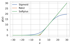
Figure 2: Link functions $\phi$ of the Hawkes model considered in Simulation 1, namely the sigmoid (blue), ReLU (red), and softplus (green) functions.

In this simulation, we consider univariate Hawkes processes ($K=1$) with link function $\phi=\phi_{1}$ of the form

$$\phi(x)=\theta+\Lambda\psi(\alpha(x-\eta)),$$ (29)

where $\xi=(\theta,\Lambda,\alpha,\eta)$ and $\psi:\varmathbb R\to\varmathbb R^{+}$ are known and chosen as:

• Sigmoid: $\psi(x)=(1+e^{-x})^{-1}$ and $\xi=(0.0,20.0,0.2,10.0)$;

• ReLU: $\psi(x)=\max(x,0)$ and $\xi=(0.001,1.0,1.0,0.0)$;

• Softplus: $\psi(x)=\log(1+e^{x})$ and $\xi=(0.0,40.0,0.1,20.0)$.

Note that the corresponding link functions $\phi$ have similar shapes on a range of values between -20 and 20 (see Figure 2). In all models, we consider a Hawkes process with $h_{0}=h_{11}^{0}\in\mathcal{H}_{histo}^{D_{0}}$ with $D_{0}=2$, and three scenarios, called Excitation only, Mixed effect, and Inhibition only, where $h_{0}$ is respectively non-negative, signed, and non-positive (see Figure 3 for instance). In each of the nine settings, we set $T=500$ and in Table 1, we report the corresponding number of events and excursions observed in each scenario and model. Note that, as we may expect, more events and less excursions are observed in the data generated in Excitation only scenario than in the Mixed effect and Inhibition only scenarios.

Here, we assume that $D_{0}$ is known and we consider a normal prior on $\mathcal{H}_{histo}^{D_{0}}$ such that $w_{11}\sim\mathcal{N}(0,\sigma^{2}I),$ and for $\nu_{1}$, $\nu_{1}\sim\mathcal{N}(0,\sigma^{2}),$ with $\sigma=5.0$. To compute the (true) posterior distribution, we run a Metropolis-Hasting (MH) sampler implemented via the Python package PyMC4 with 4 chains, 40 000 iterations, and a burn-in time of 4000 iterations. We also use the Gaussian quadrature method (Golub and Welsch, 1969) for evaluating the log-likelihood function, except in the ReLU model and Excitation only scenario, where the integral term is computed exactly. We note that we also tested a Hamiltonian Monte-Carlo sampler in this simulation, and obtained similar posterior distributions, but within a much larger computational time, therefore these results are excluded from this experiment.

The posterior distribution on $f=(\nu_{1},h_{11})$ in the ReLU model and our three scenarios are plotted in Figure 3. For conciseness purpose in this section, our results for the sigmoid and softplus models are reported in Appendix F.1. We note that in almost all settings, the ground-truth parameter $f_{0}$ is included in the 95% credible sets of the posterior distribution. Nonetheless, the posterior mean is sometimes biased, possibly due to the numerical integration errors in the log-likelihood computation. Moreover, we conjecture that the estimation quality depends on the number of events and the number of excursions, which could explain the differences between the Excitation only, Mixed effect, and Inhibition only scenarios. In particular, the credible sets seem consistently smaller for the second scenario, which realisations have more excursions than the other ones.

This simulation therefore shows that the posterior distribution in commonly used nonlinear univariate Hawkes models behaves well and can be sampled from using a simple MH sampler. Nonetheless, we note that the MH iterations are computationally expensive, which prevents from scaling this algorithm to large dimensions. Therefore, we will only use the MH sampler to compute the posterior distribution in the low-dimensional settings, i.e., Simulations 2 and 3, with respectively $K=1$ and $K=2$.

Scenario		Sigmoid	ReLU	Softplus
Excitation only	# events	5250	5352	4953
	# excursions	1558	1436	1373
Mixed effect	# events	3876	3684	3418
	# excursions	1775	1795	1650
Inhibition only	# events	3047	2724	2596
	# excursions	1817	1693	1588

Table 1: Number of events and excursions in the simulated data of Simulation 1 with $T=500$. We refer to Remark 11 and Lemma 12 in Appendix D.1 for the definition of an excursion in Hawkes processes.

ReLU Excitation only Mixed effect Inhibition only
Background
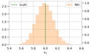
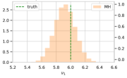
Interaction

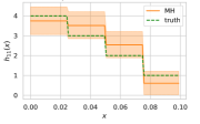
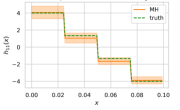
Figure 3: Posterior distribution on $f=(\nu_{1},h_{11})$ obtained with the Metropolis-Hastings sampler (MH), in the univariate ReLU models of Simulation 1. The three columns correspond to the Excitation only (left), Mixed effect (center), and Inhibition only (right) scenarios. On the first row, we plot the marginal posterior distribution on the background rate $\nu_{1}$, and on the second row, the posterior mean (solid orange line) and 95% credible sets (orange areas) on the interaction function $h_{11}$, here piecewise-constant with dimensionality $2^{D_{0}}=4$. The true parameter $f_{0}=(\nu_{1}^{0},h_{11}^{0})$ is plotted in dotted green line.

5.2 Simulation 2: Parametric variational posterior and posterior distribution in the univariate sigmoid model.

In this simulation, we consider the same univariate scenarios as Simulation 1, but only for the sigmoid Hawkes model and compare the variational and true posterior distributions. Here, the dimensionality $D_{0}$ of the true function $h_{0}$ is assumed to be known, therefore, the samplers are non-adaptive. Specifically, we compare the performance of the previous MH sampler, the Gibbs sampler (introduced in Remark 4 and described in Algorithm 4 in Appendix  C.3), and our mean-field variational algorithm in a fixed model (Algorithm 1) - here, we fix the dimensionality of $h_{11}$ to $J=2^{D_{0}}=4$. We run 4 chains for 40 000 iterations for the MH sampler, 3000 iterations of the Gibbs sampler, and use our early-stopping procedure for the mean-field variational algorithm.

In Figure 4, we can compare the variational posterior on $f=(\nu_{1},h_{11})$ to the posterior distributions, computed either with the Gibbs or MH samplers, in the three estimation scenarios. We note that variational posterior mean is always close to the posterior mean, in particular when computed with the Gibbs sampler. Nonetheless, its credible sets are generally smaller, which is a common empirical observation of mean-field variational approximations.

Besides, the variational posterior seems to be similarly biased as the posterior distribution, as can be seen for the background rate $\nu_{1}$ in the Inhibition scenario. One could therefore test if this bias decreases with more data observations, i.e., larger $T$; however, the Gibbs sampler has a large computational time (between 3 and 5 hours), which is about 6 (resp. 40) times longer than the MH sampler (resp. our mean-field algorithm), due to the expensive latent variable sampling scheme (see Table 2). Finally, we also compare the estimated intensity function using the (variational) posterior means, on a sub-window of the observations in Figure 5. The latter plot shows that all three methods provide fairly equivalent estimates on the nonlinear intensity function.

From this simulation, we conclude that, in the univariate and parametric sigmoid Hawkes model, the mean-field variational algorithm in a fixed model provides a good approximation of the posterior distribution. Moreover, we note that although the Gibbs sampler is slightly better than MH, it is much slower than the latter and therefore cannot be applied to multivariate Hawkes processes in practice. Therefore, in the bivariate simulation in the next section, we only compare to the posterior distribution computed with the MH sampler, which can still be computed within reasonable time for $K=2$ .

Scenario	MH	Gibbs	MF-VI
Excitation only	2169	16 092	416
Mixed effect	2181	13 097	338
Inhibition only	2222	9 318	400

Table 2: Computational times (in seconds) of the Gibbs sampler (Algorithm 4), our mean-field variational (MF-VI) algorithm (Algorithm 1), and the Metropolis-Hastings (MH) sampler in each parametric univariate scenario of Simulation 2 with $T=500$. We note that the Gibbs sampler is much slower than the MH sampler, which is also slower than the mean-field variational algorithm.

Sigmoid Excitation only Mixed effect Inhibition only
Background
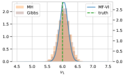
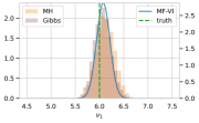
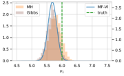
Interaction

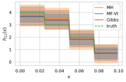
Figure 4: Posterior and variational posterior distributions on $f=(\nu_{1},h_{11})$ in the univariate sigmoid model of Simulation 2, evaluated by the MH sampler, the mean-field variational (MF-VI) algorithm in a fixed model (Algorithm 1) and the Gibbs sampler (Algorithm 4). The three columns correspond to the Excitation only (left), Mixed effect (center), and Inhibition only (right) scenarios. The true parameter $f_{0}$ is plotted in dotted green line. The first row contains the marginal distributions (VB, MH and Gibbs) on the background rate $\nu_{1}$, and the second row represents the posterior means (solid lines) and 95% credible sets (colored areas) on the (self) interaction function $h_{11}$. We note that the variational posterior is close to the Gibbs posterior distribution, nonetheless, has smaller credible bands.

(a) Excitation only

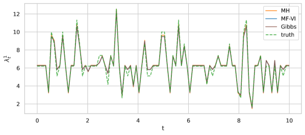
(b) Mixed effect

(c) Inhibition only

Figure 5: Intensity function on a sub-window of the observation window estimated via the variational posterior mean (blue) or via the posterior mean, computed with the MH sampler (orange) or the Gibbs sampler (purple), in each scenario of Simulation 2. The true intensity $\lambda_{t}^{1}(f_{0})$ is plotted in dotted green line. We note that all estimates are close in this simulation.

5.3 Simulation 3: Fully-adaptive variational method in the univariate and bivariate sigmoid models.

# dimensions	Scenario	T	FA-MF-VI	MH
$K=1$	Excitation	2000	32	417
	Inhibition	3000	33	445
$K=2$	Excitation	2000	189	2605
	Inhibition	3000	197	2791

Table 3: Computing times (in seconds) of our fully-adaptive mean-field variational method (FA-MF-VI) (Algorithm 2) and the Metropolis-Hastings (MH) sampler in the univariate and bivariate sigmoid models and the scenarios of Simulation 3.

In this simulation, we test our fully-adaptive variational inference algorithm (Algorithm 2), in the one-dimensional ($K=1$) and two-dimensional ($K=2$) sigmoid models, and in two estimation settings:

1. Well-specified: $h_{0}\in\mathcal{H}_{hist}^{D_{0}}$ (with $D_{0}=2$);

2. Mis-specified: $h_{0}\notin\mathcal{H}_{hist}^{D_{0}}$, and $h_{lk}^{0}$ is a continuous function, for all $(l,k)\in[K^{2}]$.

Note that in the well-specified case, $m_{0}:=(\delta_{0},2^{D_{0}})$ is unknown for the variational method, nonetheless, we also compute the posterior distribution with the non-adaptive MH sampler using the true $m_{0}$. In the bivariate model, we choose a true graph parameter $\delta_{0}$ with one zero entry (see Figure 8a). We also consider an Excitation scenario where all the true interaction functions $(h_{lk}^{0})_{l,k}$ are non-negative and with $T=2000$, and an Inhibition scenario where the self-interaction functions $(h_{kk}^{0})_{k=1,2}$ are non-positive with $T=3000$. The latter setting aims at imitating the so-called self-inhibition phenomenon in neuronal spiking data, due to the refractory period of neurons (Bonnet et al., 2021). In our adaptive variational algorithm, we set a maximum histogram depth $D_{1}=5$ for $K=1$, and $D_{1}=4$ for $K=2$, so that the number of models per dimension is respectively 7 and 76.

In the well-specified setting, we first analyse the ability of Algorithm 2 to recover the true connectivity graph and dimensionality of $h_{0}$. In Figure 6, we plot the model marginal probabilities $(\hat{\gamma}_{m})_{m}$ in our adaptive variational posterior and in the univariate setting. In the Excitation scenario, the largest marginal probability $\hat{\gamma}_{\hat{s}}$ is on the true model, i.e., $\hat{m}=m_{0}=(\delta_{0}=1,2^{D_{0}}=2)$, and all the other marginal probabilities are negligible. Therefore, in this case, the model-averaging VB posterior (13) is essentially equivalent to the model-selection VB posterior (12). In the Inhibition scenario, the dimensionality $\hat{D}$ is not well inferred in the model selection variational posterior (maximising the ELBO), which is over-regularizing in this case, since $\hat{m}=(\hat{\delta}=\delta_{0}=1,\hat{D}=1)$. However, as seen in Figure 6, the ELBO for $D=1$ and for $D=2=D_{0}$ are very close, therefore, the model-averaging variational posterior better captures the model since itis essentially a mixture of two components, one corresponding to $\hat{D}=1$, and the second one corresponding to the true model $D_{0}+2$.

Nonetheless, comparing the estimated nonlinear intensity based on the model-selection variational posterior mean and the posterior mean in Figure 26 in Appendix F, we note that the model selection variational estimate is very close to the true intensity and the non-adaptive MH estimate, despite the error of dimensionality in the Inhibition scenario.

We then compare the model selection adaptive variational posterior distribution on the parameter with the true posterior distribution computed with the non-adaptive MH sampler in Figure 7. We note that in the Excitation scenario, the variational posterior mean is very close to the posterior mean, however, its 95% credible bands are significantly smaller. Note also that, in the Inhibition scenario, in spite of the wrongly selected histogram depth, the estimated interaction function is still not too far from the truth.

In the mis-specified setting, all the marginal probabilities are negligible but one, in both the Excitation and Inhibition scenarios (see Figure 6), although there is no true $m_{0}$ in this case. In Figure 28 in Appendix F, we note that the model selection adaptive variational posterior mean approximates quite well the true parameter. Moreover, its 95% credible bands often cover the truth but are once again slightly too narrow.

The previous observations in the well-specified and mis-specified settings can also be made in the two-dimensional setting. The true connectivity graph and the marginal probabilities in the adaptive variational posterior are plotted in Figure 8. We note that in the well-specified case, $\hat{m}=m_{0}$ in both scenarios. Moreover, the parameter and the nonlinear intensity are well estimated, as can be seen in Figure 10 and in Figures 27, 29 in Appendix F. Note however that, in the mis-specified setting, the under-coverage phenomenon of the credible regions also occurs (see Figure 9).

Finally, we note that our fully-adaptive variational algorithm is more than 10 times faster to compute than the non-adaptive MH sampler, as can be seen from the computing times reported in Table 3. This simulation study therefore shows that our fully-adaptive variational algorithm enjoys several advantages in Bayesian estimation for Hawkes processes: it can infer the dimensionality of the interaction functions $D$, the dependence structure through the graph parameter $\delta$, provides a good approximation of the posterior mean, and is computationally efficient.

$K=1$ Excitation Inhibition
Well-specified
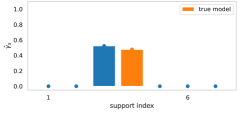
Mis-specified

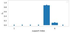
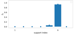
Figure 6: Model marginal probabilities $(\hat{\gamma}_{m})_{m}$ in the adaptive mean-field variational posterior, in the well-specified and mis-specified settings of Simulation 3 with $K=1$. The left and right panels correspond to the Excitation (resp. Inhibition) setting. The elements in $\mathcal{S}_{1}$ are indexed from 1 to 7, and correspond respectively to $m=(\delta=0,2^{D}=1)$, and $m=(\delta=1,2^{D})$ with $D=0,\dots,5$.

$K=1$ Well-specified-Exc Well-specified-Inh Mis-specified-Exc
Background
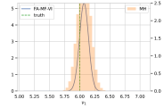
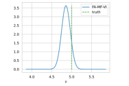
Interaction

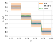
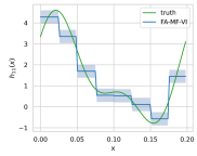
Figure 7: Posterior and model-selection variational posterior distributions on $f=(\nu_{1},h_{11})$ in the univariate sigmoid model and settings of Simulation 3, evaluated by the MH sampler and the fully-adaptive mean-field variational (FA-MF-VI) algorithm (Algorithm 2). The three columns correspond respectively to the two well-specified settings, i.e., the Excitation (Well-specified-Exc) and Inhibition (Well-specified-Exc) scenarios, and one mis-specified setting (Mis-specified-Exc). The first row contains the marginal distribution on the background rate $\nu_{1}$, and the second row represents the (variational) posterior mean (solid line) and 95% credible sets (colored areas) on the (self) interaction function $h_{11}$. The true parameter $f_{0}$ is plotted in dotted green line.

(a) Excitation

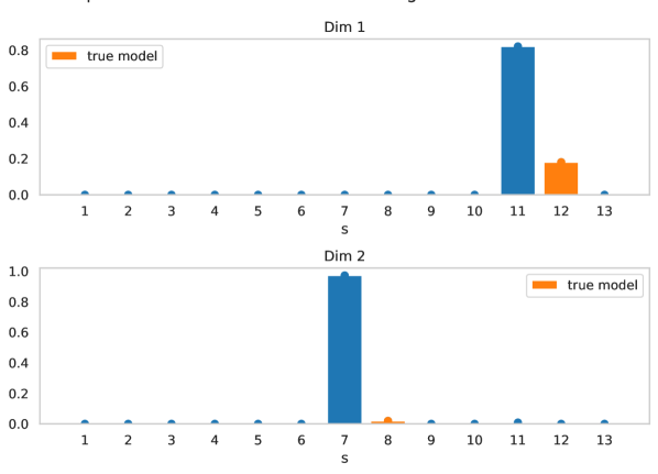
(b) Inhibition

Figure 8: Marginal probabilities on the graph and dimensionality parameter $s_{k}=(\delta_{\cdot,k},D_{k})$ at each dimension, i.e., $(\hat{\gamma}_{s_{k}}^{k})_{s_{k}\in\mathcal{S}_{2}}$ in the fully-adaptive averaged mean-field variational posterior, in the well-specified setting of Simulation 3 with $K=2$. The Excitation scenario (8(a)) corresponds to $h_{0}\geqslant 0$, while in the Inhibition scenario (8(b)) , $h_{11}^{0},h_{22}^{0}\leqslant 0$. The elements in $\mathcal{S}_{2}$ are indexed from 1 to 13 and the true model in this set is indicated in orange.

$K=2$ Well-specified Mis-specified
                  Background
                                    Interaction functions

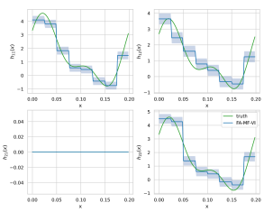
Figure 9: Model-selection variational posterior distributions on $f=(\nu,h)$ in the bivariate sigmoid model, and well-specified and mis-specified settings, and Excitation scenario of Simulation 3, computed with the fully-adaptive mean-field variational (FA-MF-VI) algorithm (Algorithm 2). The first row correspond two columns correspond to the Excitation (left) and Inhibition (right) settings. The first row contains the marginal distribution on the background rates $(\nu_{1},\nu_{2})$, and the second and third rows represent the (variational) posterior mean (solid line) and 95% credible sets (colored areas) on the four interaction function $h_{11},h_{12},h_{21},h_{22}$. The true parameter $f_{0}$ is plotted in dotted green line.

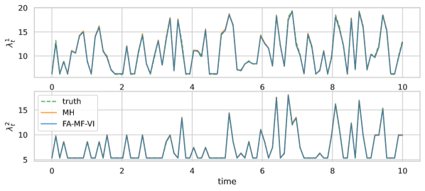
(a) Excitation scenario

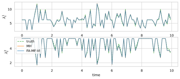
(b) Self-inhibition scenario

Figure 10: Estimated intensity function based on the (variational) posterior mean, in the well-specified and bivariate setting of Simulation 3 on $[0,10]$, using the fully-adaptive mean-field variational (FA-MF-VI) algorithm (Algorithm 2). The true intensity $\lambda_{t}(f_{0})$ is plotted in dotted green line.

5.4 Simulation 4: Two-step variational posterior in high-dimensional sigmoid models.

In this section, we test the performance of our two-step variational procedure (Algorithm 3), first, in sparse settings of the true parameter $h_{0}$, then, in relatively denser regimes.

5.4.1 Sparse settings

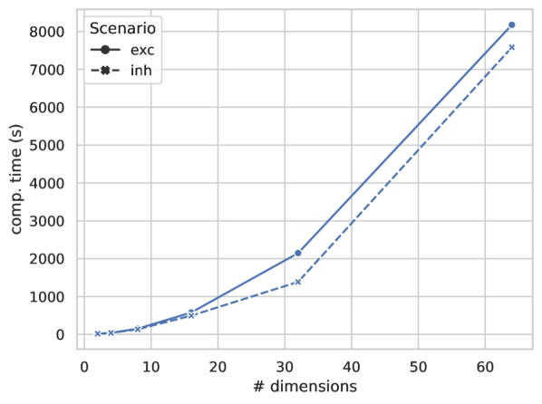
Figure 11: Computational times of our two-step mean-field variational algorithm (Algorithm 3) in the Excitation (exc) and Inhibition (inh) scenarios and well-specified setting of Simulation 4, for $K=2,4,8,16,32,64$.

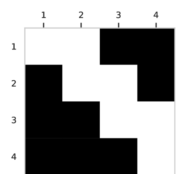
(b) $K=4$

(c) $K=8$

(d) $K=10$

(e) $K=16$

(f) $K=32$

Figure 12: True graph parameter $\delta_{0}$ (black=0, white=1) in the sparse multivariate settings of Simulations 4 with the number of dimensions $K=2,4,8,16,32,64$.

In this experiment, we consider sparse multivariate sigmoid models with $K\in\{2,4,8,16,32,64\}$ dimensions. We note that to the best of our knowledge, the only Bayesian method that has currently been tested in high-dimensional Hawkes processes is the semi-parametric version of Zhou et al. (2022) where the interaction functions are also decomposed over a dictionary of functions, but the choice of the number of functions is not driven by a model selection procedure and the graph of interaction is not inferred. Here, we construct a well-specified setting with $h_{0}\in\mathcal{H}_{hist}^{D_{0}}$ and $D_{0}=1$, and an Excitation scenario and an Inhibition scenario, similar to Simulation 3, and a sparse connectivity graph parameter $\delta_{0}$ with $\sum_{l,k}\delta_{lk}^{0}=2K-1$, as shown in Figure 12. In Table 4, we report our chosen value of $T$ in each setting and the corresponding number of events, excursions, and local excursions. In Table 6, we report the performance of our method, in terms of the $L_{1}$-risk of the model-selection variational posterior defined as

$$r_{L_{1}}(\hat{Q}):=\varmathbb{E}_{\hat{Q}}[\left\lVert\nu-\nu_{0}\right\rVert_{\ell_{1}}]+\sum_{l,k}\varmathbb{E}_{\hat{Q}}\left[\left\lVert h_{lk}-h_{lk}^{0}\right\rVert_{1}\right].$$ (30)

We note that in general, the number of terms in the risk grows with $K$ and the number of non-null interaction functions in $h$ and $h_{0}$ - which thus can be of order $O(K^{2})$ in a dense setting.

We first note that for our prior distribution and for the augmented variational posterior distribution $\hat{Q}$ in a fixed model $m=(\delta,J=(J_{k}))$, we have that

$$\varmathbb{E}_{\hat{Q}_{1}}[\left\lVert h_{lk}\right\rVert_{1}] =\sum_{j=1}^{J_{k}}\sqrt{\frac{2}{\pi}[\Sigma_{lk}^{J_{k}}]_{jj}}\exp\left\{-\frac{[\tilde{\mu}_{lk}^{J_{k}}]_{j}^{2}}{[\Sigma_{lk}^{D_{k}}]_{jj}}\right\}-[\tilde{\mu}_{lk}^{J_{k}}]_{j}\left[1-2\Phi\left(-\frac{[\tilde{\mu}_{lk}^{J_{k}}]_{j}}{\sqrt{[\Sigma_{lk}^{J_{k,C}}]_{jj}}}\right)\right].$$

We evaluate the accuracy of our algorithm when estimating the graph of interaction and the size $D_{k}$ at each dimension $k$, defined as

$$Acc_{graph}(\hat{\delta})=\frac{1}{K^{2}}\sum_{l,k}\mathds{1}_{\delta_{lk}^{0}=\hat{\delta}_{lk}}, Acc_{dim}(\hat{D})=\frac{1}{K}\sum_{k}\mathds{1}_{D_{k}^{0}=\hat{D}_{k}},$$

where $\hat{\delta}=(\hat{\delta}_{lk})_{l,k}$ and $\hat{D}=(\hat{D}_{k})_{k}$ are respectively the estimated graph and the inferred dimensionality of $(h_{.k})_{k}$ in Algorithm 3.

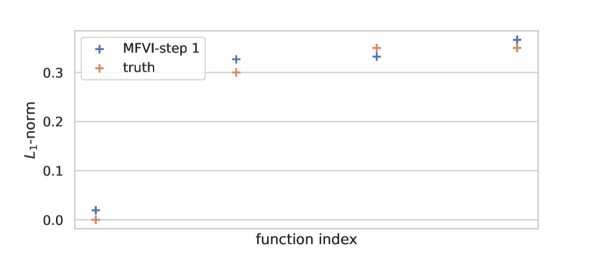
(a) $K=2$

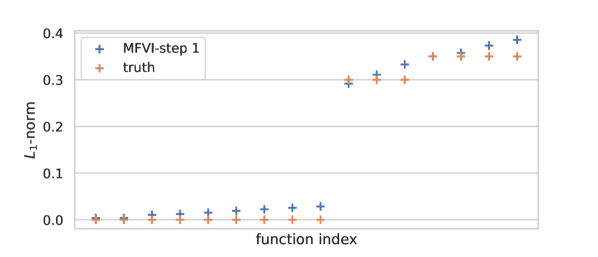
(b) $K=4$

(c) $K=8$

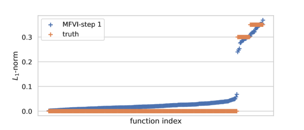
(d) $K=16$

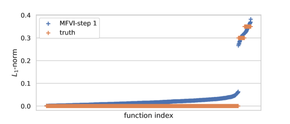
(e) $K=32$

(f) $K=64$

Figure 15: Estimated $L_{1}$-norms using the model-selection variational posterior obtained after the first step of Algorithm 3, plotted in increasing order, in the Excitation scenario of Simulation 4, for the models with $K=2,4,8,16,32,64$. In these settings, our threshold $\eta_{0}=0.15$ is included in the gap between the estimated norms close to 0 and far from 0, therefore, our gap heuristics allows to recover the true graph parameter (see Section 3.2.2).

Firstly, we note that, in almost all settings, the accuracy of our algorithm is equal or is very close to 1, therefore, it is able to recover almost perfectly the true graph $\delta_{0}$ and the dimensionality $D_{0}$ (the estimated graphs in the Excitation and Inhibition scenarios are plotted in Figures 30 and 31 in Appendix). In fact, our gap heuristics for choosing the threshold $\eta_{0}$ (see Section 3.2.2) allows to estimate the graph after the first step of Algorithm 3. In Figure 15 (and Figure 33 in Appendix in the Inhibition scenario), we note that the $L_{1}$-norms of the interaction functions are well estimated in the first step, leading to a gap between the norms close and far from 0. This gap includes the range $[0.1,0.2]$ for all $K$’s, therefore, here, we choose $\eta_{0}=0.15$, which allows to discriminate between the true signals and the noise and to recover the true graph parameter.

Excitation $K=2$ $K=4$ $K=16$ $K=64$
Ground-
truth
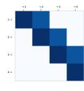
Error

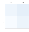
Figure 14: Heatmaps of the $L_{1}$-norms of the true parameter $h_{0}$, i.e., the entries of the matrix $S_{0}=(S^{0}_{lk})_{l,k}=(\left\lVert h_{lk}^{0}\right\rVert_{1})_{l,k}$ (left column) and the $L_{1}$-risk of the model-selection variational posterior obtained with Algorithm 3, i.e., $(\varmathbb{E}^{\hat{Q}_{MV}}[\left\lVert h_{lk}^{0}-h_{lk}\right\rVert_{1}])_{l,k}$ (right column), in the Excitation scenario of Simulation 4. The rows correspond to $K=2,4,8,16,32,64$.

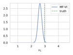
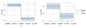
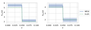
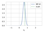
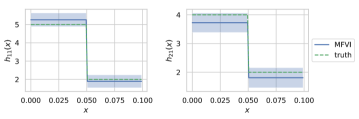
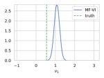
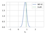
Figure 18: Model-selection variational posterior distributions on $\nu_{1}$ (left column) and interaction functions $h_{11}$ and $h_{21}$ (second and third columns) in the Excitation scenario and multivariate sigmoid models of Simulation 4, computed with our two-step mean-field variational (MF-VI) algorithm (Algorithm 3). The different rows correspond to different multivariate settings $K=2,4,8,16,32,64$.

Secondly, from Table 6, we note that the risk seems to grow linearly with $K$, which indicates that the estimation does not deteriorate with larger $K$. In Figure 14 (and Figure 32 in Appendix, we plot the risk on the $L_{1}$-norms using the model-selection variational posterior, i.e., $(\varmathbb{E}_{\hat{Q}_{MV}}\left[\left\lVert h_{lk}-h_{lk}^{0}\right\rVert_{1}\right])_{l,k}$, in the form of a heatmap compared to the true norms, and note that for all $K$’s, these errors are relatively small. Moreover, our variational algorithm estimates well the parameter, as can be visually checked in Figure 18, where we plot the model-selection variational posterior distribution on a subset of the parameter for each value of $K$, in the Excitation scenario (see Figure 34 in Appendix for our results in the Inhibition scenario). Besides, the computing times of our algorithm seem to scale well with $K$ and the number of events in these sparse settings, as can be seen from Table 4 and Figure 11. For $K=64$, our algorithm runs in less than 2.5 hours, in spite of the large number of events (about 133 000). We also note that these experiments have been run using only two processing units.

5.4.2 Testing different graphs and sparsity levels.

In this experiment, we evaluate Algorithm 3 on different settings of the graph parameter $\delta_{0}$, namely a sparse, a random, and a dense settings, illustrate in Figure 13. The sparse setting is similar to the previous section, while the random setting corresponds to a slightly less sparse regime where additional edges are present in $\delta_{0}$. Note that these three settings have different numbers of edges in $\delta_{0}$, therefore, different numbers of non-null interaction functions to estimate. From Table 5, we also note that there are more events and less global excursions in the dense setting that in the two other ones, in particular, in the Excitation scenario where this number drops to 2.

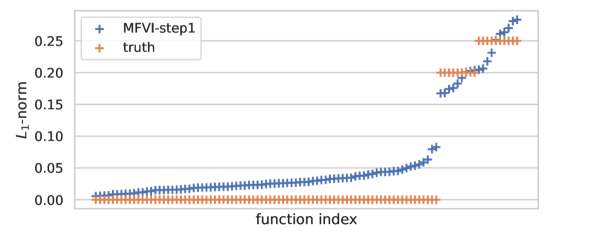
(b) Inhibition - sparse

(c) Excitation - random

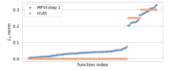
(d) Inhibition - random

(e) Excitation - dense

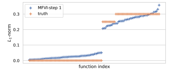
(f) Inhibition - dense

Figure 16: Estimated $L_{1}$-norms using the model-selection variational posterior obtained after the first step of Algorithm 3, plotted in increasing order, in the different graph settings (sparse, random, and dense $\delta_{0}$, see Figure 13) and scenarios of Simulation 4 with $K=10$. We note that in the dense graph setting, although the norms are not very well estimated after the first step, the gap heuristics still allows to recover the true graph parameter.

Our numerical results in Table 7 show that in the dense setting, the graph accuracy of our estimator is slightly worse, and the risk of the variational posterior is much higher than in the other settings. We conjecture that this loss of performance is related to the smaller number of global excursions, which leads to a more difficult estimation problem. We can also see from Figure 16 that in this particular setting, the estimation of the norms of the interaction functions is deteriorated, and the gap that allows to discriminate between the null and non-null functions is not present anymore. Nonetheless, in the Inhibition scenario, for which the number of global excursions is not too small, this phenomenon does not happen and the estimation is almost equivalent in all graph settings.

To further explore the applicability of our thresholding approach in the dense setting, we test the following three-step approach in the Excitation scenario, with $K=10$ and a dense graph $\delta_{0}$:

• The first step is similar to the one of our two-step procedure, i.e., we estimate an adaptive variational posterior distribution within models that contain the complete graph $\delta_{C}$.

  Then, if there is no significant gap in the variational posterior mean estimates of the $L_{1}$-norms, we look for a (conservative) threshold $\eta_{1}$ corresponding to the first “slope change”, and estimate a (dense) graph $\hat{\delta}$.

• In a second step, we compute the adaptive variational posterior distribution within models that contain $\hat{\delta}$ and re-estimate the $L_{1}$-norms of the functions.

  If we now see a significant gap in the norms estimates, we choose a second threshold within that gap; otherwise, we look again for a slope change and pick a conservative threshold $\eta_{2}$ to compute a second graph estimate $\hat{\delta}_{2}$.

• In the third and last step, we repeat the second step with now our second graph estimate, $\hat{\delta}_{2}$.

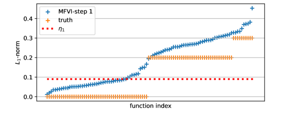
(b) Step 1

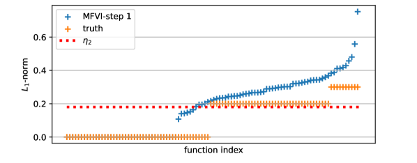
(c) Step 2

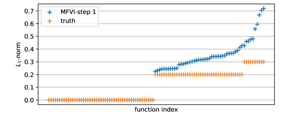
(d) Step 3

Figure 17: True graph $\delta_{0}$ and estimated $L_{1}$-norms using the model selection adaptive variational posterior obtained after each step of our three-step procedure, proposed for the dense graph setting of Simulation 4. In Step 1 and Step 2, we plot the data-driven thresholds $\eta_{1}$ and $\eta_{2}$, chosen with a “slope change” heuristics.

In Figure 17, we plot our estimates of the norms after each step of the previous procedure. In this case, we have chosen visually the threshold $\eta_{1}=0.09$ and $\eta_{2}=0.18$ after respectively the first and second step, using the slope change heuristics. We note that the previous method indeed provides a conservative graph estimate in the first step, but in the second step, allows to refine our estimate of the graph and approach the true graph. Besides, we note that the large norms are inflated along the three steps of our procedure. Therefore, our method performs better in sparse settings where a significant gap allows to correctly infer the true graph $\delta_{0}$.

In conclusion, our simulations in low and high-dimensional settings, with different levels of sparsity in the graph, show that our two-step procedure is able to correctly select the graph parameter and dimensionality of the process in sparse settings, and hence allows to scale up variational Bayes approaches to larger number of dimensions. Nonetheless, from the moderately high-dimensional settings, the estimation of the parameter $f$ becomes sensitive to the difficulty of the problem. In particular, the performance is sensitive to the graph sparsity, tuning the number of non-null functions to estimate, and, as we conjecture, the number of global excursions in the data. Finally, we note that heuristic approaches for the choice of the threshold - needed to estimate the graph parameter - need to further explored in noisier and denser settings.

K	Scenario	T	# events	# excursions	# local excursions	computing time (s)
2	Excitation	500	5680	2416	1830	19
	Inhibition	700	4800	2416	1830	18
4	Excitation	500	11338	2378	1878	41
	Inhibition	700	9895	2378	1878	39
8	Excitation	500	22514	1207	1857	151
	Inhibition	700	19746	1207	1857	134
16	Excitation	500	51246	200	1784	577
	Inhibition	700	37166	200	1784	494
32	Excitation	500	96803	4	1824	2147
	Inhibition	700	76106	4	1824	1386
64	Excitation	200	117862	0	1481	8176
	Inhibition	300	133200	0	1481	7583

Table 4: Number of observed events, excursions, and computing times of Algorithm 3 in the multivariate settings of Simulation 4.

Scenario	Graph	# Edges	# Events	# Excursions	# Local excursions
Excitation	Sparse	$2K-1$	24638	431	1212
	Random	$3K-1$	27475	398	1262
	Dense	$5K-6$	90788	2	1432
Inhibition	Sparse	$2K-1$	22683	911	1778
	Random	$3K-1$	24031	884	1834
	Dense	$5K-6$	35291	547	2170

Table 5: Number of edges, observed events, and excursions in the different graph settings of Simulation 4 ($K=10$).

# dimensions	Scenario	Graph accuracy	Dimension accuracy	Risk
2	Excitation	1.00	1.00	0.79
	Inhibition	1.00	1.00	0.35
4	Excitation	1.00	1.00	1.01
	Inhibition	1.00	1.00	0.92
8	Excitation	1.00	1.00	2.10
	Inhibition	1.00	1.00	2.12
16	Excitation	1.00	1.00	5.77
	Inhibition	1.00	1.00	4.48
32	Excitation	1.00	0.97	10.57
	Inhibition	1.00	1.00	8.53
64	Excitation	1.00	1.00	23.74
	Inhibition	1.00	1.00	18.43

Table 6: Performance of Algorithm 3 in the multivariate settings of Simulation 4. We report the accuracy of our graph estimate $\hat{\delta}$ and the selected dimensionality of the interaction functions in the model-selection variational posterior, and the risk on the whole parameter $f$ defined in (30).

Scenario	Graph	Graph accuracy	Dimension accuracy	Risk
Excitation	Sparse	1.00	1.00	2.91
	Random	1.00	1.00	4.00
	Dense	0.5	1.00	17.67
Inhibition	Sparse	1.00	1.00	2.62
	Random	0.99	1.00	3.44
	Dense	1.00	1.00	2.67

Table 7: Performance of Algorithm 3 in the different graph settings of Simulation 4 ($K=10$). We note in that the dense graph setting, there are more parameters to estimate, and therefore non-null terms in the risk metric.

(a) $K=2$

(a) sparse

(b) random

(c) dense

Figure 13: True graph parameter $\delta_{0}$ (black=0, white=1) in the sparse, random, and dense settings of Simulations 4 with $K=10$ dimensions.

(a) Excitation - sparse

(a) True graph $\delta_{0}$

Excitation Background $\nu_{1}$ Interaction functions $h_{11}$ and $h_{21}$

5.5 Simulation 5: Convergence of the two-step variational posterior for varying data set sizes.

In this experiment, we study the variations of performances of Algorithm 3 with increasing lengths of the observation window, i.e., increasing number of data points. We consider multidimensional data sets with $K=10$, $T\in\{50,200,400,800\}$, the same connectivity graph as in Simulation 4, and an Excitation and an Inhibition scenarios. The number of events and excursions in each data sets are reported in Table 10 in Appendix F.4.

We estimate the parameters using the model-selection variational posterior in Algorithm 3 for each data set. From Table 8, we note that our graph estimator converges quickly to the true graph and the risk also decreases with the number of observations. We can also see from Figure 19 that the estimation of the $L_{1}$-norms after the first step of the algorithm improves for larger $T$, leading to a bigger gap between the small and large norms. Finally, in Figure 20 (and Figure 35 in Appendix), we plot the model-selection variational posterior and note that its mean gets closer to the ground-truth parameter and its credible set shrinks for larger $T$.

Scenario	T	Graph accuracy	Dimension accuracy	Risk
Excitation	50	1.00	0.40	7.06
	200	1.00	1.00	5.07
	400	1.00	1.00	5.06
	800	1.00	1.00	4.01
Inhibition	50	0.98	0.40	8.61
	200	1.00	1.00	4.30
	400	1.00	1.00	3.96
	800	1.00	1.00	2.91

Table 8: Performance of Algorithm 3 for the different data set sizes $T\in\{50,200,400,800\}$ in the scenarios of Simulation 5 with $K=10$. We note the graph estimator quickly converges to the true graph $\delta_{0}$.

(a) Excitation scenario

(b) Inhibition scenario

Figure 19: Estimated $L_{1}$-norms after the first step of Algorithm 3, for different observation lengths $T$, in the Excitation and Inhibition scenarios of Simulation 5 with $K=10$. We note that the norms are better estimated, after the first step of our algorithm, for larger $T$, leading to a larger gap between the small and large estimated norms, in both scenarios.

(a) Excitation scenario

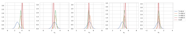
(b) Inhibition scenario

Figure 20: Model-selection adaptive variational posterior on a subset of background rates, $(\nu_{1},\dots,\nu_{5})$, for different observation lengths $T\in\{50,200,400,800\}$, in the Excitation and Inhibition scenarios in Simulation 5 with $K=10$. The variational posterior behaves as expected in this simulation: as $T$ increases, its mean gets closer to the ground-truth parameter and its variance decreases.

5.6 Simulation 6: robustness to mis-specification of the link function and the memory parameter

In this experiment, we first test the robustness of our variational method based on the sigmoid model parametrised by (29) with $\xi=(0.0,20.0,0.2,10.0)$ to mis-specification of the nonlinear link functions $(\phi_{k})_{k}$. Specifically, we set $K=10$ and construct synthetic mis-specified data by simulating a Hawkes process where for each $k$, the link $\phi_{k}$ is chosen as:

• ReLU: $\phi_{k}(x)=(x)_{+}$;

• Softplus: link $\phi_{k}(x)=\log(1+e^{x})$;

• Mis-specified sigmoid, with unknown $\theta_{k}\overset{i.i.d.}{\sim}U([15,25])$.

We also consider Excitation and Inhibition scenarios. Here, $T=300$ in all settings.

In Figure 21, we plot the estimated $L_{1}$-norms after the first step of Algorithm 3 and note that there is still a gap in all settings and scenarios, although the norms are not well estimated in the case of the ReLU and softplus nonlinearities. The gaps allow to estimate well the connectivity graph parameter, but the other parameters cannot be well estimated for these two links, as can be seen from the risks in Table 9. Nonetheless, the sign of the interaction functions is well recovered in all settings.

Then, we test the robustness of our variational method to mis-specification of the memory parameter $A$, assumed to be known in our framework. We recall that $A$ corresponds to the upper bound of the support of the interaction functions. For this experiment, we generate data from the sigmoid Hawkes process with $K=10$ and with ground-truth parameter $A_{0}=0.1$, in two sets of parameters corresponding to an Excitation and an Inhibition scenarios. Here, we set $T=500$ and apply our variational method (Algorithm 3) with $A\in\{0.5,0.1,0.2,0.4\}$.

In Figure 22(b), we plot the estimated $L_{1}$-norms of the interaction functions, after the first step of Algorithm 3, when using the different values of $A$. We note that when $A$ is smaller than $A_{0}$, the norms of the non-null functions are underestimated, while if $A$ is larger than $A_{0}$, the norms are slightly overestimated. We note that, in all settings, the graph can be well estimated with the gap heuristics (see Figure 38 in Appendix). The model-selection variational posterior on a subset of the interaction functions is plotted in Figure 23. We note that for $A=0.05=A_{0}/2$, only the first part of the functions can be estimated, while for $A>A_{0}$, the mean estimate is close to 0 on the upper part of the support. Nonetheless, in the latter case, the dimensionality of the true functions is not well-recovered.

In conclusion, this experiment shows that our algorithm is robust to the mis-specification of the nonlinear link functions and the memory parameter, for estimating the connectivity graph and the sign of the interaction functions when the latter are either non-negative or non-positive. Nonetheless, the other parameters of the Hawkes model cannot be well recovered.

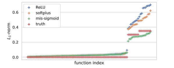
(a) Excitation scenario

(b) Inhibition scenario

Figure 21: Estimated $L_{1}$-norms after the first step of Algorithm 3, in the mis-specified settings of Simulation 6. In this simulation, the link functions are set to $\phi_{k}(x)=20\sigma(0.2(x-10)),\forall k$, in our algorithm, while the data sets are generated from a Hawkes process with ReLU, softplus, or a mis-specified sigmoid (mis-sigmoid) link functions, in Excitation and Inhibition scenarios. We note that for the ReLU and softplus link, the norms are not well estimated after the first step, nonetheless, our gap heuristic can still recover the true graph parameter.

Scenario	Link	Graph accuracy	Dimension accuracy	Risk
Excitation	ReLU	1.00	1.00	49.58
	Softplus	1.00	1.00	34.27
	Mis-specified sigmoid	1.00	1.00	19.69
Inhibition	ReLU	1.00	1.00	59.95
	Softplus	1.00	1.00	33.94
	Mis-specified sigmoid	0.99	1.00	15.78

Table 9: Performance of Algorithm 3 for the different mis-specified settings and scenarios of Simulation 6 ($K=10$). We note that the graph parameter and the dimensionality are still recovered in these cases, although, the other parameters cannot be well estimated, as can be seen from the large risk.

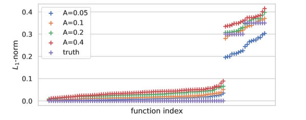
(a) Excitation scenario

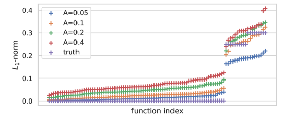
(b) Inhibition scenario

Figure 22: Estimated $L_{1}$-norms of the interaction functions after the first step of Algorithm 3 specified with different values of the memory parameter $A=0.05,0.1,0.2,0.4$ containing the true memory parameter $A_{0}=0.1$, in the scenarios of Simulation 6. In all cases, we still observe a gap, although the norms are under-estimated (resp. over-estimated)

for $A=0.05$ (resp. $A=0.4$)

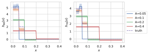
(a) Excitation scenario

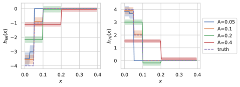
(b) Inhibition scenario

Figure 23: Model-selection variational posterior on the interaction functions $h_{66}$ and $h_{76}$ obtained with Algorithm 3, specified with different values of the memory parameter $A=0.05,0.1,0.2,0.4$, in the scenarios of Simulation 6 with $K=10$ and true memory parameter $A_{0}=0.1$. We note that the estimation of the interaction functions is deteriorated when $A$ is mis-specified, however the signs of the functions are still recovered.

6 Discussion

In this paper, we proposed a novel adaptive variational Bayes method for sparse and high-dimensional Hawkes processes, and provided a general theoretical analysis of these methods. We notably obtained variational posterior concentration rates, under easily verifiable conditions on the prior and approximating family that we validated commonly used inference set-ups. Our general theory holds in particular in the sigmoid Hawkes model, for which we developed adaptive variational mean-field algorithms, which improve existing ones by their ability to infer the graph parameter and the dimensionality of the interaction functions. Moreover, we demonstrated on simulated data that our most computationally efficient algorithm is able to scale up to high-dimensional processes.

Nonetheless, our theory does not yet cover the high-dimensional setting with $K\to\infty$, which is of interest in applications of Hawkes processes to social network analysis and neuroscience. In this limit, previous works have considered sparse models (Cai et al., 2021; Bacry et al., 2020; Chen et al., 2017a) and mean-field settings (Pfaffelhuber et al., 2022). We would therefore be interested in extending our results to these models. Moreover, our empirical study shows that the credible sets of variational distributions do not always have good coverage, an observation that sometimes also holds for the posterior distribution. Therefore, it is left for future work to study the property of (variational) posterior credible regions, and potentially design post-processing methods of the latter to improve coverage in practice. Additionally, the thresholding approach for estimating the graph in our two-step adaptive variational procedure could be further explored, in particular, in dense settings.

Finally, it would be of practical interest to develop variational algorithms beyond the sigmoid model, e.g., for the ReLU and softplus Hawkes models. While in the sigmoid model, the conjugacy of the mean-field variational posterior using data augmentation leads to particularly efficient algorithms, it is unlikely that such convenient forms could be obtained for more general models. A potential approach for other models could be to parametrise variational families with normalising flows, as it is for instance done for cut posteriors in Carmona and Nicholls (2022).

Acknowledgments and Disclosure of Funding

The project leading to this work has received funding from the European Research Council (ERC) under the European Union’s Horizon 2020 research and innovation programme (grant agreement No 834175). The project is also partially funded by the EPSRC via the CDT OxWaSP.

Appendix A Mean-field and model-selection variational inference

In this section, we first recall some general notions on mean field variational Bayes and model selection variational Bayes, then present additional details on the construction of variational families in the case of multivariate Hawkes processes.

A.1 Mean-field approximations

In a general inference context, when the parameter of interest, say $\vartheta$, is decomposed into $D$ blocks, $\vartheta=(\vartheta_{1},\dots,\vartheta_{D})$ with $D>1$, a common choice of variational class is a mean-field family that can be defined as $\mathcal{V}_{MF}=\left\{Q;\>dQ(\vartheta)=\prod_{d=1}^{D}dQ_{d}(\vartheta_{d})\right\}.$ In this case, the mean-field variational posterior distribution corresponds to $\hat{Q}=\arg\min_{Q\in\mathcal{V}_{MF}}KL\left(Q||\Pi(.|N)\right)=\prod_{d=1}^{D}\hat{Q}_{d}.$ Note that the mean-field family removes some dependencies between blocks of coordinates of the parameter in the approximated posterior distribution.

Assuming that the mean-field variational posterior distribution has a density with respect to a dominating measure $\mu=\prod_{d}\mu_{d}$, with a slight abuse of notation, we denote $\hat{Q}$ both the distribution and density with respect to $\mu$. An interesting result from Bishop (2006) is that the mean-field variational posterior distribution verifies, for each $d\in[D]$,

$$\hat{Q}_{d}(\vartheta_{d})\propto\exp\left\{\varmathbb{E}_{\hat{Q}_{-d}}[\log p(\vartheta,N)]\right\},$$ (31)

where $p(\vartheta,N)$ is the joint density of the observations and the parameter with respect to $\prod_{d}\mu_{d}\times\mu_{N}$ with $\mu_{N}$ the data density, and $\hat{Q}_{-d}:=\prod_{d^{\prime}\neq d}\hat{Q}_{d^{\prime}}$. This property (31) can be used to design efficient algorithms for computing the variational posterior, such as the coordinate-ascent variational inference algorithm.

In a general setting where the log-likelihood function of the nonlinear Hawkes model can be augmented with some latent variable $z\in\mathcal{Z}$ (see for instance Zhou et al. (2021a, 2022); Malem-Shinitski et al. (2021)), with $\mathcal{Z}$ the latent parameter space, the augmented log-likelihood $L_{T}^{A}(f,z)$ leads to an augmented posterior distribution, defined as

$$\Pi_{A}(B|N)=\frac{\int_{B}\exp(L_{T}^{A}(f,z))d(\Pi(f)\times\varmathbb{P}_{A}(z))}{\int_{\mathcal{F}\times\mathcal{Z}}\exp(L_{T}^{A}(f,z))d(\Pi(f)\times\varmathbb{P}_{A})(z)},\quad B\subset\mathcal{F}\times\mathcal{Z},$$

where $\varmathbb{P}_{A}$ is a prior distribution on $z$ which has a density with respect to a dominating measure $\mu_{z}$. Recalling the mean-field variational from Section 3.1 defined as

$$\mathcal{V}_{AMF}=\left\{Q:\mathcal{F}\times\mathcal{Z}\to[0,1];\>Q(f,z)=Q_{1}(f)Q_{2}(z)\right\},$$

the augmented mean-field variational posterior corresponds to

$$\hat{Q}_{AMF}(f,z):=\arg\min_{Q\in\mathcal{V}_{AMF}}KL\left(Q(f,z)||\Pi_{A}(f,z|N)\right)=:\hat{Q}_{1}(f)\hat{Q}_{2}(z),$$ (32)

and, using property (31), verifies

$$\hat{Q}_{1}(f)\propto\exp\left\{\varmathbb{E}_{\hat{Q}_{2}}[\log p(f,z,N)]\right\},\quad\hat{Q}_{2}(z)\propto\exp\left\{\varmathbb{E}_{\hat{Q}_{1}}[\log p(f,z,N)]\right\},$$ (33)

where $p(f,z,N)$ is the joint density of the parameter, the latent variable, and the observations with respect to the measure $\prod_{d}\mu_{d}\times\mu_{z}\times\mu_{N}$.

A.2 Model-selection variational posterior

In this section, we present two model-selection variational approaches to approximate the posterior by an adaptive variational posterior distribution. We recall from our construction in Section 3.2 that our parameter $f$ of the Hawkes processes is indexed by a model $m$ of hyperparameters in the form $m=(\delta,J_{lk},(l,k)\in\mathcal{I}(\delta))$, where $\mathcal{I}(\delta)=\{(l,k);\,\delta_{lk}=1\}$ is the set of non null functions.

In a model-selection variational approach, one can consider a set of candidate models $\mathcal{M}$ and for any $m\in\mathcal{M}$, a class of variational distributions on $f$ with model $m$, denoted $\mathcal{V}^{m}$. Then, one can define the total variational class as $\mathcal{V}=\cup_{m\in\mathcal{M}}\{\{m\}\times\mathcal{V}^{m}\}$, which contains distributions on $f$ localised on one model. Then, given $\mathcal{V}$ and as shown for instance in Zhang and Gao (2020), the variational posterior distribution has the form

$$\hat{Q} :=\hat{Q}_{\hat{m}},\quad\hat{m}:=\arg\max_{m\in\mathcal{M}}ELBO(\hat{Q}^{m}),$$

where $\hat{Q}^{m}=\arg\min_{Q\in\mathcal{V}^{m}}KL(Q|||\Pi(.|N))$ and $ELBO(\cdot)$ is called the evidence lower bound (ELBO), defined as

$$ELBO(Q) :=\varmathbb{E}_{Q}\left[\log\frac{p(f,z,N)}{Q(f,z)}\right],\quad Q\in\mathcal{V}.$$ (34)

The ELBO is a lower bound of the marginal log-likelihood $p(N)$.

An alternative model-selection variational approach consists in constructing a model-averaging variational posterior, also called adaptive in Ohn and Lin (2021), as a mixture of distributions over the different models, i.e.,

$$\hat{Q}=\sum_{m\in\mathcal{M}}\hat{\gamma}_{m}\hat{Q}_{m},$$ (35)

where $\{\hat{\gamma}_{m}\}_{m\in\mathcal{M}}$ are marginal probabilities defined as

$$\hat{\gamma}_{m}=\frac{\Pi_{m}(m)\exp\left\{ELBO(\hat{Q}_{m})\right\}}{\sum_{m\in\mathcal{M}}\Pi_{m}(m)\exp\left\{ELBO(\hat{Q}_{m})\right\}},\quad\forall m\in\mathcal{M}.$$ (36)

In this strategy, the approximating family of distributions corresponds to

$$\mathcal{V}=\left\{\sum_{m\in\mathcal{M}}\alpha_{m}Q_{m};\sum_{m}\alpha_{m}=1,\>\alpha_{m}\geqslant 0,\>Q_{m}\in\mathcal{V}^{m},\>\forall m\right\}.$$

Appendix B Data augmentation in the sigmoid Hawkes model

In this section, we recall the latent variable augmentation strategy and the definition of the augmented mean-field variational distribution in sigmoid-type Hawkes processes, proposed in previous work (Zhou et al., 2022; Malem-Shinitski et al., 2021). In our method in Section 3.2, we use this construction to efficiently compute an approximated posterior distribution on $\mathcal{F}_{m}\subset\mathcal{F}$, on parameters $f$ within a model $m=(\delta,J_{lk};(l,k)\in\mathcal{I}(\delta))$.

The first data augmentation step consists in re-writing the sigmoid function as a mixture of Polya-Gamma random variables (Polson et al., 2012), i.e.,

$$\sigma(x)=\varmathbb{E}_{\omega\sim p_{PG}(.;1,0)}\left[e^{g(\omega,x)}\right]=\int_{0}^{+\infty}e^{g(\omega,x)}p_{PG}(\omega;1,0)d\omega,\quad g(\omega,x)=-\frac{\omega x^{2}}{2}+\frac{x}{2}-\log 2,$$ (37)

with $p_{PG}(.;1,0)$ the Polya-Gamma density. We recall that $p_{PG}(.;1,0)$ is the density of the random variable

$$\frac{1}{2\pi^{2}}\sum_{k=1}^{\infty}\frac{g_{k}}{(k-1/2)^{2}},\quad g_{k}\overset{\mathrm{i.i.d.}}{\sim}Gamma(1,1),$$

and that the tilted Polya-Gamma distribution is defined as

$$p_{PG}(\omega;1,c)=\cosh{\left(\frac{c}{2}\right)}\exp\left\{-\frac{c^{2}\omega}{2}\right\}p_{PG}(\omega;1,0),\quad c\geqslant 0,$$

where $\cosh$ denotes the hyperbolic cosine function. With a slight abuse of notation, we re-define the linear intensity (2) as $\tilde{\lambda}^{k}_{t}(f)=\alpha\left(\nu_{k}+\sum_{l=1}^{K}\int_{-\infty}^{t^{-}}h_{lk}(t-s)dN_{s}^{l}-\eta\right),$ so that we have $\lambda^{k}_{t}(f)=\theta_{k}\sigma(\tilde{\lambda}^{k}_{t}(f)),t\in\varmathbb R$. For any $k\in[K]$, let $N_{k}:=N^{k}[0,T]$ and $T_{1}^{k},\dots,T_{N_{k}}^{k}\in[0,T]$ be the times of events at component $N^{k}$. Now, let $\omega=(\omega_{i}^{k})_{k\in[K],i\in[N_{k}]}$ be a set of latent variables such that

$$\omega_{i}^{k}\overset{\mathrm{i.i.d.}}{\sim}p_{PG}(\cdot;1,0),\quad i\in[N_{k}],\quad k\in[K].$$

Then, using (37), an augmented log-likelihood function can be defined as

$$L_{T}(f,\omega;N) =\sum_{k\in[K]}\left\{\sum_{i\in[N_{k}]}\left(\log\theta_{k}+g(\omega_{i}^{k},\tilde{\lambda}_{T_{i}^{k}}(f))+\log p_{PG}(\omega_{i}^{k};1,0)\right)-\int_{0}^{T}\theta_{k}\sigma(\tilde{\lambda}^{k}_{t}(f))dt\right\},$$ (38)

and, using that $\sigma(x)=1-\sigma(-x)$, the integral term on the RHS in (38) can be re-written as

$$\int_{0}^{T}\theta_{k}\sigma(\tilde{\lambda}^{k}_{t}(f))dt =\int_{0}^{T}\int_{0}^{\infty}\theta_{k}\left[1-e^{g(\bar{\omega},-\tilde{\lambda}^{k}_{t}(f))}\right]p_{PG}(\bar{\omega};1,0)d\bar{\omega}dt.$$

Secondly, Campbell’s theorem (Daley and Vere-Jones, 2007; Kingman, 1993) is applied. We first recall here its general formulation. For a Poisson point process $\bar{Z}$ on a space $\mathcal{X}$ with intensity measure $\Lambda:\mathcal{X}\to\varmathbb R^{+}$, and for any function $\zeta:\mathcal{X}\to\varmathbb R$, it holds true that

$$\operatorname*{\varmathbb{E}}\left[\prod_{x\in\bar{Z}}e^{\zeta(x)}\right]=\exp\left\{\int(e^{\zeta(x)}-1)\Lambda(dx)\right\}.$$ (39)

Therefore, using that $\sigma(x)=1-\sigma(-x)$, and considering for each $k$ a marked Poisson point process $\bar{Z}^{k}$ on $\mathcal{X}=([0,T],\varmathbb R^{+})$ with intensity measure $\Lambda^{k}(t,\omega)=\theta_{k}p_{PG}(\omega;1,0)$, and distribution $\varmathbb{P}_{\bar{Z}}$, applying Campbell’s theorem with $\zeta(t,\omega):=g(\omega,-\tilde{\lambda}^{k}_{t}(f))$, one obtains that

$$\operatorname*{\varmathbb{E}}\left[\prod_{(\bar{T}_{j}^{k},\bar{\omega}_{j}^{k})\in\bar{Z}^{k}}e^{g(\bar{\omega}_{k},-\tilde{\lambda}^{k}_{\bar{T}_{j}}(f))}\right] =\exp\left\{\int_{0}^{T}\int_{0}^{\infty}\theta_{k}\left(e^{g(\bar{\omega},-\tilde{\lambda}^{k}_{t}(f))}-1\right)p_{PG}(\bar{\omega};1,0)d\bar{\omega}dt\right\}.$$

Conditionally on $N$, let $\bar{Z}:=(\bar{Z}^{1},\dots,\bar{Z}^{K})$ be an observation of the previous Poisson point process on $[0,T]$. For each $k\in[K]$, we denote $\bar{Z}_{k}:=\bar{Z}^{k}[0,T]$, $(\bar{T}_{1}^{k},\bar{\omega}_{1}^{k}),\dots,(\bar{T}_{1}^{k},\bar{\omega}_{\bar{Z}_{k}}^{k})\in[0,T]\times\varmathbb R_{+}$ the times and marks of $\bar{Z}_{k}$, and $\bar{Z}=(\bar{Z},\omega_{i}^{k},i\leqslant N_{k},k\leqslant K)$, the set of augmented variables. Then, replacing the integral term in (38) by a product over the observation $\bar{Z}$, the doubly augmented log-likelihood function corresponds to

$$L_{T}(f,\omega,\bar{Z};N) =\sum_{k\in[K]}\left\{\sum_{i\in[N_{k}]}\left[\log\theta_{k}+g(\omega_{i}^{k},\tilde{\lambda}_{T_{i}^{k}}(f))+\log p_{PG}(\omega_{i}^{k};1,0)\right]\right.$$

$$\left.\hskip 28.45274pt+\sum_{j\in[\bar{Z}_{k}]}\left[\log\theta_{k}+g(\bar{\omega}_{j}^{k},-\tilde{\lambda}_{\bar{T}_{j}}(f))+\log p_{PG}(\bar{\omega}_{j}^{k};1,0)\right]-\theta_{k}T\right\}.$$

The previous augmented log-likelihood function, and the prior distribution $\Pi$ on the parameter and the latent variables distribution $\varmathbb{P}_{A}=p_{PG}(.|1,0)\times\varmathbb{P}_{\bar{Z}}$, allow to construct an augmented posterior distribution proportional to

$$\Pi(f,\omega,\bar{Z}|N) \propto\prod_{k}\left\{\prod_{i\in[N_{k}]}\theta_{k}e^{g(\omega_{i}^{k},\tilde{\lambda}_{T_{i}^{k}}(f))}p_{PG}(\omega_{i}^{k};1,0)\times\prod_{j\in[\bar{Z}^{k}]}\theta_{k}e^{g(\bar{\omega}_{j}^{k},-\tilde{\lambda}_{\bar{T}_{j}}(f))}p_{PG}(\bar{\omega}_{j}^{k};1,0)\right\}\times\Pi(f).$$ (40)

Appendix C Analytical derivation in the sigmoid Hawkes model

C.1 Mean-field updates in a fixed model

In this section, we derive the analytic forms of the conditional updates in Algorithm 1, the mean-field variational algorithm with fixed dimensionality described in Section 3.1. For ease of exposition, in this section we consider a model $m$ and a dimension $k$ and we drop the indices $k$ and $m$, e.g., we use the notation $Q_{1},Q_{2}$ for the variational factors. In the following computation, we use the notation $c$ to denote a generic constant which value can vary from one line to the other. For simplicity, we also assume that $J:=J_{1}=\dots=J_{K}$ and we recall that $\phi_{k}(x)=\theta_{k}\sigma(\alpha(x-\eta))$.

From the definition of the augmented posterior (40), we first note that

$$\log p(f,N,\omega,\bar{Z}) =\log\Pi(f,\omega,\bar{Z}|N)+\log p(N)=L_{T}(f,\omega,\bar{Z};N)+\log\Pi(f)+\log p(N)+c$$

$$=\log p(\omega|f,N)+\log p(\bar{Z}|f,N)+\log\Pi(f)+\log p(N)+c.$$ (41)

In the previous equality we have used the facts that $p(\omega|f,N,\bar{Z})=p(\omega|f,N)$ and $p(\bar{Z}|f,N,\omega)=p(\bar{Z}|f,N)$. We recall our notation $H(t)=(H^{0}(t),H^{1}(t),\dots,H^{K}(t))\in\varmathbb R^{KJ+1},\>t\in\varmathbb R$, where for $k\in[K]$, $H^{k}(t)=(H_{j}^{k}(t))_{j=1,\dots,J}$ and $H_{j}^{k}(t)$ is defined in (19). In the following, $H(t)$ denotes $H^{k}(t)$ for the chosen $k$. We have that

$$\varmathbb{E}_{Q_{2}}[\log p(\omega|f,N)] =\varmathbb{E}_{Q_{2}}\left[\sum_{i\in[N]}g(\omega_{i},\tilde{\lambda}_{T_{i}}(f))\right]+c=\varmathbb{E}_{Q_{2}}\left[\sum_{i\in[N]}-\frac{\omega_{i}\tilde{\lambda}_{T_{i}}(f)^{2}}{2}+\frac{\tilde{\lambda}_{T_{i}}(f)}{2}\right]+c$$

$$=\varmathbb{E}_{Q_{2}}\left[\sum_{i\in[N]}-\frac{\omega_{i}\alpha^{2}(f^{T}H(T_{i})H(T_{i})^{T}f-2\eta H(T_{i})^{T}f+\eta^{2})}{2}+\frac{\alpha H(T_{i})^{T}f}{2}\right]+c$$

$$=\varmathbb{E}_{Q_{2}}\left[-\frac{1}{2}\sum_{i\in[N]}\left\{\omega_{i}\alpha^{2}f^{T}H(T_{i})H(T_{i})^{T}f-\alpha(2\omega_{i}\alpha\eta+1)H(T_{i})^{T}f+\omega_{i}\alpha^{2}\eta^{2}\right\}\right]+c$$

$$=-\frac{1}{2}\sum_{i\in[N]}\left\{\varmathbb{E}_{Q_{2}}[\omega_{i}]\alpha^{2}f^{T}H(T_{i})H(T_{i})^{T}f-\alpha(2\varmathbb{E}_{Q_{2}}[\omega_{i}]\alpha\eta+1)H(T_{i})^{T}f+\varmathbb{E}_{Q_{2}}[\omega_{i}]\alpha^{2}\eta^{2}\right\}+c.$$

Moreover, we also have that

$$\varmathbb{E}_{Q_{2}}[\log p(\bar{Z}|f,N)] =\varmathbb{E}_{Q_{2}}\left[-\frac{1}{2}\sum_{j\in[\bar{Z}]}\left\{\bar{\omega}_{j}\alpha^{2}f^{T}H(\bar{T}_{j})H(\bar{T}_{j})^{T}f-\alpha(2\bar{\omega}_{j}\alpha\eta-1)H(\bar{T}_{j})^{T}f+\bar{\omega}_{j}\alpha^{2}\eta^{2}\right\}\right]+c$$

$$=\int_{0}^{T}\int_{0}^{\infty}\left[-\frac{1}{2}\left(\bar{\omega}\alpha^{2}f^{T}H(t)H(t)^{T}f-\alpha(2\bar{\omega}\alpha\eta-1)H(t)^{T}f+\bar{\omega}\alpha^{2}\eta^{2}\right)\right]\Lambda(t,\bar{\omega})d\bar{\omega}dt+c$$

$$=-\frac{1}{2}\left[f^{T}\left(\alpha^{2}\int_{0}^{T}\int_{0}^{\infty}\bar{\omega}H(t)H(t)^{T}\Lambda(t,\bar{\omega})d\bar{\omega}dt\right)f\right.$$

$$\hskip 28.45274pt\left.+f^{T}\left(\alpha\int_{0}^{T}\int_{0}^{\infty}(2\bar{\omega}\alpha\eta-1)H(t)^{T}\Lambda(t,\bar{\omega})d\bar{\omega}dt\right)\right]+c.$$

Besides, we have $\varmathbb{E}_{Q_{2}}[\log\Pi(f)]=-\frac{1}{2}f^{T}\Sigma^{-1}f+f^{T}\Sigma^{-1}\mu+c.$ Therefore, using (33), we obtain that

$$\log Q_{1}(f) =-\frac{1}{2}\left[f^{T}\left(\alpha^{2}\sum_{i\in[N]}\varmathbb{E}_{Q_{2}}[\omega_{i}]H(T_{i})H(T_{i})^{T}+\alpha^{2}\int_{0}^{T}\int_{0}^{\infty}\bar{\omega}H(t)H(t)^{T}\Lambda(t,\bar{\omega})d\bar{\omega}dt+\Sigma^{-1}\right)f\right.$$

$$-\left.f^{T}\left(\alpha\sum_{i\in[N]}(2\varmathbb{E}_{Q_{2}}[\omega_{i}]\alpha\eta+1)H(T_{i})^{T}+\alpha\int_{0}^{T}\int_{0}^{\infty}(2\bar{\omega}\alpha\eta-1)H(t)^{T}\Lambda(t,\bar{\omega})d\bar{\omega}dt+2\Sigma^{-1}\mu\right)\right]+c$$

$$=:-\frac{1}{2}(f-\tilde{\mu})^{T}\tilde{\Sigma}^{-1}(f-\tilde{\mu})+c,$$

therefore $Q_{1}(f)$ is a normal distribution with mean vector $\tilde{\mu}$ and covariance matrix $\tilde{\Sigma}$ given by

$$\tilde{\Sigma}^{-1}=\alpha^{2}\sum_{i\in[N]}\varmathbb{E}_{Q_{2}}[\omega_{i}]H(T_{i})H(T_{i})^{T}+\alpha^{2}\int_{0}^{T}\int_{0}^{\infty}\bar{\omega}H(t)H(t)^{T}\Lambda(t,\bar{\omega})d\bar{\omega}dt+\Sigma^{-1},$$ (42)

$$\tilde{\mu}=\frac{1}{2}\tilde{\Sigma}\left[\alpha\sum_{i\in[N]}(2\varmathbb{E}_{Q_{2}}[\omega_{i}]\alpha\eta+1)H(T_{i})^{T}+\alpha\int_{0}^{T}\int_{0}^{\infty}(2\bar{\omega}\alpha\eta-1)H(t)^{T}\Lambda(t,\bar{\omega})d\bar{\omega}dt+2\Sigma^{-1}\mu\right].$$ (43)

For $Q_{2}(\omega,\bar{Z})$, we first note that using (33) and (C.1), we have $Q_{2}(\omega,\bar{Z})=Q_{21}(\omega)Q_{22}(\bar{Z})$. Using the same computation as Donner and Opper (2019)) Appendices B and D, one can then show that

$$Q_{21}(\omega) =\prod_{i\in[N]}p_{PG}(\omega_{i}|1,\underline{\lambda}_{T_{i}}),$$

$$\underline{\lambda}_{t} =\sqrt{\varmathbb{E}_{Q_{1}}[\tilde{\lambda}_{t}(f)^{2}]}=\alpha^{2}\sqrt{H(t)^{T}\tilde{\Sigma}H(t)+(H(t)^{T}\tilde{\mu})^{2}-2\eta H(t)^{T}\tilde{\mu}+\eta^{2}},\quad\forall t\in[0,T],$$

and that $Q_{22}$ is a marked Poisson point process measure on $[0,T]\times\varmathbb R^{+}$ with intensity

$$\Lambda(t,\bar{\omega}) =\theta e^{\varmathbb{E}_{Q_{1}}[g(\bar{\omega},-\tilde{\lambda}_{t}(f)]}p_{PG}(\bar{\omega};1,0)=\theta\frac{\exp(-\frac{1}{2}\varmathbb{E}_{Q_{1}}[\tilde{\lambda}_{t}(f)])}{2\cosh\frac{\underline{\lambda}_{t}(f)}{2}}p_{PG}(\bar{\omega}|1,\underline{\lambda}_{t}(f))$$

$$=\theta\sigma(-\underline{\lambda}_{t})\exp\left\{\frac{1}{2}(\underline{\lambda}_{t}(f)-\varmathbb{E}_{Q_{1}}[\tilde{\lambda}_{t}(f)])\right\}p_{PG}(\bar{\omega}|1,\underline{\lambda}_{t})$$

$$\varmathbb{E}_{Q_{1}}[\tilde{\lambda}_{t}(f)] =\alpha(H(t)^{T}\tilde{\mu}-\eta).$$

Therefore, we have that

$$\varmathbb{E}_{Q_{1}}[\omega_{i}]=\frac{1}{2\underline{\lambda}_{T_{i}}}\tanh\left(\frac{\underline{\lambda}_{T_{i}}}{2}\right),\quad\forall i\in[N].$$

C.2 Analytic formulas of the ELBO

In this section, we provide the derivation of the evidence lower bound $(ELBO(\hat{Q}_{k}^{m}))_{k}$ for a mean-field variational distribution $\hat{Q}_{m}(f,\bar{Z})=\hat{Q}_{1}^{m}(f)\hat{Q}_{2}^{m}(\bar{Z})$ in a fixed model $m=(\delta,D)$. For ease of exposition, we drop the subscript $m$ and $k$. From (34), we have

$$ELBO(\hat{Q}) =\varmathbb{E}_{\hat{Q}}\left[\log\frac{p(f,\omega,\bar{Z},N)}{\hat{Q}_{1}(f)\hat{Q}_{2}(\omega,\bar{Z})}\right]$$

$$=\varmathbb{E}_{\hat{Q}_{2}}\left[-\log\hat{Q}_{2}(\omega,\bar{Z})\right]+\varmathbb{E}_{\hat{Q}_{2}}\left[\varmathbb{E}_{\hat{Q}_{1}}\left[\log p(f,\omega,\bar{Z},N)\right]\right]+\varmathbb{E}_{\hat{Q}_{1}}[-\log\hat{Q}_{1}(f)].$$

Now using the notation of Section 3.1, we first note that defining $K(t):=H(t)H(t)^{T}$, we have that

$$\varmathbb{E}_{\hat{Q}_{1}}[\tilde{\lambda}_{T_{i}}(f)^{2}]=tr(K(t)\tilde{\Sigma})+\tilde{\mu}^{T}K(t)\tilde{\mu}$$

$$\varmathbb{E}_{\hat{Q}_{1}}\left[\log\mathcal{N}(f;\mu,\Sigma)\right]=-\frac{1}{2}tr(\Sigma^{-1}\tilde{\Sigma})-\frac{1}{2}\tilde{\mu}^{T}\Sigma^{-1}\tilde{\mu}+\tilde{\mu}^{T}\Sigma^{-1}\mu-\frac{1}{2}\mu^{T}\Sigma^{-1}\mu-\frac{1}{2}\log|2\pi\Sigma|.$$

Moreover, we have

$$\varmathbb{E}_{\hat{Q}_{1}}[\log\hat{Q}_{1}(f)] =-\frac{|m|}{2}-\frac{1}{2}\log|2\pi\tilde{\Sigma}|.$$

Using that for any $c>0$, $p_{PG}(\omega;1,c)=e^{-c^{2}\omega/2}\cosh{(c/2)}p_{PG}(\omega;1,0),$ we also have

$$\varmathbb{E}_{\hat{Q}_{2}}\left[-\log\hat{Q}_{2}(\omega,\bar{Z})\right] =\sum_{i\in[N]}-\varmathbb{E}_{\hat{Q}_{2}}[\log p_{PG}(\omega_{i},1,0)]+\frac{1}{2}\varmathbb{E}_{\hat{Q}_{2}}[\omega_{i}]\varmathbb{E}_{\hat{Q}_{1}}[\tilde{\lambda}_{T_{i}}(f)^{2}]-\log\cosh{\left(\frac{\underline{\lambda}_{T_{i}}(f)}{2}\right)}$$

$$-\int_{t=0}^{T}\int_{0}^{+\infty}[\log\Lambda(t,\bar{\omega})]\Lambda(t,\bar{\omega})d\bar{\omega}dt+\int_{t=0}^{T}\int_{0}^{+\infty}\Lambda(t,\bar{\omega})d\bar{\omega}dt$$

$$=\sum_{i\in[N]}-\varmathbb{E}_{\hat{Q}_{2}}[\log p_{PG}(\omega_{i},1,0)]+\frac{1}{2}\varmathbb{E}_{\hat{Q}_{2}}[\omega_{i}]\varmathbb{E}_{\hat{Q}_{1}}[\tilde{\lambda}_{T_{i}}(f)^{2}]-\log\cosh{\left(\frac{\underline{\lambda}_{T_{i}}(f)}{2}\right)}$$

$$-\int_{t=0}^{T}\int_{0}^{+\infty}\left[\log\theta-\frac{1}{2}\varmathbb{E}_{\hat{Q}_{1}}[\tilde{\lambda}_{T_{i}}(f)]-\log 2-\log\cosh{\left(\frac{\underline{\lambda}_{T_{i}}(f)}{2}\right)}-\frac{1}{2}\varmathbb{E}_{\hat{Q}_{1}}[\tilde{\lambda}_{T_{i}}(f)^{2}]\bar{\omega}\right.$$

$$+\left.\log\cosh{\left(\frac{1}{2}\underline{\lambda}_{T_{i}}(f)\right)}+\log p_{PG}(\bar{\omega};1,0)-1\right]\Lambda(t)p_{PG}(\bar{\omega};1,\underline{\lambda}_{T_{i}}(f))dtd\bar{\omega}$$

$$=\sum_{i\in[N]}-\varmathbb{E}_{\hat{Q}_{2}}[\log p_{PG}(\omega_{i},1,0)]+\frac{1}{2}\varmathbb{E}_{\hat{Q}_{2}}[\omega_{i}^{k}]\varmathbb{E}_{\hat{Q}_{1}}[\tilde{\lambda}_{T_{i}}(f)^{2}]-\log\cosh{\left(\frac{\underline{\lambda}_{T_{i}}(f)}{2}\right)}$$

$$-\int_{t=0}^{T}\left[\log\theta-\frac{1}{2}\varmathbb{E}_{\hat{Q}_{1}}[\tilde{\lambda}_{T_{i}}(f)]-\log 2-\frac{1}{2}\varmathbb{E}_{\hat{Q}_{1}}[\tilde{\lambda}_{T_{i}}(f)^{2}]\varmathbb{E}_{\hat{Q}_{2}}[\bar{\omega}]-1\right]\Lambda(t)dt$$

$$-\int_{t=0}^{T}\int_{0}^{+\infty}\log p_{PG}(\omega;1,0)\Lambda(t)p_{PG}(\omega;1,\underline{\lambda}_{T_{i}}(f))d\omega dt.$$

with $\Lambda(t)=\theta\int_{0}^{\infty}\Lambda(t,\bar{\omega})d\bar{\omega}=\frac{e^{-\frac{1}{2}\varmathbb{E}_{\hat{Q}_{1}}[\tilde{\lambda}_{T_{i}}(f)]}}{2\cosh\frac{\underline{\lambda}_{T_{i}}(f)}{2}}$. Moreover, we have

$$\varmathbb{E}_{\hat{Q}_{2}}\left[\varmathbb{E}_{\hat{Q}_{1}}\left[\log p(f,\omega,\bar{Z},N)\right]\right]=\sum_{i\in[N]}\left\{\log\theta+\varmathbb{E}_{\hat{Q}_{2}}\left[\varmathbb{E}_{\hat{Q}_{1}}\left[g(\omega_{i},\tilde{\lambda}_{T_{i}}(f))\right]+\log p_{PG}(\omega_{i};1,0)\right]\right\}$$

$$+\log\theta+\varmathbb{E}_{\hat{Q}_{2}}\left[\varmathbb{E}_{\hat{Q}_{1}}\left[g(\bar{\omega}_{t},-\tilde{\lambda}_{T_{i}}(f)))\right]+\log p_{PG}(\bar{\omega}_{t};1,0)\right]+\varmathbb{E}_{\hat{Q}_{1}}\left[\log\mathcal{N}(f;\mu,\Sigma)\right]$$

$$=\sum_{i\in[N]}\log\theta-\log 2-\frac{1}{2}\varmathbb{E}_{\hat{Q}_{1}}\left[\tilde{\lambda}_{T_{i}}(f)^{2}\right]\varmathbb{E}_{\hat{Q}_{2}}\left[\omega_{i}\right]+\frac{1}{2}\varmathbb{E}_{\hat{Q}_{1}}\left[\tilde{\lambda}_{T_{i}}(f)\right]+\varmathbb{E}_{\hat{Q}_{2}}\left[\log p_{PG}(\omega_{i};1,0)\right]$$

$$+\int_{0}^{T}\int_{0}^{+\infty}\left[\log\theta_{k}-\log 2-\frac{1}{2}\varmathbb{E}_{\hat{Q}_{1}}\left[\tilde{\lambda}_{T_{i}}(f)^{2}\right]\bar{\omega}-\frac{1}{2}\varmathbb{E}_{\hat{Q}_{1}}\left[\tilde{\lambda}_{T_{i}}(f)\right]+\log p_{PG}(\bar{\omega};1,0)\right]\Lambda^{k}(t)p_{PG}(\omega;1,\underline{\lambda}_{T_{i}}(f))d\omega dt$$

$$+\varmathbb{E}_{\hat{Q}_{1}}\left[\log\mathcal{N}(f;\mu,\Sigma)\right]-\theta T$$

$$=\sum_{i\in[N]}\log\theta_{k}-\log 2-\frac{1}{2}\varmathbb{E}_{\hat{Q}_{1}}\left[\tilde{\lambda}_{T_{i}}(f)^{2}\right]\varmathbb{E}_{\hat{Q}_{2}}\left[\omega_{i}\right]+\frac{1}{2}\varmathbb{E}_{\hat{Q}_{1}}\left[\tilde{\lambda}_{T_{i}}(f)\right]+\varmathbb{E}_{\hat{Q}_{2}}\left[\log p_{PG}(\omega_{i};1,0)\right]$$

$$+\int_{0}^{T}\left[\log\theta-\log 2-\frac{1}{2}\varmathbb{E}_{\hat{Q}_{1}}\left[\tilde{\lambda}_{T_{i}}(f)^{2}\right]\varmathbb{E}_{\hat{Q}_{2}}\left[\bar{\omega}\right]-\frac{1}{2}\varmathbb{E}_{\hat{Q}_{1}}\left[\tilde{\lambda}_{T_{i}}(f)\right]\right]\Lambda(t)dt$$

$$+\int_{0}^{T}\int_{0}^{+\infty}\log p_{PG}(\bar{\omega};1,0)\Lambda(t)p_{PG}(\bar{\omega};1,\underline{\lambda}_{T_{i}}(f))d\bar{\omega}dt+\varmathbb{E}_{\hat{Q}_{1}}\left[\log\mathcal{N}(f;\mu,\Sigma)\right]-\theta T.$$

Therefore, with $c>0$ a constant that does not depend on the size of the model, with zero mean prior $\mu=0$,

$$ELBO(\hat{Q}) =\frac{|m|}{2}+\frac{1}{2}\log|2\pi\tilde{\Sigma}|-\frac{1}{2}tr(\Sigma^{-1}\tilde{\Sigma})-\frac{1}{2}\tilde{\mu}^{T}\Sigma^{-1}\tilde{\mu}-\frac{1}{2}\log|2\pi\Sigma|$$

$$+\sum_{i\in[N]}\log\theta-\log 2+\frac{\varmathbb{E}_{\hat{Q}_{1}}\left[\tilde{\lambda}_{T_{i}}(f)\right]}{2}-\log\cosh\left(\frac{\tilde{\lambda}_{T_{i}}(f)}{2}\right)$$

$$+\int_{t=0}^{T}\int_{0}^{+\infty}\Lambda(t,\bar{\omega})d\bar{\omega}dt-\theta T.$$

C.3 Gibbs sampler

From the augmented posterior $\Pi_{A}(f,\omega,\bar{|}N)$ defined in (40) and using the Gaussian prior family described in Section 3.1, similar computation as Appendix C.1 can provide analytic forms of the conditional posterior distributions $\Pi_{A}(f|\omega,\bar{Z},N),\Pi_{A}(\omega|N,f)$ and $\Pi_{A}(\bar{Z}|f,N)$ . This allows to design a Gibbs sampler algorithm that sequentially samples the parameter $f$, the latent variables $\omega$ and Poisson process $\bar{Z}$. With the notation of Appendix C.1, such procedure can be defined as

For every $k\in[K]$,

(Sample latent variables) $$\omega^{k}_{i}|N,f_{k}\sim p_{PG}(\omega_{i}^{k};1,\tilde{\lambda}^{k}_{T_{i}^{k}}(f)),\quad\forall i\in[N_{k}]$$

$$\bar{Z}^{k}|f_{k} [0,T]$$, a Poisson process on with intensity

$$\Lambda^{k}(t,\bar{\omega})=\theta_{k}\sigma(-\tilde{\lambda}^{k}_{t}(f))p_{PG}(\bar{\omega};1,\tilde{\lambda}_{t}^{k}(f))$$

(Update hyperparameters) $$R_{k}=\bar{N}^{k}[0,T]$$

$$H_{k}=[H_{N^{k}},H_{\bar{Z}^{k}}],\>[H_{N^{k}}]_{id}=H_{j}(T_{i}^{k}),$$

$$[H_{\bar{Z}^{k}}]_{jd}=H_{b}(\bar{T}_{j}^{k}),\>d=0,\dots,KJ,\>i\in[N_{k}],\>j\in[R_{k}]$$

$$D_{k}=Diag([\omega^{k}_{i}]_{i\in[N^{k}]},[\bar{\omega}^{k}_{j}]_{j\in[R^{k}]})$$

$$\tilde{\Sigma}_{k}=[\beta^{2}H_{k}D_{k}(H_{k})^{T}+\Sigma^{-1}]^{-1}$$

$$\tilde{\mu}_{k}=\tilde{\Sigma}_{k}\left(H_{k}\left[\beta v_{k}+\beta^{2}\eta u_{k}\right]+\Sigma^{-1}\mu\right),$$

$$\quad v_{k}=0.5[\mathds{1}_{N_{k}},-\mathds{1}_{R_{k}}],\quad u_{k}=[[\omega^{k}_{i}]_{i\in[N_{k}]},[\bar{\omega}^{k}_{j}]_{j\in[R_{k}]}]$$

(Sample parameter) $$f_{k}|N,\bar{Z}^{k},\omega^{k}\sim\mathcal{N}(f_{k};\tilde{m}_{k},\tilde{\Sigma}_{k}).$$

These steps are summarised in Algorithm 4 in Appendix. We note that in this algorithm, one does not need to perform a numerical integration, however, sampling the latent Poisson process is computationally intensive. In our numerical experiments, we use the Python package polyagamma to sample the Polya-Gamma variables and a thinning algorithm to sample the inhomogeneous Poisson process.

Appendix D Proofs

In this section, we provide the proof of our main theoretical result, namely Theorem 6. We first recall a set of useful lemmas from Sulem et al. (2021).

D.1 Technical lemmas

In the first lemma, we recall the definition of excursions from Sulem et al. (2021), for stationary nonlinear Hawkes processes verifying conditions (C1) or (C2). Then, Lemma 13, corresponding to Lemma A.1 in Sulem et al. (2021), provides a control on the main event $\tilde{\Omega}_{T}$ considered in the proof of Theorem 6. Finally, Lemma 14 (Lemma A.4 in Sulem et al. (2021)) is a technical lemma for proving posterior concentration in Hawkes processes.

We also introduce the following notation. For any excursion index $j\in[J_{T}-1]$, we denote $(U_{j}^{(1)},U_{j}^{(2)})$ the times of the first two events after the $j$-th renewal time $\tau_{j}$, and $\xi_{j}:=U_{j}^{(2)}$ if $U_{j}^{(2)}\in[\tau_{j},\tau_{j+1})$ and $\xi_{j}:=\tau_{j+1}$ otherwise.

Lemma 12 (Lemma 5.1 in Sulem et al. (2021))

Let $N$ be a Hawkes process with monotone non-decreasing and Lipschitz link functions $\phi=(\phi_{k})_{k}$ and parameter $f=(\nu,h)$ such that $(\phi,f)$ verify (C1) or (C2). Then the point process measure $X_{t}(.)$ defined as

$$X_{t}(.)=N|_{(t-A,t]},$$ (44)

is a strong Markov process with positive recurrent state $\emptyset$. Let $\{\tau_{j}\}_{j\geqslant 0}$ be the sequence of random times defined as

$$\tau_{j}=\begin{cases}0&\text{ if }j=0;\\ \inf\left\{t>\tau_{j-1};\>X_{t^{-}}\neq\emptyset,\>X_{t}=\emptyset\right\}=\inf\left\{t>\tau_{j-1};\>N|_{[t-A,t)}\neq\emptyset,\>N|_{(t-A,t]}=\emptyset\right\}&\text{ if }j\geqslant 1.\end{cases}$$

Then, $\{\tau_{j}\}_{j\geqslant 0}$ are stopping times for the process $N$. For $T>0$, we also define

$$J_{T}=\max\{j\geqslant 0;\>\tau_{j}\leqslant T\}.$$ (45)

The intervals $\{[\tau_{j},\tau_{j+1})\}_{j=0}^{J_{T}-1}\cup[\tau_{J_{T}},T]$ form a partition of $[0,T]$. The point process measures $(N|_{[\tau_{j},\tau_{j+1})})_{1\leqslant j\leqslant J_{T}-1}$ are i.i.d. and independent of $N|_{[0,\tau_{1})}$ and $N|_{[\tau_{J_{T}},T]}$; they are called excursions and the stopping times $\{\tau_{j}\}_{j\geqslant 1}$ are called regenerative or renewal times.

Lemma 13 (Lemma A.1 in Sulem et al. (2021))

Let $Q>0$. We consider $\tilde{\Omega}_{T}$ defined in Section D.2. For any $\beta>0$, we can choose $C_{\beta}$ and $c_{\beta}$ in the definition of $\tilde{\Omega}_{T}$ such that $\varmathbb{P}_{0}[\tilde{\Omega}_{T}^{c}]\leqslant T^{-\beta}.$ Moreover, for any $1\leqslant q\leqslant Q$,

$$\varmathbb{E}_{0}\left[\mathds{1}_{\tilde{\Omega}_{T}^{c}}\max_{l}\sup\limits_{t\in[0,T]}\left(N^{l}[t-A,t)\right)^{q}\right]\leqslant 2T^{-\beta/2}.$$

Lemma 14 (Lemma A.4 in Sulem et al. (2021))

For any $f\in\mathcal{F}_{T}$ and $l\in[K]$, let

$$Z_{1l}=\int_{\tau_{1}}^{\xi_{1}}|\lambda^{l}_{t}(f)-\lambda^{l}_{t}(f_{0})|dt.$$

Under the assumptions of Theorem 6, for $M_{T}\to\infty$ such that $M_{T}>M\sqrt{\kappa_{T}}$ with $M>0$ and for any $f\in\mathcal{F}_{T}$ such that $\left\lVert r-r_{0}\right\rVert_{1}\leqslant\max(\left\lVert r_{0}\right\rVert_{1},\tilde{C})$ with $\tilde{C}>0$, there exists $l\in[K]$ such that on $\tilde{\Omega}_{T}$,

$$\varmathbb{E}_{f}\left[Z_{1l}\right]\geqslant C(f_{0})\Big{(}\left\lVert r_{f}-r_{0}\right\rVert_{1}+\left\lVert h-h_{0}\right\rVert_{1}\Big{)},$$

with $C(f_{0})>0$ a constant that depends only on $f_{0}$ and $(\phi_{k})_{k}$.

D.2 Proof of Theorem 6

We recall that in this result, we consider a general Hawkes model with known link functions $(\phi_{k})_{k}$. Let $r_{0}=(r_{1}^{0},\dots,r_{K}^{0})$ with $r_{k}^{0}=\phi_{k}(\nu_{k}^{0})$. With $C_{\beta},c_{\beta}>0$, we first define $\tilde{\Omega}_{T}\in\mathcal{G}_{T}$ as

$$\tilde{\Omega}_{T} =\Omega_{N}\cap\Omega_{J}\cap\Omega_{U},$$

$$\Omega_{N} =\left\{\max\limits_{k\in[K]}\sup\limits_{t\in[0,T]}N^{k}[t-A,t)\leqslant C_{\beta}\log T\right\}\cap\left\{\sum_{k=1}^{K}\left|\frac{N^{k}[-A,T]}{T}-\mu_{k}^{0}\right|\leqslant\delta_{T}\right\},$$

$$\Omega_{J} =\left\{J_{T}\in\mathcal{J}_{T}\right\},\quad\Omega_{U}=\left\{\sum_{j=1}^{J_{T}-1}(U_{j}^{(1)}-\tau_{j})\geqslant\frac{T}{\varmathbb{E}_{0}[\Delta\tau_{1}]\|r_{0}\|_{1}}\left(1-2c_{\beta}\sqrt{\frac{\log T}{T}}\right)\right\},$$

$$\mathcal{J}_{T} =\left\{J\in{\varmathbb N};\>\left|\frac{J-1}{T}-\frac{1}{\varmathbb{E}_{0}[\Delta\tau_{1}]}\right|\leqslant c_{\beta}\sqrt{\frac{\log T}{T}}\right\},$$

with $J_{T}$ the number of excursions as defined in (45), $\mu_{k}^{0}:=\varmathbb{E}_{0}\left[\lambda_{t}^{k}(f_{0})\right],\forall k$, $\delta_{T}=\delta_{0}\sqrt{\frac{\log T}{T}},\>\delta_{0}>0$ and $\{U_{j}^{(1)}\}_{j=1,\dots,J_{T}-1}$ denoting the first events of each excursion (see Lemma 12 for a precise definition). Secondly, we define $A_{T}^{\prime}\in\mathcal{G}_{T}$ as

$$A_{T}^{\prime}=\left\{\int e^{L_{T}(f)-L_{T}(f_{0})}d\widetilde{\Pi}(f)>e^{-C_{1}T\epsilon_{T}^{2}}\right\},\quad\widetilde{\Pi}(B)=\frac{\Pi(B\cap K_{T})}{\Pi(K_{T})},\quad K_{T}\subset\mathcal{F},$$

with $C_{1}>0$ and $\epsilon_{T},M_{T}$ positive sequences such that $T\epsilon_{T}^{2}\to\infty$ and $M_{T}\to\infty$. From Lemma 13, we have that $\varmathbb{P}_{0}\left[\tilde{\Omega}_{T}^{c}\right]=o(1)$. Thus, with $D_{T}$ defined in (4), $A_{T}=\tilde{\Omega}_{T}\cap A_{T}^{\prime}$, $K_{T}=B_{\infty}(\epsilon_{T})$, and $\epsilon_{T}=\sqrt{\kappa_{T}}\epsilon_{T}$, we obtain that

$$\varmathbb{P}_{0}\left[A_{T}^{c}\right] \leqslant\varmathbb{P}_{0}\left[\tilde{\Omega}_{T}^{c}\right]+\varmathbb{P}_{0}\left[A_{T}^{\prime c}\cap\tilde{\Omega}_{T}\right]$$

$$=o(1)+\varmathbb{P}_{0}\left[\left\{\int_{K_{T}}e^{L_{T}(f)-L_{T}(f_{0})}d\Pi(f)\leqslant\Pi(K_{T})e^{-C_{1}T\epsilon_{T}^{2}}\right\}\cap\tilde{\Omega}_{T}\right]$$

$$\leqslant o(1)+\varmathbb{P}_{0}\left[\left\{D_{T}\leqslant\Pi(K_{T})e^{-C_{1}T\epsilon_{T}^{2}}\right\}\cap\tilde{\Omega}_{T}\right]=o(1),$$

with $C_{1}>1$, using (A0), i.e., $\Pi(K_{T})\geqslant e^{-c_{1}T\epsilon_{T}^{2}}$, and the following intermediate result from the proof of Theorem 3.2 in Sulem et al. (2021)

$$\varmathbb{P}_{0}\left[\left\{D_{T}\leqslant\Pi(B_{\infty}(\epsilon_{T}))e^{-\kappa_{T}T\epsilon_{T}^{2}}\right\}\cap\tilde{\Omega}_{T}\right]=o(1).$$

Therefore, we can conclude that

$$\varmathbb{P}_{0}\left[A_{T}\right]\xrightarrow[T\to\infty]{}1.$$

We now define the stochastic distance $\tilde{d}_{1T}$ and stochastic neighborhoods around $f_{0}$ as

$$\tilde{d}_{1T}(f,f^{\prime})=\frac{1}{T}\sum_{k=1}^{K}\int_{0}^{T}\mathds{1}_{A_{2}(T)}(t)|\lambda_{t}^{k}(f)-\lambda_{t}^{k}(f^{\prime})|dt,\quad A_{2}(T)=\bigcup_{j=1}^{J_{T}-1}[\tau_{j},\xi_{j}]$$ (46)

$$A_{d_{1}}(\epsilon)=\left\{f\in\mathcal{F};\>\tilde{d}_{1T}(f,f_{0})\leqslant\epsilon\right\},\quad\epsilon>0,$$

where for each $j\in[J_{T}]$, $U_{j}^{(2)}$ is the first event after $U_{j}^{(1)}$, and $\xi_{j}:=U_{j}^{(2)}$ if $U_{j}^{(2)}\in[\tau_{j},\tau_{j+1})$ and $\xi_{j}:=\tau_{j+1}$ otherwise. Let $\eta_{T}$ be a positive sequence and $\hat{Q}$ be the variational posterior as defined in (8). We have

$$\varmathbb{E}_{0}\left[\hat{Q}(A_{d_{1}}(\eta_{T})^{c})\right] \leqslant\varmathbb{P}_{0}\left[A_{T}^{c}\right]+\varmathbb{E}_{0}\left[\hat{Q}(A_{d_{1}}(\eta_{T})^{c})\mathds{1}_{A_{T}}\right].$$ (47)

We first bound the second term on the RHS of (47) using the following technical lemma, which is an adaptation of Theorem 5 of Ray and Szabó (2021) and Lemma 13 in Nieman et al. (2021).

Lemma 15

Let $B_{T}\subset\mathcal{F}$, $A_{T}\in\mathcal{G}_{T}$, and $Q$ be a distribution on $\mathcal{F}$. If there exist $C,u_{T}>0$ such that

$$\varmathbb{E}_{0}\left[\Pi(B_{T}|N)\mathds{1}_{A_{T}}\right]\leqslant Ce^{-u_{T}},$$ (48)

then, we have that

$$\varmathbb{E}_{0}\left[Q(B_{T})\mathds{1}_{A_{T}}\right]\leqslant\frac{2}{u_{T}}\left(\varmathbb{E}_{0}\left[KL(Q||\Pi(.|N))\mathds{1}_{A_{T}}\right]+Ce^{-u_{T}/2}\right).$$

Proof  We follow the proof of Ray and Szabó (2021) and use the fact that, for any $g:\mathcal{F}\to\varmathbb R$ such that $\int_{\mathcal{F}}e^{g(f)}d\Pi(f|N)<+\infty$, it holds true that

$$\int_{\mathcal{F}}g(f)dQ(f)\leqslant KL(Q||\Pi(.|N))+\log\int_{\mathcal{F}}e^{g(f)}\Pi(f|N).$$

Applying the latter inequality with $g=\frac{1}{2}u_{T}\mathds{1}_{B_{T}}$, we obtain

$$\frac{1}{2}u_{T}Q(B_{T}) \leqslant KL(Q||\Pi(.|N))+\log(1+e^{\frac{1}{2}u_{T}}\Pi(B_{T}|N))$$

$$\leqslant KL(Q||\Pi(.|N))+e^{\frac{1}{2}u_{T}}\Pi(B_{T}|N).$$

Then, multiplying both sides of the previous inequality by $\mathds{1}_{A_{T}}$ and taking expectation w.r.t. to $\varmathbb{P}_{0}$, using (48), we finally obtain

$$\frac{1}{2}u_{T}\varmathbb{E}_{0}\left[Q(B_{T})\mathds{1}_{A_{T}}\right]\leqslant\varmathbb{E}_{0}\left[KL(Q||\Pi(.|N))\mathds{1}_{A_{T}}\right]+Ce^{-\frac{1}{2}u_{T}}.$$

 
We thus apply Lemma 15 with $B_{T}=A_{d_{1}}(\eta_{T})^{c}$, $\eta_{T}=M_{T}^{\prime}\epsilon_{T}$, $Q=\hat{Q}$, and $u_{T}=M_{T}T\epsilon_{T}^{2}$ with $M_{T}^{\prime}\to\infty$. We first check that (48) holds, i.e., we show that there exist $C,M_{T},M_{T}^{\prime}>0$ such that

$$\varmathbb{E}_{0}\left[\mathds{1}_{A_{T}}\Pi[\tilde{d}_{1T}(f,f_{0})>M_{T}^{\prime}\epsilon_{T}|N]\right]\leqslant C\exp(-M_{T}T\epsilon_{T}^{2}).$$ (49)

For any test $\phi$, we have the following decomposition

$$\varmathbb{E}_{0}\left[\mathds{1}_{A_{T}}\Pi[\tilde{d}_{1T}(f,f_{0})>M_{T}^{\prime}\epsilon_{T}|N]\right]\leqslant\underbrace{\varmathbb{E}_{0}\left[\phi\mathds{1}_{A_{T}}]\right]}_{(I)}+\underbrace{\varmathbb{E}_{0}\left[(1-\phi)\mathds{1}_{A_{T}}\Pi[A_{d_{1}}(M_{T}^{\prime}\epsilon_{T})^{c}|N]\right]}_{(II)}.$$

Note that we have

$$(II)=\varmathbb{E}_{0}\left[(1-\phi)\mathds{1}_{A_{T}}\Pi[A_{d_{1}}(M_{T}^{\prime}\epsilon_{T})^{c}|N]\right] =\varmathbb{E}_{0}\left[\int_{A_{d_{1}}(M_{T}^{\prime}\epsilon_{T})^{c}}\mathds{1}_{A_{T}}(1-\phi)\frac{e^{L_{T}(f)-L_{T}(f_{0})}}{D_{T}}d\Pi(f)\right]$$

$$\leqslant\frac{e^{C_{1}T\epsilon_{T}^{2}}}{\Pi(K_{T})}\varmathbb{E}_{0}\left[\sup_{f\in\mathcal{F}_{T}}\varmathbb{E}_{f}\left[\mathds{1}_{A_{d_{1}}(M_{T}^{\prime}\epsilon_{T})^{c}}\mathds{1}_{A_{T}}(1-\phi)|\mathcal{G}_{0}\right]\right],$$ (50)

since on $A_{T},D_{T}\geqslant\Pi(K_{T})e^{-C_{1}T\epsilon_{T}^{2}}$. Using the proof of Theorem 5.5 in Sulem et al. (2021), we can directly obtain that for $T$ large enough, there exist $x_{1},M,M^{\prime}>0$ such that

$$(I)\leqslant 2(2K+1)e^{-x_{1}{M^{\prime}_{T}}^{2}T\epsilon_{T}^{2}}$$

$$(II)\leqslant 2(2K+1)e^{-x_{1}{M^{\prime}_{T}}^{2}T\epsilon_{T}^{2}/2},$$

which implies that

$$\varmathbb{E}_{0}\left[\mathds{1}_{A_{T}}\Pi[\tilde{d}_{1T}(f,f_{0})>M_{T}^{\prime}\epsilon_{T}|N]\right] \leqslant 4(2K+1)e^{-x_{1}M_{T}^{\prime 2}T\epsilon_{T}^{2}/2},$$

and (49) with $M_{T}=x_{1}M_{T}^{\prime 2}/2$ and $C=4(2K+1)$. Applying Lemma 15 thus leads to

$$\varmathbb{E}_{0}\left[\hat{Q}(A_{d_{1}}(\eta_{T})^{c})\mathds{1}_{A_{T}}\right]\leqslant 2\frac{KL(\hat{Q}||\Pi(.|N))+Ce^{-M_{T}T\epsilon_{T}^{2}/2}}{M_{T}T\epsilon_{T}^{2}}\leqslant 2Ce^{-M_{T}T\epsilon_{T}^{2}/2}+2\frac{KL(\hat{Q}||\Pi(.|N))}{M_{T}T\epsilon_{T}^{2}}.$$

Moreover, from (A2) and the remark following Theorem 6, it holds that $KL(\hat{Q}||\Pi(.|N))=O(T\epsilon_{T}^{2})$, therefore we obtain the following intermediate result

$$\varmathbb{E}_{0}\left[\hat{Q}(A_{d_{1}}(\eta_{T})^{c})\right]=o(1).$$

Now, with $M_{T}>M_{T}^{\prime}$, we note that

$$\varmathbb{E}_{0}\left[\hat{Q}(\left\lVert f-f_{0}\right\rVert_{1}>M_{T}\epsilon_{T})\right] =\varmathbb{E}_{0}\left[\hat{Q}(\tilde{d}_{1T}(f,f_{0})>M_{T}^{\prime}\epsilon_{T})\right]$$

$$\hskip 14.22636pt+\varmathbb{E}_{0}\left[\hat{Q}(\left\lVert f-f_{0}\right\rVert_{1}>M_{T}\epsilon_{T},\tilde{d}_{1T}(f,f_{0})<M_{T}^{\prime}\epsilon_{T})\mathds{1}_{A_{T}}\right]+\varmathbb{P}_{0}[A_{T}^{c}].$$

Therefore, it remains to show that

$$\varmathbb{E}_{0}\left[\hat{Q}(\left\lVert f-f_{0}\right\rVert_{1}>M_{T}\epsilon_{T},\tilde{d}_{1T}(f,f_{0})<M_{T}^{\prime}\epsilon_{T})\mathds{1}_{A_{T}}\right]=\varmathbb{E}_{0}\left[\hat{Q}(A_{L_{1}}(M_{T}\epsilon_{T})^{c}\cap A_{d_{1}}(M_{T}^{\prime}\epsilon_{T}))\mathds{1}_{A_{T}}\right]=o(1).$$

For this, we apply again Lemma 15 with $B_{T}=A_{L_{1}}(M_{T}\epsilon_{T})^{c}\cap A_{d_{1}}(M_{T}^{\prime}\epsilon_{T})$ and $u_{T}=TM_{T}^{2}\epsilon_{T}^{2}$. We have

$$\varmathbb{E}_{0}\left[\mathds{1}_{A_{T}}\Pi(A_{L_{1}}(M_{T}\epsilon_{T})^{c}\cap A_{d_{1}}(M_{T}^{\prime}\epsilon_{T})|N)\right] \leqslant\frac{e^{C_{1}T\epsilon_{T}^{2}}}{\Pi(K_{T})}\varmathbb{E}_{0}\left[\varmathbb{E}_{f}\left[\mathds{1}_{A_{T}}\mathds{1}_{A_{L_{1}}(M_{T}\epsilon_{T})^{c}\cap A_{d_{1}}(M_{T}^{\prime}\epsilon_{T})}|\mathcal{G}_{0}\right]\right].$$

Let $f\in A_{L_{1}}(M_{T}\epsilon_{T})^{c}\cap A_{d_{1}}(M_{T}^{\prime}\epsilon_{T})$. For any $j\in[J_{T}-1]$ and $l\in[K]$, let

$$Z_{jl}=\int_{\tau_{j}}^{\xi_{j}}|\lambda^{l}_{t}(f)-\lambda^{l}_{t}(f_{0})|dt,\quad j\in[J_{T}-1],\quad l\in[K].$$ (51)

Using Lemma 14 and the integer $l$ introduced in this lemma, for any $f\in A_{L_{1}}(M_{T}\epsilon_{T})^{c}$, we have

$$\varmathbb{E}_{f}\left[\mathds{1}_{A_{T}}\mathds{1}_{A_{d_{1}}(M_{T}^{\prime}\epsilon_{T})}|\mathcal{G}_{0}\right] \leqslant\varmathbb{P}_{f}\left[\sum_{j=1}^{J_{T}-1}Z_{jl}\leqslant TM_{T}^{\prime}\epsilon_{T}|\mathcal{G}_{0}\right]$$

$$\leqslant\sum_{J\in\mathcal{J}_{T}}\varmathbb{P}_{f}\left[\sum_{j=1}^{J-1}Z_{jl}-\varmathbb{E}_{f}\left[Z_{jl}\right]\leqslant TM_{T}^{\prime}\epsilon_{T}-\frac{T}{2\varmathbb{E}_{0}\left[\Delta\tau_{1}\right]}C(f_{0})M_{T}\epsilon_{T}|\mathcal{G}_{0}\right]$$

$$\leqslant\sum_{J\in\mathcal{J}_{T}}\varmathbb{P}_{f}\left[\sum_{j=1}^{J-1}Z_{jl}-\varmathbb{E}_{f}\left[Z_{jl}\right]\leqslant-\frac{T}{4\varmathbb{E}_{0}\left[\Delta\tau_{1}\right]}C(f_{0})M_{T}\epsilon_{T}|\mathcal{G}_{0}\right],$$

for any $M_{T}\geqslant 4\varmathbb{E}_{0}\left[\Delta\tau_{1}\right]M_{T}^{\prime}$. Similarly to the proof of Theorem 3.2 in Sulem et al. (2021)), we apply Bernstein’s inequality for each $J\in\mathcal{J}_{T}$ and obtain that

$$\varmathbb{E}_{f}\left[\mathds{1}_{A_{T}}\mathds{1}_{A_{d_{1}}(M_{T}^{\prime}\epsilon_{T})}|\mathcal{G}_{0}\right]\leqslant\exp\{-c(f_{0})^{\prime}T\},\quad\forall f\in A_{L_{1}}(M_{T}\epsilon_{T})^{c},$$

for $c(f_{0})^{\prime}$ a positive constant. Therefore, we can conclude that

$$\varmathbb{E}_{0}\left[\hat{Q}\left(A_{L_{1}}(M_{T}\epsilon_{T})^{c}\cap A_{d_{1}}(M_{T}^{\prime}\epsilon_{T})\right)\mathds{1}_{A_{T}}\right]\leqslant\frac{2}{M_{T}T\epsilon_{T}^{2}}\varmathbb{E}_{0}\left[KL(\hat{Q}||\Pi(.|N))\right]+o(1)=o(1),$$

since $\varmathbb{E}_{0}\left[KL(\hat{Q}||\Pi(.|N))\right]=O(T\epsilon_{T}^{2})$ by assumption (A2). This leads to our final conclusion

$$\varmathbb{E}_{0}\left[\hat{Q}\left(\left\lVert f-f_{0}\right\rVert_{1}>M_{T}\epsilon_{T}\right)\right]=o(1).$$

Appendix E Gibbs sampler in the sigmoid Hawkes model

In this section, we describe a non-adaptive Gibbs sampler that computes the posterior distribution in the sigmoid Hawkes model, using the data augmentation scheme of Section 3 (see also Remark 4).

Input: $N=(N^{1},\dots,N^{K})$, $n_{iter}$, $\mu,\Sigma$.

Output: Samples $S=(f_{i})_{i\in[n_{iter}]}$ from the posterior distribution $\Pi_{A}(f|N)$.

1 Precompute $(H_{k}(T_{i}^{k}))_{i},k\in[K]$.

2 Initialise $f\sim\mathcal{N}(f,\mu,\Sigma)$ and $S=[]$.

3 for $t\leftarrow 1$ to $n_{iter}$ do

4       for $k\leftarrow 1$ to $K$ do

5             for $i\leftarrow 1$ to $N_{k}$ do

6                   Sample $\omega_{i}^{k}\sim p_{PG}(\omega_{i}^{k};1,\tilde{\lambda}^{k}_{T_{i}^{k}}(f))$

7            Sample $(\bar{T}_{j}^{k})_{j=1,R_{k}}$ a Poisson temporal point process on $[0,T]$ with intensity $\theta_{k}\sigma(-\tilde{\lambda}^{k}_{t}(f))$

8             for $j\leftarrow 1$ to $R_{k}$ do

9                   Sample $\bar{\omega}_{j}^{k}\sim p_{PG}(\omega;1,\tilde{\lambda}^{k}_{\bar{T}_{j}^{k}}(f))$

10            Update $\tilde{\Sigma}_{k}=[\beta^{2}H_{k}D_{k}(H_{k})^{T}+\Sigma^{-1}]^{-1}$

11             Update $\tilde{\mu}_{k}=\tilde{\Sigma}_{k}\left(H_{k}\left[\beta v_{k}+\beta^{2}\eta u_{k}\right]+\Sigma^{-1}\mu\right)$

12             Sample $f_{k}\sim\mathcal{N}(f_{k};\tilde{\mu}_{k},\tilde{\Sigma}_{k})$

13      Add $f=(f_{k})_{k}$ to $S$.

Algorithm 4 Gibbs sampler in the sigmoid Hawkes model with data augmentation

Appendix F Additional results from our numerical experiments

In this section, we report results from our simulation study in Section 5 that were not added to the main text for conciseness purposes. Each of the following sub-sections corresponds to one of the simulation set-up.

F.1 Simulation 1

This section contains our results for the MH sampler, in the univariate settings of Simulation 1 with sigmoid and softplus link functions (see Figures 24 and 25).

Sigmoid Excitation Mixed Inhibition
Background
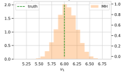
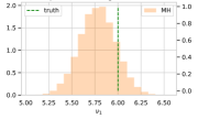
Interaction

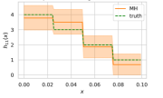
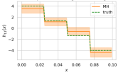
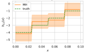
Figure 24: Posterior distribution on $f=(\nu_{1},h_{11})$ obtained with the MH sampler in the sigmoid model, in the three scenarios of Simulation 1 ($K=1$). The three columns correspond to the Excitation only (left), Mixed effect (center), and Inhibition only (right) scenarios. The first row contains the marginal distribution on the background rate $\nu_{1}$, and the second row represents the posterior mean (solid orange line) and 95% credible sets (orange areas) on the (self) interaction function $h_{11}$. The true parameter $f_{0}$ is plotted in dotted green line.

Softplus Excitation Mixed Inhibition
Background

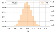
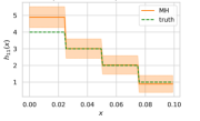
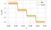
Figure 25: Posterior distribution on $f=(\nu_{1},h_{11})$ obtained with the MH sampler in the softplus model, in the three scenarios of Simulation 1 ($K=1$). The three columns correspond to the Excitation only (left), Mixed effect (center), and Inhibition only (right) scenarios. The first row contains the marginal distribution on the background rate $\nu_{1}$, and the second row represents the posterior mean (solid orange line) and 95% credible sets (orange areas) on the (self) interaction function $h_{11}$. The true parameter $f_{0}$ is plotted in dotted green line.

F.2 Simulation 3

This section contains our results regarding the estimated intensity function in the univariate and well-specified settings in Simulation 3 (see Figure 26), the estimated parameter in the mis-specified settings (see Figure 28), and the estimated interaction functions in the bivariate settings (see Figures 27 and 29).

(a) Excitation scenario

(b) Inhibition scenario

Figure 26: Intensity function on a subwindow of the observation window estimated via the variational posterior mean and via the posterior mean computed with the MH sampler, in the well-specified setting of Simulation 3 on $[0,10]$, using the fully-adaptive mean-field variational (FA-MF-VI) algorithm (Algorithm 2). The true intensity $\lambda_{t}^{1}(f_{0})$ is plotted in dotted green line.

$K=2$ Excitation
Background
                                                     Interaction functions

Figure 27: Posterior and model-selection variational posterior distributions on $f=(\nu,h)$ in the bivariate sigmoid model, well-specified setting, and Excitation setting of Simulation 3, evaluated by the non-adaptive MH sampler and the fully-adaptive mean-field variational (FA-MF-VI) algorithm (Algorithm 2). The first row contains the marginal distribution on the background rates $(\nu_{1},\nu_{2})$, and the second and third rows represent the (variational) posterior mean (solid line) and 95% credible sets (colored areas) on the four interaction function $h_{11},h_{12},h_{21},h_{22}$. The true parameter $f_{0}$ is plotted in dotted green line.

$K=1$ Mis-specified Excitation Inhibition
          Background
          Interaction

Figure 28: Model-selection variational posterior distributions on $f=(\nu_{1},h_{11})$ in the univariate sigmoid model and mis-specified setting of Simulation 3, evaluated by the fully-adaptive mean-field variational (FA-MF-VI) algorithm (Algorithm 2). The two columns correspond to a (mostly) Excitation (left) and a (mostly) Inhibition (right) settings. The first row contains the marginal distribution on the background rate $\nu_{1}$, and the second row represents the variational posterior mean (solid line) and 95% credible sets (colored areas) on the (self) interaction function $h_{11}$. The true parameter $f_{0}$ is plotted in dotted green line.

$K=2$ Inhibition
Background
                                                     Interaction functions

Figure 29: Posterior and model-selection variational posterior distributions on $f=(\nu,h)$ in the bivariate sigmoid model, well-specified setting, and Inhibition setting of Simulation 3, evaluated by the non-adaptive MH sampler and the fully-adaptive mean-field variational (FA-MF-VI) algorithm (Algorithm 2). The first row contains the marginal distribution on the background rates $(\nu_{1},\nu_{2})$, and the second and third rows represent the (variational) posterior mean (solid line) and 95% credible sets (colored areas) on the four interaction function $h_{11},h_{12},h_{21},h_{22}$. The true parameter $f_{0}$ is plotted in dotted green line.

F.3 Simulation 4

This section contains our results for the Inhibition setting of Simulation 4, i.e., the estimated graphs in (Figures 30 and 31), the heatmaps of the risk on the interaction functions in Figure 32, the estimated $L_{1}$-norms after the first step of Algorithm 3 in Figure 33, and the variational posterior distribution on the subset of the parameter in Figure 34.

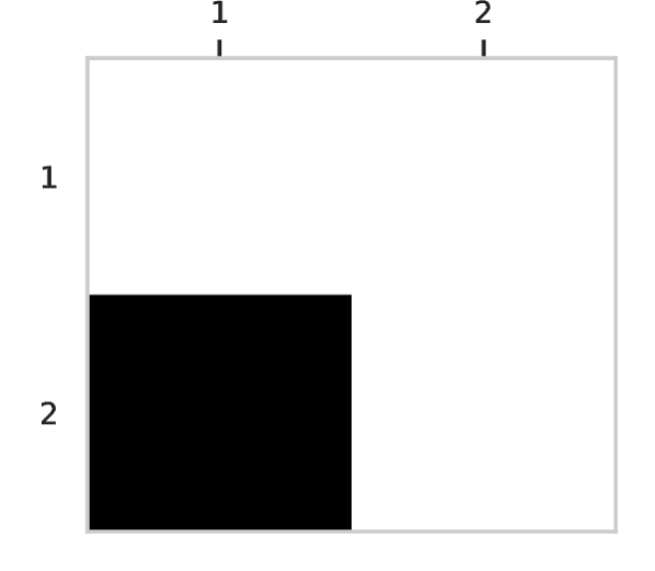
(a) $K=2$

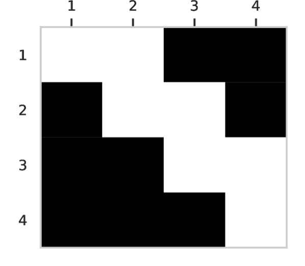
(b) $K=4$

(c) $K=8$

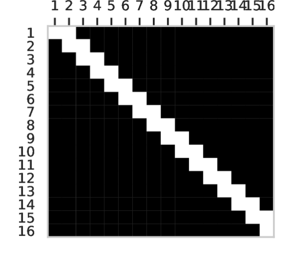
(d) $K=10$

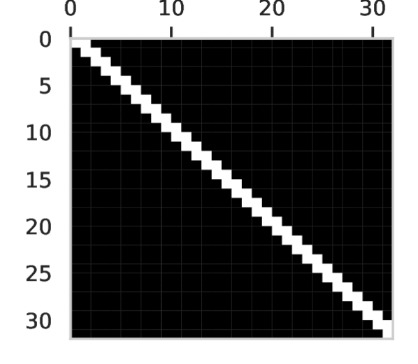
(e) $K=16$

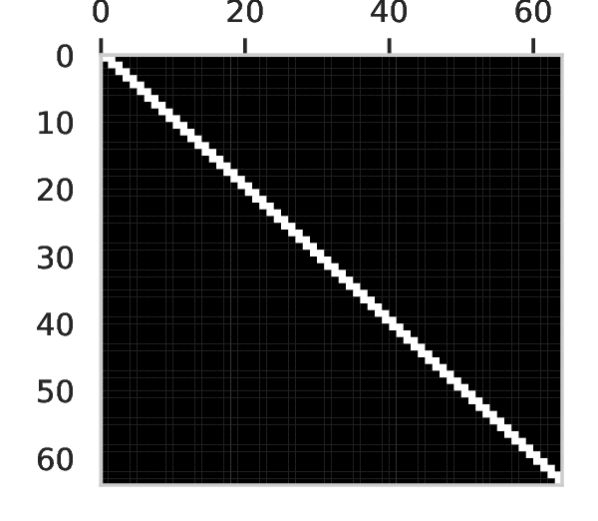
(f) $K=32$

Figure 30: Estimated graph parameter $\hat{\delta}$ (black=0, white=1) for $K=2,4,8,16,32,64$ in the Excitation scenario of Simulation 4.

(a) $K=2$

(b) $K=4$

(c) $K=8$

(d) $K=16$

(e) $K=32$

(f) $K=64$

Figure 31: Estimated graph parameter $\hat{\delta}$ (black=0, white=1) for $K=2,4,8,16,32,64$ in the Inhibition scenario of Simulation 4.

Function norms
Inhibition Ground-truth Error
$K=2$
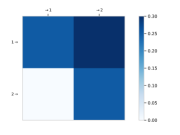
$K=4$
$K=8$
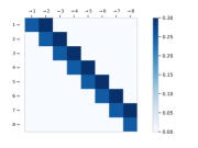
$K=16$
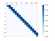
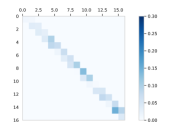
$K=32$
$K=64$

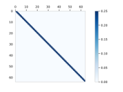
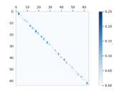
Figure 32: Heatmaps of the $L_{1}$-norms of the true parameter $h_{0}$, i.e., the entries of the matrix $S_{0}=(S^{0}_{lk})_{l,k}=(\left\lVert h_{lk}^{0}\right\rVert_{1})_{l,k}$ (left column) and $L_{1}$-risk, i.e., $(\varmathbb{E}^{Q}[\left\lVert h_{lk}^{0}-h_{lk}\right\rVert_{1}])_{l,k}$ (right column) after the first step of Algorithm 3, in the Inhibition scenario of Simulation 4. The rows correspond to $K=2,4,8,16,32,64$.

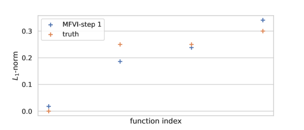
(a) $K=2$

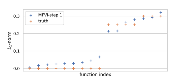
(b) $K=4$

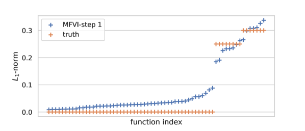
(c) $K=8$

(d) $K=16$

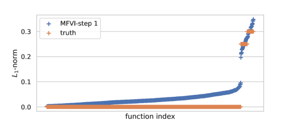
(e) $K=32$

(f) $K=64$

Figure 33: Estimated $L_{1}$-norms after the first step of Algorithm 3 (in blue), and ground-truth norms (in orange), plotted in increasing order, in the Inhibition scenario of Simulation 4, for the models with $K\in\{2,4,8,16,32,64\}$.

Inhibition Background $\nu_{1}$ Interaction functions $h_{11}$ and $h_{21}$

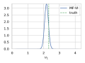
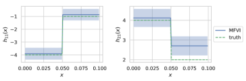
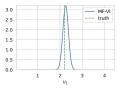
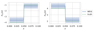
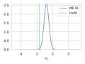
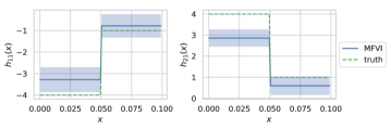
Figure 34: Model-selection variational posterior distributions on $\nu_{1}$ (left column) and interaction functions $h_{11}$ and $h_{21}$ (second and third columns) in the Inhibition scenario and multivariate sigmoid models of Simulation 4, computed with our two-step mean-field variational (MF-VI) algorithm (Algorithm 3). The different rows correspond to different multivariate settings $K=2,4,8,16,32,64$.

F.4 Simulation 5

In this section, we report some characteristics of the simulated data in Simulation 5, in particular the number of points and excursions in each setting (see Table 10). Moreover, we report the plots of the posterior distribution in a subset of the parameter in Figure 35.

Scenario	T	# events	# excursions	# local excursions
Excitation	50	2621	36	114
	200	10,729	155	473
	400	21,727	303	957
	800	42,904	596	1921
Inhibition	50	1747	49	134
	200	7019	222	529
	400	13,819	466	1053
	800	27,723	926	2118

Table 10: Number of points and global and average local excursions in the multidimensional data sets of Simulation 5 ($K=10$).

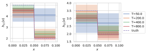
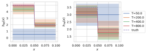
(a) Excitation scenario

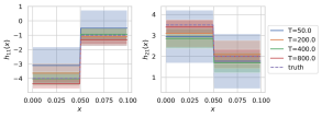
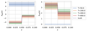
(b) Inhibition scenario

Figure 35: Model-selection variational posterior on two interaction functions $h_{66}$ and $h_{76}$, for different observation lengths $T\in\{50,200,400,800\}$, in the Excitation and Inhibition scenarios in Simulation 5 with $K=10$. We note that in this simulation, the true number of basis functions is 2 and is well recovered for all values of $T$. The estimation of these two interaction functions is poor for the smallest $T$, however, it improves when $T$ increases.

F.5 Simulation 6

This section contains the estimated graphs (Figures 36 and 38), the variational posterior distribution on a subset of the parameter (Figures 37 and 39), in the mis-specified settings of Simulation 6.

(a) Excitation scenario

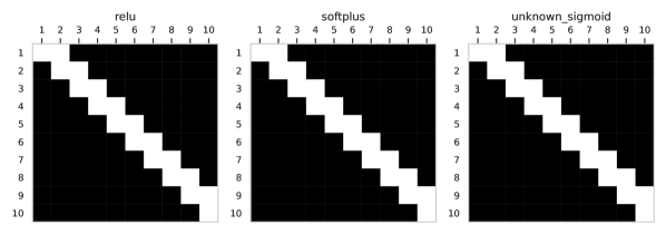
(b) Inhibition scenario

Figure 36: Estimated graph after thresholding the $L_{1}$-norms using the “gap” or “slope change” heuristic, in the different settings of mis-specified link functions of Simulation 6, and in the Excitation and Inhibition scenarios. We observe that the true graph (with non-null principal and first off-diagonal) is correctly estimated for the ReLU mis-specification setting, while some errors happen in the two other link settings, in particular in the Inhibition scenario.

(a) Excitation scenario

(b) Inhibition scenario

Figure 37: Estimated interaction functions $h_{66}$ and $h_{76}$ in the mis-specified settings of Simulation 6, where the data is generated from a Hawkes model with ReLU, softplus, or a mis-specified link function, and in the Excitation and Inhibition scenarios. We note that the estimation of the interaction functions is deteriorated in these mis-specified cases, however the sign of the functions are still recovered.

(a) Excitation scenario

(b) Inhibition scenario

Figure 38: Estimated graph after thresholding the $L_{1}$-norms, when using Algorithm 3 with different support upper bounds $A^{\prime}\in\{0.5,0.1,0.2,0.4\}$, containing the true memory parameter $A=0.1$, in the settings of Simulation 7. We note that the true graph (with non-null principal and first off-diagonal) is correctly estimated in all cases, in the Excitation scenario (first row) and in the Inhibition scenario (second row).

(a) Excitation scenario

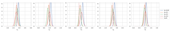
(b) Inhibition scenario

Figure 39: Estimated background rates $\nu_{k}$ for $k=1,\dots,5$ when using different values of the upper bound parameter $A\in\{0.05,0.1,0.2,0.4\}$, in the two scenarios of Simulation 8. As expected, the background rates are better estimated in the well-specified setting $A=A_{0}=0.1$; nonetheless, when $A$ is not too far above $A_{0}$, the estimation does not deteriorate too much, in particular in the Inhibition scenarios.

References

- Adams et al. (2009) Ryan Prescott Adams, Iain Murray, and David J. C. MacKay. Tractable nonparametric bayesian inference in poisson processes with gaussian process intensities. In Proceedings of the 26th Annual International Conference on Machine Learning, ICML ’09, page 9–16, New York, NY, USA, 2009. Association for Computing Machinery. ISBN 9781605585161. doi: 10.1145/1553374.1553376. URL https://doi.org/10.1145/1553374.1553376.
- Arbel et al. (2013) J. Arbel, G. Gayraud, and J. Rousseau. Bayesian adaptive optimal estimation using a sieve prior. Scand. J. Statist., 40:549–570, 2013.
- Bacry and Muzy (2015) Emmanuel Bacry and Jean-Francois Muzy. Second order statistics characterization of hawkes processes and non-parametric estimation, 2015.
- Bacry et al. (2020) Emmanuel Bacry, Martin Bompaire, Stéphane Gaïffas, and Jean-Francois Muzy. Sparse and low-rank multivariate hawkes processes. Journal of Machine Learning Research, 21(50):1–32, 2020.
- Bishop (2006) Christopher M. Bishop. Pattern recognition and machine learning. Information Science and Statistics. Springer, New York, 2006. ISBN 978-0387-31073-2; 0-387-31073-8. doi: 10.1007/978-0-387-45528-0. URL https://doi-org.proxy.bu.dauphine.fr/10.1007/978-0-387-45528-0.
- Bonnet et al. (2021) Anna Bonnet, Miguel Martinez Herrera, and Maxime Sangnier. Maximum likelihood estimation for hawkes processes with self-excitation or inhibition. Statistics & Probability Letters, 179:109214, 2021.
- Bremaud and Massoulie (1996) Pierre Bremaud and Laurent Massoulie. Stability of nonlinear hawkes processes. The Annals of Probability, 1996.
- Cai et al. (2021) Biao Cai, Jingfei Zhang, and Yongtao Guan. Latent network structure learning from high dimensional multivariate point processes, 2021.
- Carmona and Nicholls (2022) Chris U. Carmona and Geoff K. Nicholls. Scalable semi-modular inference with variational meta-posteriors, 2022. URL https://arxiv.org/abs/2204.00296.
- Carstensen et al. (2010) Lisbeth Carstensen, Albin Sandelin, Ole Winther, and Niels R Hansen. Multivariate hawkes process models of the occurrence of regulatory elements. BMC bioinformatics, 11(1):1–19, 2010.
- Chen et al. (2017a) Shizhe Chen, Ali Shojaie, Eric Shea-Brown, and Daniela Witten. The multivariate hawkes process in high dimensions: Beyond mutual excitation. arXiv:1707.04928v2, 2017a.
- Chen et al. (2017b) Shizhe Chen, Daniela Witten, and Ali Shojaie. Nearly assumptionless screening for the mutually-exciting multivariate Hawkes process. Electron. J. Stat., 11(1):1207–1234, 2017b. ISSN 1935-7524. doi: 10.1214/17-EJS1251. URL https://doi.org/10.1214/17-EJS1251.
- Costa et al. (2020) Manon Costa, Carl Graham, Laurence Marsalle, and Viet Chi Tran. Renewal in hawkes processes with self-excitation and inhibition. Advances in Applied Probability, 52(3):879–915, 2020. doi: 10.1017/apr.2020.19.
- Daley and Vere-Jones (2007) Daryl J Daley and David Vere-Jones. An introduction to the theory of point processes: volume II: general theory and structure. Springer Science & Business Media, 2007.
- Deutsch and Ross (2022) Isabella Deutsch and Gordon J. Ross. Bayesian estimation of multivariate hawkes processes with inhibition and sparsity, 2022. URL https://arxiv.org/abs/2201.05009.
- Donner and Opper (2019) Christian Donner and Manfred Opper. Efficient bayesian inference of sigmoidal gaussian cox processes, 2019.
- Donnet et al. (2020) Sophie Donnet, Vincent Rivoirard, and Judith Rousseau. Nonparametric Bayesian estimation for multivariate Hawkes processes. Ann. Statist., 48(5):2698–2727, 2020. ISSN 0090-5364. doi: 10.1214/19-AOS1903. URL https://doi-org.proxy.bu.dauphine.fr/10.1214/19-AOS1903.
- Eichler et al. (2017) Michael Eichler, Rainer Dahlhaus, and Johannes Dueck. Graphical modeling for multivariate hawkes processes with nonparametric link functions. Journal of Time Series Analysis, 38(2):225–242, 2017.
- Gerhard et al. (2017) Felipe Gerhard, Moritz Deger, and Wilson Truccolo. On the stability and dynamics of stochastic spiking neuron models: Nonlinear hawkes process and point process glms. PLOS Computational Biology, 13:1–31, 02 2017. doi: 10.1371/journal.pcbi.1005390. URL https://doi.org/10.1371/journal.pcbi.1005390.
- Golub and Welsch (1969) Gene H Golub and John H Welsch. Calculation of gauss quadrature rules. Mathematics of computation, 23(106):221–230, 1969.
- Hansen et al. (2015) Niels Richard Hansen, Patricia Reynaud-Bouret, and Vincent Rivoirard. Lasso and probabilistic inequalities for multivariate point processes. Bernoulli, 21(1):83–143, 2015. ISSN 1350-7265. doi: 10.3150/13-BEJ562. URL http://dx.doi.org/10.3150/13-BEJ562.
- Hawkes (1971) Alan G Hawkes. Point spectra of some mutually exciting point processes. Journal of the Royal Statistical Society: Series B (Methodological), 33(3):438–443, 1971.
- Hawkes (2018) Alan G. Hawkes. Hawkes processes and their applications to finance: a review. Quantitative Finance, 18(2):193–198, 2018. doi: 10.1080/14697688.2017.1403131. URL https://doi.org/10.1080/14697688.2017.1403131.
- Kingman (1993) J. F. C. Kingman. Poisson processes, volume 3 of Oxford Studies in Probability. The Clarendon Press Oxford University Press, New York, 1993. ISBN 0-19-853693-3. Oxford Science Publications.
- Lemonnier and Vayatis (2014) Remi Lemonnier and Nicolas Vayatis. Nonparametric markovian learning of triggering kernels for mutually exciting and mutually inhibiting multivariate hawkes processes. In Joint European Conference on Machine Learning and Knowledge Discovery in Databases, pages 161–176. Springer, 2014.
- Lu and Abergel (2018) Xiaofei Lu and Frédéric Abergel. High-dimensional hawkes processes for limit order books: modelling, empirical analysis and numerical calibration. Quantitative Finance, 18(2):249–264, 2018.
- Malem-Shinitski et al. (2021) Noa Malem-Shinitski, Cesar Ojeda, and Manfred Opper. Nonlinear hawkes process with gaussian process self effects, 2021.
- Mei and Eisner (2017) Hongyuan Mei and Jason Eisner. The neural hawkes process: A neurally self-modulating multivariate point process, 2017.
- Mohler et al. (2011) G. O. Mohler, M. B. Short, P. J. Brantingham, F. P. Schoenberg, and G. E. Tita. Self-exciting point process modeling of crime. Journal of the American Statistical Association, 106(493):100–108, 2011. doi: 10.1198/jasa.2011.ap09546. URL https://doi.org/10.1198/jasa.2011.ap09546.
- Nieman et al. (2021) Dennis Nieman, Botond Szabo, and Harry van Zanten. Contraction rates for sparse variational approximations in gaussian process regression, 2021. URL https://arxiv.org/abs/2109.10755.
- Ogata (1999) Yosihiko Ogata. Seismicity analysis through point-process modeling: A review. Seismicity patterns, their statistical significance and physical meaning, pages 471–507, 1999.
- Ohn and Lin (2021) Ilsang Ohn and Lizhen Lin. Adaptive variational bayes: Optimality, computation and applications, 2021.
- Olinde and Short (2020) Jack Olinde and Martin B. Short. A self-limiting hawkes process: Interpretation, estimation, and use in crime modeling. In 2020 IEEE International Conference on Big Data (Big Data), pages 3212–3219, 2020. doi: 10.1109/BigData50022.2020.9378017.
- Pfaffelhuber et al. (2022) Peter Pfaffelhuber, Stefan Rotter, and Jakob Stiefel. Mean-field limits for non-linear hawkes processes with excitation and inhibition. Stochastic Processes and their Applications, 2022.
- Polson et al. (2012) Nicholas G. Polson, James G. Scott, and Jesse Windle. Bayesian inference for logistic models using polya-gamma latent variables, 2012. URL https://arxiv.org/abs/1205.0310.
- Ray and Szabó (2021) Kolyan Ray and Botond Szabó . Variational bayes for high-dimensional linear regression with sparse priors. Journal of the American Statistical Association, pages 1–12, jan 2021. doi: 10.1080/01621459.2020.1847121. URL https://doi.org/10.1080.
- Shen and Ghosal (2015) Weining Shen and Subhashis Ghosal. Adaptive bayesian procedures using random series priors. Scandinavian Journal of Statistics, 42(4):1194–1213, 2015. doi: https://doi.org/10.1111/sjos.12159. URL https://onlinelibrary.wiley.com/doi/abs/10.1111/sjos.12159.
- Sulem et al. (2021) Deborah Sulem, Vincent Rivoirard, and Judith Rousseau. Bayesian estimation of nonlinear hawkes process, 2021.
- Titsias and Lázaro-Gredilla (2011) Michalis Titsias and Miguel Lázaro-Gredilla. Spike and slab variational inference for multi-task and multiple kernel learning. In J. Shawe-Taylor, R. Zemel, P. Bartlett, F. Pereira, and K.Q. Weinberger, editors, Advances in Neural Information Processing Systems, volume 24. Curran Associates, Inc., 2011. URL https://proceedings.neurips.cc/paper/2011/file/b495ce63ede0f4efc9eec62cb947c162-Paper.pdf.
- van der Vaart and van Zanten (2009a) A. W. van der Vaart and J. H. van Zanten. Adaptive bayesian estimation using a gaussian random field with inverse gamma bandwidth. The Annals of Statistics, 37(5B), oct 2009a. doi: 10.1214/08-aos678. URL https://doi.org/10.1214.
- van der Vaart and van Zanten (2009b) A. W. van der Vaart and J. H. van Zanten. Adaptive Bayesian estimation using a Gaussian random field with inverse gamma bandwidth. Ann. Statist., 37(5B):2655–2675, 2009b. ISSN 0090-5364. doi: 10.1214/08-AOS678. URL https://doi-org.proxy.bu.dauphine.fr/10.1214/08-AOS678.
- Wang et al. (2016) Yichen Wang, Bo Xie, Nan Du, and Le Song. Isotonic hawkes processes. In Proceedings of the 33rd International Conference on International Conference on Machine Learning - Volume 48, ICML’16, page 2226–2234. JMLR.org, 2016.
- Zhang and Gao (2020) Fengshuo Zhang and Chao Gao. Convergence rates of variational posterior distributions. The Annals of Statistics, 48(4):2180 – 2207, 2020.
- Zhang et al. (2020) Rui Zhang, Christian Walder, and Marian-Andrei Rizoiu. Variational inference for sparse gaussian process modulated hawkes process. Proceedings of the AAAI Conference on Artificial Intelligence, 34(04):6803–6810, Apr 2020. ISSN 2159-5399. doi: 10.1609/aaai.v34i04.6160. URL http://dx.doi.org/10.1609/aaai.v34i04.6160.
- Zhou et al. (2020) Feng Zhou, Zhidong Li, Xuhui Fan, Yang Wang, Arcot Sowmya, and Fang Chen. Efficient inference for nonparametric hawkes processes using auxiliary latent variables. Journal of Machine Learning Research, 21(241):1–31, 2020. URL http://jmlr.org/papers/v21/19-930.html.
- Zhou et al. (2021a) Feng Zhou, Quyu Kong, Yixuan Zhang, Cheng Feng, and Jun Zhu. Nonlinear hawkes processes in time-varying system, 2021a.
- Zhou et al. (2021b) Feng Zhou, Yixuan Zhang, and Jun Zhu. Efficient inference of flexible interaction in spiking-neuron networks, 2021b.
- Zhou et al. (2022) Feng Zhou, Quyu Kong, Zhijie Deng, Jichao Kan, Yixuan Zhang, Cheng Feng, and Jun Zhu. Efficient inference for dynamic flexible interactions of neural populations. Journal of Machine Learning Research, 23(211):1–49, 2022. URL http://jmlr.org/papers/v23/21-1273.html.