Economics of NFTs: The Value of Creator Royalties

Abstract

Non-Fungible Tokens (NFTs) promise to revolutionize how content creators (e.g., artists) price and sell their work. One core feature of NFTs is the option to embed creator royalties which earmark a percentage of future sale proceeds to creators, each time their NFTs change hands. As popular as this feature is in practice, its utility is often questioned because buyers, the argument goes, simply “price it in at the time of purchase”. As intuitive as this argument sounds, it is incomplete. We find royalties can add value to creators in at least three distinct ways. (i) Risk sharing: when creators and buyers are risk sensitive, royalties can improve trade by splitting the risks associated with future price volatility; (ii) Dynamic pricing: in the presence of information asymmetry, royalties can extract more revenues from better-informed speculators over time, mimicking the benefits of “dynamic pricing”; (iii) Price discrimination: when creators sell multi-unit NFT collections, royalties can better capture value from heterogeneous buyers. Our results suggest creator royalties play an important and sometimes overlooked role in the economics of NFTs.

Keywords: Blockchain, Cryptocurrency, Non-Fungible Tokens, NFTs, Creator Royalties, Information Asymmetry, Risk Aversion, Price Discrimination.

1 Introduction

Non-Fungible Tokens (NFTs) are cryptographic assets that can exist on a blockchain alongside cryptocurrencies like Bitcoin. But while cryptocurrencies are fungible, NFTs are not, that is, they are often tied to unique, non-interchangeable assets. As such, they are considered an ideal vehicle to represent ownership of a variety of different types of unique assets, including digital and physical art, identities, property rights, etc. A total of $25B worth of NFTs were traded in the first three quarters of 2022 (NonFungible.com 2022). One notable example is the CryptoPunk collection, a digital representation of punk-culture-inspired figures on Ethereum’s blockchain. A single image, Punk 4464, was sold for a record high $2.6M in July 2022.

One central feature of NFTs is that they allow creators to embed royalties (Kent 2021). These are usually set as a percentage of the sale price that is transferred to the creator in future (re)sales. To date, over $1.8B in royalties have been paid to creators on the Ethereum blockchain (Qadir & Parker 2022), and for many creators, royalty revenues have dwarfed revenues from the initial sale (NFTStatistics.eth 2022).

Despite these documented benefits, there is an ongoing debate regarding the long-term added value and viability of creator royalties. Critics argue that rational buyers simply price in the cost of royalties at the time of purchase. For example, if a creator sets a royalty rate of 10%, buyers will only pay 90% of the expected future value of the work, and creators will not gain any more (in expectation) than if they had set royalties to zero. What, then, is their purpose?

In the current state of affairs, NFT exchanges play a critical role in guiding the market to an equilibrium state of acceptance or rejection of royalty features. This is because creator royalties are not enforced at the smart contract level. Royalty standards, like EIP-2981 (Burks et al. 2020), do not actually handle royalty payments. Instead, they provide a standard method by which NFTs can request royalty payments. It thus remains at the discretion of individual exchanges (or the buyer and seller themselves) whether the requested royalties are enforced and paid.

Some NFT marketplaces have found the aforementioned criticisms so compelling, that they have started removing the enforcement of NFT royalty payments altogether (Hayward 2022a). Others have openly re-affirmed their commitment to maintaining and improving creator royalties. Quoting, for instance, a November 6, 2022 tweet by OpenSea, one of the largest NFT marketplaces:

“There’s been a lot of discussion over the past few months about business models for NFT creators & whether creator fees (“royalties”) are viable. Given our role in the ecosystem, we want to take a thoughtful, principled approach to this topic & to lead w/ solutions.”

Do royalties add value for creators, or can they be safely discontinued with little consequence? This paper seeks to shed some light on the ongoing debate.

Model Outline

We develop a relatively simple model of NFT sales where a creator (seller) mints an NFT tied to an asset. The creator chooses a fixed mint price and has the option of attaching a (percentage) royalty. For royalties to not be trivially ruled out, we require at least a two-period model, where there is a possibility that a future trade can trigger the royalty payment. As is the case in most NFT markets, strategic speculators (which in practice are sometimes automated bots running algorithms) are present, and seek to purchase NFTs from the creator before anyone else, with the hope of reselling them at a later date to end-buyers, if prices appreciate. They are strategic in the sense that they can fully price in the cost of royalties. End-buyer valuations are usually uncertain at the initial sale and purchase time, and this creates potential future upside but also downside risk for both creators and speculators. We study three distinct situations where NFTs have the potential to add value: (i) when agents are risk averse; (ii) when speculators are better informed about the market prospects of the NFT; (iii) when creators have multiple NFTs to sell as part of a collection, to multiple buyers with heterogeneous valuations.

Main Results

We find that as intuitive as the aforementioned criticism sounds, it is incomplete. In a bare-bones benchmark model of an NFT sale, the intuition does indeed hold. Royalties are rendered useless as rational buyers price their cost in at the time of purchase. But this result reverses in all three aforementioned situations. More specifically, creator royalties can unlock the following benefits:

Risk-Sharing (under risk aversion): In Section 4, we show that when creators and speculators are risk-sensitive, royalties allow both agents to split the risk of future price volatility. This can increase creator utility and improve the chances of a successful transaction (facilitate trade).

Dynamic pricing (under information asymmetry): In Section 5, we show that in the presence of speculators that are better-informed about the NFT market, royalties allow creators to piggy-back off of this information, and retain some upside in case of future price appreciation. Put differently, royalties can be used to mimic the benefits of “dynamic pricing”, even as NFT mint prices remain static.

Price discrimination (in multi-unit collections): In many instances, creators mint a collection of similar (or identical) NFTs all at once, and price them low, or even give them out for free. We study this setting in Section 6. These collection sales often generate a lot of buzz for the creators, and are sometimes so popular that they can overwhelm the underlying blockchain (Geron 2022, Nelson 2022). Here, royalties allow creators to better extract value from buyers with heterogeneous valuations for the various items of the collection. The effect, in this case, is not driven by risk aversion, or information asymmetry, but rather by the mere fact that buyers have heterogeneous valuations (e.g., different people can have different utilities for a piece of art), which opens the door to price discrimination. Importantly, the above benefits of royalties persist, even as fully rational buyers price their cost in at the time of purchase.

Note, our models of information asymmetry (Section 5) and collection pricing (Section 6) predict solutions where the creator gives the NFTs away for free, and obtains all their revenues from royalties. As mentioned, this type of outcome is observed in practice. Several high-profile NFT projects have adopted this strategy, for example Loot (Hayward 2022b), Art Gobblers (Carreras 2022) and GoblinTown distributed their collections for free, but set nonzero royalty rates (Loot requests 5%, Art Gobblers requests 6.9% and GoblinTown requests 7.5% royalties on OpenSea).

Many other projects, like the hugely successful Bored Ape Yacht Club, did not distribute their tokens for free, but instead sold their tokens for a nominal fee. Nevertheless, the creator, Yuga Labs, has made orders of magnitude more from royalty revenue than the initial sale (NFTStatistics.eth 2022). Yuga labs’ later projects, like the Bored Ape Kennel Club, gave the tokens away for free, and relied exclusively on royalties for their revenue. This is consistent with our models, which show that in many circumstances the creator can maximize profits by giving their tokens away for free and setting a positive royalty rate (Murray 2022).

Overall, our results suggest that the narrative that creator royalties serve no real purpose, is incomplete. Creator royalties can and do help creators in several different ways, even in the presence of fully rational buyers that price in their cost. As such, this feature plays an important and sometimes overlooked role in the economics of NFTs.

Related Work

Several prior works have studied the NFT markets empirically. Vasan et al. (2022) analyzed all sales of NFTs on the Foundation marketplace, but did not analyze royalties. Nadini et al. (2021) categorized different types of NFTs (e.g. “art,” “collectible,” “game” etc.) and mapped networks of traders and collections, but did not consider royalty payments. Ante (2021) analyzes the relationship between NFT sales and the price of Bitcoin and Ether.

Kireyev (2022) uses the CryptoPunks marketplace as a backdrop to study how the cost of bidding affects sales. CryptoPunks do not include creator royalties, and this analysis does not include royalty information in their theoretical model or empirical data.

NFT royalty payments have been measured empirically NFTStatistics.eth (2022), Qadir & Parker (2022), but existing works do not model royalty payments.

Several works have discussed the potential value of creator royalties (van Haaften-Schick & Whitaker 2022, Whitaker & Kräussl 2020) without explicitly modeling royalty payments.

Lovo & Spaenjers (2018) models art trading by a sequence of English auctions, but does not include royalty payments.

Other works (Su 2010, Cachon & Swinney 2009) have developed models for selling in the presence of strategic speculation, but they do not consider royalty payments.

The legal aspects of collecting royalty payment are discussed in Murray (2022).

More broadly, our work has implications for the literature studying the economics of token systems.

2 General Model

In this section, we describe our general model of NFT sales that underpins the specialized models in subsequent sections. There are three periods and three types of agents.

At time 0, a “creator” produces an item (or multiple items) that she wishes to sell by minting a corresponding NFT. Production and minting costs are denoted $c\geq 0$. She sets her fixed NFT mint price, $p_{0}\geq 0$, and possibly a royalty rate $r\in[0,1]$ which entitles her to receive (in addition to $p_{0}$) an $r$-fraction of future sales proceeds, if any.

At time $1$, a speculator can choose to purchase the NFT at $p_{0}$. He does so only if he expects to be able to resell it later and break even with respect to his outside option, which without loss of generality, we set to zero to simplify the exposition. If trade does not occur, the speculator exits the market.

At time $2$, an end-buyer appears who is willing to purchase the NFT at a stochastic valuation, $V$, with mean $\mu$, standard deviation $\sigma$, PDF $f$, and CDF $F$ (discrete distributions are also admissible). The distribution of $V$ is known to both creator and speculator at time 0, however, the speculator can add value to the trade in the following sense: If he owns the NFT at time 2, he does not have to commit to selling it at the creator’s mint price $p_{0}$. Instead, can sell it at the realization of $V$. In this case, a percentage $r$ of the sales proceeds is remitted to the creator. Conversely, if the speculator has exited prior to time $2$, the creator can try to sell the item to the buyer at the fixed mint price $p_{0}$ set at time 0. In this case, trade occurs only if the realization of $V\geq p_{0}$. This setup is meant to capture the dominant model of NFT sales in practice, where creators usually sell their NFTs at a fixed mint price, whereas resellers (speculators) operate primarily in the NFT aftermarket searching for the best returns. One technical note is that we assume throughout the paper if speculators are indifferent (from a utility perspective) between buying NFTs and not buying them, they always prefer to buy the most NFTs they can.

Using this model as a base, we consider three specializations:

Risk Aversion: In Section 4, we consider a situation where both the creator and the speculator are risk averse, specifically the creator and the speculator have a mean-variance utility.

Information asymmetry: In Section 5, we consider the situation where the speculator can be better informed regarding the future value of the NFT. Specifically, he learns the realization of $V$ before he needs to make a decision on purchasing the NFT at time $1$. This now gives the speculator an informational advantage over the creator, who only knows the distribution of $V$ at the time she chooses $p_{0}$.

Buyer Heterogeneity: In Sections 4 and 5, we assume the creator has a single NFT to sell. In Section 6, we consider the situation where the creator has more than one NFT to sell to more than one potential buyer.

3 When are Royalties Not Needed?

In this section, we analyze the significance of royalties in the bare-bones model which will serve as a benchmark, setting aside risk aversion, information asymmetry, and collections. Our focus here is on understanding three things: (i) what does trade look like when the creator is directly selling to the end-buyer? (ii) under what conditions can speculators add value as middle-men between creator and end-buyer? (iii) when are royalties NOT needed?

3.1 Direct Trade with an End-Buyer (No Speculator Present)

For now, consider the speculator is absent entirely and hence time 1 has no actions. By default, this implies royalties cannot play a role here (as mentioned, one requires at least two periods of trade to not trivially rule them out). Instead, the creator mints a NFT at time 0, hoping to sell it directly to an end-buyer with random valuation $V$ at time 2.

As discussed, the creator has to set the mint price $p_{0}$ before the realization of $V$ is known. One important implication is that for many common distributions of $V$, the optimal mint price will not be $p_{0}^{*}=\operatorname{E}[V]$, and the creator will not able to fully extract end-buyer willingness-to-pay, $\operatorname{E}[V]$. To see this, note that if $p_{0}\leq V$, then the buyer buys the item, and the creator earns $p_{0}$. On the other hand, if $V<p_{0}$, there is no trade and the creator earns nothing. Let $\mathbbm{1}_{V\geq p_{0}}$ be the corresponding indicator function. The creator’s expected profits are given by $p_{0}\cdot\operatorname{E}[\mathbbm{1}_{V\geq p_{0}}]-c$, which can be written as $p_{0}\cdot\Pr[V\geq p_{0}]-c.$ Her optimization problem can be written as

$$\max_{p_{0}}\quad p_{0}\cdot\Pr[V\geq p_{0}]-c.$$ (1)

Without loss of generality, we can ignore cost $c$ here (set to 0) to simplify exposition given it is merely an additive constant. For most common distributions, we have the following result:

Lemma 1.

When the creator is directly selling to an end-buyer, and assuming unimodality of the objective in (1), the optimal mint price, $p_{0}^{*}$, is given by the solution to the following first-order condition:

$$p_{0}f(p_{0})=1-F(p_{0}).$$ (2)

Depending on the distribution of $V$, the above may NOT have a closed-form solution. Even so, we can characterize the creator’s optimal profits without explicitly solving for the optimal mint price. By Markov’s inequality (aka, the first Chebyshev inequality), regardless of the distribution of $V$ and of the creator’s choice of $p_{0}$, the revenues satisfy

$$p_{0}\cdot\Pr[V\geq p_{0}]\leq\operatorname{E}[V],\quad\forall\ p_{0}\in[0,\infty),$$ (3)

with the inequality being strict whenever $V$ is “non-degenerate,” which we formally define below.

Definition 1.

A random variable, $V$, is called non-degenerate if $V$ is supported on at least two nonzero points, i.e., there exists points $0<v_{1}<v_{2}$ and a value $\epsilon$, with $0<\epsilon<(v_{2}-v_{1})/2$, such that $\Pr[v_{1}-\epsilon<V<v_{1}+\epsilon]>0$, and $\Pr[v_{2}-\epsilon<V<v_{2}+\epsilon]>0$.

For illustrative purposes, we outline a simple example below.

Example 1 (Markov’s Inequality at Work).

As an example, define the two-point distribution $V\sim v_{L}$ with prob. 1/2 and $v_{H}$ with prob. 1/2, where $0<v_{L}<v_{H}$. Then $\operatorname{E}[V]=\frac{v_{L}+v_{H}}{2}$, but $\max_{p_{0}}p_{0}\cdot\Pr[V\geq p_{0}]=\max\left(v_{L},\frac{v_{H}}{2}\right)$, which is strictly less than $\operatorname{E}[V]$, given $v_{L}>0$.

Price range	Best $p_{0}$	$\bf\Pr(V\geq p_{0})$	Creator E[Rev]	Speculator E[Rev]	End-Buyer E[Rev]
$p_{0}\leq v_{L}$	$v_{L}$	1	$v_{L}$	absent	$(v_{H}-v_{L})/2$
$v_{L}<p_{0}\leq v_{H}$	$v_{H}$	1/2	$v_{H}/2$	absent	0
$v_{H}<p_{0}$	indiff.	0	0	absent	0

Table 1: Creator and end-buyer revenues from Example 1 when the speculator is absent and without royalties.

To understand Example 1, consider the possible ranges for $p_{0}$ given in Table 1. If $p_{0}\leq v_{L}$, the probability of trade is 1 and the optimal $p_{0}=v_{L}$, which leads to expected revenues of $v_{L}\cdot 1$. If $p_{0}>v_{H}$, the probability of trade is 0 and there are no revenues to be made. And if $p_{0}$ is between $[v_{L},v_{H}]$, the probability of trade is 1/2. In the latter case, the optimal $p_{0}=v_{H}$ and expected revenues are $v_{H}\cdot 1/2$.

We formalize the main takeaway in the following corollary:

Corollary 1 (Absence of speculator).

In the absence of a speculator, and without the possibility of royalties, the creator’s optimal revenues are given by $\max_{p_{0}}p_{0}\Pr[V\geq p_{0}]$ and Markov’s inequality (3) implies she cannot fully extract expected end-buyer willingness-to-pay, $\operatorname{E}[V]$.

3.2 How Speculators can Improve Trade Outcomes (Absent Royalties)

Speculation is known to be rampant in NFT markets, and in this section we examine some of the implications of having a speculator present who can serve as a trade intermediary between creator and end-buyer. Royalties are still ruled out for the moment.

Suppose there exists a speculator arriving at time $1$, as described in the general model in Section 2. For the purposes of the benchmark model, the speculator and creator have the same information at the time the NFT purchasing decision needs to be made. However, the speculator has the advantage of operating in the aftermarket at time $2$, where he can sell the NFT to an end-buyer after observing the realization of $V$. This implies that the speculator, on average, is able to extract $\operatorname{E}[V]$ from the buyer. Denote the speculator’s sale price at time 2, $p_{2}$.

At time 0, the speculator is making his purchasing decision from the creator, anticipating that he can earn revenues amounting to $\operatorname{E}[V]$ from the end-buyer, at time 2. The speculator’s optimal strategy is to set his own price at time 2, to match the realization of $V$, $p_{2}=v$. Thus, Markov’s inequality is no longer relevant here.

In turn, the creator can set his own price at time 0 anticipating the speculator’s optimal strategy. In particular, the creator can set the mint price $p_{0}=\operatorname{E}[V]$, knowing that it is still rational for the speculator to purchase at this price (and break even with respect to his outside option). Compared to the previous Section 3.1, this can allow the creator to extract higher revenues, and also ensures that the creator will always prefer to sell to the speculator at time 0, rather than wait to sell to the end-buyer at time 2. The main takeaway is formalized in the corollary below.

Corollary 2 (Presence of an equally-informed speculator).

In the presence of an equally-informed speculator, without the possibility of royalties, the creator can “piggy-back” off the speculator’s access to the aftermarket to better capture end-buyer willingness-to-pay, obtaining excess profits (compared to the case without the speculator described in Corollary 1) of:

$$\Delta=\operatorname{E}[V]-\max_{p_{0}}\ \Big{(}p_{0}\cdot\Pr[V\geq p_{0}]\Big{)}>0.$$

The inequality is strict if $V$ is non-degenerate (Definition 1).

3.3 When are Royalties Not Needed?

As discussed, an intuitive argument often put forth in practice is that creator royalties don’t benefit the creator, because they will be “priced in” by buyers. Here, we extend the setting from the previous Section 3.2 to allow for royalties and show that when both creator and speculator are risk neutral (i.e., $\eta_{s}=\eta_{c}=0$) and have the same information sets, this argument is true! The creator obtains the same optimal revenue no matter what royalty rate she decides to set. Formally:

Theorem 1 (When are royalties NOT needed?).

When selling a single NFT, if both the creator and speculator have the same information and are risk neutral ($\eta_{s}=\eta_{c}=0$), then creator royalties play no effective role. In particular, any $\{p_{0}^{*},r^{*}\}$ satisfying $\{p_{0}^{*}=\mu(1-r^{*}),p_{0}^{*}\geq 0,r^{*}\in[0,1]\}$, maximize the creator’s expected profits, which are given by

$$\mu-c.$$

All proofs are provided in the appendix. Theorem 1 shows that creator royalties are effectively “priced in” in this type of setting, and do not confer any advantage to the creator.

Key Takeaways from Section 3

To summarize, there are two key takeaways from this benchmark section:

• Irrespective of royalties, the presence of speculators in the market can benefit creators, but only if they are equally informed;

• Royalties do NOT add value in the absence of risk aversion, information asymmetry or multi-item collections.

4 Royalties as a Risk-Sharing Mechanism

In this section, we expand the base model from Section 2 by assuming that the creator and speculator are sensitive to risk. This will reverse some of the previous findings.

Modifications to base model

Using the notation from Section 2, conditional on the speculator owning the NFT at time $2$ and selling it to the end-buyer, the agents’ profits at time 2 are given by:

$$v_{c}(p_{0},r) =p_{0}+rp_{2}-c\quad\mbox{(Creator profit)}$$

$$v_{s}(p_{0},r) =(1-r)p_{2}-p_{0}\quad\mbox{(Speculator profit).}$$

We consider a mean-variance utility over profits with risk parameters $\eta_{c}$ for the creator and $\eta_{s}$ for the speculator (alternative utility functions can be specified without affecting the qualitative results). Furthermore, as previously discussed, the speculator’s optimal strategy at time 2 is simply $p_{2}=v$, which extracts the maximum willingness-to-pay from the end-buyer, and ensures trade occurs; adding risk aversion does not alter this result given the speculator’s pricing decision is made after uncertainty realization. With this, agent utilities at time $0$ can be written as

$$u_{c}(p_{0},r) =\operatorname{E}[v_{c}(p_{0},r)]-\eta_{c}\operatorname{Var}[v_{c}(p_{0},r)]\quad\mbox{(Creator utility)}$$

$$u_{s}(p_{0},r) =\operatorname{E}[v_{s}(p_{0},r)]-\eta_{s}\operatorname{Var}[v_{s}(p_{0},r)]\quad\mbox{(Speculator utility),}$$

where $\operatorname{E}[v_{c}(p_{0},r)]=p_{0}+r\mu-c$, $\operatorname{E}[v_{s}(p_{0},r)]=(1-r)\mu-p_{0}$, $Var[v_{c}(p_{0},r)]=r^{2}\sigma^{2}$, $Var[v_{s}(p_{0},r)]=(1-r)^{2}\sigma^{2}$. With these definitions, the creator’s objective is to maximize $u_{c}$ by choosing the sale price, $p_{0}$, and creator royalty, $r$, subject to the speculator’s participation constraint at time $0$, $u_{s}\geq 0$. Formally:

$$\max_{p_{0},r} \quad\operatorname{E}\left[v_{c}(p_{0},r)\right]-\eta_{c}\operatorname{Var}[v_{c}(p_{0},r)]$$ (4)

$$\mbox{subject to:}\quad u_{s}(p_{0},r)\geq 0,$$ (5)

with $u_{s}(p_{0},r)=(1-r)\mu-p_{0}-\eta_{s}(1-r)^{2}\sigma^{2}$.

Analysis

The objective function in (4) can be written as

$$E\left[v_{s}\right]-\eta_{c}\operatorname{Var}_{s}[v_{s}]=p_{0}+r\mu-c-\eta_{c}r^{2}\sigma^{2}.$$

Given Equation 5 will bind, and re-arranging terms, the creator’s maximization problem can be rewritten as a quadratic program over $r$:

$$\max_{r}\quad p_{0}+r\mu-c-\eta_{c}r^{2}\sigma^{2}$$ (6)

$$\mbox{subject to:}\quad p_{0}=\mu(1-r)-\eta_{s}\sigma^{2}(1-r)^{2}.$$ (7)

Solution Without Royalties

If the option of royalties is removed entirely ($r=0$), as some exchanges are contemplating doing, then the creator’s optimization problem simplifies. From Equation 7, the price at which the speculator is willing to purchase the NFT is given by

$$p_{0,r=0}^{*}=\mu-\eta_{s}\sigma^{2}.$$

Replacing this in the objective in (6) while setting $r=0$, leads to a creator utility absent royalties given by:

$$u_{c,r=0}^{*}=\mu-c-\eta_{s}\sigma^{2}.$$ (8)

Solution With Royalties

The solution to (6) and (7) is provided in the following lemma.

Lemma 2.

Under risk aversion, the creator’s optimal NFT mint price, royalties and utility are given by

$$p_{0}^{*}=\frac{\eta_{c}}{(\eta_{c}+\eta_{s})^{2}}\Big{(}(\eta_{c}+\eta_{s})\mu-\eta_{c}\eta_{s}\sigma^{2}\Big{)},\quad r^{*}=\frac{\eta_{s}}{\eta_{s}+\eta_{c}},\quad u_{c}^{*}=\mu-c-\left(\frac{\eta_{c}\eta_{s}}{\eta_{c}+\eta_{s}}\right)\sigma^{2}.$$ (9)

Comparing creator utilities $u_{c}^{*}$ to $u_{c,r=0}^{*}$ brings us to the formal result:

Theorem 2 (Risk Aversion).

Under risk aversion, creator royalties increase creator utility by an amount

$$\Delta=\sigma^{2}\frac{\eta_{s}^{2}}{\eta_{s}+\eta_{c}}.$$

Further, $\Delta$ increases

• as future price uncertainty, $\sigma$, increases

• as the speculator becomes more risk averse (i.e., as $\eta_{s}$ increases)

• as the creator becomes less risk averse (i.e., as $\eta_{c}$ decreases)

As an illustrative example, assume the creator and speculator have the same risk aversion coefficient ($\eta_{s}=\eta_{c}$). In this case, the optimal royalty rate simplifies to $r^{*}=1/2$, and the utility gains generated by royalties (over the no-royalty model) simplify to $\sigma^{2}/2$, that is, the creator and speculator equally share exposure to future price volatility.

Royalties Expand Trade Under Risk Aversion

A closely related benefit of royalties is that they can increase the propensity of trade, that is, they expand the space of parameters in which trade occurs between creator and speculator. To see this, note that the results in Lemma 2 require the extra condition $u_{c}^{*}\geq 0$, otherwise there is no trade. Comparing $u_{c}^{*}\geq 0$ to $u_{c,r=0}^{*}\geq 0$, the former is easier to satisfy. As an example, let’s assume $\mu=1,\sigma=1,c=0,\eta_{s}=2,\eta_{c}=1$. Then the creator’s utility with royalties equals $1/3$, whereas her utility without royalties would be negative, and no trade would occur. More formally, let $\mathbbm{T}$ be the set of parameters for which trade would occur if royalties were allowed, but would not occur in their absence.

Corollary 3 (Royalties expand the trade region).

Under risk aversion, royalties increase the region of trade, that is, the set $\mathbbm{T}=\{\mu,c,\eta_{s},\eta_{c},\sigma\ |\ u_{c}^{*}\geq 0\ \cap u_{c,r=0}^{*}<0\ \mu\geq 0\ \cap 0\leq c\leq\mu\ \cap\eta_{s}\geq 0\ \cap\eta_{c}\geq 0\}$ is non-empty. A visual representation is provided in Figure 1.

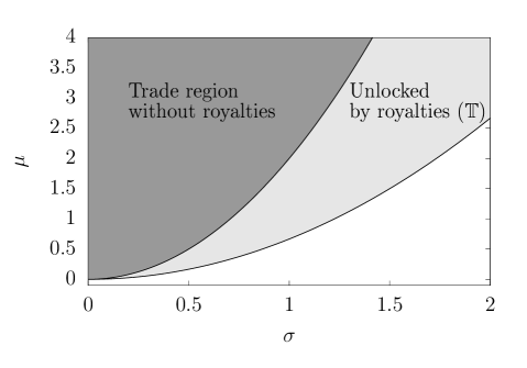
Figure 1: The region of trade unlocked by royalties under risk aversion, in $\{\mu,\sigma\}$ space ($\eta_{c}=1,\eta_{s}=2,c=0$).

Remark 1 (Robustness Check: Differing market views).

Our model of risk aversion assumes the creator and the speculator share the same outlook on future prices, i.e., $\operatorname{E}[V]=\mu$, and $\operatorname{Var}(V)=\sigma^{2}$. In Appendix C, we show that the qualitative results in this section still hold when the creator and the buyer have conflicting views about the distribution of $V$.

Key Takeaways from Section 4

To summarize, there are two key takeaways from this section that focuses on risk aversion:

• Royalties increase creator utility when speculators are risk averse

• Royalties serve as a risk-sharing mechanism that can improve trade outcomes.

5 Royalties as a Dynamic Pricing Mechanism

In this section, we expand the base model in Section 2 to include information asymmetry. In practice, speculators may be better-informed about the prospects of the aftermarket. To capture this, suppose the speculator has better information than the creator regarding customer willingness-to-pay. A simple way to model this advantage is to assume that the speculator can observe the realization of $V$ before deciding whether to purchase the NFT from the creator. Creators, in turn, are aware of their disadvantage.

5.1 Trade under Information Asymmetry (Without Royalties)

Suppose for the moment that royalties are not allowed. In this case, the speculator’s informational advantage collapses the outcome of the game for the creator, to that of Section 3.1, leaving her indifferent between selling to the speculator or to the end-buyer. To see this, consider that at time 0, if $p_{0}>v$, the speculator refuses trade, and if $p_{0}\leq v$, the speculator purchases the NFT, knowing that he can sell it for a profit $v-p_{0}\geq 0$ to the end-buyer.

There are two implications. First, the speculator effectively mimics the end-buyer, and front-runs him out of his expected profits. Second, the creator can no longer extract all the revenue from either the speculator or the end-buyer. In particular, the creator’s expected revenues collapse to those absent the speculator described in Corollary 1.

For convenience, we repeat here the creator’s optimization problem, which remains the same under this information asymmetry extension:

$$\max_{p_{0}}p_{0}\cdot\Pr[V>p_{0}],$$

and the previous result that the creator cannot extract maximum revenues, based on Markov’s inequality,

$$p_{0}\cdot\Pr[V\geq p_{0}]\leq\operatorname{E}[V],\quad\forall\ p_{0}\in[0,\infty).$$

It is useful to go through an illustrative example.

Example 2.

Suppose, as in Example 1, $V$ is either $v_{L}$ or $v_{H}$, each with probability 1/2, but now, a better-informed speculator is present. Agent expected revenues are given in Table 2 and an illustration of how the creator’s revenues vary with her choice of mint price $p_{0}$ are shown in Figure 2(a). As in Example 1, the creator’s optimal revenues are again given by $\max\{v_{L},v_{H}/2\}<E[V]$. But one difference here is that the speculator “front-runs” the end-buyer, and leaves him without any revenues.

Price range	Best $p_{0}$	$\bf\Pr(V\geq p_{0})$	Creator E[Rev]	Speculator E[Rev]	End-Buyer E[Rev]
$p_{0}\leq v_{L}$	$v_{L}$	1	$v_{L}$	$(v_{H}-v_{L})/2$	0
$v_{L}<p_{0}\leq v_{H}$	$v_{H}$	1/2	$v_{H}/2$	$0$	0
$v_{H}<p_{0}$	indiff.	0	0	0	0

Table 2: Agent revenues from Example 2 when the speculator has an informational advantage.

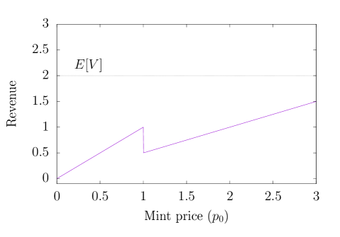
(a) Without Royalties

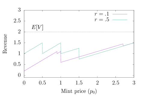
(b) With Royalties

Figure 2: Creator revenues from Example 2 (with $v_{L}=1,v_{H}=3$) as a function of mint price $p_{0}$. When the speculator is better-informed, the creator cannot extract the maximum expected revenue $E[V]=2$ without royalties.

The following corollary recaps the main points.

Corollary 4 (No Royalties, Better-Informed Speculator).

In the presence of a better-informed speculator, without the possibility of royalties, the creator’s expected profits collapse back to those of Corollary 1. The creator can no longer “piggy-back” off the speculator’s access to the aftermarket (described in Corollary 2).

5.2 The Impact of Royalties under Information Asymmetry

We now introduce royalties to the setup of Section 5.1, maintaining the speculator’s informational advantage. Both the modeling modifications required, and the analysis, are more involved here.

As before, at time 0, the creator sets her mint price $p_{0}$ and royalty rate, $r$. At time 1, the speculator learns the valuation, $v$, and will purchase the NFT if and only if $(1-r)v-p_{0}\geq 0$. If the speculator does purchase the NFT, the creator’s expected profits are given by $p_{0}+rE\left[V~{}\middle|~{}(1-r)V\geq p_{0}\right]$, where the second term represents the royalties paid back to the creator once the speculator re-sells the NFT to an end-customer at time 2. Notice that the expectation is now conditional. This scenario occurs with probability $\Pr[(1-r)V\geq p_{0}]$. On the other hand, if the speculator does not buy the NFT at time 0, the creator can still attempt to sell the NFT at time 2 to an end-buyer (at the mint price $p_{0}$). Trade in this latter is conditional on two events occurring: if the end-buyer’s valuation is high enough ($V\geq p_{0}$) and if the speculator did not purchase the NFT. The associated probability is $\Pr[(1-r)\cdot V<p_{0}\ \cap\ V\geq p_{0}]$.

Bringing these insights together, the creator’s expected profits can be written as

$$u_{c}=\Big{(}p_{0}+rE[V|(1-r)V\geq p_{0}]\Big{)}\cdot\Pr[(1-r)V\geq p_{0}]+p_{0}\Pr[(1-r)\cdot V<p_{0}\ \cap\ V\geq p_{0}]-c.$$ (10)

Rearranging terms (see details in the proof of Lemma 3), the creator’s maximization problem can be simplified to:

$$u_{c}^{*}=\max_{p_{0},r}\quad p_{0}(1-F(p_{0}))+r\int_{\frac{p_{0}}{1-r}}^{\infty}vf(v)dv-c.$$ (11)

Lemma 3.

When a better-informed speculator is present, and royalties are allowed, the first order conditions associated with problem (11) are given by

$$1-F(p_{0})-p_{0}f(p_{0}) =p_{0}\frac{1}{(1-r)^{2}}f\left(\frac{p_{0}}{1-r}\right)$$

$$\int_{\frac{p_{0}}{1-r}}^{\infty}vf(v)dv =p_{0}^{2}\frac{r}{(1-r)^{3}}f\left(\frac{p_{0}}{1-r}\right).$$

In general, solution uniqueness and closed-forms are not directly obvious in this case. Nonetheless, we have the following main result.

Theorem 3.

Under information asymmetry, royalties can fully restore the creator’s ability to “piggy-back” off the speculator’s informational advantage. The creator can recover the maximum possible revenues $E[V]$ by giving out her NFT for free to the speculator ($p_{0}=0$), and relying exclusively on the future income generated by royalties. This yields her excess profits (compared to the case without royalties) of:

$$\Delta=\operatorname{E}[V]-\max_{p_{0}}\ \Big{(}p_{0}\cdot\Pr[V>p_{0}]\Big{)}>0.$$

The inequality is strict if $V$ is non-degenerate (Definition 1). As discussed in the introduction, this strategy of “airdropping” NFTs in the initial sale has sometimes been observed in practice. The general narrative is that this generates buzz for the project. Theorem 3 gives an alternative, rational, explanation for this type of strategy.

Another interesting implication of Theorem 3 is that royalties can unlock value for creators by allowing them to bypass the inefficiencies associated with static pricing. It is as if creators could adapt their mint prices to capture future price appreciation, after uncertainty realization. In other words, royalties can be thought of as a roundabout way for creators to capture the benefits of dynamic pricing.

What’s more, the magnitude of these benefits can be significant. To illustrate, we give below the benefit $\Delta$ for the exponential distribution. It will be useful to define the relative revenue increase of including royalties (in % of the suboptimal policy), which is given by

$$\mathcal{I}=\frac{\Delta}{\max_{p_{0}}\ \Big{(}p_{0}\cdot\Pr[V>p_{0}]\Big{)}}.$$

Lemma 4 (Quantifying Gains, Exponential Distribution).

Suppose $V\sim Exp[\lambda]$. Then solving the maximization problem with royalties in (11) gives optimal creator revenues of $u^{*}_{c}=E[V]=\frac{1}{\lambda},$ whereas without royalties, the creator’s optimal revenues are $u^{*}_{c,r=0}=\max_{p_{0}}\ \Big{(}p_{0}\cdot\Pr[V>p_{0}]\Big{)}=\frac{1}{e\lambda}$. This implies $\Delta=\frac{1}{\lambda}(1-\frac{1}{e})$, and $\mathcal{I}=e-1\sim 1.72$, that is, the use of royalties increases creator revenues by $172\%,\ \forall\lambda\in(1,\infty)$. This is illustrated in Figure 3.

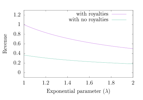
Figure 3: Creator revenue with optimal, $p_{0},r$ compared to that without royalties (optimal $p_{0}$ when $r=0$).

Royalties Expand Trade Under Information Asymmetry

As was the case in Section 4, by increasing creator utility, royalties also expand the space of parameters in which trade occurs between creator and speculator. Let $\mathbbm{T}$ be the set of parameters for which trade would occur if royalties were allowed, but would not occur in their absence.

Corollary 5 (Royalties expand the trade region under info. asymmetry).

Under information asymmetry, royalties increase the region of trade, that is, the set $\mathbbm{T}=\{\lambda,c\ |\ u_{c}^{*}\geq 0\ \cap u_{c,r=0}^{*}<0\ \lambda>0\ \cap c>0\}$ is non-empty. A visual representation is provided in Figure 4.

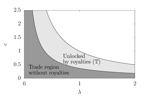
Figure 4: The region of trade unlocked by royalties under information asymmetry, in $\{\lambda,c\}$ space ($V\sim Exp[\lambda])$.

Key Takeaways from Section 5

To summarize, there are two key takeaways from this section which focuses on information asymmetry:

• Absent royalties, speculators use their informational advantage to extract end-buyer revenue for themselves, leaving creators and end-buyers worse off.

• Royalties shift the advantage back in the hands of the creator. They serve as a roundabout way to extract the benefits of dynamic pricing, even as mint prices remain static.

6 Royalties as a Price discrimination Mechanism

In this section, we remove risk aversion and information asymmetry, and focus instead on NFT collections. As mentioned in the introduction, NFTs are sometimes sold as multi-unit collections to a pool of possible buyers, where each item of the collection can be identical or have some variations. We expand our base model to capture a creator wishing to sell two NFTs to two end-buyers with uncertain valuations. As before, a speculator is also present. The analysis in this discrete $2\times 2$ case is already nontrivial — as we shall see, the game becomes combinatorial in nature. Nonetheless, this stylized case suffices to extract the main qualitative insights and shed some light on the economic forces at play.

At time 0, the creator sets a per-unit price, $p_{0}$, and royalty rate, $r$, for the collection, and the speculator chooses whether to buy 0, 1 or 2 units at the price $p_{0}$. At time $2$, the end-buyers arrive, and the speculator, as before, is assumed to be able to extract full end-buyer willingness-to-pay, selling the units at prices $v_{1}$ and $v_{2}$, respectively, where $v_{1},v_{2}\sim V$.

The core feature here is that the speculator can price discriminate, that is, he can sell the units at different prices, whereas the creator mints a single per-unit price, $p_{0}$, for the collection items. Note that this mimics the behavior of the majority of NFT collection drops in practice.

One interesting observation in this setup is that if the speculator buys both units, he can sell them for prices $v_{1},v_{2}$, so his expected revenue is $2E[V]$. Given there is no risk aversion and information asymmetry, one could think this collapses the game back to the base case of Theorem 1, where royalties can’t add value. In Theorem 1, the creator could set the price $p_{0}=E[V]$ with 0 royalties, and still extract all revenues for herself. Similarly here, the idea would be that she tries to obtain $E[V]$ for each unit, and recover $2E[V]$ in total. However, this simple strategy no longer works here because the speculator has the option of only buying a single NFT and selling it to the end-buyer with the highest valuation. This makes the equilibrium of the multi-unit game non-trivial and motivates the definition of Order Statistics.

Definition 2 (Order statistics).

Let $X_{1},\ldots,X_{n}$ be random variables. Define ${X}_{n,1},\ldots{X}_{n,n}$ to be the order statistics of $X_{1},\ldots,X_{n}$, in sorted order, i.e.,

$${X}_{n,1}\leq{X}_{n,2}\leq\cdots\leq{X}_{n,n}.$$ (12)

Though we only have two stochastic variables here, it is still useful to preserve this more general notation, given qualitative insights will hold for an arbitrary number of them.

With this definition ${X}_{n,1}=\min(X_{1},\ldots,X_{n})$, and ${X}_{n,n}=\max(X_{1},\ldots,X_{n})$. Notice that $X_{1}+\cdots+X_{n}={X}_{n,1}+\cdots+{X}_{n,n}$ because the order statistics are just a reordering of the random variables. In particular this means that

$$2E[V]=E[{V}_{2,1}]+E[{V}_{2,2}].$$ (13)

We are now equipped to solve the game via backward induction, meaning, we first need to characterize the speculator’s response, for given $p_{0}$, $r$. The speculator’s expected profits depend on how many NFTs he chooses to purchase. In particular, his profits are:

$$\begin{array}[]{rl}0&\mbox{ if $0$ NFTs are purchased }\\ (1-r)E[{V}_{2,2}]-p_{0}&\mbox{ if $1$ NFT is purchased }\\ 2((1-r)\cdot E[V]-p_{0})&\mbox{ if $2$ NFTs are purchased. }\end{array}$$ (14)

The pair-wise comparison between these three terms divides the possible space of $p_{0}$ into three regions, the “low-price” region (where the speculator buys both units), the “mid-price” region (where the speculator buys one unit), and the “high-price” region (where the speculator buys zero units). More specifically, the speculator purchases:

$$\begin{array}[]{lll}2\quad\mbox{ NFTs}&\mbox{ if $p_{0}\leq(1-r)\cdot E[{V}_{2,1}]$ }&\mbox{(low-price)}\\ 1\quad\mbox{ NFT}&\mbox{ if $(1-r)\cdot E[{V}_{2,1}]<p_{0}\leq(1-r)\cdot E[{V}_{2,2}]$ }&\mbox{(mid-price)}\\ 0\quad\mbox{ NFTs}&\mbox{ if $(1-r)\cdot E[{V}_{2,2}]<p_{0}$ }&\mbox{(high-price)},\\ \end{array}$$ (15)

where we have used the identity from Equation 13 in the first two lines.

In turn, anticipating the speculator’s optimal strategy, the creator’s expected profits are:

$$2p_{0}+2\cdot r\cdot E[V] p_{0}\leq(1-r)\cdot E[{V}_{2,1}]$$ if (low-price) (16)

$$p_{0}+r\cdot E[{V}_{2,2}]+p_{0}\cdot\Pr[{V}_{2,1}>p_{0}] (1-r)\cdot E[{V}_{2,1}]<p_{0}\leq(1-r)\cdot E[{V}_{2,2}]$$ if (mid-price) (17)

$$2p_{0}\cdot\Pr[V>p_{0}] (1-r)\cdot E[{V}_{2,2}]<p_{0} \mbox{(high-price)},$$ if (18)

where the first line is if the creator sells both NFTs to the speculator, the second line is when only 1 of the NFTs is sold to the speculator and the other may be sold to an end-buyer, and the last line is when both NFTs may be sold to an end-buyer.

The creator’s optimization problem is to maximize her expected revenues described in Equations 16,17, 18, over $p_{0}$ and $r$. Denote these $u_{c}^{*}$ (at the optimal $p_{0}^{*},r^{*}$) and let $u_{c,r=0}^{*}$ represent the creator’s optimal revenues without royalties, that is, the optimal $p_{0}^{*}$ when $r=0$.

Given the space partition, the objective does have not continuous derivatives everywhere, and first-order conditions are complex in this case. Nonetheless, we have the following general results. We first show that absent royalties, the creator cannot extract the maximum possible revenues from the two end-buyers.

Theorem 4.

If $V$ is non-degenerate, and royalties are ruled out, the creator selling two units cannot extract the maximum possible revenue, that is, $u^{*}_{c,r=0}<2E[V]$.

We then characterize the optimal solution and objective function when royalties ARE allowed, as well as the gap $\Delta$ that they generate compared to the case without royalties.

Theorem 5.

When creators are selling multi-unit collections, they can leverage royalties to “piggy-back” off speculators’ ability to price discriminate end-buyers. The creator can recover the maximum possible revenues by giving out her NFTs for free to the speculator ($p_{0}=0$), and relying exclusively on the future income generated by royalties. This strategy extracts the highest possible revenues to the creator, $u^{*}_{c}=2E[V]$ and yields her excess profits (compared to the case without royalties) of:

$$\Delta=2\operatorname{E}[V]-u_{c,r=0}^{*}>0.$$

We emphasize here, the result is driven neither by information asymmetry, nor risk aversion. Rather, it is a mere consequence of the fact that royalties allow the creator to “piggy-back” off the speculator’s access to the aftermarket, and his ability to charge different buyers different prices. In other words, royalties can be thought of as a roundabout way for creators to capture the benefits of price discrimination, even as collection units are all sold at the mint price.

As before, the magnitude of these benefits can be meaningful. To illustrate, we give below the benefit $\Delta$ for the exponential distribution. The relative revenue increase of including royalties (in % of the suboptimal policy), is given by

$$\mathcal{I}=\frac{\Delta}{u^{*}_{c,r=0}}.$$

Lemma 5 (Quantifying Gains, Exponential Distribution).

Suppose $V\sim Exp[\lambda]$. Then, the optimal creator revenues with royalties are $u^{*}_{c}=2E[V]=2/\lambda,$ and without royalties, they are $u^{*}_{c,r=0}=\frac{3}{2\lambda}\Big{(}1+e^{-3}\Big{)}$. This implies $\Delta=\frac{e^{3}-3}{2\lambda e^{3}}>0$, and $\mathcal{I}=\frac{e^{3}-3}{3(1+e^{3})}\sim 0.27$, that is, the use of royalties increases creator revenues by $27\%,\ \forall\lambda\in(1,\infty)$. This is illustrated in Figure 5.

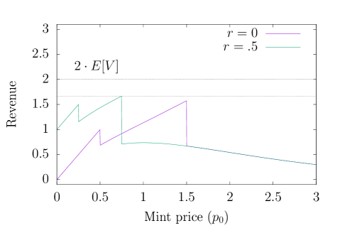
Figure 5: Creator revenues from Lemma 5 (with $\lambda=1$) as a function of mint price $p_{0}$, when the creator has 2 NFTs to sell. The optimal mint price in each case corresponds to the peak point.

Royalties Expand Trade for NFT Collections

As was the case in Sections 4 and 5, by increasing creator utility, royalties also expand the space of parameters in which trade occurs between creator and speculator. Let $\mathbbm{T}$ be the set of parameters for which trade would occur if royalties were allowed, but would not occur in their absence.

Corollary 6 (Royalties expand the trade region for NFT Collections).

When selling collections of multiple NFTs, royalties increase the region of trade, that is, the set $\mathbbm{T}=\{\lambda,c\ |\ u_{c}^{*}\geq 0\ \cap u_{c,r=0}^{*}<0\ \lambda>0\ \cap c>0\}$ is non-empty. A visual representation is provided in Figure 6.

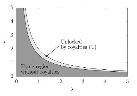
Figure 6: The region of trade unlocked by royalties when selling NFT Collections, in $\{\lambda,c\}$ space ($V\sim Exp[\lambda])$.

Key Takeaways from Section 6

To summarize, there are two key takeaways from this section which focuses on NFT collections:

• Absent royalties, the creator cannot extract the maximum NFT collection revenues from heterogeneous end-buyers.

• Royalties restore this possibility. They serve as a roundabout way to extract the benefits of price discrimination, even as collection items are all priced at the same fixed mint price.

7 Discussion & Concluding Thoughts

In this work, we have given three scenarios where creator royalties unlock additional, and often substantial benefits for creators. This helps to shed some light on the ongoing debate of whether marketplaces should enforce royalties. Our analysis suggests they can and do bring value to creators, in multiple different ways. Because they also improve trade propensity, they may be beneficial to the exchanges themselves (although a rigorous evaluation of exchange utility functions is not the focus of this paper and clearly beyond its scope).

Limitations and Evolution of the Royalty Model

As discussed in the introduction, one common criticism of NFT royalties is that they are not auto-enforceable. Enforcing (pro-rata) royalty payments is challenging because NFT contracts, as currently written, have no way of knowing the sale price. The contract is aware of the transfer of the NFT, but the actual payment can be handled in a separate transaction (or off-chain entirely). To see this problem clearly, imagine an NFT owner agrees to ‘sell” their NFT for a briefcase full of gold. The NFT contract has no knowledge of the gold, or its value unless participants explicitly tell the contract. Since royalties can only be assessed by someone with knowledge of the sale price, in practice, royalties have been enforced by the marketplaces. Thus, a creator who requests 10% royalties may see those royalties assessed if their NFT is sold on one exchange, but not if it’s sold on another.

Technically, it’s currently possible to enforce fixed royalties, i.e., a fixed payment to the creator at every subsequent transfer, but this does not allow the creators to capture any of the gains when their creations dramatically increase in value.

One proposal on the table is to propose a new asset class with self-enforcement of royalties, though there are some technical challenges. For example, Metaplex proposed a new NFT asset class that enforces on-chain creator royalties, and Magic Eden in the same vein suggested royalty-enforcing collectibles to be a class of its own coexisting with optional-royalty NFTs.

One can also think of alternatives to royalties. To capture some of the future value of their work, creators can hold back some of their inventory to sell later. This is the approach that Larva Labs took with their CryptoPunks. They released 9,000 CryptoPunks for free, and held back 1,000 to be sold at a later date Marcobello (2022). Of course, this has the disadvantage of not maximizing immediate cashflow for creators, who may be cash constrained.

Alternatively, working within the existing technical contracting constraints, we could imagine a probabilistic approach to allow creators to capture pro-rata royalties in expectation. Since NFT contracts are aware of transfers, it would be possible to create an NFT contract that probabilistically reverts back to the creator at every transfer. In more detail, every time the owner calls the transfer function, there would be a fixed probability (e.g. 5%) that the NFT is transferred back to the original creator instead of the intended recipient. Thus when a buyer purchased the NFT and the seller initiated the transfer, there would be some fixed probability that the NFT would transfer to the creator rather than the buyer. This mechanism would allow the creator to capture a percentage of the value of the NFT at each transfer in expectation. Unfortunately, this would also dramatically increase the variance of the value of the “royalty” payments, and is thus unlikely to be adopted.

Appendix A Proofs

Proof of Lemma 1.

Note that $\Pr[V>p_{0}]=1-F(p_{0})$, with $f,F$ being the density and cumulative distribution functions of $V$. Take the first and second-order derivatives of the objective function:

$$FOC\quad\Leftrightarrow \quad\frac{\partial}{\partial p_{0}}\Big{(}p_{0}(1-F(p_{0}))\Big{)}=1-F(p_{0})-p_{0}f(p_{0})=0$$ (19)

$$SOC\ Concavity\quad\Leftrightarrow \quad\frac{\partial^{2}}{\partial p_{0}^{2}}\Big{(}p_{0}(1-F(p_{0})\Big{)}=-2f(p_{0})-p_{0}f^{\prime}(p_{0})\leq 0.$$ (20)

From (20), concavity holds iff $p_{0}\geq-2\frac{f(p_{0})}{f^{\prime}(p_{0})}$. For example, this trivially holds for the uniform distribution given $f\geq 0$, $f^{\prime}=0$ and $p_{0}\geq 0$.

Concavity is too strict of a requirement for some other distributions, but in general, quasi-concavity, or at least uni-modality, suffice and will hold. In such cases, the first-order condition (19) implies that $p_{0}^{*}$ is the solution to:

$$p_{0}=\frac{1-F(p_{0})}{f(p_{0})}.$$

The right side can be interpreted as the inverse hazard rate (failure rate). A few examples: When $V$ is uniform between $[v_{L},v_{H}]$, $p_{0}^{*}=\frac{v_{H}}{2}$. When $V$ is exponential with parameter $\lambda$, the objective is unimodal and $p_{0}^{*}=\frac{1}{\lambda}$. When $V$ is normally distributed with parameters $\mu,\sigma$, the objective is unimodal and there is still a unique solution for $p_{0}^{*}$ but it is not in closed-form.

∎

Proof of Theorem 1.

When both the creator and the speculator are risk neutral, the creator’s maximization problem becomes

$$\max_{p_{0},r}\quad E\left[v_{c}\right]$$

$$\mbox{subject to:}\quad\mu(1-r)-p_{0}=0,$$

with $v_{c}=p_{0}+rp_{2}-c$, and $p_{2}=V$. Taking the expectation, $E[v_{c}]=p_{0}+r\mu-c$, the problem becomes

$$\max_{r\in[0,1]}\quad\mu(1-r)+r\mu-c,$$

which simplifies to $\max_{r}(\mu-c)=\mu-c$. The above is conditional on the creator preferring to sell the NFT to the speculator at time 1, rather than waiting with the hope of selling the NFT to the end-buyer at time $2$.

This follows from the Markov inequality argument in Corollary 1 (after noting $\mu-c=E[V]-c$). Intuitively, the creator prefers to sell the NFT to the speculator to “piggy-back” off of the speculator’s access to the aftermarket. ∎

Proof of Lemma 2.

Replacing the constraint (7) in the objective function simplifies the problem to a quadratic over $r$:

$$\max_{r}\mu-c-(\eta_{s}(1-r)^{2}+\eta_{c}r^{2})\sigma^{2}.$$ (21)

Solving and eliminating the non-feasible root gives the optimal royalty rate, $r$ as follows:

$$r^{*}=\frac{\eta_{s}}{\eta_{s}+\eta_{c}}.$$

Replacing this in (7) gives an optimal price of

$$p_{0}^{*}=\frac{\eta_{c}}{(\eta_{c}+\eta_{s})^{2}}\Big{(}(\eta_{c}+\eta_{s})\mu-\eta_{c}\eta_{s}\sigma^{2}\Big{)}.$$ (22)

Plugging these into the utility Equation 21 gives

$$\mu-c-(\eta_{s}(1-{r^{*}})^{2}+\eta_{c}{r^{*}}^{2})\sigma^{2} =\mu-c-\left(\eta_{s}\left(\frac{-\eta_{c}}{\eta_{c}+\eta_{s}}\right)^{2}+\eta_{c}\left(\frac{\eta_{s}}{\eta_{c}+\eta_{s}}\right)^{2}\right)\sigma^{2}$$

$$=\mu-c-\left(\frac{\eta_{c}\eta_{s}}{\eta_{c}+\eta_{s}}\right)\sigma^{2}.$$

∎

Proof of Theorem 2.

The creator profit with royalties is given in Equation 9, and the creator revenue without royalties is given in Equation 8. Thus we must show that

$$\mu-c-\left(\frac{\eta_{c}\eta_{s}}{\eta_{c}+\eta_{s}}\right)\sigma^{2}\geq\mu-c-\eta_{s}\sigma^{2}.$$ (23)

The difference is

$$\sigma^{2}\left(\eta_{s}-\frac{\eta_{c}\eta_{s}}{\eta_{c}+\eta_{s}}\right) =\sigma^{2}\left(\frac{\eta_{c}\eta_{s}+\eta_{s}^{2}-\eta_{c}\eta_{s}}{\eta_{c}+\eta_{s}}\right)$$ (24)

$$=\sigma^{2}\left(\frac{\eta_{s}^{2}}{\eta_{c}+\eta_{s}}\right).$$ (25)

which is positive whenever $\eta_{c}$ and $\eta_{s}$ are both positive. Thus the option of royalties leads to strictly higher utility for the seller whenever $\eta_{s}>0$ and $\eta_{c}+\eta_{s}>0$.

Comparative statics: Denote the difference in utilities between royalties and no-royalties as a function $f$ in three variables, namely $\eta_{s},\eta_{c},\sigma$, that is

$$f(\eta_{s},\eta_{c},\sigma)=\frac{\eta_{s}^{2}\sigma^{2}}{\eta_{s}+\eta_{c}}.$$ (26)

It is straightforward to check the first derivatives that if $\eta_{s},\eta_{c}>0$, then $f(\eta_{s},\eta_{c},\sigma)$ is increasing in $\eta_{s}$ and $\sigma$, but decreasing in $\eta_{c}$.

∎

Proof of Lemma 3.

As a first step, we can rewrite the creator’s objective function (10). Ignoring the constant $c$, we have

$$\Big{(}p_{0}+rE[V|(1-r)V\geq p_{0}]\Big{)}\cdot\Pr[(1-r)V\geq p_{0}]+p_{0}\Pr[(1-r)\cdot V<p_{0}\ \cap\ V\geq p_{0}]$$

$$=\left(p_{0}+rE\left[V~{}\middle|~{}(1-r)V\geq p_{0}\right]\right)\left(1-F\left(\frac{p_{0}}{1-r}\right)\right)+p_{0}\left(F\left(\frac{p_{0}}{1-r}\right)-F(p_{0})\right)$$

$$=\left(p_{0}+r\cdot\frac{\int_{\frac{p_{0}}{1-r}}^{\infty}vf(v)dv}{1-F\left(\frac{p_{0}}{1-r}\right)}\right)\left(1-F\left(\frac{p_{0}}{1-r}\right)\right)+p_{0}\left(F\left(\frac{p_{0}}{1-r}\right)-F(p_{0})\right)$$

$$=p_{0}\left(1-F\left(\frac{p_{0}}{1-r}\right)\right)+r\int_{\frac{p_{0}}{1-r}}^{\infty}vf(v)dv+p_{0}\left(F\left(\frac{p_{0}}{1-r}\right)-F(p_{0})\right)$$

$$=p_{0}(1-F(p_{0}))+r\int_{\frac{p_{0}}{1-r}}^{\infty}vf(v)dv$$

Thus the creator’s maximization problem is:

$$\max_{p_{0},r}p_{0}(1-F(p_{0}))+r\int_{\frac{p_{0}}{1-r}}^{\infty}vf(v)dv-c.$$

To find the first-order conditions on $p_{0}$, we can use Leibniz’s integral rule to obtain:

$$\frac{\partial}{\partial p_{0}}\left(p_{0}(1-F(p_{0}))+r\int_{\frac{p_{0}}{1-r}}^{\infty}vf(v)dv\right)=1-F(p_{0})-p_{0}f(p_{0})-\frac{p_{0}f\left(\frac{p_{0}}{1-r}\right)}{(1-r)^{2}}$$

and

$$\frac{\partial}{\partial r}\left(p_{0}(1-F(p_{0}))+r\int_{\frac{p_{0}}{1-r}}^{\infty}vf(v)dv\right)=\int_{\frac{p_{0}}{1-r}}^{\infty}vf(v)dv-\frac{rp_{0}^{2}f\left(\frac{p_{0}}{1-r}\right)}{(1-r)^{3}}.$$

∎

Proof of Theorem 3.

Starting with the expected creator revenue in Equation 10, the creator’s optimization problem is written as

$$\max_{p_{0},r}\quad\left(p_{0}+rE\left[V~{}\middle|~{}(1-r)V\geq p_{0}\right]\right)\cdot\Pr[(1-r)V\geq p_{0}]+p_{0}\Pr[(1-r)\cdot V<p_{0}\cap V\geq p_{0}]$$ (27)

Notice that

$$\Pr[(1-r)\cdot V<p_{0}\cap V\geq p_{0}]=\Pr[(1-r)V\leq p_{0}]-\Pr[V\leq p_{0}],$$ (28)

because

$$\Pr[(1-r)\cdot V<p_{0}\cap V\geq p_{0}] =\Pr[\{(1-r)\cdot V<p_{0}\}\cap\{V\geq p_{0}\}]$$

$$=\Pr[\{V<\frac{p_{0}}{1-r}\}\cap\{V\geq p_{0}\}]$$

$$=\Pr[V\leq\frac{p_{0}}{1-r}]-\Pr[V\leq p_{0}]$$

$$=\Pr[(1-r)V\leq p_{0}]-\Pr[V\leq p_{0}].$$

From there we use the above identity to simplify the objective function:

$$\left(p_{0}+rE\left[V~{}\middle|~{}(1-r)V\geq p_{0}\right]\right)\cdot\Pr[(1-r)V\geq p_{0}]+p_{0}\Pr[(1-r)\cdot V<p_{0}\cap V\geq p_{0}]$$

$$=\left(p_{0}+rE\left[V~{}\middle|~{}(1-r)V\geq p_{0}\right]\right)\cdot\Pr[(1-r)V\geq p_{0}]+p_{0}\left(\Pr[(1-r)V\leq p_{0}]-\Pr[V\leq p_{0}]\right)$$

$$=\left(p_{0}+rE\left[V~{}\middle|~{}(1-r)V\geq p_{0}\right]\right)\cdot\Pr[(1-r)V\geq p_{0}]+p_{0}\cdot\Pr[(1-r)V\leq p_{0}]-p_{0}\cdot\Pr[V\leq p_{0}]$$

$$=\left(p_{0}+rE\left[V~{}\middle|~{}(1-r)V\geq p_{0}\right]\right)\cdot\Pr[(1-r)V\geq p_{0}]+p_{0}\cdot\left(1-\Pr[(1-r)V\geq p_{0}]\right)-p_{0}\cdot\Pr[V\leq p_{0}]$$

$$=\left(p_{0}+rE\left[V~{}\middle|~{}(1-r)V\geq p_{0}\right]\right)\cdot\Pr[(1-r)V\geq p_{0}]+p_{0}-p_{0}\cdot\Pr[(1-r)V\geq p_{0}]-p_{0}\cdot\Pr[V\leq p_{0}]$$

$$=\left(rE\left[V~{}\middle|~{}(1-r)V\geq p_{0}\right]\right)\cdot\Pr[(1-r)V\geq p_{0}]+p_{0}-p_{0}\cdot\Pr[V\leq p_{0}]$$

$$=\left(rE\left[V~{}\middle|~{}(1-r)V\geq p_{0}\right]\right)\cdot\Pr[(1-r)V\geq p_{0}]+p_{0}\cdot\left(1-\Pr[V\leq p_{0}]\right)$$

which yields a simplified objective function:

$$p_{0}\cdot\Pr[V>p_{0}]+r\cdot E\left[V~{}\middle|~{}(1-r)V\geq p_{0}\right]\cdot\Pr[(1-r)V\geq p_{0}].$$ (29)

Now, notice that setting $p_{0}=0$, and $r=1$, the creator earns revenue $E[V]$, which is the maximum amount of revenue that could be achieved. For this solution to be unique, we need to verify what happens if the creator chooses an $r<1$.

When $r<1$, the creator’s revenue is

$$p_{0}\int_{p_{0}}^{\infty}f_{V}(v)dv+r\int_{\frac{p_{0}}{1-r}}^{\infty}vf_{V}(v)dv =p_{0}\int_{p_{0}}^{\frac{p_{0}}{1-r}}f_{V}(v)dv+\int_{\frac{p_{0}}{1-r}}^{\infty}(rv+p_{0})f_{V}(v)dv$$

$$\leq p_{0}\int_{p_{0}}^{\frac{p_{0}}{1-r}}f_{V}(v)dv+\int_{\frac{p_{0}}{1-r}}^{\infty}vf_{V}(v)dv$$

$$\leq\int_{p_{0}}^{\infty}vf_{V}(v)dv$$ (30)

$$=E[V]-\int_{0}^{p_{0}}vf_{V}(v)dv.$$ (31)

Now, consider three cases $\Pr[V<p_{0}]>0$, $\Pr\left[p_{0}<V<\frac{p_{0}}{1-r}\right]>0$ and $\Pr[V>p_{0}]>0$.

Case 1: If $\Pr[V<p_{0}]>0$, then

$$\int_{0}^{p_{0}}vf_{V}(v)dv>0.$$

By Equation 31, the creator revenue is bounded by

$$E[V]-\int_{0}^{p_{0}}vf_{V}(v)dv<E[V].$$

Case 2: If $\Pr\left[p_{0}<V<\frac{p_{0}}{1-r}\right]$, then

$$p_{0}\int_{p_{0}}^{\frac{p_{0}}{1-r}}f_{V}(v)dv<\int_{p_{0}}^{\frac{p_{0}}{1-r}}vf_{V}(v)dv.$$

So by Equation A, the creator revenue is bounded by

$$p_{0}\int_{p_{0}}^{\frac{p_{0}}{1-r}}f_{V}(v)dv+\int_{\frac{p_{0}}{1-r}}^{\infty}(rv+p_{0})f_{V}(v)dv <\int_{p_{0}}^{\frac{p_{0}}{1-r}}vf_{V}(v)dv+\int_{\frac{p_{0}}{1-r}}^{\infty}(rv+p_{0})f_{V}(v)dv$$

$$\leq\int_{p_{0}}vf_{V}(v)dv$$

$$\leq E[V].$$

Case 3: If $\Pr\left[V>\frac{p_{0}}{1-r}\right]$, then

$$\int_{\frac{p_{0}}{1-r}}^{\infty}(rv+p_{0})f_{V}(v)dv<\int_{\frac{p_{0}}{1-r}}^{\infty}vf_{V}(v)dv.$$

So by Equation A, the creator’s revenue is bounded by

$$p_{0}\int_{p_{0}}^{\frac{p_{0}}{1-r}}f_{V}(v)dv+\int_{\frac{p_{0}}{1-r}}^{\infty}(rv+p_{0})f_{V}(v)dv <p_{0}\int_{p_{0}}^{\frac{p_{0}}{1-r}}f_{V}(v)dv+\int_{\frac{p_{0}}{1-r}}^{\infty}vf_{V}(v)dv$$

$$\leq\int_{p_{0}}^{\infty}vf_{V}(v)dv$$

$$\leq E[V].$$

Therefore, in all three situations, the creator cannot achieve revenue $E[V]$. Thus the unique optimal solution is $r=1,p_{0}=0$.

∎

Proof of Lemma 4.

First, we show that if $V$ is exponentially distributed with parameter $\lambda$, then

$$\Pr[V(1-r)>p_{0}]=e^{-\lambda\frac{p_{0}}{1-r}}$$ (32)

and

$$E\left[V~{}\middle|~{}V(1-r)>p_{0}\right]=\frac{p_{0}}{1-r}+E[V].$$ (33)

To see this, consider that $V$ exponentially distributed implies

$$\Pr[V>p_{0}]=e^{-\lambda p_{0}}$$

so

$$\Pr[V(1-r)>p_{0}]=e^{-\lambda\frac{p_{0}}{1-r}}.$$

Equation 33 follows from the memoryless property of exponential distributions, i.e.,

$$E\left[V~{}\middle|~{}V(1-r)>p_{0}\right] =\frac{\int_{\frac{p_{0}}{1-r}}^{\infty}x\lambda e^{-\lambda x}dx}{\Pr[(1-r)\cdot V>p_{0}]}$$

$$=e^{\lambda\frac{p_{0}}{1-r}}\int_{\frac{p_{0}}{1-r}}^{\infty}x\lambda e^{-\lambda x}dx$$

$$=e^{\lambda\frac{p_{0}}{1-r}}\left(e^{-\lambda\frac{p_{0}}{1-r}}\cdot\frac{\left(\lambda\frac{p_{0}}{1-r}+1\right)}{\lambda}\right)$$

$$=\frac{p_{0}}{1-r}+\frac{1}{\lambda}$$

$$=\frac{p_{0}}{1-r}+E[V].$$

Plugging Equations 32 and 33 into Equation 29, the creator revenue becomes

$$r\cdot\left(\frac{p_{0}}{1-r}+\frac{1}{\lambda}\right)\cdot e^{-\lambda\frac{p_{0}}{1-r}}+p_{0}e^{-\lambda p_{0}}.$$ (34)

From here, setting $r=0$ gives the optimal revenues absent royalties, $p_{0}e^{-\lambda p_{0}}$. Setting $p_{0}=0$ and $r=1$ gives the optimal revenues with royalties, $1/\lambda$. All other results follow trivially from here.

∎

Proof of Theorem 4.

It suffices to show that the creator cannot achieve revenue $2E[V]$ in any of the three regimes.

Low-price: $p_{0}<E[{V}_{2,1}]$. In this regime, the creator revenue is $2p_{0}$, so the maximum creator revenue is $2\left(E[{V}_{2,1}]\right)$.

Mid-price: $E[{V}_{2,1}]<p_{0}<E[{V}_{2,2}]$. In this regime, the creator revenue is $p_{0}+p_{0}\cdot\Pr[{V}_{2,1}>p_{0}]$. Now, Markov’s inequality tells us that $p_{0}\cdot\Pr[{V}_{2,1}>p_{0}]<E[{V}_{2,1}]$. Since $p_{0}\leq E[{V}_{2,2}]$ in the mid-price regime, then

$$p_{0}+p_{0}\cdot\Pr[{V}_{2,1}>p_{0}]<E[{V}_{2,2}]+E[{V}_{2,1}]=2E[V]$$ (35)

High-price: $E[{V}_{2,2}]<p_{0}$. In this regime, the creator revenue is $2p_{0}\cdot\Pr[V>p_{0}]$, which by Markov’s inequality is bounded by $2E[V]$.

∎

Proof of Theorem 5.

Since the creator’s revenue is defined piecewise, we analyze the three regions (low-price, mid-price, high-price) separately.

Low-price: First, notice that the creator revenue is linearly increasing in $p_{0}$ in the low-price regime ($p_{0}<(1-r)\cdot E[{V}_{2,1}]$).

In the low-price regime (i.e., when $p_{0}<(1-r)\cdot E[{V}_{2,1}]$), the creator’s maximum profit is

$$2p_{0}+2\cdot r\cdot E[V] \leq 2\left((1-r)\cdot E[{V}_{2,1}]\right)+2\cdot r\cdot E[V]$$ (36)

$$=(1-r)E[{V}_{2,1}]+\left((1-r)E[{V}_{2,1}+r\left(E[{V}_{2,1}]+E[{V}_{2,2}]\right)\right)$$ (37)

$$=(2-r)E[{V}_{2,1}]+rE[{V}_{2,2}].$$ (38)

This is strictly increasing in $r$. Thus the creator can set $p_{0}=0$ $r=1$, to obtain revenue $2E[V]$, which is the maximum possible.

Mid-price: In the mid-price regime (i.e., when $(1-r)\cdot E[{V}_{2,1}]<p_{0}<(1-r)\cdot E[{V}_{2,2}]$) the creator profit is

$$p_{0}+r\cdot E[{V}_{2,2}]+p_{0}\cdot\Pr[{V}_{2,1}>p_{0}] \leq(1-r)\cdot E[{V}_{2,2}]+r\cdot E[{V}_{2,2}]+p_{0}\cdot\Pr[{V}_{2,1}>p_{0}]$$ (39)

$$=E[{V}_{2,2}]+p_{0}\cdot\Pr[{V}_{2,1}>p_{0}]$$ (40)

In the mid-price regime, by Lemma 7, $p_{0}\cdot\Pr[{V}_{2,1}>p_{0}]<E[{V}_{2,1}]$, so the creator cannot obtain revenue $2E[V]$ in the mid-price regime.

High-price:

In the high-price regime (i.e., when $(1-r)\cdot E[{V}_{2,2}]<p_{0})$, the creator profit is

$$2p_{0}\cdot\Pr[V>p_{0}]$$ (41)

By Lemma 7, if $V$ is non-degenerate, the Markov bound is loose so

$$2p_{0}\cdot\Pr[V>p_{0}]<2E[V]$$ (42)

so if $V$ is non-degenerate, the creator cannot obtain the revenue $2E[V]$ in the high-price regime.

Thus in if $V$ is non-degenerate, the unique optimal strategy is for the creator to set $p_{0}=0$ and $r=1$. In this case, the creator obtains revenue $2E[V]$ (which is the maximum achievable from 2 buyers with valuation $V$).

∎

Proof of Lemma 5.

We treat the two cases, without royalties, and with royalties, separately.

Proof of Lemma 5 - With Royalties

Consider the creator revenues in each of the three regimes.

In the low-price regime, the creator revenue is $2p_{0}+2\cdot r\cdot E[V]$, which is linearly increasing in $p_{0}$. Thus setting $p_{0}=(1-r)\cdot E[{V}_{2,1}]$ strictly dominates any smaller $p_{0}$.

In the mid-price regime, the creator revenue is

$$p_{0}+r\cdot E[{V}_{2,2}]+p_{0}\cdot P[{V}_{2,1}>p_{0}] =p_{0}+rE[{V}_{2,2}]+p_{0}(1-F_{V}(p_{0}))^{2}$$ (43)

Looking at the first derivative:

$$\frac{\partial}{\partial p_{0}}\left(p_{0}(1+(1-F_{V}(p_{0})))^{2}+rE[{V}_{2,2}]\right) =1+(1-F_{V}(p_{0}))^{2}-2p_{0}f_{V}(p_{0})(1-F_{V}(p_{0}))$$ (44)

Thus revenues in the mid-price regime will be increasing in $p_{0}$ whenever

$$1+(1-F_{V}(p_{0}))^{2}-2p_{0}f_{V}(p_{0})(1-F_{V}(p_{0}))>0$$ (45)

Now $(1-F_{V}(p_{0}))=e^{-\lambda p_{0}}$, and $f_{V}(p_{0})=\lambda e^{-\lambda p_{0}}$, so

$$1+(1-F_{V}(p_{0}))^{2}-2p_{0}f_{V}(p_{0})(1-F_{V}(p_{0})) =1+e^{-2\lambda p_{0}}-2\lambda p_{0}e^{-2\lambda p_{0}}$$ (46)

$$=1+e^{-2\lambda p_{0}}(1-2\lambda p_{0})$$ (47)

Note, $(1-x)\cdot e^{-x}$ is minimized at $x=2$, where the value is $e^{-2}$, thus $1+e^{-2\lambda p_{0}}(1-2\lambda p_{0})>0$ for all $p_{0}$. Which means that the creator revenue is increasing in $p_{0}$ throughout the mid-price regime. Thus setting $p_{0}=(1-r)\cdot E[{V}_{2,2}]$ yields the highest revenue in the mid-price regime.

Finally, we consider the high-price regime, which is defined as the region where $p_{0}>(1-r)E[{V}_{2,2}]$. Now ${V}_{2,1}$ is distributed as an exponential with parameter $2\lambda$, so $E[{V}_{2,1}]=\frac{1}{2\lambda}$. Thus

$$E[{V}_{2,2}]=2E[V]-E[{V}_{2,1}]=\frac{2}{\lambda}-\frac{1}{2\lambda}=\frac{3}{2\lambda}$$ (48)

Thus the high-price regime is the region where $p_{0}>(1-r)\frac{3}{2}\lambda$.

In the high-price regime, creator revenues are $2p_{0}\cdot\Pr[V>p_{0}]$, which, for the exponential distribution becomes

$$2p_{0}e^{-\lambda p_{0}}.$$ (49)

Differentiating with respect to $p_{0}$, we have

$$2(1-\lambda p_{0})\cdot e^{-\lambda p_{0}}$$ (50)

which is maximized when $p_{0}=\frac{1}{\lambda}$. When $r<\frac{2}{3}$, $p_{0}=\frac{1}{\lambda}$, is in the high-price regime, otherwise, the maximum occurs at the boundary, i.e., $p_{0}=(1-r)\frac{3}{2\lambda}$.

Thus if $r<\frac{2}{3}$, the maximum occurs at $p_{0}=(1-r)E[{V}_{2,2}]$. If $r>\frac{2}{3}$, we need to compare $p_{0}=(1-r)E[{V}_{2,2}]$ with the revenue obtained at $p_{0}=\frac{1}{\lambda}$.

The maximum value in the low-price regime is given by $p_{0}=(1-r)E[{V}_{2,1}]=\frac{1-r}{2\lambda}$, and the revenue is

$$\frac{1-r}{\lambda}e^{-\frac{1-r}{2}}$$ (51)

When $p_{0}=(1-r)\cdot E[{V}_{2,2}]$, the revenue is

$$p_{0}\cdot(1+\Pr[{V}_{1,2}>p_{0}])+rE[{V}_{2,2}] =E[{V}_{2,2}]+p_{0}\cdot\Pr[{V}_{2,1}>p_{0}]$$ (52)

$$=\frac{3}{2\lambda}+p_{0}\Pr[V>p_{0}]^{2}$$ (53)

$$=\frac{3}{2\lambda}+p_{0}e^{-2\lambda p_{0}}$$ (54)

$$=\frac{3}{2\lambda}+\frac{3(1-r)}{2\lambda}e^{-3\cdot(1-r)}$$ (55)

When $p_{0}=\lambda$, and $p_{0}=\frac{1}{\lambda}$ is in the high-price regime, the revenue is

$$2p_{0}e^{-\lambda p_{0}}=\frac{2}{\lambda e}$$ (56)

So for a fixed $r$, the creator has three possible choices:

$$\mbox{Set }p_{0}=(1-r)E[{V}_{2,1}]\mbox{ with revenue } \frac{1-r}{\lambda}e^{-\frac{1-r}{2}}$$ (57)

$$\mbox{Set }p_{0}=(1-r)E[{V}_{2,2}]\mbox{ with revenue } \frac{3}{2\lambda}\left(1+(1-r)e^{-3(1-r)}\right)$$ (58)

$$\mbox{Set }p_{0}=\frac{1}{\lambda}>(1-r)E[{V}_{2,2}]\mbox{ with revenue } \frac{2}{\lambda e}$$ (59)

Notice that

$$\frac{1-r}{\lambda}e^{-\frac{1-r}{2}}\leq\frac{1}{\lambda}<\frac{3}{2\lambda}<\frac{3}{2\lambda}\left(1+(1-r)e^{-3(1-r)}\right)$$ (60)

So the creator always prefers setting the price $p_{0}$ to the upper-end of the mid-price regime over the upper end of the low-price regime. Next, notice that

$$\frac{3}{2\lambda}\left(1+(1-r)e^{-3(1-r)}\right)>\frac{2}{\lambda e}$$ (61)

So the creator will always prefer the upper end of the mid-price regime to any point in the high-price regime.

Thus any fixed $r\in[0,1)$, the creator’s optimal strategy is to set $p_{0}=(1-r)\cdot E[{V}_{2,2}]$ and receive revenue

$$\frac{3}{2\lambda}\left(1+(1-r)e^{-3(1-r)}\right)$$ (62)

This is maximized when $r=\frac{2}{3}$, and in this setting, the creator revenue is

$$\frac{3\left(1+\frac{1}{3e}\right)}{2\lambda}$$ (63)

Note that

$$\frac{3\left(1+\frac{1}{3e}\right)}{2\lambda}<\frac{3\left(1+\frac{1}{3}\right)}{2\lambda}=2E[V]$$ (64)

So the creator cannot obtain revenue $2E[V]$ except by setting $r=1$.

Proof of Lemma 5 - Without Royalties

If $V$ is exponentially distributed with parameter $\lambda$, then $E[V]=\frac{1}{\lambda}$, $E[{V}_{2,1}]=\frac{1}{2\lambda}$, and $E[{V}_{2,2}]=2E[V]-E[{V}_{2,1}]=\frac{3}{2\lambda}$.

In the low-price regime (when $p_{0}<E[{V}_{2,1}]$) the creator revenue is $2p_{0}$.

In this case, the maximum revenue is

$$2E[{V}_{2,1}]=\frac{1}{\lambda}$$ (65)

In the mid-price regime (when $E[{V}_{2,1}]<p_{0}<E[{V}_{2,2}]$) the creator revenue is $p_{0}\cdot(1+\Pr[{V}_{2,1}>p_{0}])$.

$$p_{0}\cdot(1+\Pr[{V}_{2,1}>p_{0}])=p_{0}\cdot(1+e^{-2\lambda p_{0}})$$ (66)

This function is increasing in $p_{0}$, so it is maximized at the right-hand boundary, i.e., when $p_{0}=\frac{3}{2\lambda}$

In this case, the revenue is $\frac{3}{2\lambda}\cdot(1+e^{-3})$

In the high-price regime (when $E[{V}_{2,2}]<p_{0}$) the creator revenue is $2p_{0}\cdot\Pr[V>p_{0}]$.

$$2p_{0}\cdot\Pr[V>p_{0}]=2p_{0}e^{-\lambda p_{0}}$$ (67)

This is maximized when $p_{0}=\frac{1}{\lambda}$, which is outside the high-price regime. Inside the high-price regime, this function is strictly decreasing, so the maximum value in the high-price regime occurs on the left boundary, i.e., $p_{0}=\frac{3}{2\lambda}$.

In this case, the revenue is $\frac{3}{\lambda\cdot e^{\frac{3}{2}}}$

Since

$$\frac{3(1+e^{-3})}{2\lambda}>\frac{1}{\lambda}>\frac{3e^{-\frac{3}{2}}}{\lambda}$$ (68)

The maximum creator revenue is achieved by setting

$$p_{0}=\frac{3}{2\lambda},$$ (69)

in which case, the speculator purchases only 1 of the 2 NFTs, and the creator have expected revenues:

$$\frac{3}{2\lambda}\cdot(1+e^{-3}).$$

The rest of the results of the Lemma follow trivially from here.

∎

Appendix B Additional Technical Lemmas for Section 6

Lemma 6.

If $V$ is a non-negative, non-degenerate random variable, then Markov’s inequality is loose, i.e.,

$$v\Pr[V>v]<E[V]$$ (70)

for all $v$.

Proof of Lemma 6.

Since $V$ is non-degenerate, there exists points $0<v_{1}<v_{2}$ and a value $\epsilon$, with $0<\epsilon<(v_{2}-v_{1})/2$, such that $\Pr[v_{1}-\epsilon<V<v_{1}+\epsilon]>0$, and $\Pr[v_{2}-\epsilon<V<v_{2}+\epsilon]>0$

Let $\delta\stackrel{{\scriptstyle\mathrm{def}}}{{=}}\min\left(\Pr[v_{1}-\epsilon<V<v_{1}+\epsilon],\Pr[v_{2}-\epsilon<V<v_{2}+\epsilon]\right)$. Then, $\delta>0$.

Now, consider two cases: Case 1: If $v\leq v_{1}+\epsilon$, then

$$E[V]-v\cdot\Pr[V>v] =\int_{0}^{\infty}xf_{V}(x)dx-v\int_{v}^{\infty}f_{V}(x)dx$$ (71)

$$\geq\int_{v_{2}-\epsilon}^{v_{2}+\epsilon}(x-v_{1})f_{V}(x)dx$$ (72)

$$\geq(v_{2}-\epsilon-v_{1})\int_{v_{2}-\epsilon}^{v_{2}+\epsilon}f_{V}(x)dx$$ (73)

$$\geq(v_{2}-\epsilon-v_{1})\delta$$ (74)

$$>0$$ (75)

Case 2: If $v_{1}+\epsilon<v$, then

$$E[V]-v\cdot\Pr[V>v] =\int_{0}^{\infty}xf_{V}(x)dx-v\int_{v}^{\infty}f_{V}(x)dx$$ (76)

$$\geq\int_{0}^{v_{1}+\epsilon}xf_{V}(x)dx$$ (77)

$$\geq\int_{v_{1}-\epsilon}^{v_{1}+\epsilon}xf_{V}(x)dx$$ (78)

$$\geq(v_{1}-\epsilon)\delta$$ (79)

$$>0$$ (80)

∎

Lemma 7.

If $V$ is a non-negative, non-degenerate random variable, then ${V}_{n,k}$ is a non-negative, non-degenerate random variable for all $1\leq k\leq n$, and hence Markov’s Inequality is loose.

Proof of Lemma 7.

By assumption, there exists points $0<v_{1}<v_{2}$ and a value $\epsilon$, with $0<\epsilon<(v_{2}-v_{1})/2$, such that $\Pr[v_{1}-\epsilon<V<v_{1}+\epsilon]>0$, and $\Pr[v_{2}-\epsilon<V<v_{2}+\epsilon]>0$ Let $\delta\stackrel{{\scriptstyle\mathrm{def}}}{{=}}\min\left(\Pr[v_{1}-\epsilon<V<v_{1}+\epsilon],\Pr[v_{2}-\epsilon<V<v_{2}+\epsilon]\right)$. Then, $\delta>0$.

With probability at least $\delta^{n}$, all $n$ draws of $V$ land in the region $[v_{i}-\epsilon,v_{i}+\epsilon]$, so

$$\Pr[v_{i}-\epsilon<{V}_{n,k}<v_{i}+\epsilon]>\delta^{n}>0$$ (81)

Since this holds for $i\in\left\{1,2\right\}$, ${V}_{n,k}$ is non-degenerate.

By Lemma 6, that means

$$\max_{p_{0}}p_{0}\cdot\Pr[{V}_{n,k}>p_{0}]<E[{V}_{n,k}]$$ (82)

In other words, the Markov bound is loose for ${V}_{n,k}$. ∎

Appendix C Model Extension: Risk Aversion with Differing Market Views

In this section, we extend the model outlined in Section 4, to consider the case where the buyer and the speculator have different ideas about the future value of the asset.

C.1 Model

As in Section 4, the participants’ profits are:

$$v_{c} =p_{0}+rV-c\quad\mbox{(Creator profit)}$$ (83)

$$v_{s} =(1-r)V-p_{0}\quad\mbox{(Speculator profit)}$$ (84)

and, as in Section 4, we assume the creator and the speculator are both subject to mean-variance utility

$$u_{c} =E[v_{c}]-\eta_{c}\operatorname{Var}[v_{c}]\quad\mbox{(Creator utility)}$$ (85)

$$u_{s} =E[v_{s}]-\eta_{s}\operatorname{Var}[v_{s}]\quad\mbox{(Speculator utility)}$$ (86)

The modification comes about in the maximization problem. The creator’s goal is to find the sale price $p_{0}$, and the royalty rate $r$ that maximizes the following equations:

$$\max_{p_{0},r}\quad E\left[v_{c}\right]-\eta_{c}\operatorname{Var}[v_{c}]$$ (87)

$$\mbox{subject to:}\quad\mu_{s}(1-r)-p_{0}-\eta_{s}\sigma_{s}^{2}(1-r)^{2}=0$$ (88)

Equations 87 and 88 are the analogues of Equations 4 and 5 in Section 4. The only difference is that now the creator has the view that $E[V]=\mu_{c}$ and $\operatorname{Var}(V)=\sigma_{c}^{2}$, whereas the speculator takes the view that $E[V]=\mu_{s}$, and $\operatorname{Var}(V)=\sigma_{s}^{2}$. We do not assume any Bayesian updating between the creator and the speculator – they simply have conflicting views about the future.

C.2 Risk neutrality

When both participants are risk neutral (i.e., $\eta_{c}=\eta_{s})$ we can prove an analog of Theorem 1 in Section 4.

Theorem 6 (Risk-neutrality).

Note that if both the creator and speculator are risk neutral ($\eta_{s}=\eta_{c}=0$), then the creator profit is

$$\mu_{s}(1-r)+r\mu_{c}-c$$ (89)

which is independent of $r$ whenever $\mu_{s}=\mu_{c}$.

Proof.

When both the creator and the speculator are risk neutral, the creator’s maximization problem becomes

$$\max_{p_{0},r}\quad E\left[v_{s}\right]$$ (90)

$$\mbox{subject to:}\quad\mu_{s}(1-r)-p_{0}=0$$ (91)

Since $E[v_{s}]=p_{0}+r\mu_{c}-c$, the problem becomes

$$\max_{r\in[0,1]}\quad\mu_{s}(1-r)+r\mu_{c}-c$$ (92)

which yields $r^{*}=0$ if $\mu_{s}>\mu_{c}$ and $r^{*}=1$ if $\mu_{s}<\mu_{c}$, and is independent of $r$ if $\mu_{s}=\mu_{c}$. ∎

Thus in the risk-neutral setting, with only a single item, Theorem 1 shows that royalties are effectively “priced in” and do not confer any advantage to the creator.

C.3 Risk aversion

When the creator and the speculator are risk-averse, (i.e., $\eta_{c},\eta_{s}>0$), we show the nonzero royalties can lead to higher utility (and profits) for the creator.

From the creator’s perspective

$$E[v_{c}] =p_{0}+r\mu_{c}-c$$ (93)

$$\operatorname{Var}[v_{c}] =r^{2}\sigma_{c}^{2}$$ (94)

So Equation 87 become

$$E\left[v_{s}\right]-\eta_{c}Var_{s}[v_{s}]=p_{0}+r\mu_{c}-c-\eta_{c}r^{2}\sigma_{c}^{2}$$ (95)

Rearranging Equation 88, we have

$$p_{0}=\mu_{s}(1-r)-\eta_{s}\sigma_{s}^{2}(1-r)^{2}$$ (96)

So the creator’s maximization problem (Equations 4 & 5) becomes

$$\max_{r}\quad p_{0}+r\mu_{c}-c-\eta_{c}r^{2}\sigma_{c}^{2}$$ (97)

$$\mbox{subject to:}\quad p_{0}=\mu_{s}(1-r)-\eta_{s}\sigma_{s}^{2}(1-r)^{2}$$ (98)

Solving this quadratic gives the optimal royalty rate, $r$

$$r^{*}=\frac{1}{2}\frac{(\mu_{c}-\mu_{s})+2\eta_{s}\sigma_{s}^{2}}{\eta_{s}\sigma_{s}^{2}+\eta_{c}\sigma_{c}^{2}}\quad\mbox{(c.f. Equation~{}\ref{eqn:optr}) }$$ (99)

As an example, when all parameters are set to equal 1, the optimal $r=1/2$.

Note that if no royalties were allowed, and the creator makes a take-it-or-leave-it offer, then the maximum price the speculator is willing to pay is $\mu_{s}-\eta_{s}\sigma_{s}^{2}$. If the creator charges this price, then the creator’s revenue is

$$\mu_{s}-\eta_{s}\sigma_{s}^{2}-c$$ (100)

As the creator chooses the optimal royalty rate, we state and prove the formal result:

Theorem 7.

The option of royalties always yields a higher utility for the creator.

Proof.

First, Equation 97 in $r=r^{*}$ minus Equation 8 yields

$$(p_{0}+r^{*}\mu_{c}-c-\eta_{c}{r^{*}}^{2}\sigma_{c}^{2})-(\mu_{s}-\eta_{s}\sigma_{s}^{2}-c)$$

Expanding in $p_{0},r^{*}$ by Equation 7 and Equation 9 yields

$$p_{0}+(r^{*}\mu_{c}-\mu_{s})+(\eta_{s}\sigma_{s}^{2}-\eta_{c}{r^{*}}^{2}\sigma_{c}^{2})$$

$$=\eta_{s}\sigma_{s}^{2}-\mu_{s}-\frac{\eta_{c}\sigma_{c}^{2}\left(2\eta_{s}\sigma_{s}^{2}-\mu_{s}+\mu_{c}\right){}^{2}}{4\left(\eta_{s}\sigma_{s}^{2}+\eta_{c}\sigma_{c}^{2}\right){}^{2}}$$

$$+\frac{\mu_{c}\left(2\eta_{s}\sigma_{s}^{2}-\mu_{s}+\mu_{c}\right)}{2\left(\eta_{s}\sigma_{s}^{2}+\eta_{c}\sigma_{c}^{2}\right)}$$

$$+\mu_{s}\left(1-\frac{2\eta_{s}\sigma_{s}^{2}-\mu_{s}+\mu_{c}}{2\left(\eta_{s}\sigma_{s}^{2}+\eta_{c}\sigma_{c}^{2}\right)}\right)$$

$$-\eta_{s}\sigma_{s}^{2}\left(1-\frac{2\eta_{s}\sigma_{s}^{2}-\mu_{s}+\mu_{c}}{2\left(\eta_{s}\sigma_{s}^{2}+\eta_{c}\sigma_{c}^{2}\right)}\right){}^{2}$$

Rearrange the terms, we get

$$(p_{0}+r\mu_{c}-c-\eta_{c}r^{2}\sigma_{c}^{2})-(\mu_{s}-\eta_{s}\sigma_{s}^{2}-c)=\frac{\left(2\eta_{s}\sigma_{s}^{2}-\mu_{s}+\mu_{c}\right){}^{2}}{4\left(\eta_{s}\sigma_{s}^{2}+\eta_{c}\sigma_{c}^{2}\right)}$$

Observe that by assumption, the speculator and creator are risk averse (i.e., $\eta_{s},\eta_{c}>0)$, so that we know both the numerator and the denominator are positive, thus, we know

$$(p_{0}+r\mu_{c}-c-\eta_{c}r^{2}\sigma_{c}^{2})-(\mu_{s}-\eta_{s}\sigma_{s}^{2}-c)>0$$

which precisely implies that the option of royalties yields a higher utility for the creator, as desired.

∎

By Theorem 7, we know the difference between royalties and no royalties is

$$\frac{\left(2\eta_{s}\sigma_{s}^{2}-\mu_{s}+\mu_{c}\right){}^{2}}{4\left(\eta_{s}\sigma_{s}^{2}+\eta_{c}\sigma_{c}^{2}\right)}\geq 0$$

Comparative statics: Denote the difference in utilities between royalties and no-royalties as a function $f$ in six variables, namely $\mu_{s},\mu_{c},\eta_{s},\eta_{c},\sigma_{s},\sigma_{c}$, that is

$$f(\mu_{s},\mu_{c},\eta_{s},\eta_{c},\sigma_{s},\sigma_{c})=\frac{\left(2\eta_{s}\sigma_{s}^{2}-\mu_{s}+\mu_{c}\right){}^{2}}{4\left(\eta_{s}\sigma_{s}^{2}+\eta_{c}\sigma_{c}^{2}\right)}$$ (101)

We analyze the utility gain of the creator associated with royalties in relation to other variables, analogous to Theorem 2 as in Section 4. First, we claim some facts regarding the first derivatives of utility gain $f$:

Lemma 8.

The difference in creator between the royalty and no-royalty model increases in speculator uncertainty ($\sigma_{s}$) if and only if

$$-2\eta_{s}\sigma_{s}^{2}-4\eta_{c}\sigma_{c}^{2}\leq\mu_{s}-\mu_{c}\leq 2\eta_{s}\sigma_{s}^{2}$$ (102)

Proof.

We consider $\frac{\partial f}{\partial\sigma_{s}}$, that is

$$\frac{\partial f}{\partial\sigma_{s}}=\frac{\eta_{s}\sigma_{s}\left(2\eta_{s}\sigma_{s}^{2}-\mu_{s}+\mu_{c}\right)\left(2\eta_{s}\sigma_{s}^{2}+\mu_{s}+4\eta_{c}\sigma_{c}^{2}-\mu_{c}\right)}{2\left(\eta_{s}\sigma_{s}^{2}+\eta_{c}\sigma_{c}^{2}\right){}^{2}}$$

Since the denominator (as well as $\eta_{s}\sigma_{s}$) is positive, $\frac{\partial f}{\partial\sigma_{s}}$ will be positive if and only if

$$\left(2\eta_{s}\sigma_{s}^{2}-(\mu_{s}-\mu_{c})\right)\left(2\eta_{s}\sigma_{s}^{2}+4\eta_{c}\sigma_{c}^{2}+(\mu_{s}-\mu_{c})\right)\geq 0$$

This holds if and only if

$$-2\eta_{s}\sigma_{s}^{2}-4\eta_{c}\sigma_{c}^{2}\leq\mu_{s}-\mu_{c}\leq 2\eta_{s}\sigma_{s}^{2}$$ (103)

∎

Lemma 9.

As creator uncertainty ($\sigma_{c}$) increases, the difference between creator utility in the royalty and no-royalty models decreases.

Proof.

We need to show that difference between Equations 6 and Equation 8 is decreasing in $\sigma_{c}$. Consider $\frac{\partial f}{\partial\sigma_{c}}$, that is

$$\frac{\partial f}{\partial\sigma_{c}}=-\frac{\eta_{c}\sigma_{c}\left(2\eta_{s}\sigma_{s}^{2}-\mu_{s}+\mu_{c}\right){}^{2}}{2\left(\eta_{s}\sigma_{s}^{2}+\eta_{c}\sigma_{c}^{2}\right){}^{2}}$$

Note that besides the square terms, $\eta_{c}$ is positive by assumption, so that $\frac{\partial f}{\partial\sigma_{c}}$ is negative, which proves the claim. ∎

Having analyzed the first derivative of utility gain, we state a formal result parallel to Theorem 2 as in section 4:

Theorem 8 (Risk Aversion).

Under risk aversion, assume different market views, creator royalties increase creator utility by $\frac{\left(2\eta_{s}\sigma_{s}^{2}-\mu_{s}+\mu_{c}\right){}^{2}}{4\left(\eta_{s}\sigma_{s}^{2}+\eta_{c}\sigma_{c}^{2}\right)}\geq 0$, compared to no-royalty case. Further, the utility gains associated with royalties

• increases if and only if $-2\eta_{s}\sigma_{s}^{2}-4\eta_{c}\sigma_{c}^{2}\leq\mu_{s}-\mu_{c}\leq 2\eta_{s}\sigma_{s}^{2}$

• decreases as creator uncertainty, $\sigma_{c}$, increases

Proof.

The proof follows directly from Lemma 8 and Lemma 9. ∎

As Lemma 9 indicates the utility gain decreases as the creator becomes more uncertain about future price (i.e., $\sigma_{c}$ increases), we show creator’s utility in fact decreases under this setting:

Theorem 9.

As creator uncertainty ($\sigma_{c}$) increases, creator utility decreases (unless the creator is risk-seeking ($\eta_{c}<0$), in which case creator utility is increasing in $\sigma_{c}$).

Proof.

First, we denote the creator utility according to Equation 6 as a function in $\mu_{s},\mu_{c},\eta_{s},\eta_{c},\sigma_{s},\sigma_{c}$, that is

$$g(\mu_{s},\mu_{c},\eta_{s},\eta_{c},\sigma_{s},\sigma_{c})=p_{0}+r^{*}\mu_{c}-c-\eta_{c}{r^{*}}^{2}\sigma_{c}^{2}$$

Expanding in $p_{0},r^{*}$ with respect to Equation 7 and Equation 9, we get

$$g(\mu_{s},\mu_{c},\eta_{s},\eta_{c},\sigma_{s},\sigma_{c})=\frac{-4c\eta_{s}\sigma_{s}^{2}-4\eta_{c}\sigma_{c}^{2}\left(\eta_{s}\sigma_{s}^{2}-\mu_{s}+c\right)+\mu_{s}^{2}+4\eta_{s}\sigma_{s}^{2}\mu_{c}-2\mu_{s}\mu_{c}+\mu_{c}^{2}}{4\left(\eta_{s}\sigma_{s}^{2}+\eta_{c}\sigma_{c}^{2}\right)}$$

Take the partial of $g$ with respect to $\sigma_{c}$, we get

$$\frac{\partial g}{\partial\sigma_{c}} =-\frac{\eta_{c}\sigma_{c}\left(2\eta_{s}\sigma_{s}^{2}-\mu_{s}+\mu_{c}\right){}^{2}}{2\left(\eta_{s}\sigma_{s}^{2}+\eta_{c}\sigma_{c}^{2}\right){}^{2}}$$

Suppose the creator is risk-averse, then we know $\eta_{c}\sigma_{c}$ is positive. Therefore, $\frac{\partial g}{\partial\sigma_{c}}$ is negative, so that $g$ decreases in $\sigma_{c}$. If the creator is risk-seeking, then $\eta_{c}\sigma_{c}$ is negative, so that $\frac{\partial g}{\partial\sigma_{c}}$ is positive. In this case, $g$ increases in $\sigma_{c}$, as desired.

∎

References

- (1)
- Ante (2021) Ante, L. (2021), ‘The non-fungible token (NFT) market and its relationship with Bitcoin and Ethereum’, Available at SSRN 3861106 .
- Benhaim et al. (2022) Benhaim, A., Falk, B. H. & Tsoukalas, G. (2022), ‘Scaling blockchains: Can committee-based consensus help?’, Working Paper .
- Burks et al. (2020) Burks, Z., Morgan, J., Malone, B. & Seibel, J. (2020), ‘EIP-2981: NFT royalty standard’, https://eips.ethereum.org/EIPS/eip-2981.
-
Cachon & Swinney (2009)
Cachon, G. P. & Swinney, R. (2009), ‘Purchasing, pricing, and quick response in the presence of strategic
consumers’, Management Science 55(3), 497–511.
http://www.jstor.org/stable/40539162 - Carreras (2022) Carreras, T. (2022), ‘Art Gobbler NFTs top $20,000 within minutes of free mint’, https://cryptobriefing.com/art-gobbler-nfts-top-20000-within-minutes-of-free-mint/.
- Cong et al. (2021) Cong, L. W., Li, Y. & Wang, N. (2021), ‘Tokenomics: Dynamic adoption and valuation’, The Review of Financial Studies 34(3), 1105–1155.
- Gan et al. (2021) Gan, J., Tsoukalas, G. & Netessine, S. (2021), ‘Initial coin offerings, speculation, and asset tokenization’, Management Science 67(2), 914–931.
- Gan et al. (2022) Gan, R., Tsoukalas, G. & Netessine, S. (2022), ‘Financing platforms with cryptocurrency: Token retention, sales commission, and ico caps’, Available at SSRN 3776411 .
- Geron (2022) Geron, T. (2022), ‘Otherside’s utterly avoidable NFT disaster’, https://www.protocol.com/newsletters/protocol-fintech/otherside-yuga-labs-ethereum.
- Hayward (2022a) Hayward, A. (2022a), ‘Another NFT marketplace goes zero royalties in ’race to the bottom”, https://decrypt.co/113021/nft-marketplace-looksrare-zero-royalties.
- Hayward (2022b) Hayward, A. (2022b), ‘Loot, one year later: The NFT hype is dead—but ’Lootverse’ hope lives on’, https://decrypt.co/108354/loot-one-year-later-nft-hype-dead-lootverse-hope-lives-on.
- Kent (2021) Kent, C. (2021), ‘Artists have been attempting to secure royalties on their work for more than a century. blockchain finally offers them a breakthrough’, https://news.artnet.com/opinion/artists-blockchain-resale-royalties-1956903.
- Kireyev (2022) Kireyev, P. (2022), ‘NFT marketplace design and market intelligence’, https://papers.ssrn.com/sol3/papers.cfm?abstract_id=4002303.
- Lovo & Spaenjers (2018) Lovo, S. & Spaenjers, C. (2018), ‘A model of trading in the art market’, American Economic Review 108(3), 744–74.
- Marcobello (2022) Marcobello, M. (2022), ‘CryptoPunks, CryptoCats and CryptoKitties: How they started and how they’re going’, https://www.coindesk.com/learn/cryptopunks-cryptocats-and-cryptokitties-how-they-started-and-how-theyre-going/.
- Murray (2022) Murray, M. D. (2022), ‘NFTs rescue resale royalties? the wonderfully complicated ability of NFT smart contracts to allow resale royalty rights’, https://papers.ssrn.com/sol3/papers.cfm?abstract_id=4164029.
- Nadini et al. (2021) Nadini, M., Alessandretti, L., Di Giacinto, F., Martino, M., Aiello, L. M. & Baronchelli, A. (2021), ‘Mapping the NFT revolution: market trends, trade networks, and visual features’, Scientific reports 11(1), 1–11.
- Nelson (2022) Nelson, D. (2022), ‘Solana goes dark for 7 hours as bots swarm ‘candy machine’ NFT minting tool’, https://www.coindesk.com/tech/2022/05/01/solana-goes-dark-for-7-hours-as-bots-swarm-candy-machine-nft-minting-tool/.
- NFTStatistics.eth (2022) NFTStatistics.eth (2022), Deep dives: NFT royalties, Technical report, proof.xyz.
- NonFungible.com (2022) NonFungible.com (2022), Q3 nft market report 2022, Technical report, NonFungible.com.
- Qadir & Parker (2022) Qadir, S. & Parker, G. (2022), NFT royalties: The $1.8bn question, Technical report, Galaxy Digital.
- Saleh (2021) Saleh, F. (2021), ‘Blockchain without waste: Proof-of-stake’, The Review of financial studies 34(3), 1156–1190.
- Su (2010) Su, X. (2010), ‘Optimal pricing with speculators and strategic consumers’, Management Science 56(1), 25–40.
- Tsoukalas & Falk (2020) Tsoukalas, G. & Falk, B. H. (2020), ‘Token-weighted crowdsourcing’, Management Science 66(9), 3843–3859.
- van Haaften-Schick & Whitaker (2022) van Haaften-Schick, L. & Whitaker, A. (2022), ‘From the artist’s contract to the blockchain ledger: New forms of artists’ funding using equity and resale royalties’, Journal of Cultural Economics pp. 1–29.
- Vasan et al. (2022) Vasan, K., Janosov, M. & Barabási, A.-L. (2022), ‘Quantifying NFT-driven networks in crypto art’, Scientific Reports 12(1), 1–11.
- Whitaker & Kräussl (2020) Whitaker, A. & Kräussl, R. (2020), ‘Fractional equity, blockchain, and the future of creative work’, Management Science 66(10), 4359–4919.