Interval Valued Fuzzy Modeling and Indirect Adaptive Control of Quadrotor

Abstract

In this paper, a combination of fuzzy clustering estimation and sliding mode control is used to control a quadrotor system, whose mathematical model is complex and has unknown elements, including structure, parameters, and so on. In addition, they may be affected by external environmental disturbances. At first, the nonlinear unknown part of the system is estimated by a fuzzy model, A new method is presented for constructing a Takagi-Sugeno (TS) interval-valued fuzzy model (IVFM) based on input-output data of the identified system. Following the construction of the fuzzy model that estimates the unknown part of the quadrotor system, a control and on-line adjusting of the fuzzy modeled part of dynamics is used. In this step, the system model will be estimated in adaptive form so that the dynamic equations can be used in sliding mode control. Finally, the proposed technique is applied, and the simulation results are presented to show the effectiveness of this approach in controlling the quadrotor with unknown nonlinear dynamics.

Keywords Interval values Modeling  $\cdot$ fuzzy clustering  $\cdot$ fuzzy control  $\cdot$ Indirect adaptive control  $\cdot$ quadrotor control $\cdot$ sliding mode control  $\cdot$ type-2 fuzzy sets.

1 Introduction

The quadrotor unmanned aerial vehicle (UAV) is a typical second-order, nonlinear, strongly coupled dynamic system. An adaptive control scheme is significant for unmanned quadrotor helicopters, and this has received attention in the literature. External disturbances can have a impact on the stability and reliability of these systems. Therefore, it is very important to study the effects of system disturbances and design control strategies that address actuator faults and disturbances. To date, many methods and strategies have been presented in the literature H.Mo and Farid (2019). Authers presents PD control as well as a fuzzy adaptive PD control scheme in which the controller’s gains are automatically adjusted in relation to the error signal rate Gao et al. (2015). The fuzzy adaptive PD controller is quicker at achieving the desired response as compared to the other one. The authors of Rabhi et al. (2011) used a robust fuzzy control approach to stabilize a quadrotor’s attitude angles. They used the parallel distributed compensation technique to design the fuzzy controller. High-order sliding mode observer was designed to provide state information required for fuzzy controller design. The study Niroumand and Seyedsajadi (2013), integrated integral backstepping with fuzzy logic to improve the flight controller’s performance. Simulation results show superior performances for the fuzzy-integral backstepping approach over conventional integral backstepping.  Fuzzy based sliding mode control for quadrotor UAV has recently been reported in Pazooki and Mazinan (2017) and control structure is augmented via a genetic algorithm for optimization purposes. This approach can be further investigated using second order sliding mode control to avoid chattering. In Ul Amin and Kamsin (2017), NRBF and E-RBF are used collectively to approximate the unknown dynamics of the quadrotor. A study Dierks and Jagannathan (2010), addresses online learning of the dynamics of a quadrotor nonlinear model through neural networks. Online learning is normally preferred over offline learning for the reason that quadrotors may fly in a dynamic environment where different worse case perturbations may occur, and such operating scenarios are hard to generate offline. Also, this study conveys the idea of using NNs to control the six degrees of freedom of a quadrotor along with designing an ANN observer to estimate states of the system. A neural network is used to approximate unmodeled dynamics during flight in Dierks and Jagannathan (2009), and interconnection errors in flight formation are investigated. in Li and Zheng (2016) the position controller considered as nonlinear system and approximated using radial basis function neural networks, This study is unique in a sense that a complete controller is approximated via adaptive rule and trained online. This neuronal network-based controller provides adaptation for parametric uncertainties along with other external disturbances.  In Lee (2021) authors proposed a nonlinear-sliding-surface-based SMC for tracking and stabilization with an SMO. To improve the performance of the quadrotor system, they remodeled the augmented quadrotor dynamics and estimated the unmeasured states and their derivatives through the sliding mode observer. To improve the SMC control performance, a nonlinear sliding surface is used to reduce the convergence time with a modified deceleration curve. The authors proved the performance of a tracking system. Based on the above research analysis, we propose an adaptive control strategy, and design an adaptive controller for a quadrotor UAVs in the presence of external and internal disturbances. The introduced adaptive control strategy is based on fuzzy logic control theory and adaptive sliding mode theory. A new method for constructing a Takagi-Sugeno (TS) type-2 fuzzy model offline, based on input-output data, is proposed, and the obtained fuzzy model of the dynamic is used to build the model-based control of the system. with an adaptive control strategy scheme that compensates the effects of the disturbance and an unmodeled dynamics control system. The system’s global asymptotic stability is validated by the Lyapunov function. The effectiveness and feasibility of the proposed method are demonstrated by simulation studies of the unmanned vehicle. The rest of the paper is organized as follows. Section  2 describes the proposed method of IVFM construction from input-output datasets of the system. Section  3 presents the application of the proposed method to build the IVFM of the quadrotor. Section  4 presents the proposed control strategy based on fuzzy logic control and adaptive sliding mode for the quadrotor UAV under external disturbances and parameter changes. The stability analysis of the new methodology is validated by the Lyapunov function. The results of simulation studies that demonstrate the performance of the proposed adaptive fuzzy schemes are presented in Section  5. Finally, general conclusions and future work plans are provided.

2 Fuzzy modeling

The proposed method for constructing a Takagi-Sugeno (TS) type-2 fuzzy model, based on the input-output data of the identified system is constructed in three steps: (1) structure identification by fuzzy clustering; (2) envelope detection; and (3) parameter identification. In the structure identification phase, a clustering method based on the Gustafson-Kessel algorithm (GKCA) is used in order to detect the linear subsystems of the whole nonlinear system Babuska et al. (1998) (local linearization). Then, an envelope detection algorithm (EDA) based on the derivative concept is proposed to estimate both the upper and lower membership functions of the type-2 fuzzy membership function (T2MF) defined point-wise. In the parameter identification step, the least squares algorithm is applied to compute the best parameter values for the premises (Gaussians) and the consequences (straight lines) parameters.

2.1 Fuzzy Clustering overview

Clustering is the partitioning of data into subsets or groups based on similarities between the data. The main potential of clustering is to detect the underlying structure in data, not only for classification and pattern recognition, but for model reduction and optimization. To detect clusters of different geometrical shapes in a single data set, we used the Fuzzy Gustafson Kessel Clustering (FGK), which extends the standard fuzzy c-means algorithm by employing an adaptive distance norm Babuska and Verbruggen (1997); Gustafson and Kessel (1979); Filho and Serra (2016) . Each cluster has its own norm-inducing matrix, $A_{i}$, which yields the inner-product norm Eqn. (1) shown below:

$$D_{ikA}^{2}=({\mathbf{x}}_{k}-{\mathbf{v}}_{i})^{T}{A_{i}}({\mathbf{x}_{k}}-\mathbf{v}_{i}),$$ (1)

where $1\leq i\leq c,1\leq k\leq N$ . The matrices $A_{i}$ are used as optimization variables in the $C-means$ functional, which will allow to each cluster to adapt the distance norm to the local topological structure of the data. Let $A$ denote a c-tuple of the norm-inducing matrices: $A=({A_{1}},{A_{2}},...,{A_{c}})$. The objective functional of the GK algorithm is defined by:

$$J(\mathbf{X},\mathbf{U\;,V,A})=\sum\limits_{i=1}^{c}\sum\limits_{k=1}^{N}{(\mu_{ik})}^{m}\textnormal{D}_{ikA}^{2}$$ (2)

where $N$ the number of data points, $c$ the number of clusters, $x_{k}$ the $k^{th}$ data point, ${v_{i}}$ the $i^{th}$ cluster center, ${\mu_{ik}}$ the degree of membership of the $k^{th}$ data in the $i^{th}$ cluster, $A_{i}$ the norm-inducing matrix of the $i^{th}$ cluster and $m$ is a weighting exponent that determines the fuzziness of the resulting clusters (typically $m=2$). In our paper, the GKCA is applied in order to obtain the fuzzy partition matrix $U={[\mu_{ik}]_{c\times N}}$, with ${\mu_{ik}}\in[{0\,\,1}]$ a membership degree.

2.2 Proposed envelope detection and estimation algorithm

The individual partitioning subsets ${\mu_{ik}}$ projected on the regressor $X$ will define directly fuzzy regions, in which the data can be reasonably approximated by linear sub-models defined by clusters. Projection data can also make the fuzzy system easy to read by humans

2.2.1 Detection of lower and upper premise MF

In order to detect the fuzzy premise MFs (lower MF $\underline{f}$ and the upper MF $\bar{f}$) we propose in what follows an approach called for Envelope Detection Algorithm (EDA) based on derivative concept. The algorithm is described in the following algorithm:

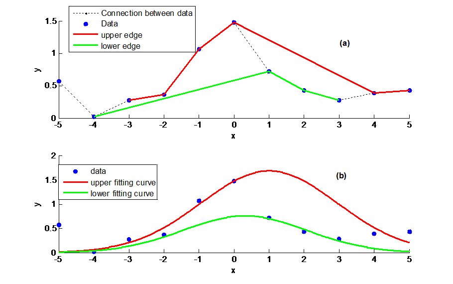
1) First, we interpolate the points linearly (dotted curve in Fig. 1 (a). between all segments $[y(i),y({i+1})]$ where $i$ represents the data indices.

The third-level of heading follows the style of the second-level heading. 2) We compute the slops between each successive data points $[y(i),y(i+1)]$ as:

$$d\left({i+1}\right)=\frac{y\left({i+1}\right)-y\left(i\right)}{x\left({i+1}\right)-x\left(i\right)}$$ (3)

3) Two cases can arise:

• When the slop $d$ in interval $[x(i),x(i+1)]$ is positive, then the point is considered as higher membership point and memorized with its indices as $(I_{h},y_{h}(I_{h}))$, where $I_{h}=i+1$ represents the indices of the corresponding higher membership point $y_{h}$ s.t. $y_{h}(I_{h})=y(i+1)$.
  

• Otherwise, when the slop $d$ in interval $[x(i),x(i+1)]$ is negative, then the point is considered as lower membership point and memorized with its indices as $(I_{L},y_{L}(I_{L}))$, where $I_{L}=i+1$ represents the indices of the corresponding lower membership point $y_{L}$ s.t. $y_{L}(I_{L})=y(i+1)$.

By applying our method cited above, we show in Fig. 1 the shape of the obtained upper and lower envelopes, which represent the upper and lower type-2 MFs. The details of this technique are given in EDA Algorithm Bouhentala et al. (2017). This algorithm doesn’t ensure the separation of envelopes; to do that, we can apply the same algorithm again for both the upper and lower sets. When we apply this algorithm to the initial set of points, we get two sets:$\underline{f}$ and $\overline{f}$. Next, we use the same algorithm for both sets $(\underline{f}and\overline{f})$   to get another four sets. The proposed algorithm can be presented as the algorithm described here :

1. Applying ADE(initial set) gives two sets $(\underline{f},\overline{f})$

2. make $i=j=1$

3. $(\underline{f}_{j},{\bar{f}}_{i})=ADE($ initial set $)$

4. Calculate the upper set ${\bar{f}}$

   1. Make $i=i+1$

   2. $({\underline{f}}_{i},{\bar{f}}_{i})=ADE(\bar{f})$

   3. If go to step (a) else next:

   4. $\bar{f}={\bar{f}_{i}}$

5. Calculate the lower set

   1. Make $j=j+1$

   2. $({\underline{f}}_{j},{\bar{f}}_{j})=ADE(\underline{f})$

   3. If $j\neq j_{\max}$ go to step $(a)$ else next:

   4. $\underline{f}={\underline{f}_{j}}$

Figure 1: (a) Data envelope detection (b) Gaussian fitting

Figure 2: (a) with first applying EDA one time,(b) envelope fitting with Gaussian model

Figure 3: (c) after applying EDA two times, there are less intersection points (d) after Gaussian fitting, there is no intersection.

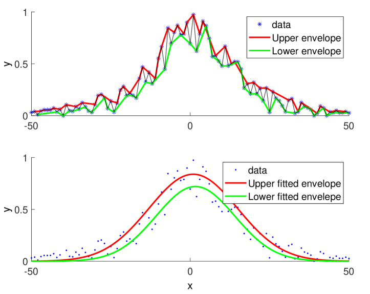
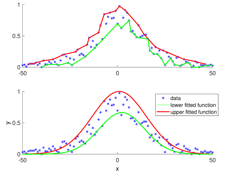
Look to the next example where the initial function is a Gaussian with added noise to create a cloud to its shape, in the Fig. 2 where the first ADE is applied and its corresponding fitting result as shown in the figure (b) there are many interactions points in different regions while the applying of EDA again make the envelopes less interacted and its fitted part show that our the final fitted functions envelops much points of the initial cloud Fig. 3 (d).

2.3 Constructing fuzzy models from partitions

At this step, we have two data sets of points: data set 1 represents the data of  $f_{L}$ and data set 2 represents the data of $f_{U}$ . Gaussian membership functions will be used in this investigation for the premise MF; thus, data sets 1 and 2 will be fitted to Gaussian models, yielding the lower and upper Gaussian membership functions $\bar{f}$ and $\underline{f}$. Until now, we have obtained, by using the proposed method, type-2 fuzzy Gaussian membership functions for the premises. The global model can be conveniently represented as a set of affine Takagi-Sugeno (TS) rules $R_{i}$  as follows:

$${if}x{is}{\tilde{A}_{i}}{then}\,{y_{i}}={a_{i}}x+{b_{i}}\,{for}i=1,2,...,c$$ (4)

where $x$ is the input, and $y$ is the output, ${\tilde{A}_{i}}=[\underline{f_{i}},\bar{f_{i}}]$ the $i^{th}$ obtained antecedent type-2 fuzzy MF. The consequent parameters $a_{i}$ and $b_{i}$ are estimated from the data using least square method.

3 Fuzzy modeling of unknown dynamics of quadrotor

In the following application, we will use the method presented above to model the unknown functions using input-output data, and then we will use those initial models to build the adaptive control.

3.1 Dynamic model of Quadrotor

Let’s consider the system in Eqn. (5) as presented in Lee (2021); Bouabdallah (2007) in which the state representation $\underline{x}=(\varphi,\dot{\varphi},\theta,\dot{\theta},\psi,\dot{\psi},x,\dot{x},y,\dot{y},z,\dot{z})$ is the state vector and $U=\left[{{U_{\phi}}\,{U_{\theta}}\,{U_{\psi}}\,{U_{z}}}\right]$ is the control vector. The transformation matrix between the rate of change of the orientation angles $(\dot{\varphi},\dot{\theta},\dot{\psi})$ and the body angular velocities $\left({p,q,r}\right)$ can be considered as unity matrix if the perturbations from hover flight are small. Then, one can write $(\dot{\varphi},\dot{\theta},\dot{\psi})\approx\left({p,q,r}\right)$ Bouabdallah (2007). Each axis can be approximately decoupled and controlled independently when the angular velocities are low and the attitude angle changes in small range. The drone parameters are shown in the Table 1.

$${\dot{x}=\left(\begin{array}[]{*{20}{c}}{\dot{\phi}}\\ {\dot{\theta}\dot{\psi}{a_{1}}+\dot{\theta}{a_{2}}{\Omega_{r}}+{b_{1}}{U_{1}}}\\ {\dot{\theta}}\\ {\dot{\phi}\dot{\psi}{a_{3}}+\dot{\phi}{a_{4}}{\Omega_{r}}+{b_{2}}{U_{2}}}\\ {\dot{\psi}}\\ {\dot{\theta}\dot{\phi}{a_{5}}+{b_{3}}{U_{3}}}\\ {\dot{z}}\\ {g-(\cos\phi\cos\theta)\frac{U_{z}}{m}}\\ {\dot{x}}\\ {{u_{x}}\tfrac{U_{z}}{m}}\\ {\dot{y}}\\ {{u_{y}}\tfrac{U_{z}}{m}}\end{array}\right)\\ }$$ (5)

$$\left.\begin{array}[]{*{20}{c}}{a_{1}}=({I_{yy}}-{I_{zz}})/{I_{xx}}\\ {a_{2}}={J_{r}}/{I_{xx}\hfill}\\ {a_{3}}=({I_{zz}}-{I_{xx}})/{I_{yy}}\\ {a_{4}}={J_{r}}/{I_{yy}\hfill}\\ {a_{5}}=({I_{xx}}-{I_{yy}})/{I_{zz}}\\ \end{array}\right|\begin{array}[]{*{20}{c}}b_{1}=l/I_{xx}\\ b_{2}=l/I_{yy}\\ b_{3}=1/{I_{zz}}\\ u_{x}=(\operatorname{c}\phi\operatorname{s}\theta\operatorname{c}\psi-\operatorname{s}\phi\operatorname{s}\psi)\\ u_{y}=(\operatorname{c}\phi\operatorname{s}\theta\operatorname{s}\psi-\operatorname{s}\phi\operatorname{c}\psi)\end{array}$$

Table 1: Parameters of the Quadrotor

$I_{zz}=0.09kg.m^{2}$	$m=1.2kg$	$l=0.23m$
$I_{yy}=0.18kg.m^{2}$	$d=1.1e-6N.m.s^{2}$	$g=9.81m.s^{-}2$
$I_{xx}=0.18kg.m^{2}$	$b=54.2e-6N.m^{2}$	$j_{r}=1.32e^{-}3kg.m^{2}$

the moment and force caused by the propeller are proportional to the square of the angular velocity. The inputs of each axis can be composed of the speed of the propeller and described as Bouabdallah (2007):

$$\left.\begin{array}[]{*{20}{c}}U_{\phi}=(\Omega_{1}-\Omega_{3})\\ U_{\theta}=(\Omega_{4}-\Omega_{2})\\ \end{array}\right|\begin{array}[]{*{20}{c}}U_{\phi}=(\Omega_{1}+\Omega_{3}-\Omega_{2}-\Omega_{4})\\ U_{z}=(\Omega_{1}+\Omega_{2}+\Omega_{3}+\Omega_{4})\\ \end{array}$$

3.2 Interval values Fuzzy modeling

The model Eqn. (5) can be decomposed into three subsystems:

$$\left({\begin{array}[]{*{20}{c}}{{{\dot{x}}_{1}}}\\ {{{\dot{x}}_{2}}}\end{array}}\right)=\left({\begin{array}[]{*{20}{c}}{\dot{\phi}}\\ {{f_{\phi}}(\dot{\theta},\dot{\psi})+{g_{1}}{U_{1}}}\end{array}}\right)$$ (6)

$$\left({\begin{array}[]{*{20}{c}}{{{\dot{x}}_{3}}}\\ {{{\dot{x}}_{4}}}\end{array}}\right)=\left({\begin{array}[]{*{20}{c}}{\dot{\theta}}\\ {{f_{\theta}}+{g_{2}}{U_{2}}}\end{array}}\right)$$ (7)

$$\left({\begin{array}[]{*{20}{c}}{{{\dot{x}}_{5}}}\\ {{{\dot{x}}_{6}}}\end{array}}\right)=\left({\begin{array}[]{*{20}{c}}{\dot{\psi}}\\ {{f_{\psi}}+{g_{3}}{U_{3}}}\end{array}}\right)$$ (8)

where $f_{\phi}(\dot{\theta},\dot{\psi},{\Omega_{r}})=\dot{\phi}\dot{\psi}{a_{1}}+\dot{\phi}{a_{2}}{\Omega_{r}}$ ,$f_{\theta}(\dot{\theta},\dot{\psi},{\Omega_{r}})=\dot{\theta}\dot{\phi}{a_{3}}+\dot{\theta}{a_{4}}{\Omega_{r}}$ ,$f_{\psi}(\dot{\theta},\dot{\psi},{\Omega_{r}})=\dot{\theta}\dot{\psi}{a_{5}}$ and ${g_{\phi}}={b_{1}}$ ,${g_{\theta}}={b_{2}}$ , ${g_{\psi}}={b_{3}}$. The parameters $g_{1}$, $g_{2}$ ,$g_{3}$ and the functions $f_{\phi}$, $f_{\theta}$ and $f_{\psi}$ are considered as unknown functions, and they will be estimated as follow :

the first step is to identify the functions ${f_{i}}(x,\dot{\psi},{\Omega_{r}})$ and ${g_{i}}$ where $\left\{{i=\phi,\theta,\psi}\right\}$ using clustering. ${\hat{f}_{i}}$ can be written as an TS approximation of the form IVFM Eqn. (4) :

$$\begin{array}[]{*{20}{l}}{f_{\phi}(x)={{\hat{f}}_{\phi}}({x_{8}},{x_{12}},{\Omega_{r}},{\theta_{f_{\phi}}})+\varepsilon={\theta_{{f_{\phi}}}}^{T}{\varphi_{f_{\phi}}}({x})}\\ {f_{\theta}(x)={{\hat{f}}_{\theta}}({x_{10}},{x_{12}},{\Omega_{r}},{\theta_{f_{\theta}}})+\varepsilon={\theta_{{f_{\theta}}}}^{T}{\varphi_{{f_{\theta}}}}(x)}\\ {f_{\psi}(x)={{\hat{f}}_{\psi}}({x_{10}},{x_{12}},{\theta_{f_{\psi}}})+\varepsilon={\theta_{{f_{\psi}}}}^{T}{\varphi_{{f_{\psi}}}}(x)}\end{array}$$

where $\theta_{f_{i}}={\left[{{\underline{w}}_{l}}^{T},{{\underline{w}}_{r}}^{T}\right]_{i}}^{T}$ and ${\underline{\psi}}_{f_{i}}(x,\dot{x})=\frac{1}{2}{\left[{{{\underline{\xi}}_{l}}^{T}(x,\dot{x}),{{{\underline{\xi}}}_{r}}^{T}(x,\dot{x})}\right]_{i}}^{T}$.

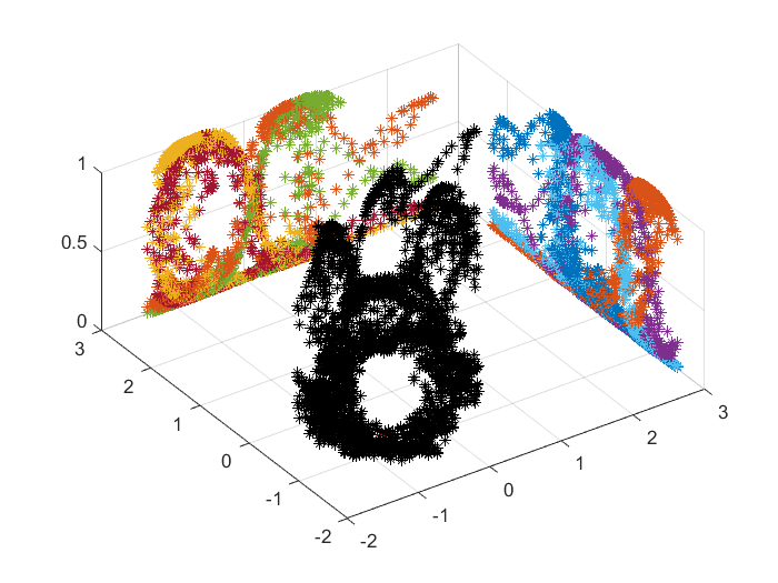
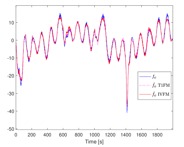
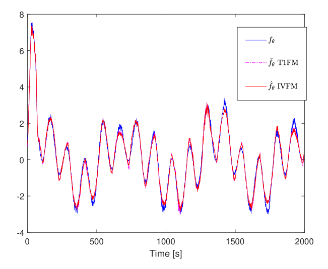
To collect input-output data, we generate two sets of data, one for identification by clustering, and the second for  validation. We start with a sequence of $4000$ samples ($2000$ for identification and $2000$ for validation) The sampling time is $T=0.01s$ with normal noise ($05\%$ of amplitude) is added to every output. The obtained data is treated using EDA in order to construct the membership functions as presented in Fig. 4. The membership functions type-1 and type-2 obtained with simulation data for ${f_{\phi}}({x},\Omega),{f_{\theta}}({x},\Omega)$ and ${f_{\psi}}({x},\Omega)$ are depicted in The figures (Fig. 5,  7), respectively.

Figure 4: Projection and construction of membership functions

Figure 5: Membership Functions of ${\hat{f}_{\phi}}(\underline{x})$

Figure 6: Membership Functions of ${\hat{f}_{\theta}}(\underline{x})$

Figure 7: Membership Functions of ${\hat{f}_{\psi}}(\underline{x})$

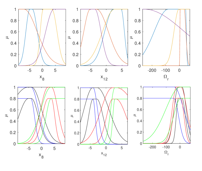
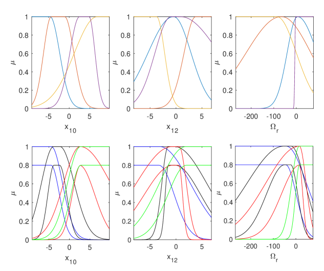
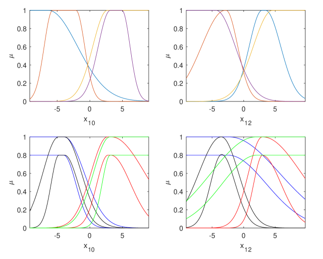
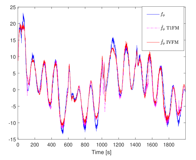
The validation of fuzzy models obtained (the fuzzy model type-2 ; IFVS and the fuzzy model type-1 ; T1FS) as shown in Fig. 8  9  10 and the Table 2 show that our proposed technique ( IVFM) is more close to real functions of system compared to the type-1 model.

Table 2: Comparison between RMSE of T1FM and IVFM

$f_{i}(x,\Omega)$	$\hat{f}_{i}(x,\theta_{fi})$	T1FM	IVFM
${f_{\phi}}(x,\Omega)$	${\hat{f}_{\phi}}({x_{8}},{x_{12}},{\theta_{f_{\phi}}})$	1.5958	1.4016
${f_{\theta}}(x,\Omega)$	${\hat{f}_{\theta}}({x_{10}},{x_{12}},{\theta_{f_{\theta}}})$	1.1717	1.1009
${f_{\psi}}(x,\Omega)$	${\hat{f}_{\psi}}({x_{10}},{x_{12}},{\theta_{f_{\psi}}})$	0.2072	0.1930

Figure 8: Comparaison between ${\hat{f}_{\phi}}({x})$ and ${f_{\phi}}({x})$

Figure 9: Comparaison between ${\hat{f}_{\theta}}({x})$ and ${f_{\theta}}({x})$

Figure 10: Comparaison between ${\hat{f}_{\psi}}({x})$ and ${f_{\psi}}({x})$

4 Indirect Adaptive control

The initial model of the antecedent part in Eqn. (4) plays an important role in the structure of the system. The previous clustering algorithm is used to build the initial structure of the unknown part of a nonlinear system with a fuzzy model. The laws of Lyapunov are then applied to adjust the identified model while maintaining system stability.

Let $\underline{e}(t)=\underline{x}_{m}(t)-\underline{x}(t)$ the error of tracking, $K=[k_{0},1]$ a vector of parameters of conception and the equation of sliding is given by:

$$\underline{e}_{s}(t)=\underline{e}+{k_{0}}\dot{\underline{e}}$$ (9)

where $e_{s}(t)=(e_{s_{x}},e_{s_{y}},e_{s_{z}},e_{s_{\theta}},e_{s_{\varphi}},e_{s_{\psi}})$ represent the sliding surface.

4.1 Design of fuzzy adaptive SMC control law

The approximed fonctions $f(x)$ and $g(x)$ with the universelle approximator flous, take the following forme:$\hat{f}(x,\theta)={\theta_{f}}^{T}{\varphi_{f}}(x)$ and $\hat{g}(x,\theta)={\theta_{g}}^{T}{\varphi_{g}}(x)$ With ${\varphi_{f}}$ and are the basis of fuzzy vector functions, supposed convenablement fixed by the fuzzy identification presented in  3.2, and are the vectors of paramètres ajustables supposed définis respectively in the domaine ${\Omega_{f}}$and ${\Omega_{g}}$ . We défine the sub-set ${S_{x}}\subseteq{\Re^{n}}$ as a space in which the trajectoiries of states $x$ stay inside it in the closed loop. The functions $f(x)$ and $g(x)$ are writen as follow :

$$\hat{f}(x,\theta_{f}) ={f^{*}}(x,\theta_{f}^{*})+w_{f}(x)\hfill$$ (10)

$$\hat{g}(x,\theta_{g}) ={g^{*}}(x,\theta_{g}^{*})+w_{g}(x)$$

with ${w_{f}}$ and ${w_{g}}$ represente errors of appriximation. ${f^{*}}(x,\,\theta)$ and ${g^{*}}(x,\,\theta)$ are respectivly the optimal parameters of $\hat{f}(x)$ and $\hat{g}(x)$ . The values of paramètres ${\theta_{f}}$ and ${\theta_{g}}$ minimise respectivly tthe errors of approximation ${w_{f}}(x)$ and ${w_{g}}(x)$ . those optimal paramètres satisfy :

$${\theta_{f}}^{*} =\arg\mathop{\min}\limits_{{\theta_{f}}\in{\Omega_{f}}}\left({{{\sup}_{x\in{S_{x}}}}\left|{{\theta_{f}}^{T}{\varphi_{f}}(x)-f(x)}\right|}\right)\hfill$$ (11)

$${\theta_{g}}^{*} =\arg\mathop{\min}\limits_{{\theta_{g}}\in{\Omega_{g}}}\left({{{\sup}_{x\in{S_{x}}}}\left|{{\theta_{g}}^{T}{\varphi_{g}}(x)-g(x)}\right|}\right)\hfill$$

We suppose that $\left|{{w_{f}}(x)}\right|\leq{W_{f}}$ and $\left|{{w_{g}}(x)}\right|\leq{W_{g}}$ where ${W_{f}}(x)$ and ${W_{g}}(x)$ are the known upper bound of approximation error. Both fonctions and can be choose arbitrairely small. The parametres of errors are :

$${\begin{array}[]{*{20}{c}}{{{\tilde{\theta}}_{f}}(t)={\theta_{f}}(t)-\theta_{f}^{*}}\\ {{{\tilde{\theta}}_{\beta}}(t)={\theta_{g}}(t)-\theta_{g}^{*}}\end{array}}$$ (12)

Considering the following proposed indirecte fuzzy control

Both terms ${u_{eq}}$ and ${u_{s}}$ will be calculated with details in the next sections. In the following we note IVFC (Interval value fuzzy control) and IVFM (Interval value fuzzy Model) for the control based on type-2 fuzzy system, in other hand we note T1FC and T1FM for the model based on type-1 fuzzy and Type-2 fuzzy system respectively.

4.1.1 Terme of equivalance control ${u_{eq}}$

take $\bar{e}_{s}(t)=k_{d-2}e^{\left({d-1}\right)}(t)+\cdot\cdot\cdot+{k_{0}}\dot{e}(t)$ in order to have ${\bar{e}_{s}}(t)={\dot{e}_{s}}(t)-{e^{\left(d\right)}}(t)$. The certainty equivalence control term Sastry and Isidori (1989) become as:

$$u_{eq}=-\frac{1}{\hat{g}(x)}(\hat{f}(x)+\nu(t))$$ (13)

where $\nu(t)={y_{d}}^{\left(d\right)}+\gamma{e_{s}}+{\bar{e}_{s}}$ and $\gamma>0$ is a design parameter. The dth derivative of the output error ${e^{\left(d\right)}}={y_{d}}^{\left(d\right)}-{y^{\left(d\right)}}$ with $u={u_{eq}}+{u_{s}}$, hence :

$$e^{(d)} =y_{d}^{(d)}-f(x)-g(x)u(t)$$ (14)

$$=y_{d}^{(d)}-f(x)-\frac{g(x)}{\hat{g}(x)}(-\hat{f}(x)+\nu(t))-(g(x))u_{s}$$

Note that the two first termes of the Eqn. (14):

$$y_{d}^{(d)}-f(x) =y_{d}^{(d)}-\hat{f}(x)-f(x)+\hat{f}(x)$$ (15)

$$=(-\hat{f}(x)+\nu(t))-f(x)+\hat{f}(x)-\gamma e_{s}-\bar{e}_{s}$$

We substitute Eqn. (15) in Eqn. (14), leads to :

$$e^{(d)} =\left({\hat{f}(x)-f(x)}\right)+\left({\hat{g}(x)-g(x)}\right)u_{eq}$$ (16)

$$-\gamma{e_{s}}-{\bar{e}_{s}}-g(x){u_{s}}$$

And with ${\bar{e}_{s}}={\dot{e}_{s}}-{e^{(d)}}$ , leads to :

$${\dot{e}_{s}}+\gamma{e_{s}}=\left({\hat{f}(x)-f(x)}\right)+\left({\hat{g}(x)-g(x)}\right){\text{ }}{u_{eq}}-\left({g(x)}\right){u_{s}}$$

4.1.2 law of parameters adaptation

Consider the lyapunov candidate function:

$$V_{i}=\frac{1}{2}e_{s}^{2}+\frac{1}{2\eta_{f}}{\tilde{\theta}_{f}}^{T}\tilde{\theta}_{f}+\frac{1}{2\eta_{g}}{\tilde{\theta}_{g}}^{T}\tilde{\theta}_{g}$$ (17)

Where ${\eta_{f}}>0$ and ${\eta_{g}}>0$ are the parameters of conception. The derivative of Lyapunov function Eqn. (17), gives us:

$$\dot{V}_{i} ={e_{s}}\left(-\gamma{e_{s}}+(\hat{f}-f)+\left(\hat{g}-g\right)u_{ce}-(g)u_{s}\right)$$ (18)

$$+\frac{1}{\eta_{f}}{\tilde{\theta}_{f}}^{T}{\dot{\tilde{\theta}}_{f}}+\frac{1}{\eta_{g}}{\tilde{\theta}_{g}}^{T}{\dot{\tilde{\theta}}_{g}}$$

In other hand ,

$$\hat{f}-f =\theta_{f}^{T}\phi_{f}(x)-{\theta^{*}_{f}}^{T}\phi_{f}(x)-{w_{f}}(x)$$ (19)

$$=\tilde{\theta}_{f}^{T}\phi_{f}(x)-w_{f}(x)\hfill$$

Same thing with $(\hat{g}-g)$ hence,

$${\dot{V}_{i}} =+\left({{{\tilde{\theta}}_{f}}^{T}{\phi_{f}}-{w_{f}}+{{\tilde{\theta}}_{g}}^{T}{\phi_{g}}{u_{eq}}-w_{g}{u_{ce}}-g{u_{s}}}\right){e_{s}}$$ (20)

$$+\frac{1}{\eta_{f}}{\tilde{\theta}_{f}}^{T}{\dot{\tilde{\theta}}_{f}}+\frac{1}{\eta_{g}}{\tilde{\theta}_{g}}^{T}\dot{\tilde{\theta}}_{g}-\gamma{e_{s}}^{2}$$

We choose the following adaptation laws :

$$\dot{\theta}_{f}(t) =-{\eta_{f}}{\varphi_{f}}(x)e_{s}\hfill$$ (21)

$$\dot{\theta}_{g}(t) =-{\eta_{g}}{\varphi_{g}}(x)e_{s}u_{eq}\hfill$$

where ${\varphi_{f}}(x)=\tfrac{1}{2}\left({{\xi_{l}}^{f}+{\xi_{r}}^{f}}\right)$ and ${\varphi_{g}}(x)=\tfrac{1}{2}\left({{\xi_{l}}^{g}+{\xi_{r}}^{g}}\right)$ , the speed of adaptation related to the choice of the values of ${\eta_{f}}$ and ${\eta_{g}}$ . we suppose that the ideal parameters are constants ${\dot{\tilde{\theta}}_{f}}={\dot{\theta}_{f}}$ and ${\dot{\tilde{\theta}}_{g}}={\dot{\theta}_{g}}$. With those conditions we find that:$\frac{1}{{{\eta_{g}}}}{\tilde{\theta}_{g}}^{T}{\dot{\tilde{\theta}}_{g}}=-{\tilde{\theta}_{g}}^{T}{\varphi_{g}}\left(x\right){e_{s}}{u_{eq}}$ and $\frac{1}{{{\eta_{f}}}}{\tilde{\theta}_{f}}^{T}{\dot{\tilde{\theta}}_{f}}=-{\tilde{\theta}_{f}}^{T}{\varphi_{f}}\left(x\right){e_{s}}$ hence,

$${\dot{V}_{i}}=-\gamma{e_{s}}^{2}+\left({-{w_{f}}(x)-{w_{g}}(x){u_{eq}}-g(x){u_{s}}}\right){e_{s}}$$ (22)

4.1.3 Projection Modification to Parameter’s Update Laws

The laws of adaptation in the equations (18-19) don’t garanty that ${\theta_{f}}\in\,{\Omega_{f}}$ and ${\theta_{g}}\in\,{\Omega_{g}}$ . We must use the projection to insure that (e.g. to guaranty that $\hat{g}\left(x\right)\geq{g_{0}}$ ). We suppose in particuliar that the i^th component of ${\theta_{f}}^{*}$ and ${\theta_{f}}^{*}$ is in the known intervalle: $\theta_{{f_{i}}}^{*}\in{\text{[}}{\theta_{{f_{i}}}}^{\text{min}},{\theta_{f_{i}}}^{\text{max}}{\text{]}}$ and $\theta_{{g_{i}}}^{*}\in{\text{[}}\theta_{{g_{i}}}^{{\text{min}}},\theta_{{g_{i}}}^{{\text{max}}}{\text{]}}$ and we want that and , we define as a point in the acceptable region. We can resume this algorithm by using the following rule : $\text{if }{\theta_{f}}(t)\notin\,[{\theta_{f}}^{\min},{\theta_{f}}^{\max}]$ and $\theta_{f}^{ud}({\theta_{f}}-\theta_{f}^{m})\geq 0$ then ${\dot{\theta}_{f}}(t)=0$ else $\dot{\theta}_{f}(t)=-{\eta_{f}}{\varphi_{f}}e_{\text{s}}u_{\text{eq}}$
In the stability analysis, this projection modification to the update laws will always result in a parameter estimation error that will decrease ${V_{i}}$ at least as much as if the projection were not used; hence, the right-hand side of Eqn. (22) will overbound the ${\dot{V}_{i}}$ that would result if projection is used. For this reason, we conclude that:

$${\dot{V}_{i}}\leq-\gamma{e_{s}}^{2}\,+\left({-{w_{f}}(x)-{w_{g}}(x){u_{ce}}-g(x){u_{s}}}\right){e_{s}}$$ (23)

4.1.4 Sliding Mode Control Term

To ensure that Equation Eqn. (23) is less than or equal to zero, we choose:

$${u_{s}}=\eta(x)\operatorname{sgn}({e_{s}})=\frac{1}{g_{0}}\left({{W_{f}}(x)+{W_{g}}(x)\left|u_{eq}\right|}\right)\operatorname{sgn}(e_{s})$$

We see that : $-(w_{f}(x)+w_{g}(x)u_{ce}){e_{s}}\leq({|w_{f}(x)|+|w_{g}(x)u_{ce}|})|e_{s}|$ with $\frac{g(x)}{g_{0}}\geq 1$ hence:

$$\dot{V}_{i} \leq-\gamma e_{s}^{2}+(|{w_{f}}(x)|+|{w_{g}}(x)u_{eq}|)|e_{s}|$$ (24)

$$-{e_{s}}\frac{g}{g_{0}}(W_{f}(x)+W_{g}(x)|u_{eq}|)\operatorname{sgn}(e_{s})$$

$${\dot{V}_{i}} \leq-\gamma{e_{s}}^{2}+\left|{{w_{f}}\left(x\right)\left|{\left|{e_{s}}\right|}+\right|{w_{g}}\left(x\right){u_{eq}}}\right|\left|{e_{s}}\right|$$ (25)

$$-{e_{s}}sgn\left({e_{s}}\right){W_{f}}\left(x\right)-{e_{s}}sgn\left({e_{s}}\right){W_{g}}\left(x\right)\left|u_{eq}\right|$$

where $|e_{s}|=e_{s}sgn(e_{s})$ ,$\forall{e_{s}}\neq 0:$ and $|w_{g}(x)|\leq W_{g}(x)$ then :

$$|{w_{f}}(x)||e_{s}|-{e_{s}}sgn({e_{s}}){W_{f}}(x)=|e_{s}|(|w_{f}(x)|-W_{f}(x))\leq 0$$

$$\left|{{w_{g}}(x){u_{eq}}}\right|\left|{{e_{s}}}\right| -{e_{s}}sgn({e_{s}}){W_{g}}(x)\left|{{u_{eq}}}\right|=$$

$$\left|{{e_{s}}}\right|(\left|{{w_{g}}(x){u_{eq}}}\right|-{W_{g}}(x)\left|{{u_{eq}}}\right|)\leq 0$$

$$\dot{V}_{i}\leq-\gamma{e_{s}}^{2}$$ (26)

because $\gamma{e_{s}}^{2}\geq 0$ , this show that ${\dot{V}_{i}}$ which is a measure of the tracking error and parameter estimation error, is a nonincreasing function of time. Notice that $\gamma>0$ has an influence on how fast $V_{i}\mapsto 0$. By picking $\gamma$ larger you will often get faster convergence of the tracking error.

4.1.5 Asymptotic Convergence of the Tracking Error and Boundedness of Signals

Due the hypothysis considered (that the reference signals are bounded, $x$ is measurable, $d=n$, and the projection ensures that the ${u_{eq}}$ term is well-defined), the following statements hold:

1. The system output $y,\dot{y},...,{y^{(d-1)}}$ are bounded

2. The control signal $u$, ${u_{eq}}$ et ${u_{s}}$ are bounded.

3. The parameteres ${\theta_{g}}(t)$ and ${\theta_{g}}(t)$ are bounded.

4. The magnitude of the output error decreases at least asymptotically to zero ( $\mathop{\lim}\limits_{t\to\infty}e(t)=0$)

To prove this, Note that since $V_{i}$ is positive and ${\dot{V}_{i}}\leq-\gamma{e_{s}}^{2}$ . We know that ${e_{s}},{\theta_{f}}$ and ${\theta_{g}}$ are bounded. since $e_{s}$ is bounded and $y_{r}$ and its derevatives are bounded. We know that $y,\dot{y},...,{y^{(d-1)}}$ are bounded. Hence, $x$ are bounded. Hence, $f(x),\hat{f}(x),g(x)$ and $\hat{g}(x)$ are bounded. Since $x$ is bounded and $\hat{g}(x)\geq{g_{0}}$ , $u_{eq}$ and $u_{s}$ and hence $u$, are bounded. Next, note that :

$$\int\limits_{0}^{\infty}{\gamma e_{s}^{2}dt}\leq-{\int V_{i}}dt={V_{i}}(0)-{V_{i}}(\infty)$$ (27)

This establishes that ${e_{s}}\in{L_{2}}{\text{ ou }}{L_{2}}=\left\{{z(t):\int_{0}^{\infty}{{z^{2}}(t)}dt<\infty}\right\}$ since ${V_{i}}\left(0\right)$ and ${V_{i}}\left(\infty\right)$ are bounded. Note that via the equation (15), ${\dot{e}_{s}}$ is bounded. Hence, because ${\dot{e}_{s}}$ and ${e_{s}}$ are bounded and ${e_{s}}\in{L_{2}}$ , and via the barbarat’s lemma we have $\mathop{\lim}\limits_{t\to\infty}{e_{s}}(t)=0$ . Hence $\mathop{\lim}\limits_{t\to\infty}e(t)=0$.
It is possible to reduce the chattering that can be result in the sliding mode term of control, we introduce ${{\mathbf{e}}_{\varepsilon}}=(e_{\varepsilon_{x}},e_{\varepsilon_{y}},e_{\varepsilon_{z}},e_{\varepsilon_{\theta}},e_{\varepsilon_{\varphi}},e_{\varepsilon_{\psi}})$ we can use the smooth function $\textnormal{sgn}({e_{s}})$ Slotine and Coetsee (1986). In this case, however, you only get convergence to an neighborhood of ${e_{s}}=0$ . To prove the stability, we define the error ${e_{\varepsilon}}$.

$${e_{\varepsilon}}={e_{s}}-\varepsilon{sat}(\frac{e_{s}}{\varepsilon})$$ (28)

where

$${sat(x)}=\left\{\begin{array}[]{*{20}{c}}1{\textnormal{ si}}\,\,1\leq x\hfill\\ x{\textnormal{ si}}\,\,-1<x<1\hfill\\ -1{\textnormal{ si}}\,\,x\leq-1\hfill\end{array}\right.$$

where ${e_{\varepsilon}}$ represent the distance between ${e_{s}}$ and the desired “boundary layer,”, so the ${e_{\varepsilon}}=0$ when ${e_{s}}$ is inside the layer. The equivalent control is defined to be:

$${u_{eq}}=-\tfrac{1}{\hat{g}(x)}(\hat{f}(x)+{\nu_{\varepsilon}}(t))\,\,{\text{with}}\,\,{\nu_{\varepsilon}}(t)={y_{d}}^{(n)}+\gamma{e_{\varepsilon}}+{\bar{e}_{s}}$$

we consider the following lyapunouv function:

$${V_{i}}=\frac{1}{2}{e_{\varepsilon}}^{2}+\frac{1}{{2{\eta_{f}}}}{\tilde{\theta}_{f}}^{T}{\tilde{\theta}_{f}}+\frac{1}{{2{\eta_{g}}}}{\tilde{\theta}_{g}}^{T}{\tilde{\theta}_{g}}$$

And the Adaptation laws became :

$${\dot{\theta}}_{f}(t) =-{\eta_{f}}{\varphi_{f}}(x){e_{\varepsilon}}$$ (29)

$${\dot{\theta}}_{g}(t) =-{\eta_{g}}{\varphi_{g}}(x){e_{\varepsilon}}{u_{eq}}$$

with those laws the derived lyapunov functions:

$${\dot{V}_{i}}\leq-\gamma{e_{\varepsilon}}^{2}\,+\left({\left|{{w_{f}}(x)}\right|+\left|{{w_{g}}(x){u_{ce}}}\right|}\right)\left|{{e_{\varepsilon}}}\right|-g(x){u_{s}}{e_{\varepsilon}}$$

the terme $u_{s}$ in Eqn. (30) become a control with smooth action.

$${u_{s}}=\frac{1}{{{g_{0}}}}\left({{W_{f}}(x)+{W_{g}}(x)\left|{{u_{eq}}}\right|}\right){\text{sat}}(\frac{{{e_{s}}}}{\varepsilon})$$ (30)

with ${e_{\varepsilon}}{\text{sat}}(\frac{e_{s}}{\varepsilon})=\left|e_{\varepsilon}\right|$, we can proof that $\dot{V}_{i}\leq-\gamma{e_{\varepsilon}}^{2}$ , that’s make $\left|{{e_{\varepsilon}}}\right|$ asymptotically stable , in addition ${e_{s}}$ will converge to the $\varepsilon$-neighbor of $e_{s}=0$, and $e$ will converge to 0.

4.2 Control of position and attitude of Quadrotor

Proposition 1: for the conception of attitude controller described by the following sub-systems  (6), (7) and  (8).

we propose a sliding mode controller for every subsystem $i$ where $i=\left\{\phi,\theta,\psi\right\}\,$ as follow:

$${U_{i}}={u_{eq_{i}}}+{u_{s_{i}}}$$ (31)

where :

$${u_{e{q_{i}}}} =-\frac{1}{{{{\hat{g}}_{i}}(x)}}\left({{{\hat{f}}_{i}}(x,{\theta_{{f_{i}}}})+\ddot{y}_{{d_{i}}}+\gamma{e_{{\varepsilon_{i}}}}+{{\bar{e}}_{{s_{i}}}}}\right)$$

$${u_{{s_{i}}}} =\frac{1}{g_{0i}}\left({{W_{{f_{i}}}}(x)+{W_{{g_{i}}}}(x)|u_{e{q_{i}}}|}\right)sat(\frac{e_{s_{i}}}{\varepsilon})$$

where ${\bar{e}_{s}}={k_{i}}e$ , ${y_{{d_{i}}}}=\left\{{{\phi_{d}},{\varphi_{d}},{\theta_{d}}}\right\}\,$, $d=2$ ,$W_{f_{i}}(x)$ and $W_{g_{i}}(x)$ are the errors bounds of the approximation of $f_{i}$ and $g_{i}$ respectively. with $g_{0_{i}}$ is the minimum value of $b_{i}$ . the control input Eqn. (31) ensures the asymptotic convergence of $\phi,\theta$ and $\psi$ to ${\phi_{d}},{\theta_{d}},\,{\psi_{d}}$ respectively.

Proof : similarly, to sections  4.1.1 and  4.1.4 , we take $n=2$, the equations Eqn. (13) and Eqn. (30) became:

$${U_{i}}=\frac{1}{{\hat{b}}_{i}}\left(-{{\hat{f}}_{i}}\left(x,\varphi_{f_{i}}\right)+\gamma{e_{\varepsilon i}}+{{\bar{e}}_{si}}+\ddot{y}_{i_{d}}\right)\\ +{\frac{1}{g_{0{i}}}(W_{f_{\phi}}(x)+W_{g_{i}}(x)|u_{e{q_{i}}}|)}{\text{sat}}(\frac{e_{s\phi}}{\varepsilon})$$ (32)

using the equations in Eqn. (29), the adaptations laws can be written as follow:

$${\dot{\theta}}_{f{i}} =-{\eta_{f_{i}}}{\varphi_{f_{i}}}\left({{x}}\right){e_{\varepsilon_{i}}}\hfill$$ (33)

$${\dot{\theta}}_{g{i}} =-{\eta_{g_{i}}}{e_{\varepsilon i}}u_{eq_{i}}\hfill$$

Notice that the functions $g_{i}$ in Eqn. (33) is considered as a constants that’s why it is approximated with a constant and not a fuzzy function, so we take ${\varphi_{f_{i}}}=1$ .

Proposition 2 : for the altitude controller, the subsystem that governs the movement $z(t)$ is :

$$\left({\begin{array}[]{*{20}{c}}{{{\dot{x}}_{7}}}\\ {{{\dot{x}}_{8}}}\end{array}}\right)=\left({\begin{array}[]{*{20}{c}}{\dot{z}}\\ {{f_{z}}-U{g_{z}}{U_{z}}}\end{array}}\right)\,$$

where $U=(\cos\phi\cos\theta)$ , ${g_{z}}=\frac{1}{m}$ and ${f_{z}}$ is the gravity $g$. The sliding mode control Eqn. (34) ensure the convergence of $z(t)$ toward the consign $z_{d}$

$${U_{z}}=\frac{1}{{U{g_{z}}}}(-{\hat{f}_{z}}(x)+{\ddot{z}_{d}}+\gamma{e_{\varepsilon z}}+{\bar{e}_{sz}})\\ +\frac{1}{g_{0}}\left({{W_{f_{z}}}(x)/(U)+{W_{g_{z}}}(x)\left|{u_{eq_{z}}}\right|}\right){\text{sat}}(\frac{e_{sz}}{\varepsilon})$$ (34)

Where ${W_{f_{z}}}(x)$ and ${W_{g_{z}}}(x)$ are the bounded limit of error of the approximation of ${f_{z}}$ and ${g_{z}}$ respectively
Proof : following the same procedure in the sections  4.1.1 and  4.1.4, considering ${\ddot{z}}={f_{4}}\left(x\right)-Ug_{z}{U_{z}}(t)$ where , the term of equivalent control is defined as :

$${u_{e{q_{z}}}}=-\tfrac{1}{U{g_{z}}}\left({{{\hat{f}}_{z}}(x|{\theta_{f_{z}}})+{{\ddot{z}}_{d}}+\gamma{e_{\varepsilon_{z}}}+{{\bar{e}}_{s_{z}}}}\right)$$

where $\nu(t)={\ddot{z}_{d}}+\gamma e_{s_{z}}+{\bar{e}_{s_{z}}}$ and $\gamma>0$

The 2^end derivative of the output error, along with the equation Eqn. (14) we can write:

$$\ddot{e}={\ddot{z}_{d}}-{f_{z}}(x)-\tfrac{g_{z}}{{\hat{g}}_{z}}\left(-{{\hat{f}}_{z}}(x)+\nu(t)\right)-U{g_{z}}{u_{s}}$$ (35)

Take the two first terms as follow:

$${\ddot{z}_{d}}-{f_{z}}(x)=\left(-{{\hat{f}}_{z}}(x)+\nu(t)\right)-{f_{z}}(x)+{\hat{f}_{z}}(x)-\gamma{e_{{s_{z}}}}-{\bar{e}_{{s_{z}}}}$$

we substitute both terms in the equation Eqn. (35), using ${\bar{e}_{s}}={\dot{e}_{s}}-{e^{(d)}}$ we find:

$${\dot{e}_{s}}+\gamma{e_{s}}=(\hat{f}_{z}-f_{z})+(\hat{g}_{z}-g_{z})U{u_{eq_{z}}}-Ug{u_{s}}$$

The candidate function of Lyapunov ${V_{i}}$ :

$${V_{z}}=\frac{1}{2}{e_{{\varepsilon_{z}}}}^{2}+\frac{1}{{2{\eta_{f}}}}{\tilde{\theta}_{{f_{z}}}}^{T}{\tilde{\theta}_{{f_{z}}}}+\frac{1}{{2{\eta_{g}}}}{\tilde{\theta}_{{g_{z}}}}^{T}{\tilde{\theta}_{{g_{z}}}}$$

where ${\eta_{f}}>0$ and ${\eta_{f}}>0$ are the adaptation gain. the derivative of $V_{i}$ gives us:

$$\dot{V}_{z} =({{{\tilde{\theta}}_{f_{z}}}^{T}{\phi_{f}}-{w_{f_{z}}}+U{{\tilde{\theta}}_{g_{z}}}^{T}{\phi_{g}}u_{eq_{z}}-U{w_{g}}{u_{eq_{z}}}-Ug{u_{s}}})e_{\varepsilon_{z}}$$ (36)

$$-\gamma e_{{\varepsilon_{z}}}^{2}+\frac{1}{{{\eta_{f}}}}{\tilde{\theta}_{f}}^{T}{\dot{\tilde{\theta}}_{f}}+\frac{1}{{{\eta_{g}}}}{\tilde{\theta}_{g}}^{T}{\dot{\tilde{\theta}}_{g}}$$

Suppose that those ideal parameters are constants ${\dot{\tilde{\theta}}_{f}}={\dot{\theta}_{f}}$ and ${\dot{\tilde{\theta}}_{g}}={\dot{\theta}_{g}}$, and the chosen adaptation law is:

$$\begin{array}[]{*{20}{l}}{{\dot{\theta}}_{f_{z}}}\left(t\right)=-{\eta_{f_{z}}}{\varphi_{{f_{z}}}}\left(x\right){e_{{\varepsilon_{z}}}}\\ {{\dot{\theta}}_{g_{z}}}\left(t\right)=-{\eta_{g_{z}}}{\varphi_{{g_{z}}}}\left(x\right){e_{{\varepsilon_{z}}}}{u_{e{q_{z}}}}{\text{(}}\cos\phi\cos\theta)\end{array}$$

That’s lead to: $\frac{1}{\eta_{g}}{\tilde{\theta}_{g}}^{T}{\dot{\tilde{\theta}}_{g}}=-{\tilde{\theta}_{g}}^{T}{\varphi_{g}}\left(x\right){e_{{\varepsilon_{z}}}}{u_{eq}}$ and $\tfrac{1}{{{\eta_{f}}}}{\tilde{\theta}_{f}}^{T}{\dot{\tilde{\theta}}_{f}}=-{\tilde{\theta}_{f}}^{T}{\varphi_{f}}\left(x\right){e_{\varepsilon_{z}}}$ , so the equation Eqn. (36) can be written as:

$${\dot{V}_{z}}=-\gamma{e_{\varepsilon_{z}}}^{2}+\left({-{w_{f}}(x)-U{w_{g}}(x){u_{eq_{z}}}-U{g(x)}{u_{s}}}\right){e_{{\varepsilon_{z}}}}\,$$

To analyze the stability, we conclude that:

$${\dot{V}_{z}}\leq-\gamma{e_{{\varepsilon_{z}}}}^{2}+\left({-{w_{f_{z}}}(x)-U{w_{g_{z}}}(x){u_{eq_{z}}}-U{g(x)}{u_{s}}}\right){e_{{\varepsilon_{z}}}}$$ (37)

To ensure that the equation Eqn. (37) must be less than or equal to zero, we choose:

$${u_{s}}=\tfrac{1}{g_{0}}\left(\tfrac{{W_{f_{z}}}(x)}{U_{1}}+{W_{g_{z}}}(x)\left|{{u_{eq_{z}}}}\right|\right){\text{sat}}(\tfrac{{{e_{s}}}}{\varepsilon})=\eta(x){\text{sat}}(\tfrac{e_{s}}{\varepsilon})$$

We note that: $-\left({{w_{f}}(x)+{w_{g}}(x){u_{eq}}}\right){e_{s}}\leq\left({\left|{{w_{f}}(x)}\right|+\left|{{w_{g}}(x){u_{eq}}}\right|}\right)\left|{{e_{s}}}\right|$ , so:

$$\dot{V}_{z}=-\gamma{e_{s}}^{2}+(-{w_{f_{z}}}(x)-U{w_{g_{z}}}(x){u_{eq_{z}}}\\ {-U\tfrac{g_{z}}{g_{0_{z}}}(\tfrac{W_{f_{z}}(x)}{U}+{W_{g_{z}}}(x)|u_{eq_{z}}|})\text{sat}(\tfrac{e_{s}}{\varepsilon}))e_{\varepsilon}$$ (38)

$${\dot{V}_{z}} \leq-\gamma e_{{\varepsilon_{z}}}^{2}+\left({\left|{{w_{f_{z}}}(x)}\right|+\left|{U{w_{g_{z}}}(x){u_{eq_{z}}}}\right|}\right)\left|{e_{\varepsilon_{z}}}\right|$$ (39)

$$-U{e_{{\varepsilon_{z}}}}g_{z}(x)({\tfrac{1}{g_{0_{z}}}\left({\tfrac{{W_{f_{z}}}(x)}{U}+{W_{g}}(x)\left|{{u_{eq_{z}}}}\right|}\right){\text{sat}}(\tfrac{e_{s}}{\varepsilon})})$$

Now, we consider the last term of the equation Eqn. (39) and because $\tfrac{{g_{z}(x)}}{g_{0_{z}}}\geq 1$ so :

$$\dot{V_{i}} =-\gamma{e_{\varepsilon_{z}}}^{2}+|{{w_{f_{z}}}(x)||{e_{s}}|-{e_{\varepsilon}}sat(\tfrac{e_{\varepsilon}}{\varepsilon}){W_{f_{z}}}(x)}$$ (40)

$$+|U{w_{g_{z}}}(x)u_{eq_{z}}||{e_{\varepsilon}}|-U{e_{\varepsilon}}sat(\tfrac{e_{\varepsilon}}{\varepsilon}){W_{g_{z}}}(x)|{u_{eq_{z}}}|$$

with $|{e_{\varepsilon}}|={e_{s}}sat({e_{s}}/\varepsilon)$ , $|{w_{f}}(x)|\leq{W_{f}}(x)$ and $|{w_{g}}(x)|\leq{W_{g}}(x)$ so:

$$|{w_{f_{z}}}(x)||{e_{\varepsilon}}| -{e_{\varepsilon}}sat(\frac{e_{s}}{\varepsilon}){W_{f}}\left(x\right)$$ (41)

$$=\left|{{e_{\varepsilon}}}\right|\left({\left|{{w_{f_{z}}}\left(x\right)}\right|-{W_{f_{z}}}\left(x\right)}\right)\leq 0$$

$$|U{w_{g_{z}}}(x){u_{eq_{z}}}||{e_{\varepsilon}}|-U{e_{\varepsilon}}{\text{sat}}(\tfrac{e_{s}}{\varepsilon}){W_{g_{z}}}(x)|u_{eq_{z}}|=\\ \left\{\begin{array}[]{l l}&U\left|{e_{\varepsilon}}\right|\,\left({\left|{{w_{g_{z}}}{u_{eq_{z}}}}\right|-{W_{g_{z}}}\left|{u_{eq_{z}}}\right|}\right)\leq 0{\text{ if}}\,\,U\geq 0\\ &\left|U\right|\left|{{e_{\varepsilon}}}\right|\,\left({\left|{{w_{g_{z}}}{u_{eq_{z}}}}\right|+{W_{g_{z}}}\left|{u_{eq_{z}}}\right|}\right)\leq 0{\text{ if}}\,\,U<0\\ \end{array}\right.$$ (42)

$${\dot{V}_{z}}=-\gamma{e_{\varepsilon}}^{2}+\left|{e_{\varepsilon}}\right|\left({\left|{{w_{f_{z}}}\left(x\right)}\right|-{W_{f_{z}}}\left(x\right)}\right)\\ +\left|{u_{eq_{z}}}\right|\left|{e_{\varepsilon}}\right|\left({\left|{U{w_{g_{z}}}(x)}\right|-U{W_{g_{z}}}(x)}\right)$$ (43)

Since $\gamma{e_{\varepsilon}}^{2}\geq 0$ this shows that ${V_{z}}$ is a non-increasing function of time.

Proposition 3 : from the Eqn. (5), the subsystems that govern the dynamics of position $(x,y)$ is given by:

$$\left({\begin{array}[]{*{20}{c}}{{\dot{x}}_{9}}\\ {{\dot{x}}_{10}}\end{array}}\right)=\left({\begin{array}[]{*{20}{c}}{\dot{x}}\\ {{u_{x}}\tfrac{1}{m}{U_{z}}}\end{array}}\right)$$ (44)

$$\left({\begin{array}[]{*{20}{c}}{\dot{x}}_{11}\\ {\dot{x}}_{12}\end{array}}\right)=\left({\begin{array}[]{*{20}{c}}{\dot{y}}\\ {{u_{y}}\tfrac{1}{m}{U_{z}}}\end{array}}\right)$$ (45)

The following proposed indirect fuzzy adaptative control $u_{x}$ and $u_{y}$ Eqn. (46):

$${u_{x}} =\frac{\hat{m}}{U_{z}}({x_{d}}^{\left(n\right)}+\gamma{e_{\varepsilon_{x}}}+{{\bar{e}}_{sx}})+{\eta_{x}}(x){\text{sat}}(\tfrac{e_{s_{x}}}{\varepsilon})\hfill$$ (46)

$$\,{u_{y}} =\frac{\hat{m}}{U_{z}}({y_{d}}^{\left(n\right)}+\gamma{e_{\varepsilon_{y}}}+{{\bar{e}}_{sy}})+{\eta_{y}}(x){\text{sat}}(\tfrac{e_{s_{y}}}{\varepsilon})\hfill$$

Ensure the stability toward the desired trajectory asymptotically.

Where ${\eta_{x}}(x)=\tfrac{1}{g_{05}}\left({+{W_{g_{5}}}(x)\left|{{u_{eq}}}\right|}\right)$ and ${\eta_{y}}(x)=\tfrac{1}{{{g_{06}}}}\left({+{W_{g_{6}}}(x)\left|{{u_{eq}}}\right|}\right)$ with ${W_{g_{5}}}(x)$ and ${W_{g_{6}}}(x)$ are the known bounds of approximation errors of functions: ${g_{5}}$ and ${g_{6}}$ respectively.

proof : for the subsystem that govern the variable $x$, we have : $\hat{g}=\frac{1}{m}\to{u_{x}}\frac{1}{m}{U_{1}}={u_{x}}{\hat{g}_{x}}{U_{z}}$ and by the choice of the candidate function of Lyapunov ${V_{i}}$ where $i=\left\{x,y\right\}\,$ :

$${V_{i}}=\frac{1}{2}{e_{{\varepsilon_{i}}}}^{2}+\frac{1}{{2{\eta_{f}}}}{\tilde{\theta}_{{f_{i}}}}^{T}{\tilde{\theta}_{{f_{i}}}}+\frac{1}{{2{\eta_{g}}}}{\tilde{\theta}_{{g_{i}}}}^{T}{\tilde{\theta}_{{g_{i}}}}$$

its derivative is given by :

$${\dot{V}_{i}} =\left({{U_{z}}{{\tilde{\theta}}_{g}}^{T}{\phi_{g}}{x}{u_{eq_{i}}}-{U_{z}}{w_{g}}(x){u_{eq_{i}}}-{U_{1}}\left({g_{x}}\right){u_{s_{i}}}}\right){e_{\varepsilon}}$$ (47)

$$+\frac{1}{\eta_{g}}{\tilde{\theta}_{g}}^{T}{\dot{\tilde{\theta}}_{g}}-\gamma{e_{\varepsilon}}^{2}\,$$

We take the following adaptation law: ${\dot{\theta}_{g}}\left(t\right)=-{\eta_{g}}{\varphi_{g}}\left(x\right){e_{{\varepsilon_{x}}}}{u_{eq}}{U_{z}}$

If the parameter $g_{i}$ is constant, so the adaptation law for the position controller is : ${\dot{\theta}_{g}}\left(t\right)=-{\eta_{g}}{e_{{\varepsilon_{x}}}}{u_{eq_{i}}}{U_{z}}$

$${\dot{V}_{i}} =\left({{U_{z}}{{\tilde{\theta}}_{g}}^{T}{\phi_{g}}{\text{(}}x{\text{)}}{u_{eq_{i}}}-{U_{1}}{w_{g}}(x){u_{eq_{i}}}-{U_{z}}\left({g(x)}\right){u_{s}}}\right){e_{s}}$$ (48)

$$-\gamma{e_{\varepsilon}}^{2}-{U_{z}}{\tilde{\theta}_{g}}^{T}{\varphi_{g}}\left(x\right){e_{\varepsilon}}{u_{{eq_{i}}}}$$

$$\Rightarrow{\dot{V}_{i}}\leq-\gamma{e_{\varepsilon}}^{2}\,+\left({-{U_{z}}{w_{g}}(x){u_{eq_{i}}}-{U_{z}}\left({{g_{x}}}\right){u_{s_{i}}}}\right){e_{\varepsilon}}$$

To ensure that the equation Eqn. (48) being less or equal to zero, we choose ${u_{s}}$ as follow:

$${u_{{s_{x}}}}=\tfrac{g_{i}}{g_{0_{i}}}\left({{W_{g_{i}}}(x)\left|{{u_{eq_{i}}}}\right|}\right){\text{sat}}(\frac{{{e_{{s_{x}}}}}}{\varepsilon})$$

We constate that : $-\left({+{w_{g}}(x){u_{eq_{i}}}}\right){e_{\varepsilon}}\leq\left({+\left|{{w_{g}}(x){u_{eq_{i}}}}\right|}\right)\left|{{e_{\varepsilon}}}\right|$ so :

$${\dot{V}_{i}}=\left(-{U_{1}}{w_{g}}(x){u_{eq_{i}}}-{U_{z}}\left(\tfrac{g_{i}}{{g_{0}}_{i}}\right)\left({{W_{g_{5}}}(x)|{u_{eq_{i}}}|}\right){\text{sat}}({e_{s}}/\varepsilon)\right){e_{\varepsilon}}\\ -\gamma{e_{\varepsilon}}^{2}+\\$$

$${\dot{V}_{i}} \leq-\gamma e_{\varepsilon}^{2}+(|{{U_{z}}{w_{g}}(x)u_{eq_{i}}}|)|{e_{\varepsilon}}|$$ (49)

$$-{U_{z}}{e_{\varepsilon}}\left({\tfrac{g_{i}}{{g_{0}}_{i}}\left({{W_{g_{i}}}(x)\left|{{u_{eq_{i}}}}\right|}\right){\text{sat}}(\frac{e_{s}}{\varepsilon})}\right)$$

With : $(\tfrac{g_{i}}{g_{0_{i}}})\geq 1$ ,${U_{z}}\geq 0$ , $|{w_{f_{i}}}(x)|\leq{W_{f_{i}}}{(x)}$ and $|w_{g_{i}}(x)|\leq{W_{g_{i}}}(x)$ then $\forall{e_{s}}\neq 0$ we have

$${\dot{V}_{i}}=$$ (50)

$$-\gamma{e_{\varepsilon}}^{2}+\left|{{U_{z}}{w_{g_{i}}}(x){u_{eq_{i}}}}\right|\left|{{e_{\varepsilon}}}\right|-{U_{z}}{e_{\varepsilon}}{\text{sat}}(\tfrac{e_{s}}{\varepsilon}){W_{g_{i}}}(x)\left|{u_{eq_{i}}}\right|$$

$$={U_{z}}\left|{{e_{\varepsilon}}}\right|(\left|{w_{g_{i}}(x){u_{eq_{i}}}}\right|-{W_{g_{i}}}(x)\left|{u_{eq_{i}}}\right|)\leq 0$$

$${\dot{V}_{i}} \leq-\gamma{e_{\varepsilon}}^{2}$$

since $\gamma{e_{\varepsilon}}^{2}\geq 0$ , this shows that $V_{i}$, is a nonincreasing function of time.

The correspondent’s angles are given by the two following equations Eqn. (51):

$$\begin{gathered}{\phi_{d}}=\arcsin({u_{x}}\sin{\psi_{d}}-{u_{y}}\cos{\psi_{d}})\hfill\\ {\theta_{d}}=\arcsin(\frac{1}{{\cos\phi}}({u_{x}}\cos{\psi_{d}}-{u_{y}}\sin{\psi_{d}}))\hfill\\ \end{gathered}$$ (51)

for $\psi\cong 0$ we can approximate the Eqn. (51) using the following approximations: $\cos{\psi_{d}}\approx 1\,\textnormal{and}\,\sin{\psi_{d}}\approx 0\Rightarrow{\phi_{d}}=\arcsin(-{u_{y}})$ and ${\theta_{d}}=\arcsin(\frac{1}{{\cos\phi}}{u_{x}})$

5 Results and discussions

To verify the reliability and robustness of the controller with simulations of tracking in the presence of different disturbance levels, considering the results obtained using the proposed control in Section  4.2 and considering the various trajectories where we use a sampling step of $0.01$ and ${W_{{f_{i}}}}=0.1\,$ for $i=\left\{{\phi,\theta,\psi}\right\}$ and ${W_{g_{j}}}=0.1$ for $\,j=\left\{{\phi,\theta,...,y,z}\right\}$ and $\gamma=10$ for attitude and altitude control, while $\gamma=2$ and $K=[5,1]$ for position control.

5.1 Simulation with Disturbance

5.1.1 Attitude Control:

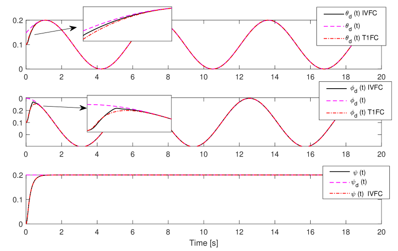
this test is about applying our proposed control to quadrotor to study its behavior in addition to its performances. Take the following trajectory:

$$\left\{\begin{gathered}\,{\theta_{d}}(t)=sin(t)\,;{\varphi_{d}}(t)=sin(t+\pi)\,\,\,\,\hfill\\ {\psi_{d}}(t)=0.2\,\,\,\,\,\,{z_{d}}(t)=1\,\,\,\,\,\hfill\\ \end{gathered}\right.\forall t$$

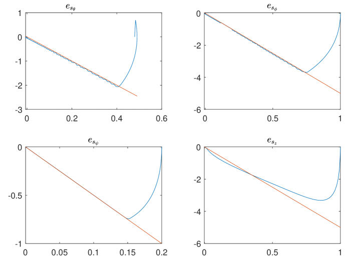
The desired and the real angles of output (in radians) are presented in Fig. 11, and the sliding errors are presented in Fig. 12.

Figure 11: Reponses of system with a sinusoidal trajectory

Figure 12: sliding errors $e_{s}$

For a complicated trajectory, we choose the following desired signal:

$$\left[\theta_{d}(t),\varphi_{d}(t),z_{d}(t),\psi_{d}(t)\right]=\left\{\begin{array}[]{l l}&\left[{0,0,1,0.2\,}\right]\,\,\,\,\,{\text{if}}\,t\in\left[{10\,\,12}\right]\hfill\\ &\left[{sin(t),sin(t+\pi),1,0.2}\right]\,{\text{otherwise}\hfill}\\ \end{array}\right.$$ (52)

desired angles and real angles of the system’s output (in radians) are shown in Fig. 13 .

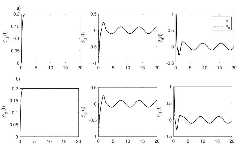
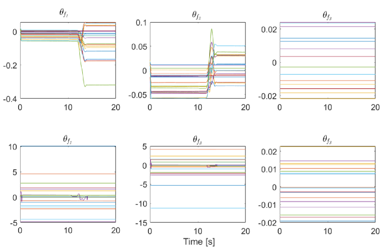
The figures Fig. 14 and Fig. 15 depict the evolution of the fuzzy model’s adaptation parameters. It is clear that parameters converge rapidly to their stationary values. Those peaks are due to system perturbations.

Figure 13: Responses of system with a sinusoidal trajectory

Figure 14: Adaptations of Parameters ${\theta_{g_{\phi}}},{\theta_{g_{\theta}}}$ and ${\theta_{g_{\psi}}}$ in function of time: a)T1FC b)IVFC

Figure 15: Parameters adaptation ${\theta_{f_{\phi}}},{\theta_{f_{\theta}}}$ and ${\theta_{f_{\psi}}}$ in function of time: a)T1FC b)IVFC

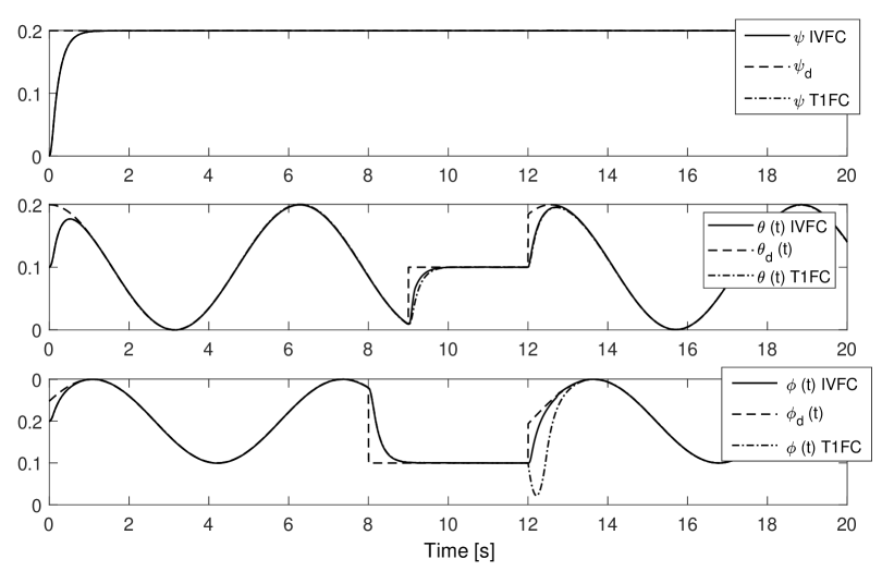
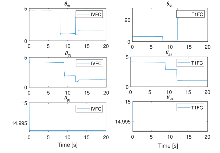
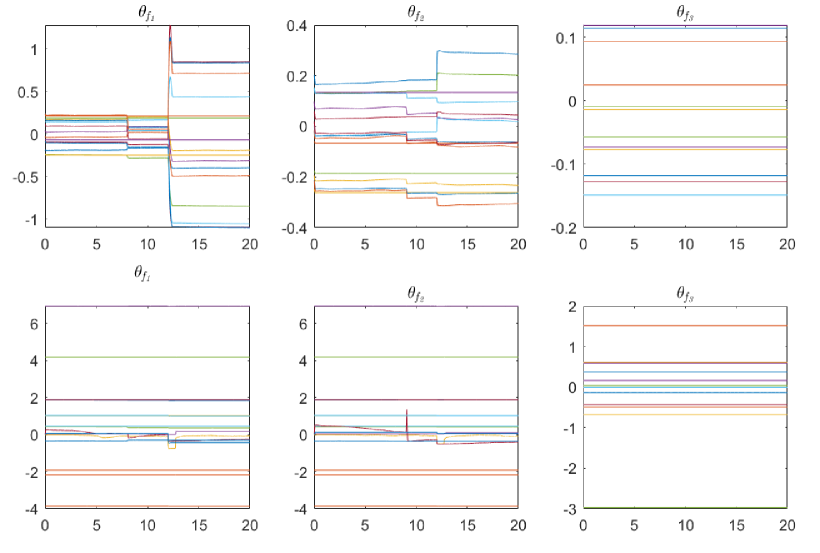
We note that the system met the desired reference. The error of tracking in Fig. 13 and the Table 3 can be explained by the error between the estimated model and the real model. Anyway, the effect of this error is too small, and we note that the error obtained with this approach is minimal.

Table 3: Comparison of MSE between T1 and IVFC

MSE	IVFC	T1FC
$\tilde{\theta}$	22.5090	23.0242
$\tilde{\beta}$	44.9816	81.8549
$\tilde{\psi}$	1.0554	1.0587

5.1.2 Position Control:

we consider the following trajectory:

$${x_{d}}(t)=sin(t)\,,{y_{d}}(t)=sin(t+\pi)\,,{z_{d}}(t)=1\,\,,\,\,{\psi_{d}}(t)=0.2$$

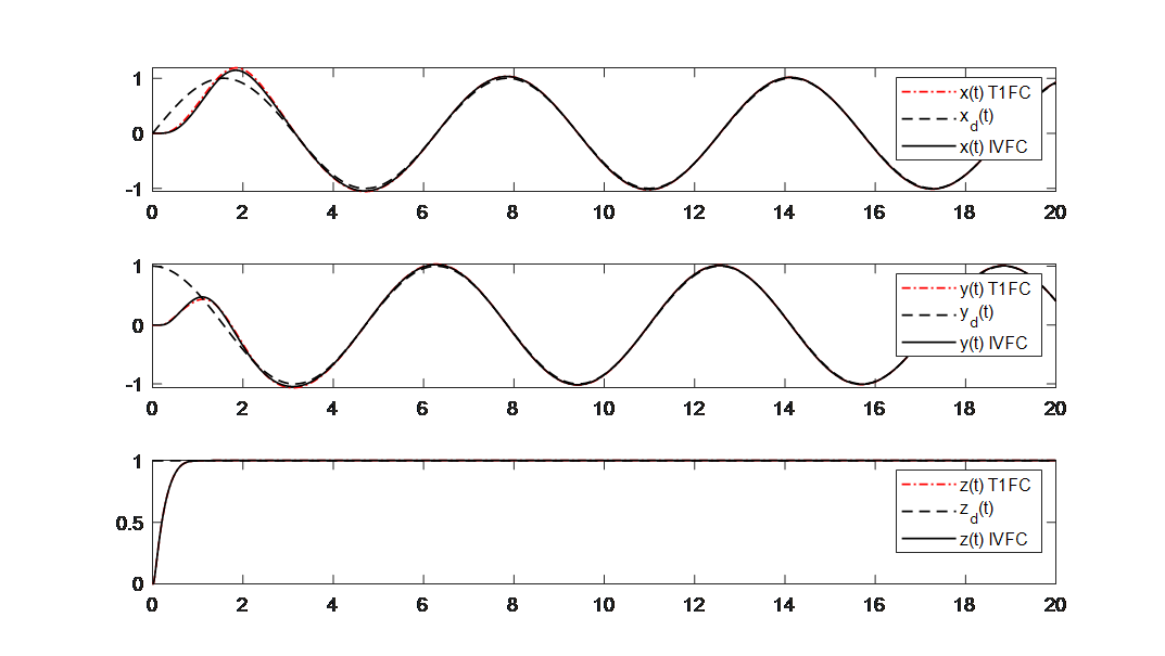
In the absence of any parametric variation in the case of position tracking, the results of simulation are almost identical and sufficiently acceptable Fig. 16. Figure Fig. 17 depicts the angles that correspond to position responses.

Figure 16: response of system with sinusoidal trajectory

Figure 17: correspondent’s Angles to responses of position a) T1FC b) IVFC

5.2 Simulation with Perturbation

5.2.1 Attitude Control:

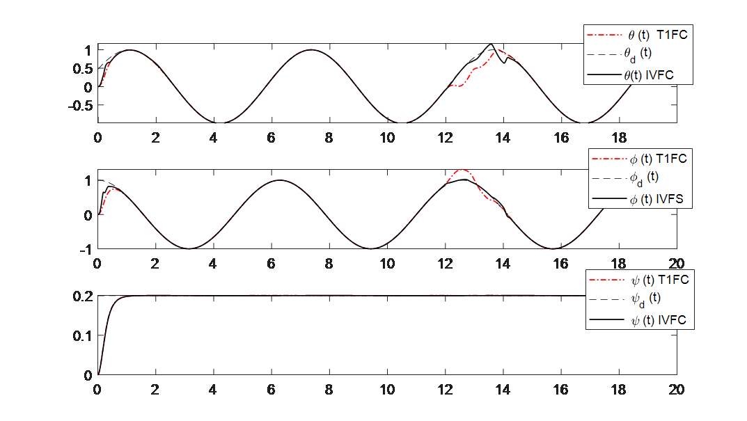
This test is about the application of the control law to a quadrotor with perturbations in the range of time [12s,14s].  This test is carried out by varying $\delta{I}$ and $\delta{J_{r}}$ around the values of the rotor’s inertia ${J_{r}}$ and the drone’s inertia $(I_{xx},I_{yy},I_{zz})$. The variation can be written as ${\hat{J}_{r}}={J_{r}}+\delta{J_{r}}$ and $\hat{I}=I+\delta I$.

Figures (Fig. 18  19 and  20) show the results of tracking for the three tests mentioned above. In the case where we introduce the model disturbance, we note a deviation from the desired consign.

Figure 18: Adaptative Sliding mode control in presence of disturbance $\delta{J_{r}}=10\%{J_{r}}$

Figure 19: Adaptative Sliding mode control in presence of disturbance $\delta{J_{r}}=15\%{J_{r}}$

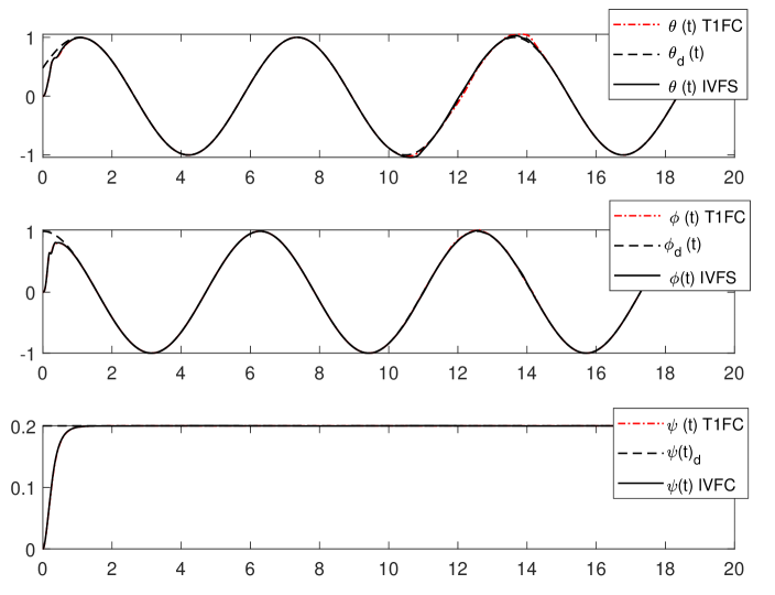
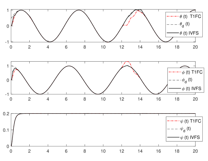
Note that in all simulations, the added perturbations are quickly compensated by the controller IVFC proposed with respect to the conventional type-1 controller. Note also that in Table 4 the rejection of perturbation is more effective, especially when the system has a high level of disturbance.

Table 4: Comparison of MSE between T1 and IVFC

	test 1		test 2		test 3
MSE	IVFC	T1FC	IVFC	T1FC	IVFC	T1FC
$\tilde{\theta}$	7.492	13.216	7.590	9.693	8.060	9.118
$\tilde{\beta}$	17.548	49.829	17.310	32.508	17.295	31.033
$\tilde{\psi}$	1.055	1.056	1.055	1.055	1.055	1.053

Figure 20: Adaptive sliding mode controller in presence of perturbations$\delta{J_{r}}=20\%{J_{r}}$

Figure 21: Evolution of Adaptations parameters of ${f_{i}}(x)$ : a) T1FC b) IVFC

5.2.2 Position Control:

In this simulation, the model is submitted to an external disturbance on the angles ${\varphi_{d}}$ and ${\theta_{d}}$ that attack the position controller. This additive perturbation is chosen to be $\delta\varphi=0.25rad$ in the range [8s 8.5s] and $\delta\theta=0.25rad$ in the range [9s 9.5s], as shown in the Fig. 22. The tracking response of position is shown in Fig. 23 .

Figure 22: Angles correspondent with perturbation $\delta\varphi=\delta\theta=0.25rad$

Figure 23: Response of system using sliding mode adaptative fuzzy model based

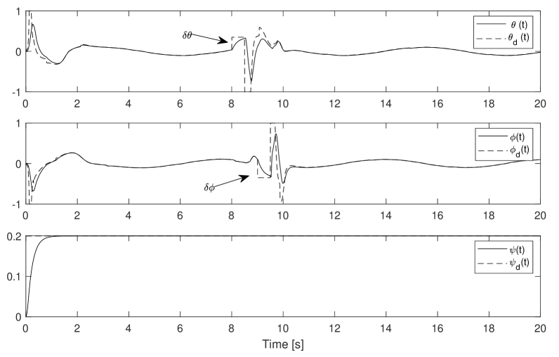
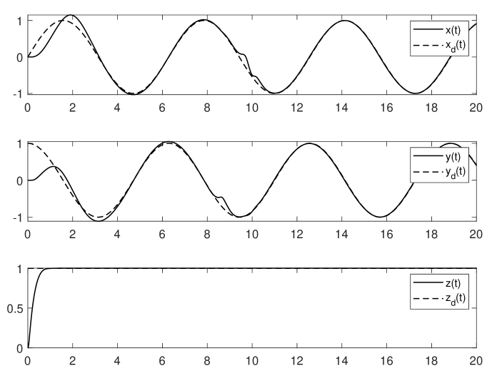
The results of Fig. 23 and the MSE Table 5 show the efficiencies and robustness of the proposed control.

Table 5: Comparison of MSE between T1 and IVFC

MSE	T1FC	IVFC
$\tilde{x}$	46.6442	39.7494
$\tilde{y}$	127.3148	123.8104
$\tilde{z}$	30.7955	30.7955

6 CONCLUSION

In this paper, we presented an algorithm to build an IVFM fuzzy model from input-output data for a nonlinear system. The proposed method for constructing the Takagi-Sugeno (TS) type-2 fuzzy model, based on input-output data of the identified dynamics, is constructed by identifying the structure using fuzzy clustering, then, the envelope detection, and finally the identification of parameters. The proposed method is used to model the unknown parts of the quadrotor dynamics, and the model is then used to design a fuzzy sliding mode adaptive controller in which the unknown dynamics are approximated by an IVFM as an initial model, and the model is then adjusted online using Lyapunov theory-based law. The compared results are presented to demonstrate the effectiveness of the proposed method. Many cases are considered for the sake of showing and testing the performance of tracking and robustness. Finally, the results show that the tracking error has converged despite internal and external disturbances.

References

- H.Mo and Farid [2019] H.Mo and Gh. Farid. Nonlinear and adaptive intelligent control techniques for quadrotor uav. Journal Name, 21(2):989–1008, March 2019.
- Gao et al. [2015] H.and Gao, D. Guo C. Liu, and J. Liu. Fuzzy adaptive pd control for quadrotor helicopter. IEEE Int. Conf. Cyber Technol. Automation Control Intell. Syst. Shenyang, China, 1(5):281–286, May 2015.
- Rabhi et al. [2011] A. Rabhi, M. Chadli, and C. Pegard. Robust fuzzy control for stabilization of a quadrotor. 15th Int. Conf. Adv. Robotics, Tallinn, Estonia, 1(5):471–475, May 2011.
- Niroumand and Seyedsajadi [2013] F. J.and A. Fakharian Niroumand and M. S. Seyedsajadi. Fuzzy integral backstepping control approach in attitude stabilization of a quadrotor uav. 13th Iranian Conf. Fuzzy Syst., Qazvin, Iran, 1(5):1–6, May 2013.
- Pazooki and Mazinan [2017] M. Pazooki and A. H. Mazinan. Hybrid fuzzybased sliding-mode control approach, optimized by genetic algorithm for quadrotor unmanned aerial vehicles. Complex Intell. Syst., 1(5):1–3, May 2017.
- Ul Amin and Kamsin [2017] A. Li M. Umer Khan S. Shamshirband Ul Amin, R. and A. Kamsin. An adaptive trajectory tracking control of four rotor hover vehicle using extended normalized radial basis function network. Mech. Syst. Signal Process., 83:53–74, 2017.
- Dierks and Jagannathan [2010] T. Dierks and S. Jagannathan. Output feedback control of a quadrotor uav using neural networks. IEEE Trans. Neural Netw., 21:50–66, 2010.
- Dierks and Jagannathan [2009] T. Dierks and S. Jagannathan. Neural network control of quadrotor uav formations. Amer. Control Conf. ,St. Louis, MO, USA, 1(5):2990–2996, May 2009.
- Li and Zheng [2016] Y. Wang J. Tan Li, S. and Y. Zheng. Adaptive rbfnns/integral sliding mode control for a quadrotor aircraft. Neurocomputing, 216(5):126–134, May 2016.
- Lee [2021] S.and Kwak S.and You K. Lee, K.and Kim. Quadrotor stabilization and tracking using nonlinear surface sliding mode control and observer. Appl. Sci., 11(5):1–3, May 2021.
- Babuska et al. [1998] R. Babuska, J.A. Roubos, and H.B. Verbruggen. Identification of mimo systems by input–output ts fuzzy models. IEEE Int. Conf. on Fuzzy Systs, Anchorage, AK, USA, 1(5):657–662, 1998.
- Babuska and Verbruggen [1997] R. Babuska and H.B. Verbruggen. Constructing fuzzy models by product space clustering. H. Hellendoorn, D. Driankov (Eds.), Fuzzy Model Identification, Selected Approaches, Springer-Verlag, 1(5):53–90, May 1997.
- Gustafson and Kessel [1979] D.E. Gustafson and W.C. Kessel. Hybrid fuzzybased sliding-mode control approach, optimized by genetic algorithm for quadrotor unmanned aerial vehicles. Fuzzy clustering with a fuzzy covariance matrix, Proc. IEEE CDC, San Diego, CA, 1(5):761–766, May 1979.
- Filho and Serra [2016] O.D. Filho and G.L. Serra. Evolving fuzzy clustering algorithm based on maximum likelihood with participatory learning,. IEEE (EAIS), 1:1–3, May 2016.
- Bouhentala et al. [2017] M. Bouhentala, M. Ghanai, and Kh. Chafaa. Interval-valued membership function estimation for fuzzy modeling. Fuzzy Sets and Systems, 361:101–113, June 2017. doi:doi.org/10.1016/j.fss.2018.06.008.
- Bouabdallah [2007] S. Bouabdallah. design and control of quadrotors with application to autonomous flying. PhD Thesis, Lausanne, EPFL, 2007.
- Sastry and Isidori [1989] S.S Sastry and A. Isidori. Adaptive control of linearizable systems,. IEEE Trans. Automat. Contr., 34:1123–1131, Nov 1989.
- Slotine and Coetsee [1986] J-J E Slotine and Coetsee. Adaptive sliding controller synthesis for nonlinear systems. Int. J. Control, 43(6):1631–1651, 1986.