The role of permanently resident populations in the two-patches SIR model with commuters

Abstract

We consider a two-patches SIR model where communication occurs thru commuters, distinguishing explicitly permanently resident populations from commuters populations. We give an explicit formula of the reproduction number, and show how the proportions of permanently resident populations impact it. We exhibit non-intuitive situations for which allowing commuting from a safe territory to another one where the transmission rate is higher can reduce the overall epidemic threshold and avoid an outbreak.

MSC Classification]92D30, 34D20, 90C31

1 Introduction

Since the pioneer work of Kermack and McKendrick Kermack27 , the SIR model has been very popular in epidemiology, as the basic model for infectious diseases with direct transmission (e.g. Anderson91 ). It retakes great importance nowadays due to the recent coronavirus pandemic. While early models were not spatialized, the importance of accounting for spatial heterogeneity has been often reported in the literature (see, e.g. Angulo79 ; Sattenspiel95 ; Keeling04 ; Keeling07 ; Kelly16 ; Li21 ). However, different mechanisms come into play to explain the spatial spreading of a disease. Although diffusion appears to be a natural process to describe the local propagation of an infectious agent among a population, which leads to models with partial differential equations Murray03 , it appears to be not well suited for describing long distance spreading. In particular, transportation between cities comes into the picture as a major source of rapid spreading among non-homogeneous populations Arino03 ; Arino07 ; Takeuchi07 ; Liu13 ; Mpolya14 ; Chen14 ; Yin20 ; ToctoErazo21 ; Lipshtat21 . Meta-populations or multi-patches models are then more appropriate to describe the spatial characteristics of the propagation Wang03 ; Wang04 ; Arino06 ; Gao07 ; Arino09 , as already well considered in ecology Hanski99 ; McArthur01 . These models require a precise description of the movements between patches, which are most of the time assumed to be linear and thus encoded into a connection matrix Arino06 ; Arino09 . Typically one obtains a system of ordinary differential equations on a graph, which couples the communication dynamics with the epidemiological one.

For diseases spreading among human populations living in different cities, commuters (individuals housing in a city, traveling regularly for short periods in a neighboring city, and coming back to their home city) play a crucial role in the disease propagation among territories Keeling02 ; Keeling04 ; Keeling07 ; Mpolya14 ; Yin20 . Such coupling between patches have been already considered in the literature, distinguishing among populations $N_{i}$ attached to a city $i$ the sub-population $N_{ii}$ present in its permanent housing from other sub-populations $N_{ij}$ temporary present in another city $j\neq i$ (it can be also seen as multi-groups models as in Clancy96 ; Guo06 ; Iggidr12 ). However, such models explicitly assume that the whole population housing in a given city can potentially commute to another one. We believe that this is not always fully realistic and that a sub-population that never (or very rarely) moves to another city should be distinguished from the sub-population that visits at a regular basis another city. Therefore, we consider an extension of such models, which explicitly takes into consideration two kinds of movement: an Eulerian one which describes the flow between patches that mixes populations, and an Lagrangian one which assigns home locations of individuals, as described in the more general framework Citron_etal2021 . The study of this extension, which has not yet been analyzed analytically in the literature, to our knowledge, and how it impacts the disease spreading, is the primary objective of the present work. For this purpose, we establish an analytical expression of the reproduction number (as the epidemic threshold formerly introduced and analyzed in Diekmann90 ; vandenDriessche02 ; Diekmann07 ; Dhirasakdanon07 ) for the two patches case (that is also valid for the particular case when the whole populations travel, for which the exact expression of the reproduction number has not been yet provided in the literature).

We also had in mind to consider heterogeneity among territories when disease transmission differs from one city to another one. Typically, non-pharmaceutical interventions (such as reducing physical distance in the population) could be applied with different strength in each city, providing distinct transmission rates. When one territory being isolated presents a higher reproduction number than the other territory, it can be considered as a core group in the epidemiological terminology Hadeler-Castillo-Chavez1995 ; Brunham1997 , and commuters contribute then to spread the epidemics in both territories. We aim at analyzing more precisely how the proportions of commuters in each city can increase or decrease the overall reproduction number. Intuitively, one may believe that the best way to reduce the spreading is to encourage commuters from the city with the lowest transmission rate not to travel to the other city, and on the opposite to encourage as much as possible commuters from the other city to spend time in the safer city. Indeed, we shall see that this is not always true… The second objective of the present work is thus to study the minimization of the epidemic threshold of the two-patches model with respect to these proportions, depending on the commuting rates. This analysis can potentially serve for decisions making to prevent epidemic outbreak (as in Knipl16 for instance).

The paper is organized as follows. In the next section, we present the complete model in dimension $18$ and give some preliminaries. Section 3 is devoted to the analysis of the asymptotic behavior of the solutions of the model. We give and demonstrate an explicit expression of the reproduction number, introducing four relevant quantities $q_{ij}$ ($i,j=1,2$). In a corollary, we also give an alternative way of computation, which is useful in the following. In Section 4, we study the minimization of the reproduction number with respect to the proportions of commuters in each patch. Finally, Section 5 gives a numerical illustration of the results, considering two territories with intrinsic basic reproduction numbers lower and higher than one. We depict the relative sizes of the permanently resident populations that can avoid the outbreak of the epidemic depending on the commuting rates, and discuss the various cases. We end with a conclusion.

2 The model

We follow the modeling of commuters proposed in Keeling02 between two patches (such as cities or territories), but here we consider in addition that a part of the population in each patch do not commute (the permanently resident sub-population). We consider populations of size $N_{i}$ whose home belongs to a patch $i\in\{1,2\}$, structured in three groups:

1. [i.]

2. permanently resident, being all the time in patch $i$, whose population size is denoted $N_{ir}$,

3. commuters to patch $j$, but located in patch $i$ at time $t$, of population size denoted $N_{ii}$,

4. commuters to patch $j$ and located in patch $j$ at time $t$, of population size denoted $N_{ij}$.

We shall denote $N_{ic}=N_{ii}+N_{ij}$ the size of the total population of commuters with their home in patch $i$. The individuals commutes to patch $j$ at a rate $\lambda_{i}$ with a return rate $\mu_{i}$. For each group $g\in\{ir,ii,ij\}$ we denote by $S_{g}$, $I_{g}$, $R_{g}$ the sizes of susceptible, infected and recovered sub-populations. This modeling implicitly assumes that at any time there is no individual out the territories, that is traveling time is negligible. This assumption is therefore only valid for adjoining territories with short transportation times (by train, road…). It would not be valid between distant territories connected for example by boat or plane with non-negligible crossing times. In this case, it would be necessary to consider additional nodes of in-transit populations, as it has been considered for example in Colizza_etal2013 ; Patil2021 or in Ruan2015 where distance between nodes are explicitly taken into consideration. This would of course complicates the model and its study.

We consider the SIR model assuming that the recovery parameter $\gamma$ is identical everywhere while the transmission rate $\beta_{i}$ depends on the patch $i$ but is identical among each group. Typically lifestyle and hygienic measures may differ between two cities, implying different values of $\beta$. Moreover, if two cities are on both sides of the border between two countries, the strength of non-pharmaceutical interventions are likely to be different, as is was for instance the case between European countries during the SARS-2 outbreak. The model is written as follows (with $i\neq j$ in $\{1,2\}$).

$$\dot{S}_{ir} =-\beta_{i}S_{ir}\frac{I_{ir}+I_{ii}+I_{ji}}{N_{ir}+N_{ii}+N_{ji}},$$

$$\dot{I}_{ir} =\beta_{i}S_{ir}\frac{I_{ir}+I_{ii}+I_{ji}}{N_{ir}+N_{ii}+N_{ji}}-\gamma I_{ir},$$

$$\dot{R}_{ir} =\gamma I_{ir},$$

$$\dot{S}_{ii} =-\beta_{i}S_{ii}\frac{I_{ir}+I_{ii}+I_{ji}}{N_{ir}+N_{ii}+N_{ji}}-\lambda_{i}S_{ii}+\mu_{i}S_{ij},$$

$$\dot{I}_{ii} =\beta_{i}S_{ii}\frac{I_{ir}+I_{ii}+I_{ji}}{N_{ir}+N_{ii}+N_{ji}}-\gamma I_{ii}-\lambda_{i}I_{ii}+\mu_{i}I_{ij},$$

$$\dot{R}_{ii} =\gamma I_{ii}-\lambda_{i}R_{ii}+\mu_{i}R_{ij},$$

$$\dot{S}_{ij} =-\beta_{j}S_{ij}\frac{I_{jr}+I_{jj}+I_{ij}}{N_{jr}+N_{jj}+N_{ij}}+\lambda_{i}S_{ii}-\mu_{i}S_{ij},$$

$$\dot{I}_{ij} =\beta_{j}S_{ij}\frac{I_{jr}+I_{jj}+I_{ij}}{N_{jr}+N_{jj}+N_{ij}}-\gamma I_{ij}+\lambda_{i}I_{ii}-\mu_{i}I_{ij},$$

$$\dot{R}_{ij} =\gamma I_{ij}+\lambda_{i}R_{ii}-\mu_{i}R_{ij}$$

Parameters $\lambda_{i}$, $\mu_{i}$ represent switching rates of populations $i$, leaving home and returning. This modeling implicitly assumes that movements between territories are not synchronized, as often considered in multi-city models (see e.g.  Sattenspiel95 ; Keeling02 ; Arino03 ; Wang03 ; Wang04 ; Keeling04 ; Arino06 ; Takeuchi07 ; Keeling07 ; Liu13 ; Chen14 ). Note that we also consider, in all generality, that commuting is asymmetrical (i.e. $\lambda_{1}$ and $\lambda_{2}$ may be different, as well as $\mu_{1}$, $\mu_{2}$). Typically, each territory may offer different activities that attract commuters from the other territory, and thus different mean sojourn times. One can check that the population sizes $N_{ir}$, and $N_{ic}$ are constant. Moreover $N_{ii}$, $N_{ij}$ fulfill the system of equations

$$\left\{\begin{array}[]{l}\dot{N}_{ii}=-\lambda_{i}N_{ii}+\mu_{i}N_{ij},\\ \dot{N}_{ij}=\lambda_{i}N_{ii}-\mu_{i}N_{ij}\end{array}\right.$$

whose solutions verify

$$\lim_{t\to+\infty}N_{ii}(t)=\bar{N}_{ii}:=\frac{\mu_{i}}{\lambda_{i}+\mu_{i}}N_{ic},\quad\lim_{t\to+\infty}N_{ij}(t)=\bar{N}_{ij}:=\frac{\lambda_{i}}{\lambda_{i}+\mu_{i}}N_{ic}$$ (1)

We shall assume that populations are already balanced at initial time i.e. that one has $N_{ii}=\bar{N}_{ii}$, $N_{ij}=\bar{N}_{ij}$ (constant). For simplicity, we shall drop the notation $\bar{}\,$ in the following, and denote

$$N_{ip}:=N_{ir}+N_{ii}+N_{ji}$$

which represents the (constant) size of the total population present in patch $i$.

3 The epidemic threshold

We denote the vectors

$$I=(I_{1r},I_{11},I_{12},I_{2r},I_{22},I_{21})^{\top},\quad S=(S_{1r},S_{11},S_{12},S_{2r},S_{22},S_{21})^{\top}$$

and consider the state vector

$$X=\left[\begin{array}[]{c}I\\ S\end{array}\right]$$

which belongs to the invariant domain

$${\cal D}:=\{X\in\mathbb{R}_{+}^{12}\mathchar 24635\relax\;\;\mathbb{M}X\leq\mathbb{N}\}$$

where $\mathbb{N}$ is the vector

$$\mathbb{N}=(N_{1r},N_{11},N_{12},N_{2r},N_{22},N_{21})^{\top}$$

and $\mathbb{M}$ the $6\times 12$ matrix which consists in the concatenation of the identity matrix $\mathbb{I}_{6}$ of dimension $6\times 6$

$$\mathbb{M}=[\mathbb{I}_{6},\mathbb{I}_{6}]$$

The disease free equilibrium is defined as

$$X^{\star}=\left[\begin{array}[]{c}0\\ \mathbb{N}\end{array}\right]$$

Let ${\cal R}_{i}$ be the intrinsic reproduction number in the patch $i$ (i.e. when there is no connection between patches), that is

$${\cal R}_{i}:=\frac{\beta_{i}}{\gamma}.$$

We give now an explicit expression of the epidemic threshold when the two patches communicates via commuters.

Proposition 1.

Let

$${\cal R}_{1,2}:=\frac{q_{11}+q_{22}+\sqrt{(q_{22}-q_{11})^{2}+4q_{12}q_{21}}}{2}$$ (2)

where

$$\left\{\begin{array}[]{l}q_{11}={\cal R}_{1}\left(\frac{N_{1r}}{N_{1p}}+\frac{N_{11}}{N_{1p}}\frac{\gamma+\mu_{1}}{\gamma+\lambda_{1}+\mu_{1}}+\frac{N_{21}}{N_{1p}}\frac{\gamma+\lambda_{2}}{\gamma+\lambda_{2}+\mu_{2}}\right)\\ \vskip 6.0pt plus 2.0pt minus 2.0pt\cr q_{22}={\cal R}_{2}\left(\frac{N_{2r}}{N_{2p}}+\frac{N_{22}}{N_{2p}}\frac{\gamma+\mu_{2}}{\gamma+\lambda_{2}+\mu_{2}}+\frac{N_{12}}{N_{2p}}\frac{\gamma+\lambda_{1}}{\gamma+\lambda_{1}+\mu_{1}}\right)\\ \vskip 6.0pt plus 2.0pt minus 2.0pt\cr q_{21}={\cal R}_{1}\left(\frac{N_{11}}{N_{1p}}\frac{\lambda_{1}}{\gamma+\lambda_{1}+\mu_{1}}+\frac{N_{21}}{N_{1p}}\frac{\mu_{2}}{\gamma+\lambda_{2}+\mu_{2}}\right)\\ \vskip 6.0pt plus 2.0pt minus 2.0pt\cr q_{12}={\cal R}_{2}\left(\frac{N_{12}}{N_{2p}}\frac{\mu_{1}}{\gamma+\lambda_{1}+\mu_{1}}+\frac{N_{22}}{N_{2p}}\frac{\lambda_{2}}{\gamma+\lambda_{2}+\mu_{2}}\right)\end{array}\right.$$ (3)

Then, one has the following properties.

1. [i.]

2. If ${\cal R}_{1,2}>1$, then $X^{\star}$ is unstable.

3. If ${\cal R}_{1,2}<1$, then $X^{\star}$ is exponentially stable with respect to the variable $I$.

4. If ${\cal R}_{1}={\cal R}_{2}:={\cal R}$, then ${\cal R}_{1,2}={\cal R}$.

Proof: Write the dynamics of $X$ as $\dot{X}=f(X)$. The Jacobian matrix $J$ of $f$ at $X^{\star}$ is of the form

$$J=\left[\begin{array}[]{cc}A&0\\ \star&B\end{array}\right]\mbox{ with }A=F-V$$

where

$$F=\left[\begin{array}[]{cccccc}\beta_{1}\frac{N_{1r}}{N_{1p}}&\beta_{1}\frac{N_{1r}}{N_{1p}}&0&0&0&\beta_{1}\frac{N_{1r}}{N_{1p}}\\ \vskip 6.0pt plus 2.0pt minus 2.0pt\cr\beta_{1}\frac{N_{11}}{N_{1p}}&\beta_{1}\frac{N_{11}}{N_{1p}}&0&0&0&\beta_{1}\frac{N_{11}}{N_{1p}}\\ \vskip 6.0pt plus 2.0pt minus 2.0pt\cr 0&0&\beta_{2}\frac{N_{12}}{N_{2p}}&\beta_{2}\frac{N_{12}}{N_{2p}}&\beta_{2}\frac{N_{12}}{N_{2p}}&0\\ \vskip 6.0pt plus 2.0pt minus 2.0pt\cr 0&0&\beta_{2}\frac{N_{2r}}{N_{2p}}&\beta_{2}\frac{N_{2r}}{N_{2p}}&\beta_{2}\frac{N_{2r}}{N_{2p}}&0\\ \vskip 6.0pt plus 2.0pt minus 2.0pt\cr 0&0&\beta_{2}\frac{N_{22}}{N_{2p}}&\beta_{2}\frac{N_{22}}{N_{2p}}&\beta_{2}\frac{N_{22}}{N_{2p}}&0\\ \vskip 6.0pt plus 2.0pt minus 2.0pt\cr\beta_{1}\frac{N_{21}}{N_{1p}}&\beta_{1}\frac{N_{21}}{N_{1p}}&0&0&0&\beta_{1}\frac{N_{21}}{N_{1p}}\end{array}\right],$$

$$V=\left[\begin{array}[]{cccccc}\gamma&0&0&0&0&0\\ \vskip 6.0pt plus 2.0pt minus 2.0pt\cr 0&\gamma+\lambda_{1}&-\mu_{1}&0&0&0\\ \vskip 6.0pt plus 2.0pt minus 2.0pt\cr 0&-\lambda_{1}&\gamma+\mu_{1}&0&0&0\\ \vskip 6.0pt plus 2.0pt minus 2.0pt\cr 0&0&0&\gamma&0&0\\ \vskip 6.0pt plus 2.0pt minus 2.0pt\cr 0&0&0&0&\gamma+\lambda_{2}&-\mu_{2}\\ \vskip 6.0pt plus 2.0pt minus 2.0pt\cr 0&0&0&0&-\lambda_{2}&\gamma+\mu_{2}\end{array}\right]$$

and

$$B=\left[\begin{array}[]{cccccc}0&0&0&0&0&0\\ \vskip 6.0pt plus 2.0pt minus 2.0pt\cr 0&-\lambda_{1}&\mu_{1}&0&0&0\\ \vskip 6.0pt plus 2.0pt minus 2.0pt\cr 0&\lambda_{1}&-\mu_{1}&0&0&0\\ \vskip 6.0pt plus 2.0pt minus 2.0pt\cr 0&0&0&0&0&0\\ \vskip 6.0pt plus 2.0pt minus 2.0pt\cr 0&0&0&0&-\lambda_{2}&\mu_{2}\\ \vskip 6.0pt plus 2.0pt minus 2.0pt\cr 0&0&0&0&\lambda_{2}&-\mu_{2}\end{array}\right]$$

Note that $F$ is a non-negative matrix and $V$ is a non-singular M-matrix. We recall (see for instance from vandenDriessche02 ) that one has the property

$$\max Re(Spec(A))\underset{\displaystyle>}{<}0\Longleftrightarrow\rho(FV^{-1})\underset{\displaystyle>}{<}1$$

The computation of the matrix $M:=FV^{-1}$ gives the following expression

$$M=\left[\begin{array}[]{cccccc}{\cal R}_{1}\frac{N_{1r}}{N_{1p}}&{\cal R}_{1}\frac{N_{1r}(\gamma+\mu_{1})}{N_{1p}(\gamma+\lambda_{1}+\mu_{1})}&{\cal R}_{1}\frac{N_{1r}\mu_{1}}{N_{1p}(\gamma+\lambda_{1}+\mu_{1})}&0&{\cal R}_{1}\frac{N_{1r}\lambda_{2}}{N_{1p}(\gamma+\lambda_{2}+\mu_{2})}&{\cal R}_{1}\frac{N_{1r}(\gamma+\lambda_{2})}{N_{1p}(\gamma+\lambda_{2}+\mu_{2})}\\ \vskip 6.0pt plus 2.0pt minus 2.0pt\cr{\cal R}_{1}\frac{N_{11}}{N_{1p}}&{\cal R}_{1}\frac{N_{11}(\gamma+\mu_{1})}{N_{1p}(\gamma+\lambda_{1}+\mu_{1})}&{\cal R}_{1}\frac{N_{11}\mu_{1}}{N_{1p}(\gamma+\lambda_{1}+\mu_{1})}&0&{\cal R}_{1}\frac{N_{11}\lambda_{2}}{N_{1p}(\gamma+\lambda_{2}+\mu_{2})}&{\cal R}_{1}\frac{N_{11}(\gamma+\lambda_{2})}{N_{1p}(\gamma+\lambda_{2}+\mu_{2})}\\ \vskip 6.0pt plus 2.0pt minus 2.0pt\cr 0&{\cal R}_{2}\frac{N_{12}\lambda_{1}}{N_{2p}(\gamma+\lambda_{1}+\mu_{1})}&{\cal R}_{2}\frac{N_{12}(\gamma+\lambda_{1})}{N_{2p}(\gamma+\lambda_{1}+\mu_{1})}&{\cal R}_{2}\frac{N_{12}}{N_{2p}}&{\cal R}_{2}\frac{N_{12}(\gamma+\mu_{2})}{N_{2p}(\gamma+\lambda_{2}+\mu_{2})}&{\cal R}_{2}\frac{N_{12}\mu_{2}}{N_{1p}(\gamma+\lambda_{2}+\mu_{2})}\\ \vskip 6.0pt plus 2.0pt minus 2.0pt\cr 0&{\cal R}_{2}\frac{N_{2r}\lambda_{1}}{N_{2p}(\gamma+\lambda_{1}+\mu_{1})}&{\cal R}_{2}\frac{N_{2r}(\gamma+\lambda_{1})}{N_{2p}(\gamma+\lambda_{1}+\mu_{1})}&{\cal R}_{2}\frac{N_{2r}}{N_{2p}}&{\cal R}_{2}\frac{N_{2r}(\gamma+\mu_{2})}{N_{2p}(\gamma+\lambda_{2}+\mu_{2})}&{\cal R}_{2}\frac{N_{2r}\mu_{2}}{N_{1p}(\gamma+\lambda_{2}+\mu_{2})}\\ \vskip 6.0pt plus 2.0pt minus 2.0pt\cr 0&{\cal R}_{2}\frac{N_{22}\lambda_{1}}{N_{2p}(\gamma+\lambda_{1}+\mu_{1})}&{\cal R}_{2}\frac{N_{22}(\gamma+\lambda_{1})}{N_{2p}(\gamma+\lambda_{1}+\mu_{1})}&{\cal R}_{2}\frac{N_{22}}{N_{2p}}&{\cal R}_{2}\frac{N_{22}(\gamma+\mu_{2})}{N_{2p}(\gamma+\lambda_{2}+\mu_{2})}&{\cal R}_{2}\frac{N_{22}\mu_{2}}{N_{1p}(\gamma+\lambda_{2}+\mu_{2})}\\ \vskip 6.0pt plus 2.0pt minus 2.0pt\cr{\cal R}_{1}\frac{N_{21}}{N_{1p}}&{\cal R}_{1}\frac{N_{21}(\gamma+\mu_{1})}{N_{1p}(\gamma+\lambda_{1}+\mu_{1})}&{\cal R}_{1}\frac{N_{21}\mu_{1}}{N_{1p}(\gamma+\lambda_{1}+\mu_{1})}&0&{\cal R}_{1}\frac{N_{21}\lambda_{2}}{N_{1p}(\gamma+\lambda_{2}+\mu_{2})}&{\cal R}_{1}\frac{N_{21}(\gamma+\lambda_{2})}{N_{1p}(\gamma+\lambda_{2}+\mu_{2})}\par\end{array}\right]$$

Let us consider the diagonal matrix

$$D:=\left[\begin{array}[]{cccccc}{\cal R}_{1}\frac{N_{1r}}{N_{1p}}&\\ &{\cal R}_{1}\frac{N_{11}}{N_{1p}}\\ &&{\cal R}_{2}\frac{N_{12}}{N_{2p}}\\ &&&{\cal R}_{2}\frac{N_{2r}}{N_{2p}}\\ &&&&{\cal R}_{2}\frac{N_{22}}{N_{2p}}\\ &&&&&{\cal R}_{1}\frac{N_{21}}{N_{1p}}\end{array}\right]$$

and the matrix $Q=D^{-1}MD$, whose computation gives the expression

$$Q=\left[\begin{array}[]{cccccc}{\cal R}_{1}\frac{N_{1r}}{N_{1p}}&{\cal R}_{1}\frac{N_{11}(\gamma+\mu_{1})}{N_{1p}(\gamma+\lambda_{1}+\mu_{1})}&{\cal R}_{2}\frac{N_{12}\mu_{1}}{N_{2p}(\gamma+\lambda_{1}+\mu_{1})}&0&{\cal R}_{2}\frac{N_{22}\lambda_{2}}{N_{2p}(\gamma+\lambda_{2}+\mu_{2})}&{\cal R}_{1}\frac{N_{21}(\gamma+\lambda_{2})}{N_{1p}(\gamma+\lambda_{2}+\mu_{2})}\\ \vskip 6.0pt plus 2.0pt minus 2.0pt\cr{\cal R}_{1}\frac{N_{1r}}{N_{1p}}&{\cal R}_{1}\frac{N_{11}(\gamma+\mu_{1})}{N_{1p}(\gamma+\lambda_{1}+\mu_{1})}&{\cal R}_{2}\frac{N_{12}\mu_{1}}{N_{2p}(\gamma+\lambda_{1}+\mu_{1})}&0&{\cal R}_{2}\frac{N_{22}\lambda_{2}}{N_{2p}(\gamma+\lambda_{2}+\mu_{2})}&{\cal R}_{1}\frac{N_{21}(\gamma+\lambda_{2})}{N_{1p}(\gamma+\lambda_{2}+\mu_{2})}\\ \vskip 6.0pt plus 2.0pt minus 2.0pt\cr 0&{\cal R}_{1}\frac{N_{11}\lambda_{1}}{N_{1p}(\gamma+\lambda_{1}+\mu_{1})}&{\cal R}_{2}\frac{N_{12}(\gamma+\lambda_{1})}{N_{2p}(\gamma+\lambda_{1}+\mu_{1})}&{\cal R}_{2}\frac{N_{2r}}{N_{2p}}&{\cal R}_{2}\frac{N_{22}(\gamma+\mu_{2})}{N_{2p}(\gamma+\lambda_{2}+\mu_{2})}&{\cal R}_{1}\frac{N_{21}\mu_{2}}{N_{1p}(\gamma+\lambda_{2}+\mu_{2})}\\ \vskip 6.0pt plus 2.0pt minus 2.0pt\cr 0&{\cal R}_{1}\frac{N_{11}\lambda_{1}}{N_{1p}(\gamma+\lambda_{1}+\mu_{1})}&{\cal R}_{2}\frac{N_{12}(\gamma+\lambda_{1})}{N_{2p}(\gamma+\lambda_{1}+\mu_{1})}&{\cal R}_{2}\frac{N_{2r}}{N_{2p}}&{\cal R}_{2}\frac{N_{22}(\gamma+\mu_{2})}{N_{2p}(\gamma+\lambda_{2}+\mu_{2})}&{\cal R}_{1}\frac{N_{21}\mu_{2}}{N_{1p}(\gamma+\lambda_{2}+\mu_{2})}\\ \vskip 6.0pt plus 2.0pt minus 2.0pt\cr 0&{\cal R}_{1}\frac{N_{11}\lambda_{1}}{N_{1p}(\gamma+\lambda_{1}+\mu_{1})}&{\cal R}_{2}\frac{N_{12}(\gamma+\lambda_{1})}{N_{2p}(\gamma+\lambda_{1}+\mu_{1})}&{\cal R}_{2}\frac{N_{2r}}{N_{2p}}&{\cal R}_{2}\frac{N_{22}(\gamma+\mu_{2})}{N_{2p}(\gamma+\lambda_{2}+\mu_{2})}&{\cal R}_{1}\frac{N_{21}\mu_{2}}{N_{1p}(\gamma+\lambda_{2}+\mu_{2})}\\ \vskip 6.0pt plus 2.0pt minus 2.0pt\cr{\cal R}_{1}\frac{N_{1r}}{N_{1p}}&{\cal R}_{1}\frac{N_{11}(\gamma+\mu_{1})}{N_{1p}(\gamma+\lambda_{1}+\mu_{1})}&{\cal R}_{2}\frac{N_{12}\mu_{1}}{N_{2p}(\gamma+\lambda_{1}+\mu_{1})}&0&{\cal R}_{2}\frac{N_{22}\lambda_{2}}{N_{2p}(\gamma+\lambda_{2}+\mu_{2})}&{\cal R}_{1}\frac{N_{21}(\gamma+\lambda_{2})}{N_{1p}(\gamma+\lambda_{2}+\mu_{2})}\par\end{array}\right]$$

The matrix $Q$ is non-negative and irreducible. By Perron-Frobenius Theorem (see for instance BermanPlemmons ), this matrix admits a unique positive eigenvector (up to a scalar multiplication) that corresponds to the simple (positive) eigenvalue $\ell=\rho(Q)=\rho(M)$.

Note that the rank of $Q$ is two. We posit

$$Y=(1,1,0,0,0,1)^{\top},\quad Z=(0,0,1,1,1,0)^{\top}$$

and define $Q_{Y}$, $Q_{Z}$ the first and third lines, respectively, of the matrix $Q$. Then, for any vector $X\in\mathbb{R}^{6}$, on has one has $QX=(Q_{Y}X)Y+(Q_{Z}X)Z$. We look for an positive eigenvector $X$ of the form $X=\alpha Y+(1-\alpha)Z$ with $\alpha\in(0,1)$. One has then

$$QX =\alpha QY+(1-\alpha)QZ$$

$$=\alpha\big{(}(Q_{Y}Y)Y+(Q_{Z}Y)Z\big{)}+(1-\alpha)\big{(}(Q_{Y}Z)Y+(Q_{Z}Z)Z\big{)}$$

$$=\big{(}\alpha(Q_{Y}Y)+(1-\alpha)(Q_{Y}Z)\big{)}Y+\big{(}\alpha(Q_{Z}Y)+(1-\alpha)(Q_{Z}Z)\big{)}Z$$ (4)

On the other hand, as $X$ is an eigenvector, one has

$$QX=\ell X=\alpha\ell Y+(1-\alpha)\ell Z$$ (5)

The vectors $Y$ and $Z$ being orthogonal, one obtains from (3)-(5) the conditions

$$\left\{\begin{array}[]{l}\alpha Q_{Y}Y+(1-\alpha)Q_{Y}Z=\alpha\ell\\ \alpha Q_{Z}Y+(1-\alpha)Q_{Z}Z=(1-\alpha)\ell\end{array}\right.$$ (6)

Let $r=\frac{1-\alpha}{\alpha}$. Eliminating $\ell$ in the two previous equations, $r$ is the positive solution of the polynomial

$$r^{2}Q_{Y}Z+r(Q_{Y}Y-Q_{Z}Z)-Q_{Z}Y=0$$

and $\ell=Q_{Y}Y+rQ_{Y}Z$. One obtains the expression of the eigenvalue

$$\ell=\frac{Q_{Y}Y+Q_{Z}Z+\sqrt{(Q_{Y}Y-Q_{Z}Z)^{2}+4(Q_{Y}Z)(Q_{Z}Y)}}{2}$$

Finally, from the expression of $Q$, one gets

$$\begin{array}[]{l}q_{11}=Q_{Y}Y={\cal R}_{1}\left(\frac{N_{1r}}{N_{1p}}+\frac{N_{11}}{N_{1p}}\frac{\gamma+\mu_{1}}{\gamma+\lambda_{1}+\mu_{1}}+\frac{N_{21}}{N_{1p}}\frac{\gamma+\lambda_{2}}{\gamma+\lambda_{2}+\mu_{2}}\right)\\ \vskip 6.0pt plus 2.0pt minus 2.0pt\cr q_{22}=Q_{Z}Z={\cal R}_{2}\left(\frac{N_{2r}}{N_{2p}}+\frac{N_{22}}{N_{2p}}\frac{\gamma+\mu_{2}}{\gamma+\lambda_{2}+\mu_{2}}+\frac{N_{12}}{N_{2p}}\frac{\gamma+\lambda_{1}}{\gamma+\lambda_{1}+\mu_{1}}\right)\\ \vskip 6.0pt plus 2.0pt minus 2.0pt\cr q_{21}=Q_{Z}Y={\cal R}_{1}\left(\frac{N_{11}}{N_{1p}}\frac{\lambda_{1}}{\gamma+\lambda_{1}+\mu_{1}}+\frac{N_{21}}{N_{1p}}\frac{\mu_{2}}{\gamma+\lambda_{2}+\mu_{2}}\right)\\ \vskip 6.0pt plus 2.0pt minus 2.0pt\cr q_{12}=Q_{Y}Z={\cal R}_{2}\left(\frac{N_{12}}{N_{2p}}\frac{\mu_{1}}{\gamma+\lambda_{1}+\mu_{1}}+\frac{N_{22}}{N_{2p}}\frac{\lambda_{2}}{\gamma+\lambda_{2}+\mu_{2}}\right)\\ \end{array}$$

and thus $\ell={\cal R}_{1,2}$, which is exactly $\rho(M)$.

i. When ${\cal R}_{1,2}>1$, the matrix $A$ has at least one eigenvalue with positive real part and the matrix $J$ as well. The equilibrium $X^{\star}$ is thus unstable on ${\cal D}$.

ii. When ${\cal R}_{1,2}<1$, the matrix $A$ is Hurwitz, but $X^{\star}$ is not an hyperbolic equilibrium. However, on can write the dynamics of the vector $I$ as an non-autonomous system

$$\dot{I}=g(t,I):=\left(\begin{array}[]{c}\beta_{1}S_{1r}(t)\frac{I_{1r}+I_{11}+I_{21}}{N_{1p}}-\gamma I_{1r}\\ \vskip 6.0pt plus 2.0pt minus 2.0pt\cr\beta_{1}S_{11}(t)\frac{I_{1r}+I_{11}+I_{21}}{N_{1p}}-(\gamma+\lambda_{1})I_{11}+\mu_{1}I_{12}\\ \vskip 6.0pt plus 2.0pt minus 2.0pt\cr\beta_{2}S_{12}(t)\frac{I_{2r}+I_{22}+I_{12}}{N_{2p}}+\lambda_{1}I_{11}-(\gamma+\mu_{1})I_{12}\\ \vskip 6.0pt plus 2.0pt minus 2.0pt\cr\beta_{2}S_{2r}(t)\frac{I_{2r}+I_{22}+I_{12}}{N_{2p}}-\gamma I_{2r}\\ \vskip 6.0pt plus 2.0pt minus 2.0pt\cr\beta_{2}S_{22}(t)\frac{I_{2r}+I_{22}+I_{12}}{N_{2p}}-(\gamma+\lambda_{2})I_{22}+\mu_{2}I_{21}\\ \vskip 6.0pt plus 2.0pt minus 2.0pt\cr\beta_{1}S_{21}(t)\frac{I_{1r}+I_{11}+I_{21}}{N_{1p}}+\lambda_{2}I_{22}-(\gamma+\mu_{2})I_{21}\end{array}\right)$$

Note that this dynamics is cooperative and as for any $t\geq 0$ one has $S_{ij}(t)\leq N_{ij}$ for $ij\in\{1r,11,12,2r,22,21\}$, one gets

$$g(t,I)\leq\bar{g}(I):=AI,\;I\geq 0$$

Therefore, any solution $I(\cdot)$ of $\dot{I}=g(t,I)$ with $I(0)=I_{0}\geq 0$ verifies $0\leq I(t)\leq\bar{I}(t)$ for any $t\geq 0$, where $\bar{I}(\cdot)$ is solution of the linear dynamics $\dot{\bar{I}}=\bar{g}(\bar{I})$ with $\bar{I}(0)=I_{0}$. As $A$ is Hurwitz, we conclude that $X^{\star}$ is exponentially stable with respect to $I$, which proves point ii.

iii. For the particular case ${\cal R}_{1}={\cal R}_{2}:={\cal R}$, the transpose of the matrix $M$ writes

$$M^{\top}={\cal R}\left[\begin{array}[]{cccccc}\frac{N_{1r}}{N_{1p}}&\frac{N_{11}}{N_{1p}}&0&0&0&\frac{N_{21}}{N_{1p}}\\ \vskip 6.0pt plus 2.0pt minus 2.0pt\cr\frac{N_{1r}(\gamma+\mu_{1})}{N_{1p}(\gamma+\lambda_{1}+\mu_{1})}&\frac{N_{11}(\gamma+\mu_{1})}{N_{1p}(\gamma+\lambda_{1}+\mu_{1})}&\frac{N_{12}\lambda_{1}}{N_{2p}(\gamma+\lambda_{1}+\mu_{1})}&\frac{N_{2r}\lambda_{1}}{N_{2p}(\gamma+\lambda_{1}+\mu_{1})}&\frac{N_{22}\lambda_{1}}{N_{2p}(\gamma+\lambda_{1}+\mu_{1})}&\frac{N_{21}(\gamma+\mu_{1})}{N_{1p}(\gamma+\lambda_{1}+\mu_{1})}\\ \vskip 6.0pt plus 2.0pt minus 2.0pt\cr\frac{N_{1r}\mu_{1}}{N_{1p}(\gamma+\lambda_{1}+\mu_{1})}&\frac{N_{11}\mu_{1}}{N_{1p}(\gamma+\lambda_{1}+\mu_{1})}&\frac{N_{12}(\gamma+\lambda_{1})}{N_{2p}(\gamma+\lambda_{1}+\mu_{1})}&\frac{N_{2r}(\gamma+\lambda_{1})}{N_{2p}(\gamma+\lambda_{1}+\mu_{1})}&\frac{N_{22}(\gamma+\lambda_{1})}{N_{2p}(\gamma+\lambda_{1}+\mu_{1})}&\frac{N_{21}\mu_{1}}{N_{1p}(\gamma+\lambda_{1}+\mu_{1})}\\ \vskip 6.0pt plus 2.0pt minus 2.0pt\cr 0&0&\frac{N_{12}}{N_{2p}}&\frac{N_{2r}}{N_{2p}}&\frac{N_{22}}{N_{2p}}&0\\ \vskip 6.0pt plus 2.0pt minus 2.0pt\cr\frac{N_{1r}\lambda_{2}}{N_{1p}(\gamma+\lambda_{2}+\mu_{2})}&\frac{N_{11}\lambda_{2}}{N_{1p}(\gamma+\lambda_{2}+\mu_{2})}&\frac{N_{12}(\gamma+\mu_{2})}{N_{2p}(\gamma+\lambda_{2}+\mu_{2})}&\frac{N_{2r}(\gamma+\mu_{2})}{N_{2p}(\gamma+\lambda_{2}+\mu_{2})}&\frac{N_{22}(\gamma+\mu_{2})}{N_{2p}(\gamma+\lambda_{2}+\mu_{2})}&\frac{N_{21}\lambda_{2}}{N_{1p}(\gamma+\lambda_{2}+\mu_{2})}\\ \vskip 6.0pt plus 2.0pt minus 2.0pt\cr\frac{N_{1r}(\gamma+\lambda_{2})}{N_{1p}(\gamma+\lambda_{2}+\mu_{2})}&\frac{N_{11}(\gamma+\lambda_{2})}{N_{1p}(\gamma+\lambda_{2}+\mu_{2})}&\frac{N_{12}\mu_{2}}{N_{1p}(\gamma+\lambda_{2}+\mu_{2})}&\frac{N_{2r}\mu_{2}}{N_{1p}(\gamma+\lambda_{2}+\mu_{2})}&\frac{N_{22}\mu_{2}}{N_{1p}(\gamma+\lambda_{2}+\mu_{2})}&\frac{N_{21}(\gamma+\lambda_{2})}{N_{1p}(\gamma+\lambda_{2}+\mu_{2})}\par\end{array}\right]$$

One can check that one has $M^{\top}U={\cal R}U$ where $U=(1,1,1,1,1,1)^{\top}$. As $U$ is a positive vector, we deduce from the Perron-Frobenius Theorem that one has $\rho(M)=\rho(M^{T})={\cal R}$, which ends the proof.

Remark 1.

More generally, the next-generation matrix $M=FV^{-1}$ can be shown to have a rank equal to the number $n$ of patches, and that its Perron vector can be expressed as a convex combination of a family of orthogonal vectors in the image of $M$. This implies that the positive eigenvalue of $M$ (i.e. the reproduction number) is also the positive eigenvalue of the $n$-dimensional positive matrix given by the decomposition of the image of this vectors by the matrix $M$.
Alternatively, one may consider the epidemic spread in a virgin population as a Markov process, to determine the expected numbers of secondary cases in each patch, and obtain this $n\times n$ matrix, as described in Diekman_etal2013 . This method consists in a first-step analysis by determining the mean residence times of an infected individual of each group in each of the patches. Then, for a given patch the expected numbers of new infected present in each path are given by the products of the mean residence times by the transmission rate, averaged by the constant distribution given in (1).
This explains why the formula (2) takes the expression of a root of the characteristic polynomial of a $2$ by $2$ matrix.

Remark 2.

The explicit expression (2) of the epidemic threshold given in Proposition 1 is also relevant in absence of permanently resident populations, which has not been yet provided explicitly in the literature (up to our knowledge).

Corollary 2.

One has

$$\min\left({\cal R}_{1},{\cal R}_{2}\right)\leq{\cal R}_{1,2}\leq\max\left({\cal R}_{1},{\cal R}_{2}\right).$$

Proof: Denote by $M({\cal R}_{1},{\cal R}_{2})$ the matrix $FV^{-1}$ for the parameters ${\cal R}_{1}$, ${\cal R}_{2}$, and let ${\cal R}_{-}:=\min\left({\cal R}_{1},{\cal R}_{2}\right)$, ${\cal R}_{+}:=\max\left({\cal R}_{1},{\cal R}_{2}\right)$. From the expression of the non-negative matrices $M$, one gets

$$M({\cal R}_{-},{\cal R}_{-})\leq M({\cal R}_{1},{\cal R}_{2})\leq M({\cal R}_{+},{\cal R}_{+})$$

which implies (see for instance BermanPlemmons ) the inequalities

$$\rho(M({\cal R}_{-},{\cal R}_{-}))\leq\rho(M({\cal R}_{1},{\cal R}_{2}))\leq\rho(M({\cal R}_{+},{\cal R}_{+}))$$

and thus

$${\cal R}_{-}\leq{\cal R}_{1,2}\leq{\cal R}_{+}.$$

Alternatively, the number ${\cal R}_{1,2}$ can be determined as follows.

Corollary 3.

Assume ${\cal R}_{2}>{\cal R}_{1}$. Then, one has

$${\cal R}_{1,2}=\alpha{\cal R}_{1}+(1-\alpha){\cal R}_{2}$$ (7)

where $\alpha\in[0,1)$ is the smallest root of the polynomial

$$P(\alpha)=\alpha^{2}({\cal R}_{2}-{\cal R}_{1})-\alpha({\cal R}_{2}-{\cal R}_{1}+q_{12}+q_{21})+q_{12}$$

Proof: One can check, from expressions (3), that one has $q_{11}+q_{21}={\cal R}_{1}$ and $q_{22}+q_{12}={\cal R}_{2}$. Then, from (6), one get

$${\cal R}_{1,2}=l=\alpha{\cal R}_{1}+(1-\alpha){\cal R}_{2}$$ (8)

where $\alpha$ is a root of the polynomial $P$ obtained from (6) by eliminating $l$, that is

$$P(\alpha)=\alpha^{2}({\cal R}_{2}-{\cal R}_{1})-\alpha({\cal R}_{2}-{\cal R}_{1}+q_{12}+q_{21})+q_{12}$$

From Corollary 2, we know that $\alpha$ belongs to $[0,1]$. Note that one has $P(0)=q_{12}\geq 0$ and $P(1)=-q_{21}\leq 0$. Therefore, when ${\cal R}_{2}-{\cal R}_{1}>0$, $P$ admits exactly one root in $[0,1)$ and another one in $[1,\to)$. However, if $\alpha=1$ one should have $q_{21}=0$ and thus $\lambda_{1}=0$, $\mu_{2}=0$, which implies $N_{11}=N_{1c}$, $N_{12}=0$, $N_{22}=0$, $N_{21}=N_{2c}$. Then, one obtains $q_{11}={\cal R}_{1}$, $q_{22}={\cal R}_{2}$ and from the expression (2) on gets ${\cal R}_{1,2}=\max({\cal R}_{1},{\cal R}_{2})={\cal R}_{2}$ which contradicts $\alpha=1$. We conclude that $\alpha$ belongs to $[0,1)$ and is thus the smallest root of $P$.

Remark 3.

When there is no communication between patches (that is $N_{1r}=N_{1p}=N_{1}$, $N_{2r}=N_{2p}=N_{2}$), one has $q_{21}=0$ and $q_{12}=0$. If ${\cal R}_{2}>{\cal R}_{1}$, resp. ${\cal R}_{1}>{\cal R}_{2}$, one has $\alpha=0$, resp. $\alpha=1$, which gives

$${\cal R}_{1,2}=\max({\cal R}_{1},{\cal R}_{2}).$$

We look now for a characterization of the minimum value of the threshold ${\cal R}_{1,2}$.

4 Minimization of the epidemic threshold

In this section, we assume that the mixing is fast compared to the recovery rate (as its is often considered in the literature), which amounts to have numbers $\lambda_{i}$, $\mu_{i}$ large compared to $\gamma$. Our objective is to study how the proportions of commuters in the populations impact the value of ${\cal R}_{1,2}$.

Given ${\cal R}_{1}$, ${\cal R}_{2}$, we consider the approximation $\tilde{\cal R}_{1,2}$ of the threshold ${\cal R}_{1,2}$ which consists in keeping $\gamma=0$ in the expressions (3). For convenience, we posit the numbers

$$\eta_{i}:=\frac{\lambda_{i}}{\lambda_{i}+\mu_{i}}\in(0,1)\qquad(i=1,2)$$

One has a first result about the variations of $\tilde{\cal R}_{1,2}$ with respect to $N_{1c}$, $N_{2c}$.

Proposition 4.

Fix parameters $N_{i}$, $\beta_{i}$, $\gamma$, $\lambda_{i}$, $\mu_{i}$ ($i=1,2$) such that ${\cal R}_{2}>{\cal R}_{1}$.

1. [i.]

2. For any $N_{1c}\in(0,N_{1})$, the map $N_{2c}\mapsto\tilde{\cal R}_{1,2}(N_{1c},N_{2c})$ is decreasing.

3. The map $N_{1c}\mapsto\tilde{\cal R}_{1,2}(N_{1c},N_{2c})$ is increasing at $(N_{1c},N_{2c})$ when

   $$\eta_{2}(1-\eta_{2})N_{2c}>(1-\eta_{1})(N_{2}-\eta_{2}N_{2c})$$ (9)

4. The map $N_{1c}\mapsto\tilde{\cal R}_{1,2}(N_{1c},N_{2c})$ is increasing, resp. decreasing, at $(N_{1c},N_{2c})$ if the numbers $A$ and $B$ are negative, resp. positive, where

   $$A:={\cal R}_{2}\frac{\frac{N_{2}}{2}-\eta_{1}(\frac{1}{2}-\eta_{1})N_{1c}-(\frac{3}{2}-\eta_{2})\eta_{2}N_{2c}}{N_{2}-\eta_{2}N_{2c}+\eta_{1}N_{1c}}$$

   $$\hskip 85.35826pt-{\cal R}_{1}\frac{\frac{N_{1}}{2}-(\frac{3}{2}-\eta_{1})\eta_{1}N_{1c}-\eta_{2}(\frac{1}{2}-\eta_{2})N_{2c}}{N_{1}-\eta_{1}N_{1c}+\eta_{2}N_{2c}},$$

   $$B:={\cal R}_{2}\frac{(1-\eta_{1})(N_{2}-\eta_{2}N_{2c})-\eta_{2}(1-\eta_{2})N_{2c}}{(N_{2}-\eta_{2}N_{2c}+\eta_{1}N_{1c})^{2}}$$

   $$\hskip 85.35826pt-{\cal R}_{1}\frac{(1-\eta_{1})(N_{1}+\eta_{2}N_{2c})+\eta_{2}(1-\eta_{2})N_{2c}}{(N_{1}-\eta_{1}N_{1c}+\eta_{2}N_{2c})^{2}}$$

Proof: Following Corollary 3, one has

$$\tilde{\cal R}_{1,2}=\tilde{\alpha}{\cal R}_{1}+(1-\tilde{\alpha}){\cal R}_{2}$$ (10)

where $\tilde{\alpha}$ is the smallest root of the polynomial

$$\tilde{P}(\alpha)=\alpha^{2}({\cal R}_{2}-{\cal R}_{1})-\alpha({\cal R}_{2}-{\cal R}_{1}+\tilde{q}_{12}+\tilde{q}_{21})+\tilde{q}_{12}$$

where $\tilde{q}_{12}$, $\tilde{q}_{21}$ are the approximations of $q_{12}$, $q_{21}$ defined in (3). Let us note that one can write $N_{ii}=(1-\eta_{i})N_{ic}$, $N_{ij}=\eta_{i}N_{ic}$ (for $j\neq i$) and also $N_{ip}=N_{i}-\eta_{i}N_{ic}+\eta_{j}N_{jc}$, which leads to the following expressions of $\tilde{q}_{12}$, $\tilde{q}_{21}$

$$\tilde{q}_{21}={\cal R}_{1}\frac{(1-\eta_{1})\eta_{1}N_{1c}+\eta_{2}(1-\eta_{2})N_{2c}}{N_{1}-\eta_{1}N_{1c}+\eta_{2}N_{2c}},\quad\tilde{q}_{12}={\cal R}_{2}\frac{\eta_{1}(1-\eta_{1})N_{1c}+(1-\eta_{2})\eta_{2}N_{2c}}{N_{2}-\eta_{2}N_{2c}+\eta_{1}N_{1c}}$$ (11)

For simplicity, we shall drop the notation $\tilde{}\;$ in the rest of the proof. Note than $\alpha$ being the smallest root of $P$, it verifies

$$\alpha<\frac{{\cal R}_{2}-{\cal R}_{1}+q_{12}+q_{21}}{2({\cal R}_{2}-{\cal R}_{1})}$$ (12)

Let us differentiate the equality $P(\alpha)=0$ with respect to $q_{12}$ and $q_{21}$:

$$2\alpha\frac{\partial\alpha}{\partial q_{12}}({\cal R}_{2}-{\cal R}_{1})-\frac{\partial\alpha}{\partial q_{12}}({\cal R}_{2}-{\cal R}_{1}+q_{12}+q_{21})-\alpha+1=0$$

$$2\alpha\frac{\partial\alpha}{\partial q_{21}}({\cal R}_{2}-{\cal R}_{1})-\frac{\partial\alpha}{\partial q_{21}}({\cal R}_{2}-{\cal R}_{1}+q_{12}+q_{21})-\alpha=0$$

which gives

$$\frac{\partial\alpha}{\partial q_{12}}=\frac{1-\alpha}{{\cal R}_{2}-{\cal R}_{1}+q_{12}+q_{21}-2\alpha({\cal R}_{2}-{\cal R}_{1})}$$

$$\frac{\partial\alpha}{\partial q_{21}}=\frac{-\alpha}{{\cal R}_{2}-{\cal R}_{1}+q_{12}+q_{21}-2\alpha({\cal R}_{2}-{\cal R}_{1})}$$

Then, one can write

$$\frac{\partial\alpha}{\partial N_{ic}}=\frac{\partial\alpha}{\partial q_{12}}\frac{\partial q_{12}}{\partial N_{ic}}+\frac{\partial\alpha}{\partial q_{21}}\frac{\partial q_{21}}{\partial N_{ic}}\\ =\frac{(1-\alpha)\frac{\partial q_{12}}{\partial N_{ic}}-\alpha\frac{\partial q_{21}}{\partial N_{ic}}}{{\cal R}_{2}-{\cal R}_{1}+q_{12}+q_{21}-2\alpha({\cal R}_{2}-{\cal R}_{1})}\qquad(i=1,2)$$

and from inequality (12), we obtain that the signs of the derivatives $\frac{\partial\alpha}{\partial N_{ic}}$ are given by the sign of the numbers

$$\sigma_{i}:=(1-\alpha)\frac{\partial q_{12}}{\partial N_{ic}}-\alpha\frac{\partial q_{21}}{\partial N_{ic}}\qquad(i=1,2)$$ (13)

We begin by the dependency with respect to $N_{2c}$. One has first

$$\frac{\partial q_{12}}{\partial N_{2c}}={\cal R}_{2}\eta_{2}\frac{(1-\eta_{2})(N_{2}+\eta_{1}N_{1c})+\eta_{1}(1-\eta_{1})N_{1c}}{(N_{2}+\eta_{1}N_{1c}-\eta_{2}N_{2c})^{2}}>0$$

Note that one has

$$q_{21}=\frac{{\cal R}_{1}(N_{2}+\eta_{1}N_{1c}-\eta_{2}N_{2c})}{{\cal R}_{2}(N_{1}-\eta_{1}N_{1c}+\eta_{2}N_{2c})}q_{12}$$ (14)

and thus

$$\frac{\partial q_{21}}{\partial N_{2c}}=\frac{{\cal R}_{1}(N_{2}+\eta_{1}N_{1c}-\eta_{2}N_{2c})}{{\cal R}_{2}(N_{1}-\eta_{1}N_{1c}+\eta_{2}N_{2c})}\frac{\partial q_{12}}{\partial N_{2c}}-\frac{{\cal R}_{1}\eta_{2}(N_{1}+N_{2})}{{\cal R}_{2}(N_{1}-\eta_{1}N_{1c}+\eta_{2}N_{2c})^{2}}q_{12}$$

Then, one gets the inequality

$$\sigma_{2}>\left(1-\alpha-\alpha\frac{{\cal R}_{1}(N_{2}+\eta_{1}N_{1c}-\eta_{2}N_{2c})}{{\cal R}_{2}(N_{1}-\eta_{1}N_{1c}+\eta_{2}N_{2c})}\right)\frac{\partial q_{12}}{\partial N_{2c}}$$

On another hand, one gets from $P(\alpha)=0$ the inequality

$$(1-\alpha)q_{12}-\alpha q_{21}=\alpha(1-\alpha)({\cal R}_{2}-{\cal R}_{1})>0$$

and with (14)

$$(1-\alpha)q_{12}-\alpha q_{21}=\left(1-\alpha-\alpha\frac{{\cal R}_{1}(N_{2}+\eta_{1}N_{1c}-\eta_{2}N_{2c})}{{\cal R}_{2}(N_{1}-\eta_{1}N_{1c}+\eta_{2}N_{2c})}\right)q_{12}>0$$

We then conclude that $\sigma_{2}$ is positive, and from (10) we deduce that the map $N_{2c}\mapsto{\cal R}_{1,2}$ is decreasing. This proves the point i.

We study now the dependency with respect to $N_{1c}$. A calculation of the partial derivative gives

$$\frac{\partial q_{12}}{\partial N_{1c}}={\cal R}_{2}\eta_{1}\frac{(1-\eta_{1})(N_{2}-\eta_{2}N_{2c})-\eta_{2}(1-\eta_{2})N_{2c}}{(N_{2}-\eta_{2}N_{2c}+\eta_{1}N_{1c})^{2}}$$ (15)

and

$$\frac{\partial q_{21}}{\partial N_{1c}}={\cal R}_{1}\eta_{1}\frac{(1-\eta_{1})(N_{1}+\eta_{2}N_{2c})+\eta_{2}(1-\eta_{2})N_{2c}}{(N_{1}-\eta_{1}N_{1c}+\eta_{2}N_{2c})^{2}}>0$$ (16)

When $\frac{\partial q_{12}}{\partial N_{1c}}<0$, we can conclude that $\sigma_{1}$ is negative and ${\cal R}_{1,2}$ is thus increasing with respect to $N_{1c}$. This condition is equivalent to (9). This proves the point ii. When this last condition is not satisfied, having $\frac{\partial q_{12}}{\partial N_{1c}}<\frac{\partial q_{21}}{\partial N_{1c}}$ with $\alpha>\frac{1}{2}$ is another sufficient condition to obtain $\sigma_{1}<0$ from expression (13). However, having $\alpha>\frac{1}{2}$ amounts to have $P(\frac{1}{2})>0$, that is

$$\frac{{\cal R}_{2}-{\cal R}_{1}}{4}-\frac{{\cal R}_{2}-{\cal R}_{1}+q_{12}+q_{21}}{2}+q_{12}>0$$

or equivalently

$$\frac{{\cal R}_{2}}{2}-q_{12}<\frac{{\cal R}_{1}}{2}-q_{21}$$

One can check that this last condition is equivalent to $A<0$ and that the condition $\frac{\partial q_{12}}{\partial N_{1c}}<\frac{\partial q_{21}}{\partial N_{1c}}$ is equivalent to $B<0$. In the same manner, having $A>0$ and $B>0$ implies $\alpha<\frac{1}{2}$ and $\frac{\partial q_{12}}{\partial N_{1c}}>\frac{\partial q_{21}}{\partial N_{1c}}$, which is a sufficient condition to have $\sigma_{1}>0$, and thus ${\cal R}_{1,2}$ increasing with respect to $N_{1c}$. This proves the point iii.

This result suggests that the map $N_{1c}\mapsto\tilde{\cal R}_{1,2}(N_{1c},N_{2c})$ is not necessarily monotonic, differently to the map $N_{2c}\mapsto\tilde{\cal R}_{1,2}(N_{1c},N_{2c})$. We show now that the possibilities of its variations are limited.

Proposition 5.

Under hypotheses of Proposition 4, for each $N_{2c}\in(0,N_{2})$ the map $N_{1c}\mapsto\tilde{\cal R}_{1,2}(N_{1c},N_{2c})$ possesses one of the three properties

1. [a.]

2. it is decreasing on $(0,N_{1})$,

3. it is increasing on $(0,N_{1})$,

4. there exists $N_{1c}^{\star}\in(0,N_{1})$ such that it is decreasing on $(0,N_{1c}^{\star})$ and increasing on $(N_{1c}^{\star},N_{1})$.

Proof: Fix $N_{2c}\in(0,N_{2})$. If the map $N_{1c}\mapsto\tilde{\cal R}_{1,2}(N_{1c},N_{2c})$ is not monotonic, there exists $\hat{N}_{1c}\in(0,N_{1})$ such that $\frac{\partial\tilde{\cal R}_{1,2}}{\partial N_{1c}}(\hat{N}_{1c},N_{2c})=0$. For simplicity, we shall drop the notation $\tilde{}\;$ in the rest of the proof. Following the proof of Proposition 4, one has ${\cal R}_{1,2}=\alpha{\cal R}_{1}+(1-\alpha){\cal R}_{2}$ with

$$\frac{\partial\alpha}{\partial N_{1c}}=\frac{(1-\alpha)\frac{\partial q_{12}}{\partial N_{1c}}-\alpha\frac{\partial q_{21}}{\partial N_{1c}}}{{\cal R}_{2}-{\cal R}_{1}+q_{12}+q_{21}-2\alpha({\cal R}_{2}-{\cal R}_{1})}:=\frac{\sigma_{1}}{\nu}$$

where $\nu>0$. Therefore, one has $\frac{\partial\alpha}{\partial N_{1c}}=0$ and $\sigma_{1}=0$ at $N_{1c}=\hat{N}_{1c}$, and thus

$$\left.\frac{\partial^{2}\alpha}{\partial N_{1c}^{2}}\right|_{N_{1c}=\hat{N}_{1c}}=\left.\frac{\frac{\partial\sigma_{1}}{\partial N_{1c}}}{\nu}\right|_{N_{1c}=\hat{N}_{1c}}=\left.\frac{(1-\alpha)\frac{\partial^{2}q_{12}}{\partial N_{1c}^{2}}-\alpha\frac{\partial^{2}q_{21}}{\partial N_{1c}^{2}}}{\nu}\right|_{N_{1c}=\hat{N}_{1c}}$$

From expressions (15) and (16), a calculation of the partial derivatives gives

$$\frac{\partial^{2}q_{12}}{\partial N_{1c}^{2}}=\frac{-2\eta_{1}\frac{\partial q_{12}}{\partial N_{1c}}}{N_{1}-\eta_{1}N_{1c}+\eta_{2}N_{2c}},\quad\frac{\partial^{2}q_{21}}{\partial N_{1c}^{2}}=\frac{2\eta_{1}\frac{\partial q_{21}}{\partial N_{1c}}}{N_{2}-\eta_{2}N_{2c}+\eta_{1}N_{1c}}$$

where $\frac{\partial q_{21}}{\partial N_{1c}}>0$ and from $\sigma_{1}=0$ one gets $\frac{\partial q_{12}}{\partial N_{1c}}>0$ for $N_{1c}=\hat{N}_{1c}$. Finally, one obtains

$$\frac{\partial^{2}{\cal R}_{1,2}}{\partial N_{1c}^{2}}(\hat{N}_{1c},N_{2c})=-({\cal R}_{2}-{\cal R}_{1})\frac{\partial^{2}\alpha}{\partial N_{1c}^{2}}(\hat{N}_{1c},N_{2c})<0$$

Consequently, any extremum of the map $N_{1c}\mapsto{\cal R}_{1,2}(N_{1c},N_{2c})$ is a local minimizer, which implies that this map has at most one local minimizer.

Finally, we give conditions for which the minimization of the threshold ${\cal R}_{1,2}$ presents a trichotomy.

Proposition 6.

Let parameters $\beta_{i}$, $\gamma$ be such that ${\cal R}_{2}>{\cal R}_{1}$ and assume that $N_{1}$, $N_{2}$ satisfy $N_{1}{\cal R}_{2}>N_{2}{\cal R}_{1}$. Then, provided that $\gamma$ is small enough compared to $\lambda_{i}$ and $\mu_{i}$, the function $(N_{1c},N_{2c})\mapsto{\cal R}_{1,2}(N_{1c},N_{2c})$ admits an unique minimum at $(N_{1c}^{\star},N_{2c}^{\star})$ with $N_{2c}^{\star}=N_{2}$. Moreover, one has the following properties.

1. $N_{1c}^{\star}=0$ if $\eta_{2}>1-\eta_{1}$,

2. $N_{1c}^{\star}=N_{1}$ if $\eta_{1}$ and $\eta_{2}$ are sufficiently small,

3. there exists $\eta_{1}$, $\eta_{2}$ for which $N_{1c}^{\star}\in(0,N_{1})$.

Proof: We first show that the announced properties are satisfied for the approximate function $\tilde{\cal R}_{1,2}$.

From Propositions 4 and 5, we know that $\tilde{\cal R}_{1,2}$ admits an unique minimum at $(\hat{N}_{1c},\hat{N}_{2c})$ with $\hat{N}_{2c}=N_{2}$. For $N_{2c}=N_{2}$, the condition (9) simply writes $\eta_{2}>1-\eta_{1}$ which implies from point ii. of Proposition 4 that one has $\hat{N}_{1c}=0$ when this condition is fulfilled. This shows that point 1 is verified for the function $\tilde{\cal R}_{1,2}$.

One obtains the limits

$$\lim_{\eta_{1},\eta_{2}\to 0}A=\frac{{\cal R}_{2}}{2}-\frac{{\cal R}_{1}}{2}>0,\quad\lim_{\eta_{1},\eta_{2}\to 0}B=\frac{{\cal R}_{2}}{N_{2}}-\frac{{\cal R}_{1}}{N_{1}}>0$$

which show that numbers $A$ and $B$ are positive when $\eta_{1}$, $\eta_{2}$ are small, and thus one has $\hat{N}_{1c}=N_{1}$ from point iii of Proposition 4. This shows that point 2 is verified for the function $\tilde{\cal R}_{1,2}$.

Take now any $N_{1c}\in(0,N_{1})$. When $\eta_{2}>1-\eta_{1}$, one has $\frac{\partial\tilde{\cal R}_{1,2}}{\partial N_{1c}}(N_{1c},N_{2})>0$, and for $\eta_{1}$, $\eta_{2}$ small, $\frac{\partial\tilde{\cal R}_{1,2}}{\partial N_{1c}}(N_{1c},N_{2})<0$ is verified. Then, by continuity of the function $\tilde{\cal R}_{1,2}$ with respect to parameters $\eta_{1}$, $\eta_{2}$, one deduce that the existence of values $\hat{\eta}_{1}$, $\hat{\eta}_{2}$ for which $\frac{\partial\tilde{\cal R}_{1,2}}{\partial N_{1}}(N_{1c},N_{2})=0$. As the function $\tilde{\cal R}_{1,2}$ cannot have more than a local extremum (see Proposition 5), we deduce that $N_{1c}$ realizes the minimum of the function $N_{1c}\mapsto\tilde{\cal R}_{1,2}(N_{1c},N_{2})$ when $\eta_{1}=\hat{\eta}_{1}$ and $\eta_{2}=\hat{\eta}_{2}$. This shows that point 3 is verified for the function $\tilde{\cal R}_{1,2}$.

Finally, note that the exact threshold ${\cal R}_{1,2}$ amounts to replace in the expression of $\tilde{q}_{12}$, $\tilde{q}_{21}$ the numbers $\eta_{i}$ by $\frac{\lambda_{i}+\gamma}{\lambda_{i}+\mu_{i}+\gamma}$ , which is continuous with respect to $\gamma$ and equal to $\eta_{i}$ for $\gamma=0$. By continuity of $\tilde{\cal R}_{1,2}$ with respect to $\tilde{q}_{12}$, $\tilde{q}_{21}$ , we deduce that uniqueness of the minimizer of ${\cal R}_{1,2}$ and properties 1. to 3. are also fulfilled by the function $(N_{1c},N_{2c})\mapsto{\cal R}_{1,2}$, provided that $\gamma$ is small enough.

5 Numerical illustration

We consider two territories of same population size $N=N_{1}=N_{2}$ with different transmission rates such that one has ${\cal R}_{1}<1<{\cal R}_{2}$ (values are given in Table 1). Typically, some precautionary measures (such as social distance) are taken in the first territory so that the disease cannot spread in this territory if it is closed, while the epidemic can spread in the second territory in absence of communication with territory 1. We aim at studying how the epidemic can die out when commuting occur between territories, depending on the proportions of resident in each population, denoted

$$p_{i}=:=\frac{N_{ir}}{N}=1-\frac{N_{ic}}{N},\quad(i=1,2)$$

(in other words, how to obtain ${\cal R}_{1,2}<1$ playing with $p_{1}$, $p_{2}$). Note that when $N_{1}=N_{2}$, the threshold ${\cal R}_{1,2}$ depends on the proportions $p_{1}$, $p_{2}$ independently of $N$.

$\gamma$	$\beta_{1}$	$\beta_{2}$	${\cal R}_{1}$	${\cal R}_{2}$
$0.3$	$0.27$	$0.33$	$0.9$	$1.1$

Table 1: Characteristics numbers of the epidemic

Conditions of Proposition 6 are satisfied provided that commuting parameters $\lambda_{i}$, $\mu_{i}$ are large enough. We have considered three sets of these parameters, given in Table 2, that correspond to the three possible situations depicted in Proposition 6.

case	$\lambda_{1}$	$\mu_{1}$	$\lambda_{2}$	$\mu_{2}$	$\eta_{1}$	$\eta_{2}$
A	$10$	$10$	$10$	$1$	$0.5$	$0.9090909$
B	$10$	$100$	$10$	$100$	$0.009901$	$0.009901$
C	$10$	$10$	$10$	$70$	$0.5$	$0.125$

Table 2: Three sets of commuting parameters

The approximate expression $\tilde{\cal R}_{1,2}$ turns out to be a very good approximation of the exact value ${\cal R}_{1,2}$, even in case A for which $\gamma$ is not so small compared to $\mu_{2}$ (see Table 3).

case	A	B	C
$\displaystyle\vphantom{\int}\max_{p_{1},p_{2}}|\tilde{\cal R}_{1,2}-{\cal R}_{1,2}|$	$1.9\,10^{-3}$	$1.4\,10^{-4}$	$6\,10^{-4}$

Table 3: Quality of the approximation $\tilde{\cal R}_{1,2}$

Figures 1, 2, 3 show families of curves $p_{1}\mapsto{\cal R}_{1,2}$ for different values of $p_{2}\in[0,1]$. One can observe that theses curves possess the properties given by Propositions 4 and 5:

• they are either decreasing, increasing or decreasing down to a minimum and then increasing,

• they are ordered and the lower one is obtained for $p_{2}=0$ (i.e. $N_{2c}=N_{2}$).

This last feature is intuitive: the more there are commuters from territory 2 (that spend time in territory 1 where the conditions of transmission disease is lower), the less the epidemic spreads. A way to reduce the value of ${\cal R}_{1,2}$ is thus to encourage commuting towards territory 1 (whatever are the commuting rates). However, the role of the resident population in territory 1 is far less intuitive because it does depends on the commuting rates.

1. In case A, commuters from territory 2 return more rarely to home than commuters from territory 1 do. The condition of point 1 of Proposition 6 is fulfilled. Then, the threshold ${\cal R}_{1,2}$ can be made small (and below $1$) when the proportion of resident in territory 1 is high i.e. when the inhabitants of territory 1 are encouraged not to commute.

2. In case B, both commuters return rapidly to their home. This means that the numbers of commuters from one territory present in the other one at a given time is low. Then the condition of point 2 of Proposition 6 is fulfilled. Here, it is better to encourage inhabitants of territory 1 to commute to the other territory where the disease spreads yet more easily… which is counter-intuitive at first sight. Indeed, commuters do not spend much time in the other territory, and therefore heuristically have less time to encounter and transmit the disease…

3. In case C, commuters from territory 2 return more rapidly to home than commuters from territory 1 do, on the opposite of case A. Conditions of points 1 and 2 of Proposition 6 are not fulfilled here and we are in an intermediate situation for which point 3 of Proposition 6 occurs. It is theoretically possible to have ${\cal R}_{1,2}<1$ on the condition that the proportion of commuters of territory 1 is well balanced.

Finally, this example shows that changing only the return rates $\mu_{1}$, $\mu_{2}$ allows to obtain the three possible scenarios, but other changes could also exhibit them.

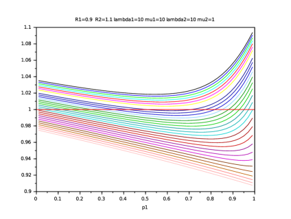
Figure 1: ${\cal R}_{1,2}$ as a function of $p_{1}$ in case A (each curve corresponds to a value of $p_{2}\in[0,1]$)

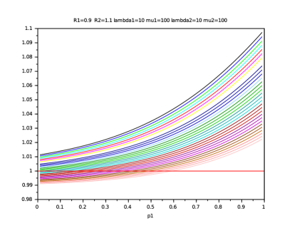
Figure 2: ${\cal R}_{1,2}$ as a function of $p_{1}$ in case B (each curve corresponds to a value of $p_{2}\in[0,1]$)

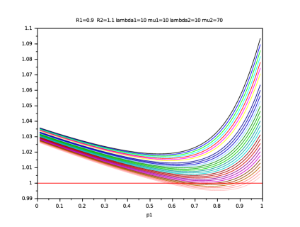
Figure 3: ${\cal R}_{1,2}$ as a function of $p_{1}$ in case C (each curve corresponds to a value of $p_{2}\in[0,1]$)

6 Conclusion

In this work, we have been able to provide an explicit expression of the reproduction number, although the model is in dimension $18$. This expression has allowed us to study its minimization with respect to the proportions of permanently resident populations in each patch. We discovered a trichotomy of cases, with some counter intuitive situations. In each case, it is always beneficial to have commuters traveling to a safer city where the transmission rate is lower. However, for the safer city, three situations occurs:

• either it is better to avoid commuting to the other city,

• or on the opposite encouraging commuting to the more risky city reduces the reproduction number,

• and in a third case there exists an optimal intermediate proportion of commuters of the safer city which minimizes the epidemic threshold.

In some sense, the permanently resident populations, which have been ignored in former modeling, can play an hidden role in an epidemic outbreak. This is illustrated on an example for which only right proportions of commuters (or permanently resident) avoid the outbreak. This suggests that counter-intuitive situations may also occur when considering networks with more than two nodes. The present study focuses on the reproduction number and how it can be reduced. The impacts of resident proportions on other epidemiological characteristics, such as the peak level or the finite size, may be the matter a future work. The extension of the present results to more general networks is also a future perspective.

References

• (1) Anderson, R.M. and May, R.M. Infectious Diseases of Humans, Oxford University, 1991.
• (2) Angulo, J.J, Takiguti, C.K, Pederneiras, C.A, Carvalho-de-Souza, A.M, Oliveira-de-Souza, M.C. and Megale, P. Identification of pattern and process in the spread of a contagious disease. Social Science & Medicine, 13D(3):183–9, 1979.
• (3) Arino, J., Jordan, R. and van den Driessche, P. Quarantine in a multi-species epidemic model with spatial dynamics. Mathematical Biosciences, 206(1), 46–60, 2007.
• (4) Arino, J. Diseases in Metapopulations. In Modeling and Dynamics of Infectious Diseases, World Scientific, 64–122, 2009.
• (5) Arino, J and van den Driessche, P. A multi-city epidemic model. Mathematical Population Studies, 10(3), 175–193, 2003.
• (6) Arino, J and van den Driessche, P. Disease spread in metapopulations. Fields Institute Communications, 48, 2006.
• (7) Berman, A. and Plemmons, R.J. Nonnegative Matrices in the Mathematical Sciences, SIAM, 1994.
• (8) Brunham, R. Core group theory: a central concept in STD epidemiology. Venereology, 10(1), 34–5, 8–9, 1997.
• (9) Citron, D.T., Guerra, C.A., Dolgert, A.J., Wu, S.L., Henry, J.M., Sánchez C, H. M. and Smith, D.L. Comparing metapopulation dynamics of infectious diseases under different models of human movement. Proceedings of the National Academy of Sciences, 118(18), e2007488118, 2021.
• (10) Chen, Y., Yan, M., and Xiang, Z., Transmission Dynamics of a Two-City SIR Epidemic Model with Transport-Related Infections. Journal of Applied Mathematics, ID 764278, 2014.
• (11) Clancy, D. Carrier-borne epidemic models incorporating population mobility. Mathematical Biosciences, 132(2), 185–204, 1996.
• (12) Colizza,V., Barrat, A., Barthelemy, M. and Vespignani, A. The role of the airline transportation network in the prediction and predictability of global epidemics. Proc. Natl. Acad. Sci. U.S.A. 103, 2015–2020, 2006.
• (13) Diekmann, O., Heesterbeek, H. and Britton T. Mathematical Tools for Understanding Infectious Disease Dynamics. Princeton University Press, 2013.
• (14) Diekmann, O., Heesterbeek, J.A.P. and Metz, J.A.J. On the definition and computation of the basic reproduction ratio R0 in models for infectious diseases in heterogeneous populations. Journal of Mathematical Biology, 28, 365–382 1990.
• (15) Diekmann, O., Heesterbeek, J.A.P. and Robert M.G., The construction of next-generation matrices for compartmental epidemic models. Journal of the Royal Society Interface, 7, 873–885, 2007.
• (16) Dhirasakdanon, T., Thieme, H.R. and Van Den Driessche, P. A sharp threshold for disease persistence in host metapopulations. Journal of Biological Dynamics, 1(4), 363–378, 2007.
• (17) Gao, D. How Does Dispersal Affect the Infection Size? SIAM Journal on Applied Mathematics, 80, 2144–2169, 2007.
• (18) Guo, H., Li, M. and Shuai, Z. Global stability of the endemic equilibrium of multigroup SIR epidemic models. Canadian Applied Mathematics Quarterly, 14(3), 259–284, 2006.
• (19) Hadeler, K.P. and Castillo-Chavez, C. A core group model for disease transmission, Mathematical Biosciences, 128 (1-2), 41–55, 1995.
• (20) Hanski, I. Metapopulation Ecology. Oxford University Press, 1999.
• (21) Iggidr, A., Sallet, G. and Tsanou, B. Global Stability Analysis of a Metapopulation SIS Epidemic Model. Mathematical Population Studies, 19(3), 115–129, 2012.
• (22) Keeling, M. J., Bjørnstad, O. N. and Grenfell, B. T. Metapopulation dynamics of infectious diseases. Chapter 17 in I. Hanski, and O. Gaggiotti (eds.). Ecology, Genetics, and Evolution of Metapopulations, Elsevier, 415–445, 2004.
• (23) Keeling, M.J. and Rohani, P. Estimating Spatial Coupling in Epidemiological Systems: a Mechanistic Approach. Ecology Letters, 5, 20–29, 2002.
• (24) Keeling, M.J. and Rohani, P. Modeling Infectious Diseases in Humans and Animals. Princeton University Press, 2007.
• (25) Kelly, M.R., Tien, J.H., Eisenberg, M.C and Lenhart, S. The impact of spatial arrangements on epidemic disease dynamics and intervention strategies. Journal of Biological Dynamics, 10, 222–49, 2016.
• (26) Kermack, W. and McKendrick, A. A contribution to the mathematical theory of epidemics.. Proceedings of the Royal Society, A 115, 700–721, 1927.
• (27) Knipl, D. A new approach for designing disease intervention strategies in metapopulation models. Journal of Biological Dynamics, 10(1), 71–94, 2016.
• (28) Li, J., Xiang, T. and He, L. Modeling epidemic spread in transportation networks: A review,. Journal of Traffic and Transportation Engineering, 8(2), 139–152, 2021.
• (29) Lipshtat, A., Alimi, R. and Ben-Horin, Y. Commuting in metapopulation epidemic modeling. Scientific Reports, 11, 15198, 2021.
• (30) Liu, X. and Stechlinski, P. Transmission dynamics of a switched multi-city model with transport-related infections. Nonlinear Analysis: Real World Applications, 14(1), 264–279, 2013.
• (31) MacArthur, R.H. and and Wilson, E.O. The Theory of Island Biogeography , Princeton University Press, 2001.
• (32) Mpolya, E.A., Yashima, K., Ohtsuki, H and Sasaki, A. Epidemic dynamics of a vector-borne disease on a villages-and-city star network with commuters. Journal of Theoretical Biology, 343, 120–26, 2014.
• (33) Murray, J.D. Mathematical Biology II: Spatial Models and Biomedical Applications. Springer, 2003.
• (34) Patil, R., Dave, R., Patel, H., Shah, V.M., Chakrabarti, D. and Bhatia, U. Assessing the interplay between travel patterns and SARS-CoV-2 outbreak in realistic urban setting. Applied Network Science 6, 4, 2021.
• (35) Ruan, Z., Wang, C., Ming Hui, P. and Liu, Z. Integrated travel network model for studying epidemics: Interplay between journeys and epidemic. Scientific Reports 5, 11401, 2015.
• (36) Sattenspiel, L. and Dietz, K. A structured epidemic model incorporating geographic mobility among regions. Mathematical Biosciences, 128 (1-2), 71–91, 1995.
• (37) Takeuchi, Y., Liu, X. and Cui, J. Global dynamics of SIS models with transport-related infection. Journal of Mathematical Analysis and Applications, 329(2), 1460-71, 2007.
• (38) Tocto-Erazo, M.R., Olmos-Liceaga, D. and Montoya-Laos, J.A. Effect of daily human movement on some characteristics of dengue dynamics. Mathematical Biosciences, 332, 108531, 2021.
• (39) van den Driessche, P. and Watmough, J. Reproduction numbers and sub-threshold endemic equilibria for compartmental models of disease transmission. Mathematical Biosciences, 180 (1-2), 29–48, 2002.
• (40) Vorotnikov, V.I Partial Stability and Control, Birkäuser, 1998.
• (41) Wang, W. and Mulone, G. Threshold of disease transmission in a patch environment. Journal of Mathematical Analysis and Applications, 285(1), 321–335, 2003.
• (42) Wang, W. and Zhao, X.Q. An epidemic model in a patchy environment. Mathematical Biosciences,190(1), 97–112, 2004.
• (43) Yin, Q., Wang, Z., Xia, C., Dehmer, M., Emmert-Streib, F. and Jin, Z. A novel epidemic model considering demographics and intercity commuting on complex dynamical networks. Applied Mathematics and Computation, 386, N. 125517, 2020.