Fully Stochastic Trust-Region Sequential Quadratic Programming for Equality-Constrained Optimization Problems

Abstract

We propose a trust-region stochastic sequential quadratic programming algorithm (TR-StoSQP) to solve nonlinear optimization problems with stochastic objectives and deterministic equality constraints. We consider a fully stochastic setting, where at each step a single sample is generated to estimate the objective gradient. The algorithm adaptively selects the trust-region radius and, compared to the existing line-search StoSQP schemes, allows us to utilize indefinite Hessian matrices (i.e., Hessians without modification) in SQP subproblems. As a trust-region method for constrained optimization, our algorithm must address an infeasibility issue — the linearized equality constraints and trust-region constraints may lead to infeasible SQP subproblems. In this regard, we propose an adaptive relaxation technique to compute the trial step, consisting of a normal step and a tangential step. To control the lengths of these two steps while ensuring a scale-invariant property, we adaptively decompose the trust-region radius into two segments, based on the proportions of the rescaled feasibility and optimality residuals to the rescaled full KKT residual. The normal step has a closed form, while the tangential step is obtained by solving a trust-region subproblem, to which a solution ensuring the Cauchy reduction is sufficient for our study. We establish a global almost sure convergence guarantee for TR-StoSQP, and illustrate its empirical performance on both a subset of problems in the CUTEst test set and constrained logistic regression problems using data from the LIBSVM collection.

1 Introduction

We consider the constrained stochastic optimization problem:

$$\min_{{\bm{x}}\in\mathbb{R}^{d}}\;f({\bm{x}})=\mathbb{E}[F({\bm{x}};\xi)],\quad\text{s.t.}\;\;c({\bm{x}})={\bm{0}},$$ (1)

where $f:\mathbb{R}^{d}\rightarrow\mathbb{R}$ is a stochastic objective with $F(\cdot;\xi)$ being one of its realizations, $c:\mathbb{R}^{d}\rightarrow\mathbb{R}^{m}$ are deterministic equality constraints, $\xi$ is a random variable following the distribution ${\mathcal{P}}$, and the expectation $\mathbb{E}[\cdot]$ is taken over the randomness of $\xi$. Problem (1) appears in various applications including constrained deep neural networks (Chen et al., 2018), constrained maximum likelihood estimation (Dupacova and Wets, 1988), optimal control (Birge, 1997), PDE-constrained optimization (Rees et al., 2010), and network optimization (Bertsekas, 1998).

There are numerous methods for solving constrained optimization problems with deterministic objectives. Among them, sequential quadratic programming (SQP) methods are one of the leading approaches and are effective for both small and large problems. When the objective is stochastic, some stochastic SQP (StoSQP) methods have been proposed recently (Berahas et al., 2021b; Na et al., 2022a; Berahas et al., 2021a; Na et al., 2021; Curtis et al., 2021b; Berahas et al., 2022b). That body of literature considers the following two different setups for modeling the objective.

The first setup is called the random model setup (Chen et al., 2017), where samples with adaptive batch sizes are generated in each iteration to estimate the objective model (e.g., objective value and gradient). The algorithms under this setup often require the estimated objective model to satisfy certain adaptive accuracy conditions with a fixed probability in each iteration. Under this setup, Na et al. (2022a) proposed an StoSQP algorithm for (1), which adopts a stochastic line search procedure with an exact augmented Lagrangian merit function to select the stepsize. Subsequently, Na et al. (2021) further enhanced the designs and arguments in Na et al. (2022a) and developed an active-set StoSQP method to enable inequality constraints; and Berahas et al. (2022b) considered a finite-sum objective and accelerated StoSQP by applying the SVRG technique (Johnson and Zhang, 2013), which, however, requires one to periodically compute the full objective gradient. Also, Berahas et al. (2022a) introduced a norm test condition for StoSQP to adaptively select the batch sizes.

The second setup is called the fully stochastic setup (Curtis and Shi, 2020), where a single sample is generated in each iteration to estimate the objective model. Under this setup, a prespecified sequence is often required as an input to assist with the step selection. For example, Berahas et al. (2021b) designed an StoSQP scheme that uses a random projection procedure to select the stepsize. The projection procedure uses a prespecified sequence $\{\beta_{k}\}$, together with the estimated Lipschitz constants of the objective gradient and constraint Jacobian, to construct a projection interval in each iteration. A random quantity is then computed and projected into the interval to decide the stepsize, which ensures a sufficient reduction on the $\ell_{1}$ merit function. Following from Berahas et al. (2021b), some algorithmic and theoretical improvements have been reported: Berahas et al. (2021a) dealt with rank-deficient Jacobians; Curtis et al. (2021b) solved Newton systems inexactly; Curtis et al. (2021a) analyzed the worst-case sample complexity; and Na and Mahoney (2022) established the local rate and performed statistical inference for the method in Berahas et al. (2021b).

The existing StoSQP algorithms converge globally either in expectation or almost surely, and enjoy promising empirical performance under favorable settings. However, there are three limitations that motivate our study. First, the algorithms are all line-search-based; that is, a search direction is first computed by solving an SQP subproblem, and then a stepsize is selected, either by random projection or by stochastic line search along the direction. However, it is observed that for deterministic problems, computing the search direction and selecting the stepsize jointly, as is done in trust-region methods, can lead to better performance in some cases (Nocedal and Wright, 2006, Chapter 4). Second, to make SQP subproblems solvable, the existing schemes require the approximation of the Lagrangian Hessian to be positive definite in the null space of constraint Jacobian. Such a condition is common in the SQP literature (Boggs and Tolle, 1995; Nocedal and Wright, 2006), while it is often achieved by Hessian modification, which excludes promising choices of the Hessian matrices, such as the unperturbed (stochastic) Hessian of the Lagrangian. Third, to show global convergence, the existing literature requires the random merit parameter to be not only stabilized, but also sufficiently large (or small, depending on the context) with an unknown threshold. To achieve the latter goal, Na et al. (2022a, 2021) imposed an adaptive condition on the feasibility error when selecting the merit parameter, while Berahas et al. (2021a, b, 2022b); Curtis et al. (2021b) imposed a symmetry condition on the noise distribution. In contrast, deterministic SQP schemes only require the stability of the merit parameter (see Boggs and Tolle (1995) and references therein).

In this paper, we consider the fully stochastic setup and design a trust-region stochastic SQP (TR-StoSQP) method to address the above limitations. As a trust-region method, TR-StoSQP computes the search direction and stepsize jointly, and, unlike line-search-based methods, it avoids Hessian modifications in formulating SQP subproblems. Thus, it can explore negative curvature directions of the Hessian. Further, our analysis only relies on the stability of the merit parameter (of the $\ell_{2}$ merit function), which is consistent with deterministic SQP schemes. The design of TR-StoSQP is inspired by a stochastic trust-region method for solving unconstrained problems reported in Curtis and Shi (2020), which improves the authors’ prior design in Curtis et al. (2019) from using linear model to quadratic model to approximate the objective function. As in Curtis and Shi (2020), our method inputs a user-specified radius-related sequence $\{\beta_{k}\}$ to generate the trust-region radius at each step. Beyond this similarity, our scheme differs from Curtis and Shi (2020) in several aspects.

First, it is known that trust-region methods for constrained optimization are bothered by the infeasibility issue — the linearized constraints and trust-region constraints may have an empty intersection, leading to an infeasible SQP subproblem. While some literature on trust-region SQP has been proposed to address this issue (Celis et al., 1984; Vardi, 1985; Byrd et al., 1987; Omojokun, 1989), we develop a novel adaptive relaxation technique to compute the trial step, which preserves a scale-invariant property and can be further adapted to our stochastic setup. In particular, we decompose the trial step into a normal step and a tangential step. Then, we control the lengths of the two steps by decomposing the trust-region radius into two segments adaptively, based on the proportions of the rescaled estimated feasibility and optimality residuals to the rescaled full KKT residual. Compared to the existing relaxation techniques, our relaxation technique does not require any tuning parameters. See Section 2 for details.

Second, in TR-StoSQP, we properly compute some control parameters using known or estimable quantities. By the computation, we no longer need to tune the other two input parameter sequences as in Curtis and Shi (2020) (i.e., $\{\gamma_{1,k},\gamma_{2,k}\}$ in their notation), except to tune the input radius-related sequence $\{\beta_{k}\}$. Further, we use the control parameters to adjust the input sequence $\{\beta_{k}\}$ when computing the trust-region radius, so that $\{\beta_{k}\}\subseteq(0,\beta_{\max}]$ with any $\beta_{\max}>0$ is sufficient for our convergence analysis. Our design simplifies the one in Curtis and Shi (2020), where there are three parameter sequences to tune whose conditions are highly coupled (see Curtis and Shi, 2020, Lemma 4.5). In addition, as the authors stated, Curtis and Shi (2020) rescaled the Hessian matrix based on the input $\{\gamma_{1,k}\}$, which is not ideal (because the rescaling step modifies the curvature information of the Hessian). We have removed this step in our design.

To our knowledge, TR-StoSQP is the first trust-region SQP algorithm for solving constrained optimization problems under fully stochastic setup. With a stabilized merit parameter, we establish the global convergence property of TR-StoSQP. In particular, we show that (i) when $\beta_{k}=\beta$, $\forall k\geq 0$, the expectation of weighted averaged KKT residuals converges to a neighborhood around zero; (ii) when $\beta_{k}$ decays properly such that $\sum\beta_{k}=\infty$ and $\sum\beta_{k}^{2}<\infty$, the KKT residuals converge to zero almost surely. These results are similar to the ones for unconstrained and constrained problems established under fully stochastic setup in Berahas et al. (2021b, a); Curtis et al. (2021b); Curtis and Shi (2020). However, we have weaker conditions on the objective gradient noise (e.g., we consider a growth condition) and on the sequence $\beta_{k}$ (e.g., we only require $\beta_{k}\leq\beta_{\max}$). See the discussions after Theorem 4.9 and Theorem 4.11 for more details. We also note that a recent paper (Sun and Nocedal, 2023) studied a noisy trust-region method for unconstrained deterministic optimization. In that method, the value and gradient of the objective are evaluated with bounded deterministic noise. The authors showed that the trust-region iterates visit a neighborhood of the stationarity infinitely often, with the radius proportional to the noise magnitude. Given the significant differences between stochastic and deterministic problems, and between constrained and unconstrained problems, our algorithm design and analysis are quite different from Sun and Nocedal (2023). That said, when studying the stability of the merit parameter, we follow existing literature (e.g., Berahas et al., 2021b, a; Na et al., 2022a) and also require the bounded gradient noise condition. We implement TR-StoSQP on a subset of problems in the CUTEst test set and on constrained logistic regression problems using data from the LIBSVM collection. Numerical results demonstrate the promising performance of our method.

Notation. We use $\|\cdot\|$ to denote the $\ell_{2}$ norm for vectors and the operator norm for matrices. $I$ denotes the identity matrix and ${\bm{0}}$ denotes the zero matrix (or vector). Their dimensions are clear from the context. We let $G({\bm{x}})=\nabla^{T}c({\bm{x}})\in\mathbb{R}^{m\times d}$ be the Jacobian matrix of the constraints and $P({\bm{x}})=I-G^{T}({\bm{x}})[G({\bm{x}})G^{T}({\bm{x}})]^{-1}G({\bm{x}})$ be the projection matrix to the null space of $G({\bm{x}})$. We use ${\bar{g}}({\bm{x}})=\nabla F({\bm{x}};\xi)$ to denote an estimate of $\nabla f({\bm{x}})$, and use $\bar{(\cdot)}$ to denote stochastic quantities.

Structure of the paper. We introduce the adaptive relaxation technique in Section 2. We propose the trust-region stochastic SQP (TR-StoSQP) algorithm in Section 3 and establish its global convergence guarantee in Section 4. Numerical experiments are presented in Section 5 and conclusions are presented in Section 6. Some additional analyses are provided in Appendix A.

2 Adaptive Relaxation for Deterministic Setup

Lagrangian of Problem (1) is ${\mathcal{L}}({\bm{x}},{\bm{\lambda}})=f({\bm{x}})+{\bm{\lambda}}^{T}c({\bm{x}})$, where ${\bm{\lambda}}\in\mathbb{R}^{m}$ is the dual vector. Finding a first-order stationary point of (1) is equivalent to finding a pair $({\bm{x}}^{*},{\bm{\lambda}}^{*})$ such that

$$\nabla{\mathcal{L}}({\bm{x}}^{*},{\bm{\lambda}}^{*})=\begin{pmatrix}\nabla_{\bm{x}}{\mathcal{L}}({\bm{x}}^{*},{\bm{\lambda}}^{*})\\ \nabla_{{\bm{\lambda}}}{\mathcal{L}}({\bm{x}}^{*},{\bm{\lambda}}^{*})\end{pmatrix}=\begin{pmatrix}\nabla f({\bm{x}}^{*})+G^{T}({\bm{x}}^{*}){\bm{\lambda}}^{*}\\ c({\bm{x}}^{*})\end{pmatrix}=\begin{pmatrix}{\bm{0}}\\ {\bm{0}}\end{pmatrix}.$$

We call $\|\nabla_{\bm{x}}{\mathcal{L}}({\bm{x}},{\bm{\lambda}})\|$ the optimality residual, $\|\nabla_{\bm{\lambda}}{\mathcal{L}}({\bm{x}},{\bm{\lambda}})\|$ (i.e., $\|c({\bm{x}})\|$) the feasibility residual, and $\|\nabla{\mathcal{L}}({\bm{x}},{\bm{\lambda}})\|$ the KKT residual. Given ${\bm{x}}_{k}$ in the $k$-th iteration, we denote $\nabla f_{k}=\nabla f({\bm{x}}_{k})$, $c_{k}=c({\bm{x}}_{k})$, $G_{k}=G({\bm{x}}_{k})$, etc.

2.1 Preliminaries

Given the iterate ${\bm{x}}_{k}$ and the trust-region radius $\Delta_{k}$ in the $k$-th iteration, we compute an approximation $B_{k}$ of the Lagrangian Hessian $\nabla^{2}_{{\bm{x}}}{\mathcal{L}}_{k}$, and aim to obtain the trial step $\Delta{\bm{x}}_{k}$ by solving a trust-region SQP subproblem

$$\min_{\Delta{\bm{x}}\in\mathbb{R}^{d}}\ \frac{1}{2}\Delta{\bm{x}}^{T}B_{k}\Delta{\bm{x}}+\nabla f_{k}^{T}\Delta{\bm{x}},\;\quad\text{s.t.}\;\;c_{k}+G_{k}\Delta{\bm{x}}={\bm{0}},\;\|\Delta{\bm{x}}\|\leq\Delta_{k}.$$ (2)

However, if $\{\Delta{\bm{x}}\in\mathbb{R}^{d}:c_{k}+G_{k}\Delta{\bm{x}}={\bm{0}}\}\cap\{\Delta{\bm{x}}\in\mathbb{R}^{d}:\|\Delta{\bm{x}}\|\leq\Delta_{k}\}=\emptyset$, then (2) does not have a feasible point. This infeasibility issue happens when the radius $\Delta_{k}$ is too short. To resolve this issue, one should not enlarge $\Delta_{k}$, which would make the trust-region constraint useless and violate the spirit of the trust-region scheme. Instead, one should relax the linearized constraint $c_{k}+G_{k}\Delta{\bm{x}}={\bm{0}}$.

Before introducing our adaptive relaxation technique, we review some classical relaxation techniques. To start, Celis et al. (1984) relaxed the linearized constraint by $\|c_{k}+G_{k}\Delta{\bm{x}}\|\leq\theta_{k}$ with $\theta_{k}=\|c_{k}+G_{k}\Delta{\bm{x}}_{k}^{CP}\|$, where $\Delta{\bm{x}}_{k}^{CP}$ is the Cauchy point (i.e., the best steepest descent step) of the following problem:

$$\min_{\Delta{\bm{x}}\in\mathbb{R}^{d}}\ \|c_{k}+G_{k}\Delta{\bm{x}}\|\;\quad\text{s.t.}\quad\|\Delta{\bm{x}}\|\leq\Delta_{k}.$$ (3)

However, since after the relaxation one has to minimize a quadratic function over the intersection of two ellipsoids $\|c_{k}+G_{k}\Delta{\bm{x}}\|\leq\theta_{k}$ and $\|\Delta{\bm{x}}\|\leq\Delta_{k}$, the resulting SQP subproblem tends to be expensive to solve. See Yuan (1990) for some insights into the difficulty, and see Yuan (1991); Zhang (1992) for the methods for positive definite $B_{k}$. Alternatively, Vardi (1985) relaxed the linearized constraint by $\gamma_{k}c_{k}+G_{k}\Delta{\bm{x}}={\bm{0}}$, with $\gamma_{k}\in(0,1]$ chosen to make the trust-region constraint of (2) inactive. However, Vardi (1985) only showed the existence of an extremely small $\gamma_{k}$, and it did not provide a practical way to choose it. Subsequently, Byrd et al. (1987) refined the relaxation technique of Vardi (1985) by a step decomposition. At the $k$-th step, Byrd et al. (1987) decomposed the trial step $\Delta{\bm{x}}_{k}$ into a normal step $\bm{w}_{k}\in\text{im}(G_{k}^{T})$ and a tangential step $\bm{t}_{k}\in\text{ker}(G_{k})$, denoted as $\Delta{\bm{x}}_{k}=\bm{w}_{k}+\bm{t}_{k}$. By the constraint $\gamma_{k}c_{k}+G_{k}\Delta{\bm{x}}_{k}={\bm{0}}$, the normal step has a closed form as (suppose $G_{k}$ has full row rank)

$$\bm{w}_{k}\coloneqq\gamma_{k}{\bm{v}}_{k}\coloneqq-\gamma_{k}\cdot G_{k}^{T}[G_{k}G_{k}^{T}]^{-1}c_{k},$$ (4)

and the tangential step is expressed as $\bm{t}_{k}=Z_{k}{\bm{u}}_{k}$ for a vector ${\bm{u}}_{k}\in\mathbb{R}^{d-m}$. Here, the columns of $Z_{k}\in\mathbb{R}^{d\times(d-m)}$ form the bases of $\text{ker}(G_{k})$. Byrd et al. (1987) proposed to choose $\gamma_{k}$ such that $\theta\Delta_{k}\leq\|\bm{w}_{k}\|\leq\Delta_{k}$ for a tuning parameter $\theta\in(0,1)$, and solve ${\bm{u}}_{k}$ from

$$\min_{{\bm{u}}\in\mathbb{R}^{d-m}}\;\frac{1}{2}{\bm{u}}^{T}Z_{k}^{T}B_{k}Z_{k}{\bm{u}}+(\nabla f_{k}+B_{k}\bm{w}_{k})^{T}Z_{k}{\bm{u}}\;\quad\text{s.t.}\;\;\|{\bm{u}}\|^{2}\leq\Delta_{k}^{2}-\|\bm{w}_{k}\|^{2}.$$ (5)

Furthermore, Omojokun (1989) combined the techniques of Celis et al. (1984) and Byrd et al. (1987); it solved the normal step $\bm{w}_{k}$ from Problem (3) by replacing the constraint $\|\Delta{\bm{x}}\|\leq\Delta_{k}$ with $\|\Delta{\bm{x}}\|\leq\theta\Delta_{k}$ for some $\theta\in(0,1)$; and it solved the tangential step $\bm{t}_{k}=Z_{k}{\bm{u}}_{k}$ from Problem (5). We note that the solution of (3) is naturally a normal step (i.e., lies in $\text{im}(G_{k}^{T})$), because any directions in $\text{ker}(G_{k})$ do not change the objective in (3).

Although the methods in Byrd et al. (1987); Omojokun (1989) allow one to employ Cauchy points for trust-region subproblems, they lack guidance for selecting the user-specified parameter $\theta$, which controls the lengths of the normal and tangential steps. In fact, an inappropriate parameter $\theta$ may make either step conservative and further affect the effectiveness of the algorithm. As we show in (9) and (10) later, the normal step relates to the reduction of the feasibility residual, while the tangential step relates to the reduction of the optimality residual. We hope the two steps scale properly so that the model reduction achieved by $\Delta{\bm{x}}_{k}$ is large enough. To that end, we propose an adaptive relaxation technique, which is parameter-free in step decomposition compared to Vardi (1985); Byrd et al. (1987); Omojokun (1989).

2.2 Our adaptive relaxation technique

We introduce our parameter-free relaxation procedure. Same as Byrd et al. (1987), we relax the linearized constraint in (2) by $\gamma_{k}c_{k}+G_{k}\Delta{\bm{x}}={\bm{0}}$ with $\gamma_{k}$ defined later, and decompose the trial step by $\Delta{\bm{x}}_{k}=\bm{w}_{k}+\bm{t}_{k}$. The normal step $\bm{w}_{k}$ is given by (4), and the tangential step is of the form $\bm{t}_{k}=Z_{k}{\bm{u}}_{k}$.

To control the lengths of the two steps while ensuring a scale-invariant property (cf. Remark 2.2), let us define the rescaled optimality vector $\nabla_{{\bm{x}}}{\mathcal{L}}^{RS}_{k}\coloneqq\nabla_{{\bm{x}}}{\mathcal{L}}_{k}/\|B_{k}\|$, the feasibility vector $c^{RS}_{k}\coloneqq c_{k}/\|G_{k}\|$, and the KKT vector $\nabla{\mathcal{L}}^{RS}_{k}\coloneqq(\nabla_{{\bm{x}}}{\mathcal{L}}^{RS}_{k},c^{RS}_{k})$. (One alternative choice of the rescaled feasibility vector can be ${\bm{v}}_{k}=G_{k}^{T}[G_{k}G_{k}^{T}]^{-1}c_{k}$.) Then, we adaptively decompose the trust-region radius $\Delta_{k}$ into two segments, based on the proportions of the rescaled feasibility and optimality residuals to the rescaled full KKT residual. We let

$$\breve{\Delta}_{k}=\frac{\|c_{k}^{RS}\|}{\|\nabla{\mathcal{L}}_{k}^{RS}\|}\cdot\Delta_{k}\quad\quad\text{ and }\quad\quad\widetilde{\Delta}_{k}=\frac{\|\nabla_{{\bm{x}}}{\mathcal{L}}_{k}^{RS}\|}{\|\nabla{\mathcal{L}}_{k}^{RS}\|}\cdot\Delta_{k}.$$ (6)

It is implicitly assumed that $\|B_{k}\|,\|G_{k}\|,\|\nabla{\mathcal{L}}_{k}\|\neq 0$, which is quite reasonable for SQP methods. We let $\breve{\Delta}_{k}$ control the length of the normal step $\bm{w}_{k}$ and $\widetilde{\Delta}_{k}$ control the length of the tangential step $\bm{t}_{k}$. Specifically, we define $\gamma_{k}$ as (recall ${\bm{v}}_{k}$ is defined in (4))

$$\gamma_{k}\coloneqq\min\{\breve{\Delta}_{k}/\|{\bm{v}}_{k}\|,1\}$$ (7)

so that $\|\bm{w}_{k}\|=\gamma_{k}\|{\bm{v}}_{k}\|\leq\breve{\Delta}_{k}$, and we compute ${\bm{u}}_{k}$ by solving

$$\min_{{\bm{u}}\in\mathbb{R}^{d-m}}\ m({\bm{u}})\coloneqq\frac{1}{2}{\bm{u}}^{T}Z_{k}^{T}B_{k}Z_{k}{\bm{u}}+(\nabla f_{k}+B_{k}\bm{w}_{k})^{T}Z_{k}{\bm{u}}\;\quad\text{ s.t. }\;\;\|{\bm{u}}\|\leq\widetilde{\Delta}_{k}.$$ (8)

When ${\bm{v}}_{k}=0$ (i.e., $c_{k}={\bm{0}}$), there is no need to choose $\gamma_{k}$ and we set $\Delta{\bm{x}}_{k}=Z_{k}{\bm{u}}_{k}$. Problem (8) is a trust-region subproblem that appears in unconstrained optimization. In our analysis, we only require a vector ${\bm{u}}_{k}$ that reduces $m({\bm{u}})$ by at least as much as the Cauchy point, which takes the direction of $-Z_{k}^{T}(\nabla f_{k}+B_{k}\bm{w}_{k})$ and minimizes $m({\bm{u}})$ within the trust region (Nocedal and Wright, 2006, Algorithm 4.2). Such a reduction requirement can be achieved by various methods, including finding the exact solution or applying the dogleg or two-dimensional subspace minimization methods (Nocedal and Wright, 2006).

The following result provides a bound on the reduction in $m({\bm{u}})$ that is different from the standard analysis of the Cauchy point; (e.g., Nocedal and Wright, 2006, Lemma 4.3).

Lemma 2.1.

Let ${\bm{u}}_{k}$ be an approximate solution to (8) that reduces the objective $m({\bm{u}})$ by at least as much as the Cauchy point. For all $k\geq 0$, we have

$$m({\bm{u}}_{k})-m({\bm{0}})=\frac{1}{2}{\bm{u}}_{k}^{T}Z_{k}^{T}B_{k}Z_{k}{\bm{u}}_{k}+(\nabla f_{k}+B_{k}\bm{w}_{k})^{T}Z_{k}{\bm{u}}_{k}\\ \leq-\|Z_{k}^{T}(\nabla f_{k}+B_{k}\bm{w}_{k})\|\widetilde{\Delta}_{k}+\frac{1}{2}\|B_{k}\|\widetilde{\Delta}_{k}^{2}.$$

Proof.

Let ${\bm{u}}_{k}^{CP}$ denote the Cauchy point. Since $m({\bm{u}}_{k})\leq m({\bm{u}}_{k}^{CP})$, it suffices to analyze the reduction achieved by ${\bm{u}}_{k}^{CP}$. By the formula of ${\bm{u}}_{k}^{CP}$ in (Nocedal and Wright, 2006, (4.12)), we know that if $\|Z_{k}^{T}(\nabla f_{k}+B_{k}\bm{w}_{k})\|^{3}\leq\widetilde{\Delta}_{k}(\nabla f_{k}+B_{k}\bm{w}_{k})^{T}Z_{k}Z_{k}^{T}B_{k}Z_{k}Z_{k}^{T}(\nabla f_{k}+B_{k}\bm{w}_{k})$, then ${\bm{u}}_{k}^{CP}=-\|Z_{k}^{T}(\nabla f_{k}+B_{k}\bm{w}_{k})\|^{2}/(\nabla f_{k}+B_{k}\bm{w}_{k})^{T}Z_{k}Z_{k}^{T}B_{k}Z_{k}Z_{k}^{T}(\nabla f_{k}+B_{k}\bm{w}_{k})\cdot Z_{k}^{T}(\nabla f_{k}+B_{k}\bm{w}_{k})$. In this case, using $\|Z_{k}\|\leq 1$, we have

$$m({\bm{u}}_{k}^{CP})-m({\bm{0}})=\frac{1}{2}(Z_{k}{\bm{u}}_{k}^{CP})^{T}B_{k}Z_{k}{\bm{u}}_{k}^{CP}+(\nabla f_{k}+B_{k}\bm{w}_{k})^{T}Z_{k}{\bm{u}}_{k}^{CP}\\ =-\frac{1}{2}\frac{\|Z_{k}^{T}(\nabla f_{k}+B_{k}\bm{w}_{k})\|^{4}}{(\nabla f_{k}+B_{k}\bm{w}_{k})^{T}Z_{k}Z_{k}^{T}B_{k}Z_{k}Z_{k}^{T}(\nabla f_{k}+B_{k}\bm{w}_{k})}\leq-\frac{1}{2}\frac{\|Z_{k}^{T}(\nabla f_{k}+B_{k}\bm{w}_{k})\|^{2}}{\|B_{k}\|}.$$

Otherwise, ${\bm{u}}_{k}^{CP}=-\widetilde{\Delta}_{k}/\|Z_{k}^{T}(\nabla f_{k}+B_{k}\bm{w}_{k})\|\cdot Z_{k}^{T}(\nabla f_{k}+B_{k}\bm{w}_{k})$. In this case, we have

$$m({\bm{u}}_{k}^{CP}) -m({\bm{0}})=\frac{1}{2}(Z_{k}{\bm{u}}_{k}^{CP})^{T}B_{k}Z_{k}{\bm{u}}_{k}^{CP}+(\nabla f_{k}+B_{k}\bm{w}_{k})^{T}Z_{k}{\bm{u}}_{k}^{CP}$$

$$=\frac{(\nabla f_{k}+B_{k}\bm{w}_{k})^{T}Z_{k}Z_{k}^{T}B_{k}Z_{k}Z_{k}^{T}(\nabla f_{k}+B_{k}\bm{w}_{k})}{2\|Z_{k}^{T}(\nabla f_{k}+B_{k}\bm{w}_{k})\|^{2}}\widetilde{\Delta}_{k}^{2}-\|Z_{k}^{T}(\nabla f_{k}+B_{k}\bm{w}_{k})\|\widetilde{\Delta}_{k}$$

$$\leq\frac{1}{2}\|B_{k}\|\widetilde{\Delta}_{k}^{2}-\|Z_{k}^{T}(\nabla f_{k}+B_{k}\bm{w}_{k})\|\widetilde{\Delta}_{k}.$$

Combining the above two cases, we have

$$m({\bm{u}}_{k}^{CP})-m({\bm{0}})\leq-\min\left\{-\frac{\|B_{k}\|\widetilde{\Delta}_{k}^{2}}{2}+\|Z_{k}^{T}(\nabla f_{k}+B_{k}\bm{w}_{k})\|\widetilde{\Delta}_{k},\;\frac{\|Z_{k}^{T}(\nabla f_{k}+B_{k}\bm{w}_{k})\|^{2}}{2\|B_{k}\|}\right\}.$$

Using the fact that

$$-\frac{1}{2}\|B_{k}\|\widetilde{\Delta}_{k}^{2}+\|Z_{k}^{T}(\nabla f_{k}+B_{k}\bm{w}_{k})\|\widetilde{\Delta}_{k}\\ =-\frac{\|B_{k}\|}{2}\left(\widetilde{\Delta}_{k}-\frac{\|Z_{k}^{T}(\nabla f_{k}+B_{k}\bm{w}_{k})\|}{\|B_{k}\|}\right)^{2}+\frac{\|Z_{k}^{T}(\nabla f_{k}+B_{k}\bm{w}_{k})\|^{2}}{2\|B_{k}\|}\leq\frac{\|Z_{k}^{T}(\nabla f_{k}+B_{k}\bm{w}_{k})\|^{2}}{2\|B_{k}\|},$$

we complete the proof. ∎

It is easy to see that our relaxation technique indeed results in a trial step that lies in the trust region. We have (noting that $\|Z_{k}\|\leq 1$)

$$\|\Delta{\bm{x}}_{k}\|^{2}=\|\bm{w}_{k}\|^{2}+\|\bm{t}_{k}\|^{2}=(\gamma_{k}\|{\bm{v}}_{k}\|)^{2}+\|{\bm{u}}_{k}\|^{2}\stackrel{{\scriptstyle\eqref{eq:Sto_gamma_k},\eqref{eq:Sto_tangential_step}}}{{\leq}}\breve{\Delta}_{k}^{2}+\widetilde{\Delta}_{k}^{2}\stackrel{{\scriptstyle\eqref{eq:breve and tilde_delta_k}}}{{=}}\Delta_{k}^{2}.$$

Recalling from (4) that $\bm{w}_{k}=-\gamma_{k}G_{k}^{T}[G_{k}G_{k}^{T}]^{-1}c_{k}$, we know $c_{k}+G_{k}\bm{w}_{k}=(1-\gamma_{k})c_{k}$. Thus, we have

$$\|c_{k}+G_{k}\Delta{\bm{x}}_{k}\|-\|c_{k}\|=\|c_{k}+G_{k}\bm{w}_{k}\|-\|c_{k}\|=-\gamma_{k}\|c_{k}\|\leq 0,$$ (9)

where the strict inequality holds as long as $c_{k}\neq{\bm{0}}$. This inequality suggests that the normal step $\bm{w}_{k}$ helps to reduce the feasibility residual. Furthermore, when we define the least-squares Lagrangian multiplier as $\bm{\lambda}_{k}=-G_{k}^{T}[G_{k}G_{k}^{T}]\nabla f_{k}$, we have $P_{k}\nabla f_{k}=\nabla_{{\bm{x}}}{\mathcal{L}}_{k}$. Noting that $Z_{k}Z_{k}^{T}=P_{k}$, $P_{k}^{2}=P_{k}$ and $Z_{k}^{T}Z_{k}=I$, we obtain

$$\|Z_{k}^{T}(\nabla f_{k}+B_{k}\bm{w}_{k})\|^{2} =(\nabla f_{k}+B_{k}\bm{w}_{k})^{T}Z_{k}Z_{k}^{T}(\nabla f_{k}+B_{k}\bm{w}_{k})$$

$$=(\nabla f_{k}+B_{k}\bm{w}_{k})^{T}P_{k}^{2}(\nabla f_{k}+B_{k}\bm{w}_{k})=\|\nabla_{{\bm{x}}}{\mathcal{L}}_{k}+P_{k}B_{k}\bm{w}_{k}\|^{2}.$$

Thus, the conclusion of Lemma 2.1 can be rewritten as

$$m({\bm{u}}_{k})-m({\bm{0}})\leq-\|\nabla_{{\bm{x}}}{\mathcal{L}}_{k}+P_{k}B_{k}\bm{w}_{k}\|\widetilde{\Delta}_{k}+\frac{1}{2}\|B_{k}\|\widetilde{\Delta}_{k}^{2},$$ (10)

indicating that the tangential step relates to the reduction of the optimality residual.

To end this section, we would like to link our relaxation technique with those in Byrd et al. (1987); Omojokun (1989) in Remark 2.2.

Remark 2.2.

In our method, we define rescaled residuals $\|\nabla_{{\bm{x}}}{\mathcal{L}}^{RS}_{k}\|$, $\|c^{RS}_{k}\|$, $\|\nabla{\mathcal{L}}^{RS}_{k}\|$, and adaptively decompose the radius based on the proportions of these rescaled residuals (cf. (6)). We have two motivations: (i) the relation of the normal and tangential steps to the feasibility and optimality residuals; (ii) a scale-invariant property. We explain as follows.

Seeing from (9) and (10), the normal step relates to the reduction of the feasibility residual, while the tangential step relates to the reduction of the optimality residual. When the proportion of the feasibility residual is larger than that of the optimality residual, decreasing the feasibility residual is more important. As a result, we assign a larger trust-region radius to the normal step to achieve a larger reduction in the feasibility residual. Otherwise, we assign a larger radius to the tangential step to achieve a larger reduction in the optimality residual. In comparison, Byrd et al. (1987); Omojokun (1989) rely on a fixed proportion constant $\theta\in(0,1)$, making their approach less adaptive than ours.

On the other hand, we note that Byrd et al. (1987); Omojokun (1989) enjoy a nice scale-invariant property: given the radius $\Delta_{k}$, the trial step $\Delta{\bm{x}}_{k}$ is invariant when the constraints $c$ and/or the objective $f$ are rescaled by a (positive) scalar. Note that if $f$ (or $c$) is rescaled by a positive scalar, the Lagrangian Hessian (or the constraints Jacobian) will be rescaled by the same scalar. To preserve the invariance property, we decompose $\Delta_{k}$ using the rescaled residuals, as opposed to the original residuals $\|\nabla_{{\bm{x}}}\mathcal{L}_{k}\|$ and $\|c_{k}\|$; the latter can never be scale-invariant.

In the next section, we move to the fully stochastic setup and utilize the proposed relaxation scheme to design an StoSQP algorithm for (1). We will also discuss how to use the relaxation in Byrd et al. (1987) to design a StoSQP method.

3 A Trust-Region Stochastic SQP Algorithm

From now on, we replace the deterministic gradient $\nabla f({\bm{x}})$ by its stochastic estimate ${\bar{g}}({\bm{x}})=\nabla F({\bm{x}};\xi)$. Similar to Section 2, we denote ${\bar{g}}_{k}={\bar{g}}({\bm{x}}_{k})$ and define the estimated KKT residual as $\|{\bar{\nabla}}\mathcal{L}_{k}\|=\|({\bar{\nabla}}_{\bm{x}}\mathcal{L}_{k},c_{k})\|$ with ${\bar{\nabla}}_{\bm{x}}\mathcal{L}_{k}={\bar{g}}_{k}+G_{k}^{T}{\bm{\lambda}}_{k}$.

We summarize the proposed TR-StoSQP algorithm in Algorithm 1, and introduce the algorithm details as follows. In the $k$-th iteration, we are given the iterate ${\bm{x}}_{k}$, two fixed scalars $\zeta>0$ and $\delta\geq 0$, and the parameters $(\beta_{k},L_{\nabla f,k},L_{G,k},{\bar{\mu}}_{k-1})$. Here, $\beta_{k}\in(0,\beta_{\max}]$ with upper bound $\beta_{\max}>0$ is the input radius-related parameter; $L_{\nabla f,k}$ and $L_{G,k}$ are the (estimated) Lipschitz constants of $\nabla f({\bm{x}})$ and $G({\bm{x}})$ (in practice, they can be estimated by standard procedures in Curtis and Robinson (2018); Berahas et al. (2021b)); and ${\bar{\mu}}_{k-1}$ is the merit parameter of the $\ell_{2}$ merit function obtained after the $(k-1)$-th iteration. With these parameters, we proceed with the following three steps.

Step 1: Compute control parameters. We compute a matrix $B_{k}$ to approximate the Hessian of the Lagrangian $\nabla^{2}_{{\bm{x}}}{\mathcal{L}}_{k}$, and require it to be deterministic conditioning on ${\bm{x}}_{k}$. With ${\bm{v}}_{k}$ defined in (4), we then compute several control parameters:

$$\eta_{1,k} =\zeta\cdot\|{\bm{v}}_{k}\|/\|c_{k}\|,\qquad\qquad\;\tau_{k}=L_{\nabla f,k}+L_{G,k}{\bar{\mu}}_{k-1}+\|B_{k}\|,$$ (11)

$$\alpha_{k} =\frac{\beta_{k}}{4(\eta_{1,k}\tau_{k}+\zeta)\beta_{\max}},\hskip 14.22636pt\eta_{2,k}=\eta_{1,k}-\frac{1}{2}\zeta\eta_{1,k}\alpha_{k}.$$

We should emphasize that, compared to the existing line-search-based StoSQP methods (Berahas et al., 2021b, a, 2022b; Na et al., 2022a, 2021; Na and Mahoney, 2022), we do not require $B_{k}$ to be positive definite in the null space $\text{ker}(G_{k})$. This benefit adheres to the trust-region methods, more precisely, the existence of the trust-region constraint. Due to this benefit, we can construct different $B_{k}$ to formulate the StoSQP subproblems. In our experiments in Section 5, we will construct $B_{k}$ by the identity matrix, the symmetric rank-one (SR1) update, the estimated Hessian without modification, and the average of the estimated Hessians.

The control parameters in (11) play a critical role in adjusting the input $\{\beta_{k}\}$ and generating the trust-region radius. Compared to Curtis and Shi (2020), $\{\eta_{1,k},\eta_{2,k}\}$ (i.e., $\{\gamma_{1,k},\gamma_{2,k}\}$ in their notation) are no longer inputs and $B_{k}$ is not rescaled by the parameters.

Step 2: Compute the trust-region radius. We sample a realization $\xi_{g}^{k}$ and compute an estimate ${\bar{g}}_{k}=\nabla F({\bm{x}}_{k};\xi_{g}^{k})$ of $\nabla f_{k}$. We then compute the least-squares Lagrangian multiplier as ${\bar{\bm{\lambda}}}_{k}=-[G_{k}G_{k}^{T}]^{-1}G_{k}{\bar{g}}_{k}$ and the KKT vector $\bar{\nabla}{\mathcal{L}}_{k}$. Furthermore, we define the trust-region radius as

$$\Delta_{k}=\left\{\begin{aligned} &\eta_{1,k}\alpha_{k}\|\bar{\nabla}{\mathcal{L}}_{k}\|\quad\text{if }\|\bar{\nabla}{\mathcal{L}}_{k}\|\in(0,1/\eta_{1,k}),\\ &\alpha_{k}\qquad\qquad\quad\;\;\text{if }\|\bar{\nabla}{\mathcal{L}}_{k}\|\in[1/\eta_{1,k},1/\eta_{2,k}],\\ &\eta_{2,k}\alpha_{k}\|\bar{\nabla}{\mathcal{L}}_{k}\|\quad\text{if }\|\bar{\nabla}{\mathcal{L}}_{k}\|\in(1/\eta_{2,k},\infty).\end{aligned}\right.$$ (12)

We provide the following remark to compare (12) with the line search scheme in Berahas et al. (2021b).

Remark 3.1.

It is interesting to see that the scheme (12) enjoys the same flavor as the random-projection-based line search procedure in Berahas et al. (2021b). In particular, Berahas et al. (2021b) updates ${\bm{x}}_{k}$ by $\alpha_{k}\widetilde{\Delta}{\bm{x}}_{k}$ each step, where $\widetilde{\Delta}{\bm{x}}_{k}$ is solved from Problem (2) (without trust-region constraint) and the stepsize $\alpha_{k}$ is selected by projecting a random quantity into an interval like $[\beta_{k},\beta_{k}+\beta_{k}^{2}]$ (see (13) below). By the facts that $\|\widetilde{\Delta}{\bm{x}}_{k}\|=\mathcal{O}(\|\bar{\nabla}{\mathcal{L}}_{k}\|)$ (i.e., $\widetilde{\Delta}{\bm{x}}_{k}$ and ${\bar{\nabla}}{\mathcal{L}}_{k}$ have the same order of magnitude) and $\alpha_{k}=\mathcal{O}(\beta_{k})$, we know $\|{\bm{x}}_{k+1}-{\bm{x}}_{k}\|=\|\alpha_{k}\widetilde{\Delta}{\bm{x}}_{k}\|=\mathcal{O}(\beta_{k}\|\bar{\nabla}{\mathcal{L}}_{k}\|)$. This order is preserved by our trust-region scheme since, seeing from (11) and (12), we have $\|{\bm{x}}_{k+1}-{\bm{x}}_{k}\|=\|\Delta{\bm{x}}_{k}\|=\mathcal{O}(\beta_{k}\|\bar{\nabla}{\mathcal{L}}_{k}\|)$. Furthermore, the projection in Berahas et al. (2021b) brings some sort of adaptivity to the scheme as the stepsize $\alpha_{k}$ has a variability of $\mathcal{O}(\beta_{k}^{2})$. This merit is also preserved by (12), noting that $(\eta_{1,k}-\eta_{2,k})\alpha_{k}=\mathcal{O}(\beta_{k}^{2})$.

We emphasize that (12) offers adaptivity to selecting the radius $\Delta_{k}$ based on $\alpha_{k}(=\mathcal{O}(\beta_{k}))$. When $\|\bar{\nabla}{\mathcal{L}}_{k}\|$ is large, the iterate ${\bm{x}}_{k}$ is likely to be far from the KKT point. Thus, we set $\Delta_{k}>\alpha_{k}$ to be more aggressive than $\alpha_{k}$. Otherwise, when $\|\bar{\nabla}{\mathcal{L}}_{k}\|$ is small, the iterate ${\bm{x}}_{k}$ is likely to be near the KKT point. Thus, we set $\Delta_{k}<\alpha_{k}$ to be more conservative than $\alpha_{k}$.

Step 3: Compute the trial step and update the merit parameter. With $\Delta_{k}$ from Step 2, we adapt the relaxation technique in Section 2.2 to compute the trial step $\Delta{\bm{x}}_{k}=\bm{w}_{k}+\bm{t}_{k}$. In particular, we apply (6) to decompose $\Delta_{k}$, with deterministic residuals replaced by their stochastic estimates. Then, we apply (7) to compute the stochastic counterpart of $\gamma_{k}$, denoted as ${\bar{\gamma}}_{k}^{\text{trial}}$. Then, we set ${\bar{\gamma}}_{k}$ as

$${\bar{\gamma}}_{k}\leftarrow\text{Proj}\left({\bar{\gamma}}_{k}^{\text{trial}}\big{|}\left[0.5\zeta\phi_{k}\alpha_{k},0.5\zeta\phi_{k}\alpha_{k}+\delta\alpha_{k}^{2}\right]\right),$$ (13)

where $\phi_{k}=\min\{\|B_{k}\|/\|G_{k}\|,1\}$ and $\text{Proj}(a|[b,c])$ is the projection function. It equals $a$ if $a\in[b,c]$, $b$ if $a<b$, and $c$ if $a>c$. The normal step is $\bm{w}_{k}={\bar{\gamma}}_{k}{\bm{v}}_{k}$, and the tangential step $\bm{t}_{k}=Z_{k}{\bm{u}}_{k}$ is solved from (8), achieving an reduction at least as much as Cauchy reduction. Finally, we update the iterate as ${\bm{x}}_{k+1}={\bm{x}}_{k}+\Delta{\bm{x}}_{k}$, and update the merit parameter ${\bar{\mu}}_{k-1}$ of the $\ell_{2}$ merit function, defined as

$${\mathcal{L}}_{{\bar{\mu}}}({\bm{x}})=f({\bm{x}})+{\bar{\mu}}\|c({\bm{x}})\|.$$ (14)

Specifically, we let ${\bar{\mu}}_{k}={\bar{\mu}}_{k-1}$ and compute the predicted reduction of $\mathcal{L}_{{\bar{\mu}}_{k}}^{k}$ as

$$\text{Pred}_{k}={\bar{g}}_{k}^{T}\Delta{\bm{x}}_{k}+\frac{1}{2}\Delta{\bm{x}}_{k}^{T}B_{k}\Delta{\bm{x}}_{k}+{\bar{\mu}}_{k}(\|c_{k}+G_{k}\Delta{\bm{x}}_{k}\|-\|c_{k}\|).$$ (15)

The parameter ${\bar{\mu}}_{k}$ is then iteratively updated as ${\bar{\mu}}_{k}\leftarrow\rho{\bar{\mu}}_{k}$ with some $\rho>1$ until

$$\text{Pred}_{k}\leq-\|\bar{\nabla}{\mathcal{L}}_{k}\|\Delta_{k}+\frac{1}{2}\|B_{k}\|\Delta_{k}^{2}.$$ (16)

We now explain some components of Step 3 in the following remarks.

Remark 3.2.

The update rule for the merit parameter in (16) is well-posed and terminates in finite number of steps. By (9), ${\bar{\mu}}_{k}(\|c_{k}+G_{k}\Delta{\bm{x}}_{k}\|-\|c_{k}\|)=-{\bar{\gamma}}_{k}{\bar{\mu}}_{k}\|c_{k}\|$. Thus, when $\|c_{k}\|\neq 0$, $\text{Pred}_{k}$ decreases as ${\bar{\mu}}_{k}$ increases and (16) is satisfied for a sufficiently large ${\bar{\mu}}_{k}$. When $\|c_{k}\|=0$, both $\bm{w}_{k}$ and $\breve{\Delta}_{k}$ vanish, and $\text{Pred}_{k}=m({\bm{u}}_{k})-m({\bm{0}})$. Then, (16) is satisfied solely by the tangential step, without selecting the merit parameter, as can be seen from (10). The choice of the right-hand-side threshold of (16) ensures that the trial step achieves a sufficient reduction on the merit function (14). In particular, it is known for SQP methods that the predicted reduction of the merit function is characterized by the directional derivative of the merit function along the trial step, which is proportional to $-\|{\bar{\nabla}}\mathcal{L}_{k}\|^{2}$ when the merit parameter ${\bar{\mu}}_{k}$ is selected properly (see Berahas et al., 2021b; Na et al., 2022a). This motivates the first term of the threshold. Further, to control the quadratic term $\Delta{\bm{x}}_{k}^{T}B_{k}\Delta{\bm{x}}_{k}/2$ in (15), we offset the threshold by the second term $\|B_{k}\|\Delta_{k}^{2}/2$, which stems from the positive term in Cauchy reduction (see Lemma 2.1). Overall, as shown in Lemma 4.6, the right-hand-side of (16) is always negative, meaning that the trial steps leads to a sufficient reduction.

The iterative update ${\bar{\mu}}_{k}\leftarrow\rho{\bar{\mu}}_{k}$ is not essential since the threshold of ${\bar{\mu}}_{k}$ can be obtained by directly solving (16). Then, ${\bar{\mu}}_{k}$ can be updated by taking the maximum between $\rho{\bar{\mu}}_{k}$ and the threshold. The maximum operation ensures that ${\bar{\mu}}_{k}$ is increased by at least a fixed amount, $\rho{\bar{\mu}}_{-1}$, whenever it is updated. This is important for the stability result of ${\bar{\mu}}_{k}$ (see Lemma 4.13).

Algorithm 1 A Trust Region Stochastic SQP (TR-StoSQP) Algorithm

1:Input: Initial iterate ${\bm{x}}_{0}$, radius-related sequence $\{\beta_{k}\}\subset(0,\beta_{\max}]$, parameters $\rho>1,{\bar{\mu}}_{-1},\zeta>0$, $\delta\geq 0$, (estimated) Lipschitz constants $\{L_{\nabla f,k}\},\{L_{G,k}\}$.

2:for $k=0,1,\cdots,$ do

3:     Compute an approximation $B_{k}$ and control parameters $\eta_{1,k},\tau_{k},\alpha_{k},\eta_{2,k}$ as (11);

4:     Sample $\xi_{g}^{k}$ and compute ${\bar{g}}_{k}$, ${\bar{\bm{\lambda}}}_{k}$, $\bar{\nabla}{\mathcal{L}}_{k}$, and the trust-region radius $\Delta_{k}$ as (12);

5:     Decompose $\Delta_{k}$ as (6) and compute ${\bar{\gamma}}_{k}^{\text{trial}}$ as (7) and ${\bar{\gamma}}_{k}$ as (13);

6:     Compute $\Delta{\bm{x}}_{k}=\bm{w}_{k}+\bm{t}_{k}$, where $\bm{w}_{k}={\bar{\gamma}}_{k}{\bm{v}}_{k}$ and $\bm{t}_{k}=Z_{k}{\bm{u}}_{k}$ is from (8);

7:     Update ${\bm{x}}_{k+1}={\bm{x}}_{k}+\Delta{\bm{x}}_{k}$, set ${\bar{\mu}}_{k}={\bar{\mu}}_{k-1}$, and compute $\text{Pred}_{k}$ as (15);

8:     while (16) does not hold do

9:         Set ${\bar{\mu}}_{k}=\rho{\bar{\mu}}_{k}$;

10:     end while

11:end for

Remark 3.3.

We utilize a projection step (13) in the selection of ${\bar{\gamma}}_{k}$. The interval with a length of $\delta\alpha_{k}^{2}$ provides some sort of flexibility in the selection, similar to Berahas et al. (2021a, b) and references therein. The motivation behind the projection is to regulate ${\bar{\gamma}}_{k}$ using control parameters computed in (11). To gain insight into the interval boundary, we consider a small $\alpha_{k}$. Combining (6), (7), and (12), we obtain that ${\bar{\gamma}}_{k}^{\text{trial}}=\breve{\Delta}_{k}/\|{\bm{v}}_{k}\|=\mathcal{O}(\Delta_{k}/\|{\bar{\nabla}}\mathcal{L}_{k}^{RS}\|)=\mathcal{O}(\alpha_{k})$. As a result, the boundary should scale proportionally with $\alpha_{k}$. However, $\mathcal{O}(\cdot)$ hides the ratios between unscaled and scaled residuals, such as $\|{\bar{\nabla}}\mathcal{L}_{k}\|/\|{\bar{\nabla}}\mathcal{L}_{k}^{RS}\|$. The control parameters are utilized to offer a deterministic lower bound for these ratios. In the end, we can show that (see (26))

$$\zeta\phi_{k}\alpha_{k}/2\leq\min\{\breve{\Delta}_{k}/\|{\bm{v}}_{k}\|,1\}\eqqcolon{\bar{\gamma}}_{k}^{\text{trial}},$$

which implies ${\bar{\gamma}}_{k}\leq{\bar{\gamma}}_{k}^{\text{trial}}$ and, consequently, the normal step $\|\bm{w}_{k}\|={\bar{\gamma}}_{k}\|{\bm{v}}_{k}\|\leq\breve{\Delta}_{k}$.

Remark 3.4.

In addition to our adaptive relaxation technique, we consider two alternative relaxation approaches for designing StoSQP methods. These approaches only affect the computation of $\Delta{\bm{x}}_{k}$, while the remaining parts of the algorithm remain the same. Thus, these approaches enjoy the same global convergence analysis. The proof of the stability result of the merit parameter ${\bar{\mu}}_{k}$ may differ slightly. In this regard, the detailed analysis is provided in Appendix A for the sake of completeness. We empirically investigate the performance of the following methods in Section 5.

(i) We compute the same normal step $\bm{w}_{k}$, but instead of using (8) to compute the tangential step $\bm{t}_{k}$, we follow the approach (Byrd et al., 1987; Omojokun, 1989) and use (5). In other words, we do not decompose $\Delta_{k}$ as in (6), but define $\widetilde{\Delta}_{k}\coloneqq\sqrt{\Delta_{k}^{2}-\|\bm{w}_{k}\|^{2}}$.

(ii) We follow the approach in Byrd et al. (1987). In particular, we decompose $\Delta_{k}$ as $\breve{\Delta}_{k}\coloneqq\theta\Delta_{k}$ and $\widetilde{\Delta}_{k}\coloneqq\sqrt{\Delta_{k}^{2}-\|\bm{w}_{k}\|^{2}}$ for a prespecified constant $\theta\in(0,1]$; and apply Algorithm 1 to derive the normal and tangential steps with $\phi_{k}$ in (13) replaced by $\theta$.

We end this section by introducing the randomness in TR-StoSQP. We let ${\mathcal{F}}_{0}\subseteq{\mathcal{F}}_{1}\subseteq{\mathcal{F}}_{2}\cdots$ be a filtration of $\sigma$-algebras with ${\mathcal{F}}_{k-1}$ generated by $\{\xi_{g}^{j}\}_{j=0}^{k-1}$; thus, ${\mathcal{F}}_{k-1}$ contains all the randomness before the $k$-th iteration. Let ${\mathcal{F}}_{-1}=\sigma({\bm{x}}_{0})$ be the trivial $\sigma$-algebra for consistency. It is easy to see that for all $k\geq 0$, we have

$$\sigma({\bm{x}}_{k},\eta_{1,k},\tau_{k},\alpha_{k},\eta_{2,k})\subseteq{\mathcal{F}}_{k-1}\quad\text{ and }\quad\sigma(\Delta{\bm{x}}_{k},{\bar{\bm{\lambda}}}_{k},{\bar{\mu}}_{k})\subseteq{\mathcal{F}}_{k}.$$

In the next section, we conduct the global analysis of the proposed algorithm.

4 Convergence Analysis

We study the convergence of Algorithm 1 by measuring the decrease of the $\ell_{2}$ merit function at each step, that is

$${\mathcal{L}}_{{\bar{\mu}}_{k}}^{k+1}-{\mathcal{L}}_{{\bar{\mu}}_{k}}^{k}=f_{k+1}-f_{k}+{\bar{\mu}}_{k}(\|c_{k+1}\|-\|c_{k}\|).$$

We use ${\bar{\mu}}_{k}$ to denote the merit parameter obtained after the While loop in Line 10 of Algorithm 1, so that ${\bar{\mu}}_{k}$ satisfies (16). Following the analysis of Berahas et al. (2021b, a, 2022b); Curtis et al. (2021b), we will first assume ${\bar{\mu}}_{k}$ stabilizes (but not necessarily at a large enough value) after a few iterations, and then we will validate the stability of ${\bar{\mu}}_{k}$ in Section 4.3.

We now state the assumptions for the analysis.

Assumption 4.1.

Let $\Omega\subseteq\mathbb{R}^{d}$ be an open convex set containing the iterates $\{{\bm{x}}_{k}\}$. The function $f({\bm{x}})$ is continuously differentiable and is bounded below by $f_{\inf}$ over $\Omega$. The gradient $\nabla f({\bm{x}})$ is Lipschitz continuous over $\Omega$ with constant $L_{\nabla f}>0$, so that the (estimated) Lipschitz constant $L_{\nabla f,k}$ at ${\bm{x}}_{k}$ satisfies $L_{\nabla f,k}\leq L_{\nabla f}$, $\forall k\geq 0$. Similarly, the constraint $c({\bm{x}})$ is continuously differentiable over $\Omega$; its Jacobian $G({\bm{x}})$ is Lipschitz continuous over $\Omega$ with constant $L_{G}>0$; and $L_{G,k}\leq L_{G}$, $\forall k\geq 0$. We also assume there exist positive constants $\kappa_{B},\kappa_{c},\kappa_{\nabla f},\kappa_{1,G},\kappa_{2,G}>0$ such that

$$\|B_{k}\|\leq\kappa_{B},\;\;\|c_{k}\|\leq\kappa_{c},\;\;\|\nabla f_{k}\|\leq\kappa_{\nabla f},\;\;\;\kappa_{1,G}\cdot I\preceq G_{k}G_{k}^{T}\preceq\kappa_{2,G}\cdot I,\;\;\;\forall k\geq 0.$$

Assumption 4.1 is standard in the literature on both deterministic and stochastic SQP methods; (see, e.g., Byrd et al., 1987; El-Alem, 1991; Powell and Yuan, 1990; Berahas et al., 2021b, a, 2022b; Curtis et al., 2021b). In fact, when one uses a While loop to adaptively increase $L_{\nabla f,k}$ and $L_{G,k}$ to enforce the Lipschitz conditions (as did in Berahas et al. (2021b); Curtis and Robinson (2018)), one has $L_{\nabla f,k}\leq L_{\nabla f}^{\prime}\coloneqq\rho L_{\nabla f}$ for a factor $\rho>1$ (same for $L_{G,k}$; see Berahas et al., 2021b, Lemma 8). We unify the Lipschitz constant and upper bound of $L_{\nabla f,k}$ as $L_{\nabla f}$ just for simplicity. In addition, the condition $\kappa_{1,G}\cdot I\preceq G_{k}G_{k}^{T}\preceq\kappa_{2,G}\cdot I$ implies $G_{k}$ has full row rank; thus, the least-squares dual iterate ${\bar{\bm{\lambda}}}_{k}=-[G_{k}G_{k}^{T}]^{-1}G_{k}{\bar{g}}_{k}$ is well defined.

Next, we assume the stability of ${\bar{\mu}}_{k}$. Compared to existing StoSQP literature (Berahas et al., 2021b, a, 2022b; Curtis et al., 2021b), we do not require the stabilized value to be large enough. We will revisit this assumption in Section 4.3.

Assumption 4.2.

There exist an (possibly random) iteration threshold ${\bar{K}}<\infty$ and a deterministic constant $\widehat{\mu}>0$, such that for all $k>{\bar{K}}$, ${\bar{\mu}}_{k}={\bar{\mu}}_{{\bar{K}}}\leq{\widehat{\mu}}$.

Since ${\bar{\mu}}_{k}$ is non-decreasing in TR-StoSQP, we have ${\bar{\mu}}_{k}\leq{\widehat{\mu}}$, $\forall k\geq 0$. The global analysis only needs to study the convergence behavior of the algorithm after $k\geq{\bar{K}}+1$ iterations. Next, we impose a condition on the gradient estimate.

Assumption 4.3.

There exist constants $M_{g}\geq 1,M_{g,1}\geq 0$ such that the stochastic gradient estimate $\bar{g}_{k}$ satisfies $\mathbb{E}_{k}[\bar{g}_{k}]=\nabla f_{k}$ and $\mathbb{E}_{k}[\|{\bar{g}}_{k}-\nabla f_{k}\|^{2}]\leq M_{g}+M_{g,1}(f_{k}-f_{\inf})$, $\forall k\geq 0$, where $\mathbb{E}_{k}[\cdot]$ denotes $\mathbb{E}[\cdot\mid\mathcal{F}_{k-1}]$.

We assume that the variance of the gradient estimate satisfies a growth condition. This condition is weaker than the usual bounded variance condition assumed in the StoSQP literature (Curtis and Shi, 2020; Berahas et al., 2021a, b; Na et al., 2021, 2022a), which corresponds to $M_{g,1}=0$. The growth condition is more realistic and was recently investigated for stochastic first-order methods on unconstrained problems (Stich, 2019; Bottou et al., 2018; Vaswani et al., 2019; Chen et al., 2020), while is less explored for StoSQP methods.

4.1 Fundamental lemmas

The following result establishes the reduction of the $\ell_{2}$ merit function achieved by the trial step.

Lemma 4.4.

Suppose Assumptions 4.1 and 4.2 hold. For all $k\geq{\bar{K}}+1$, we have

$${\mathcal{L}}_{{\bar{\mu}}_{{\bar{K}}}}^{k+1}-{\mathcal{L}}_{{\bar{\mu}}_{{\bar{K}}}}^{k}\leq-\|\bar{\nabla}{\mathcal{L}}_{k}\|\Delta_{k}+\frac{1}{2}\|B_{k}\|\Delta_{k}^{2}+{\bar{\gamma}}_{k}(\nabla f_{k}-{\bar{g}}_{k})^{T}{\bm{v}}_{k}+\|P_{k}(\nabla f_{k}-{\bar{g}}_{k})\|\Delta_{k}+\frac{1}{2}\tau_{k}\Delta_{k}^{2}.$$ (17)

Proof.

By the definitions of ${\mathcal{L}}_{{\bar{\mu}}_{{\bar{K}}}}({\bm{x}})$ and $\text{Pred}_{k}$ in (14) and (15), we have

$${\mathcal{L}}_{{\bar{\mu}}_{{\bar{K}}}}^{k+1}-{\mathcal{L}}_{{\bar{\mu}}_{{\bar{K}}}}^{k}-\text{Pred}_{k}=f_{k+1}-f_{k}-{\bar{g}}_{k}^{T}\Delta{\bm{x}}_{k}-\frac{1}{2}\Delta{\bm{x}}_{k}^{T}B_{k}\Delta{\bm{x}}_{k}+{\bar{\mu}}_{{\bar{K}}}(\|c_{k+1}\|-\|c_{k}+G_{k}\Delta{\bm{x}}_{k}\|).$$

By the Lipschitz continuity of $\nabla f({\bm{x}})$ and $G({\bm{x}})$, we further have

$${\mathcal{L}}_{{\bar{\mu}}_{{\bar{K}}}}^{k+1} -{\mathcal{L}}_{{\bar{\mu}}_{{\bar{K}}}}^{k}-\text{Pred}_{k}\leq(\nabla f_{k}-{\bar{g}}_{k})^{T}\Delta{\bm{x}}_{k}+\frac{1}{2}(L_{\nabla f,k}+\|B_{k}\|+L_{G,k}{\bar{\mu}}_{{\bar{K}}})\|\Delta{\bm{x}}_{k}\|^{2}$$

$$\stackrel{{\scriptstyle\mathclap{\eqref{def:eta2k}}}}{{=}}\;(\nabla f_{k}-{\bar{g}}_{k})^{T}\Delta{\bm{x}}_{k}+\frac{1}{2}\tau_{k}\|\Delta{\bm{x}}_{k}\|^{2}$$

$$={\bar{\gamma}}_{k}(\nabla f_{k}-{\bar{g}}_{k})^{T}{\bm{v}}_{k}+(\nabla f_{k}-{\bar{g}}_{k})^{T}Z_{k}{\bm{u}}_{k}+\frac{1}{2}\tau_{k}\|\Delta{\bm{x}}_{k}\|^{2}\;\;\;(\Delta{\bm{x}}_{k}={\bar{\gamma}}_{k}{\bm{v}}_{k}+Z_{k}{\bm{u}}_{k})$$

$$\leq{\bar{\gamma}}_{k}(\nabla f_{k}-{\bar{g}}_{k})^{T}{\bm{v}}_{k}+\|P_{k}(\nabla f_{k}-{\bar{g}}_{k})\|\|{\bm{u}}_{k}\|+\frac{1}{2}\tau_{k}\|\Delta{\bm{x}}_{k}\|^{2},$$

where the last inequality uses $Z_{k}Z_{k}^{T}=P_{k}$. Combining the above result with the reduction condition in (16), and noting that $\|{\bm{u}}_{k}\|\leq\|\Delta{\bm{x}}_{k}\|\leq\Delta_{k}$, we complete the proof. ∎

Now, we further analyze the right-hand-side of (17). By taking the expectation conditional on ${\bm{x}}_{k}$, we can show that the term ${\bar{\gamma}}_{k}(\nabla f_{k}-{\bar{g}}_{k})^{T}{\bm{v}}_{k}$ is upper bounded by a quantity proportional to the expected error of the gradient estimate.

Lemma 4.5.

Suppose Assumptions 4.1 and 4.3 hold. For all $k\geq 0$, we have

$$\mathbb{E}_{k}[{\bar{\gamma}}_{k}(\nabla f_{k}-{\bar{g}}_{k})^{T}{\bm{v}}_{k}]\leq\frac{\delta\kappa_{c}}{\sqrt{\kappa_{1,G}}}\alpha_{k}^{2}\cdot\mathbb{E}_{k}[\|\nabla f_{k}-{\bar{g}}_{k}\|].$$

Proof.

When ${\bm{v}}_{k}={\bm{0}}$, the result holds trivially. We consider ${\bm{v}}_{k}\neq{\bm{0}}$. By the design of the projection in (13), we know

$$\gamma_{k,\min}\coloneqq\frac{1}{2}\zeta\phi_{k}\alpha_{k}\leq{\bar{\gamma}}_{k}\leq\frac{1}{2}\zeta\phi_{k}\alpha_{k}+\delta\alpha_{k}^{2}\eqqcolon\gamma_{k,\max}.$$ (18)

Note that $\sigma(\gamma_{k,\min},\gamma_{k,\max})\subseteq\mathcal{F}_{k-1}$. Let $E_{k}$ be the event that $(\nabla f_{k}-{\bar{g}}_{k})^{T}{\bm{v}}_{k}\geq 0$, $E_{k}^{c}$ be its complement, and $\mathbb{P}_{k}[\cdot]$ denote the probability conditional on $\mathcal{F}_{k-1}$. By the law of total expectation, one finds

$$\mathbb{E}_{k} [{\bar{\gamma}}_{k}(\nabla f_{k}-{\bar{g}}_{k})^{T}{\bm{v}}_{k}]$$

$$=\mathbb{E}_{k}[{\bar{\gamma}}_{k}(\nabla f_{k}-{\bar{g}}_{k})^{T}{\bm{v}}_{k}\mid E_{k}]\mathbb{P}_{k}[E_{k}]+\mathbb{E}_{k}[{\bar{\gamma}}_{k}(\nabla f_{k}-{\bar{g}}_{k})^{T}{\bm{v}}_{k}\mid E_{k}^{c}]\mathbb{P}_{k}[E_{k}^{c}]$$

$$\stackrel{{\scriptstyle\mathclap{\eqref{pequ:1}}}}{{\leq}}\gamma_{k,\max}\mathbb{E}_{k}[(\nabla f_{k}-{\bar{g}}_{k})^{T}{\bm{v}}_{k}\mid E_{k}]\mathbb{P}_{k}[E_{k}]+\gamma_{k,\min}\mathbb{E}_{k}[(\nabla f_{k}-{\bar{g}}_{k})^{T}{\bm{v}}_{k}\mid E_{k}^{c}]\mathbb{P}_{k}[E_{k}^{c}]$$

$$=(\gamma_{k,\max}-\gamma_{k,\min})\mathbb{E}_{k}[(\nabla f_{k}-{\bar{g}}_{k})^{T}{\bm{v}}_{k}\mid E_{k}]\mathbb{P}_{k}[E_{k}]\quad(\text{by Assumption }\ref{ass:Ful_unbias})$$

$$\leq(\gamma_{k,\max}-\gamma_{k,\min})\mathbb{E}_{k}[\|\nabla f_{k}-{\bar{g}}_{k}\|\|{\bm{v}}_{k}\|\mid E_{k}]\mathbb{P}_{k}[E_{k}]$$

$$\leq(\gamma_{k,\max}-\gamma_{k,\min})\|{\bm{v}}_{k}\|\mathbb{E}_{k}[\|\nabla f_{k}-{\bar{g}}_{k}\|]$$

$$\stackrel{{\scriptstyle\mathclap{\eqref{pequ:1}}}}{{=}}\;\delta\alpha_{k}^{2}\|{\bm{v}}_{k}\|\mathbb{E}_{k}[\|\nabla f_{k}-{\bar{g}}_{k}\|]\stackrel{{\scriptstyle\mathclap{\eqref{def:eta2k}}}}{{\leq}}\;\frac{\delta\kappa_{c}}{\sqrt{\kappa_{1,G}}}\alpha_{k}^{2}\mathbb{E}_{k}[\|\nabla f_{k}-{\bar{g}}_{k}\|].$$

Here, the last inequality follows from ${\bm{v}}_{k}=G_{k}^{T}[G_{k}G_{k}^{T}]^{-1}c_{k}$ and Assumption 4.1. ∎

We further simplify the result of (17) using the trust-region scheme in (12).

Lemma 4.6.

Suppose Assumptions 4.1, 4.2, and 4.3 hold and $\{\beta_{k}\}\subseteq(0,\beta_{\max}]$. For all $k\geq{\bar{K}}+1$, we have

$$\mathbb{E}_{k}[{\mathcal{L}}_{{\bar{\mu}}_{{\bar{K}}}}^{k+1}]\leq{\mathcal{L}}_{{\bar{\mu}}_{{\bar{K}}}}^{k}-\frac{1}{4}\eta_{2,k}\alpha_{k}\|\nabla{\mathcal{L}}_{k}\|^{2}+\frac{\delta\kappa_{c}}{\sqrt{\kappa_{1,G}}}\alpha_{k}^{2}\mathbb{E}_{k}[\|\nabla f_{k}-{\bar{g}}_{k}\|]\\ +\left(\zeta+\eta_{1,k}\tau_{k}\right)\eta_{1,k}\alpha_{k}^{2}\mathbb{E}_{k}[\|\nabla f_{k}-{\bar{g}}_{k}\|^{2}].$$

Proof.

According to the definition in (12), we separate the proof into the following three cases: $\|\bar{\nabla}{\mathcal{L}}_{k}\|\in(0,1/\eta_{1,k})$, $\|\bar{\nabla}{\mathcal{L}}_{k}\|\in[1/\eta_{1,k},1/\eta_{2,k}]$, and $\|\bar{\nabla}{\mathcal{L}}_{k}\|\in(1/\eta_{2,k},\infty)$.

Case 1, $\|\bar{\nabla}{\mathcal{L}}_{k}\|\in(0,1/\eta_{1,k})$. We have $\Delta_{k}=\eta_{1,k}\alpha_{k}\|{\bar{\nabla}}\mathcal{L}_{k}\|$, therefore

$$-\|\bar{\nabla}{\mathcal{L}}_{k}\|\Delta_{k}+\frac{1}{2}\|B_{k}\|\Delta_{k}^{2} =-\eta_{1,k}\alpha_{k}\|\bar{\nabla}{\mathcal{L}}_{k}\|^{2}+\frac{1}{2}\eta_{1,k}^{2}\alpha_{k}^{2}\|B_{k}\|\|\bar{\nabla}{\mathcal{L}}_{k}\|^{2}$$

$$=-\left(1-\frac{1}{2}\eta_{1,k}\alpha_{k}\|B_{k}\|\right)\eta_{1,k}\alpha_{k}\|\bar{\nabla}{\mathcal{L}}_{k}\|^{2}.$$

Plugging the above expression into (17) and applying (12), we have

$${\mathcal{L}}_{{\bar{\mu}}_{{\bar{K}}}}^{k+1}-{\mathcal{L}}_{{\bar{\mu}}_{{\bar{K}}}}^{k} \leq-\left(1-\frac{1}{2}\eta_{1,k}\alpha_{k}\|B_{k}\|\right)\eta_{1,k}\alpha_{k}\|\bar{\nabla}{\mathcal{L}}_{k}\|^{2}+{\bar{\gamma}}_{k}(\nabla f_{k}-{\bar{g}}_{k})^{T}{\bm{v}}_{k}$$

$$\quad+\eta_{1,k}\alpha_{k}\|P_{k}(\nabla f_{k}-{\bar{g}}_{k})\|\|\bar{\nabla}{\mathcal{L}}_{k}\|+\frac{1}{2}\eta_{1,k}^{2}\alpha_{k}^{2}\tau_{k}\|\bar{\nabla}{\mathcal{L}}_{k}\|^{2}$$

$$\leq-\frac{1}{2}\left(1-\eta_{1,k}\alpha_{k}\|B_{k}\|-\eta_{1,k}\alpha_{k}\tau_{k}\right)\eta_{1,k}\alpha_{k}\|\bar{\nabla}{\mathcal{L}}_{k}\|^{2}$$

$$\quad+{\bar{\gamma}}_{k}(\nabla f_{k}-{\bar{g}}_{k})^{T}{\bm{v}}_{k}+\frac{1}{2}\eta_{1,k}\alpha_{k}\|P_{k}(\nabla f_{k}-{\bar{g}}_{k})\|^{2}\;(\text{by Young's inequality})$$

$$\leq-\left(\frac{1}{2}-\eta_{1,k}\alpha_{k}\tau_{k}\right)\eta_{1,k}\alpha_{k}\|\bar{\nabla}{\mathcal{L}}_{k}\|^{2}+{\bar{\gamma}}_{k}(\nabla f_{k}-{\bar{g}}_{k})^{T}{\bm{v}}_{k}$$

$$\quad+\frac{1}{2}\eta_{1,k}\alpha_{k}\|P_{k}(\nabla f_{k}-{\bar{g}}_{k})\|^{2}\quad(\text{since by \eqref{def:eta2k}, }\|B_{k}\|\leq\tau_{k}).$$ (19)

Case 2, $\|\bar{\nabla}{\mathcal{L}}_{k}\|\in[1/\eta_{1,k},1/\eta_{2,k}]$. We have $\Delta_{k}=\alpha_{k}$ and thus

$$-\|\bar{\nabla}{\mathcal{L}}_{k}\|\Delta_{k}+\frac{1}{2}\|B_{k}\|\Delta_{k}^{2}=-\|\bar{\nabla}{\mathcal{L}}_{k}\|\alpha_{k}+\frac{1}{2}\|B_{k}\|\alpha_{k}^{2}\leq-\eta_{2,k}\alpha_{k}\|\bar{\nabla}{\mathcal{L}}_{k}\|^{2}+\frac{1}{2}\eta_{1,k}^{2}\alpha_{k}^{2}\|B_{k}\|\|\bar{\nabla}{\mathcal{L}}_{k}\|^{2},$$

where the inequality is due to $\eta_{1,k}\|\bar{\nabla}{\mathcal{L}}_{k}\|\geq 1\geq\eta_{2,k}\|\bar{\nabla}{\mathcal{L}}_{k}\|$. Plugging the above expression into (17), using the relation $\eta_{1,k}\|\bar{\nabla}{\mathcal{L}}_{k}\|\geq 1$ again, we have

$${\mathcal{L}}_{{\bar{\mu}}_{{\bar{K}}}}^{k+1}-{\mathcal{L}}_{{\bar{\mu}}_{{\bar{K}}}}^{k} \leq-\left(\eta_{2,k}-\frac{1}{2}\eta_{1,k}^{2}\alpha_{k}\|B_{k}\|\right)\alpha_{k}\|\bar{\nabla}{\mathcal{L}}_{k}\|^{2}+{\bar{\gamma}}_{k}(\nabla f_{k}-{\bar{g}}_{k})^{T}{\bm{v}}_{k}$$

$$\quad+\eta_{1,k}\alpha_{k}\|P_{k}(\nabla f_{k}-{\bar{g}}_{k})\|\|\bar{\nabla}{\mathcal{L}}_{k}\|+\frac{1}{2}\eta_{1,k}^{2}\alpha_{k}^{2}\tau_{k}\|\bar{\nabla}{\mathcal{L}}_{k}\|^{2}$$

$$\leq-\left(\eta_{2,k}-\frac{1}{2}\eta_{1,k}^{2}\alpha_{k}\|B_{k}\|-\frac{1}{2}\eta_{1,k}-\frac{1}{2}\eta_{1,k}^{2}\alpha_{k}\tau_{k}\right)\alpha_{k}\|\bar{\nabla}{\mathcal{L}}_{k}\|^{2}$$

$$\quad+{\bar{\gamma}}_{k}(\nabla f_{k}-{\bar{g}}_{k})^{T}{\bm{v}}_{k}+\frac{1}{2}\eta_{1,k}\alpha_{k}\|P_{k}(\nabla f_{k}-{\bar{g}}_{k})\|^{2}\;(\text{by Young's inequality})$$

$$\leq-\left(\eta_{2,k}-\frac{1}{2}\eta_{1,k}-\eta_{1,k}^{2}\alpha_{k}\tau_{k}\right)\alpha_{k}\|\bar{\nabla}{\mathcal{L}}_{k}\|^{2}+{\bar{\gamma}}_{k}(\nabla f_{k}-{\bar{g}}_{k})^{T}{\bm{v}}_{k}$$

$$\quad+\frac{1}{2}\eta_{1,k}\alpha_{k}\|P_{k}(\nabla f_{k}-{\bar{g}}_{k})\|^{2}\quad(\text{since by \eqref{def:eta2k}, }\|B_{k}\|\leq\tau_{k}).$$ (20)

Case 3, $\|\bar{\nabla}{\mathcal{L}}_{k}\|\in(1/\eta_{2,k},\infty)$. We have $\Delta_{k}=\eta_{2,k}\alpha_{k}\|\bar{\nabla}{\mathcal{L}}_{k}\|$ and thus

$$-\|\bar{\nabla}{\mathcal{L}}_{k}\|\Delta_{k}+\frac{1}{2}\|B_{k}\|\Delta_{k}^{2} =-\eta_{2,k}\alpha_{k}\|\bar{\nabla}{\mathcal{L}}_{k}\|^{2}+\frac{1}{2}\eta_{2,k}^{2}\alpha_{k}^{2}\|B_{k}\|\|\bar{\nabla}{\mathcal{L}}_{k}\|^{2}$$

$$=-\left(1-\frac{1}{2}\eta_{2,k}\alpha_{k}\|B_{k}\|\right)\eta_{2,k}\alpha_{k}\|\bar{\nabla}{\mathcal{L}}_{k}\|^{2}.$$

Plugging into (17) and applying (12), we have

$${\mathcal{L}}_{{\bar{\mu}}_{{\bar{K}}}}^{k+1}-{\mathcal{L}}_{{\bar{\mu}}_{{\bar{K}}}}^{k} \leq-\left(1-\frac{1}{2}\eta_{2,k}\alpha_{k}\|B_{k}\|\right)\eta_{2,k}\alpha_{k}\|\bar{\nabla}{\mathcal{L}}_{k}\|^{2}+{\bar{\gamma}}_{k}(\nabla f_{k}-{\bar{g}}_{k})^{T}{\bm{v}}_{k}$$

$$\quad+\eta_{2,k}\alpha_{k}\|P_{k}(\nabla f_{k}-{\bar{g}}_{k})\|\|\bar{\nabla}{\mathcal{L}}_{k}\|+\frac{1}{2}\eta_{2,k}^{2}\alpha_{k}^{2}\tau_{k}\|\bar{\nabla}{\mathcal{L}}_{k}\|^{2}$$

$$\leq-\frac{1}{2}\left(1-\eta_{2,k}\alpha_{k}\|B_{k}\|-\eta_{2,k}\alpha_{k}\tau_{k}\right)\eta_{2,k}\alpha_{k}\|\bar{\nabla}{\mathcal{L}}_{k}\|^{2}$$

$$\quad+{\bar{\gamma}}_{k}(\nabla f_{k}-{\bar{g}}_{k})^{T}{\bm{v}}_{k}+\frac{1}{2}\eta_{2,k}\alpha_{k}\|P_{k}(\nabla f_{k}-{\bar{g}}_{k})\|^{2}\;(\text{by Young's inequality})$$

$$\leq-\left(\frac{1}{2}-\eta_{2,k}\alpha_{k}\tau_{k}\right)\eta_{2,k}\alpha_{k}\|\bar{\nabla}{\mathcal{L}}_{k}\|^{2}+{\bar{\gamma}}_{k}(\nabla f_{k}-{\bar{g}}_{k})^{T}{\bm{v}}_{k}$$

$$\quad+\frac{1}{2}\eta_{2,k}\alpha_{k}\|P_{k}(\nabla f_{k}-{\bar{g}}_{k})\|^{2}\quad(\text{since by \eqref{def:eta2k}, }\|B_{k}\|\leq\tau_{k}).$$ (21)

Using $\eta_{2,k}\leq\eta_{1,k}$ and taking an upper for the results of the three cases in (4.1), (4.1), and (4.1), we have

$${\mathcal{L}}_{{\bar{\mu}}_{{\bar{K}}}}^{k+1}-{\mathcal{L}}_{{\bar{\mu}}_{{\bar{K}}}}^{k}\leq-\left(\eta_{2,k}-\frac{1}{2}\eta_{1,k}-\eta_{1,k}^{2}\alpha_{k}\tau_{k}\right)\alpha_{k}\|\bar{\nabla}{\mathcal{L}}_{k}\|^{2}\\ +{\bar{\gamma}}_{k}(\nabla f_{k}-{\bar{g}}_{k})^{T}{\bm{v}}_{k}+\frac{1}{2}\eta_{1,k}\alpha_{k}\|P_{k}(\nabla f_{k}-{\bar{g}}_{k})\|^{2}.$$

Taking expectation conditional on ${\bm{x}}_{k}$, applying Lemma 4.5, and noting that $\mathbb{E}_{k}[\|\bar{\nabla}{\mathcal{L}}_{k}\|^{2}]=\|\nabla{\mathcal{L}}_{k}\|^{2}+\mathbb{E}_{k}[\|P_{k}(\nabla f_{k}-{\bar{g}}_{k})\|^{2}]$, we have

$$\mathbb{E}_{k}[{\mathcal{L}}_{{\bar{\mu}}_{{\bar{K}}}}^{k+1}]-{\mathcal{L}}_{{\bar{\mu}}_{{\bar{K}}}}^{k} \leq-\left(\eta_{2,k}-\frac{1}{2}\eta_{1,k}-\eta_{1,k}^{2}\alpha_{k}\tau_{k}\right)\alpha_{k}\mathbb{E}_{k}[\|\bar{\nabla}{\mathcal{L}}_{k}\|^{2}]$$

$$\quad+\frac{\delta\kappa_{c}}{\sqrt{\kappa_{1,G}}}\alpha_{k}^{2}\mathbb{E}_{k}[\|\nabla f_{k}-{\bar{g}}_{k}\|]+\frac{1}{2}\eta_{1,k}\alpha_{k}\mathbb{E}_{k}[\|P_{k}(\nabla f_{k}-{\bar{g}}_{k})\|^{2}]$$

$$=-\left(\eta_{2,k}-\frac{1}{2}\eta_{1,k}-\eta_{1,k}^{2}\alpha_{k}\tau_{k}\right)\alpha_{k}\|\nabla{\mathcal{L}}_{k}\|^{2}$$

$$\quad-\left(\eta_{2,k}-\frac{1}{2}\eta_{1,k}-\eta_{1,k}^{2}\alpha_{k}\tau_{k}\right)\alpha_{k}\mathbb{E}_{k}[\|P_{k}(\nabla f_{k}-{\bar{g}}_{k})\|^{2}]$$

$$\quad+\frac{\delta\kappa_{c}}{\sqrt{\kappa_{1,G}}}\alpha_{k}^{2}\mathbb{E}_{k}[\|\nabla f_{k}-{\bar{g}}_{k}\|]+\frac{1}{2}\eta_{1,k}\alpha_{k}\mathbb{E}_{k}[\|P_{k}(\nabla f_{k}-{\bar{g}}_{k})\|^{2}]$$

$$=-\left(\eta_{2,k}-\frac{1}{2}\eta_{1,k}-\eta_{1,k}^{2}\alpha_{k}\tau_{k}\right)\alpha_{k}\|\nabla{\mathcal{L}}_{k}\|^{2}+\frac{\delta\kappa_{c}}{\sqrt{\kappa_{1,G}}}\alpha_{k}^{2}\mathbb{E}_{k}[\|\nabla f_{k}-{\bar{g}}_{k}\|]$$

$$\quad+\left(\eta_{1,k}-\eta_{2,k}+\eta_{1,k}^{2}\alpha_{k}\tau_{k}\right)\alpha_{k}\mathbb{E}_{k}[\|P_{k}(\nabla f_{k}-{\bar{g}}_{k})\|^{2}].$$

Furthermore, we note that

$$\alpha_{k}\stackrel{{\scriptstyle\eqref{def:eta2k}}}{{\leq}}\frac{2}{8\eta_{1,k}\tau_{k}+3\zeta} \Longrightarrow 3\zeta\alpha_{k}+8\eta_{1,k}\alpha_{k}\tau_{k}\leq 2$$

$$\Longrightarrow\frac{1}{2}+\eta_{1,k}\alpha_{k}\tau_{k}\leq\frac{3}{4}-\frac{3}{8}\zeta\alpha_{k}$$

$$\Longrightarrow\frac{1}{2}\eta_{1,k}+\eta_{1,k}^{2}\alpha_{k}\tau_{k}\leq\frac{3}{4}\eta_{1,k}\left(1-\frac{1}{2}\zeta\alpha_{k}\right)\stackrel{{\scriptstyle\eqref{def:eta2k}}}{{=}}\frac{3}{4}\eta_{2,k}$$

$$\Longrightarrow-\left(\eta_{2,k}-\frac{1}{2}\eta_{1,k}-\eta_{1,k}^{2}\alpha_{k}\tau_{k}\right)\leq-\frac{1}{4}\eta_{2,k}.$$

Combining the above two results and using (11), we have

$$\mathbb{E}_{k}[{\mathcal{L}}_{{\bar{\mu}}_{{\bar{K}}}}^{k+1}]-{\mathcal{L}}_{{\bar{\mu}}_{{\bar{K}}}}^{k}\leq-\frac{1}{4}\eta_{2,k}\alpha_{k}\|\nabla{\mathcal{L}}_{k}\|^{2}+\frac{\delta\kappa_{c}}{\sqrt{\kappa_{1,G}}}\alpha_{k}^{2}\mathbb{E}_{k}[\|\nabla f_{k}-{\bar{g}}_{k}\|]\\ +\left(\zeta+\eta_{1,k}\tau_{k}\right)\eta_{1,k}\alpha_{k}^{2}\mathbb{E}_{k}[\|P_{k}(\nabla f_{k}-{\bar{g}}_{k})\|^{2}].$$

The conclusion follows by noting that $\mathbb{E}_{k}[\|P_{k}(\nabla f_{k}-{\bar{g}}_{k})\|^{2}]\leq\mathbb{E}_{k}[\|\nabla f_{k}-{\bar{g}}_{k}\|^{2}]$. ∎

Finally, we present some properties of the control parameters generated in Step 1 of Algorithm 1.

Lemma 4.7.

Let Assumptions 4.1, 4.2 hold and $\{\beta_{k}\}\subseteq(0,\beta_{\max}]$. For all $k\geq 0$,
(a) there exist constants $\eta_{\min},\eta_{\max}>0$ such that $\eta_{\min}\leq\eta_{2,k}\leq\eta_{1,k}\leq\eta_{\max}$;
(b) there exists a constant $\tau_{\max}>0$ such that $\tau_{k}\leq\tau_{\max}$;
(c) there exist constants $\alpha_{l},\alpha_{u}>0$ such that $\alpha_{k}\in[\alpha_{l}\beta_{k},\alpha_{u}\beta_{k}]$.

Proof.

(a) By (11), we see that $\eta_{2,k}\leq\eta_{1,k}$. Further, by Assumption 4.1, we have

$$\eta_{1,k} \stackrel{{\scriptstyle\eqref{def:eta2k}}}{{=}}\zeta\cdot\|{\bm{v}}_{k}\|/\|c_{k}\|\leq\zeta\cdot\|G_{k}^{T}[G_{k}G_{k}^{T}]^{-1}\|\leq\zeta/\sqrt{\kappa_{1,G}}\eqqcolon\eta_{\max},$$

$$\eta_{2,k} \stackrel{{\scriptstyle\eqref{def:eta2k}}}{{=}}\eta_{1,k}\left(1-\frac{\zeta\alpha_{k}}{2}\right)\stackrel{{\scriptstyle\eqref{def:eta2k}}}{{\geq}}\eta_{1,k}\left(1-\frac{\zeta}{2}\cdot\frac{1}{4\zeta}\right)\stackrel{{\scriptstyle\eqref{def:eta2k}}}{{\geq}}\frac{7\zeta\|{\bm{v}}_{k}\|}{8\|c_{k}\|}\geq\frac{7\zeta}{8\sqrt{\kappa_{2,G}}}\eqqcolon\eta_{\min}.$$

(b) By Assumptions 4.1 and 4.2, we have $L_{\nabla f,k}\leq L_{\nabla f},L_{G,k}\leq L_{G}$, $\|B_{k}\|\leq\kappa_{B}$, and ${\bar{\mu}}_{k}\leq\widehat{\mu}$. Thus, we let $\tau_{\max}\coloneqq L_{\nabla f}+L_{G}{\widehat{\mu}}+\kappa_{B}$ and the result holds. (c) We let $\alpha_{l}\coloneqq 1/(4\eta_{\max}\tau_{\max}\beta_{\max}+4\zeta\beta_{\max})$ and $\alpha_{u}\coloneqq 1/(4\zeta\beta_{\max})$, and the result holds. ∎

In the next subsection, we use Lemmas 4.6 and 4.7 to show the global convergence of TR-StoSQP. We consider both constant and decaying $\beta_{k}$ sequences.

4.2 Global convergence

We first consider constant $\beta_{k}$, i.e., $\beta_{k}=\beta\in(0,\beta_{\max}]$, $\forall k\geq 0$. We show that the expectation of weighted averaged KKT residuals converges to a neighborhood around zero with a radius of the order $\mathcal{O}(\beta)$. When the growth condition parameter $M_{g,1}=0$ (cf. Assumption 4.3), the weighted average reduces to the uniform average.

Lemma 4.8.

Suppose Assumptions 4.1, 4.2, and 4.3 hold and $\beta_{k}=\beta\in(0,\beta_{\max}]$, $\forall k\geq 0$. For any positive integer $K>0$, we define $w_{k}=(1+\Upsilon M_{g,1}\beta^{2})^{{\bar{K}}+K-k}$, ${\bar{K}}\leq k\leq{\bar{K}}+K$, with $\Upsilon\coloneqq(\zeta\eta_{\max}+\eta_{\max}^{2}\tau_{\max}+\delta\kappa_{c}/\sqrt{\kappa_{1,G}})\alpha_{u}^{2}$. We have (cf. $\mathbb{E}_{{\bar{K}}+1}[\cdot]=\mathbb{E}[\cdot\mid\mathcal{F}_{{\bar{K}}}]$)

$$\mathbb{E}_{{\bar{K}}+1}\left[\frac{\sum_{k={\bar{K}}+1}^{{\bar{K}}+K}w_{k}\|\nabla{\mathcal{L}}_{k}\|^{2}}{\sum_{k={\bar{K}}+1}^{{\bar{K}}+K}w_{k}}\right]\leq\frac{4}{\eta_{\min}\alpha_{l}\beta}\cdot\frac{w_{{\bar{K}}}({\mathcal{L}}_{{\bar{\mu}}_{{\bar{K}}}}^{{\bar{K}}+1}-f_{\inf})}{\sum_{k={\bar{K}}+1}^{{\bar{K}}+K}w_{k}}+\frac{4\Upsilon M_{g}}{\eta_{\min}\alpha_{l}}\beta.$$

Proof.

From Lemma 4.6 and Assumption 4.3, we have for any $k\geq{\bar{K}}+1$,

$$\mathbb{E}_{k}[{\mathcal{L}}_{{\bar{\mu}}_{{\bar{K}}}}^{k+1}]\leq{\mathcal{L}}_{{\bar{\mu}}_{{\bar{K}}}}^{k}-\frac{1}{4}\eta_{2,k}\alpha_{k}\|\nabla{\mathcal{L}}_{k}\|^{2}+\left(\zeta+\eta_{1,k}\tau_{k}\right)\eta_{1,k}\alpha_{k}^{2}[M_{g}+M_{g,1}(f_{k}-f_{\inf})]$$

$$\qquad\quad\qquad+\frac{\delta\kappa_{c}}{\sqrt{\kappa_{1,G}}}\alpha_{k}^{2}\sqrt{M_{g}+M_{g,1}(f_{k}-f_{\inf})}$$

$$\hskip 14.22636pt\stackrel{{\scriptstyle\mathclap{\text{Lemma \ref{lemma:4statements}}}}}{{\leq}}\;\;\;{\mathcal{L}}_{{\bar{\mu}}_{{\bar{K}}}}^{k}-\frac{1}{4}\eta_{\min}\alpha_{l}\beta\|\nabla{\mathcal{L}}_{k}\|^{2}+\Upsilon\beta^{2}[M_{g}+M_{g,1}(f_{k}-f_{\inf})]\quad(\text{by }M_{g}\geq 1).$$

Using the fact that $f_{k}-f_{\inf}\leq f_{k}-f_{\inf}+{\bar{\mu}}_{{\bar{K}}}\|c_{k}\|={\mathcal{L}}_{{\bar{\mu}}_{{\bar{K}}}}^{k}-f_{\inf}$, we obtain

$$\hskip 28.45274pt\mathbb{E}_{k}[{\mathcal{L}}_{{\bar{\mu}}_{{\bar{K}}}}^{k+1}-f_{\inf}]\leq\left(1+\Upsilon M_{g,1}\beta^{2}\right)({\mathcal{L}}_{{\bar{\mu}}_{{\bar{K}}}}^{k}-f_{\inf})-\frac{1}{4}\eta_{\min}\alpha_{l}\beta\|\nabla{\mathcal{L}}_{k}\|^{2}+\Upsilon M_{g}\beta^{2}.$$

Taking the expectation conditional on $\mathcal{F}_{{\bar{K}}}$ and rearranging the terms, we have

$$\mathbb{E}_{{\bar{K}}+1}[\|\nabla{\mathcal{L}}_{k}\|^{2}]\leq\frac{4(1+\Upsilon M_{g,1}\beta^{2})}{\eta_{\min}\alpha_{l}\beta}\mathbb{E}_{{\bar{K}}+1}[{\mathcal{L}}_{{\bar{\mu}}_{{\bar{K}}}}^{k}-f_{\inf}]-\frac{4}{\eta_{\min}\alpha_{l}\beta}\mathbb{E}_{{\bar{K}}+1}[{\mathcal{L}}_{{\bar{\mu}}_{{\bar{K}}}}^{k+1}-f_{\inf}]+\frac{4\Upsilon M_{g}}{\eta_{\min}\alpha_{l}}\beta.$$

Multiplying $w_{k}$ on both sides and summing over $k={\bar{K}}+1,\cdots,{\bar{K}}+K$, we have

$$\mathbb{E}_{{\bar{K}}+1}\left[\frac{\sum_{k={\bar{K}}+1}^{{\bar{K}}+K}w_{k}\|\nabla{\mathcal{L}}_{k}\|^{2}}{\sum_{k={\bar{K}}+1}^{{\bar{K}}+K}w_{k}}\right]=\frac{\sum_{k={\bar{K}}+1}^{{\bar{K}}+K}w_{k}\mathbb{E}_{{\bar{K}}+1}[\|\nabla{\mathcal{L}}_{k}\|^{2}]}{\sum_{k={\bar{K}}+1}^{{\bar{K}}+K}w_{k}}\\ \leq\frac{4}{\eta_{\min}\alpha_{l}\beta}\cdot\frac{w_{{\bar{K}}}({\mathcal{L}}_{{\bar{\mu}}_{{\bar{K}}}}^{{\bar{K}}+1}-f_{\inf})-\mathbb{E}_{{\bar{K}}+1}[{\mathcal{L}}_{{\bar{\mu}}_{{\bar{K}}}}^{{\bar{K}}+K+1}-f_{\inf}]}{\sum_{k={\bar{K}}+1}^{{\bar{K}}+K}w_{k}}+\frac{4\Upsilon M_{g}}{\eta_{\min}\alpha_{l}}\beta,$$

where the first equality uses the fact that ${\bar{K}}$ is fixed in the conditional expectation. Noting that $\mathbb{E}_{{\bar{K}}+1}[{\mathcal{L}}_{{\bar{\mu}}_{{\bar{K}}}}^{{\bar{K}}+K+1}-f_{\inf}]\geq 0$, we complete the proof. ∎

The following theorem follows from Lemma 4.8.

Theorem 4.9 (Global convergence with constant $\beta_{k}$).

Suppose Assumptions 4.1, 4.2, and 4.3 hold and $\beta_{k}=\beta\in(0,\beta_{\max}]$, $\forall k\geq 0$. Let us define $w_{k}$ and $\Upsilon$ as in Lemma 4.8. We have
(a) when $M_{g,1}=0$,

$$\lim_{K\rightarrow\infty}\mathbb{E}\left[\frac{1}{K}\sum_{k={\bar{K}}+1}^{{\bar{K}}+K}\|\nabla{\mathcal{L}}_{k}\|^{2}\right]\leq\frac{4\Upsilon M_{g}}{\eta_{\min}\alpha_{l}}\beta;$$

(b) when $M_{g,1}>0$,

$$\lim_{K\rightarrow\infty}\mathbb{E}\left[\frac{1}{\sum_{k={\bar{K}}+1}^{{\bar{K}}+K}w_{k}}\sum_{k={\bar{K}}+1}^{{\bar{K}}+K}w_{k}\|\nabla{\mathcal{L}}_{k}\|^{2}\right]\leq\frac{4\Upsilon\{M_{g,1}\mathbb{E}[{\mathcal{L}}_{{\bar{\mu}}_{{\bar{K}}}}^{{\bar{K}}+1}-f_{\inf}]+M_{g}\}}{\eta_{\min}\alpha_{l}}\beta.$$

Proof.

(a) When $M_{g,1}=0$, we have $w_{k}=1$ for ${\bar{K}}+1\leq k\leq{\bar{K}}+K$. From Lemma 4.8, we have

$$\mathbb{E}_{{\bar{K}}+1}\left[\frac{1}{K}\sum_{k={\bar{K}}+1}^{{\bar{K}}+K}\|\nabla{\mathcal{L}}_{k}\|^{2}\right]\leq\frac{4}{\eta_{\min}\alpha_{l}\beta}\cdot\frac{{\mathcal{L}}_{{\bar{\mu}}_{{\bar{K}}}}^{{\bar{K}}+1}-f_{\inf}}{K}+\frac{4\Upsilon M_{g}}{\eta_{\min}\alpha_{l}}\beta.$$

Letting $K\rightarrow\infty$ and using the fact that $\|\nabla{\mathcal{L}}_{k}\|^{2}\leq\kappa_{\nabla f}^{2}+\kappa_{c}^{2}$ (cf. Assumption 4.1), we apply Fatou’s lemma and have (the $\lim$ on the left can be strengthened to $\limsup$)

$$\lim_{K\rightarrow\infty}\mathbb{E}\left[\frac{1}{K}\sum_{k={\bar{K}}+1}^{{\bar{K}}+K}\|\nabla{\mathcal{L}}_{k}\|^{2}\right]\leq\mathbb{E}\left[\limsup_{K\rightarrow\infty}\mathbb{E}_{{\bar{K}}+1}\left[\frac{1}{K}\sum_{k={\bar{K}}+1}^{{\bar{K}}+K}\|\nabla{\mathcal{L}}_{k}\|^{2}\right]\right]\leq\frac{4\Upsilon M_{g}}{\eta_{\min}\alpha_{l}}\beta.$$

(b) When $M_{g,1}>0$, we apply Lemma 4.8 and the fact that $\sum_{k={\bar{K}}+1}^{{\bar{K}}+K}w_{k}=(w_{{\bar{K}}}-1)/(\Upsilon M_{g,1}\beta^{2})$, and obtain

$$\mathbb{E}_{{\bar{K}}+1}\left[\frac{\sum_{k={\bar{K}}+1}^{{\bar{K}}+K}w_{k}\|\nabla{\mathcal{L}}_{k}\|^{2}}{\sum_{k={\bar{K}}+1}^{{\bar{K}}+K}w_{k}}\right]\leq\frac{4\Upsilon M_{g,1}\beta}{\eta_{\min}\alpha_{l}}\cdot\frac{w_{{\bar{K}}}({\mathcal{L}}_{{\bar{\mu}}_{{\bar{K}}}}^{{\bar{K}}+1}-f_{\inf})}{w_{{\bar{K}}}-1}+\frac{4\Upsilon M_{g}}{\eta_{\min}\alpha_{l}}\beta.$$

Since $w_{{\bar{K}}}/(w_{{\bar{K}}}-1)=(1+\Upsilon M_{g,1}\beta^{2})^{K}/\{(1+\Upsilon M_{g,1}\beta^{2})^{K}-1\}\rightarrow 1$ as $K\rightarrow\infty$, we apply Fatou’s lemma and have (the $\lim$ on the left can be strengthened to $\limsup$)

$$\lim_{K\rightarrow\infty}\mathbb{E}\left[\frac{\sum_{k={\bar{K}}+1}^{{\bar{K}}+K}w_{k}\|\nabla{\mathcal{L}}_{k}\|^{2}}{\sum_{k={\bar{K}}+1}^{{\bar{K}}+K}w_{k}}\right]\leq\mathbb{E}\left[\limsup_{K\rightarrow\infty}\mathbb{E}_{{\bar{K}}+1}\left[\frac{\sum_{k={\bar{K}}+1}^{{\bar{K}}+K}w_{k}\|\nabla{\mathcal{L}}_{k}\|^{2}}{\sum_{k={\bar{K}}+1}^{{\bar{K}}+K}w_{k}}\right]\right]\\ \leq\frac{4\Upsilon\{M_{g,1}\mathbb{E}[{\mathcal{L}}_{{\bar{\mu}}_{{\bar{K}}}}^{{\bar{K}}+1}-f_{\inf}]+M_{g}\}}{\eta_{\min}\alpha_{l}}\beta.$$

This completes the proof. ∎

From Theorem 4.9, we note that the radius of the local neighborhood is proportional to $\beta$. Thus, to decrease the radius, one should choose a smaller $\beta$. However, the trust-region radius is also proportional to $\beta$ (cf. (12)); thus, a smaller $\beta$ may result in a slow convergence. This suggests the existence of a trade-off between the convergence speed and convergence precision.

For constant $\{\beta_{k}\}$, Berahas et al. (2021a, b); Curtis et al. (2021b); Curtis and Shi (2020) established similar global results to Theorem 4.9. However, our analysis has two major differences. (i) That line of literature required $\beta$ to be upper bounded by some complex quantities that may be less than 1, while we do not need such a condition. (ii) Compared to the stochastic trust-region method for unconstrained optimization (Curtis and Shi, 2020), our local neighborhood radius is proportional to the input $\beta$ (i.e., we can control the radius by the input), while the one in Curtis and Shi (2020) is independent of $\beta$.

Next, we consider decaying $\beta_{k}$. We show in the next lemma that, when $\sum\beta_{k}=\infty$ and $\sum\beta_{k}^{2}<\infty$, the infimum of KKT residuals converges to zero almost surely. Based on this result, we further show that the KKT residuals converge to zero almost surely.

Lemma 4.10.

Suppose Assumptions 4.1, 4.2, and 4.3 hold, $\{\beta_{k}\}\subseteq(0,\beta_{\max}]$, and $\sum_{k=0}^{\infty}\beta_{k}=\infty$ and $\sum_{k=0}^{\infty}\beta_{k}^{2}<\infty$. We have

$$\liminf_{k\rightarrow\infty}\|\nabla{\mathcal{L}}_{k}\|=0\quad\text{almost surely}.$$

Proof.

From the proof of Lemma 4.8, we have for any $\forall k\geq{\bar{K}}+1$ that

$$\mathbb{E}_{k}[{\mathcal{L}}_{{\bar{\mu}}_{{\bar{K}}}}^{k+1}-f_{\inf}]\leq\left(1+\Upsilon M_{g,1}\beta_{k}^{2}\right)({\mathcal{L}}_{{\bar{\mu}}_{{\bar{K}}}}^{k}-f_{\inf})-\frac{1}{4}\eta_{\min}\alpha_{l}\beta_{k}\|\nabla{\mathcal{L}}_{k}\|^{2}+\Upsilon M_{g}\beta_{k}^{2}.$$

Since ${\mathcal{L}}_{{\bar{\mu}}}({\bm{x}})-f_{\inf}$ is bounded below by zero, $\eta_{\min}\alpha_{l}\beta_{k}\|\nabla{\mathcal{L}}_{k}\|^{2}>0$, and $\sum_{k={\bar{K}}+1}^{\infty}\beta_{k}^{2}<\infty$, it immediately follows from the Robbins-Siegmund theorem (Robbins and Siegmund, 1971) that

$$\sup_{k\geq{\bar{K}}+1}\mathbb{E}_{{\bar{K}}+1}[{\mathcal{L}}_{{\bar{\mu}}_{{\bar{K}}}}^{k}-f_{\inf}]\coloneqq M_{{\bar{K}}}<\infty,\;\;\;\;\quad\sum_{k={\bar{K}}+1}^{\infty}\beta_{k}\mathbb{E}_{{\bar{K}}+1}[\|\nabla{\mathcal{L}}_{k}\|^{2}]<\infty.$$ (22)

The latter part suggests that $P[\sum_{k={\bar{K}}+1}^{\infty}\beta_{k}\|\nabla\mathcal{L}_{k}\|^{2}<\infty\mid\mathcal{F}_{{\bar{K}}}]=1$. Since the result holds for any $\mathcal{F}_{{\bar{K}}}$, we have $P[\sum_{k={\bar{K}}+1}^{\infty}\beta_{k}\|\nabla\mathcal{L}_{k}\|^{2}<\infty]=1$. Noting that $\sum_{k={\bar{K}}+1}^{\infty}\beta_{k}=\infty$ for any run of the algorithm, we complete the proof. ∎

Finally, we establish the global convergence theorem for decaying $\beta_{k}$ sequence.

Theorem 4.11 (Global convergence with decaying $\beta_{k}$).

Suppose Assumptions 4.1, 4.2, and 4.3 hold, $\{\beta_{k}\}\subseteq(0,\beta_{\max}]$, and $\sum_{k=0}^{\infty}\beta_{k}=\infty$ and $\sum_{k=0}^{\infty}\beta_{k}^{2}<\infty$. We have

$$\lim_{k\rightarrow\infty}\|\nabla{\mathcal{L}}_{k}\|=0\quad\text{almost surely}.$$

Proof.

For any run of the algorithm, suppose the statement does not hold, then we have $\limsup_{k\rightarrow\infty}\|\nabla{\mathcal{L}}_{k}\|\geq 2\epsilon$ for some $\epsilon>0$. For such a run, let us define the set $\mathcal{K}_{\epsilon}\coloneqq\{k\geq{\bar{K}}+1:\|\nabla{\mathcal{L}}_{k}\|\geq\epsilon\}$. By Lemma 4.10, there exist two infinite index sets $\{m_{i}\}$, $\{n_{i}\}$ with ${\bar{K}}<m_{i}<n_{i}$, $\forall i\geq 0$, such that

$$\|\nabla{\mathcal{L}}_{m_{i}}\|\geq 2\epsilon,\quad\|\nabla{\mathcal{L}}_{n_{i}}\|<\epsilon,\quad\|\nabla{\mathcal{L}}_{k}\|\geq\epsilon\text{ for }k\in\{m_{i}+1,\cdots,n_{i}-1\}.$$ (23)

By Assumption 4.1 and the definition $\nabla{\mathcal{L}}_{k}=(P_{k}\nabla f_{k},c_{k})$, there exists $L_{\nabla{\mathcal{L}}}>0$ such that $\|\nabla{\mathcal{L}}_{k+1}-\nabla{\mathcal{L}}_{k}\|\leq L_{\nabla{\mathcal{L}}}\{\|{\bm{x}}_{k+1}-{\bm{x}}_{k}\|+\|{\bm{x}}_{k+1}-{\bm{x}}_{k}\|^{2}\}$. Thus, (23) implies

$$\epsilon \leq\|\nabla{\mathcal{L}}_{m_{i}}\|-\|\nabla{\mathcal{L}}_{n_{i}}\|\leq\|\nabla{\mathcal{L}}_{n_{i}}-\nabla{\mathcal{L}}_{m_{i}}\|\leq\sum_{k=m_{i}}^{n_{i}-1}\|\nabla{\mathcal{L}}_{k+1}-\nabla{\mathcal{L}}_{k}\|$$

$$\leq L_{\nabla{\mathcal{L}}}\sum_{k=m_{i}}^{n_{i}-1}\{\|{\bm{x}}_{k+1}-{\bm{x}}_{k}\|+\|{\bm{x}}_{k+1}-{\bm{x}}_{k}\|^{2}\}\leq L_{\nabla{\mathcal{L}}}\sum_{k=m_{i}}^{n_{i}-1}(\Delta_{k}+\Delta_{k}^{2})$$

$$\stackrel{{\scriptstyle\mathclap{\eqref{Ful_GenerateRadius}}}}{{\leq}}L_{\nabla{\mathcal{L}}}\sum_{k=m_{i}}^{n_{i}-1}(\eta_{\max}\alpha_{u}\beta_{k}\|\bar{\nabla}{\mathcal{L}}_{k}\|+\eta_{\max}^{2}\alpha_{u}^{2}\beta_{k}^{2}\|\bar{\nabla}{\mathcal{L}}_{k}\|^{2})\quad(\text{also by Lemma }\ref{lemma:4statements}).$$

Since $\|\bar{\nabla}{\mathcal{L}}_{k}\|\leq\|\nabla{\mathcal{L}}_{k}\|+\|{\bar{g}}_{k}-\nabla f_{k}\|$, $\|\bar{\nabla}{\mathcal{L}}_{k}\|^{2}\leq 2(\|\nabla{\mathcal{L}}_{k}\|^{2}+\|{\bar{g}}_{k}-\nabla f_{k}\|^{2})$ and $\beta_{k}\leq\beta_{\max}$, we have

$$\epsilon \leq L_{\nabla{\mathcal{L}}}\eta_{\max}\alpha_{u}\sum_{k=m_{i}}^{n_{i}-1}\beta_{k}\|\nabla{\mathcal{L}}_{k}\|+2L_{\nabla{\mathcal{L}}}\eta_{\max}^{2}\alpha_{u}^{2}\beta_{\max}\sum_{k=m_{i}}^{n_{i}-1}\beta_{k}\|\nabla{\mathcal{L}}_{k}\|^{2}$$

$$\quad+L_{\nabla{\mathcal{L}}}\eta_{\max}\alpha_{u}\sum_{k=m_{i}}^{n_{i}-1}\beta_{k}\|{\bar{g}}_{k}-\nabla f_{k}\|+2L_{\nabla{\mathcal{L}}}\eta_{\max}^{2}\alpha_{u}^{2}\beta_{\max}\sum_{k=m_{i}}^{n_{i}-1}\beta_{k}\|{\bar{g}}_{k}-\nabla f_{k}\|^{2}.$$

Multiplying $\epsilon$ on both sides and using $\|\nabla{\mathcal{L}}_{k}\|\geq\epsilon$ for $k\in\{m_{i},\cdots,n_{i}-1\}$, we have

$$\epsilon^{2}\leq\{L_{\nabla{\mathcal{L}}}\eta_{\max}\alpha_{u}+2\epsilon L_{\nabla{\mathcal{L}}}\eta_{\max}^{2}\alpha_{u}^{2}\beta_{\max}\}\sum_{k=m_{i}}^{n_{i}-1}\beta_{k}\|\nabla{\mathcal{L}}_{k}\|^{2}\\ +\left\{\epsilon L_{\nabla{\mathcal{L}}}\eta_{\max}\alpha_{u}+2\epsilon L_{\nabla{\mathcal{L}}}\eta_{\max}^{2}\alpha_{u}^{2}\beta_{\max}\right\}\sum_{k=m_{i}}^{n_{i}-1}\beta_{k}\left(\|{\bar{g}}_{k}-\nabla f_{k}\|+\|{\bar{g}}_{k}-\nabla f_{k}\|^{2}\right).$$ (24)

For sake of contradiction, we will show that the right-hand-side of the above expression converges to zero as $i\rightarrow\infty$. By (22), we know that $\infty>\sum_{k={\bar{K}}+1}^{\infty}\beta_{k}\|\nabla{\mathcal{L}}_{k}\|^{2}\geq\sum_{i=0}^{\infty}\sum_{k=m_{i}}^{n_{i}-1}\beta_{k}\|\nabla{\mathcal{L}}_{k}\|^{2}$. Thus, $\sum_{k=m_{i}}^{n_{i}-1}\beta_{k}\|\nabla{\mathcal{L}}_{k}\|^{2}\rightarrow 0$ as $i\rightarrow\infty$. For the second term, we note that

$$\sum_{i=0}^{\infty}\mathbb{E}_{{\bar{K}}+1}\left[\sum_{k=m_{i}}^{n_{i}-1}\beta_{k}(\|{\bar{g}}_{k}-\nabla f_{k}\|+\|{\bar{g}}_{k}-\nabla f_{k}\|^{2})\right]$$

$$\qquad=\sum_{i=0}^{\infty}\sum_{k=m_{i}}^{n_{i}-1}\beta_{k}\mathbb{E}_{{\bar{K}}+1}[\|{\bar{g}}_{k}-\nabla f_{k}\|+\|{\bar{g}}_{k}-\nabla f_{k}\|^{2}]$$

$$\qquad\leq 2\sum_{i=0}^{\infty}\sum_{k=m_{i}}^{n_{i}-1}\beta_{k}(M_{g}+M_{g,1}\mathbb{E}_{{\bar{K}}+1}[f_{k}-f_{\inf}])\stackrel{{\scriptstyle\mathclap{\eqref{pequ:4}}}}{{\leq}}2(M_{g}+M_{g,1}M_{{\bar{K}}})\sum_{i=0}^{\infty}\sum_{k=m_{i}}^{n_{i}-1}\beta_{k}.$$

By the definition of $\mathcal{K}_{\epsilon}$ and (22), we have $\sum_{i=0}^{\infty}\sum_{k=m_{i}}^{n_{i}-1}\beta_{k}\leq\sum_{k\in\mathcal{K}_{\epsilon}}\beta_{k}<\infty$. We apply Borel-Cantelli lemma, integrate out the randomness of $\mathcal{F}_{{\bar{K}}}$, and have $\sum_{k=m_{i}}^{n_{i}-1}\beta_{k}(\|{\bar{g}}_{k}-\nabla f_{k}\|+\|{\bar{g}}_{k}-\nabla f_{k}\|^{2})\rightarrow 0$ as $i\rightarrow\infty$ almost surely. Thus, the right-hand-side of (24) converges to zero, which leads to the contradiction and completes the proof. ∎

Our almost sure convergence result matches the ones in Na et al. (2022a, 2021) established for stochastic line search methods in constrained optimization, and matches the one in Curtis and Shi (2020) established for stochastic trust-region method in unconstrained optimization. Compared to Curtis and Shi (2020) (cf. Assumption 4.4 there), we do not assume the variance of the gradient estimates decays as $\beta_{k}$. Such an assumption violates the flavor of fully stochastic methods, since a batch of samples is required per iteration with the batch size goes to infinity. On the contrary, we assume a growth condition (cf. Assumption 4.3), which is weaker than the usual bounded variance condition. We should also mention that, if one applies the result of (Curtis and Shi, 2020, Lemma 4.5), one may be able to show almost sure convergence for decaying $\beta_{k}$ without requiring decaying variance as in the context of Curtis and Shi (2020). However, a new concern arises — one needs to rescale the Hessian matrix at each step, which modifies the curvature information and affects the convergence speed.

4.3 Merit parameter behavior

In this subsection, we study the behavior of the merit parameter. We revisit Assumption 4.2 and show that it is satisfied provided ${\bar{g}}_{k}$ is upper bounded and $\|B_{k}\|$ is bounded away from zero. The condition on ${\bar{g}}_{k}$ can be satisfied if the gradient noise has a bounded support (e.g., sampling from an empirical distribution). Such an assumption is standard to ensure a stabilized merit parameter for both deterministic and stochastic SQP methods (Bertsekas, 1982; Berahas et al., 2021b, a, 2022b; Curtis et al., 2021b; Na et al., 2022a, 2021).  We should mention that this line of literature only assumed the existence of an upper bound on the gradient noise, which can be unknown. In other words, the bound is not involved in the algorithm design. In comparison, Sun and Nocedal (2023) explored a bounded noise condition and incorporated the bound into the design of a trust-region algorithm. Certainly, our almost sure convergence result also differs from the one in Sun and Nocedal (2023), which showed the iterates visited a neighborhood of stationarity infinitely often.

Furthermore, a non-vanishing $\|B_{k}\|$ is a fairly mild condition, naturally satisfied by all the reasonable construction methods that one uses in SQP algorithms (e.g., set $B_{k}$ as identity, estimated Hessian, averaged Hessian, or quasi-Newton update). However, a non-vanishing spectrum of $B_{k}$ is technically necessary due to our radius decomposition with the rescaled residuals (cf. (6)). We note that a vanishing spectrum leads to $\breve{\Delta}_{k}\rightarrow 0$, leading to a diminishing normal step $\bm{w}_{k}$ even if we have a large feasibility residual. The lower bound on $\|B_{k}\|$ is removable if we use original unscaled residuals to decompose the radius, or use the alternative decomposition technique in Remark 3.4(ii); however, an additional tuning parameter $\theta$ to balance the feasibility and optimality residuals is introduced there. We provide the analysis in Appendix A for the sake of completeness.

Assumption 4.12.

For all $k\geq 0$, (i) there is a constant $M_{1}>0$ such that $\|{\bar{g}}_{k}-\nabla f_{k}\|\leq M_{1}$; and (ii) there is a constant $\kappa_{B}>0$ such that $1/\kappa_{B}\leq\|B_{k}\|\leq\kappa_{B}$.

Lemma 4.13.

Suppose Assumptions 4.1 and 4.12 hold. There exist a (potentially random) ${\bar{K}}<\infty$ and a deterministic constant $\widehat{\mu}$, such that ${\bar{\mu}}_{k}={\bar{\mu}}_{{\bar{K}}}\leq{\widehat{\mu}}$, $\forall k>{\bar{K}}$.

Proof.

It suffices to show that there exists a deterministic threshold $\widetilde{\mu}>0$ independent of $k$ such that (16) is satisfied as long as ${\bar{\mu}}_{k}\geq\widetilde{\mu}$. We have

$$\text{Pred}_{k} \stackrel{{\scriptstyle\mathclap{\eqref{eq:Ful_Pred_k}}}}{{=}}\;{\bar{g}}_{k}^{T}\Delta{\bm{x}}_{k}+\frac{1}{2}\Delta{\bm{x}}_{k}^{T}B_{k}\Delta{\bm{x}}_{k}+{\bar{\mu}}_{k}(\|c_{k}+G_{k}\Delta{\bm{x}}_{k}\|-\|c_{k}\|)$$

$$\stackrel{{\scriptstyle\mathclap{\eqref{eq:constraint_violation}}}}{{=}}\;{\bar{g}}_{k}^{T}Z_{k}{\bm{u}}_{k}+{\bar{\gamma}}_{k}({\bar{g}}_{k}-\nabla f_{k})^{T}{\bm{v}}_{k}+{\bar{\gamma}}_{k}\nabla f_{k}^{T}{\bm{v}}_{k}+\frac{1}{2}{\bm{u}}_{k}^{T}Z_{k}^{T}B_{k}Z_{k}{\bm{u}}_{k}+{\bar{\gamma}}_{k}{\bm{v}}_{k}^{T}B_{k}Z_{k}{\bm{u}}_{k}$$

$$\quad+\frac{1}{2}{\bar{\gamma}}_{k}^{2}{\bm{v}}_{k}^{T}B_{k}{\bm{v}}_{k}-{\bar{\mu}}_{k}{\bar{\gamma}}_{k}\|c_{k}\|\quad(\text{also use }\Delta{\bm{x}}_{k}={\bar{\gamma}}_{k}{\bm{v}}_{k}+Z_{k}{\bm{u}}_{k})$$

$$\leq({\bar{g}}_{k}+{\bar{\gamma}}_{k}B_{k}{\bm{v}}_{k})^{T}Z_{k}{\bm{u}}_{k}+\frac{1}{2}{\bm{u}}_{k}^{T}Z_{k}^{T}B_{k}Z_{k}{\bm{u}}_{k}+{\bar{\gamma}}_{k}(M_{1}+\kappa_{\nabla f})\|{\bm{v}}_{k}\|$$

$$\quad+\frac{1}{2}{\bar{\gamma}}_{k}\|B_{k}\|\|{\bm{v}}_{k}\|^{2}-{\bar{\mu}}_{k}{\bar{\gamma}}_{k}\|c_{k}\|\quad(\text{by Assumptions \ref{ass:1-1}, \ref{ass:bound_error}}\text{ and }{\bar{\gamma}}_{k}\leq 1).$$

From (10), and replacing $\nabla{\mathcal{L}}_{k}$ by its stochastic estimate, we have

$$\text{Pred}_{k} \leq-\|\bar{\nabla}_{{\bm{x}}}{\mathcal{L}}_{k}+{\bar{\gamma}}_{k}P_{k}B_{k}{\bm{v}}_{k}\|\widetilde{\Delta}_{k}+\frac{1}{2}\|B_{k}\|\widetilde{\Delta}_{k}^{2}+{\bar{\gamma}}_{k}(M_{1}+\kappa_{\nabla f})\|{\bm{v}}_{k}\|$$

$$\quad+\frac{1}{2}{\bar{\gamma}}_{k}\|B_{k}\|\|{\bm{v}}_{k}\|^{2}-{\bar{\mu}}_{k}{\bar{\gamma}}_{k}\|c_{k}\|$$

$$\leq-\|\bar{\nabla}_{{\bm{x}}}{\mathcal{L}}_{k}\|\widetilde{\Delta}_{k}+{\bar{\gamma}}_{k}\|B_{k}\|\|{\bm{v}}_{k}\|\widetilde{\Delta}_{k}+\frac{1}{2}\|B_{k}\|\widetilde{\Delta}_{k}^{2}+{\bar{\gamma}}_{k}(M_{1}+\kappa_{\nabla f})\|{\bm{v}}_{k}\|$$

$$\quad+\frac{1}{2}{\bar{\gamma}}_{k}\|B_{k}\|\|{\bm{v}}_{k}\|^{2}-{\bar{\mu}}_{k}{\bar{\gamma}}_{k}\|c_{k}\|\quad(\text{by triangular inequality and }\|P_{k}\|\leq 1)$$

$$\leq-\|\bar{\nabla}_{{\bm{x}}}{\mathcal{L}}_{k}\|\Delta_{k}+\|\bar{\nabla}_{{\bm{x}}}{\mathcal{L}}_{k}\|\breve{\Delta}_{k}+{\bar{\gamma}}_{k}\|B_{k}\|\|{\bm{v}}_{k}\|\widetilde{\Delta}_{k}+\frac{1}{2}\|B_{k}\|\widetilde{\Delta}_{k}^{2}$$

$$\quad+{\bar{\gamma}}_{k}(M_{1}+\kappa_{\nabla f})\|{\bm{v}}_{k}\|+\frac{1}{2}{\bar{\gamma}}_{k}\|B_{k}\|\|{\bm{v}}_{k}\|^{2}-{\bar{\mu}}_{k}{\bar{\gamma}}_{k}\|c_{k}\|\quad(\text{since }\widetilde{\Delta}_{k}\geq\Delta_{k}-\breve{\Delta}_{k})$$

$$=-\|\bar{\nabla}_{{\bm{x}}}{\mathcal{L}}_{k}\|\Delta_{k}-\|c_{k}\|\Delta_{k}+\|c_{k}\|\Delta_{k}+\|\bar{\nabla}_{{\bm{x}}}{\mathcal{L}}_{k}\|\breve{\Delta}_{k}+{\bar{\gamma}}_{k}\|B_{k}\|\|{\bm{v}}_{k}\|\widetilde{\Delta}_{k}$$

$$\quad+\frac{1}{2}\|B_{k}\|\widetilde{\Delta}_{k}^{2}+{\bar{\gamma}}_{k}(M_{1}+\kappa_{\nabla f})\|{\bm{v}}_{k}\|+\frac{1}{2}{\bar{\gamma}}_{k}\|B_{k}\|\|{\bm{v}}_{k}\|^{2}-{\bar{\mu}}_{k}{\bar{\gamma}}_{k}\|c_{k}\|$$

$$\leq-\|\bar{\nabla}{\mathcal{L}}_{k}\|\Delta_{k}+\frac{1}{2}\|B_{k}\|\Delta_{k}^{2}+\|c_{k}\|\Delta_{k}+\|\bar{\nabla}_{{\bm{x}}}{\mathcal{L}}_{k}\|\breve{\Delta}_{k}+{\bar{\gamma}}_{k}\|B_{k}\|\|{\bm{v}}_{k}\|\Delta_{k}$$

$$\quad+{\bar{\gamma}}_{k}(M_{1}+\kappa_{\nabla f})\|{\bm{v}}_{k}\|+\frac{1}{2}{\bar{\gamma}}_{k}\|B_{k}\|\|{\bm{v}}_{k}\|^{2}-{\bar{\mu}}_{k}{\bar{\gamma}}_{k}\|c_{k}\|,$$

since $\|\bar{\nabla}_{{\bm{x}}}{\mathcal{L}}_{k}\|+\|c_{k}\|\geq\|\bar{\nabla}{\mathcal{L}}_{k}\|$ and $\widetilde{\Delta}_{k}\leq\Delta_{k}$. Thus, (16) holds as long as

$${\bar{\mu}}_{k}{\bar{\gamma}}_{k}\|c_{k}\|\geq\|c_{k}\|\Delta_{k}+\|\bar{\nabla}_{{\bm{x}}}{\mathcal{L}}_{k}\|\breve{\Delta}_{k}+{\bar{\gamma}}_{k}\|B_{k}\|\|{\bm{v}}_{k}\|\Delta_{k}+{\bar{\gamma}}_{k}(M_{1}+\kappa_{\nabla f})\|{\bm{v}}_{k}\|+\frac{{\bar{\gamma}}_{k}}{2}\|B_{k}\|\|{\bm{v}}_{k}\|^{2}.$$

Since $\|{\bm{v}}_{k}\|\leq\|c_{k}\|/\sqrt{\kappa_{1,G}}$ and $\Delta_{k}\leq\Delta_{\max}\coloneqq\eta_{\max}\alpha_{u}\beta_{\max}(\kappa_{c}+M_{1}+\kappa_{\nabla f})$ (cf. Assumption 4.1 and Lemma 4.7), it is sufficient to show

$${\bar{\mu}}_{k}{\bar{\gamma}}_{k}\|c_{k}\|\geq\|c_{k}\|\Delta_{k}+\|\bar{\nabla}_{{\bm{x}}}{\mathcal{L}}_{k}\|\breve{\Delta}_{k}+{\bar{\gamma}}_{k}\|c_{k}\|\left(\frac{\kappa_{B}\Delta_{\max}+M_{1}+\kappa_{\nabla f}}{\sqrt{\kappa_{1,G}}}+\frac{\kappa_{B}\kappa_{c}}{2\kappa_{1,G}}\right).$$ (25)

Equivalently,

$${\bar{\mu}}_{k}\geq\frac{\Delta_{k}}{{\bar{\gamma}}_{k}}+\frac{\|\bar{\nabla}_{{\bm{x}}}{\mathcal{L}}_{k}\|\breve{\Delta}_{k}}{{\bar{\gamma}}_{k}\|c_{k}\|}+\left(\frac{\kappa_{B}\Delta_{\max}+M_{1}+\kappa_{\nabla f}}{\sqrt{\kappa_{1,G}}}+\frac{\kappa_{B}\kappa_{c}}{2\kappa_{1,G}}\right).$$

We only consider $\|c_{k}\|>0$ since (25) holds when $\|c_{k}\|=0$. By (12), we find that

$$\frac{\Delta_{k}}{{\bar{\gamma}}_{k}}+\frac{\|\bar{\nabla}_{{\bm{x}}}{\mathcal{L}}_{k}\|\breve{\Delta}_{k}}{{\bar{\gamma}}_{k}\|c_{k}\|}\leq\frac{\eta_{1,k}\alpha_{k}\|\bar{\nabla}{\mathcal{L}}_{k}\|}{{\bar{\gamma}}_{k}}\left(1+\frac{\|\bar{\nabla}_{{\bm{x}}}{\mathcal{L}}_{k}\|\|G_{k}\|^{-1}}{\|\bar{\nabla}{\mathcal{L}}_{k}^{RS}\|}\right).$$

Noticing that $\|\bar{\nabla}{\mathcal{L}}_{k}^{RS}\|\geq\min\{\|B_{k}\|^{-1},\|G_{k}\|^{-1}\}\|\bar{\nabla}{\mathcal{L}}_{k}\|$, we find

$$\frac{\Delta_{k}}{{\bar{\gamma}}_{k}}+\frac{\|\bar{\nabla}_{{\bm{x}}}{\mathcal{L}}_{k}\|\breve{\Delta}_{k}}{{\bar{\gamma}}_{k}\|c_{k}\|} \leq\frac{\eta_{1,k}\alpha_{k}\|\bar{\nabla}{\mathcal{L}}_{k}\|}{{\bar{\gamma}}_{k}}\left(1+\frac{\|\bar{\nabla}_{{\bm{x}}}{\mathcal{L}}_{k}\|\|G_{k}\|^{-1}}{\min\{\|B_{k}\|^{-1},\|G_{k}\|^{-1}\}\|\bar{\nabla}{\mathcal{L}}_{k}\|}\right)$$

$$=\frac{\eta_{1,k}\alpha_{k}\|\bar{\nabla}{\mathcal{L}}_{k}\|}{{\bar{\gamma}}_{k}}\left(1+\max\left\{\frac{\|B_{k}\|}{\|G_{k}\|},1\right\}\frac{\|\bar{\nabla}_{{\bm{x}}}{\mathcal{L}}_{k}\|}{\|\bar{\nabla}{\mathcal{L}}_{k}\|}\right)$$

$$\leq\frac{2\eta_{1,k}\alpha_{k}\|\bar{\nabla}{\mathcal{L}}_{k}\|}{{\bar{\gamma}}_{k}}\max\left\{\frac{\|B_{k}\|}{\|G_{k}\|},1\right\}.$$

To analyze ${\bar{\gamma}}_{k}$, we notice that $\|\bar{\nabla}{\mathcal{L}}_{k}^{RS}\|\leq\max\{\|B_{k}\|^{-1},\|G_{k}\|^{-1}\}\|\bar{\nabla}{\mathcal{L}}_{k}\|$. Therefore,

$$\frac{\breve{\Delta}_{k}}{\|{\bm{v}}_{k}\|}\stackrel{{\scriptstyle\eqref{eq:breve and tilde_delta_k}}}{{=}}\frac{\|c_{k}^{RS}\|\Delta_{k}}{\|\bar{\nabla}{\mathcal{L}}_{k}^{RS}\|\|{\bm{v}}_{k}\|}\stackrel{{\scriptstyle\eqref{Ful_GenerateRadius}}}{{\geq}}\frac{\eta_{2,k}\alpha_{k}\|G_{k}\|^{-1}\|c_{k}\|}{\max\{\|B_{k}\|^{-1},\|G_{k}\|^{-1}\}\|{\bm{v}}_{k}\|}\\ \geq\frac{\eta_{1,k}\alpha_{k}\|c_{k}\|}{2\|{\bm{v}}_{k}\|}\min\left\{\frac{\|B_{k}\|}{\|G_{k}\|},1\right\}\stackrel{{\scriptstyle\eqref{def:eta2k}}}{{=}}\zeta\alpha_{k}\phi_{k}/2,$$

where the last inequality is due to the fact that (11) implies $\zeta\alpha_{k}\leq 1$, implying $\eta_{2,k}\geq\eta_{1,k}/2$. We therefore have

$$\frac{1}{2}\zeta\alpha_{k}\phi_{k}\leq\min\left\{\breve{\Delta}_{k}/\|{\bm{v}}_{k}\|,1\right\}\eqqcolon\bar{\gamma}_{k}^{\text{trial}}.$$ (26)

The above display suggests that we only need to consider ${\bar{\gamma}}_{k}=\frac{1}{2}\zeta\alpha_{k}\phi_{k}$. Noting that $\max\{\|B_{k}\|/\|G_{k}\|,1\}\leq\max\{\kappa_{B}/\sqrt{\kappa_{1,G}},1\}$, $\min\{\|B_{k}\|/\|G_{k}\|,1\}\geq\min\{1/(\kappa_{B}\sqrt{\kappa_{2,G}}),1\}$ and $\|\bar{\nabla}{\mathcal{L}}_{k}\|\leq\kappa_{c}+M_{1}+\kappa_{\nabla f}$, we obtain that

$$\frac{\Delta_{k}}{{\bar{\gamma}}_{k}}+\frac{\|\bar{\nabla}_{{\bm{x}}}{\mathcal{L}}_{k}\|\breve{\Delta}_{k}}{{\bar{\gamma}}_{k}\|c_{k}\|}\leq\left[\frac{4\eta_{\max}}{\zeta}(\kappa_{c}+\kappa_{\nabla f}+M_{1})\max\left\{\frac{\kappa_{B}}{\sqrt{\kappa_{1,G}}},1\right\}\right]\cdot\max\{\kappa_{B}\sqrt{\kappa_{2,G}},1\}.$$

Therefore, (16) holds as long as

$${\bar{\mu}}_{k}\geq\widetilde{\mu}\coloneqq\left[\frac{4\eta_{\max}}{\zeta}(\kappa_{c}+\kappa_{\nabla f}+M_{1})\max\left\{\frac{\kappa_{B}}{\sqrt{\kappa_{1,G}}},1\right\}\right]\cdot\max\{\kappa_{B}\sqrt{\kappa_{2,G}},1\}\\ +\left(\frac{\kappa_{B}\Delta_{\max}+M_{1}+\kappa_{\nabla f}}{\sqrt{\kappa_{1,G}}}+\frac{\kappa_{B}\kappa_{c}}{2\kappa_{1,G}}\right).$$

Since ${\bar{\mu}}_{k}$ is increased by at least a factor of $\rho$ for each update, we define $\widehat{\mu}\coloneqq\rho\widetilde{\mu}$ and complete the proof. ∎

Compared to existing StoSQP methods, we do not require the stabilized merit parameter to be large enough. The additional requirement of having a large enough stabilized value is critical for existing StoSQP methods. To satisfy this requirement, Na et al. (2022a, 2021) imposed an adaptive condition on the feasibility error to be satisfied when selecting the merit parameter; and Berahas et al. (2021b, a, 2022b); Curtis et al. (2021b) imposed a symmetry condition on the noise distribution. Intuitively, the reduction of the merit function in StoSQP methods should be related to the true KKT residual. In the aforementioned methods, the reduction of the stochastic merit function model is first related to the reduction of the deterministic merit function model, and then related to the true KKT residual. However, the relation between the reduction in stochastic and deterministic models is only valid when the merit parameter stabilizes at a sufficiently large value (Berahas et al., 2021b, Lemma 3.12). In contrast, our approach relates the reduction of stochastic model to the squared estimated KKT residual $\|\bar{\nabla}{\mathcal{L}}_{k}\|^{2}$ (i.e., (16)). After taking the conditional expectation and carefully analyzing the error terms, we can further use the true KKT residual to characterize the improvement of the merit function in each step. In the end, we suppress the condition on a sufficiently large merit parameter.

5 Numerical Experiments

We demonstrate the empirical performance of Algorithm 1 and compare it to the line-search $\ell_{1}$-StoSQP method designed in (Berahas et al., 2021b, Algorithm 3) under the same fully stochastic setup. We describe the algorithmic settings in Section 5.1; then we show numerical results on a subset of CUTEst problems (Gould et al., 2014) in Section 5.2; and then we show numerical results on constrained logistic regression problems in Section 5.3. The implementation of TR-StoSQP is available at https://github.com/ychenfang/TR-StoSQP.

5.1 Algorithm setups

For both our method and $\ell_{1}$-StoSQP, we try two constant sequences, $\beta_{k}\in\{0.5,1\}$, and two decaying sequences, $\beta_{k}\in\{k^{-0.6},k^{-0.8}\}$. The sequence $\{\beta_{k}\}$ is used to select the stepsize in $\ell_{1}$-StoSQP. We use the same input since, as discussed in Remark 3.1, $\beta_{k}$ in two methods shares the same order. For both methods, the Lipschitz constants of the objective gradients and constraint Jacobians are estimated around the initialization and kept constant for subsequent iterations.

We follow Berahas et al. (2021b) to set up the $\ell_{1}$-StoSQP method, where we set $B_{k}=I$ and solve the SQP subproblems exactly. We set the parameters of TR-StoSQP as $\zeta=10$, $\delta=10$, ${\bar{\mu}}_{-1}=1$, and $\rho=1.5$. We use IPOPT solver (Wächter and Biegler, 2005) to solve (8), and apply four different Hessian approximations $B_{k}$ as follows:

1. Identity (Id). We set $B_{k}=I$, which is widely used in the literature (Berahas et al., 2021a, b; Na et al., 2021, 2022a).

2. Symmetric rank-one (SR1) update. We set $H_{-1}=H_{0}=I$ and update $H_{k}$ as

   $$H_{k}=H_{k-1}+\frac{(\bm{y}_{k-1}-H_{k-1}\Delta{\bm{x}}_{k-1})(\bm{y}_{k-1}-H_{k-1}\Delta{\bm{x}}_{k-1})^{T}}{(\bm{y}_{k-1}-H_{k-1}\Delta{\bm{x}}_{k-1})^{T}\Delta{\bm{x}}_{k-1}},\quad\forall k\geq 1,$$

   where $\bm{y}_{k-1}=\bar{\nabla}_{{\bm{x}}}{\mathcal{L}}_{k}-\bar{\nabla}_{{\bm{x}}}{\mathcal{L}}_{k-1}$ and $\Delta{\bm{x}}_{k-1}={\bm{x}}_{k}-{\bm{x}}_{k-1}$. Since $H_{k}$ depends on ${\bar{g}}_{k}$, we set $B_{k}=H_{k-1}$ ($B_{0}=H_{-1}=I$) to ensure that $\sigma(B_{k})\subseteq\mathcal{F}_{k-1}$.

3. Estimated Hessian (EstH). We set $B_{0}=I$ and $B_{k}=\bar{\nabla}_{{\bm{x}}}^{2}{\mathcal{L}}_{k-1}$, $\forall k\geq 1$, where $\bar{\nabla}_{{\bm{x}}}^{2}{\mathcal{L}}_{k-1}$ is estimated using the same sample used to estimate ${\bar{g}}_{k-1}$.

4. Averaged Hessian (AveH). We set $B_{0}=I$, set $B_{k}=\sum_{i=k-100}^{k-1}\bar{\nabla}_{{\bm{x}}}^{2}{\mathcal{L}}_{i}/100$ for $k\geq 100$, and set $B_{k}=\sum_{i=0}^{k-1}\bar{\nabla}_{{\bm{x}}}^{2}{\mathcal{L}}_{i}/k$ for $0<k<100$. This Hessian approximation is inspired by Na et al. (2022b), where the authors showed that the Hessian averaging is helpful for denoising the noise in the stochastic Hessian estimates.

5.2 CUTEst

We select problems from the CUTEst set that have a non-constant objective with only equality constraints, satisfy $d<1000$, and do not report singularity on $G_{k}G_{k}^{T}$ during the iteration process, resulting in 47 problems in total. The initial iterate is provided by the CUTEst package. At each step, the estimate ${\bar{g}}_{k}$ is drawn from ${\mathcal{N}}(\nabla f_{k},\sigma^{2}(I+\bm{1}\bm{1}^{T}))$, where $\bm{1}$ denotes the $d$-dimensional all one vector and $\sigma^{2}$ denotes the noise level varying within $\{10^{-8},10^{-4},10^{-2},10^{-1}\}$. When the approximation EstH or AveH is used, the estimate $(\bar{\nabla}^{2}f_{k})_{i,j}$ (same for the $(j,i)$ entry) is drawn from ${\mathcal{N}}((\nabla^{2}f_{k})_{i,j},\sigma^{2})$ with the same $\sigma^{2}$ used for estimating the gradient. We set the iteration budget to $10^{5}$ and, for each setup of $\beta_{k}$ and $\sigma^{2}$, average the KKT residuals over 5 runs. We stop the iteration of both methods if $\|\nabla\mathcal{L}_{k}\|\leq 10^{-4}$ or $k\geq 10^{5}$.

We report the KKT residuals of $\ell_{1}$-StoSQP and TR-StoSQP with different Hessian approximations in Figure 1. We observe that for both constant $\beta_{k}$ and decaying $\beta_{k}$ with a high noise level, TR-StoSQP  consistently outperforms $\ell_{1}$-StoSQP. We note that $\ell_{1}$-StoSQP performs better than TR-StoSQP  for decaying $\beta_{k}$ with a low noise level (e.g., $\sigma^{2}=10^{-8}$). However, in that case, TR-StoSQP  is not sensitive to the noise level $\sigma^{2}$ while the performance of $\ell_{1}$-StoSQP deteriorates rapidly as $\sigma^{2}$ increases. We think that the robustness against noise is a benefit brought by the trust-region constraint, which properly regularizes the SQP subproblem when $\sigma^{2}$ is large. Furthermore, among the four choices of Hessian approximations, TR-StoSQP  generally performs the best with the averaged Hessian, and the second best with the estimated Hessian. Compared to the identity and SR1 update, the estimated Hessian provides a better approximation to the true Hessian (especially when $\sigma^{2}$ is small); the averaged Hessian further reduces the noise that leads to a better performance (especially when $\sigma^{2}$ is large).

We observe that when $\sigma^{2}$ is large, or $\sigma^{2}$ is small but $\beta_{k}$ is constant, TR-StoSQP outperforms $\ell_{1}$-StoSQP even when the identity Hessian is used. However, for decaying $\beta_{k}$ and small $\sigma^{2}$, the performance of TR-StoSQP is less competitive. This disparity in performance could arise from the difference in trial step computation. In line-search methods, even though the search direction is determined by solving a Newton system, it can still be decomposed orthogonally into a normal direction $\bm{w}_{k}\in\text{im}(G_{k}^{T})$ and a tangential direction $\bm{t}_{k}\in\text{ker}(G_{k})$ (see Berahas et al., 2021b, for details). The direction of $\bm{w}_{k}$ is consistent between trust-region and line-search methods, represented as ${\bm{v}}_{k}\coloneqq-G_{k}^{T}[G_{k}G_{k}^{T}]^{-1}c_{k}$. However, the directions of the tangential step are different. In trust-region methods, the tangential step is determined by (8) using $\bm{w}_{k}={\bar{\gamma}}_{k}{\bm{v}}_{k}$ with ${\bar{\gamma}}_{k}$ chosen based on (7) and (13). In contrast, in line-search methods, the tangential direction effectively comes from (8) using $\bm{w}_{k}={\bm{v}}_{k}$ without the trust-region constraint. In stochastic optimization, most iterations satisfy ${\bar{\gamma}}_{k}<1$. Therefore, the directions of the tangential step might differ in trust-region methods and line-search methods, even if the identity Hessians are used and the iterates are near an optimal point. Also, the trust-region constraint serves as a regularization that is potentially helpful for large noise scenarios ($\sigma^{2}$ is large or $\beta_{k}$ is constant). We should emphasize that the difference in trial step direction is due to different mechanisms of trust-region methods and line-search methods (trust-region methods compute the search direction and stepsize simultaneously, while line-search methods compute them separately) and the fully stochastic setup (the noise does not gradually vanish), but not due to our algorithm design.

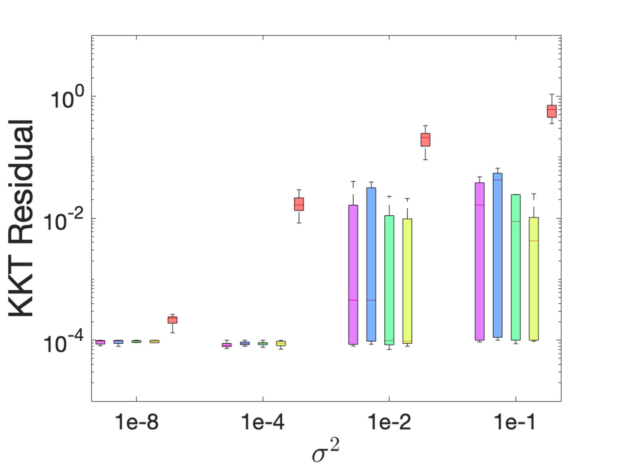
() $\beta_{k}=0.5$

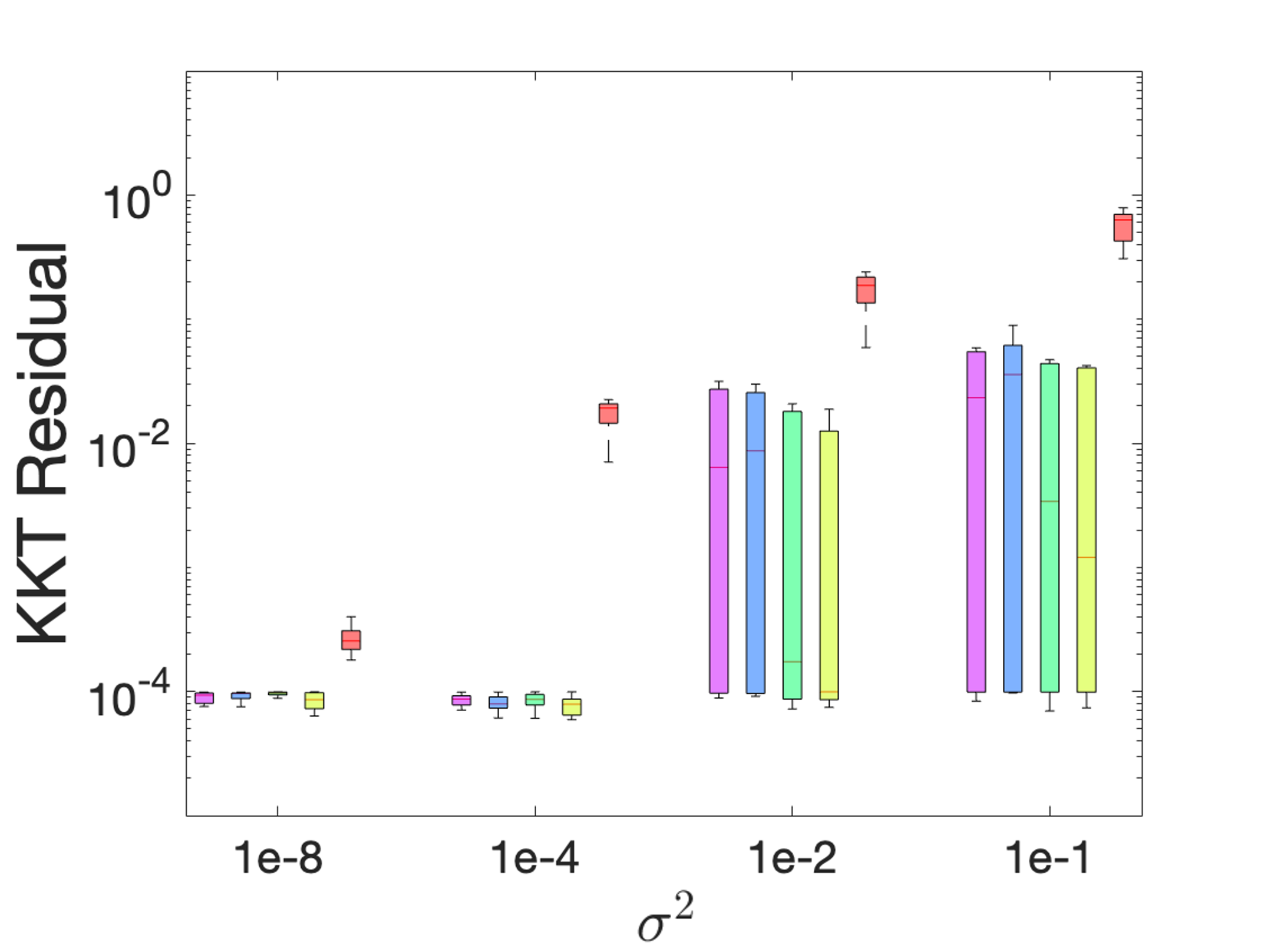
() $\beta_{k}=1.0$

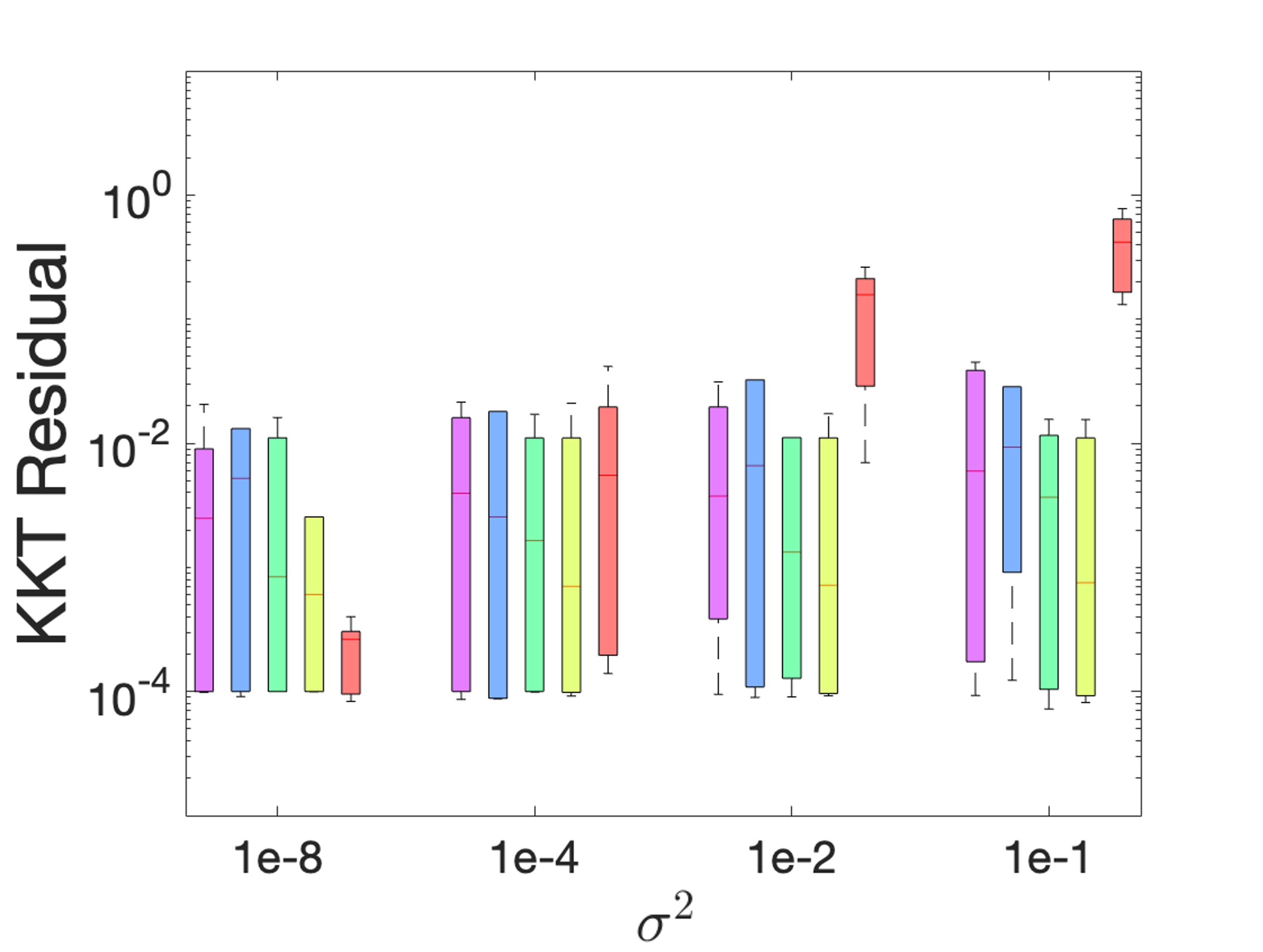
() $\beta_{k}=k^{-0.6}$

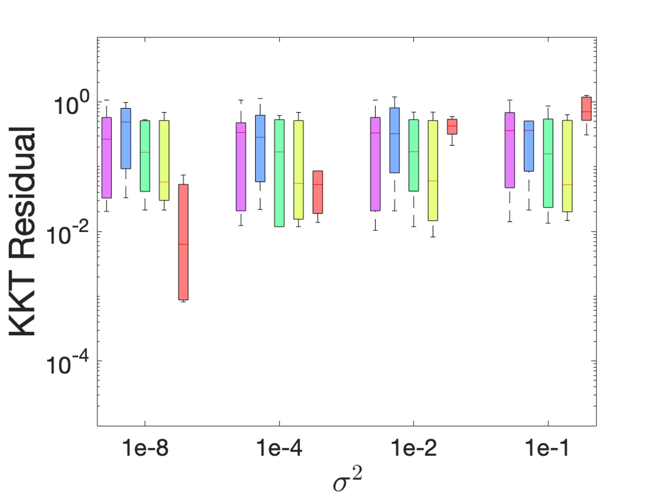
() $\beta_{k}=k^{-0.8}$

Figure 1: KKT residual boxplots for CUTEst problems. For each $\sigma^{2}$, there are five boxes. The first four boxes correspond to the proposed TR-StoSQP  method with four different choices of $B_{k}$, while the last box corresponds to the $\ell_{1}$-StoSQP method.

We then investigate the adaptivity of the radius selection scheme in (12). As explained in Remark 3.1, the radius $\Delta_{k}$ can be set larger or smaller than $\alpha_{k}=\mathcal{O}(\beta_{k})$, depending on the magnitude of the estimated KKT residual. In Table 1, we report the proportions of the three cases in (12): $\Delta_{k}<\alpha_{k}$, $\Delta_{k}=\alpha_{k}$, and $\Delta_{k}>\alpha_{k}$. We average the proportions over 5 runs of all 47 problems in each setup. From Table 1, we have the following three observations. (i) Case 2 has a near zero proportion for all setups. This phenomenon is due to the fact that $\eta_{1,k}-\eta_{2,k}=\mathcal{O}(\beta_{k})$. For constant $\beta_{k}$, this value is small, thus a few iterations are in Case 2. For decaying $\beta_{k}$, this value even converges to zero, thus almost no iterations are in Case 2. (ii) Case 3 is triggered quite frequently if $\beta_{k}$ decays rapidly. This phenomenon suggests that the adaptive scheme can generate aggressive steps even if we input a conservative radius-related sequence $\beta_{k}$. (iii) The proportion of Case 1 dominates the other two cases in the most of setups. This is reasonable since Case 1 is always triggered when the iterates are near a KKT point.

$\beta_{k}$	$B_{k}$	$\sigma^{2}=10^{-8}$			$\sigma^{2}=10^{-4}$			$\sigma^{2}=10^{-2}$			$\sigma^{2}=10^{-1}$
		Case 1	Case 2	Case 3	Case 1	Case 2	Case 3	Case 1	Case 2	Case 3	Case 1	Case 2	Case 3
0.5	Id	90.3	0.1	9.6	91.3	0.2	8.5	95.0	0.1	4.9	54.7	0.9	44.4
	SR1	93.8	0.1	6.1	92.7	0.1	7.2	94.6	0.1	5.7	56.2	1.1	42.7
	EstH	92.2	0.1	7.7	94.8	0.1	5.1	84.8	0.2	15.0	71.1	0.5	28.4
	AveH	92.5	0.1	7.4	94.1	0.1	5.8	88.2	0.2	11.6	64.2	0.4	35.4
1.0	Id	92.0	0.1	7.9	93.7	0.1	6.2	95.4	0.2	4.4	57.1	1.2	41.7
	SR1	94.0	0.2	5.8	96.1	0.1	3.8	97.7	0.2	2.1	64.2	1.2	34.6
	EstH	92.4	0.1	7.5	93.8	0.1	6.1	87.5	0.4	12.1	72.8	0.5	26.7
	AveH	92.4	0.2	7.4	93.9	0.3	5.8	85.5	0.3	14.2	67.1	0.6	32.3
$k^{-0.6}$	Id	97.2	0.0	2.8	96.8	0.0	3.2	93.4	0.0	6.6	51.8	0.0	48.2
	SR1	98.3	0.0	1.7	97.1	0.0	2.9	93.2	0.0	6.8	51.5	0.0	48.5
	EstH	97.9	0.0	2.1	95.8	0.0	4.2	86.6	0.0	13.4	69.1	0.0	30.9
	AveH	97.4	0.0	2.6	96.1	0.0	3.9	86.8	0.0	13.2	65.5	0.0	34.8
$k^{-0.8}$	Id	70.6	0.0	29.4	68.1	0.0	31.9	66.4	0.0	33.6	45.8	0.0	54.2
	SR1	56.1	0.0	43.9	65.7	0.0	34.3	66.6	0.0	33.4	39.9	0.0	60.1
	EstH	67.5	0.0	32.5	65.2	0.0	34.8	62.0	0.0	38.0	54.7	0.0	45.3
	AveH	67.9	0.0	32.1	66.7	0.0	33.3	65.9	0.0	34.1	51.4	0.0	48.6

Table 1: Proportions of the three cases in (12) (%). We highlight the proportion of Case 3 if the value is higher than 25%.

In Remark 3.4, we provide two alternative relaxation techniques to compute the trial step. Figure 2 reports the KKT residuals for these methods. We use Adap1 to denote TR-StoSQP with our adaptive relaxation technique; Adap2 to denote TR-StoSQP with the technique in Remark 3.4(i), where the radius of the tangential step is controlled by $\widetilde{\Delta}_{k}\coloneqq\sqrt{\Delta_{k}^{2}-\|\bm{w}_{k}\|^{2}}$; and NonAdap to denote TR-StoSQP with the technique in Remark 3.4(ii), where the prespecified parameter is set as $\theta=0.8$. The remaining algorithm setups follow from TR-StoSQP and $B_{k}=I$. We observe that the three techniques have comparable performance for most combinations of $\beta_{k}$ and $\sigma^{2}$, while Adap1 is slightly better than the other two techniques in some cases. The results suggest that our adaptive relaxation technique, as well as its variant in Remark 3.4(i), is at least as good as the conventional technique (the nonadaptive technique in Remark 3.4(ii)) in practice, but it requires no effort in tuning parameters.

() $\beta_{k}=0.5$

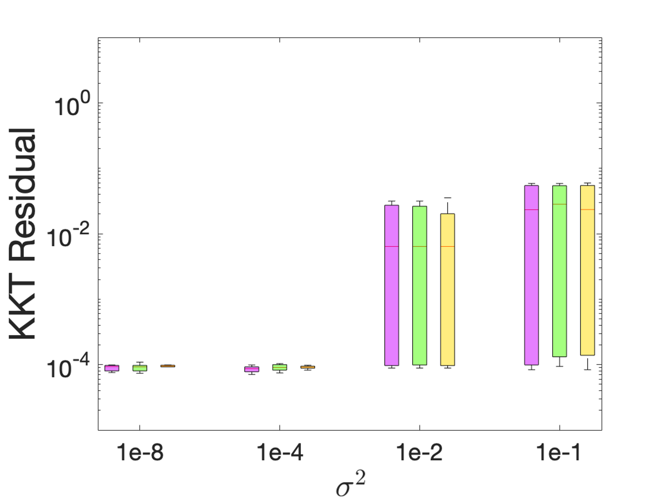
() $\beta_{k}=1.0$

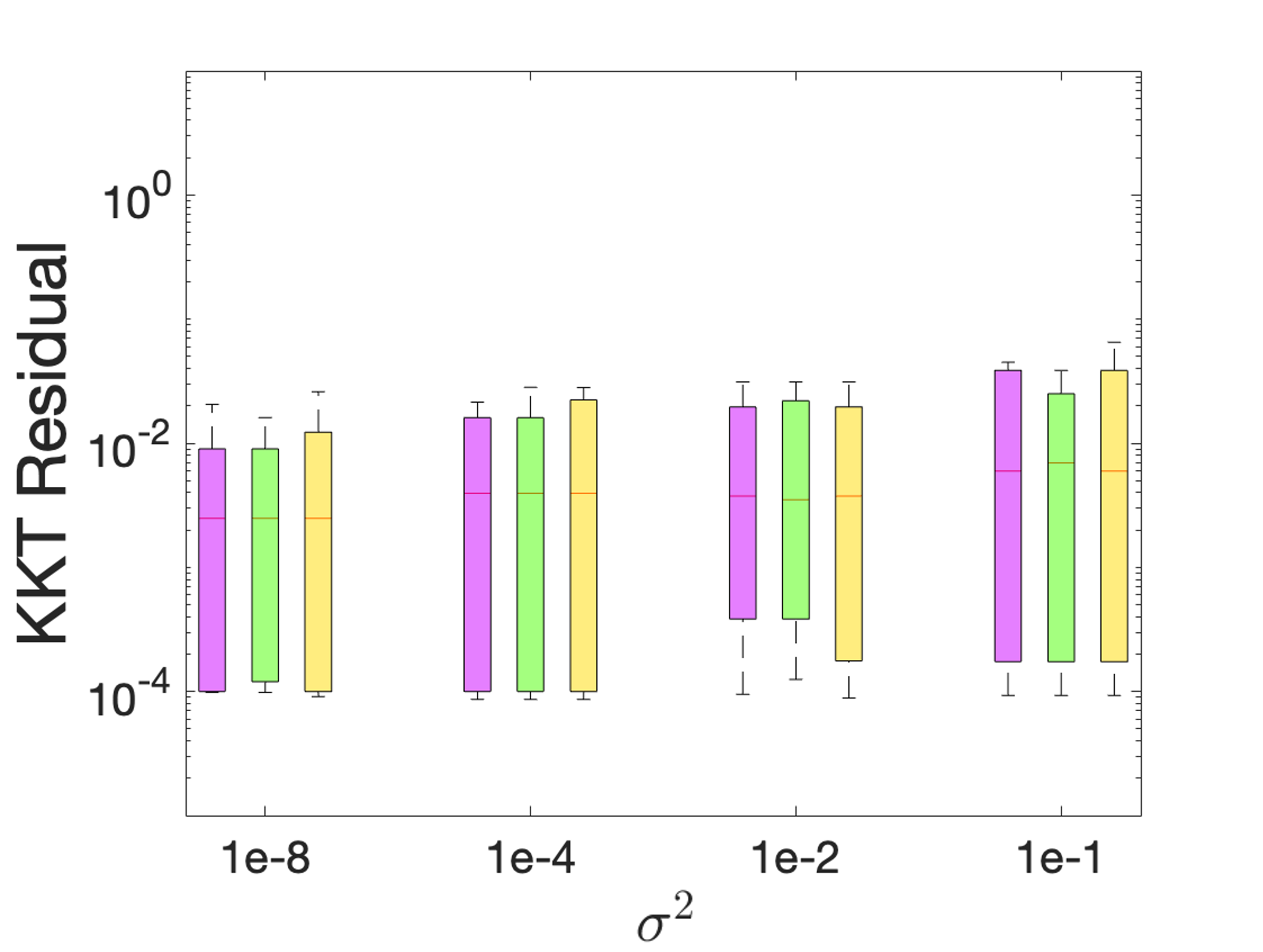
() $\beta_{k}=k^{-0.6}$

() $\beta_{k}=k^{-0.8}$

Figure 2: KKT residual boxplots for CUTEst problems with different relaxation techniques. The Hessian approximation $B_{k}$ is set as identity matrix. For each $\sigma^{2}$, there are three boxes. The first box corresponds to the proposed adaptive relaxation technique. The second box corresponds to the adaptive technique in Remark 3.4 (i). The last box corresponds to the nonadaptive technique in Remark 3.4 (ii).

5.3 Constrained logistic regression

We consider equality-constrained logistic regression of the form

$$\min_{{\bm{x}}\in\mathbb{R}^{d}}\;f({\bm{x}})=\frac{1}{N}\sum_{i=1}^{N}\log\left\{1+\exp\left(-y_{i}\cdot\langle{\bm{z}}_{i},{\bm{x}}\rangle\right)\right\}\quad\text{ s.t. }A{\bm{x}}=\bm{b},$$

where ${\bm{z}}_{i}\in\mathbb{R}^{d}$ is the sample point, $y_{i}\in\{-1,1\}$ is the label, and $A\in\mathbb{R}^{m\times d}$ and ${\bm{b}}\in\mathbb{R}^{m}$ form the deterministic constraints. We implement 8 datasets from LIBSVM (Chang and Lin, 2011): austrilian, breast-cancer, diabetes, heart, ionosphere, sonar, splice, and svmguide3. For each dataset, we set $m=5$ and generate random $A$ and $\bm{b}$ by drawing each element from a standard normal distribution. We ensure that $A$ has full row rank in all problems. For both algorithms and all problems, the initial iterate is set to be all one vector of appropriate dimension. In each iteration, we select one sample at random to estimate the objective gradient (and Hessian if EstH or AveH is used). A budget of 20 epochs—the number of passes over the dataset—is used for both algorithms and all problems. We stop the iteration if $\|\nabla\mathcal{L}_{k}\|\leq 10^{-4}$ or the epoch budget is consumed.

We report the average of the KKT residuals over 5 runs in Figure 3. From the figure, we observe that TR-StoSQP  with all four choices of $B_{k}$ consistently outperforms $\ell_{1}$-StoSQP when $\beta_{k}=0.5$, $1.0$, and $k^{-0.6}$. When $\beta_{k}=k^{-0.8}$, TR-StoSQP  enjoys a better performance by using the estimated Hessian or averaged Hessian. This experiment further illustrates the promising performance of our method.

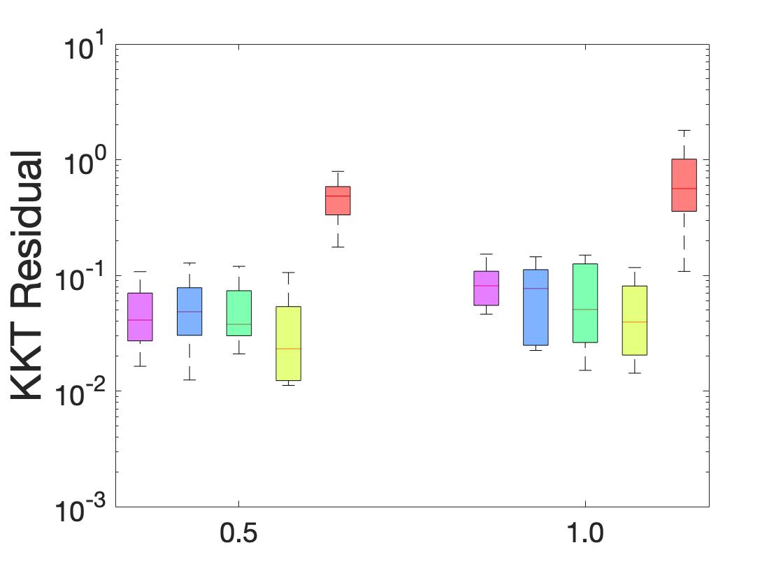
() Constant $\beta_{k}$

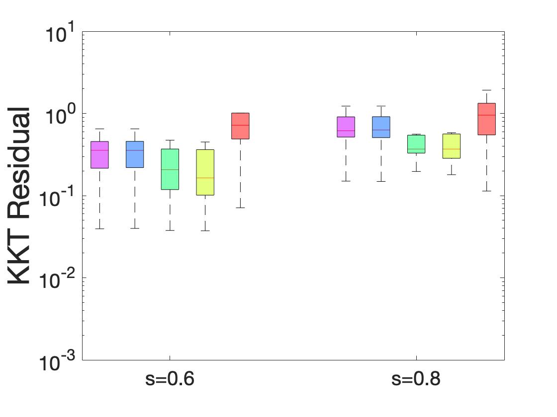
() Decaying $\beta_{k}=k^{-s}$

Figure 3: KKT residual boxplots for constrained logistic regression problems. For each setup of $\beta_{k}$, there are five boxes. The first four boxes correspond to the proposed TR-StoSQP  method with four different choices of $B_{k}$, while the last box corresponds to the $\ell_{1}$-StoSQP method.

6 Conclusion

We designed a trust-region stochastic SQP (TR-StoSQP) algorithm to solve nonlinear optimization problems with stochastic objective and deterministic equality constraints. We developed an adaptive relaxation technique to address the infeasibility issue that arises when trust-region methods are applied to constrained problems. With a stabilized merit parameter, TR-StoSQP converges in two regimes. (i) When $\beta_{k}=\beta$, $\forall k\geq 0$, the expectation of weighted averaged KKT residuals converges to a neighborhood around zero. (ii) When $\beta_{k}$ satisfies $\sum\beta_{k}=\infty$ and $\sum\beta_{k}^{2}<\infty$, the KKT residuals converge to zero almost surely. We also showed that the merit parameter is ensured to stabilize, provided the gradient estimates are bounded. Our numerical experiments on a subset of problems of the CUTEst set and constrained logistic regression problems showed promising performance of the proposed method.

There are still several interesting future directions. First, it is of interest to design trust-region StoSQP algorithms when the Jacobians of constraints are rank-deficient. Second, how to establish global convergence without the assumption of bounded noise remains an open question. Removing that assumption may require a deeper understanding of the merit function and randomness in estimation. Finally, it is of interest to devise a method that uses second-order information efficiently. To fully exploit second-order derivatives, the method should move the trial steps along the negative curvature appropriately.

Acknowledgments

We would like to acknowledge the DOE, NSF, and ONR as well as the J. P. Morgan Chase Faculty Research Award for providing partial support of this work.

Appendix A Additional Analysis of the Behavior of the Merit Parameter

In the appendix, we further investigate the stability behavior of the merit parameter when using the alternative two approaches in Remark 3.4 to decompose the radius. As mentioned, for both approaches, the global convergence analysis directly follows from Section 4.2.

We first show that for the method in Remark 3.4(i), the merit parameter will stabilize under Assumption 4.12.

Lemma A.1.

Suppose Assumptions 4.1 and 4.12 hold and the relaxation technique in Remark 3.4(i) is employed. Then, there exist a (potentially random) ${\bar{K}}<\infty$ and a deterministic constant $\widehat{\mu}$, such that ${\bar{\mu}}_{k}={\bar{\mu}}_{{\bar{K}}}\leq{\widehat{\mu}}$, $\forall k>{\bar{K}}$.

Proof.

Similar to Lemma 4.13, we only show that there exists a deterministic threshold $\widetilde{\mu}>0$ independent of $k$ such that (16) is satisfied as long as ${\bar{\mu}}_{k}\geq\widetilde{\mu}$. Using the same derivation as Lemma 4.13, we have

$$\text{Pred}_{k} \leq-\|\bar{\nabla}_{{\bm{x}}}{\mathcal{L}}_{k}\|\widetilde{\Delta}_{k}+{\bar{\gamma}}_{k}\|B_{k}\|\|{\bm{v}}_{k}\|\widetilde{\Delta}_{k}+\frac{1}{2}\|B_{k}\|\widetilde{\Delta}_{k}^{2}+{\bar{\gamma}}_{k}(M_{1}+\kappa_{\nabla f})\|{\bm{v}}_{k}\|$$

$$\quad+\frac{1}{2}{\bar{\gamma}}_{k}\|B_{k}\|\|{\bm{v}}_{k}\|^{2}-{\bar{\mu}}_{k}{\bar{\gamma}}_{k}\|c_{k}\|$$

$$\leq-\|\bar{\nabla}_{{\bm{x}}}{\mathcal{L}}_{k}\|\Delta_{k}+{\bar{\gamma}}_{k}\|{\bm{v}}_{k}\|\|\bar{\nabla}_{{\bm{x}}}{\mathcal{L}}_{k}\|+{\bar{\gamma}}_{k}\|B_{k}\|\|{\bm{v}}_{k}\|\widetilde{\Delta}_{k}+\frac{1}{2}\|B_{k}\|\widetilde{\Delta}_{k}^{2}$$

$$\quad+{\bar{\gamma}}_{k}(M_{1}+\kappa_{\nabla f})\|{\bm{v}}_{k}\|+\frac{1}{2}{\bar{\gamma}}_{k}\|B_{k}\|\|{\bm{v}}_{k}\|^{2}-{\bar{\mu}}_{k}{\bar{\gamma}}_{k}\|c_{k}\|\quad(\text{since }\widetilde{\Delta}_{k}\geq\Delta_{k}-{\bar{\gamma}}_{k}\|{\bm{v}}_{k}\|)$$

$$=-\|\bar{\nabla}_{{\bm{x}}}{\mathcal{L}}_{k}\|\Delta_{k}-\|c_{k}\|\Delta_{k}+\|c_{k}\|\Delta_{k}+{\bar{\gamma}}_{k}\|{\bm{v}}_{k}\|\|\bar{\nabla}_{{\bm{x}}}{\mathcal{L}}_{k}\|+{\bar{\gamma}}_{k}\|B_{k}\|\|{\bm{v}}_{k}\|\widetilde{\Delta}_{k}$$

$$\quad+\frac{1}{2}\|B_{k}\|\widetilde{\Delta}_{k}^{2}+{\bar{\gamma}}_{k}(M_{1}+\kappa_{\nabla f})\|{\bm{v}}_{k}\|+\frac{1}{2}{\bar{\gamma}}_{k}\|B_{k}\|\|{\bm{v}}_{k}\|^{2}-{\bar{\mu}}_{k}{\bar{\gamma}}_{k}\|c_{k}\|$$

$$\leq-\|\bar{\nabla}{\mathcal{L}}_{k}\|\Delta_{k}+\frac{1}{2}\|B_{k}\|\Delta_{k}^{2}+\|c_{k}\|\Delta_{k}+{\bar{\gamma}}_{k}\|{\bm{v}}_{k}\|\|\bar{\nabla}_{{\bm{x}}}{\mathcal{L}}_{k}\|+{\bar{\gamma}}_{k}\|B_{k}\|\|{\bm{v}}_{k}\|\Delta_{k}$$

$$\quad+{\bar{\gamma}}_{k}(M_{1}+\kappa_{\nabla f})\|{\bm{v}}_{k}\|+\frac{1}{2}{\bar{\gamma}}_{k}\|B_{k}\|\|{\bm{v}}_{k}\|^{2}-{\bar{\mu}}_{k}{\bar{\gamma}}_{k}\|c_{k}\|,$$

since $\|\bar{\nabla}_{{\bm{x}}}{\mathcal{L}}_{k}\|+\|c_{k}\|\geq\|\bar{\nabla}{\mathcal{L}}_{k}\|$ and $\widetilde{\Delta}_{k}\leq\Delta_{k}$. Thus, (16) holds as long as

$${\bar{\mu}}_{k}{\bar{\gamma}}_{k}\|c_{k}\|\geq\|c_{k}\|\Delta_{k}+{\bar{\gamma}}_{k}\|{\bm{v}}_{k}\|\|\bar{\nabla}_{{\bm{x}}}{\mathcal{L}}_{k}\|+{\bar{\gamma}}_{k}\|B_{k}\|\|{\bm{v}}_{k}\|\Delta_{k}+{\bar{\gamma}}_{k}(M_{1}+\kappa_{\nabla f})\|{\bm{v}}_{k}\|+\frac{{\bar{\gamma}}_{k}}{2}\|B_{k}\|\|{\bm{v}}_{k}\|^{2}.$$

Since $\|{\bm{v}}_{k}\|\leq\|c_{k}\|/\sqrt{\kappa_{1,G}}$, $\|\bar{\nabla}_{{\bm{x}}}{\mathcal{L}}_{k}\|\leq\|\nabla_{{\bm{x}}}{\mathcal{L}}_{k}\|+\|\nabla f_{k}-{\bar{g}}_{k}\|\leq\kappa_{\nabla f}+M_{1}$ and $\Delta_{k}\leq\Delta_{\max}$, it is sufficient to show

$${\bar{\mu}}_{k}{\bar{\gamma}}_{k}\|c_{k}\|\geq\|c_{k}\|\Delta_{k}+{\bar{\gamma}}_{k}\|c_{k}\|\left(\frac{\kappa_{B}\Delta_{\max}+2(M_{1}+\kappa_{\nabla f})}{\sqrt{\kappa_{1,G}}}+\frac{\kappa_{B}\kappa_{c}}{2\kappa_{1,G}}\right).$$

Equivalently,

$${\bar{\mu}}_{k}\geq\frac{\Delta_{k}}{{\bar{\gamma}}_{k}}+\left(\frac{\kappa_{B}\Delta_{\max}+2(M_{1}+\kappa_{\nabla f})}{\sqrt{\kappa_{1,G}}}+\frac{\kappa_{B}\kappa_{c}}{2\kappa_{1,G}}\right).$$

Here, we only consider $\|c_{k}\|\neq 0$ since the result trivially holds when $\|c_{k}\|=0$. From (12), we find that

$$\frac{\Delta_{k}}{{\bar{\gamma}}_{k}}\leq\frac{\eta_{1,k}\alpha_{k}\|\bar{\nabla}{\mathcal{L}}_{k}\|}{{\bar{\gamma}}_{k}}.$$

By (26), ${\bar{\gamma}}_{k}\geq\frac{1}{2}\zeta\phi_{k}\alpha_{k}=\frac{1}{2}\zeta\min\{\|B_{k}\|/\|G_{k}\|,1\}\alpha_{k}$. Noting that $\min\{\|B_{k}\|/\|G_{k}\|,1\}\geq\min\{1/(\kappa_{B}\sqrt{\kappa_{2,G}}),1\}$ and $\|\bar{\nabla}{\mathcal{L}}_{k}\|\leq\kappa_{c}+M_{1}+\kappa_{\nabla f}$, we obtain

$$\frac{\Delta_{k}}{{\bar{\gamma}}_{k}}\leq\frac{2\eta_{\max}}{\zeta}(\kappa_{c}+\kappa_{\nabla f}+M_{1})\cdot\max\{\kappa_{B}\sqrt{\kappa_{2,G}},1\}.$$

Therefore, (16) holds as long as

$${\bar{\mu}}_{k}\geq\widetilde{\mu}\coloneqq\frac{2\eta_{\max}}{\zeta}(\kappa_{c}+\kappa_{\nabla f}+M_{1})\cdot\max\{\kappa_{B}\sqrt{\kappa_{2,G}},1\}+\left(\frac{\kappa_{B}\Delta_{\max}+2(M_{1}+\kappa_{\nabla f})}{\sqrt{\kappa_{1,G}}}+\frac{\kappa_{B}\kappa_{c}}{2\kappa_{1,G}}\right).$$

Since ${\bar{\mu}}_{k}$ is increased by at least a factor of $\rho$ for each update, we define $\widehat{\mu}\coloneqq\rho\widetilde{\mu}$ and complete the proof. ∎

We then show that for the method in Remark 3.4(ii), the merit parameter will stabilize just under Assumption 4.12(i). However, a tuning parameter $\theta\in(0,1)$ is involved to control the length of the normal step.

Lemma A.2.

Suppose Assumptions 4.1 and 4.12(i) hold and the relaxation technique in Remark 3.4(ii) is employed. Then, there exist a (potentially random) ${\bar{K}}<\infty$ and a deterministic constant $\widehat{\mu}$, such that ${\bar{\mu}}_{k}={\bar{\mu}}_{{\bar{K}}}\leq{\widehat{\mu}}$, $\forall k>{\bar{K}}$.

Proof.

Similar to Lemma 4.13, we only show that there exists a deterministic threshold $\widetilde{\mu}>0$ independent of $k$ such that (16) is satisfied as long as ${\bar{\mu}}_{k}\geq\widetilde{\mu}$. Using the same derivation as Lemma A.1, we only need to show

$${\bar{\mu}}_{k}\geq\frac{\Delta_{k}}{{\bar{\gamma}}_{k}}+\left(\frac{\kappa_{B}\Delta_{\max}+2(M_{1}+\kappa_{\nabla f})}{\sqrt{\kappa_{1,G}}}+\frac{\kappa_{B}\kappa_{c}}{2\kappa_{1,G}}\right)$$

holds for ${\bar{\mu}}_{k}$ larger than a deterministic threshold for $\|c_{k}\|\neq 0$. Since for $\forall k\geq 0$,

$$\frac{\Delta_{k}}{{\bar{\gamma}}_{k}}\leq\frac{\eta_{1,k}\alpha_{k}\|\bar{\nabla}{\mathcal{L}}_{k}\|}{{\bar{\gamma}}_{k}}.$$

By the projection technique of choosing ${\bar{\gamma}}_{k}$ and the fact that $\eta_{2,k}\geq\eta_{1,k}/2$, we have

$$\frac{\breve{\Delta}_{k}}{\|{\bm{v}}_{k}\|}=\frac{\theta\Delta_{k}}{\|{\bm{v}}_{k}\|}\stackrel{{\scriptstyle\eqref{Ful_GenerateRadius}}}{{\geq}}\frac{\theta\eta_{2,k}\alpha_{k}\|{\bar{\nabla}}\mathcal{L}_{k}\|}{\|{\bm{v}}_{k}\|}\geq\frac{\theta\eta_{1,k}\alpha_{k}\|c_{k}\|}{2\|{\bm{v}}_{k}\|}\stackrel{{\scriptstyle\eqref{def:eta2k}}}{{=}}\frac{\theta\zeta\alpha_{k}}{2}.$$

Further, since $\theta\zeta\alpha_{k}/2\leq 1$, we know $\theta\zeta\alpha_{k}/2\leq{\bar{\gamma}}_{k}^{\text{trial}}$, implying ${\bar{\gamma}}_{k}\geq\theta\zeta\alpha_{k}/2$. Thus,

$$\frac{\Delta_{k}}{{\bar{\gamma}}_{k}}\leq\frac{2\eta_{\max}}{\zeta\theta}(\kappa_{c}+\kappa_{\nabla f}+M_{1}).$$

Therefore, (16) holds as long as

$${\bar{\mu}}_{k}\geq\widetilde{\mu}\coloneqq\frac{2\eta_{\max}}{\zeta\theta}(\kappa_{c}+\kappa_{\nabla f}+M_{1})+\left(\frac{\kappa_{B}\Delta_{\max}+2(M_{1}+\kappa_{\nabla f})}{\sqrt{\kappa_{1,G}}}+\frac{\kappa_{B}\kappa_{c}}{2\kappa_{1,G}}\right).$$

Since ${\bar{\mu}}_{k}$ is increased by at least a factor of $\rho$ for each update, we define $\widehat{\mu}\coloneqq\rho\widetilde{\mu}$ and complete the proof. ∎

References

- Berahas et al. (2021a) A. S. Berahas, F. E. Curtis, M. J. O’Neill, and D. P. Robinson. A stochastic sequential quadratic optimization algorithm for nonlinear equality constrained optimization with rank-deficient jacobians. arXiv preprint arXiv:2106.13015, 2021a.
- Berahas et al. (2021b) A. S. Berahas, F. E. Curtis, D. Robinson, and B. Zhou. Sequential quadratic optimization for nonlinear equality constrained stochastic optimization. SIAM Journal on Optimization, 31(2):1352–1379, 2021b.
- Berahas et al. (2022a) A. S. Berahas, R. Bollapragada, and B. Zhou. An adaptive sampling sequential quadratic programming method for equality constrained stochastic optimization. arXiv preprint arXiv:2206.00712, 2022a.
- Berahas et al. (2022b) A. S. Berahas, J. Shi, Z. Yi, and B. Zhou. Accelerating stochastic sequential quadratic programming for equality constrained optimization using predictive variance reduction. arXiv preprint arXiv:2204.04161, 2022b.
- Bertsekas (1998) D. Bertsekas. Network optimization: continuous and discrete models, volume 8. Athena Scientific, 1998.
- Bertsekas (1982) D. P. Bertsekas. Constrained Optimization and Lagrange Multiplier Methods. Elsevier, 1982.
- Birge (1997) J. R. Birge. State-of-the-art-survey—stochastic programming: Computation and applications. INFORMS Journal on Computing, 9(2):111–133, 1997.
- Boggs and Tolle (1995) P. T. Boggs and J. W. Tolle. Sequential quadratic programming. Acta Numerica, 4:1–51, 1995.
- Bottou et al. (2018) L. Bottou, F. E. Curtis, and J. Nocedal. Optimization methods for large-scale machine learning. SIAM Review, 60(2):223–311, 2018.
- Byrd et al. (1987) R. H. Byrd, R. B. Schnabel, and G. A. Shultz. A trust region algorithm for nonlinearly constrained optimization. SIAM Journal on Numerical Analysis, 24(5):1152–1170, 1987.
- Celis et al. (1984) M. R. Celis, J. Dennis Jr, and R. A. Tapia. A trust region strategy for equality constrained optimization. Technical report, 1984.
- Chang and Lin (2011) C.-C. Chang and C.-J. Lin. LIBSVM: A library for support vector machines. ACM Transactions on Intelligent Systems and Technology, 2(3):1–27, 2011.
- Chen et al. (2018) C. Chen, F. Tung, N. Vedula, and G. Mori. Constraint-aware deep neural network compression. In Computer Vision – ECCV 2018, pages 409–424. Springer International Publishing, 2018.
- Chen et al. (2017) R. Chen, M. Menickelly, and K. Scheinberg. Stochastic optimization using a trust-region method and random models. Mathematical Programming, 169(2):447–487, 2017.
- Chen et al. (2020) Y.-L. Chen, S. Na, and M. Kolar. Convergence analysis of accelerated stochastic gradient descent under the growth condition. arXiv preprint arXiv:2006.06782, 2020.
- Curtis and Robinson (2018) F. E. Curtis and D. P. Robinson. Exploiting negative curvature in deterministic and stochastic optimization. Mathematical Programming, 176(1-2):69–94, 2018.
- Curtis and Shi (2020) F. E. Curtis and R. Shi. A fully stochastic second-order trust region method. Optimization Methods and Software, 37(3):844–877, 2020.
- Curtis et al. (2019) F. E. Curtis, K. Scheinberg, and R. Shi. A stochastic trust region algorithm based on careful step normalization. INFORMS Journal on Optimization, 1(3):200–220, 2019.
- Curtis et al. (2021a) F. E. Curtis, M. J. O’Neill, and D. P. Robinson. Worst-case complexity of an sqp method for nonlinear equality constrained stochastic optimization. arXiv preprint arXiv:2112.14799, 2021a.
- Curtis et al. (2021b) F. E. Curtis, D. P. Robinson, and B. Zhou. Inexact sequential quadratic optimization for minimizing a stochastic objective function subject to deterministic nonlinear equality constraints. arXiv preprint arXiv:2107.03512, 2021b.
- Dupacova and Wets (1988) J. Dupacova and R. Wets. Asymptotic behavior of statistical estimators and of optimal solutions of stochastic optimization problems. The Annals of Statistics, 16(4):1517–1549, 1988.
- El-Alem (1991) M. El-Alem. A global convergence theory for the celis–dennis–tapia trust-region algorithm for constrained optimization. SIAM Journal on Numerical Analysis, 28(1):266–290, 1991.
- Gould et al. (2014) N. I. M. Gould, D. Orban, and P. L. Toint. CUTEst: a constrained and unconstrained testing environment with safe threads for mathematical optimization. Computational Optimization and Applications, 60(3):545–557, 2014.
- Johnson and Zhang (2013) R. Johnson and T. Zhang. Accelerating stochastic gradient descent using predictive variance reduction. Advances in neural information processing systems, 26, 2013.
- Na and Mahoney (2022) S. Na and M. W. Mahoney. Asymptotic convergence rate and statistical inference for stochastic sequential quadratic programming. arXiv preprint arXiv:2205.13687, 2022.
- Na et al. (2021) S. Na, M. Anitescu, and M. Kolar. Inequality constrained stochastic nonlinear optimization via active-set sequential quadratic programming. arXiv preprint arXiv:2109.11502, 2021.
- Na et al. (2022a) S. Na, M. Anitescu, and M. Kolar. An adaptive stochastic sequential quadratic programming with differentiable exact augmented lagrangians. Mathematical Programming, 2022a.
- Na et al. (2022b) S. Na, M. Dereziński, and M. W. Mahoney. Hessian averaging in stochastic Newton methods achieves superlinear convergence. arXiv preprint arXiv:2204.09266, 2022b.
- Nocedal and Wright (2006) J. Nocedal and S. Wright. Numerical Optimization. Springer New York, 2006.
- Omojokun (1989) E. O. Omojokun. Trust region algorithms for optimization with nonlinear equality and inequality constraints. PhD thesis, University of Colorado, Boulder, CO, 1989.
- Powell and Yuan (1990) M. J. D. Powell and Y. Yuan. A trust region algorithm for equality constrained optimization. Mathematical Programming, 49(1-3):189–211, 1990.
- Rees et al. (2010) T. Rees, H. S. Dollar, and A. J. Wathen. Optimal solvers for PDE-constrained optimization. SIAM Journal on Scientific Computing, 32(1):271–298, 2010.
- Robbins and Siegmund (1971) H. Robbins and D. Siegmund. A convergence theorem for non negative almost supermartingales and some applications. In Optimizing Methods in Statistics, pages 233–257. Elsevier, 1971.
- Stich (2019) S. U. Stich. Unified optimal analysis of the (stochastic) gradient method. arXiv preprint arXiv:1907.04232, 2019.
- Sun and Nocedal (2023) S. Sun and J. Nocedal. A trust region method for noisy unconstrained optimization. Mathematical Programming, pages 1–28, 2023.
- Vardi (1985) A. Vardi. A trust region algorithm for equality constrained minimization: Convergence properties and implementation. SIAM Journal on Numerical Analysis, 22(3):575–591, 1985.
- Vaswani et al. (2019) S. Vaswani, F. Bach, and M. Schmidt. Fast and faster convergence of sgd for over-parameterized models and an accelerated perceptron. In The 22nd international conference on artificial intelligence and statistics, pages 1195–1204. PMLR, 2019.
- Wächter and Biegler (2005) A. Wächter and L. T. Biegler. On the implementation of an interior-point filter line-search algorithm for large-scale nonlinear programming. Mathematical Programming, 106(1):25–57, 2005.
- Yuan (1990) Y. Yuan. On a subproblem of trust region algorithms for constrained optimization. Mathematical Programming, 47(1-3):53–63, 1990.
- Yuan (1991) Y. Yuan. A dual algorithm for minimizing a quadratic function with two quadratic constraints. Journal of Computational mathematics, pages 348–359, 1991.
- Zhang (1992) Y. Zhang. Computing a celis-dennis-tapia trust-region step for equality constrained optimization. Mathematical Programming, 55(1-3):109–124, 1992.