Universal quantum computer based on Carbon Nanotube Rotators

Abstract

We propose a universal quantum computer based on a chain of carbon nanotube rotators where one metallic plate is attached to each rotator. The dynamical variable is the rotational angle $\phi$. The attached plate connected to ground electrostatically interacts with two fixed plates. Two angle positions $\phi=0,\pi$ are made stable by applying a voltage difference between the attached plate and the two fixed plates. We assign $\phi=0$ and $\pi$ to the qubit states $|0\rangle$ and $|1\rangle$. Then, considering a chain of rotators, we construct the arbitrary phase-shift gate, the NOT gate and the Ising gate, which constitute a set of universal quantum gates. They are executed by controlling the voltage between various plates.

I Introduction

The Moor law is a fundamental roadmap of integrated circuits, which dictates that the number of elements increases exponentially as a function of year. It also means that the size of an element must become exponentially small. However, there is an intrinsic limit of an element, which is the size of atoms of the order of 1nm. It gives a limit to the Moor law. The quantum computer is expected to be a solution to overcome it[1, 2, 3]. Quantum computers are based on qubits, where the superposition of the quantum states $|0\rangle$ and $|1\rangle$ is used. Various methods have been proposed such as superconductors[4], photonic systems[5], ion trap[6], nuclear magnetic resonance[7, 8], quantum dots[9], skyrmions[10, 11] and merons[12]. Nanomechanical systems are also applicable to quantum computers[13, 14, 15, 16].

Quantum algorithm is decomposed into a sequential application of quantum gates. The Solovay-Kitaev theorem assures that only three quantum gates, the $\pi/4$ phase-shift gate, the Hadamard gates and the CNOT gate, are enough for universal quantum computations[17, 18, 19]. Alternatively, the arbitrary phase-shift gate, the NOT gate and the Ising gate constitute a set of universal quantum gates as well.

Nano-electromechanical systems (NEMS)[20, 21] have various industrial applications. A nanorotator based on a carbon nanotube has been experimentally realized[22, 23, 24, 25]. Especially, a double-wall nanotube structure acts as a nanomotor[26, 23, 27, 28, 24, 29, 25, 30]. A carbon nanotube can be metallic depending on the chirality of a nanotube[31]. In addition, it is possible to attach a metallic plate to a nanotube[22, 27]. Quantum effects are experimentally observed in NEMS[32, 33, 34].

In this paper, we propose a universal quantum computer by constructing a set of universal quantum gates. We prepare a rotator based on a double-wall nanotube as illustrated in Fig.1(a). We attach one metallic plate to the inner nanotube. It is possible to materialize such a nanorotator by using the present techniques[22, 27]. Then, we align these rotators along a line with equal spacing, which is the main configuration of our proposal. We explicitly design the arbitrary phase-shift gate, the NOT gate and the Ising gate. They are controlled by the voltage between two plates.

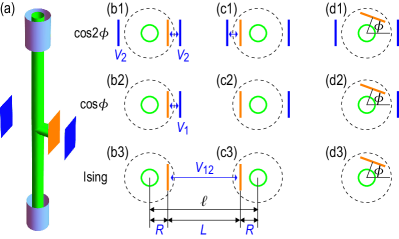
Figure 1: (a) Illustration of a nanotube rotator suspended by the double-wall nanotube structures at the top and the bottom. One metallic plate (in orange) is attached to the nanotube. Two metallic plates (in blue) are fixed to the outer system. We connect the inner plate to ground. When we give a voltage to the two outer plates, the $\cos 2\phi$ potential is induced. When we give a voltage to one of the two outer plates, the $\cos\phi$ potential is induced. On the other hand, when we give a voltage between the two plates attached to two nanotubes, the Ising interaction is induced. (b) The configuration of a rotator with $\phi=0$, representing the qubit state $\left|0\right\rangle$. (c) The configuration of a rotator with $\phi=\pi$, representing the qubit state $\left|1\right\rangle$. (d) The configuration of a rotator with a generic angle $\phi$. Dotted circles denote the rotator parts.

II Model

II.1 Carbon nanotube rotator

We consider a rotator whose dynamical variable is the rotational angle $\phi$ with the potential energy given by[27]

$$W_{2}(\phi)=-A\cos 2\phi.$$ (1)

There are two stable angles $\phi=0$ and $\pi$, which we regard to form one-qubit states {$|0\rangle,|1\rangle$}. In addition, we introduce a potential term given by[27]

$$W_{1}(\phi)=-B\cos\phi,$$ (2)

which resolves the degeneracy between the states $|0\rangle$ and $|1\rangle$.

The Schrödinger equation for one rotator reads

$$i\hbar\frac{d}{dt}\psi\left(t\right)=H\psi\left(t\right),$$ (3)

with the Hamiltonian given by

$$H=-\frac{\hbar^{2}}{2\mu r^{2}}\frac{\partial}{\partial\phi^{2}}-A\cos 2\phi-B\cos\phi,$$ (4)

where $\mu$ is the inertia of the rotator and $r$ is the radius of the rotator. The eigenequation reads

$$H\psi=E\psi.$$ (5)

The Hamiltonian (4) may be materialized by a rotator, which is made of a nanotube (in green) supported by the double-wall nanotube structures at the top and the bottom, as illustrated in Fig.1(a). We attach one metal plate (in orange) to the nanotube, which we call the inner plate. Then, we introduce two metal plates (in blue) fixed to an outer system, which we call the outer plates.

1) We connect the inner plate to ground. It materializes the potential energy (1) when we give a voltage $\varpropto V_{2}$ to the two outer plates. There are two stable angles $\phi=0$ and $\pi$, as illustrated in Fig.1(b1) and (c1). We also illustrate a rotor with a generic angle $\phi$ in Fig.1(d1).

2) We connect the inner plate to ground. It materializes the potential energy (2) when we give a voltage $\varpropto V_{1}$ to one of the two outer plates. There is one stable angle $\phi=0$, as illustrated in Fig.1(b2). We also illustrate a rotor with a generic angle $\phi$ in Fig.1(d2).

II.2 Whittaker–Hill Equation

The Schrödinger equation (3) may be rewritten in a dimensionless form as

$$i\frac{d}{d\mathcal{\tau}}\psi\left(\phi,\tau\right)=\mathcal{H}\psi\left(\phi,\tau\right),$$ (6)

with the dimensionless Hamiltonian,

$$\mathcal{H=}-\frac{d^{2}}{d\phi^{2}}+\mathcal{V(}\phi),$$ (7)

and the dimensionless potential,

$$\mathcal{V\mathcal{(}\phi)=}-\mathcal{V}_{2}\cos 2\phi-\mathcal{V}_{1}\cos\phi,$$ (8)

where

$$\mathcal{\tau} =\frac{\hbar}{2\mu r^{2}}t,\quad\varepsilon=\frac{2\mu r^{2}}{\hbar^{2}}E,\quad$$

$$\mathcal{V}_{2} =\frac{2\mu r^{2}}{\hbar^{2}}A,\quad\mathcal{V}_{1}=\frac{2\mu r^{2}}{\hbar^{2}}B.$$ (9)

The dimensionless quantity $\mathcal{V}_{2}$ ($\mathcal{V}_{1}$) is given in terms of the voltage difference $V_{1}$($V_{2}$) between the inner plate and the two (one) outer plates,

$$\mathcal{V}_{i}=\frac{1}{2}CV_{i}^{2},$$ (10)

where $C$ is the capacitance of the inner-outer plate system, as indicated by $\cos 2\phi$ ($\cos\phi$) in Fig.1(a). We show the potential $\mathcal{V}(\phi)$ for $\mathcal{V}_{1}=0$ in Fig.2(a1) and for $\mathcal{V}_{1}=1$ in Fig.2(b1) by setting $\mathcal{V}_{2}=20$.

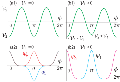
Figure 2: (a1) Potential energy as a function of $\phi$, where there are two minima at $\phi=0$ and $\pi$; (a2) wave functions as a function of $\phi$, where the magenta curve indicates the symmetric ground state $\psi_{+}$ and the cyan curve indicates the antisymmetric first-excited state $\psi_{-}$. Here, we have set $\mathcal{V}_{1}=0$ and $\mathcal{V}_{2}=20$. (a2) Potential energy as a function of $\phi$, where there is only one minimum at $\phi=0$; (b2) wave functions as a function of $\phi$, where the magenta curve indicates the eigenfunction $\psi_{0}$ of the state $|0\rangle$ and the cyan curve indicates $\psi_{1}$ of $|1\rangle$. Here, we have set $\mathcal{V}_{1}=1$ and $\mathcal{V}_{2}=20$.

The eigenequation $\mathcal{H}\psi=\varepsilon\psi$ reads

$$\left[\frac{d^{2}}{d\phi^{2}}+\mathcal{V}_{2}\cos 2\phi+\mathcal{V}_{1}\cos\phi\right]\psi=-\varepsilon\psi.$$ (11)

This is the Whittaker–Hill equation, which is reduced to the Mathieu equation for $\mathcal{V}_{1}=0$.

II.3 Strong potential limit

As the basic picture of the present model, we require the dominant role of the cosine potential $\cos 2\phi$ to generate two-fold degenerated ground states at $\phi=0$ and $\pi$, which we regard to form one-qubit states {$|0\rangle,|1\rangle$}. On the other hand, we use the cosine potential $\cos\phi$ to make gate operations. Hence, we consider the regime where $\mathcal{V}_{2}\gg\mathcal{V}_{1}\geq 0$. It is possible to derive the analytical solutions around these two points for sufficiently large $\mathcal{V}_{2}$. The Whittaker-Hill equation (11) is approximated as

$$\left[\frac{d^{2}}{d\phi^{2}}+\left(\mathcal{V}_{2}+\left(-1\right)^{q}\mathcal{V}_{1}\right)-\left(2\mathcal{V}_{2}+\left(-1\right)^{q}\frac{\mathcal{V}_{1}}{2}\right)\phi_{q}^{2}\right]\psi_{q}$$

$$\hskip 113.81102pt=\varepsilon_{q}\psi_{q},$$ (12)

where $\phi_{q}=\phi-q\pi$ with $q=0,1$.

By solving Eq.(12), the wave function $\psi_{q}$ is given by

$$\psi_{q}\left(\phi_{q}\right)=\left(\frac{2a}{\pi}\right)^{1/4}e^{-\alpha_{q}\phi_{q}^{2}},$$ (13)

with

$$\alpha_{q}=\sqrt{\frac{\mathcal{V}_{2}}{2}+\left(-1\right)^{q}\frac{\mathcal{V}_{1}}{8}}.$$ (14)

The energy of the state (13) is

$$\varepsilon_{q}=-\left(\mathcal{V}_{2}+\left(-1\right)^{q}\mathcal{V}_{1}\right)+\sqrt{2\mathcal{V}_{2}+\left(-1\right)^{q}\frac{\mathcal{V}_{1}}{2}}.$$ (15)

When $\mathcal{V}_{1}>0$, the ground state is given by $\psi_{0}$, and the first excited state by $\psi_{1}$. The wave function $\psi_{q}$ describes the one-qubit state $|q\rangle$ with the qubit variable $q=0,1$.

When $\mathcal{V}_{1}=0$, these two states are degenerate. However, an energy splitting occurs due to the difference between the Whittaker-Hill equation (11) and the approximated equation (12). Then, due to the mixing, the ground state and the first-excited state wave functions turn out to be the symmetric function $\psi_{+}$ and the antisymmetric function $\psi_{-}$,

$$\psi_{+}=\frac{\psi_{0}+\psi_{1}}{\sqrt{2}},\quad|\psi_{-}\rangle\equiv\frac{\psi_{0}-\psi_{1}}{\sqrt{2}},$$ (16)

however small the energy splitting is.

II.4 Numerical analysis

The Whittaker–Hill equation is solved by making a Fourier series expansion,

$$\psi=\sum_{n=-\infty}^{\infty}\alpha_{n}e^{in\phi}.$$ (17)

The coefficient $\alpha_{n}$ is determined by solving a set of eigenequations,

$$-n^{2}\alpha_{n}+\frac{\mathcal{V}_{2}}{2}\left(\alpha_{n+2}+\alpha_{n-2}\right)+\frac{\mathcal{V}_{1}}{2}\left(\alpha_{n+1}+\alpha_{n-1}\right)=\varepsilon\alpha_{n}.$$ (18)

This is summarized in the matrix form,

$$\sum_{m}M_{nm}\alpha_{m}=\varepsilon\alpha_{n}.$$ (19)

We have numerically solved this matrix equation by introducing a cut off as in

$$\psi=\sum_{n=-N}^{N}\alpha_{n}e^{in\phi},$$ (20)

with a certain integer $N$. We have checked that it is enough to take $N=8$. Here we use $N=12$.

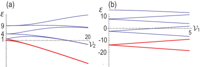
Figure 3: (a) Eigenenergy $\varepsilon$ as a function of $\mathcal{V}_{2}$ by setting $\mathcal{V}_{1}=0$. (b) Eigenenergy $\varepsilon$ as a function of $\mathcal{V}_{1}$ by setting $\mathcal{V}_{2}=20$. The lowest two energy levels are colored in red, while the other energy levels are colored in blue.

We show the energy spectrum as a function of $\mathcal{V}_{2}$ by setting $\mathcal{V}_{1}=0$ in Fig.3(a). We are concerned about the lowest two energy levels indicated in red, which are well separated from all the other. The energy is two-fold degenerated in the limit of $\mathcal{V}_{2}\rightarrow\infty$. Their wave functions are given by the symmetric function $\psi_{+}$ and the antisymmetric function $\psi_{-}$, as shown in Fig.2(a2).

We show the energy spectrum as a function of $\mathcal{V}_{1}$ by setting $\mathcal{V}_{2}=20$ in Fig.3(b). The almost two-fold degenerated energy levels split linearly as a function of $\mathcal{V}_{1}$. The ground state and the first-excited state wave functions are $\psi_{0}$ and $\psi_{1}$, which are localized at $\phi=0$ and $\pi$, as shown in Fig.2(b2) for the case of $\mathcal{V}_{2}=20$ and $\mathcal{V}_{1}=1$.

II.5 Quantum tunneling

We use the two states $\left|0\right\rangle$ and $\left|1\right\rangle$ as the one-qubit states. Because these two states are degenerate when $\mathcal{V}_{1}=0$, one may wonder if they are naturally mixed by quantum tunneling. Then, the life time of a qubit state is too short. However, this is not the case. During gate operations we keep $\mathcal{V}_{2}$ quite large to keeps the cosine potential well defined, as generates a quite large barrier between these two states.

Quantum tunneling is estimated by means of the WKB approximation. The tunneling rate $\Gamma$ is given by

$$\Gamma=e^{-2\gamma},\quad\gamma\equiv\frac{1}{\hbar}\int_{0}^{\pi}d\phi\left|\sqrt{2\mu r^{2}\left(\mathcal{V}_{2}+\mathcal{V}_{2}\left(\phi\right)\right)}\right|.$$ (21)

By setting $\mathcal{V}_{2}\left(\phi\right)=-\mathcal{V}_{2}\cos 2\phi$, we find

$$\gamma=\frac{4\sqrt{\mu r^{2}\mathcal{V}_{2}}}{\hbar}.$$ (22)

Hence, the quantum tunneling is exponentially small as a function of the applied voltage $V_{2}$. It is estimated that $\gamma=10^{6}\sim 10^{8}$ for $V_{2}=$1mV$\sim$100mV, where we have used that the inertia $\mu r^{2}$ is 10^-30kgm²[38]. See Sec.IV with respect to these parameters.

III Qubit operations

III.1 Initialization

The present system is composed of a chain of nanotube rotators, each of which is subject to the cosine potential $\cos 2\phi_{n}$ as in Fig.2(a1) by requiring $\mathcal{V}_{1}=0$. The ground states are $N$-qubit states $\left|q_{1}q_{2}\cdots q_{N}\right\rangle$ with $q_{n}=0,1$ for $n=1,2,\cdots,N$. The initialization to the state $\left|00\cdots 0\right\rangle$ is necessary for quantum computations. It is done by the annealing method. First, we start with a high temperature, where the rotational angle is random. Then, we cool down the sample slowly by applying a voltage $\mathcal{V}_{1}$ to all the outer plates in the right-hand side of the rotators. The rotators tend to the angle $\phi_{n}=0$ in order to minimize the electrostatic energy. As a result, all of the rotators have the angle $\phi_{n}=0$, which corresponds to the state $\left|00\cdots 0\right\rangle$.

III.2 One-qubit gates

We construct quantum gates for universal quantum computations. It is enough to design the arbitrary phase-shift gate and the NOT gate with respect to one-qubit gates. These gates are realized by varying the parameters $\mathcal{V}_{1}$ and $\mathcal{V}_{2}$ in the potential (8). We investigate the quantum dynamics governed by

$$i\frac{d}{d\tau}\psi\left(\phi,\tau\right)=\mathcal{H}\left(\tau\right)\psi\left(\phi,\tau\right),$$ (23)

or equivalently,

$$i\frac{d}{d\tau}\alpha_{n}\left(\tau\right)=\sum_{m}M_{nm}\left(\tau\right)\alpha_{m}\left(\tau\right),$$ (24)

in terms of the coefficients $\alpha_{n}$ in Eq.(17). We numerically solve these differential equations in the following.

In the present instance, we assume that either $\mathcal{V}_{1}$ or $\mathcal{V}_{2}$ is time dependent during a gate operation. We consider a quantum gate operation satisfying

$$\mathcal{H}(\tau_{\text{final}})=\mathcal{H}(\tau_{\text{initial}}).$$ (25)

Namely, we tune so that $\mathcal{V}_{2}(\tau_{\text{final}})=\mathcal{V}_{2}(\tau_{\text{initial}})$ and $\mathcal{V}_{1}(\tau_{\text{final}})=\mathcal{V}_{1}(\tau_{\text{initial}})$. Then, the wave function after the gate operation is expanded by the superposition of the two gaussian functions (13), which enables us to determine the coefficients of $\left|0\right\rangle$ and $\left|1\right\rangle$.

This process is represented by a unitary matrix $U$ from the initial state $(\left|0\right\rangle_{\text{initial}},\left|1\right\rangle_{\text{initial}})$ to the final state $(\left|0\right\rangle_{\text{final}},\left|1\right\rangle_{\text{final}})$ defined by

$$\left(\begin{array}[]{c}\left|0\right\rangle_{\text{final}}\\ \left|1\right\rangle_{\text{final}}\end{array}\right)=U\left(\begin{array}[]{c}\left|0\right\rangle_{\text{initial}}\\ \left|1\right\rangle_{\text{initial}}\end{array}\right).$$ (26)

This unitary matrix defines a one-qubit gate.

III.3 Phase-shift gate

We construct the arbitrary phase-shift gate defined by

$$U_{Z}(\theta)\equiv\text{diag.}(1,e^{i\theta}),$$ (27)

whose action is

$$U_{Z}(\theta)\left|0\right\rangle=\left|0\right\rangle,\qquad U_{Z}(\theta)\left|1\right\rangle=e^{i\theta}\left|1\right\rangle.$$ (28)

As is well known, time evolution generates a phase to a state according to the Schrödinger equation. Hence, the two states $|0\rangle$ and $|1\rangle$ acquire different phases as time evolves, provided their energies are made different by the presence of $\mathcal{V}_{1}$. This is the basic idea of the phase-shift gate.

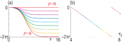
Figure 4: (a) Time evolution of phase modulation. We have set $\tau_{1}=4$ and $\tau_{2}-\tau_{1}=0.41p$ with $p=0,1,\cdots,8$. (b) Phase modulation as a function of $\tau_{2}$, where $4\leq\tau_{2}\leq 8$. We have set $\mathcal{V}_{2}=20$, $\mathcal{V}_{1}=1$, $\mathcal{T}=2$ and $T=10$.

We temporary control $\mathcal{V}_{1}$ by tuning an applied voltage difference according to the formula

$$\mathcal{V}_{1}\left(\tau\right)=\frac{\mathcal{\bar{V}}_{1}}{2}\left[\tanh\frac{\tau-\tau_{2}}{\mathcal{T}}-\tanh\frac{\tau-\tau_{1}}{\mathcal{T}}+2\right],$$ (29)

with $\tau_{2}\gg\tau_{1}$, while we fix $\mathcal{V}_{2}\neq 0$. We start either from the state $|0\rangle$ or $|1\rangle$. The absolute value of the wave function does not change its form but only the phase rotation is modulated because the state remains in the bottom of the cosine potential. We show the phase modulation as a function of time for various $\tau_{2}$ in Fig.4(a). The phase difference between the initial state and the final state is shown in Fig.4(b), which is linear as a function of $\tau_{2}-\tau_{1}$. The phase modulations between the two states $|0\rangle$ and $|1\rangle$ are opposite as in

$$U_{\theta}\equiv\text{diag.}(e^{-i\theta/2},e^{i\theta/2}),$$ (30)

because the energy splitting is opposite between them. Here,

$$\theta/2\pi=\mathcal{\bar{V}}_{1}f(\mathcal{V}_{2})(\tau_{2}-\tau_{1}).$$ (31)

We find $f(\mathcal{V}_{2})=-0.3$ in the case of $\mathcal{V}_{2}=20$ by fitting the line in Fig.4(b). This is equivalent to the phase-shift gate (27), because the overall phase is irrelevant to quantum gate operations.

III.4 $\pi/4$ phase-shift gate

The $\pi/4$ phase-shift gate

$$U_{T}\equiv\text{diag.}(1,e^{i\pi/4})$$ (32)

is realized by setting $\theta=\pi/4$ in the generic phase-shift gate (27).

III.5 Pauli-Z gate

The Pauli-Z gate is realized by the $z$ rotation with the angle $\pi$ as

$$U_{Z}=-iU_{Z}\left(\pi\right)$$ (33)

in the generic phase-shift gate (27).

III.6 NOT gate

We construct the NOT gate defined by

$$U_{\text{NOT}}\equiv\left(\begin{array}[]{cc}0&1\\ 1&0\end{array}\right).$$ (34)

This gate exchanges the two states $|0\rangle$ and $|1\rangle$. It is impossible to keep the potential $\mathcal{V}_{2}$ finite since it prohibits quantum tunneling.

For this purpose we temporary control $\mathcal{V}_{2}$ by tuning the applied voltage to the rotator in such a way that

$$\mathcal{V}_{2}\left(\tau\right)=\frac{\mathcal{\bar{V}}_{2}}{2}\left[\tanh\frac{\tau-\tau_{2}}{\mathcal{T}}-\tanh\frac{\tau-\tau_{1}}{\mathcal{T}}+2\right],$$ (35)

with $\tau_{2}\gg\tau_{1}$, while we set $\mathcal{V}_{1}=0$. The gate operation requires that the initial state $|0\rangle$ is transferred to the final state $|1\rangle$ as in Fig.5(c). We explain how to obtain this time evolution. Let its time evolution be described by the wave function $\psi(\phi,\tau)$. The initial condition implies that it satisfies $\psi(0,\tau)=\psi_{\text{max}}$ and $\psi(\pi,\tau)=0$ at $\tau=0$, where $\psi_{\text{max}}$ is the maximum value of $|\psi(\phi,\tau)|$. The final state should satisfies $\psi(0,\tau)=0$ and $\psi(\pi,\tau)=\psi_{\text{max}}$ at $\tau=T\gg\tau_{2}$, because $|0\rangle$ is transformed to the state $|1\rangle$.

This is a nontrivial problem depending on the parameters $\tau_{2}$ in the applied voltage $\mathcal{V}_{2}\left(\tau\right)$. We fix $\tau_{1}$ arbitrarily and solve the Schrödinger equation for $\psi(\phi,T)$ as a function of $\tau_{2}$, whose result we show in Fig.5(a). There is a certain value of $\tau_{2}$ where $|\psi(0,T)|=0$ and $|\psi(\pi,T)|=\psi_{\text{max}}$, as is clear in Fig.5(b). Then, we show the dynamics of $|\psi(\phi,\tau)|$ with the use of this value of $\tau_{2}$ in Fig.5(c) and (d), where it is seen that the initial state $|0\rangle$ localized at $\phi=0$ is transformed to the final state $|1\rangle$ localized at $\phi=\pm\pi$. This is the action of the NOT gate.

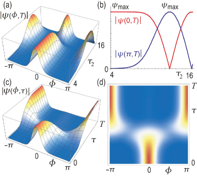
Figure 5: Time evolution of the NOT gate operation. (a) Bird’s eye’s view of the final state $|\psi(\phi,T)|$ as a function of $\phi$ and $\tau_{2}$, where $-\pi\leq\phi<\pi$ and $4\leq\tau_{2}\leq 16$. (b) The final state $|\psi(0,T)|$ colored in red and $|\psi(\pi,T)|$ colored in blue as a function of $\tau_{2}$, where $4\leq\tau_{2}\leq 16$. (c) Bird’s eye’s view of $|\psi(\phi,\tau)|$, where $-\pi\leq\phi<\pi$ and $0\leq\tau<T$. (d) Top view of $|\psi(\phi,\tau)|$. We have set $\mathcal{\bar{V}}_{2}=20$, $\mathcal{V}_{1}=0$, $\tau_{1}=4$, $\mathcal{T}$ $=2$ and $T=20$ in (a) and (b). We have additionally set $\tau_{2}=12.6$ in (c) and (d).

III.7 Hadamard gate

The Hadamard gate is defined by

$$U_{\text{H}}\equiv\frac{1}{\sqrt{2}}\left(\begin{array}[]{cc}1&1\\ 1&-1\end{array}\right).$$ (36)

It is realized by a sequential application of the Pauli Z gates and the NOT gate [35] as

$$U_{\text{H}}=-iU_{Z}U_{\text{NOT}}U_{Z}.$$ (37)

III.8 Two-qubit gates

A two-qubit system is made of two rotators put along the $x$ axis as in Fig.1. The two-qubit state is expressed as $\left|q_{1}q_{2}\right\rangle$ with $q_{n}=0,1$. An example of the state $\left|01\right\rangle$ is given in the system made of Fig.1(b3) and (c3). A two-qubit gate operation transforms the initial state $\left|q_{1}q_{2}\right\rangle_{\text{initial}}$ to the final state $\left|q_{1}q_{2}\right\rangle_{\text{final}}$ as

$$\left(\begin{array}[]{c}\left|00\right\rangle_{\text{final}}\\ \left|01\right\rangle_{\text{final}}\\ \left|10\right\rangle_{\text{final}}\\ \left|11\right\rangle_{\text{final}}\end{array}\right)=U\left(\begin{array}[]{c}\left|00\right\rangle_{\text{initial}}\\ \left|01\right\rangle_{\text{initial}}\\ \left|10\right\rangle_{\text{initial}}\\ \left|11\right\rangle_{\text{initial}}\end{array}\right),$$ (38)

which defines the two-qubit gate operation $U$.

III.9 Two-qubit phase-shift gate

We apply the voltage difference $V_{12}$ between the two rotators as in Fig.1(b3) and (c3). The potential energy is given by

$$W\left(\phi_{1},\phi_{2}\right)\equiv W_{2}\left(\phi_{1}\right)+W_{2}\left(\phi_{2}\right)+\frac{C\left(\phi_{1},\phi_{2}\right)}{2}V_{12}^{2},$$ (39)

where $W_{2}\left(\phi\right)$ is the potential energy given by Eq.(1), and $C(x_{1},x_{2})$ is the capacitance between the rotators,

$$C(\phi_{1},\phi_{2})=\frac{\varepsilon_{0}S}{L\left(\phi_{1},\phi_{2}\right)}.$$ (40)

Here, $\varepsilon_{0}$ and $S$ are the permittivity and the area of the plates, while $L\left(\phi_{1},\phi_{2}\right)$ is the distance between the two plates attached to the rotator.

When we apply the Ising gate, the absolute values of the wave functions do not change but only the phases are modulated. The wave functions are $|0\rangle$ or $|1\rangle$, and hence we concentrate on the parallel case $\phi_{1},\phi_{2}=0,\pi$. There are relations,

$$L\left(0,0\right) =L\left(\pi,\pi\right)=\ell,$$ (41)

$$L\left(0,\pi\right) =2R+\ell,\quad L\left(\pi,0\right)=-2R+\ell,$$ (42)

where $R$ is the radius of the rotation of the rotator, and $\ell$ is the length between the supporting points of two adjacent rotators: See Fig.1(b3) and (c3).

We calculate

$$W\left(0,0\right) =W\left(\pi,\pi\right)=\frac{\varepsilon_{0}S}{\ell}\frac{V_{12}^{2}}{2}\equiv E_{0},$$ (43)

$$W\left(0,\pi\right) =\frac{\varepsilon_{0}S}{\ell+2R}\frac{V_{12}^{2}}{2}\equiv E_{+},$$ (44)

$$W\left(\pi,0\right) =\frac{\varepsilon_{0}S}{\ell-2R}\frac{V_{12}^{2}}{2}\equiv E_{-}.$$ (45)

We show that the potential energy (39) may be written in the form of the Ising model with field $B_{j}$,

$$H_{\text{Ising}}=\sum_{j=1}^{N-1}J_{j}s_{j}s_{j+1}+\sum_{j=1}^{N}B_{j}s_{j}+E_{0},$$ (46)

where $s_{j}=\pm 1$. We rewrite Eq.(46) as

$$H_{\text{Ising}}=\sum_{j=1}^{N-1}H_{j}\left(s_{j},s_{j+1}\right)+\frac{B_{1}}{2}s_{1}+\frac{B_{N}}{2}s_{N},$$ (47)

with

$$H_{j}\left(s_{j},s_{j+1}\right)=J_{j}s_{j}s_{j+1}+\frac{B_{j}}{2}s_{j}+\frac{B_{j+1}}{2}s_{j+1}+\frac{E_{0}}{N-1}.$$ (48)

We realize the term (48) by a system made of two adjacent buckled plates $j$ and $j+1$. There are relations

$$H_{j}\left(1,1\right) =W\left(0,0\right),\qquad H_{j}\left(-1,-1\right)=W\left(\pi,\pi\right),$$ (49)

$$H_{j}\left(1,-1\right) =W\left(0,\pi\right),\qquad H_{j}\left(-1,1\right)=W\left(\pi,0\right).$$ (50)

The coefficients in the Ising model are given by

$$J_{j} =\frac{2E_{0}-E_{+}-E_{-}}{4},$$ (51)

$$B_{j} =-B_{j+1}=\frac{E_{+}-E_{-}}{4},$$ (52)

$$E_{0} =\frac{2E_{0}+E_{+}+E_{-}}{4}.$$ (53)

We start with the Gaussian state $\Psi_{\sigma_{1}\sigma_{2}}\left(x_{1},x_{2}\right)\equiv\psi_{\sigma_{1}}(x_{1})\psi_{\sigma_{2}}(x_{2})$ with Eq.(13) localized at four points $x_{1}=\sigma_{1}R$ and $x_{2}=\sigma_{2}R$, where $\sigma_{1}=\pm,\sigma_{2}=\pm$. The absolute value of this wave function almost remains as it is, but a phase shift occurs. The unitary evolution is given by

$$U\left(t\right)=\exp[-i\left(E_{0}/\hbar+\omega\right)t]$$ (54)

for $\sigma_{1}=\sigma_{2}=+$ and $\sigma_{1}=\sigma_{2}=-$,

$$U\left(t\right)=\exp[-i\left(E_{+}/\hbar+\omega\right)t]$$ (55)

for $\sigma_{1}=+$ and $\sigma_{2}=-$,

$$U\left(t\right)=\exp[-i\left(E_{-}/\hbar+\omega\right)t]$$ (56)

for $\sigma_{1}=-$ and $\sigma_{2}=+$, where we have added the zero-point energy.

It corresponds to the two-qubit phase-shift gate operation,

$$U_{\text{2-phase}}\left(t\right) =\text{diag.}\left(e^{-i\frac{E_{0}}{\hbar}t},e^{-i\frac{E_{-}}{\hbar}t},e^{-i\frac{E_{+}}{\hbar}t},e^{-i\frac{E_{0}}{\hbar}t}\right)$$

$$=e^{-i\frac{E_{0}}{\hbar}t}\text{diag.}\left(1,e^{-i\frac{E_{X}}{\hbar}t},e^{i\frac{E_{X}}{\hbar}t},1\right),$$ (57)

by identifying the qubit state $\left(\left|00\right\rangle,\left|01\right\rangle,\left|10\right\rangle,\left|11\right\rangle\right)^{t}=\left(\left|++\right\rangle,\left|+-\right\rangle,\left|-+\right\rangle,\left|--\right\rangle\right)^{t}$.

III.10 Ising gate

The Ising gate is defined by $U_{ZZ}\equiv$diag.$(1,-1,-1,1)$, and realized by setting $E_{X}t/\hbar=\pi$ in Eq.(57) up to the global phase $\exp\left[-iE_{0}t/\hbar\right]$.

III.11 CZ gate

The controlled-Z (CZ) gate is defined by $U_{\text{CZ}}=$diag.$(1,1,1,-1)$. It is constructed by a sequential application of the Ising gate and the one-qubit phase-shift gates as[36]

$$U_{\text{CZ}}=e^{i\pi/4}U_{Z}\left(\frac{\pi}{2}\right)U_{Z}\left(\frac{\pi}{2}\right)U_{ZZ}.$$ (58)

III.12 CNOT gate

The CNOT is defined by

$$U_{\text{CNOT}}^{1\rightarrow 2}\equiv\left(\begin{array}[]{cccc}1&0&0&0\\ 0&1&0&0\\ 0&0&0&1\\ 0&0&1&0\end{array}\right),$$ (59)

and is constructed by a sequential application of the CZ gate (58) and the Hadamard gate $U_{\text{H}}^{\left(2\right)}$ in Eq.(37) acting on the second qubit as $U_{\text{CNOT}}^{1\rightarrow 2}=U_{\text{H}}^{\left(2\right)}U_{\text{CZ}}U_{\text{H}}^{\left(2\right)}$.

III.13 Readout process

The readout of the plate angle $\phi_{n}$ can be done for all rotators by using the fact that the capacitance depends on the relative angle of the two plates[27]. By applying a tiny voltage and by measuring the induced current, we can readout the capacitance, which is directly related to the angle $\phi_{n}$.

IV Discussion

We have proposed a universal quantum computer with the use of a chain of carbon nanotubes together with metal plates attached to them. One-qubit gate operations are controlled electrically by giving voltage difference between the attached plate and other plates fixed to the outer system. Two-qubit operations are controlled electrically by given voltage difference between the two attached plates belonging to two adjacent nanotubes. We now discuss the feasibility of such a quantum computer.

We mention experimentally obtained material parameters of a double-wall nanotube structure[29]. Nanotube length is 10nm and the intertube gap length is 0.3nm. The diameter of a nanotube is 10nm[22]. Q factor[37] is of the order of 100. The inertia $\mu r^{2}$ is 10^-30kgm²[38]. The rotational frequency is from 1MHz[37] to 100GHz[29].

If we use a plate with 10nm square with the distance $L=100$nm, the capacitance $C=\varepsilon_{0}S/L$ is 10^-21F. If we apply 1mV to the plate, the electrostatic energy $CV^{2}/2$ is 10^-26Nm and the operating time is of the order of 10$\mu$s. If we apply 100mV to the plates, the electrostatic energy is 10^-22Nm and the operating time is of the order of 1ns. These values are experimentally feasible.

This work is supported by CREST, JST (Grants No. JPMJCR20T2).

References

- [1] R. Feynman, Simulating physics with computers, Int. J. Theor. Phys. 21, 467 (1982).
- [2] D. P. DiVincenzo, Quantum Computation, Science 270, 255 (1995).
- [3] M. Nielsen and I. Chuang, "Quantum Computation and Quantum Information", Cambridge University Press, (2016); ISBN 978-1-107-00217-3.
- [4] Y. Nakamura; Yu. A. Pashkin; J. S. Tsai, Coherent control of macroscopic quantum states in a single-Cooper-pair box, Nature 398, 786 (1999).
- [5] E. Knill, R. Laflamme and G. J. Milburn, A scheme for efficient quantum computation with linear optics, Nature, 409, 46 (2001).
- [6] J. I. Cirac and P. Zoller, Quantum Computations with Cold Trapped Ions, Phys. Rev. Lett. 74, 4091 (1995).
- [7] L. M.K. Vandersypen, M. Steffen, G. Breyta, C. S. Yannoni, M. H. Sherwood, I. L. Chuang, Nature 414, 883 (2001).
- [8] B. E. Kane, Nature 393, 133 (1998).
- [9] D. Loss and D. P. DiVincenzo, Quantum computation with quantum dots, Phys. Rev. A 57, 120 (1998).
- [10] C. Psaroudaki and C. Panagopoulos, Phys. Rev. Lett. 127, 06720 (2021).
- [11] J. Xia, X. Zhang, X. Liu, Y. Zhou, M. Ezawa, arXiv:2204.04589
- [12] J. Xia, X. Zhang, X. Liu, Y. Zhou, M. Ezawa, Commun. Mater. 3, 88 (2022).
- [13] S. Rips and M. J. Hartmann, Phys. Rev. Lett. 110, 120503 (2013).
- [14] S. Rips, I. Wilson-Rae and M. J. Hartmann, Phys. Rev. A 89, 013854 (2014).
- [15] F. Pistolesi, A. N. Cleland, and A. Bachtold, Phys. Rev. X 11, 031027 (2021).
- [16] M. Ezawa, S. Yasunaga, A. Higo, T. Iizuka, Y. Mita, arXiv:2208.04528
- [17] D. Deutsch, Quantum theory, Proceedings of the Royal Society A. 400, 97 (1985).
- [18] C. M. Dawson and M. A. Nielsen, quant-ph/arXiv:0505030.
- [19] M. Nielsen and I. Chuang, "Quantum Computation and Quantum Information", Cambridge University Press, Cambridge, UK (2010).
- [20] H. G. Craighead, Science 290, 1532 (2000).
- [21] K. L. Ekinci and M. L. Roukes, Rev. Sci. Instruments 76, 6 (2005).
- [22] A. M. Fennimore, T. D. Yuzvinsky, W.-Q. Han, M. S. Fuhrer, J. Cumings and A. Zettl, Nature 424, 408 (2003).
- [23] A. Barreiro, R. Rurali, E. R. Herndez, J. Moser, T. Pichler, L. Forro A. Bachtold, Science 320 (5877): 775 (2008).
- [24] K. Cai, J. Wan, Q. H. Qin and J. Shi, Nanotechnology 27, 055706 (2016).
- [25] K. Cai, J. Yu, J. Wan, H. Yin, J. Shi, Q H. Qin, Carbon, 101, 168 (2016).
- [26] A. N. Kolmogorov and V. H. Crespi, Phys. Rev. Lett. 85, 4727 (2000).
- [27] B. Bourlon, D. C. Glattli, C. Miko, L. Forr and A. Bachtold, Nano Lett. 4, 709 (2004).
- [28] Z. Xu, Q.-S. Zheng and G. Chen, Phys. Rev. B 75, 195445 (2007).
- [29] K. Cai, Y. Li, Q. H. Qin and H. Yin, Nanotechnology 25, 505701 (2014).
- [30] H. A. Zambrano, J. H. Walther and R. L. Jaffe, J. Chem. Phys. 131 (24) 241104 (2009).
- [31] R. Saito, Physical Properties of Carbon Nanotubes, Imperial College Press (1998)
- [32] M. Blencowe, Physics Reports 395, 159 (2004).
- [33] M. Poot, H. S.J. van der Zant, Physics Reports 511, 273 (2012.)
- [34] O. Slowik, K. Orlowska, D. Kopiec, P. Janus, P. Grabiec and T. Gotszalk, Measurement Automation Monitoring, Mar., 62, 2450 (2016).
- [35] N. Schuch and J. Seiwert, Phys. Rev. A 67, 032301 (2003).
- [36] Y. Makhlin, Quant. Info. Proc. 1, 243 (2002).
- [37] S.J. Papadakis, A.R. Hall, P. A.Williams, L.Vicci, M.R. Falvo, R. Superfine and S.Washburn, Phys. Rev. Lett. Phys. Rev. Lett. 93, 146101 (2004).
- [38] T. D. Yuzvinsky, A. M. Fennimore, A. Kis and A. Zettl, Nanotechnology 17, 434 (2006)