Abstract

Tidal disruption events (TDEs) around super massive black holes (SMBHs) are a potential laboratory to study super-Eddington accretion disks and sometimes result in powerful jets or outflows which may shine in the radio and sub millimeter bands. In this work, we model the thermal synchrotron emission of jets from general relativistic radiation magneto-hydrodynamics (GRRMHD) simulations of a BH accretion disk/jet system which assumes the TDE resulted in a magnetized accretion disk around a BH accreting at $\sim 12-25$ times the Eddington accretion rate. Through synthetic observations with the Next Generation Event Horizon Telescope (ngEHT) and an image reconstruction analysis, we demonstrate that TDE jets may provide compelling targets, within the context of the models explored in this work. In particular, we find that jets launched by a SANE super-Eddington disk around a spin $a_{*}=0.9$ reach the ngEHT detection threshold at large distances (up to 100 Mpc in this work). A two-temperature plasma in the jet or weaker jets, such as a spin $a_{*}=0$ model, requires a much closer distance as we demonstrate detection at 10 Mpc for limiting cases of $a_{*}=0,\,\mathcal{R}=1$ or $a_{*}=0.9,\,\mathcal{R}=20$. We also demonstrate that TDE jets may appear as superluminal sources if the BH is rapidly rotating and the jet is viewed nearly face on.

1 1 0 https://doi.org/ Modeling Reconstructed Images of Jets Launched by SANE Super-Eddington Accretion Flows Around SMBHs with the ngEHT Modeling Reconstructed Images of Jets Launched by SANE Super-Eddington Accretion Flows Around SMBHs with the ngEHT Brandon Curd^1,2,∗, Razieh Emami ², Freek Roelofs^1,2 and Richard Anantua ³ Brandon Curd, Razieh Emami, Freek Roelofs and Richard Anantua Curd, B. et al., Correspondence: brandon.curd@cfa.harvard.edu

1 Introduction

Tidal disruptions of stars by super massive black holes (SMBHs), or tidal disruption events (TDEs), have recently become a regularly observed transient phenomenon. Stars which enter the tidal radius

$$R_{t}\simeq 7\times 10^{12}\left(\dfrac{M_{\rm{BH}}}{10^{6}M_{\odot}}\right)^{1/3}\left(\dfrac{M_{*}}{M_{\odot}}\right)^{-1/3}\left(\dfrac{R_{*}}{R_{\odot}}\right)\rm{[cm]}$$ (1)

of the central SMBH in their host galaxy will be disrupted Hills (1975); Rees (1988), either partially or fully depending on the orbit and equation of state of the star Guillochon and Ramirez-Ruiz (2013); Mainetti et al. (2017). The bound stream of gas returns towards the BH delivering mass at the fallback rate ($\dot{M}_{\rm{fb}}$). Apsidal precession of the returning stream leads to self-intersection with material that has yet to pass through pericenter and leads to dissipation and disk formation. Dissipation due to self-intersection may also be a source of early emission in a TDE Steinberg and Stone (2022). After the initial rise to peak, the fallback rate follows a power law behaviour which can be approximated as

$$\dot{M}_{\rm{fb}}=\dot{M}_{\rm{fb,peak}}\left(\dfrac{t}{t_{\rm{fb}}}\right)^{-5/3}.$$ (2)

Here $\dot{M}_{\rm{fb,peak}}$ is the peak mass fallback rate

$$\dfrac{\dot{M}_{\rm{fb,peak}}}{\dot{M}_{\rm{Edd}}}\approx 133\left(\dfrac{M_{\rm{BH}}}{10^{6}M_{\odot}}\right)^{-3/2}\left(\dfrac{M_{*}}{M_{\odot}}\right)^{2}\left(\dfrac{R_{*}}{R_{\odot}}\right)^{-3/2}$$ (3)

making the “frozen in” approximation as in Stone et al. (2013), and

$$t_{\rm{fb}}=3.5\times 10^{6}\,{\rm{s}}\,\left(\dfrac{M_{\rm{BH}}}{10^{6}M_{\odot}}\right)^{1/2}\left(\dfrac{M_{*}}{M_{\odot}}\right)^{-1}\left(\dfrac{R_{*}}{R_{\odot}}\right)^{3/2},$$ (4)

is the fallback time, which is the orbital time of the most bound part of the stream. Of note is the fact that the mass fallback rate can greatly exceed the Eddington mass accretion rate $\dot{M}_{\rm{Edd}}$. The exact power law behaviour varies with the properties and orbit of the star Golightly et al. (2019).

TDEs are typically seen as optical/X-ray transients Komossa (2015); Gezari (2021), but several TDEs have resulted in outflows or jets which shine in the radio bands Alexander et al. (2020). In the most common case in which no relativistic jet is launched (commonly referred to as “non-jetted” TDEs), the X-ray and optical/UV luminosity follows a roughly $t^{-5/3}$ decline, similar to the fallback rate. If the TDE leads to prompt disk formation, the X-rays are thought to arise from an accretion disk while the optical/UV emission arises from a large scale reprocessing layer Dai et al. (2018); Curd et al. (2022). TDEs have also been observed to launch relativistic X-ray jets in a few cases. These jetted TDEs have been argued to arise due to a magnetically arrested disk (MAD, Gammie et al., 2003) forming around the BH during the TDE Tchekhovskoy et al. (2014); Dai et al. (2018); Curd and Narayan (2019), which leads to jet production via the Blandford-Znajek mechanism Blandford and Znajek (1977) extracting spin energy from the BH. Alternatively, jets may be produced thanks to radiative acceleration of gas through a narrow funnel region Coughlin and Begelman (2020).

A handful of non-jetted TDEs have been observed to produce radio emission peaking at tens of GHz with $L_{\rm{radio}}\sim 10^{37-39}\rm{erg\,s^{-1}}$. This emission is thought to arise from an outflow launched by the TDE with velocity $v\sim 0.1c$ shocking on the gas surrounding the BH. Meanwhile, jetted TDEs produce bright radio emission peaking at $L_{\rm{radio}}\sim 10^{40-42}\rm{erg\,s^{-1}}$. The appearance of radio emission is often delayed by several weeks from the initial appearance of the optical/UV/X-ray emission in non-jetted TDEs, which hints at some connection to the disk formation process to the occurrence of outflows.

After $\dot{M}_{\rm{fb}}$ rises to peak, it has previously been assumed that by this stage a circularized accretion disk has formed Dai et al. (2018); Curd and Narayan (2019). The first direct demonstration of circularization near the peak fallback rate was recently demonstrated in a numerical simulation by Steinberg and Stone (2022). Multiple authors have argued in favor of a picture in which an inner accretion flow is surrounded by a quasi-spherical reprocessing layer since this naturally explains the sometimes delayed appearance of X-ray emission in optical/UV discovered TDEs Dai et al. (2018); Thomsen et al. (2022); Curd et al. (2022). This picture naturally arises if the accretion flow is actually super-Eddington Dai et al. (2018), which has motivated multiple studies of GRRMHD simulations magnetized of super-Eddington disks. Motivated by this fact and the demonstration that the “standard and normal evolution” (or SANE, citation) super-Eddington accretion disk also lead to viewing angle effects which may explain the behaviour in non-jetted TDEs Curd and Narayan (2019), we conducted a study of the outflows launched by SANE models in Curd et al. (2022) and studied their radio-submm emission. We focus on these SANE models in this work as well.

The Next Generation Event Horizon Telescope (ngEHT) will provide more baseline coverage and faster response times than the previous mission. An estimate for ngEHT is to double the antenna sites Doeleman et al. (2019) of its 20 $\mu$as predecessor EHT, and thus the number of possible baseline pairs and triads of sites available for imaging jet/accretion flow/black hole systems would scale combinatorially (the number of baselines grows with the number of antennae as (N(N-1)/2). This could allow for interesting sources such as jets from nearby tidal disruption events to be imaged directly. In our previous work Curd et al. (2022), we provided the first demonstration that SANE super-Eddington accretion flows can produce radio emission which is bright enough at 230 GHz to be detected and resolved. Here we take things a step further and produce reconstructed images assuming such jets happen in the nearby universe.

The detection rate of TDEs in the optical/UV/X-ray is expected to grow rapidly once the Large Synoptic Survey Telescope comes on line Ivezić et al. (2019); Bricman and Gomboc (2020). Assuming rapid follow-up of TDEs in radio-submm bands finds detectable emission, this could provide a large number of targets for the ngEHT. As we demonstrated in Curd et al. (2022), some models produced detectable emission even at $\sim 180$ Mpc. At this distance, a conservative estimate of the volume integrated TDE rate suggests more than 200 TDEs per year assuming volumetric TDE rates based on Stone and Metzger (2016). Even at $<40$ Mpc, we estimate that several TDEs should occur per year (see Figure 2 in Curd et al. 2022) which suggests some nearby TDEs may become targets of opportunity during the ngEHT mission.

We stress that jets such as those in our first work on the subject of jets from SANE models of TDE accretion disks Curd et al. (2022) do not resemble any previously detected radio TDEs. This may suggest most, or even all, TDEs do not form accretion disks which resemble SANE models to begin with. However, the number of TDEs that have appeared in the radio-submm in the first place is extremely small as of this writing with fewer than twenty radio TDEs reported. Furthermore, magnetic fields are certainly present in the forming disk, albeit dynamically subdominant to hydrodynamic effects early in the disk formation Sadowski et al. (2016); Curd (2021). Nevertheless, it is possible that after the disk circularizes, which Steinberg and Stone (2022) suggests may take tens of days, the magnetic field builds up in a dynamo effect similar to Sadowski et al. (2016). In this case, one would almost certainly expect the magnetic field to become dynamically important, in which case a magnetized outflow may be launched as in Curd et al. (2022). TDEs continue to surprise observers in terms of the range of behaviour, so such a jet formation channel may yet be discovered.

2 Numerical Methods

2.1 GRRHMD Simulations

Throughout this work, we often use gravitational units to define length and time. In particular, we use the gravitational radius

$$r_{g}=\dfrac{GM_{\rm{BH}}}{c^{2}}$$ (5)

and the gravitational time

$$t_{g}=\dfrac{GM_{\rm{BH}}}{c^{3}},$$ (6)

where $M_{\rm{BH}}$ is the mass of the black hole (BH). We also adopt the following definition for the Eddington mass accretion rate:

$$\dot{M}_{\rm{Edd}}=\dfrac{L_{\rm{Edd}}}{\eta_{\rm NT}c^{2}},$$ (7)

where $L_{\rm{Edd}}=1.25\times 10^{38}\,(M_{\rm{BH}}/M_{\odot})\,{\rm erg\,s^{-1}}$ is the Eddington luminosity, and $\eta_{\rm{NT}}$ is the radiative efficiency of a Novikov-Thorne thin disk around a BH with spin parameter $a_{*}$ Novikov and Thorne (1973).

We conduct an imaging analysis of GRRMHD simulations presented in Curd et al. (2022). In particular, we analyze the most massive BH models m7a0.0-HR and m7a0.9-HR, which are $M_{\rm{BH}}=10^{7}\,M_{\odot}$ BHs of spin $a_{*}=0$ and $0.9$ BHs. We specify the simulation diagnostics relevant for this work in Table 1. The simulations were conducted in 2D $(r,\vartheta)$ coordinates on a $N_{r}\times N_{\vartheta}=640\times 256$ grid with added resolution near the poles to adequately resolve both the disk and jet. The radial grid cells were logarithmically spaced with a maximum domain radius of $R_{\rm{max}}=10^{5}\,r_{g}$ to capture the large scale features of the jet.

Table 1: We tabulate the mass accretion rate $\dot{M}$, jet efficiency $\eta_{\rm{jet}}\equiv L_{\rm{jet}}/\dot{M}c^{2}$ (where $L_{\rm{jet}}$ is the jet power as defined in Curd et al. (2022)), and total simulation duration $t_{\rm{sim}}$ for each KORAL simulation. Note that $\dot{M}$ and $\eta_{\rm{jet}}$ are time averaged over the final $50,000\,t_{g}$ of each simulation.

Model	$\dot{M}$	$\eta_{\rm{jet}}$	$t_{\rm{sim}}$
	($\dot{M}_{\rm{Edd}}$)		$(t_{g})$
m7a0.0-HR	12	0.24%	$83,000$
m7a0.9-HR	25	1.15%	$81,200$

On horizon scales, gas is flowing across the BH horizon in an accretion disk due to angular momentum transport driven by the magneto rotational instability. The disk is optically thick and turbulent, and gas inside of the disk is advected with the gas across the BH horizon. However, an optically thin funnel above and below the disks exists. Here, radiation can escape freely and pushes on gas, accelerating a significant outflow. In addition, the funnel is magnetized and sometimes exhibits magnetization parameter $\sigma=b^{2}/\rho c^{2}>1$, where $b$ is the magnetic field strength and $\rho$ is the mass density of the plasma. In the jet, magnetic energy is partially converted into kinetic energy as it contributes to accelerating gas into an outflow.

In both simulations, radiative and Poynting acceleration drive fast outflows. The jet reaches relativistic speeds with Lorentz factor $\gamma>5$ for model m7a0.9-HR, which is likely due to the BZ effect extracting spin energy from the BH, which may produce roughly $\sim 1$ percent of the jet efficiency even though the magnetic flux threading the black hole is well below the MAD limit. The primary sites of dissipation are the jet head and internal shocks inside of the jet. Internal shocks are due to fast and slow moving gas interacting downstream of the jet head in addition to recollimation shocks. As we show in Figure 1, this results in a hot, magnetized jet which reaches large scales ($r>30,000\,r_{g}$) by the end of the simulation. The $a_{*}=0.9$ model has a significantly more magnetized jet and also produces a more powerful jet by a significant fraction (see Table 1).

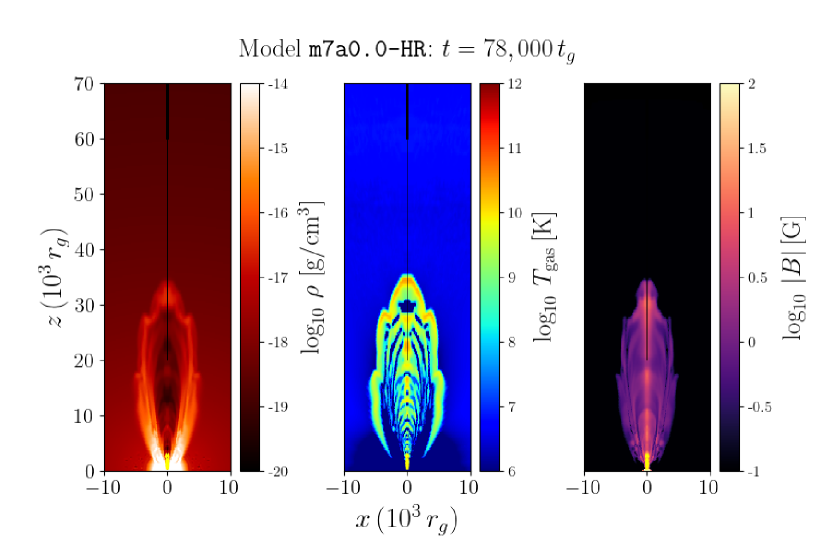
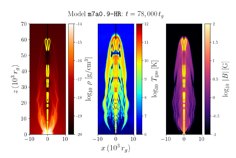
Figure 1: Here we show snapshots of the GRRMHD KORAL simulations that we post-process with ipole. All data is shown for $t=78,000\,t_{g}$ in both m7a0.0-HR (top) and m7a0.9-HR (bottom). The colors indicate the gas density $\rho$ (left), gas temperature $T_{\rm{gas}}$ (middle), and magnetic field strength $|B|$ (right) while the yellow contours indicate the $\sigma=1$ boundary, in which we set $\rho=0$ in the ray tracing step to prevent emission.

2.2 230 GHz Emission

We post-process the KORAL simulation data with the general relativistic ray tracing (GRRT) code ipole Mościbrodzka and Gammie (2018); Yarza et al. (2020); Wong et al. (2022), which includes synchrotron and Bremsstrahlung emission and absorption. The electron distribution function is assumed to be thermal. Ohmura et al. (2019, 2020) demonstrated that large scale active galactic nuclei (AGN) jets can produce a two-temperature plasma. Motivated by their findings and the possibility that a two-temperature plasma will be produced due to shocks at the jet head and within the jet itself, we test a simple two-temperature jet model by scaling the electron temperature relative to the ion temperature via the plasma temperature ratio:

$$\mathcal{R}=\dfrac{T_{i}}{T_{e}},$$ (8)

where $T_{i}$ is the temperature of the ions, and $T_{e}$ is the temperature of the electrons, respectively. Note that $T_{i}$ is obtained directly from the KORAL simulation by setting $T_{i}=T_{\rm{gas}}$.

The peak of the radio-submm spectra in m7a0.0-HR is lower than that of m7a0.9-HR, so increasing $\mathcal{R}$ has a much more significant impact on the 230 GHz emission and can make the jet undetectable even at 10 Mpc for values of $\mathcal{R}>2$ Curd et al. (2022). It is possible that a non-thermal electron distribution will have greater high energy emission even as $\mathcal{R}$ increases, but we save an exploration of non-thermal electron models for a future analysis.

Each model was imaged at $230$ GHz. For both models, we image the simulation at times $t=38,000\,t_{g}$ and $t=78,000\,t_{g}$ for a difference in observing times of $\sim 23$ days. We choose a distance $D=10$ Mpc, $\mathcal{R}=1$, observing angle relative to the jet axis ($z$ in Figure 1) of $\theta=10,45,$ and $90^{\circ}$, respectively. Note that we use $\theta$ for the observer angle while $\vartheta$ is the polar angle in the KORAL grid coordinates. For model m7a0.9-HR, we also test limiting cases $D=100$ Mpc, $\mathcal{R}=1$ and $D=10$ Mpc, $\mathcal{R}=20$ imaged at $\theta=90^{\circ}$. The total 230 GHz flux of each ray traced model is tabulated in Table 2.

We show a full library of each of the ipole images convolved with a Gaussian beam with a $20\,\mu{\rm{as}}$ full width at half maximum (FWHM) in Figures 5 and 7.

Table 2: Here we tabulate the 230 GHz flux density for each model given a specific time, viewing angle $\theta$, distance $D$, and temperature ratio $\mathcal{R}$.

Model	Time	Distance	$\mathcal{R}$		$F_{230\,{\rm{GHz}}}$
	$(t_{g})$	(Mpc)			(Jy)
				$\theta=10^{\circ}$	$\theta=45^{\circ}$	$\theta=90^{\circ}$
m7a0.0-HR	$38,000$	$10$	1	0.219	0.214	0.074
	$78,000$	$10$	1	0.014	0.013	0.006
m7a0.9-HR	$38,000$	$10$	1	2.001	4.452	6.036
	$78,000$	$10$	1	11.968	26.780	35.092
	$38,000$	$10$	20	-	-	0.190
	$78,000$	$10$	20	-	-	0.485
	$38,000$	$100$	1	-	-	0.060
	$78,000$	$100$	1	-	-	0.351

2.3 Synthetic ngEHT Observations and Image Reconstruction

In order to test to what extent the jet features in our models can be observed, we simulated observations with a potential ngEHT array, consisting of the 2022 EHT stations and eleven additional stations, selected from Raymond et al. (2021) and similar to the ngEHT reference array used in the ngEHT Analysis Challenges (Roelofs et al., 2022, in prep.). The new dishes were assumed to have a diameter of 10 m and a receiver temperature of 50 K, with the array operating at a bandwidth of 8 GHz. For each image, we simulated a 24-hour observation with a 50% duty cycle with this array, using the ngehtsim library which makes use of eht-imaging (Chael et al., 2016, 2018) (see also Doeleman et al., 2022, in prep.). The atmospheric opacity was set to reflect a good day in April, using the top 1$\sigma$ quantile from the MERRA-2 data interpolated and integrated for each site on a 3-hour cadence for a 10-year period (Gelaro et al., 2017; Paine, 2019). Thermal noise was added to the complex visibilities, visibility phases were randomized, and no systematic visibility amplitude errors were added to the data.

We subsequently used the regularized maximum likelihood framework in eht-imaging to produce image reconstructions, with maximum entropy and (squared) total variation regularizers, fitting to visibility amplitudes and closure phases (e.g. Chael et al., 2016, 2018; Event Horizon Telescope Collaboration et al., 2019). After establishing a set of well-performing imaging parameters on the m7a0.9-HR, $\mathcal{R}=1$ model at $t_{g}=78,000$ and a distance of 10 Mpc (Fig. 2), we applied the same script to all other simulated datasets.

3 Results

In this section, we comment on the detectability of our models and then compare the ipole images with the reconstructed images. We comment on features which may be of interest in terms of the broader study of astrophysical jets.

3.1 Reconstructed Images

In the ray traced image (i.e. see the left panel in Figure 2), the jet head produces bright emission as it shocks on the circumnuclear medium (CNM). In addition, various shocks occur within the jet due to both slow/fast moving components colliding radially and due to recollimation shocks. This leads to dissipation within the jet and bright “bubbles” of emission at 230 GHz. As we show in the right panel of Figure 2, the jet head and the structures in the jet are faithfully reproduced in the reconstruction for favorable viewing angles ($\theta=45^{\circ}$ and $90^{\circ}$) as long as the source is nearby ($D=10$ Mpc). Jets viewed near $\theta=10^{\circ}$ are dominated by emission from the jet head and distinguishing internal jet features would be unlikely. This can be seen by comparing the base images with the full library of reconstructed images for models m7a0.0-HR and m7a0.9-HR (Figures 5-8).

For distant sources ($D=100$ Mpc), distinguishing internal features is impossible and only the jet head can be fully distinguished in the reconstruction (right panel in Figure 3). This would still allow for the jet motion to be tracked, but detailed information is lost.

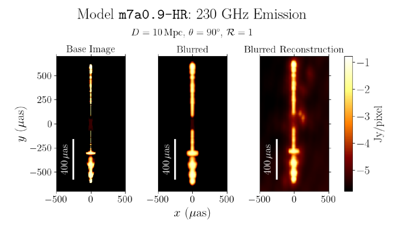
Figure 2: Model m7a0.9-HR at $t=78,000\,t_{g}$ imaged at $D=10$ Mpc with $\theta=90^{\circ}$ and $\mathcal{R}=1$. We show the base ipole image with no blurring (left), the base ipole image blurred via convolution with a $20\,\mu\rm{as}$ FWHM Gaussian beam (middle), and the reconstructed image blurred using the same Gaussian beam (right).

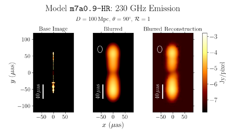
Figure 3: The same as Figure 2 but for model m7a0.9-HR at $t=78,000\,t_{g}$ imaged at $D=100$ Mpc with $\theta=90^{\circ}$ and $\mathcal{R}=1$.

3.2 Tracking Jet Motion

In this subsection, we demonstrate that the original ray traced images and the reconstructed images allow for the jet motion to be tracked and yield similar results for the time evolution of the jet. The jet features are approximately Lorentzian, so we fit Lorentzian profiles to the image to find the position of the top and bottom jet in both the base images and the reconstructed images. We detail the peak finding algorithm in Appendix B. Since we cannot properly center the jet in the reconstructed images (there is no bright, central radiation from the near BH), we only measure the distance between the two jet peaks $y_{1}$ and $y_{2}$, respectively. We define the apparent jet length as:

$$l_{\rm{jet}}=|y_{2}-y_{1}|.$$ (9)

Note that we have not differentiated the ’top’ or ’bottom’ jet here as we are only concerned with the total distance between the jet heads. We obtain errors on the jet length from the error estimates of the jet head locations using standard error propagation analysis:

$$\delta l_{\rm{jet}}=\sqrt{\delta y_{1}^{2}+\delta y_{2}^{2}}.$$ (10)

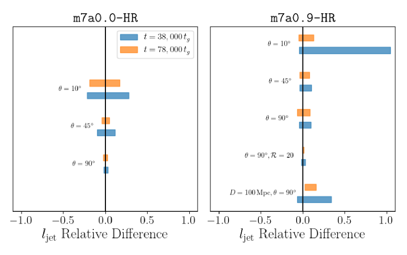
Figure 4: Here we show the relative difference at the 3 standard deviation level (colored horizontal bars) between the jet lengths obtained from the ray traced images $(l_{\rm{jet}})$ and the reconstructed images $(l_{\rm{jet,rec}})$. Models m7a0.0-HR (left panel) and m7a0.9-HR (right panel) are shown. For each choice of viewing angle $\theta$, distance to the source $D$, and $\mathcal{R}$, we show the data at $t=38,000\,t_{g}$ (blue) and $t=78,000\,r_{g}$. We indicate the viewing angle next to each pairing of error bars. For each model, except where explicitly indicated to be otherwise, we show $D=10$ Mpc and $\mathcal{R}=1$. The figure is described in the text.

We compute the relative difference between the jet lengths for the ray traced ($l_{\rm{jet}}$) and reconstructed ($l_{\rm{jet,rec}}$) images in order to quantify the extent to which measurements of the jet length and velocity agree. We find that, generally, the ray traced and reconstructed images yield similar jet lengths within $3\delta l_{\rm{jet}}$ (Figure 3). In general, there are much larger errors on the fit for the Lorentzian profile’s center at steep angles (i.e. see the relative difference for $\theta=10^{\circ}$). The agreement is also effected by how bright the source is, as illustrated by the shift to the right for model m7a0.9-HR when $D=100$ Mpc. We compile estimates of the jet lengths for each image in Table 3.

Since we lack centering information in the reconstructed images, we choose to estimate the jet velocity perpendicular to the line of sight by assuming both the top and bottom jet have the same speed. Then the velocity of the centroids of the jet in the source’s frame are:

$$v_{\rm{cen}}=\dfrac{1}{2}\dfrac{|l_{\rm{jet}}(t_{2})-l_{\rm{jet}}(t_{1})|}{t_{2}-t_{1}}.$$ (11)

Note that we use the same expression to derive the centroid velocity in the reconstructed images ($v_{\rm{cen,rec}}$) but replace $l_{\rm{jet}}$ with $l_{\rm{jet,rec}}$ in Equation 11. Very Long Baseline Interferometry (VLBI) observations will provide the apparent motion of the jet, which may be superluminal due to relativistic effects. To account for this, we assume each centroid has a velocity of $v_{\rm{cen,rec}}$ and then estimate the apparent velocity ($v_{\rm{app,rec}}$) via the time in the observer’s frame ($t_{1}^{\prime}$,$t_{2}^{\prime}$):

$$v_{\rm{app,rec}}=\dfrac{1}{2}\dfrac{|l_{\rm{jet,rec}}(t_{2}^{\prime})-l_{\rm{jet,rec}}(t_{1}^{\prime})|}{t_{2}^{\prime}-t_{1}^{\prime}}=v_{\rm{cen,rec}}\left(1-\dfrac{v_{\rm{cen,rec}}}{c}\dfrac{\cos\theta}{\sin\theta}\right)^{-1}.$$ (12)

Here we have used the relationship

$$t_{2}^{\prime}-t_{1}^{\prime}=(t_{2}-t_{1})\left(1-\dfrac{v_{\rm{cen,rec}}}{c}\dfrac{\cos\theta}{\sin\theta}\right)$$ (13)

in the last expression. Note that the division by $\sin\theta$ is to account for the fact the $v_{\rm{cen,rec}}$ measures the velocity parallel to the line of sight with no time delay effects while we require an estimate of the velocity along the jet axis (which we can obtain since the geometry is fully known). We only present the apparent velocity for the reconstructed images ($v_{\rm{app,rec}}$) since this represents an estimate of what VLBI observations would truly see.

We use the data at $t_{1}=38,000\,t_{g}$ and $t_{2}=78,000\,t_{g}$ for each model to estimate the jet velocity. We tabulate the estimated centroid velocity and apparent velocity for each model in Table 4. We find excellent agreement between the velocities derived from the ray traced and reconstructed images. It is interesting to note the apparently faster jet for $\mathcal{R}=20$. We suspect the increased speed is due to the emitting material being dominated by material near the jet axis rather than some of the slower moving material around the jet head, which does not produce much emission at 230 GHz as the electron temperature is reduced. The more powerful jet model m7a0.9-HR demonstrates that such jets may appear as superluminal sources as we find a maximum $v_{\rm{app,rec}}\approx 1.526c$ at $\theta=10^{\circ}$.

Table 3: Here we tabulate the estimated jet length for each model at each time for different choices of the distance $D$, viewing angle $\theta$, and plasma temperature ratio $\mathcal{R}$. We compare the jet length as computed from the base ipole image ($l_{\rm{jet}}$) and the reconstructed image ($l_{\rm{jet,rec}}$).

Model	Time	Distance	$\theta$	$\mathcal{R}$	$l_{\rm{jet}}$	$l_{\rm{jet,rec}}$
	$(t_{g})$	(Mpc)			$(r_{g})$	$(r_{g})$
m7a0.0-HR	$38,000$	$10$	$10^{\circ}$	1	$5091^{+272}_{-272}$	$4927^{+317}_{-317}$
	$78,000$	$10$	$10^{\circ}$	1	$9042^{+356}_{-356}$	$9104^{+407}_{-407}$
	$38,000$	$10$	$45^{\circ}$	1	$22,006^{+123}_{-123}$	$21,774^{+731}_{-731}$
	$78,000$	$10$	$45^{\circ}$	1	$39,832^{+318}_{-318}$	$39,678^{+501}_{-501}$
	$38,000$	$10$	$90^{\circ}$	1	$28,658^{+148}$	$28,463^{+173}_{-173}$
	$78,000$	$10$	$90^{\circ}$	1	$57,068^{+401}_{-401}$	$56,844^{+237}_{-237}$
m7a0.9-HR	$38,000$	$10$	$10^{\circ}$	1	$8457^{+446}_{-446}$	$4191^{+726}_{-726}$
	$78,000$	$10$	$10^{\circ}$	1	$17,585^{+233}_{-233}$	$16,837^{+726}_{-726}$
	$38,000$	$10$	$45^{\circ}$	1	$33,128^{+336}_{-336}$	$31,941^{+683}_{-683}$
	$78,000$	$10$	$45^{\circ}$	1	$73,535^{+890}_{-890}$	$71,855^{+1058}_{-1058}$
	$38,000$	$10$	$90^{\circ}$	1	$48,468^{+306}_{-306}$	$46,972^{+1028}_{-1028}$
	$78,000$	$10$	$90^{\circ}$	1	$111,503^{+1085}_{-1085}$	$110,327^{+2657}_{-2657}$
	$38,000$	$10$	$90^{\circ}$	20	$49,457^{+150}_{-150}$	$48,930^{+358}_{-358}$
	$78,000$	$10$	$90^{\circ}$	20	$119,897^{+173}_{-173}$	$119,256^{+415}_{-415}$
	$38,000$	$100$	$90^{\circ}$	1	$46,715^{+400}_{-400}$	$40,244^{+2714}_{-2714}$
	$78,000$	$100$	$90^{\circ}$	1	$109,091^{+959}_{-959}$	$98,822^{+2075}_{-2075}$

Table 4: Here we tabulate the estimated jet velocity for each model for different choices of the distance $D$, viewing angle $\theta$, and plasma temperature ratio $\mathcal{R}$. The velocities shown are calculated using the base ipole images ($v_{\rm{cen}}$), the reconstructed images ($v_{\rm{cen,rec}}$), and the reonstructed images and accounting for the possibility of superluminal motion ($v_{\rm{app,rec}}$).

Model	Distance	$\theta$	$\mathcal{R}$	$v_{\rm{cen}}$	$v_{\rm{cen,rec}}$	$v_{\rm{app,rec}}$
	(Mpc)			$(c)$	$(c)$	$(c)$
m7a0.0-HR	$10$	$10^{\circ}$	1	$0.049^{+0.006}_{-0.006}$	$0.052^{+0.006}_{-0.006}$	$0.074^{+0.009}_{-0.009}$
	$10$	$45^{\circ}$	1	$0.223^{+0.005}_{-0.005}$	$0.224^{+0.011}_{-0.011}$	$0.288^{+0.014}_{-0.014}$
	$10$	$90^{\circ}$	1	$0.355^{+0.005}_{-0.005}$	$0.355^{+0.004}_{-0.004}$	$0.355^{+0.004}_{-0.004}$
m7a0.9-HR	$10$	$10^{\circ}$	1	$0.114^{+0.006}_{-0.006}$	$0.158^{+0.011}_{-0.011}$	$1.526^{+0.102}_{-0.102}$
	$10$	$45^{\circ}$	1	$0.505^{+0.012}_{-0.012}$	$0.499^{+0.016}_{-0.016}$	$0.996^{+0.031}_{-0.031}$
	$10$	$90^{\circ}$	1	$0.788^{+0.014}_{-0.014}$	$0.792^{+0.036}_{-0.036}$	$0.792^{+0.036}_{-0.036}$
	$10$	$90^{\circ}$	20	$0.88^{+0.002}_{-0.002}$	$0.879^{+0.007}_{-0.007}$	$0.879^{+0.007}_{-0.007}$
	$100$	$90^{\circ}$	1	$0.780^{0.013}_{-0.013}$	$0.732^{+0.043}_{-0.043}$	$0.732^{+0.043}_{-0.043}$

4 Discussion

4.1 Extracting Jet Physics from VLBI Images

A key feature of the jets in our models is the bright “bubbles” (or knots) of 230 GHz emission, which appear to correlate with recollimation shocks. Such structures have been seen in VLBI images of various AGN jets Jorstad et al. (2005); Lister et al. (2013); Cohen et al. (2014). Previous simulations of jets in various astrophysical contexts have demonstrated that recollimation occurs when there is a pressure mismatch between the jet and the surrounding medium, which could be a static atmosphere or a slower moving jet sheath Kohler et al. (2012); Lazzati et al. (2012); Mizuno et al. (2015); Hervet et al. (2017). The number of recollimation shocks along the jet axis are dependent on the properties of the jet and medium. It is therefore possible that direct VLBI of TDE jets will allow in depth modeling of jet launching and could also aid in constraining the properties of the surrounding medium. For instance, one work successfully applied simulations of MHD jets to constrain properties of BL Lacartae, which is a blazar jet with recollimation features Gómez et al. (2016).

We suggest that a similar approach may be applied in TDE jets. With a suitable exploration of the parameter space, it is conceivable that an analysis similar to that of Gómez et al. (2016) could be applied to TDE jets in cases where VLBI is possible. A broader exploration of TDE jets through various simulation methodologies is strongly suggested. We plan to explore the effects of the ambient medium, magnetic field strength, and disk accretion rate on the jet properties in the case of a SANE, super-Eddington disk in a future work.

4.2 Proposed Observational Methodology

Our synthetic ngEHT observations demonstrate that a 24-hour observation may be sufficient to study both the structure and/or motion of newly born TDE jets. This is much shorter than the fallback time, which is on the order of month(s), as well as the duration of radio emission in several TDEs, which can sometimes be visible for years Alexander et al. (2020). Our suggested observational strategy is conducting rapid followup of newly discovered optical/X-ray TDEs when they are near the peak of their emission in order to study both the early- and late-time properties of their jets (if present). Observations with a single telescope at 230 GHz can be conducted to search for TDEs emitting in the radio. If emission at 230 GHz is detected, we suggest that the ngEHT conduct VLBI follow-up of targets within no more than a month. Our imaging simulations were done assuming a full ngEHT array consisting of the 2022 EHT stations plus 11 additional sites, but depending on the target not all sites may need to be available in order to obtain a high-fidelity image reconstruction.

Unlike many other EHT/ngEHT targets, TDEs will appear randomly across the sky and the ngEHT will need to be capable of follow-up observations on the order of a week to weeks. Our current modeling of jets and outflows from super-Eddington disks is too sparse to make predictions regarding how long the jets will be visible at 230 GHz. However, if radio TDE observations are any indicator, emission may persist for many months Alexander et al. (2020).

TDEs provide an excellent laboratory for studying jet/accretion/black hole systems across a wide range of accretion states over a relatively short period of time ($\sim$1-a few years). In several cases, TDEs have shown state transitions after several hundred days in the X-ray which are likely associated with the evolution of the disk as the mass accretion rate declines. Stone and Metzger (2016) argue for instance that the transition from a thick, super-Eddington disk to a thin disk can explain the jet shut-off in jetted TDEs such as Swift J1644+57 and Swift J2058+05 Zauderer et al. (2013); Pasham et al. (2015), but recent simulations Curd and Narayan (2022); Liska et al. (2022) demonstrate that MAD is possible even for thinner accretion disks. As such, long term VLBI monitoring is strongly suggested as this would allow for (1) the radio-submm emission of the outflows to be characterized and compared to the behaviour of the accretion flow, and (2) the direct study of how the jet evolves morphologically as the disk state changes.

Another attractive potential target which we have yet to attribute a self-contained study to is jetted TDEs. These TDEs are extremely rare and current observations suggest only about 1% of all TDEs will produce powerful relativistic jets. These jets will produce extremely bright radiation in the X-ray as well as the radio-submm. However, most have been distant due to the lower probability of their occurrence. Should a jetted TDE occur nearby enough for VLBI to resolve the jet, we strongly suggest such jets be treated as targets of opportunity for the ngEHT.

Lastly, a recent TDE AT2018hyz showed a late outflow ($\sim 3$ years after the initial outburst) and brightened in the radio over several hundred days Cendes et al. (2022). Unlike many other radio TDEs, relatively bright 240 GHz emission was detected. If AT2018hyz is in fact a jet instead of a spherical outflow, Cendes et al. (2022) estimate that the velocity could reach $\lesssim 0.6c$. AT2018hyz is a relatively nearby TDE at $\sim 204$ Mpc, but the flux density at the time of detection ($\sim 0.2$ mJy at 240 GHz) makes it too dim for ngEHT follow-up. However, placing AT2018hyz at $\sim 50$ Mpc would shift the flux density to $\sim 5$ mJy, which is the minimum estimated flux density required for an ngEHT VLBI detection. Future TDEs will likely be monitored across the radio-submm, so nearby targets of opportunity such as late radio TDEs like AT2018hyz should be considered should they show significant radio emission.

5 Conclusions

In this work, we have demonstrated through a synthetic imaging analysis that TDE jets resembling the GRRMHD models presented in Curd et al. (2022) are compelling ngEHT targets. We also confirm that the detection limits considered in Curd et al. (2022) are roughly applicable as m7a0.0-HR did not produce detectable emission at a distance of 100 Mpc in our imaging analysis.

Various shock features in the jet are visible for the $10$ Mpc images we consider, and studying the jet morphology in these cases could aid in characterizing the environment of the BH. Most TDEs that occur during the ngEHT mission will be farther away, but the apparent motion, which may be superluminal, can be extracted in such cases.

We suggest that the ngEHT be utilized for radio follow-up of TDEs. Our models study the birth of a TDE jet in the first $\sim 48$ days after the disk forms under the assumption that the disk is SANE, super-Eddington, and threaded by a dynamically important magnetic field. However, TDEs which occur nearby and have jet properties similar to jetted TDEs such as Swift J1644+57 or AT2018hyz may provide interesting targets of opportunity.

Brandon Curd was supported by NSF grant AST-1816420, and made use of computational support from NSF via XSEDE/ACCESS resources (grant TG-AST080026N). Razieh Emami acknowledges the support by the Institute for Theory and Computation at the Center for Astrophysics as well as grant numbers 21-atp21-0077, NSF AST-1816420 and HST-GO-16173.001-A for very generous supports. Freek Roelofs was supported by NSF grants AST-1935980 and AST-2034306. This work was supported by the Black Hole Initiative at Harvard University, made possible through the support of grants from the Gordon and Betty Moore Foundation and the John Templeton Foundation. The opinions expressed in this publication are those of the author(s) and do not necessarily reflect the views of the Moore or Templeton Foundations.

Acknowledgements  We graciously acknowledge Koushik Chatterjee, Lani Oramas, Joaquin Duran, and Hayley West for fruitful discussions helpful in the preparation of this work. no

Appendix A Full Image Library

In Figures 5-8, we show the full library of images analyzed in this work. All of the base images were ray traced at $\nu=230$ GHz and then convolved with a Gaussian beam with a FWHM of 20 $\mu$as. Similarly, we blur the reconstructed image using the same beam for comparison. Note that in Figures 6 and 8, we have also shifted the reconstructed image to be approximately centered for comparison with the base image. In general, bright features are represented quite well in the reconstruction; however, some noise is introduced in dimmer sources (i.e. see the reconstruction of m7a0.9-HR at $D=100$ Mpc).

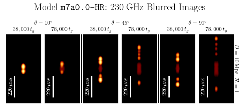
Figure 5: Here we show the full library of base ipole images for model m7a0.0-HR. The time of each column is indicated at the top while the distance $D$ and plasma temperature ratio $\mathcal{R}$ for each row are indicated on the right. The angle of the observer relative to the jet axis is indicated above each set of two rows. Each image spans $550\times 770\,\mu\rm{as}^{2}$ and is blurred by convolving the base image with a Gaussian beam with a FWHM of $20\,\mu\rm{as}$. The colour scale is logarithmic, spanning three orders of magnitude, and each image uses the same maximum for the intensity scale.

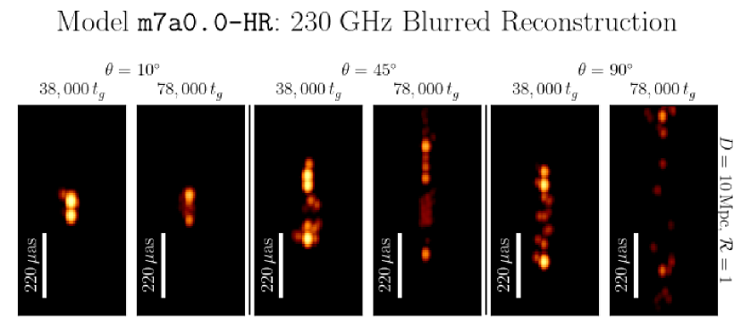
Figure 6: The same as Figure 5 but showing the reconstructed images. Note that the intensity scale for each panel is the same as the corresponding panel in Figure 5 for comparison.

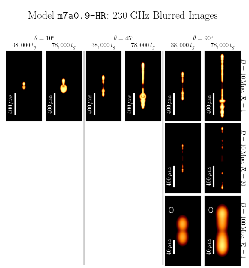
Figure 7: Here we show the full library of base ipole images for model m7a0.9-HR. Each image in the top and middle rows spans $1000\times 1400\,\mu\rm{as}^{2}$ while the bottom row spans $170\times 238\,\mu\rm{as}^{2}$. Each image is blurred by convolving the base image with a Gaussian beam with a FWHM of $20\,\mu\rm{as}$ (indicated by the white circle in the bottom right panel). The time of each column is indicated at the top while the distance $D$ and plasma temperature ratio $\mathcal{R}$ for each row are indicated on the right. The angle of the observer relative to the jet axis is indicated above each set of two rows. The colour scale is logarithmic, spanning three orders of magnitude in each image. We use the same colour scale for the $D=10$ Mpc images, but reduce the maximum by an order of magnitude in the $D=100$ Mpc images to better show the image features.

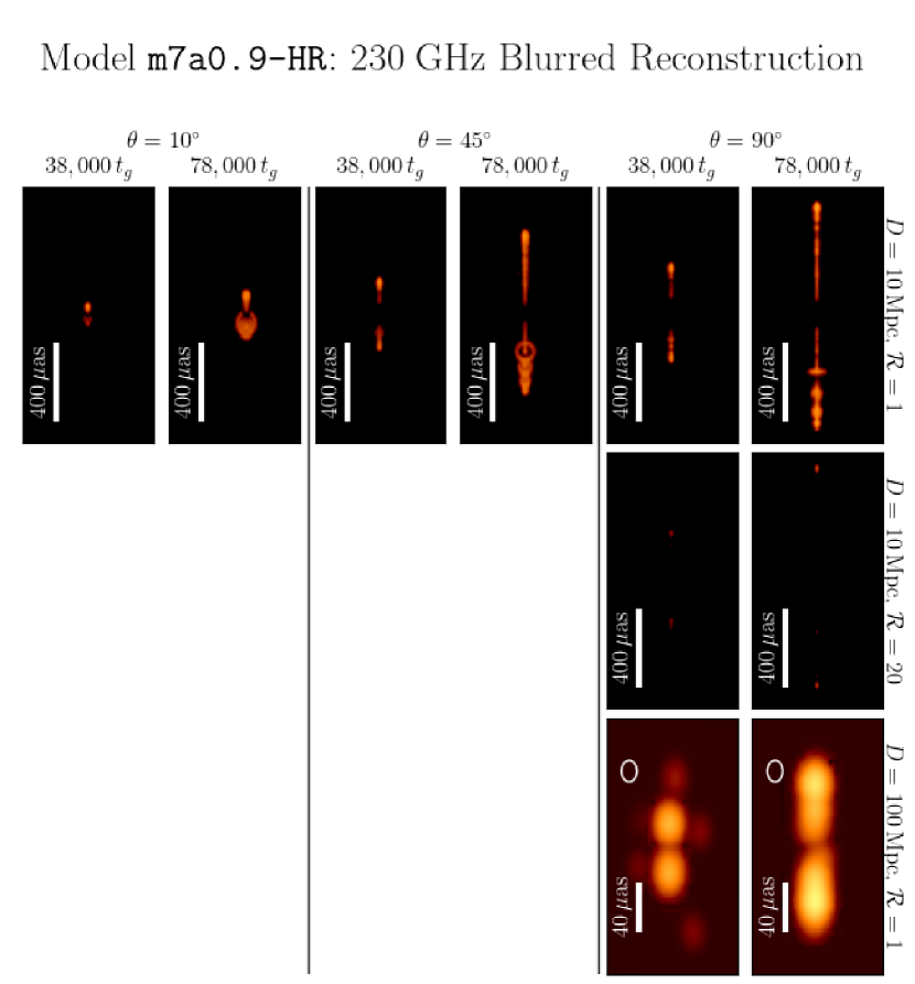
Figure 8: The same as Figure 7 but showing the reconstructed images. Note that the intensity scale for each panel is the same as the corresponding panel in Figure 7 for comparison.

Appendix B Fitting Procedure for Jet Head Position

Here we describe the algorithm implemented to estimate the position of the top and bottom jet heads in each image. In order to track the jet’s motion, we first smooth the data (either the base image or the reconstructed image) with a Gaussian beam which assumes an angular resolution for the VLBI observations of $\Delta\theta=20\mu{\rm{as}}$. We then bin the data along the symmetry axis of the jet ($y$) by summing the flux along each row ($x$).

Since the images appear to be roughly Lorentzian, we first attempt to fit a double Lorentzian function of the form:

$$f_{d}(y)=a_{1}\dfrac{w_{1}^{2}}{(y-y_{{\rm{cen}},2})^{2}+w_{1}^{2}}+a_{2}\dfrac{w_{2}^{2}}{(y-y_{{\rm{cen}},2})^{2}+w_{2}^{2}},$$ (14)

where $a$ is the amplitude, $w$ is the width, and $y_{\rm{cen}}$ is the center defining the curve. We take $y_{\rm{cen}}$ as a measure of the jet head location. If this fitting procedure does not produce a good fit, we find the peaks by performing a two-step fitting procedure in which we fit a single Lorentzian:

$$f_{1}(y)=a_{1}\dfrac{w_{1}^{2}}{{(y-y_{{\rm{cen}},1}})^{2}+w_{1}^{2}},$$ (15)

and then subtract the fit $f_{1}(y)$ from the data and then fit the second peak with:

$$f_{2}(y)=a_{2}\dfrac{w_{2}^{2}}{{(y-y_{{\rm{cen}},2}})^{2}+w_{2}^{2}}.$$ (16)

We implement the python package, SciPy Virtanen et al. (2020), to optimize the curve(s) and estimate the jet head positions and errors. We show an example of the data and the Lorentzian fit for both the base image and the Reconstruction in Figure 9. The reconstruction tends to be a bit broader, but the fitting procedure works equally well for all images and reconstructed images.

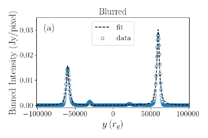
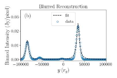
Figure 9: We demonstrate the fit performance using a ray traced image of model m7a0.9-HR at $t=78,000\,t_{g}$, $\theta=90^{\circ}$, $D=10$ Mpc, and $\mathcal{R}=20$. We show the $x$-binned data and a double Lorentzian (Equation 14) fit for (a) the blurred base image, and (b) the blurred reconstruction.

References

References

- Hills (1975) Hills, J.G. Possible power source of Seyfert galaxies and QSOs. Nature 1975, 254, 295–298. https://doi.org/10.1038/254295a0.
- Rees (1988) Rees, M.J. Tidal disruption of stars by black holes of 106-108 solar masses in nearby galaxies. Nature 1988, 333, 523–528. https://doi.org/10.1038/333523a0.
- Guillochon and Ramirez-Ruiz (2013) Guillochon, J.; Ramirez-Ruiz, E. Hydrodynamical Simulations to Determine the Feeding Rate of Black Holes by the Tidal Disruption of Stars: The Importance of the Impact Parameter and Stellar Structure. ApJ 2013, 767, 25, [arXiv:astro-ph.HE/1206.2350]. https://doi.org/10.1088/0004-637X/767/1/25.
- Mainetti et al. (2017) Mainetti, D.; Lupi, A.; Campana, S.; Colpi, M.; Coughlin, E.R.; Guillochon, J.; Ramirez-Ruiz, E. The fine line between total and partial tidal disruption events. A&A 2017, 600, A124, [arXiv:astro-ph.HE/1702.07730]. https://doi.org/10.1051/0004-6361/201630092.
- Steinberg and Stone (2022) Steinberg, E.; Stone, N.C. The Origins of Peak Light in Tidal Disruption Events, 2022. https://doi.org/10.48550/ARXIV.2206.10641.
- Stone et al. (2013) Stone, N.; Sari, R.; Loeb, A. Consequences of strong compression in tidal disruption events. MNRAS 2013, 435, 1809–1824, [arXiv:astro-ph.HE/1210.3374]. https://doi.org/10.1093/mnras/stt1270.
- Golightly et al. (2019) Golightly, E.C.A.; Nixon, C.J.; Coughlin, E.R. On the Diversity of Fallback Rates from Tidal Disruption Events with Accurate Stellar Structure. ApJ 2019, 882, L26, [arXiv:astro-ph.HE/1907.05895]. https://doi.org/10.3847/2041-8213/ab380d.
- Komossa (2015) Komossa, S. Tidal disruption of stars by supermassive black holes: Status of observations. Journal of High Energy Astrophysics 2015, 7, 148–157, [arXiv:astro-ph.HE/1505.01093]. https://doi.org/10.1016/j.jheap.2015.04.006.
- Gezari (2021) Gezari, S. Tidal Disruption Events. ARA&A 2021, 59, [arXiv:astro-ph.HE/2104.14580]. https://doi.org/10.1146/annurev-astro-111720-030029.
- Alexander et al. (2020) Alexander, K.D.; van Velzen, S.; Horesh, A.; Zauderer, B.A. Radio Properties of Tidal Disruption Events. Space Sci. Rev. 2020, 216, 81, [arXiv:astro-ph.HE/2006.01159]. https://doi.org/10.1007/s11214-020-00702-w.
- Dai et al. (2018) Dai, L.; McKinney, J.C.; Roth, N.; Ramirez-Ruiz, E.; Miller, M.C. A Unified Model for Tidal Disruption Events. ApJ 2018, 859, L20, [arXiv:astro-ph.HE/1803.03265]. https://doi.org/10.3847/2041-8213/aab429.
- Curd et al. (2022) Curd, B.; Emami, R.; Anantua, R.; Palumbo, D.; Doeleman, S.; Narayan, R. Jets from SANE Super-Eddington Accretion Disks: Morphology, Spectra, and Their Potential as Targets for ngEHT. arXiv e-prints 2022, p. arXiv:2206.06358, [arXiv:astro-ph.HE/2206.06358].
- Gammie et al. (2003) Gammie, C.F.; McKinney, J.C.; Tóth, G. HARM: A Numerical Scheme for General Relativistic Magnetohydrodynamics. ApJ 2003, 589, 444–457, [arXiv:astro-ph/astro-ph/0301509]. https://doi.org/10.1086/374594.
- Tchekhovskoy et al. (2014) Tchekhovskoy, A.; Metzger, B.D.; Giannios, D.; Kelley, L.Z. Swift J1644+57 gone MAD: the case for dynamically important magnetic flux threading the black hole in a jetted tidal disruption event. MNRAS 2014, 437, 2744–2760, [arXiv:astro-ph.HE/1301.1982]. https://doi.org/10.1093/mnras/stt2085.
- Curd and Narayan (2019) Curd, B.; Narayan, R. GRRMHD simulations of tidal disruption event accretion discs around supermassive black holes: jet formation, spectra, and detectability. MNRAS 2019, 483, 565–592, [arXiv:astro-ph.HE/1811.06971]. https://doi.org/10.1093/mnras/sty3134.
- Blandford and Znajek (1977) Blandford, R.D.; Znajek, R.L. Electromagnetic extraction of energy from Kerr black holes. MNRAS 1977, 179, 433–456. https://doi.org/10.1093/mnras/179.3.433.
- Coughlin and Begelman (2020) Coughlin, E.R.; Begelman, M.C. Structured, relativistic jets driven by radiation. MNRAS 2020, 499, 3158–3177, [arXiv:astro-ph.HE/2009.03898]. https://doi.org/10.1093/mnras/staa3026.
- Thomsen et al. (2022) Thomsen, L.L.; Kwan, T.M.; Dai, L.; Wu, S.C.; Roth, N.; Ramirez-Ruiz, E. Dynamical Unification of Tidal Disruption Events. ApJ 2022, 937, L28, [arXiv:astro-ph.HE/2206.02804]. https://doi.org/10.3847/2041-8213/ac911f.
- Doeleman et al. (2019) Doeleman, S.; Blackburn, L.; Dexter, J.; Gomez, J.L.; Johnson, M.D.; Palumbo, D.C.; Weintroub, J.; Farah, J.R.; Fish, V.; Loinard, L.; et al. Studying Black Holes on Horizon Scales with VLBI Ground Arrays. In Proceedings of the Bulletin of the American Astronomical Society, 2019, Vol. 51, p. 256, [arXiv:astro-ph.IM/1909.01411].
- Ivezić et al. (2019) Ivezić, Ž.; Kahn, S.M.; Tyson, J.A.; Abel, B.; Acosta, E.; Allsman, R.; Alonso, D.; AlSayyad, Y.; Anderson, S.F.; Andrew, J.; et al. LSST: From Science Drivers to Reference Design and Anticipated Data Products. ApJ 2019, 873, 111, [arXiv:astro-ph/0805.2366]. https://doi.org/10.3847/1538-4357/ab042c.
- Bricman and Gomboc (2020) Bricman, K.; Gomboc, A. The Prospects of Observing Tidal Disruption Events with the Large Synoptic Survey Telescope. ApJ 2020, 890, 73, [arXiv:astro-ph.HE/1906.08235]. https://doi.org/10.3847/1538-4357/ab6989.
- Stone and Metzger (2016) Stone, N.C.; Metzger, B.D. Rates of stellar tidal disruption as probes of the supermassive black hole mass function. MNRAS 2016, 455, 859–883, [arXiv:astro-ph.HE/1410.7772]. https://doi.org/10.1093/mnras/stv2281.
- Sadowski et al. (2016) Sadowski, A.; Tejeda, E.; Gafton, E.; Rosswog, S.; Abarca, D. Magnetohydrodynamical simulations of a deep tidal disruption in general relativity. Mon. Not. Roy. Astron. Soc. 2016, 458, 4250–4268, [arXiv:astro-ph.HE/1512.04865]. https://doi.org/10.1093/mnras/stw589.
- Curd (2021) Curd, B. Global simulations of tidal disruption event disc formation via stream injection in GRRMHD. Mon. Not. Roy. Astron. Soc. 2021, 507, 3207–3227, [arXiv:astro-ph.HE/2105.09904]. https://doi.org/10.1093/mnras/stab2172.
- Novikov and Thorne (1973) Novikov, I.D.; Thorne, K.S. Astrophysics of black holes. In Proceedings of the Black Holes (Les Astres Occlus), 1973, pp. 343–450.
- Mościbrodzka and Gammie (2018) Mościbrodzka, M.; Gammie, C.F. IPOLE - semi-analytic scheme for relativistic polarized radiative transport. MNRAS 2018, 475, 43–54, [arXiv:astro-ph.HE/1712.03057]. https://doi.org/10.1093/mnras/stx3162.
- Yarza et al. (2020) Yarza, R.; Wong, G.N.; Ryan, B.R.; Gammie, C.F. Bremsstrahlung in GRMHD Models of Accreting Black Holes. ApJ 2020, 898, 50, [arXiv:astro-ph.HE/2006.01145]. https://doi.org/10.3847/1538-4357/ab9808.
- Wong et al. (2022) Wong, G.N.; Prather, B.S.; Dhruv, V.; Ryan, B.R.; Mościbrodzka, M.; Chan, C.k.; Joshi, A.V.; Yarza, R.; Ricarte, A.; Shiokawa, H.; et al. PATOKA: Simulating Electromagnetic Observables of Black Hole Accretion. ApJS 2022, 259, 64, [arXiv:astro-ph.HE/2202.11721]. https://doi.org/10.3847/1538-4365/ac582e.
- Ohmura et al. (2019) Ohmura, T.; Machida, M.; Nakamura, K.; Kudoh, Y.; Asahina, Y.; Matsumoto, R. Two-Temperature Magnetohydrodynamics Simulations of Propagation of Semi-Relativistic Jets. Galaxies 2019, 7, 14. https://doi.org/10.3390/galaxies7010014.
- Ohmura et al. (2020) Ohmura, T.; Machida, M.; Nakamura, K.; Kudoh, Y.; Matsumoto, R. Two-temperature magnetohydrodynamic simulations for sub-relativistic active galactic nucleus jets: dependence on the fraction of the electron heating. MNRAS 2020, 493, 5761–5772, [arXiv:astro-ph.HE/2003.00795]. https://doi.org/10.1093/mnras/staa632.
- Raymond et al. (2021) Raymond, A.W.; Palumbo, D.; Paine, S.N.; Blackburn, L.; Córdova Rosado, R.; Doeleman, S.S.; Farah, J.R.; Johnson, M.D.; Roelofs, F.; Tilanus, R.P.J.; et al. Evaluation of New Submillimeter VLBI Sites for the Event Horizon Telescope. ApJS 2021, 253, 5, [arXiv:astro-ph.IM/2102.05482]. https://doi.org/10.3847/1538-3881/abc3c3.
- Roelofs et al. (2022, in prep.) Roelofs, F.; et al., 2022, in prep.
- Chael et al. (2016) Chael, A.A.; Johnson, M.D.; Narayan, R.; Doeleman, S.S.; Wardle, J.F.C.; Bouman, K.L. High-resolution Linear Polarimetric Imaging for the Event Horizon Telescope. ApJ 2016, 829, 11, [arXiv:astro-ph.IM/1605.06156]. https://doi.org/10.3847/0004-637X/829/1/11.
- Chael et al. (2018) Chael, A.A.; Johnson, M.D.; Bouman, K.L.; Blackburn, L.L.; Akiyama, K.; Narayan, R. Interferometric Imaging Directly with Closure Phases and Closure Amplitudes. ApJ 2018, 857, 23, [arXiv:astro-ph.IM/1803.07088]. https://doi.org/10.3847/1538-4357/aab6a8.
- Doeleman et al. (2022, in prep.) Doeleman, S.; et al., 2022, in prep.
- Gelaro et al. (2017) Gelaro, R.; McCarty, W.; Suárez, M.J.; Todling, R.; Molod, A.; Takacs, L.; Randles, C.A.; Darmenov, A.; Bosilovich, M.G.; Reichle, R.; et al. The Modern-Era Retrospective Analysis for Research and Applications, Version 2 (MERRA-2). Journal of Climate 2017, 30, 5419–5454, [https://journals.ametsoc.org/jcli/article-pdf/30/14/5419/4676847/jcli-d-16-0758_1.pdf]. https://doi.org/10.1175/JCLI-D-16-0758.1.
- Paine (2019) Paine, S. The am atmospheric model, 2019. https://doi.org/10.5281/zenodo.3406496.
- Event Horizon Telescope Collaboration et al. (2019) Event Horizon Telescope Collaboration.; Akiyama, K.; Alberdi, A.; Alef, W.; Asada, K.; Azulay, R.; Baczko, A.K.; Ball, D.; Baloković, M.; Barrett, J.; et al. First M87 Event Horizon Telescope Results. IV. Imaging the Central Supermassive Black Hole. ApJ 2019, 875, L4, [arXiv:astro-ph.GA/1906.11241]. https://doi.org/10.3847/2041-8213/ab0e85.
- Jorstad et al. (2005) Jorstad, S.G.; Marscher, A.P.; Lister, M.L.; Stirling, A.M.; Cawthorne, T.V.; Gear, W.K.; Gómez, J.L.; Stevens, J.A.; Smith, P.S.; Forster, J.R.; et al. Polarimetric Observations of 15 Active Galactic Nuclei at High Frequencies: Jet Kinematics from Bimonthly Monitoring with the Very Long Baseline Array. AJ 2005, 130, 1418–1465, [arXiv:astro-ph/astro-ph/0502501]. https://doi.org/10.1086/444593.
- Lister et al. (2013) Lister, M.L.; Aller, M.F.; Aller, H.D.; Homan, D.C.; Kellermann, K.I.; Kovalev, Y.Y.; Pushkarev, A.B.; Richards, J.L.; Ros, E.; Savolainen, T. MOJAVE. X. Parsec-scale Jet Orientation Variations and Superluminal Motion in Active Galactic Nuclei. AJ 2013, 146, 120, [arXiv:astro-ph.CO/1308.2713]. https://doi.org/10.1088/0004-6256/146/5/120.
- Cohen et al. (2014) Cohen, M.H.; Meier, D.L.; Arshakian, T.G.; Homan, D.C.; Hovatta, T.; Kovalev, Y.Y.; Lister, M.L.; Pushkarev, A.B.; Richards, J.L.; Savolainen, T. Studies of the Jet in Bl Lacertae. I. Recollimation Shock and Moving Emission Features. ApJ 2014, 787, 151, [arXiv:astro-ph.HE/1404.0976]. https://doi.org/10.1088/0004-637X/787/2/151.
- Kohler et al. (2012) Kohler, S.; Begelman, M.C.; Beckwith, K. Recollimation boundary layers in relativistic jets. MNRAS 2012, 422, 2282–2290, [arXiv:astro-ph.HE/1112.4843]. https://doi.org/10.1111/j.1365-2966.2012.20776.x.
- Lazzati et al. (2012) Lazzati, D.; Morsony, B.J.; Blackwell, C.H.; Begelman, M.C. Unifying the Zoo of Jet-driven Stellar Explosions. ApJ 2012, 750, 68, [arXiv:astro-ph.HE/1111.0970]. https://doi.org/10.1088/0004-637X/750/1/68.
- Mizuno et al. (2015) Mizuno, Y.; Gómez, J.L.; Nishikawa, K.I.; Meli, A.; Hardee, P.E.; Rezzolla, L. Recollimation Shocks in Magnetized Relativistic Jets. ApJ 2015, 809, 38, [arXiv:astro-ph.HE/1505.00933]. https://doi.org/10.1088/0004-637X/809/1/38.
- Hervet et al. (2017) Hervet, O.; Meliani, Z.; Zech, A.; Boisson, C.; Cayatte, V.; Sauty, C.; Sol, H. Shocks in relativistic transverse stratified jets. A new paradigm for radio-loud AGN. A&A 2017, 606, A103, [arXiv:astro-ph.HE/1705.10556]. https://doi.org/10.1051/0004-6361/201730745.
- Gómez et al. (2016) Gómez, J.L.; Lobanov, A.P.; Bruni, G.; Kovalev, Y.Y.; Marscher, A.P.; Jorstad, S.G.; Mizuno, Y.; Bach, U.; Sokolovsky, K.V.; Anderson, J.M.; et al. Probing the Innermost Regions of AGN Jets and Their Magnetic Fields with RadioAstron. I. Imaging BL Lacertae at 21 Microarcsecond Resolution. ApJ 2016, 817, 96, [arXiv:astro-ph.HE/1512.04690]. https://doi.org/10.3847/0004-637X/817/2/96.
- Zauderer et al. (2013) Zauderer, B.A.; Berger, E.; Margutti, R.; Pooley, G.G.; Sari, R.; Soderberg, A.M.; Brunthaler, A.; Bietenholz, M.F. Radio Monitoring of the Tidal Disruption Event Swift J164449.3+573451. II. The Relativistic Jet Shuts Off and a Transition to Forward Shock X-Ray/Radio Emission. ApJ 2013, 767, 152, [arXiv:astro-ph.HE/1212.1173]. https://doi.org/10.1088/0004-637X/767/2/152.
- Pasham et al. (2015) Pasham, D.R.; Cenko, S.B.; Levan, A.J.; Bower, G.C.; Horesh, A.; Brown, G.C.; Dolan, S.; Wiersema, K.; Filippenko, A.V.; Fruchter, A.S.; et al. A Multiwavelength Study of the Relativistic Tidal Disruption Candidate Swift J2058.4+0516 at Late Times. ApJ 2015, 805, 68, [arXiv:astro-ph.HE/1502.01345]. https://doi.org/10.1088/0004-637X/805/1/68.
- Curd and Narayan (2022) Curd, B.; Narayan, R. GRRMHD Simulations of MAD Accretion Disks Declining from Super-Eddington to Sub-Eddington Accretion Rates. arXiv e-prints 2022, p. arXiv:2209.12081, [arXiv:astro-ph.HE/2209.12081].
- Liska et al. (2022) Liska, M.T.P.; Musoke, G.; Tchekhovskoy, A.; Porth, O.; Beloborodov, A.M. Formation of Magnetically Truncated Accretion Disks in 3D Radiation-transport Two-temperature GRMHD Simulations. ApJ 2022, 935, L1, [arXiv:astro-ph.HE/2201.03526]. https://doi.org/10.3847/2041-8213/ac84db.
- Cendes et al. (2022) Cendes, Y.; Berger, E.; Alexander, K.D.; Gomez, S.; Hajela, A.; Chornock, R.; Laskar, T.; Margutti, R.; Metzger, B.; Bietenholz, M.F.; et al. A Mildly Relativistic Outflow Launched Two Years after Disruption in Tidal Disruption Event AT2018hyz. ApJ 2022, 938, 28, [arXiv:astro-ph.HE/2206.14297]. https://doi.org/10.3847/1538-4357/ac88d0.
- Virtanen et al. (2020) Virtanen, P.; Gommers, R.; Oliphant, T.E.; Haberland, M.; Reddy, T.; Cournapeau, D.; Burovski, E.; Peterson, P.; Weckesser, W.; Bright, J.; et al. SciPy 1.0: Fundamental Algorithms for Scientific Computing in Python. Nature Methods 2020, 17, 261–272. https://doi.org/10.1038/s41592-019-0686-2.