Abstract

We consider $Z^{\prime}$s in heterotic string derived models and study $Z^{\prime}$ resonant production at the TeV scale at the Large Hadron Collider (LHC). We use various kinematic differential distributions for the Drell-Yan process at NNLO in QCD to explore the parameter space of such models and investigate $Z^{\prime}$ couplings. In particular, we study the impact of $Z$-$Z^{\prime}$ kinetic-mixing interactions on forward-backward asymmetry ($A_{FB}$) and other distributions at the LHC.

1 Introduction

With the observation of a scalar particle compatible with the Standard Model electroweak Higgs doublet, the last piece in the Standard Model has been confirmed experimentally, and in the coming years its basic properties will be probed and elucidated. Furthermore, the discovery of the Higgs particle at 125 GeV suggests that the electroweak symmetry breaking mechanism is perturbative, rather than non-perturbative. This supports the old expectation that the Standard Model may provide viable parameterisation of particle physics data up to the Planck scale, where gravitational effects break the effective field theory description. Alas, the question remains how the Higgs mass and the ensuing electroweak symmetry breaking scales are protected from radiative corrections from the higher energy scale. While not yet seen at low energy experiments, supersymmetry remains one of the most appealing extensions of the Standard Model to address this puzzle. Furthermore, many supersymmetric models in fact predict that the Higgs particle should exist below 135 GeV. The observed Higgs particle is therefore compatible with supersymmetry. However, while supersymmetry protects the Higgs mass at the multi–loop level in the perturbative expansion, it introduces a problem at tree level, which is known as the $\mu$–problem. Supersymmetry mandates the existence of a pair of Higgs doublets, which can receive a bilinear mass term in the superpotential. In the Minimal Supersymmetric Standard Model, the $\mu$–parameter is therefore set by hand to be of the order of the electroweak scale, but nothing prevents it from being of the order of the Planck scale. Furthermore, absence of global symmetries in quantum gravity and the experience from quasi–realistic string derived models, do in fact suggest that generically the $\mu$–parameter will be of that order. A possible solution to the problem may be obtained if the Higgs states are chiral under an additional $U(1)$ symmetry, which remains unbroken down to TeV scale. In this case, the bi–linear mass term for the supersymmetric Higgs pair can only be generated by the vacuum Expectation Value (VEV) that breaks the extra $U(1)$ symmetry.

String theory provides the most developed framework to study the incorporation of the Standard Model in a perturbatively consistent theory of quantum gravity. Indeed, over the past few decades detailed phenomenological models have been built that produce the spectrum of the Minimal Supersymmetric Standard Model (MSSM) in the effective low energy field theory limit below the Planck scale (for review and references see e.g. [1]). The heterotic–string models constructed in the free fermionic formulation [2, 3, 4, 5], which are $Z_{2}\times Z_{2}$ orbifolds of six dimensional toroidal spaces [6], are among the most realistic models constructed to date, and give rise to an abundance of three generation models with different unbroken $SO(10)$ subgroups below the string scale. However, the construction of string models with additional $U(1)$ gauge symmetries, that may stay unbroken down to low scales, has proven to be a difficult task [7, 8]. The reason is that the extra $U(1)$ gauge symmetries that are often discussed in the context of Grand Unified Theory (GUT) extensions of the Standard Model are anomalous in explicit string models and therefore cannot remain unbroken down to low scales. In fact to date, there exist a single string derived model in which the extra $U(1)$ is anomaly free and can remain unbroken down to the TeV scale [9]. As a bonus the string derived model predicts the existence of electroweak doublet pairs at the $Z^{\prime}$ breaking scale, that are chiral under the extra $U(1)$ symmetry. The bilinear mass term for these electroweak Higgs doublets can therefore be generated only by the VEV that breaks the extra $U(1)$ symmetry.

In this paper, we therefore study some of the properties of the extra $U(1)$ symmetry predicted by the string model and explore the parameter space of the $Z^{\prime}$ by using various kinematic distributions of resonant lepton-pair production in the Drell-Yan (DY) process at the LHC. Other related literature can be found in refs. [10, 11, 12]. In addition, we study the effect of gauge kinetic-mixing interactions $\chi F^{\mu\nu}F^{\prime}_{\mu\nu}$ in the lagrangian [13]. The impact of such a renormalizable operator is interesting in this context because it may in general be produced (at both field theory or string theory level) by physics at high scales above the $Z^{\prime}$ breaking scale, with no suppression by the large-mass scale [14, 15] and can impact the couplings of $Z^{\prime}$s at the TeV scale [16]. The interplay between the gauge kinetic-mixing parameter and coupling of the $Z^{\prime}$, as well as other $Z^{\prime}$ properties, can be explored by using forward-backward asymmetry ($A_{FB}$) distributions in DY, where this observable can be advantageous in extra-resonance searches and as a model discrimination tool [17, 18, 19, 20, 21, 22, 23, 24, 25, 26, 27].

This paper is organized as follows. In Sec. 2 we describe the structure of the string derived $Z^{\prime}$ model. In Sec. 3 we discuss the phenomenological aspects of the model and analyze kinetic mixing. In Sec. 4 we illustrate and discuss our results. Finally, in Sec. 5 we present our conclusions.

2 The String Model 

We elaborate in this section on the structure of the string derived $Z^{\prime}$ model [9]. The model was constructed in the free fermionic formulation [28, 29, 30]. Only the important points relevant for the properties of the extra $Z^{\prime}$ gauge boson at low scales are discussed here and further details can be found in the original literature. Particularly relevant for the low energy phenomenology is the precise combination of worldsheet $U(1)$ currents predicted by the string model. In this respect we note that while similar aspects can be discussed in field theory models, in the string model the $U(1)$ combination is forced due to the available scalar multiplets to break the GUT symmetry, whereas in field theory models the scalar multiplets are a matter of choice.

In the free fermionic formulation all the worldsheet degrees of freedom required to cancel the conformal anomaly are represented in terms of free fermions propogating on the string worldsheet. In the standard notation the 64 worldsheet fermions in the lightcone gauge are denoted as:

${\underline{{\hbox{Left-Movers}}}}$:  $\psi^{\mu},~{}~{}{\chi_{i}},~{}~{}{y_{i},~{}~{}\omega_{i}}~{}~{}~{}~{}(\mu=1,2,~{}i=1,\cdots,6)$

${\underline{{\hbox{Right-Movers}}}}$

$${\bar{\phi}}_{A=1,\cdots,44}=\begin{cases}~{}~{}{{\bar{y}}_{i}~{},~{}{\bar{\omega}}_{i}}&i=1,{\cdots},6\cr&\cr~{}~{}{{\bar{\eta}}_{i}}&i=1,2,3{}{}\cr~{}~{}{{\bar{\psi}}_{1,\cdots,5}}&\cr~{}~{}{{\bar{\phi}}_{1,\cdots,8}}&\end{cases}$$

where the $\{y,\omega|{\bar{y}},{\bar{\omega}}\}^{1,\cdots,6}$ correspond to the six dimensions of the internally compactified manifold; ${\bar{\psi}}^{1,\cdots,5}$ generate the $SO(10)$ GUT symmetry; ${\bar{\phi}}^{1,\cdots,8}$ generate the hidden sector gauge group; and ${\bar{\eta}}^{1,2,3}$ generate three $U(1)$ gauge symmetries. Models in the free fermionic formulation are defined in terms of boundary condition basis vectors, which specify the transformation properties of the worldsheet fermions around the noncontractible loops of the vacuum to vacuum amplitude, and the Generalised GSO projection coefficients of the one loop partition function [28, 29, 30]. The free fermion models are $Z_{2}\times Z_{2}$ orbifold of six dimensional toroidal manifolds with discrete Wilson lines [6].

The Standard Model particle charges and data motivates the embedding of the Standard Model states in representations of Grand Unified Theories, like $SO(10)$ and $E_{6}$. The rank of these groups exceeds that of the Standard Model, and therefore they predict the existence of additional gauge symmetries, beyond the Standard Model. Compactifications of the heterotic–string to four dimensions do in fact give rise to $E_{6}$ GUT like models [31], which gives rise to string inspired $Z^{\prime}$ models. The additional $U(1)$ symmetries in these string inspired models have an $E_{6}$ embedding and produced numerous papers since the mid–eighties (for reviews and references see e.g. [32, 34, 19, 33, 10]). The construction of string derived models that allow for an unbroken extra $U(1)$ symmetry to remain unbroken down to low scales proves, however, to be very difficult. The symmetry breaking pattern $E_{6}\rightarrow SO(10)\times U(1)_{A}$ in the string derived models entails that $U(1)_{A}$ is anomalous and cannot be part of an unbroken $U(1)_{Z^{\prime}}$ at low energy scales [35]. String derived models with anomaly free $U(1)_{Z^{\prime}}\notin E_{6}$ were analysed in [36, 37, 38, 7], but agreement with the measured values of $\sin^{2}(\theta)_{W}(M_{Z})$ and $\alpha_{s}(M_{Z})$ favours $Z^{\prime}$ models with $E_{6}$ embedding [8]. We remark that the anomaly free $U(1)$ combination of $U(1)_{B-L}$ and $U(1)_{T_{3_{R}}}\in SO(10)$ may in principle stay unbroken down to low energy scales [39]. However, adequate suppression of the left–handed neutrino masses is facilitated if this $U(1)$ symmetry is broken at a high energy scale [40]. Constructing string models that enable an extra $U(1)\in E_{6}$ symmetry to stay unbroken down to low energy scales necessitates the construction of string models in which $U(1)_{A}$ is anomaly free. One method of achieving this outcome is to enhance $U(1)_{A}$ to a non-Abelian gauge symmetry á la ref. [41]. An alternative is the string derived model of ref. [9] that uses the Spinor–Vector Duality (SVD) that was observed in $Z_{2}\times Z_{2}$ orbifolds [42, 43, 44]. The SVD is under the exchange of the total number of $(16+\overline{16})$ representations of $SO(10)$ with the total number of $10$ representations, and is readily understood if we consider the enhancement of $SO(10)\times U(1)_{A}$ to $E_{6}$. The chiral and anti–chiral multiplets of $E_{6}$ decompose under $SO(10)\times U(1)$ as $27=16+10+1$ and $\overline{27}=\overline{16}+10+1$. In this case the $\#_{1}$ of $(16+\overline{16})$ and $\#_{2}$ of $10$ multiplets are equal. The $E_{6}$ symmetry point in the moduli space corresponds to a self–dual point under the exchange of the total number of $SO(10)$ spinorial plus anti–spinorial, with the total number of vectorial, multiplets. Breaking the $E_{6}$ gauge symmetry to $SO(10)\times U(1)_{A}$ results in the projection of some of the spinorial and vectorial multiplets, which results in $U(1)_{A}$ being anomalous. However, there may exist vacua with equal numbers of $(16+\overline{16})$ spinorial, and $10$ vectorial, multiplets, and traceless $U(1)_{A}$, without enhancement of the $SO(10)\times U(1)_{A}$ symmetry to $E_{6}$ [9]. In such models the chiral spectrum still forms complete $E_{6}$ representations, but the gauge symmetry is not enhanced to $E_{6}$. In this cases $U(1)_{A}$ is anomaly free and may remain unbroken down to low scales.

A fishing algorithm to extract models with specified physical properties was developed by using the free fermionic model building rules [45, 46, 47, 5, 48, 49, 50, 51]. In ref. [9], using the free fermionic fishing algorithm, such a spinor–vector self dual model was obtained with subsequent breaking at the string scale of the $SO(10)$ symmetry to the $SO(6)\times SO(4)$ subgroup, and preserves the spinor–vector self–duality. This model is a string derived model in which an extra $U(1)$ with $E_{6}$ embedding may remain unbroken down to low scales. The full massless spectrum of the string derived model is given in ref. [9]. The observable and hidden gauge groups at the string scale are produced by untwisted sector states and are given by:

$${\rm observable}~{}: ~{}~{}SO(6)\times SO(4)\times U(1)_{1}\times U(1)_{2}\times U(1)_{3}$$

$${\rm hidden}~{}: SO(4)^{2}\times SO(8)~{}~{}~{}~{}~{}~{}~{}~{}~{}~{}~{}~{}~{}~{}~{}~{}~{}~{}~{}~{}~{}~{}~{}~{}~{}~{}~{}~{}~{}~{}~{}$$

The massless string spectrum contains the fields required to break the GUT symmetry to the Standard Model.

The string model contains two anomalous $U(1)$ symmetries

$${\rm Tr}U(1)_{1}=36~{}~{}~{}~{}~{}~{}~{}{\rm and}~{}~{}~{}~{}~{}~{}~{}{\rm Tr}U(1)_{3}=-36.$$ (1)

The $E_{6}$ combination, given by,

$$U(1)_{\zeta}~{}=~{}U(1)_{1}+U(1)_{2}+U(1)_{3}~{},$$ (2)

is anomaly free and can be part of an unbroken $U(1)$ symmetry below the string scale. The $SO(6)\times SO(4)$ observable gauge symmetry is broken by the VEVs of the heavy Higgs fields ${\cal H}$ and $\overline{\cal H}$ . The charges of these fields under the Standard Model gauge group factors is given by:

$$\overline{\cal H}({\bf\bar{4}},{\bf 1},{\bf 2}) \rightarrow u^{c}_{H}\left({\bf\bar{3}},{\bf 1},\frac{2}{3}\right)+d^{c}_{H}\left({\bf\bar{3}},{\bf 1},-\frac{1}{3}\right)+$$

$$~{}~{}~{}~{}~{}~{}~{}~{}~{}~{}~{}~{}~{}~{}~{}~{}~{}~{}{\overline{\cal N}}\left({\bf 1},{\bf 1},0\right)+e^{c}_{H}\left({\bf 1},{\bf 1},-1\right)$$

$${\cal H}\left({\bf 4},{\bf 1},{\bf 2}\right) \rightarrow u_{H}\left({\bf 3},{\bf 1},-\frac{2}{3}\right)+d_{H}\left({\bf 3},{\bf 1},\frac{1}{3}\right)+$$

$$~{}~{}~{}~{}~{}~{}~{}~{}~{}~{}~{}~{}~{}~{}~{}~{}~{}~{}{\cal N}\left({\bf 1},{\bf 1},0\right)+e_{H}\left({\bf 1},{\bf 1},1\right)$$

The VEVs along the ${\cal N}$ and $\overline{\cal N}$ directions preserves $N=1$ spacetime supersymmetry along a flat direction and leave the $U(1)$ combination

$$U(1)_{{Z}^{\prime}}~{}=~{}\frac{1}{5}(U(1)_{C}-U(1)_{L})-U(1)_{\zeta}~{}\notin~{}SO(10),$$ (3)

unbroken below the string scale. This $U(1)$ combination is anomaly free provided that $U(1)_{\zeta}$ is anomaly free, as is the case in the string derived model [9].

We emphasise that this symmetry breaking pattern, and the $U(1)_{Z^{\prime}}$ combination in eq. (3) is enforced in the string derived model due the available scalar states in the string spectrum to break the non–Abelian $SO(6)\times SO(4)$ gauge symmetry, and due to a doublet–triplet missing partner mechanism [52] that gives heavy mass to coloured scalar states that arise in the untwisted sector of the string model [9]. Thus, the combination given in eq. (3) is the extra $U(1)$ combination that can arise in the string derived model with $E_{6}$ embedding of the charges. Contrary to the situation in string inspired model, where any combination of $U(1)_{C}-U(1)_{L}$ and $U(1)_{\zeta}$ is possible, the $U(1)$ combination $U(1)_{Z^{\prime}}$ is the uniquely predicted combination in the string derived model.

Anomaly cancellation of the $U(1)_{Z^{\prime}}$ gauge symmetry down to low scales, requires the vector–like leptons $\{H_{\textrm{vl}}^{i},{\bar{H}}_{\textrm{vl}}^{i}\}$, and quarks $\{D^{i},\overline{D}^{i}\}$, that are obtained from the vectorial $10$ multiplets of $SO(10)$, and the $SO(10)$ singlets $S^{i}$ in the $27$ representation of $E_{6}$. The supermultiplet states below the $SO(6)\times SO(4)$ breaking scale are displayed schematically in Table 1. The three right–handed neutrino $N_{L}^{i}$ states obtain heavy mass at the $SU(2)_{R}$ breaking scale, which produces the seesaw mechanism [53]. The spectrum below the $SU(2)_{R}$ breaking scale is assumed to be supersymmetric. We include in the spectrum an additional pair of vector–like electroweak Higgs doublets, that facilitate gauge coupling unification at the GUT scale. This is justified in the string inspired models due to the string doublet–triplet splitting mechanism [54, 55]. We note from table 1 that this extra Higgs pair is not chiral with respect to $U(1)_{Z^{\prime}}$, contrary to the three pairs, $\{H_{\textrm{vl}}^{i},{\bar{H}}_{\textrm{vl}}^{i}\}$, that are chiral with respect to $U(1)_{Z^{\prime}}$. Therefore, mass terms for these three pairs can only be generated by the breaking of $U(1)_{Z^{\prime}}$, whereas the bilinear mass term for the extra vector–like Higgs pair can, in principle, be generated at a high scale. The states $\phi$ and ${\bar{\phi}}$ are exotic Wilsonian states [9, 56]. Additionally, the existence of light states $\zeta_{i}$, that are neutral under the $SU(3)_{C}\times SU(2)_{L}\times U(1)_{Y}\times U(1)_{Z^{\prime}}$ low scale gauge group, is allowed. The $U(1)_{Z^{\prime}}$ gauge symmetry can be broken at low scale by the VEV of the $SO(10)$ singlet fields $S_{i}$ and/or ${\phi_{1,2}}$.

Field	$\hphantom{\times}SU(3)_{C}$	$\times SU(2)_{L}$	${U(1)}_{Y}$	${U(1)}_{Z^{\prime}}$
$\hat{Q}_{L}^{i}$	$3$	$2$	$+\frac{1}{6}$	$-\frac{2}{5}$
$\hat{u}_{L}^{i}$	${\bar{3}}$	$1$	$-\frac{2}{3}$	$-\frac{2}{5}$
$\hat{d}_{L}^{i}$	${\bar{3}}$	$1$	$+\frac{1}{3}$	$-\frac{4}{5}$
$\hat{e}_{L}^{i}$	$1$	$1$	$+1$	$-\frac{2}{5}$
$\hat{L}_{L}^{i}$	$1$	$2$	$-\frac{1}{2}$	$-\frac{4}{5}$
$\hat{D}^{i}$	$3$	$1$	$-\frac{1}{3}$	$+\frac{4}{5}$
$\hat{{\bar{D}}}^{i}$	${\bar{3}}$	$1$	$+\frac{1}{3}$	$+\frac{6}{5}$
$\hat{H}_{\textrm{vl}}^{i}$	$1$	$2$	$-\frac{1}{2}$	$+\frac{6}{5}$
$\hat{{\bar{H}}}_{\textrm{vl}}^{i}$	$1$	$2$	$+\frac{1}{2}$	$+\frac{4}{5}$
$\hat{S}^{i}$	$1$	$1$	$0$	$-2$
$\hat{H}_{1}$	$1$	$2$	$-\frac{1}{2}$	$-\frac{4}{5}$
$\hat{H}_{2}$	$1$	$2$	$+\frac{1}{2}$	$+\frac{4}{5}$
$\hat{\phi}$	$1$	$1$	$0$	$-1$
$\hat{\bar{\phi}}$	$1$	$1$	$0$	$+1$
$\hat{\zeta}^{i}$	$1$	$1$	$0$	$0$

Table 1: Supermultiplet spectrum and $SU(3)_{C}\times SU(2)_{L}\times U(1)_{Y}\times U(1)_{{Z}^{\prime}}$ quantum numbers, with $i=1,2,3$ for the three light generations. The charges are displayed in the normalisation used in free fermionic heterotic–string models.

3 Phenomenological aspects of the model

In this section we illustrate details of the phenomenological analysis for the model described in the previous section whose charge assignment is given in Table 1. The analysis is based on previous work of two of the authors, published in refs. [57, 58, 59, 38] which is used as a reference for the notation. Some definitions are also imported for consistency.

3.1 Neutral gauge bosons sector

We start by analyzing the neutral gauge bosons sector. The covariant derivative relative to the low-scale gauge group $SU(3)_{C}\times SU(2)\times U(1)_{Y}\times U(1)_{Z^{\prime}}$ is defined as

$${\cal D}_{\mu}=\partial_{\mu}+ig_{s}A_{\mu}^{a}T^{a}+ig_{2}W_{\mu}^{a}\tau^{a}+ig_{Y}\frac{Y}{2}A^{Y}_{\mu}+ig_{Z^{\prime}}\frac{z}{2}B_{\mu}$$ (4)

where $g_{2}$ is the $SU(2)$ coupling and $W_{\mu}^{a}$ and $\tau^{a}$ are the $SU(2)$ gauge fields and generators respectively; $g_{Y}$ is the $U(1)_{Y}$ coupling, while $A^{Y}_{\mu}$ is the gauge field and $Y$ is the hypercharge. $g_{Z^{\prime}}$ is the $U(1)_{Z^{\prime}}$ coupling and $B_{\mu}$ and $z$ are the gauge field and charge of the $U(1)_{Z^{\prime}}$ respectively. $g_{s}$ is the strong coupling constant, and $A^{a}$ and $T^{a}$ are the $SU(3)_{C}$ gauge fields and generators respectively.

The lagrangian of the Higgs sector is given

$$\mathcal{L}=\frac{1}{2}\left|{\cal D}_{\mu}H_{1}\right|^{2}+\frac{1}{2}\left|{\cal D}_{\mu}H_{2}\right|^{2}+\frac{1}{2}\sum_{i}\left|{\cal D}_{\mu}S_{i}\right|^{2}$$ (5)

where the scalar components of the supermultiplets which give the two Higgs doublets are represented by the $H_{1}$ and $H_{2}$ fields, that have hypercharge $Y_{H1}=-1$, $Y_{H2}=1$ and $U(1)_{Z^{\prime}}$ charges $z_{H1}$ and $z_{H2}$. The singlets are the $S_{i}$ fields, and as in [57] we consider only one $S$ field for simplicity. The hypercharge of $S$ is $Y_{S}=0$ and its charge under $U(1)_{Z^{\prime}}$ is $z_{s}$.

The Higgs fields are parametrized as

$$H_{1}=\begin{pmatrix}\text{Re}H_{1}^{0}+i\text{Im}H_{1}^{0}\\ \text{Re}H_{1}^{-}+i\text{Im}H_{1}^{-}\end{pmatrix},~{}~{}~{}~{}~{}H_{2}=\begin{pmatrix}\text{Re}H_{2}^{+}+i\text{Im}H_{2}^{+}\\ \text{Re}H_{2}^{0}+i\text{Im}H_{2}^{0}\end{pmatrix},~{}~{}~{}~{}~{}S=\text{Re}S+i\text{Im}S,$$ (6)

and the vacuum expectation values (VEVs) are defined as

$$\langle H_{1}\rangle=\begin{pmatrix}v_{1}\\ 0\end{pmatrix},~{}~{}\langle H_{2}\rangle=\begin{pmatrix}0\\ v_{2}\end{pmatrix},~{}~{}\langle S\rangle=v_{s}.$$ (7)

Expanding the Higgs lagrangian and collecting quadratic terms, we obtain the mass matrix in the $(W^{3}_{\mu},A^{Y}_{\mu},B_{\mu})$ basis as

$$M^{2}=\frac{1}{4}\begin{pmatrix}g_{2}^{2}v^{2}&-g_{2}g_{Y}v^{2}&g_{2}x_{z}\\ -g_{2}g_{Y}v^{2}&g_{Y}^{2}v^{2}&-g_{Y}x_{z}\\ g_{2}x_{z}&-g_{Y}x_{z}&N_{z}\end{pmatrix}$$ (8)

where for convenience we have defined the following quantities

$$v^{2}=v_{1}^{2}+v_{2}^{2},~{}~{}~{}x_{z}=g_{Z^{\prime}}(z_{H1}v_{1}^{2}-z_{H2}v_{2}^{2}),~{}~{}~{}N_{z}=g_{Z^{\prime}}^{2}(z_{H1}^{2}v_{1}^{2}+z_{H2}^{2}v_{2}^{2}+z_{s}^{2}v_{s}^{2}).$$ (9)

The zero eigenvalue of the mass matrix corresponds to the photon. The other two eigenvalues correspond to the square mass of the $Z$ and $Z^{\prime}$ physical gauge bosons

$$M_{Z}^{2}=\frac{1}{8}\left(g^{2}v^{2}+N_{z}-\sqrt{(N_{z}-g^{2}v^{2})^{2}+4g^{2}x_{z}^{2}}\right),$$ (10)

$$M_{Z^{\prime}}^{2}=\frac{1}{8}\left(g^{2}v^{2}+N_{z}+\sqrt{(N_{z}-g^{2}v^{2})^{2}+4g^{2}x_{z}^{2}}\right)$$

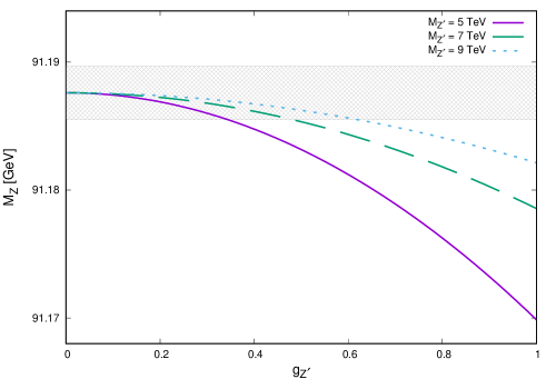
where $g^{2}=g_{2}^{2}+g_{Y}^{2}$. From Eq. 10 we see that the presence of the $Z^{\prime}$ induces corrections on the mass of the SM $Z$ boson. In Fig. 1 we show the impact of these corrections on the SM $Z$ boson mass within the current uncertainties reported in the PDG [60] as a function of $g_{Z^{\prime}}$ for different values of $M_{Z^{\prime}}$. We note that for $g_{Z^{\prime}}\lesssim 0.4$ deviations are well within the current uncertainties.

In the limit where $v_{s}$ is very large, the $Z^{\prime}$ mass decouples and one obtains simplified expressions for the gauge boson masses,

$$M_{Z}^{2}=\frac{1}{4}g^{2}v^{2}\left[1+\mathcal{O}(1/v_{s}^{2})\right]\,,~{}~{}~{}M_{Z^{\prime}}^{2}=\frac{1}{4}N_{z}\left[1+\mathcal{O}(1/v_{s}^{2})\right]$$ (11)

Figure 1: $Z^{\prime}$-induced corrections on the SM $Z$ boson mass as a function of $g_{Z^{\prime}}$ for fixed values of $M_{Z^{\prime}}$. The hatched band represents the current measured $M_{Z}$ uncertainty as reported in the PDG [60].

From the mass matrix diagonalization we obtain the normalized orthogonal eigenvector matrix which is used to rotate the gauge field basis to the physical field basis. The exact form of the elements of this matrix is given in Appendix A. When $v_{s}$ is large, the rotation matrix can be simplified as

$$\begin{pmatrix}W^{3}_{\mu}\\ A^{Y}_{\mu}\\ B_{\mu}\end{pmatrix}=\begin{pmatrix}\sin\theta_{W}&&\cos\theta_{W}\cos\delta&&\cos\theta_{W}\sin\delta\\ \cos\theta_{W}&&-\sin\theta_{W}\cos\delta&&-\sin\theta_{W}\sin\delta\\ 0&&-\sin\delta&&\cos\delta\end{pmatrix}\begin{pmatrix}A^{\gamma}_{\mu}\\ Z_{\mu}\\ Z^{\prime}_{\mu}\end{pmatrix}$$ (12)

where $\theta_{W}$ is the Weinberg angle, $\sin\theta_{W}=g_{2}/g$ and $\cos\theta_{W}=g_{Y}/g$ as in the Standard Model, and the small mixing between the $Z$ and $Z^{\prime}$ is parametrized by the angle $\delta$, defined by

$$\sin\delta=\frac{gx_{z}}{N_{z}-g^{2}v^{2}}+\mathcal{O}\left(\frac{1}{v_{s}^{2}}\right)$$ (13)

To simplify the notation, we define a perturbative parameter $\varepsilon=\sin\delta$. The rotation matrix in Eq. 12 to first order in $\varepsilon$ can now be written as

$$O_{gauge}=\begin{pmatrix}\sin\theta_{W}&\cos\theta_{W}&\varepsilon\cos\theta_{W}\\ \cos\theta_{W}&-\sin\theta_{W}&-\varepsilon\sin\theta_{W}\\ 0&-\varepsilon&1\end{pmatrix}$$ (14)

According to the parameter space explored in this work, $\varepsilon$ is typically $10^{-4}\lesssim\varepsilon\lesssim 10^{-3}$. After fields are rotated to the physical basis, the covariant derivative for the neutral current (NC) sector of Eq. 4 in terms of the mass eigenstate fields is given by

$$\begin{split}{\cal D}_{\mu}^{NC}&=\partial_{\mu}+i\left(g_{2}\sin\theta_{W}\tau^{3}+g_{Y}\cos\theta_{W}\frac{Y}{2}\right)A^{\gamma}_{\mu}\\ &\quad+i\left(g_{2}\cos\theta_{W}\tau^{3}-g_{Y}\sin\theta_{W}\frac{Y}{2}-\varepsilon g_{Z^{\prime}}\frac{z}{2}\right)Z_{\mu}\\ &\quad+i\left(\varepsilon g_{2}\cos\theta_{W}\tau^{3}-\varepsilon g_{Y}\sin\theta_{W}\frac{Y}{2}+g_{Z^{\prime}}\frac{z}{2}\right)Z^{\prime}_{\mu}\end{split}$$ (15)

The neutral current contributions in the Lagrangian, that are of the form $\bar{\psi}\gamma^{\mu}c^{Z}\psi Z_{\mu}$ and $\bar{\psi}\gamma^{\mu}c^{Z^{\prime}}\psi Z^{\prime}_{\mu}$, can be rewritten using the relations $g_{Y}\cos\theta_{W}=g_{2}\sin\theta_{W}$, $Q=\tau^{3}+\frac{Y}{2}$, $e=g_{2}\sin\theta_{W}$

$$c^{Z}=g(\tau^{3}-\sin^{2}\theta_{W}Q)-\varepsilon g_{Z^{\prime}}\frac{z}{2}$$ (16)

$$c^{Z^{\prime}}=\varepsilon g(\tau^{3}-\sin^{2}\theta_{W}Q)+g_{Z^{\prime}}\frac{z}{2}$$

where the charges $\tau^{3},Q,z$ correspond to the fermion and $\varepsilon$ is the (small) mixing parameter. Using this notation, the interactions between fermions and electroweak neutral gauge bosons are expressed in terms of the vector and axial vector couplings, i.e., $\bar{\psi}\gamma^{\mu}\frac{g}{4}\left(g_{V}^{Z}-g_{A}^{Z}\gamma^{5}\right)\psi Z_{\mu}$ and $\bar{\psi}\gamma^{\mu}\frac{g}{4}\left(g_{V}^{Z^{\prime}}-g_{A}^{Z^{\prime}}\gamma^{5}\right)\psi Z^{\prime}_{\mu}$. These couplings are explicitly given as

$$\begin{split}\frac{g}{4}g_{V}^{Z}&=\frac{1}{2}\left[g\left(\tau^{3}_{L}-2\sin^{2}\theta_{W}Q\right)-\varepsilon g_{Z^{\prime}}\left(\frac{z_{L}}{2}+\frac{z_{R}}{2}\right)\right]\\ \frac{g}{4}g_{A}^{Z}&=\frac{1}{2}\left[g\tau^{3}_{L}-\varepsilon g_{Z^{\prime}}\left(\frac{z_{L}}{2}-\frac{z_{R}}{2}\right)\right]\\ \frac{g}{4}g_{V}^{Z^{\prime}}&=\frac{1}{2}\left[\varepsilon g\left(\tau^{3}_{L}-2\sin^{2}\theta_{W}Q\right)+g_{Z^{\prime}}\left(\frac{z_{L}}{2}+\frac{z_{R}}{2}\right)\right]\\ \frac{g}{4}g_{A}^{Z^{\prime}}&=\frac{1}{2}\left[\varepsilon g\tau^{3}_{L}+g_{Z^{\prime}}\left(\frac{z_{L}}{2}-\frac{z_{R}}{2}\right)\right]\\ \end{split}$$ (17)

where $\tau^{3}_{L},z_{L/R}$ refer to left/right-handed fermions.

3.2 Kinetic mixing

In this section we generalize the results obtained in the previous section to the case of kinetic-mixing interactions. The impact of kinetic mixing is assessed in Sec. 4, where applications to hadron collider phenomenology are discussed.

Since the low-energy gauge group includes two abelian groups, the Lagrangian for the kinetic terms can include a contribution which directly couples the $A^{Y}$ and $B$ fields and does not break either $U(1)_{Y}$ or $U(1)_{Z^{\prime}}$ gauge invariance. This term corresponds to gauge kinetic mixing and is of the form

$$\Delta\mathcal{L}_{kin}=-\chi A^{Y}_{\mu\nu}B^{\mu\nu}$$ (18)

where $A^{Y}_{\mu\nu}$ and $B_{\mu\nu}$ are the field-strength tensors for the $U(1)_{Y}$ and $U(1)_{Z^{\prime}}$ symmetry groups respectively, and $\chi$ is a parameter such that $|\chi|<1$. This renormalizable operator plays an interesting role in the context of our model because it can be produced at scales much higher than the $Z^{\prime}$ breaking scale and can affect the couplings of $Z^{\prime}$s at the TeV scale. It is therefore interesting to study the interplay between the gauge kinetic-mixing parameter and coupling of the $Z^{\prime}$. The expression for the electroweak NC covariant derivative is generalized as

$${\cal D}_{\mu}^{NC}=\partial_{\mu}+ig_{2}W^{3}_{\mu}\tau^{3}+iQ^{T}GA$$ (19)

where $Q^{T}=(Y/2,z/2)$ is a vector containing the charges for the two $U(1)$ groups, $G$ is the mixing matrix which is defined as

$$G=\begin{pmatrix}g_{AA}&&g_{AB}\\ g_{BA}&&g_{BB}\end{pmatrix}$$ (20)

and contains the gauge couplings, and $A=(A^{Y}_{\mu},B_{\mu})^{T}$ contains the $U(1)$ gauge fields. The off-diagonal elements $g_{AB}$ and $g_{BA}$ contain the kinetic mixing between the $U(1)$ fields.

It is convenient to perform the rotation $A\rightarrow A^{\prime}=RA$, $G\rightarrow G^{\prime}=GR^{-1}$ where $R$ is an orthogonal $2\times 2$ matrix, and choose $g_{BA}^{\prime}=0$ in order to eliminate the $z_{s}g_{BA}A^{Y}_{\mu}$ term in ${\cal D}_{\mu}^{NC}$. This way, the Higgs singlet does not affect the $SU(2)\times U(1)_{Y}$ sector in the mass matrix. In the new basis, the mixing matrix reads

$$G^{\prime}=\begin{pmatrix}g_{Y}&&g_{KM}\\ 0&&g_{Z^{\prime}}\end{pmatrix}$$ (21)

where

$$g_{Y}=(g_{AA}g_{BB}-g_{AB}g_{BA})/\sqrt{g_{BB}^{2}+g_{AB}^{2}}$$ (22)

$$g_{Z^{\prime}}=\sqrt{g_{BB}^{2}+g_{BA}^{2}}$$

$$g_{KM}=(g_{AA}g_{BA}+g_{AB}g_{BB})/\sqrt{g_{BB}^{2}+g_{BA}^{2}}$$

The electroweak NC covariant derivative becomes

$${\cal D}^{NC}_{\mu}=\partial_{\mu}+ig_{2}W^{3}_{\mu}\tau^{3}+ig_{Y}\frac{Y}{2}A^{Y\prime}_{\mu}+i\left(g_{Z^{\prime}}\frac{z}{2}+g_{KM}\frac{Y}{2}\right)B_{\mu}^{\prime}$$ (23)

where $A^{Y\prime}_{\mu}$ and $B_{\mu}^{\prime}$ are the rotated $U(1)$ gauge fields. Therefore, the inclusion of gauge kinetic mixing can be studied by using a single parameter $g_{KM}$. The mass matrix in the $(W^{3}_{\mu},A^{Y\prime}_{\mu},B_{\mu}^{\prime})$ basis is now

$$\frac{1}{4}\begin{pmatrix}g_{2}^{2}v^{2}&&-g_{2}g_{Y}v^{2}&&g_{2}x_{z}^{\prime}\\ -g_{2}g_{Y}v^{2}&&g_{Y}^{2}v^{2}&&-g_{Y}x_{z}^{\prime}\\ g_{2}x_{z}^{\prime}&&-g_{Y}x_{z}^{\prime}&&N_{z}^{\prime}\end{pmatrix}$$ (24)

where $x_{z}$ and $N_{z}$ have been replaced by their primed expressions given by

$$x_{z}^{\prime}=g_{Z^{\prime}}(z_{H1}v_{1}^{2}-z_{H2}v_{2}^{2})-g_{KM}v^{2}$$ (25)

$$N_{z}^{\prime}=(g_{Z^{\prime}}z_{H1}-g_{KM})^{2}v_{1}^{2}+(g_{Z^{\prime}}z_{H2}+g_{KM})^{2}v_{2}^{2}+g_{Z^{\prime}}^{2}z_{s}^{2}v_{s}^{2}$$

The calculation for the gauge boson masses and the rotation matrix to the physical gauge boson basis proceeds identically to the previous section, with the replacements $x_{z}\rightarrow x_{z}^{\prime}$ and $N_{z}\rightarrow N_{z}^{\prime}$. With these modifications, the general form of the fermionic couplings to the $Z$ and $Z^{\prime}$ in presence of kinetic mixing is

$$c^{Z}=g(\tau^{3}-\sin^{2}\theta_{W}Q)-\varepsilon^{\prime}\left(g_{Z^{\prime}}\frac{z}{2}+g_{KM}\frac{Y}{2}\right)$$ (26)

$$c^{Z^{\prime}}=\varepsilon^{\prime}g(\tau^{3}-\sin^{2}\theta_{W}Q)+g_{Z^{\prime}}\frac{z}{2}+g_{KM}\frac{Y}{2}\,,$$

where the perturbative parameter from the previous section is modified as

$$\varepsilon^{\prime}=\frac{gx_{z}^{\prime}}{N_{z}^{\prime}-g^{2}v^{2}}+\mathcal{O}\left(\frac{1}{v_{s}^{2}}\right)$$ (27)

The vector and axial vector couplings of the gauge bosons to the fermions are now

$$\begin{split}\frac{g}{4}g_{V}^{Z}&=\frac{1}{2}\left[g\left(\tau^{3}_{L}-2\sin^{2}\theta_{W}Q\right)-\varepsilon^{\prime}g_{Z^{\prime}}\left(\frac{z_{L}}{2}+\frac{z_{R}}{2}\right)-\varepsilon^{\prime}g_{KM}\left(\frac{Y_{L}}{2}+\frac{Y_{R}}{2}\right)\right]\\ \frac{g}{4}g_{A}^{Z}&=\frac{1}{2}\left[g\tau^{3}_{L}-\varepsilon^{\prime}g_{Z^{\prime}}\left(\frac{z_{L}}{2}-\frac{z_{R}}{2}\right)-\varepsilon^{\prime}g_{KM}\left(\frac{Y_{L}}{2}-\frac{Y_{R}}{2}\right)\right]\\ \frac{g}{4}g_{V}^{Z^{\prime}}&=\frac{1}{2}\left[\varepsilon^{\prime}g\left(\tau^{3}_{L}-2\sin^{2}\theta_{W}Q\right)+g_{Z^{\prime}}\left(\frac{z_{L}}{2}+\frac{z_{R}}{2}\right)+g_{KM}\left(\frac{Y_{L}}{2}+\frac{Y_{R}}{2}\right)\right]\\ \frac{g}{4}g_{A}^{Z^{\prime}}&=\frac{1}{2}\left[\varepsilon^{\prime}g\tau^{3}_{L}+g_{Z^{\prime}}\left(\frac{z_{L}}{2}-\frac{z_{R}}{2}\right)+g_{KM}\left(\frac{Y_{L}}{2}-\frac{Y_{R}}{2}\right)\right]\\ \end{split}$$ (28)

4 Hadron Collider Phenomenology Applications

In this section we explore the parameter space of the model and perform a detailed analysis for proton-proton collisions at the LHC using Drell-Yan (DY) kinematic distributions calculated at the next-to-next-to-leading order (NNLO) in the strong coupling constant $\alpha_{s}$ of Quantum Chromodynamics (QCD). The contribution of electroweak corrections is not considered here and their impact will be analyzed in a forthcoming work. We explore the sensitivity of the forward-backward asymmetry $(A_{FB})$ distribution to the $Z^{\prime}$ and its parameters. In particular, we use $A_{FB}$ distributions to study the interplay between the gauge kinetic-mixing parameter and coupling of the $Z^{\prime}$. It has been pointed out in several works (e.g., see [17, 18, 19, 20, 21, 22, 23, 24, 25, 26, 27] and references therein) that $A_{FB}$ distributions are very sensitive to SM deviations in the electroweak sector, and in particular to the presence of extra gauge vector bosons. Moreover, the ATLAS, LHCb, and CMS collaborations at the LHC have performed high-precision measurements of $A_{FB}$ distributions at 7, 8, and 13 TeV collision energy respectively [61, 62, 63]. The CMS collaboration [63] has recently set lower limits on the mass of additional gauge bosons from sequential SM extensions at around 4.4 TeV.

Our theory predictions for the DY cross section are complemented by the calculation of uncertainties induced by parton distribution functions (PDFs) in the proton, as well as scale uncertainties for some of the distributions. PDFs represent one of the major sources of uncertainty in cross section calculations and complicate model validation and discrimination. The expression for the DY cross section in QCD factorization can be written as

$$d\sigma=\sum_{ij}\int_{0}^{1}dx_{1}dx_{2}f_{i}^{H_{1}}(x_{1},\mu_{F}^{2})f_{j}^{H_{2}}(x_{2},\mu_{F}^{2})d\hat{\sigma}_{ij\rightarrow l\bar{l}}(x_{1},x_{2};\alpha_{s}(\mu_{R}^{2}),\mu_{R}^{2},\mu_{F}^{2})+{\cal O}\left(\frac{\Lambda_{\textrm{QCD}}^{2}}{Q^{2}}\right)$$ (29)

where $f_{i}^{H_{1}}$ and $f_{j}^{H_{2}}$ are the proton PDFs, which depend on the longitudinal momentum fraction $x_{1}$ and $x_{2}$ of parton $i$ and $j$ respectively, and on the factorization scale $\mu_{F}$. $d\hat{\sigma}$ is the hard scattering cross section, which is perturbatively calculable in QCD, $\mu_{R}$ is the renormalization scale, and $\left(\Lambda_{\textrm{QCD}}^{2}/Q^{2}\right)$ represents power-suppressed contributions where $\Lambda_{\textrm{QCD}}$ is the QCD scale.

The calculation of the differential distributions at NNLO in QCD which we present in this work has been performed by using an amended version of the MCFM-v9.0 computer program [64, 65, 66, 67, 68], which has been modified to incorporate the string-derived model with charge assignments in Table 1, the $Z^{\prime}$ contribution, as well as the interference terms. We validated this implementation against other computer programs such as DY-Turbo [69] and FEWZ [70, 71] and found agreement within 1%. Our results are presented at $\sqrt{S}=$ 13 TeV of center-of-mass energy and we used the CT18NNLO [72] PDFs with conservative uncertainties evaluated at the 90% confidence level (CL). As a case study, we have chosen a string-derived $Z^{\prime}$ with $M_{Z^{\prime}}=$ 5 TeV. The impact of other recent PDF determinations [73, 74, 75] on $A_{FB}$ distributions in the context of extra resonance searches is studied in refs. [26, 27]. Scale uncertainties are obtained by using the 7-point variation, that is, varying $\mu_{R}$ and $\mu_{F}$ up and down independently by a factor of 2, and then taking the envelope.

For the scope of this analysis, it is sufficient to include in the total decay rate of the $Z^{\prime}$ entering the cross section calculation, only the major decay channels which we report in the expression below

$$\Gamma_{Z^{\prime}}=\sum_{f}\Gamma_{Z^{\prime}\rightarrow f\bar{f}}+\Gamma_{Z^{\prime}\rightarrow W^{+}W^{-}}+\Gamma_{Z^{\prime}\rightarrow H^{+}H^{-}}\,,$$ (30)

where $f$ runs over the quarks and leptons, $W^{\pm}$ are the charged gauge vector bosons, and $H^{\pm}$ are the Higgs bosons of the charged sector. The expression for the $\Gamma_{Z^{\prime}\rightarrow H^{+}H^{-}}$ channel in presence of gauge kinetic mixing is given in Appendix B. The calculation of the partial rates relative to the other channels proceeds similarly to that in refs. [57, 59]: in the expression for the $Z^{\prime}$ decay rate in the fermion channel, the vector and axial vector couplings are replaced by those in Eq. 28, while in the expression for the rate in the $W^{+}$ $W^{-}$ channel $\varepsilon$ is replaced by $\varepsilon^{\prime}$ from Eq. 27.

4.1 Kinematic distribution results

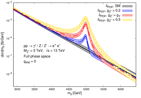
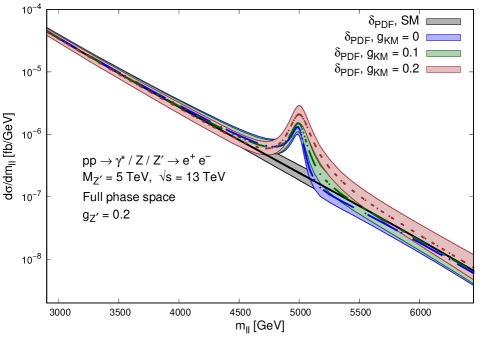
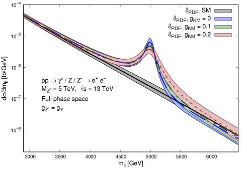
In Fig. 2 we show the string-derived $Z^{\prime}$ results for the dilepton invariant mass ($m_{ll}$) DY spectrum at the LHC 13 TeV in the electron channel, for a $Z^{\prime}$ of mass $M_{Z^{\prime}}$ = 5 TeV and different values of the coupling $g_{Z^{\prime}}$ and kinetic-mixing parameter $g_{KM}$. These theory predictions are compared to the SM and the cross sections are calculated in the full phase space. The error bands represent the CT18NNLO induced PDF uncertainty evaluated at the 90% CL. Central predictions are represented by lines with different dashing. We observe how the interplay between $g_{KM}$ and $g_{Z^{\prime}}$ modifies the shape of the resonance and in particular the width for $g_{Z^{\prime}}=0.2$ and $g_{Z^{\prime}}=g_{Y}$, when the strength of $g_{KM}$ is varied. The inclusion of kinetic mixing has a significant effect on the width of the resonance in the invariant mass distribution.

Figure 2: $Z^{\prime}$ invariant mass distributions for varying $g_{Z^{\prime}}$ and $g_{KM}$. The error bands represent the CT18NNLO induced PDF uncertainty on the cross section at 90% CL. Central predictions are represented by lines with different dashing.

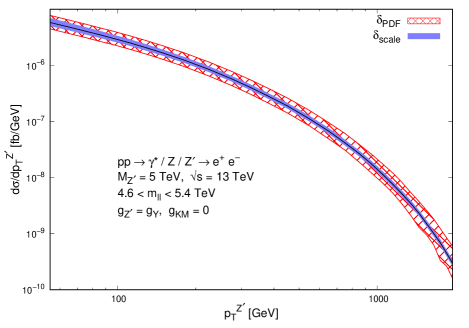
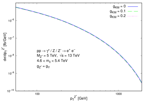
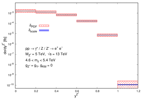
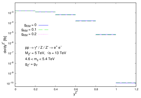
It is interesting to explore the impact of varying these parameters on more differential observables such as the $Z^{\prime}$ transverse momentum $p_{T}$ spectrum and the $Z^{\prime}$ rapidity distribution $y_{Z^{\prime}}$, which we illustrate in Fig. 3. Here, the invariant mass of the final-state dilepton pair is chosen to be $4.6<m_{l\bar{l}}<5.4$ TeV. In the left-column insets, where $g_{KM}=0$, PDF uncertainties are represented by red-hatched bands while scale uncertainties are represented by blue bands. In the right-column insets we illustrate for clarity the same distributions with no uncertainties but with $g_{KM}>0$. We observe that kinetic mixing has negligible impact on these two distributions for this choice of the parameters in the kinematic region $4.6<m_{l\bar{l}}<5.4$ TeV. Again, we observe that PDF uncertainty dominates.

Figure 3: Transverse momentum $p_{T}$ (upper) and rapidity $y_{Z^{\prime}}$ of the $Z^{\prime}$ (lower). The CT18NNLO PDF uncertainty is shown as a hatched red band and scale uncertainty is shown as a solid blue band. Central predictions are represented by a solid black line.

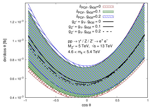
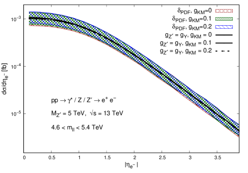
Finally, in Fig. 4 we show the impact of varying the $g_{Z^{\prime}}$ and $g_{KM}$ parameters on the $\cos{\theta}$ distribution, and on the pseudorapidity $\eta_{e}$ spectrum of the final-state electron. The angle $\theta$ is defined in the Collins-Soper frame [76]. While there is almost no impact on the $\eta_{e}$ spectrum, a distortion of the central value of the $\cos\theta$ angular distribution is observed when $g_{KM}$ is progressively increased from 0 to 0.2. As we shall see in the next section, this is reflected by the $A_{FB}$ distribution. However, all these effects in the $\cos{\theta}$ distribution are buried by the almost complete overlap of the PDF uncertainty bands for $g_{KM}=0,0.1,0.2$.

Figure 4: Left: Differential cross-section as a function of $\cos\theta$, where the $\theta$ angle is defined in the Collins-Soper frame. Right: Pseudorapidity distribution $\eta_{e}$ of the outgoing electron. Error bands with different hatching represent the CT18NNLO PDF uncertainties induced on the cross section, evaluated at the 90% CL. Central predictions are represented by lines with different dashing.

4.2 Forward-Backward Asymmetry $A_{FB}$ distribution results

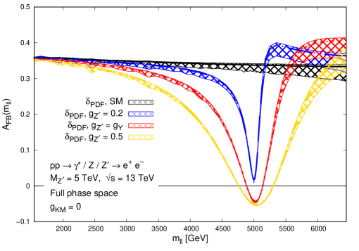
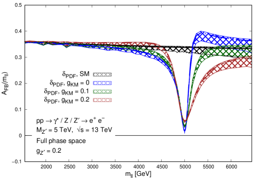
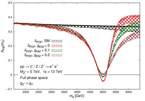
As anticipated in the previous sections, a more suitable variable to explore the $Z^{\prime}$ parameters in DY is the forward-backward asymmetry $A_{FB}$ distribution. This observable is a function of the chiral quark and lepton couplings to the mediating gauge bosons and is very sensitive to $Z^{\prime}$ properties. $A_{FB}$ is expressed in terms of the difference between the forward and backward angular contributions to the cross section, normalized to the total cross section. The forward and backward directions are represented by the angle $\theta$ between the negatively charged final-state lepton and the initial-state quark in the dilepton center-of-mass frame. $A_{FB}$ is defined as

$$A_{FB}=\frac{d\sigma_{F}-d\sigma_{B}}{d\sigma_{F}+d\sigma_{B}}$$ (31)

where the forward ($d\sigma_{F}$) and backward ($d\sigma_{B}$) contributions are constructed by integrating the differential cross section over the forward and backward halves of the angular phase space

$$d\sigma_{F}=\int_{0}^{1}\frac{d\sigma}{d\cos{\theta_{l}}}\,d\cos{\theta_{l}},\;\;\;d\sigma_{B}=\int_{-1}^{0}\frac{d\sigma}{d\cos{\theta_{l}}}\,d\cos{\theta_{l}}\,.$$ (32)

$\theta_{l}$ is the angle between the final-state lepton and initial-state quark in the Collins-Soper frame. In our analysis, we study the $A_{FB}$ distribution as a function of $m_{ll}$. In Fig. 5 we show the $A_{FB}$ over the same invariant mass range adopted before. The presence of a $Z^{\prime}$ would lead to a distortion in the $A_{FB}$ which becomes wider as $g_{Z^{\prime}}$ increases. We calculated both PDF and scale uncertainties for the $A_{FB}$ distribution. Scale uncertainties are essentially invisible in Fig. 5, while PDF uncertainties are attenuated around the peak as compared to the distributions studied in the previous section, but are still large at high $m_{ll}$. Fig. 5 shows the sensitivity of $A_{FB}$ to simultaneous variations of the $g_{Z^{\prime}}$ and $g_{KM}$ parameters. The distortions induced on the asymmetry tend to become shallower and wider as the kinetic mixing increases. Moving away from the resonance, when $g_{KM}\neq 0$, the discriminatory power of $A_{FB}$ appears to be attenuated by PDF uncertainties.

Figure 5: Forward-backward asymmetry ($A_{FB}$) shown as a function of the dilepton invariant mass ($m_{ll}$) for different values of $g_{Z^{\prime}}$ and $g_{KM}$. The black hatched band represents the Standard Model prediction. The solid black line at $A_{FB}=0$ is introduced for reference. The CT18NNLO PDF uncertainties at the 90% CL are represented by hatched bands. Central predictions are shown as lines with different dashing.

5 Conclusions

In this work, we studied properties of heterotic string derived $Z^{\prime}$s in the TeV scale and explored their dynamics at the LHC. As a case study, we selected a $Z^{\prime}$ of mass $M_{Z^{\prime}}=5$ TeV. We analyzed the impact of a gauge kinetic-mixing term in the Lagrangian and its interplay with the $Z^{\prime}$ coupling. We explored the $Z^{\prime}$ parameter space the model in presence of kinetic mixing and performed a thorough phenomenological analysis in which we used precision calculations at NNLO in QCD to predict kinematic distributions for the $Z^{\prime}$ in the Drell-Yan process at the LHC. In particular, we exploited the sensitivity of forward-backward asymmetry $A_{FB}$ distributions in Drell-Yan to further explore the parameter space and the interplay between the $Z^{\prime}$ coupling and the kinetic-mixing parameter. Moreover, we estimated theory uncertainties on the distributions from perturbative (scale dependence) and nonperturbative (PDFs in the proton) sources in QCD. Proton PDFs still remain one of the major sources of uncertainty in $Z^{\prime}$ searches. This is ascribed to the fact that the kinematic domain of heavy gauge boson production is sensitive, and is impacted by, PDFs at large $x$ where uncertainties are still large due to lack of robust constraints from experimental data [77, 78]. The motivation to consider the particular $U(1)_{Z^{\prime}}$ combination in Eq. 3 stems from its extraction from a string derived heterotic–string model [9], in which it is the unique combination that may remain unbroken down to low scales. Its preservation as an unbroken gauge symmetry down to the TeV scale emanates from the role that it can play in suppressing some dangerous operators, like proton decay mediating operators, and furthermore by the role it can play in generating the electroweak symmetry breaking itself. Further analysis in that direction mandates the development of the interpolation tools between the string and electroweak scales and the extraction of further data from the string models. We note that while in this paper we treated the kinetic-mixing term as a free parameter, its computation, as that of many of the related parameters, can be obtained directly from the string models [15], hence increasing their predictive power. In this paper, we studied the case of $Z^{\prime}$ vector bosons that have an $E_{6}$ embedding. The advantage of this choice is that it facilitates gauge unification at the unification scale [8]. Such extra string inspired $Z^{\prime}$ models have been discussed extensively in the literature since the mid–eighties [32, 19, 33, 34], but the combination given in Eq. 3 is obtained in the string derived model of ref. [9]. Naturally, the string constructions can give rise to $U(1)$ symmetries with different characteristics and these have been of some interest in the literature [36, 37, 38, 7]. The range of possibilities is more model dependent. The extra $Z^{\prime}$s in these cases can arise from flavour dependent $U(1)$ symmetries, as well as $U(1)$ symmetries that arise from the hidden sector of the heterotic–string. Naturally, the limits that we discussed in this paper will not apply to those cases (see for instance the discussion relative to $Z^{\prime}$ boson searches in the PDG [60] and references therein), as they do not couple universally to all the three families. On the other hand, there may exist other constraints in these cases arising from flavour non–universality and the need to break flavour dependent symmetries to produce viable fermion masses. Nevertheless, these cases do represent interesting alternatives to the family universal $U(1)$ and we will return to them in future work.

Acknowledgments

The work of MG and AM is supported by the National Science foundation under Grant no. 2112025. The work of AF is supported in part by a Weston visiting professorship at the Weizmann Institute of Science. AF would like to thank Doron Gepner for discussions and the Department of Particle Physics and Astrophysics for hospitality.

Appendix A Gauge boson rotation matrix components

In this section we report the exact components of the matrix $\mathcal{O}_{gauge}$ which rotates the neutral gauge field basis to the physical basis as in Eq. 12.

$$\begin{split}&\mathcal{O}_{11}=g_{Y}/g,\quad\mathcal{O}_{21}=g_{2}/g,\quad\mathcal{O}_{31}=0,\\ &\mathcal{O}_{12}=-g_{2}\frac{v^{2}\left(f_{1}+\sqrt{f_{1}^{2}+4g^{2}x_{z}^{2}}\right)-2x_{z}^{2}}{\sqrt{g^{2}\left[v^{2}\left(f_{1}+\sqrt{f_{1}^{2}+4g^{2}x_{z}^{2}}\right)-2x_{z}^{2}\right]^{2}+x_{z}^{2}\left(f_{2}-\sqrt{f_{1}^{2}+4g^{2}x_{z}^{2}}\right)^{2}}},\\ &\mathcal{O}_{22}=g_{Y}\frac{v^{2}\left(f_{1}+\sqrt{f_{1}^{2}+4g^{2}x_{z}^{2}}\right)-2x_{z}^{2}}{\sqrt{g^{2}\left[v^{2}\left(f_{1}+\sqrt{f_{1}^{2}+4g^{2}x_{z}^{2}}\right)-2x_{z}^{2}\right]^{2}+x_{z}^{2}\left(f_{2}-\sqrt{f_{1}^{2}+4g^{2}x_{z}^{2}}\right)^{2}}},\\ &\mathcal{O}_{32}=\frac{x_{z}\left(f_{2}-\sqrt{f_{1}^{2}+4g^{2}x_{z}^{2}}\right)}{\sqrt{g^{2}\left[v^{2}\left(f_{1}+\sqrt{f_{1}^{2}+4g^{2}x_{z}^{2}}\right)-2x_{z}^{2}\right]^{2}+x_{z}^{2}\left(f_{2}-\sqrt{f_{1}^{2}+4g^{2}x_{z}^{2}}\right)^{2}}},\\ &\mathcal{O}_{13}=-g_{2}\frac{v^{2}\left(f_{1}-\sqrt{f_{1}^{2}+4g^{2}x_{z}^{2}}\right)-2x_{z}^{2}}{\sqrt{g^{2}\left[v^{2}\left(f_{1}-\sqrt{f_{1}^{2}+4g^{2}x_{z}^{2}}\right)-2x_{z}^{2}\right]^{2}+x_{z}^{2}\left(f_{2}+\sqrt{f_{1}^{2}+4g^{2}x_{z}^{2}}\right)^{2}}},\\ &\mathcal{O}_{23}=g_{Y}\frac{v^{2}\left(f_{1}-\sqrt{f_{1}^{2}+4g^{2}x_{z}^{2}}\right)-2x_{z}^{2}}{\sqrt{g^{2}\left[v^{2}\left(f_{1}-\sqrt{f_{1}^{2}+4g^{2}x_{z}^{2}}\right)-2x_{z}^{2}\right]^{2}+x_{z}^{2}\left(f_{2}+\sqrt{f_{1}^{2}+4g^{2}x_{z}^{2}}\right)^{2}}},\\ &\mathcal{O}_{33}=\frac{x_{z}\left(f_{2}+\sqrt{f_{1}^{2}+4g^{2}x_{z}^{2}}\right)}{\sqrt{g^{2}\left[v^{2}\left(f_{1}-\sqrt{f_{1}^{2}+4g^{2}x_{z}^{2}}\right)-2x_{z}^{2}\right]^{2}+x_{z}^{2}\left(f_{2}+\sqrt{f_{1}^{2}+4g^{2}x_{z}^{2}}\right)^{2}}}\end{split}$$ (A1)

where $f_{1}=N_{z}-g^{2}v^{2}$ and $f_{2}=N_{z}+g^{2}v^{2}$. To include the effects of kinetic mixing on $\mathcal{O}_{gauge}$, we make the substitutions $x_{z}\rightarrow x_{z}^{\prime}$ and $N_{z}\rightarrow N_{z}^{\prime}$ as defined in Eq. 25.

Appendix B $Z^{\prime}\rightarrow H^{+}H^{-}$ decay rate

The decay rate of the $Z^{\prime}$ into charged Higgs bosons $Z^{\prime}\rightarrow H^{+}H^{-}$ in presence of kinetic mixing is given by

$$\Gamma_{Z^{\prime}\rightarrow H^{+}H^{-}}=\frac{g^{2}_{Z^{\prime}H^{+}H^{-}}}{16\pi^{2}M_{Z^{\prime}}^{5}}\left[M_{Z^{\prime}}^{2}(M_{Z^{\prime}}-2M_{H^{\pm}})(2M_{H^{\pm}}+M_{Z^{\prime}})\right]^{3/2},$$ (33)

where the structure of the coupling is

$$\begin{split}g_{Z^{\prime}H^{+}H^{-}}=&\left(\frac{v_{1}}{v}\right)^{2}(g_{Z^{\prime}}z_{H_{1}}+\varepsilon g_{2}\cos\theta_{W})+\left(\frac{v_{2}}{v}\right)^{2}(-g_{Z^{\prime}}z_{H_{2}}+\varepsilon g_{2}\cos\theta_{W})\\ &+(g_{KM}+\varepsilon g_{Y}\sin\theta_{W})\left(\left(\frac{v_{1}}{v}\right)^{2}Y_{H_{1}}-\left(\frac{v_{2}}{v}\right)^{2}Y_{H_{2}}\right).\end{split}$$ (34)

References

- [1] L. E. Ibanez and A. M. Uranga, String theory and particle physics: An introduction to string phenomenology. Cambridge University Press, 2, 2012.
- [2] A. E. Faraggi, D. V. Nanopoulos and K.-j. Yuan, A Standard Like Model in the 4D Free Fermionic String Formulation, Nucl. Phys. B 335 (1990) 347.
- [3] G. B. Cleaver, A. E. Faraggi and D. V. Nanopoulos, String derived MSSM and M theory unification, Phys. Lett. B 455 (1999) 135 [hep-ph/9811427].
- [4] A. E. Faraggi, Construction of realistic standard - like models in the free fermionic superstring formulation, Nucl. Phys. B 387 (1992) 239 [hep-th/9208024].
- [5] A. E. Faraggi, J. Rizos and H. Sonmez, Classification of standard-like heterotic-string vacua, Nucl. Phys. B 927 (2018) 1 [1709.08229].
- [6] P. Athanasopoulos, A. E. Faraggi, S. Groot Nibbelink and V. M. Mehta, Heterotic free fermionic and symmetric toroidal orbifold models, JHEP 04 (2016) 038 [1602.03082].
- [7] A. E. Faraggi and V. M. Mehta, Proton Stability and Light Inspired by String Derived Models, Phys. Rev. D 84 (2011) 086006 [1106.3082].
- [8] A. E. Faraggi and V. M. Mehta, Proton stability, gauge coupling unification, and a light Z’ in heterotic-string models, Phys. Rev. D 88 (2013) 025006 [1304.4230].
- [9] A. E. Faraggi and J. Rizos, A light Z’ heterotic-string derived model, Nucl. Phys. B 895 (2015) 233 [1412.6432].
- [10] Y. Y. Komachenko and M. Y. Khlopov, On Manifestation of Boson of Heterotic String in Exclusive Neutrino Neutrino P0 Processes, Sov. J. Nucl. Phys. 51 (1990) 692. Yad.Fiz. 51 (1990) 1081.
- [11] A. Das, P. S. B. Dev, Y. Hosotani, S. Mandal, Probing the minimal model at future electron-positron colliders via fermion pair-production channels, Phys. Rev. D 105 (2022) 115030 [2104.10902].
- [12] P. Anastasopoulos, F. Fucito, A. Lionetto, G. Pradisi, A. Racioppi, Y. Stanev. Minimal Anomalous Extension of the MSSM Phys. Rev. D 78 (2008) 085014 [0804.1156].
- [13] B. Holdom, Two U(1)’s and Epsilon Charge Shifts, Phys. Lett. B 166 (1986) 196.
- [14] J. Polchinski and L. Susskind, Breaking of Supersymmetry at Intermediate-Energy, Phys. Rev. D 26 (1982) 3661.
- [15] K. R. Dienes, C. F. Kolda and J. March-Russell, Kinetic mixing and the supersymmetric gauge hierarchy, Nucl. Phys. B 492 (1997) 104 [hep-ph/9610479].
- [16] T. G. Rizzo, Gauge kinetic mixing and leptophobic in E(6) and SO(10), Phys. Rev. D 59 (1998) 015020 [hep-ph/9806397].
- [17] D. London and J. L. Rosner, Extra Gauge Bosons in E(6), Phys. Rev. D 34 (1986) 1530.
- [18] J. L. Rosner, Off Peak Lepton Asymmetries From New s, Phys. Rev. D 35 (1987) 2244.
- [19] J. L. Hewett and T. G. Rizzo, Low-Energy Phenomenology of Superstring Inspired E(6) Models, Phys. Rept. 183 (1989) 193.
- [20] M. Cvetic and S. Godfrey, Discovery and identification of extra gauge bosons, Advanced Series on Directions in High Energy Physics 16 (1997) 383 [hep-ph/9504216].
- [21] J. L. Rosner, Forward - backward asymmetries in hadronically produced lepton pairs, Phys. Rev. D 54 (1996) 1078 [hep-ph/9512299].
- [22] M. Dittmar, Neutral current interference in the TeV region: The Experimental sensitivity at the LHC, Phys. Rev. D 55 (1997) 161 [hep-ex/9606002].
- [23] A. Bodek and U. Baur, Implications of a 300-GeV/c to 500-Gev/c boson on antip collider data at = 1.8 TeV, Eur. Phys. J. C 21 (2001) 607 [hep-ph/0102160].
- [24] CDF collaboration, F. Abe et al., Search for new gauge bosons decaying into dileptons in collisions at TeV, Phys. Rev. Lett. 79 (1997) 2192.
- [25] E. Accomando, A. Belyaev, J. Fiaschi, K. Mimasu, S. Moretti and C. Shepherd-Themistocleous, Forward-backward asymmetry as a discovery tool for Z’ bosons at the LHC, JHEP 01 (2016) 127 [1503.02672].
- [26] J. Fiaschi, F. Giuli, F. Hautmann, S. Moch and S. Moretti, -boson dilepton searches and the high- quark density, 2211.06188.
- [27] R. D. Ball, A. Candido, S. Forte, F. Hekhorn, E. R. Nocera, J. Rojo et al., Parton Distributions and New Physics Searches: the Drell-Yan Forward-Backward Asymmetry as a Case Study, 2209.08115.
- [28] I. Antoniadis, C. P. Bachas and C. Kounnas, Four-Dimensional Superstrings, Nucl. Phys. B 289 (1987) 87.
- [29] H. Kawai, D. C. Lewellen and S. H. H. Tye, Construction of Fermionic String Models in Four-Dimensions, Nucl. Phys. B 288 (1987) 1.
- [30] I. Antoniadis and C. Bachas, 4-D Fermionic Superstrings with Arbitrary Twists, Nucl. Phys. B 298 (1988) 586.
- [31] P. Candelas, G. T. Horowitz, A. Strominger and E. Witten, Vacuum Configurations for Superstrings, Nucl. Phys. B 258 (1985) 46.
- [32] F. Zwirner, Phenomenological aspects of superstring-inspired models, Int. J. Mod. Phys. A 3 (1988) 49.
- [33] A. Leike, The Phenomenology of extra neutral gauge bosons, Phys. Rept. 317 (1999) 143 [hep-ph/9805494].
- [34] S. F. King, S. Moretti and R. Nevzorov, A Review of the Exceptional Supersymmetric Standard Model, Symmetry 12 (2020) 557 [2002.02788].
- [35] G. B. Cleaver and A. E. Faraggi, On the anomalous U(1) in free fermionic superstring models, Int. J. Mod. Phys. A 14 (1999) 2335 [hep-ph/9711339].
- [36] J. C. Pati, The Essential role of string derived symmetries in ensuring proton stability and light neutrino masses, Phys. Lett. B 388 (1996) 532 [hep-ph/9607446].
- [37] A. E. Faraggi, Proton stability and superstring Z-prime, Phys. Lett. B 499 (2001) 147 [hep-ph/0011006].
- [38] C. Corianò, A. E. Faraggi and M. Guzzi, A Novel string derived Z-prime with stable proton, light-neutrinos and R-parity violation, Eur. Phys. J. C 53 (2008) 421 [0704.1256].
- [39] A. E. Faraggi and D. V. Nanopoulos, A SUPERSTRING AT O (1-TeV) ?, Mod. Phys. Lett. A 6 (1991) 61.
- [40] A. E. Faraggi, Mass as Possible Evidence for a Superstring Inspired Standard Like Model, Phys. Lett. B 245 (1990) 435.
- [41] L. Bernard, A. E. Faraggi, I. Glasser, J. Rizos and H. Sonmez, String Derived Exophobic GUTs, Nucl. Phys. B 868 (2013) 1 [1208.2145].
- [42] A. E. Faraggi, C. Kounnas and J. Rizos, Spinor-Vector Duality in fermionic heterotic orbifold models, Nucl. Phys. B 774 (2007) 208 [hep-th/0611251].
- [43] C. Angelantonj, A. E. Faraggi and M. Tsulaia, Spinor-Vector Duality in Heterotic String Orbifolds, JHEP 07 (2010) 004 [1003.5801].
- [44] A. E. Faraggi, I. Florakis, T. Mohaupt and M. Tsulaia, Conformal Aspects of Spinor-Vector Duality, Nucl. Phys. B 848 (2011) 332 [1101.4194].
- [45] A. E. Faraggi, C. Kounnas, S. E. M. Nooij and J. Rizos, Classification of the chiral Z(2) x Z(2) fermionic models in the heterotic superstring, Nucl. Phys. B 695 (2004) 41 [hep-th/0403058].
- [46] B. Assel, K. Christodoulides, A. E. Faraggi, C. Kounnas and J. Rizos, Classification of Heterotic Pati-Salam Models, Nucl. Phys. B 844 (2011) 365 [1007.2268].
- [47] A. Faraggi, J. Rizos and H. Sonmez, Classification of Flipped SU(5) Heterotic-String Vacua, Nucl. Phys. B 886 (2014) 202 [1403.4107].
- [48] A. E. Faraggi, G. Harries and J. Rizos, Classification of left–right symmetric heterotic string vacua, Nucl. Phys. B 936 (2018) 472 [1806.04434].
- [49] A. E. Faraggi, G. Harries, B. Percival and J. Rizos, Doublet-Triplet Splitting in Fertile Left-Right Symmetric Heterotic String Vacua, Nucl. Phys. B 953 (2020) 114969 [1912.04768].
- [50] A. E. Faraggi, V. G. Matyas and B. Percival, Towards the Classification of Tachyon-Free Models From Tachyonic Ten-Dimensional Heterotic String Vacua, Nucl. Phys. B 961 (2020) 115231 [2006.11340].
- [51] A. E. Faraggi, V. G. Matyas and B. Percival, Classification of nonsupersymmetric Pati-Salam heterotic string models, Phys. Rev. D 104 (2021) 046002 [2011.04113].
- [52] I. Antoniadis and G. K. Leontaris, A supersymmetric model, Phys. Lett. B 216 (1989) 333.
- [53] A. E. Faraggi, Sterile Neutrinos in String Derived Models, Eur. Phys. J. C 78 (2018) 867 [1807.08031].
- [54] A. E. Faraggi, Proton stability in superstring derived models, Nucl. Phys. B 428 (1994) 111 [hep-ph/9403312].
- [55] A. E. Faraggi, Doublet triplet splitting in realistic heterotic string derived models, Phys. Lett. B 520 (2001) 337 [hep-ph/0107094].
- [56] L. Delle Rose, A. E. Faraggi, C. Marzo and J. Rizos, Wilsonian dark matter in string derived model, Phys. Rev. D 96 (2017) 055025 [1704.02579].
- [57] A. E. Faraggi and M. Guzzi, s and sterile neutrinos from heterotic string models: exploring mass exclusion limits, Eur. Phys. J. C 82 (2022) 590 [2204.11974].
- [58] A. E. Faraggi and M. Guzzi, Extra s and s in heterotic-string derived models, Eur. Phys. J. C75 (2015) 537 [1507.07406].
- [59] C. Corianò, A. E. Faraggi and M. Guzzi, Searching for Extra Z-prime from Strings and Other Models at the LHC with Leptoproduction, Phys. Rev. D 78 (2008) 015012 [0802.1792].
- [60] Particle Data Group collaboration, R. L. Workman et al., Review of Particle Physics, PTEP 2022 (2022) 083C01.
- [61] ATLAS collaboration, G. Aad et al., Measurement of the forward-backward asymmetry of electron and muon pair-production in collisions at = 7 TeV with the ATLAS detector, JHEP 09 (2015) 049 [1503.03709].
- [62] LHCb collaboration, R. Aaij et al., Measurement of the forward-backward asymmetry in decays and determination of the effective weak mixing angle, JHEP 11 (2015) 190 [1509.07645].
- [63] CMS collaboration, A. Tumasyan et al., Measurement of the Drell-Yan forward-backward asymmetry at high dilepton masses in proton-proton collisions at = 13 TeV, JHEP 2022 (2022) 063 [2202.12327].
- [64] J. M. Campbell and R. K. Ellis, An Update on vector boson pair production at hadron colliders, Phys. Rev. D 60 (1999) 113006 [hep-ph/9905386].
- [65] J. M. Campbell, R. K. Ellis and C. Williams, Vector boson pair production at the LHC, JHEP 07 (2011) 018 [1105.0020].
- [66] J. M. Campbell, R. K. Ellis and W. T. Giele, A Multi-Threaded Version of MCFM, Eur. Phys. J. C 75 (2015) 246 [1503.06182].
- [67] R. Boughezal, J. M. Campbell, R. K. Ellis, C. Focke, W. Giele, X. Liu et al., Color singlet production at NNLO in MCFM, Eur. Phys. J. C 77 (2017) 7 [1605.08011].
- [68] J. Campbell and T. Neumann, Precision Phenomenology with MCFM, JHEP 12 (2019) 034 [1909.09117].
- [69] S. Camarda et al., DYTurbo: Fast predictions for Drell-Yan processes, Eur. Phys. J. C 80 (2020) 251 [1910.07049].
- [70] R. Gavin, Y. Li, F. Petriello and S. Quackenbush, FEWZ 2.0: A code for hadronic Z production at next-to-next-to-leading order, Comput. Phys. Commun. 182 (2011) 2388 [1011.3540].
- [71] Y. Li and F. Petriello, Combining QCD and electroweak corrections to dilepton production in FEWZ, Phys. Rev. D 86 (2012) 094034 [1208.5967].
- [72] T.-J. Hou et al., New CTEQ global analysis of quantum chromodynamics with high-precision data from the LHC, 1912.10053.
- [73] S. Alekhin, J. Blümlein, S. Moch and R. Placakyte, Parton distribution functions, , and heavy-quark masses for LHC Run II, Phys. Rev. D 96 (2017) 014011 [1701.05838].
- [74] S. Bailey, T. Cridge, L. A. Harland-Lang, A. D. Martin and R. S. Thorne, Parton distributions from LHC, HERA, Tevatron and fixed target data: MSHT20 PDFs, Eur. Phys. J. C 81 (2021) 341 [2012.04684].
- [75] NNPDF collaboration, R. D. Ball et al., The path to proton structure at 1% accuracy, Eur. Phys. J. C 82 (2022) 428 [2109.02653].
- [76] J. C. Collins and D. E. Soper, Angular Distribution of Dileptons in High-Energy Hadron Collisions, Phys. Rev. D 16 (1977) 2219.
- [77] L. T. Brady, A. Accardi, W. Melnitchouk and J. F. Owens, Impact of PDF uncertainties at large x on heavy boson production, JHEP 06 (2012) 019 [1110.5398].
- [78] S. Amoroso et al., Snowmass 2021 whitepaper: Proton structure at the precision frontier, 2203.13923.