On Robust Learning from Noisy Labels: A Permutation Layer Approach

Abstract

The existence of label noise imposes significant challenges (e.g., poor generalization) on the training process of deep neural networks (DNN). As a remedy, this paper introduces a permutation layer learning approach termed PermLL to dynamically calibrate the training process of the DNN subject to instance-dependent and instance-independent label noise. The proposed method augments the architecture of a conventional DNN by an instance-dependent permutation layer. This layer is essentially a convex combination of permutation matrices that is dynamically calibrated for each sample. The primary objective of the permutation layer is to correct the loss of noisy samples mitigating the effect of label noise. We provide two variants of PermLL in this paper: one applies the permutation layer to the model’s prediction, while the other applies it directly to the given noisy label. In addition, we provide a theoretical comparison between the two variants and show that previous methods can be seen as one of the variants. Finally, we validate PermLL experimentally and show that it achieves state-of-the-art performance on both real and synthetic datasets.

1 Introduction

Deep Neural Networks (DNNs) have achieved outstanding performance on many vision problems, including image classification (Krizhevsky, Sutskever, and Hinton 2012), object detection (Redmon et al. 2016), semantic segmentation (Long, Shelhamer, and Darrell 2015), and scene labeling (Farabet et al. 2012). The success in these challenges heavily relies on the availability of huge and correctly labeled datasets, which are very expensive and time-demanding to collect. To overcome this challenge, a number of crowdsourcing platforms such as Amazon’s Mechanical Turk and nonexpert sources such as Internet Web Images, where labels are inferred by surrounding text or keywords, have been developed over the past years (Xiao et al. 2015a). Although these methods reduce the labeling cost, the labels derived from these techniques are unreliable due to the high noise rate caused by human annotators or extraction algorithms (Paolacci, Chandler, and Ipeirotis 2010; Scott, Blanchard, and Handy 2013). In addition, more challenging tasks usually require domain expert annotators and thus are highly prone to mislabeling (Frénay and Verleysen 2013; Lloyd et al. 2004), such as breast tumor classification (Lee et al. 2018).

Training on such noisy datasets negatively impacts the performance of DDNs (i.e., poor generalization) due to the memorization effect (Maennel et al. 2020). Interestingly, the authors in (Zhang et al. 2021) illustrated that DNNs can easily fit randomly labeled training data. This property is especially problematic when training in the presence of label noise since typical DNNs tend to memorize the noisy instances leading to a subpar classifier.

To overcome this impediment, we propose a learnable permutation layer that is applied to one of the training loss arguments (i.e., model prediction or label). Each training sample has an independent permutation layer associated with a learnable parameter $\boldsymbol{\alpha}$. The purpose of the permutation layer is to correct the loss of noisy samples through permuting predictions or labels during training, allowing the model to learn safely from them. During inference, the permutation layer is discarded. Our contributions can be summarized as follows:

1. We propose a permutation layer learning framework PermLL that can effectively learn from datasets containing noisy labels.

2. We theoretically analyze two variants of PermLL. The first approach applies the permutation layer to the predictions, while the second applies the permutation to the labels. We show that the approach of learning the labels directly, proposed in Joint Optimization (Tanaka et al. 2018), can be seen as a special case of PermLL.

3. We provide a theoretical analysis of the two proposed methods, showing that applying the permutation layer to the predictions has better theoretical properties.

4. We empirically demonstrate the effectiveness of PermLL on synthetic and real noise, achieving state-of-the-art performance on CIFAR-10, CIFAR-100, and Clothing1M.

2 Related Work

In recent years, a considerable number of methods have been proposed to deal with different types of label noise. Label noise can come from a closed-set or an open-set. In the closed-set case, the true label of a noisy sample is guaranteed to belong to the dataset’s predefined set of labels, while in the open-set noise the true label could fall outside the predefined labels. Under closed-set noise, the label noise can be further categorized into instance-independent label noise and instance-dependent label noise (Natarajan et al. 2013; Xiao et al. 2015a). For instance-independent label noise, the noise is conditionally independent on the sample feature given its clean label. Therefore, the label noise can be characterized as a transition matrix (Frénay and Verleysen 2013). Instance-dependent label noise, on the other hand, depends on both sample features and the true label (Xiao et al. 2015a). In this paper, we only consider a closed-set noise setting, covering both instance-dependent and instance-independent noise.

Many methods have been proposed to learn robustly from noisy labeled datasets. These methods can be categorized based on how they handle corrupted samples into sample selection and loss correction methods. The reader may refer to (Song et al. 2022; Frénay and Verleysen 2013) for a more thorough review.

Sample selection.

Sample selection methods provide a heuristic to isolate clean samples from noisy ones. Then, the noisy samples are either discarded or used as unlabeled samples in a semi-supervised manner (Malach and Shalev-Shwartz 2017; Han et al. 2018; Yu et al. 2019; Li, Socher, and Hoi 2020; Song et al. 2021). To name a few, Decouple (Malach and Shalev-Shwartz 2017) trains two networks on samples where they have disagreements in the prediction. Co-teaching (Han et al. 2018) uses two networks, each selecting small-loss samples in a mini-batch to train the other. Inspired by Decouple, Co-teaching+ (Yu et al. 2019) improves on Co-teaching by training two networks on samples that have small-loss and prediction disagreement. Unlike these methods, our work follows a loss correction approach.

Loss correction

Methods of this type cope with label noise by correcting the loss of noisy samples. Therefore, this line of work is more relevant to our approach. Several methods modify the loss function by augmenting their model with a linear layer during training. Some works utilize an estimated transition matrix to correct the loss (Patrini et al. 2017a; Hendrycks et al. 2018; Xia et al. 2019; Yao et al. 2020). Notably, (Patrini et al. 2017a) first estimates the noise transition matrix using the model’s predictions in an initial training phase. Then, the model is re-trained with either a forward or backward correction. The performance of such methods highly depends on the quality of the estimated transition matrix. Similarly, other methods augment their models with a noise adaptation layer (Chen and Gupta 2015; Sukhbaatar et al. 2014). Unlike transition matrix-based methods, the adaptation layer is learned simultaneously with the model. A major drawback of the previously mentioned methods, using a transition matrix or an adaptation layer, is that they treat all samples equally. PermLL, however, employs an instance-dependent permutation layer that can deal with samples differently.

Another prominent line of work mitigates the effect of label noise by refurbishing the labels. For example, Bootstrapping (Reed et al. 2014) generates training targets that are obtained by a convex combination of the model prediction and the noisy labels using a single parameter $\beta$ for all samples. To remedy this, (Arazo et al. 2019) dynamically adjusts the parameter $\beta$ for every sample using a beta mixture model fitted to the training loss of each sample. Such bootstrapping techniques require careful hyperparameter scheduling, increasing their complexity. Joint Optimization (Tanaka et al. 2018) proposes a more straightforward approach that jointly learns the model’s parameters and the labels. In addition, (Tanaka et al. 2018) uses regularization terms to impose a known prior distribution on the labels and to avoid getting stuck in local optima. Inspired by (Tanaka et al. 2018), PENCIL (Yi and Wu 2019) learns label distributions instead of constant labels.

In contrast to the aforementioned literature, our proposed method employs a learnable instance-dependent permutation layer that is applied to one of the training loss arguments (i.e., model prediction or label). From the previously mentioned methods, Joint Optimization (Tanaka et al. 2018) is the most relevant to our work. However, instead of learning the labels, we learn instance-dependent permutation layers. In addition, we are different in several other aspects: i) our method works well without any regularization terms and thus has fewer hyperparameters. ii) Unlike (Tanaka et al. 2018), we are not limited to datasets with only few classes. iii) (Tanaka et al. 2018) is, in fact, a special case of our formulation.

3 Methodology

We develop a learning scheme that is robust to label noise. In our treatment, we consider c-class classification problems. Given a noisy training data $D:=\big{\{}(\mathbf{x}^{i},\tilde{y}^{i})\big{\}}_{i=1}^{N}$ where $\mathbf{x}^{i}\in\mathbb{R}^{m}$ are the input features, $\tilde{y}^{i}\in\{1,...,c\}$ is the noisy label, and $N$ is the number of training samples, we aim to learn a classifier $f_{\theta}$ on $D$ while mitigating the impact of label noise.

Notation.

Consider a classifier $f_{\theta}:\mathbb{R}^{m}\rightarrow p(c)$, where $p(c)$ is a probability simplex over c classes, i.e., $p(c)=\{\mathbf{z}\in\mathbb{R}^{c}\,|\,\mathbf{z}\geq\mathbf{0},\,\mathbf{1}^{T}\mathbf{z}=1\}$. Let $P(i,j)$ be an elementary permutation matrix that permutes the $i^{th}$ and $j^{th}$ components of a vector; obtained by permuting the $i^{th}$ and $j^{th}$ rows of the identity matrix. In addition, let $\tilde{y}^{k}$ and $y^{k}$ be the noisy and the underlying clean label of the $k^{th}$ sample, respectively. We denote the softmax function by $S$, i.e., $S(\mathbf{z})_{i}=e^{\mathbf{z}_{i}}/\sum_{j}e^{\mathbf{z}_{j}}$. Let $\boldsymbol{e}_{i}$ be a standard basis vector with 1 in the $i^{th}$ coordinate and $0$ elsewhere. Vectors are denoted as bold letters (e.g., $\mathbf{z}$). The maximum and minimum values in the vector $\mathbf{z}$ are represented as $\mathbf{z}_{max}$ and $\mathbf{z}_{min}$. We use superscript to denote the sample index (e.g., $\mathbf{x}^{k},\tilde{y}^{k}\text{ and }\boldsymbol{\boldsymbol{\alpha}}^{k}$).

3.1 Instance-Dependent Permutation Layer

To combat the effect of label noise, we propose adding an instance-dependent permutation layer, sometimes referred to simply as the permutation layer. In this section, we introduce the notion of an instance-dependent permutation layer and demonstrate how it is constructed for a given training sample.

Definition 1.

For a training sample $(\mathbf{x}^{k},\tilde{y}^{k})$, we define the instance-dependent permutation layer $\hbox to0.0pt{\hskip 1.40451pt\leavevmode\hbox{\set@color$\overline{\hbox{}}$}\hss}{\leavevmode\hbox{\set@color$P$}}_{\!\!\boldsymbol{\alpha}^{k}}$ as

$$\hbox to0.0pt{\hskip 1.40451pt\leavevmode\hbox{\set@color$\overline{\hbox{}}$}\hss}{\leavevmode\hbox{\set@color$P$}}_{\!\!\boldsymbol{\alpha}^{k}}=\sum_{i=1}^{c}S(\boldsymbol{\alpha}^{k})_{i}\,P(\tilde{y}^{k},i)$$

The permutation layer for the $k^{th}$ training sample $\hbox to0.0pt{\hskip 1.40451pt\leavevmode\hbox{\set@color$\overline{\hbox{}}$}\hss}{\leavevmode\hbox{\set@color$P$}}_{\!\!\boldsymbol{\alpha}^{k}}$ is constructed as a convex combination of the permutation matrices in the set $\{P(\tilde{y}^{k},1),P(\tilde{y}^{k},2),...,P(\tilde{y}^{k},c)\}$. This set consists of all single-swap permutation matrices involving the element $\tilde{y}_{k}$. The convex combination is obtained using the learnable parameter $\boldsymbol{\alpha}^{k}$. Ultimately, we want to learn $\boldsymbol{\alpha}^{k}$ such that $\hbox to0.0pt{\hskip 1.40451pt\leavevmode\hbox{\set@color$\overline{\hbox{}}$}\hss}{\leavevmode\hbox{\set@color$P$}}_{\!\!\boldsymbol{\alpha}^{k}}$ reflects the noise affecting the true label $y^{k}$, i.e., $\hbox to0.0pt{\hskip 1.40451pt\leavevmode\hbox{\set@color$\overline{\hbox{}}$}\hss}{\leavevmode\hbox{\set@color$P$}}_{\!\!\boldsymbol{\alpha}^{k}}=P(\tilde{y}^{k},y^{k})$.

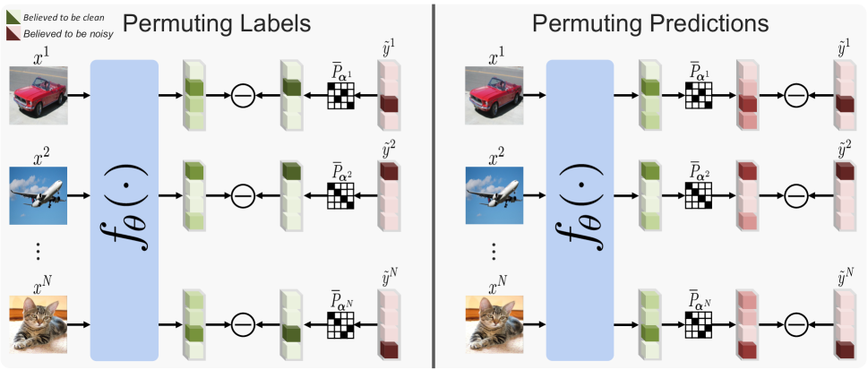
Figure 1: The diagram illustrates the two variants of integrating the permutation layer. We assume that the noisy and underlying clean labels are: $\tilde{y}^{1}=\boldsymbol{e}_{3},y^{1}=\boldsymbol{e}_{2},\tilde{y}^{2}=y^{2}=\boldsymbol{e}_{1},\tilde{y}^{N}=\boldsymbol{e}_{4},y^{N}=\boldsymbol{e}_{3}$, and that the instance-dependent permutation layers are learned successfully, i.e., $\hbox to0.0pt{\hskip 1.40451pt\leavevmode\hbox{\set@color$\overline{\hbox{}}$}\hss}{\leavevmode\hbox{\set@color$P$}}_{\!\!\boldsymbol{\alpha}^{k}}=P(\tilde{y}^{k},y^{k})$. When permuting labels, the loss is computed between the predictions and the corrected labels. However, when we instead permute the predictions, the loss is computed between the noisified predictions $P(\tilde{y}^{k},y^{k})\,f_{\theta}(x)$ and the noisy labels $\tilde{y}^{k}$. Light and dark colors represent $0$ and $1$, respectively.

3.2 Permutation Layer Integration

The proposed instance-dependent permutation layer alleviates the impact of label noise by correcting the loss. As demonstrated in Figure 1, we provide two approaches of incorporating the permutation layer into the learning procedure. Both approaches aim to capture the noise influencing $y^{k}$, i.e., $P(\tilde{y}^{k},y^{k})$. The first approach applies the permutation layer to the noisy label $\boldsymbol{e}_{\tilde{y}^{k}}$, as in equation (1). In this case, the permutation layer cleans the noisy label, $P(\tilde{y}^{k},y^{k})\,\boldsymbol{e}_{\tilde{y}^{k}}=\boldsymbol{e}_{y^{k}}$. In the second approach, we instead apply the permutation layer to the model’s prediction $f_{\theta}(\mathbf{x})$, as in equation (2). Thus, the prediction $f_{\theta}(\mathbf{x}^{k})$ is permuted to have a noise matching the noise on $y^{k}$, $P(\tilde{y}^{k},y^{k})$.

$$\pazocal{L}_{1}=\frac{1}{N}\sum_{i=1}^{N}\ell(f_{\theta}(\mathbf{x}^{i}),\,\hbox to0.0pt{\hskip 1.40451pt\leavevmode\hbox{\set@color$\overline{\hbox{}}$}\hss}{\leavevmode\hbox{\set@color$P$}}_{\!\!\boldsymbol{\alpha}^{i}}\,\boldsymbol{e}_{\tilde{y}^{i}})$$ (1)

$$\pazocal{L}_{2}=\frac{1}{N}\sum_{i=1}^{N}\ell(\hbox to0.0pt{\hskip 1.40451pt\leavevmode\hbox{\set@color$\overline{\hbox{}}$}\hss}{\leavevmode\hbox{\set@color$P$}}_{\!\!\boldsymbol{\alpha}^{i}}f_{\theta}(\mathbf{x}^{i}),\,\boldsymbol{e}_{\tilde{y}^{i}})$$ (2)

Note that these two approaches are analogues to the forward and backward corrections in (Patrini et al. 2017a). Looking closely at equation (1), we can see that it is in fact equivalent to learning the label directly. In other words minimizing $\pazocal{L}_{1}$, with respect to $\theta$ and $\{\alpha^{i}\}_{i=1}^{N}$, is equivalent to minimizing $\sum_{i}\ell(f_{\theta}(\mathbf{x}^{i}),\,S(\boldsymbol{\alpha}^{i}))$. The approach of directly learning the label was first proposed in (Tanaka et al. 2018), and then adopted by (Yi and Wu 2019). The following proposition demonstrates this equivalence by showing that applying a permutation to the label $\hbox to0.0pt{\hskip 1.40451pt\leavevmode\hbox{\set@color$\overline{\hbox{}}$}\hss}{\leavevmode\hbox{\set@color$P$}}_{\!\!\boldsymbol{\alpha}}\,\boldsymbol{e}_{\tilde{y}^{i}}$ yields $S(\boldsymbol{\alpha}^{i})$.

Proposition 1.

Given a training sample $(\mathbf{x}^{k},\tilde{y}^{k})$, we have:

$$\hbox to0.0pt{\hskip 1.40451pt\leavevmode\hbox{\set@color$\overline{\hbox{}}$}\hss}{\leavevmode\hbox{\set@color$P$}}_{\!\!\boldsymbol{\alpha}^{k}}\,\boldsymbol{e}_{\tilde{y}^{k}}=S(\boldsymbol{\alpha}^{k})$$

Proof. $\hbox to0.0pt{\hskip 1.40451pt\leavevmode\hbox{\set@color$\overline{\hbox{}}$}\hss}{\leavevmode\hbox{\set@color$P$}}_{\!\!\boldsymbol{\alpha}^{k}}\,\boldsymbol{e}_{\tilde{y}^{k}}=\sum_{i=1}^{c}S(\boldsymbol{\alpha}^{k})_{i}\,P(\tilde{y}^{k},i)\,\boldsymbol{e}_{\tilde{y}^{k}}$

$\;\;\,\,=\sum_{i=1}^{c}S(\boldsymbol{\alpha}^{k})_{i}\,\boldsymbol{e}_{i}\,=\,S(\boldsymbol{\alpha}^{k})$

∎

In the next section, we further analyze these two approaches, and analytically show that they possess different theoretical properties.

3.3 Permutation Layer Properties: Theoretical Analysis

Although the two approaches of employing the permutation layer seem equivalent, they are in fact substantially different. In this section, we compare these approaches and analytically show that applying the permutation to the prediction has two key advantages: ($i$) The optimization does not get stuck in a local optimum after solving for the permutation layer parameters $\boldsymbol{\alpha}$. ($ii$) The norm of the gradient $||\nabla_{\!\boldsymbol{\alpha}}\pazocal{L}_{2}||$ is affected by the model’s confidence, i.e., $\pazocal{L}_{2}$ is “confidence-aware”.

Getting stuck in a local minimum.

As noted by (Tanaka et al. 2018), alternating minimization of the KL-divergence loss with respect to the labels and the model parameters suffers from premature convergence to local optima. This stems from the fact that the minimum of the loss (i.e., $\pazocal{L}=0$) is attained immediately after solving with respect to the labels. In Proposition 2, we build on the observation in (Tanaka et al. 2018) and show that for any loss function satisfying assumption 1, the minimization of $\pazocal{L}_{1}$ gets stuck in a local minimum, i.e., the minimum is attained when solving for $\boldsymbol{\alpha}$. On the other hand, Proposition 3 shows that minimizing $\pazocal{L}_{2}$ does not stop prematurely, i.e., the minimum is not attained when solving for $\boldsymbol{\alpha}$.

Assumption 1.

Let $\ell(\mathbf{p},\mathbf{q}):p(c)\times p(c)\rightarrow\mathbb{R}^{+}$ , where $\,\mathbb{R}^{+}$ is the set $\{x\in\mathbb{R}|x\geq 0\}$. We assume that $\ell(\mathbf{p},\mathbf{q})=0\,$ if and only if $\,\mathbf{p}=\mathbf{q}$ .

Implications of Assumption 1.

This assumption includes most well known loss functions such as p-norm loss functions and KL-divergence. However, the cross-entropy loss generally does not satisfy this assumption (unless $\max_{i}\mathbf{q}_{i}=1$, which is the case in Proposition 3).

Proposition 2.

Let $\ell$ be a loss function satisfying assumption 1. Then, we have

$$\ell(f_{\theta}(\mathbf{x}),\hbox to0.0pt{\hskip 1.40451pt\leavevmode\hbox{\set@color$\overline{\hbox{}}$}\hss}{\leavevmode\hbox{\set@color$P$}}_{\!\!\boldsymbol{\alpha}^{\ast}(\theta)}\,\boldsymbol{e}_{\tilde{y}})=0$$

where $\boldsymbol{\alpha}^{\ast}(\theta)=\underset{\boldsymbol{\alpha}}{\arg\min}\,\ell(f_{\theta}(\mathbf{x}),\,\hbox to0.0pt{\hskip 1.40451pt\leavevmode\hbox{\set@color$\overline{\hbox{}}$}\hss}{\leavevmode\hbox{\set@color$P$}}_{\!\!\boldsymbol{\alpha}}\,\boldsymbol{e}_{\tilde{y}})$

Proof. From proposition 1, we have $\hbox to0.0pt{\hskip 1.40451pt\leavevmode\hbox{\set@color$\overline{\hbox{}}$}\hss}{\leavevmode\hbox{\set@color$P$}}_{\!\!\boldsymbol{\alpha}}\,\boldsymbol{e}_{\tilde{y}}=S(\boldsymbol{\alpha})$. Then,

$$\boldsymbol{\alpha}^{\ast}(\theta)=\underset{\boldsymbol{\alpha}}{\arg\min}\,\ell(f_{\theta}(\mathbf{x}),\,S(\boldsymbol{\alpha}))$$

$$\Rightarrow\; S\big{(}\boldsymbol{\alpha}^{\ast}(\theta)\big{)}=f_{\theta}(\mathbf{x})$$

Finally, by assumption 1 we have

$$\ell(f_{\theta}(\mathbf{x}),\hbox to0.0pt{\hskip 1.40451pt\leavevmode\hbox{\set@color$\overline{\hbox{}}$}\hss}{\leavevmode\hbox{\set@color$P$}}_{\!\!\boldsymbol{\alpha}^{\ast}(\theta)}\,\boldsymbol{e}_{\tilde{y}})=\ell(f_{\theta}(\mathbf{x}),f_{\theta}(\mathbf{x}))=0$$

∎

Proposition 3.

Let $\ell$ be a loss function satisfying assumption 1, and $\theta_{i}$ be some choice for the model’s parameter such that $\underset{j}{max}\,[f_{\theta_{i}}(\mathbf{x})]_{j}<1$. Then, we have

$$\ell(\hbox to0.0pt{\hskip 1.40451pt\leavevmode\hbox{\set@color$\overline{\hbox{}}$}\hss}{\leavevmode\hbox{\set@color$P$}}_{\!\!\boldsymbol{\alpha}^{\ast}(\theta_{i})}\,f_{\theta_{i}}(\mathbf{x}),\,\boldsymbol{e}_{\tilde{y}})>0$$

where $\boldsymbol{\alpha}^{\ast}(\theta_{i})=\underset{\boldsymbol{\alpha}}{\arg\min}\,\ell(\hbox to0.0pt{\hskip 1.40451pt\leavevmode\hbox{\set@color$\overline{\hbox{}}$}\hss}{\leavevmode\hbox{\set@color$P$}}_{\!\!\boldsymbol{\alpha}}\,f_{\theta_{i}}(\mathbf{x}),\,\boldsymbol{e}_{\tilde{y}})$

Proof. We start by showing that the two arguments of $\ell$ are not equal. It is enough to show that $\big{[}\hbox to0.0pt{\hskip 1.40451pt\leavevmode\hbox{\set@color$\overline{\hbox{}}$}\hss}{\leavevmode\hbox{\set@color$P$}}_{\!\!\boldsymbol{\alpha}^{\ast}(\theta_{i})}\,f_{\theta_{i}}(\mathbf{x})\big{]}_{\tilde{y}}<[\boldsymbol{e}_{\tilde{y}}]_{\tilde{y}}=1$.

$$\big{[}\hbox to0.0pt{\hskip 1.40451pt\leavevmode\hbox{\set@color$\overline{\hbox{}}$}\hss}{\leavevmode\hbox{\set@color$P$}}_{\!\!\boldsymbol{\alpha}^{\ast}(\theta_{i})}\,f_{\theta_{i}}(\mathbf{x})\big{]}_{\tilde{y}}=\boldsymbol{e}_{\tilde{y}}^{T}\,\hbox to0.0pt{\hskip 1.40451pt\leavevmode\hbox{\set@color$\overline{\hbox{}}$}\hss}{\leavevmode\hbox{\set@color$P$}}_{\!\!\boldsymbol{\alpha}^{\ast}(\theta_{i})}\,f_{\theta_{i}}(\mathbf{x})$$

$$=\boldsymbol{e}_{\tilde{y}}^{T}\,\sum_{j=1}^{C}S\big{(}\boldsymbol{\alpha}^{\ast}(\theta_{i})\big{)}_{j}\,P(\tilde{y},j)\,f_{\theta_{i}}(\mathbf{x})$$

$$=\sum_{j=1}^{C}S\big{(}\boldsymbol{\alpha}^{\ast}(\theta_{i})\big{)}_{j}\,\boldsymbol{e}_{j}^{T}\,f_{\theta_{i}}(\mathbf{x})$$

$$=S\big{(}\boldsymbol{\alpha}^{\ast}(\theta_{i})\big{)}^{T}\,f_{\theta_{i}}(\mathbf{x})\leq\underset{j}{\max}\,[f_{\theta_{i}}(\mathbf{x})]_{j}<1.$$

Therefore,

$$\hbox to0.0pt{\hskip 1.40451pt\leavevmode\hbox{\set@color$\overline{\hbox{}}$}\hss}{\leavevmode\hbox{\set@color$P$}}_{\!\!\boldsymbol{\alpha}^{\ast}(\theta_{i})}\,f_{\theta_{i}}(\mathbf{x})\neq\boldsymbol{e}_{\tilde{y}}$$

Finally, by assumption 1, $\,\ell(\hbox to0.0pt{\hskip 1.40451pt\leavevmode\hbox{\set@color$\overline{\hbox{}}$}\hss}{\leavevmode\hbox{\set@color$P$}}_{\!\!\boldsymbol{\alpha}^{\ast}(\theta_{i})}\,f_{\theta_{i}}(\mathbf{x}),\,\boldsymbol{e}_{\tilde{y}})>0$ ∎

Note that for classifiers with a softmax layer, i.e., $f_{\theta_{i}}(\mathbf{x})=S(h_{\theta_{i}}(\mathbf{x}))$, $\,\underset{j}{\max}\,[f_{\theta_{i}}(\mathbf{x})]_{j}<1\,$ for all $\theta_{i}$.

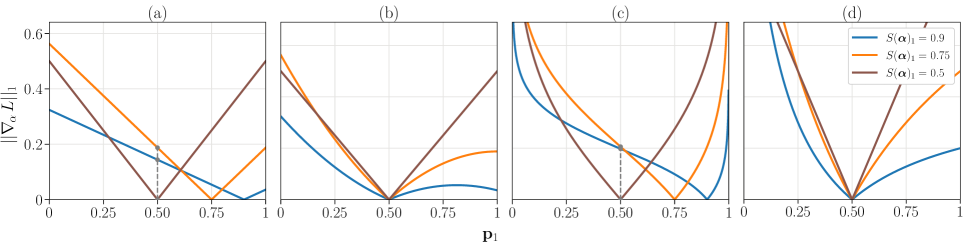
Figure 2: The relationship between $||\nabla_{\!\boldsymbol{\alpha}}L||_{1}$ and the confidence of the first class $\mathbf{p}_{1}$ over different choices of $\mathbf{\boldsymbol{\alpha}}$ and $\tilde{y}=1$. Figures (a,b) use the $L_{2}$ norm whereas (c,d) use the KL-divergence. In figures (a,c) the permutation layer is applied to the label, i.e., $L=\ell(\mathbf{p},\hbox to0.0pt{\hskip 1.40451pt\leavevmode\hbox{\set@color$\overline{\hbox{}}$}\hss}{\leavevmode\hbox{\set@color$P$}}_{\!\!\boldsymbol{\alpha}}\boldsymbol{e}_{\tilde{y}})$. In figures (b,d) the permutation is applied to the prediction, i.e., $L=\ell(\hbox to0.0pt{\hskip 1.40451pt\leavevmode\hbox{\set@color$\overline{\hbox{}}$}\hss}{\leavevmode\hbox{\set@color$P$}}_{\!\!\boldsymbol{\alpha}}\mathbf{p},\boldsymbol{e}_{\tilde{y}})$. This analysis shows that only when the permutation layer is applied to the prediction, $||\nabla_{\!\boldsymbol{\alpha}}L||_{1}$ decreases as the confidence decrease and is zero when $\mathbf{p}=[0.5,0.5]$. However, for the case of applying the permutation to the label, the gradient is zero only when $\mathbf{p}=S(\boldsymbol{\alpha})$.

Confidence-aware.

Another advantage of applying the permutation to the prediction is that the gradient norm $||\nabla_{\!\boldsymbol{\alpha}}\pazocal{L}_{2}||$ is proportional to the confidence of the classifier’s prediction, as in Proposition 4. With this approach, unconfident predictions cause minimal updates on $\boldsymbol{\alpha}$, while confident ones prompt more notable updates. We measure the confidence of a prediction $f_{\theta}(\mathbf{x})$ using $f_{\theta}(\mathbf{x})_{max}-f_{\theta}(\mathbf{x})_{min}$. We believe this behavior to be generally desirable, especially for classifiers that provide well-calibrated predictions during training (Thulasidasan et al. 2019). In well-calibrated classifiers, the predicted scores are indicative of the actual likelihood of correctness (Guo et al. 2017).

Assumption 2.

Let $\ell(\mathbf{p},\mathbf{q}):p(c)\times p(c)\rightarrow\mathbb{R}^{+}$ , where $\,\mathbb{R}^{+}$ is the set $\{x\in\mathbb{R}|x\geq 0\}$, be a loss function satisfying $||\nabla_{\!\mathbf{p}}\,\ell(\mathbf{p},\mathbf{q})||_{1}\leq M$ when $\,\mathbf{p}_{max}-\mathbf{p}_{min}<~{}1/c$ .

Where $M\in\mathbb{R}^{+}$, $\mathbf{p}$ and $\mathbf{q}$ represent the prediction and the target, respectively.

Remark on Assumption 2

This assumption is clearly satisfied for $p$-norm loss functions with $p\geq 1$. It is also satisfied for the cross-entropy loss and KL-divergence; the proof is provided in the supplementary material.

Proposition 4.

Let $\ell$ be a loss function satisfying assumption 2 and the loss for a given training sample $(\mathbf{x}^{k},\tilde{y}^{k})$ be $L=\ell(\hbox to0.0pt{\hskip 1.40451pt\leavevmode\hbox{\set@color$\overline{\hbox{}}$}\hss}{\leavevmode\hbox{\set@color$P$}}_{\!\!\boldsymbol{\alpha}^{k}}f_{\theta}(\mathbf{x}^{k}),\,\boldsymbol{e}_{\tilde{y}^{k}})$. Then, $\nabla_{\!\boldsymbol{\alpha}^{k}}L$ satisfies:

$$||\nabla_{\!\boldsymbol{\alpha}^{k}}L||_{1}\leq\frac{c\,M}{4}\big{[}f_{\theta}(\mathbf{x}^{k})_{max}-f_{\theta}(\mathbf{x}^{k})_{min}\big{]}$$

$$\text{if}\quad\big{[}f_{\theta}(\mathbf{x})_{max}-f_{\theta}(\mathbf{x})_{min}\big{]}<1/c\,.$$

where $c$ is the number of classes.

Proof. We start by taking the partial derivative of $L$ with respect to $\boldsymbol{\alpha}^{k}_{j}$, where $1\leq j\leq c$. To simplify notation, let $\tilde{f}=\hbox to0.0pt{\hskip 1.40451pt\leavevmode\hbox{\set@color$\overline{\hbox{}}$}\hss}{\leavevmode\hbox{\set@color$P$}}_{\!\!\boldsymbol{\alpha}^{k}}f_{\theta}(\mathbf{x}^{k})$

$$\Big{|}\frac{\partial L}{\partial\boldsymbol{\alpha}^{k}_{j}}\Big{|} =\Big{|}\nabla_{\!\tilde{f}}\,L\boldsymbol{\cdot}\frac{\partial\tilde{f}}{\partial\boldsymbol{\alpha}^{k}_{j}}\Big{|}$$

$$\leq\Big{|}\nabla_{\!\tilde{f}}\,L\Big{|}\boldsymbol{\cdot}\Big{|}\frac{\partial\tilde{f}}{\partial\boldsymbol{\alpha}^{k}_{j}}\Big{|}$$ (3.1)

Now, we obtain an upper bound for $\Big{|}\frac{\partial\tilde{f}}{\partial\boldsymbol{\alpha}^{k}_{j}}\Big{|}$

$$\Big{|}\frac{\partial\tilde{f}}{\partial\boldsymbol{\alpha}^{k}_{j}}\Big{|} =\Big{|}\sum_{i=1}^{c}\frac{\partial S(\boldsymbol{\alpha}^{k})_{i}}{\partial\boldsymbol{\alpha}^{k}_{j}}P(\tilde{y}^{k},i)\;f_{\theta}(\mathbf{x}^{k})\Big{|}$$

$$=\Big{|}\sum_{\begin{subarray}{c}i=1\\ i\neq j\end{subarray}}^{c}S(\boldsymbol{\alpha}^{k})_{j}S(\boldsymbol{\alpha}^{k})_{i}[P(\tilde{y}^{k},j)f_{\theta}(\mathbf{x}^{k})$$

$$\qquad\qquad\quad-P(\tilde{y}^{k},i)f_{\theta}(\mathbf{x}^{k})]\Big{|}$$

Using the triangle inequality and the fact that $\big{|}P(\tilde{y}^{k},j)f_{\theta}(\mathbf{x}^{k})-P(\tilde{y}^{k},i)f_{\theta}(\mathbf{x}^{k})\big{|}\leq\big{[}f_{\theta}(\mathbf{x}^{k})_{max}-f_{\theta}(\mathbf{x}^{k})_{min}\big{]}\,\mathbf{1}\,$, we have

$$\Big{|}\frac{\partial\tilde{f}}{\partial\boldsymbol{\alpha}^{k}_{j}}\Big{|} \leq\sum_{\begin{subarray}{c}i=1\\ i\neq j\end{subarray}}^{c}S(\boldsymbol{\alpha}^{k})_{j}S(\boldsymbol{\alpha}^{k})_{i}\big{[}f_{\theta}(\mathbf{x}^{k})_{max}-f_{\theta}(\mathbf{x}^{k})_{min}\big{]}\mathbf{1}$$

$$=S(\boldsymbol{\alpha}^{k})_{j}(1-S(\boldsymbol{\alpha}^{k})_{j})\big{[}f_{\theta}(\mathbf{x}^{k})_{max}-f_{\theta}(\mathbf{x}^{k})_{min}\big{]}\mathbf{1}$$

$$\leq\frac{1}{4}\big{[}f_{\theta}(\mathbf{x}^{k})_{max}-f_{\theta}(\mathbf{x}^{k})_{min}\big{]}\mathbf{1}$$ (3.2)

Combining $\eqref{eq:3.1}$ and $\eqref{eq:3.2}$, the partial derivative of $L$ is

$$\Big{|}\frac{\partial L}{\partial\boldsymbol{\alpha}^{k}_{j}}\Big{|} \leq\frac{1}{4}\big{[}f_{\theta}(\mathbf{x}^{k})_{max}-f_{\theta}(\mathbf{x}^{k})_{min}\big{]}\,\big{|}\big{|}\nabla_{\!\tilde{f}}\,L\big{|}\big{|}_{1}$$

By Assumption 2, we conclude that

$$||\nabla_{\!\boldsymbol{\alpha}^{k}}L||_{1} \leq\frac{c}{4}\big{[}f_{\theta}(\mathbf{x}^{k})_{max}-f_{\theta}(\mathbf{x}^{k})_{min}\big{]}\,\big{|}\big{|}\nabla_{\!\tilde{f}}\,L\big{|}\big{|}_{1}$$

$$\leq\frac{c\,M}{4}\big{[}f_{\theta}(\mathbf{x}^{k})_{max}-f_{\theta}(\mathbf{x}^{k})_{min}\big{]}$$

∎

The result in proposition 4 can be motivated intuitively by the following example.

Example:

Consider a training sample $(\mathbf{x}^{k},\tilde{y}^{k})$ where the classifier’s prediction has equal probabilities $f(\mathbf{x}^{k})=~{}\frac{1}{c}~{}\mathbf{1}$, or equivalently $f(\mathbf{x}^{k})_{max}-f(\mathbf{x}^{k})_{min}=0$. Then, it is easy to see that $\ell(\hbox to0.0pt{\hskip 1.40451pt\leavevmode\hbox{\set@color$\overline{\hbox{}}$}\hss}{\leavevmode\hbox{\set@color$P$}}_{\!\!\boldsymbol{\alpha}^{1}}f(\mathbf{x}^{k}),\,\tilde{y}^{k})=\ell(\hbox to0.0pt{\hskip 1.40451pt\leavevmode\hbox{\set@color$\overline{\hbox{}}$}\hss}{\leavevmode\hbox{\set@color$P$}}_{\!\!\boldsymbol{\alpha}^{2}}f(\mathbf{x}^{k}),\,\tilde{y}^{k})$ for all $\boldsymbol{\alpha}^{1},\boldsymbol{\alpha}^{2}\in\mathbb{R}^{c}$. This is obvious since applying the permutation layer on $\nicefrac{{1}}{{c}}~{}\mathbf{1}$ does not change its value, e.g., $\hbox to0.0pt{\hskip 1.40451pt\leavevmode\hbox{\set@color$\overline{\hbox{}}$}\hss}{\leavevmode\hbox{\set@color$P$}}_{\!\!\boldsymbol{\alpha}^{1}}\,\frac{1}{c}\,\mathbf{1}=\sum_{i=1}^{c}S(\boldsymbol{\alpha}^{1})_{i}\,P(\tilde{y}^{k},i)\,\frac{1}{c}\,\mathbf{1}=\sum_{i=1}^{c}S(\boldsymbol{\alpha}^{1})_{i}\,\frac{1}{c}\,\mathbf{1}=\frac{1}{c}\,\mathbf{1}$ Finally, we can conclude that $\nabla_{\!\boldsymbol{\alpha}}\,\ell(\hbox to0.0pt{\hskip 1.40451pt\leavevmode\hbox{\set@color$\overline{\hbox{}}$}\hss}{\leavevmode\hbox{\set@color$P$}}_{\!\!\boldsymbol{\alpha}}f(\mathbf{x}^{k}),\tilde{y}^{k})=\mathbf{0}$.

Figure 2 illustrates the confidence-aware property of $\pazocal{L}_{2}$ by plotting the relationship between $||\nabla_{\!\boldsymbol{\alpha}}L||_{1}$ and the confidence of the first class $\mathbf{p}_{1}$, in a binary classification problem. This also shows that $\pazocal{L}_{1}$ lacks this property.

3.4 Permutation Layer Learning

We simultaneously learn the model’s parameters $\theta$ and the parameters of the permutation layer $\{\boldsymbol{\alpha}^{i}\}_{i=1}^{N}$ using gradient descent. In fact, the optimization problem has a closed-form solution with respect to $\{\boldsymbol{\alpha}^{i}\}_{i=1}^{N}$. However, similar to (Yi and Wu 2019), we use gradient descent to allow for gradual changes of the parameters and to take advantage of the confidence-aware property described in proposition 4. The permutation layer parameters, $\{\boldsymbol{\alpha}^{i}\}_{i=1}^{N}$, are updated as follows:

$$\boldsymbol{\alpha}^{i}[t+1]\leftarrow\boldsymbol{\alpha}^{i}[t]-\eta_{\alpha}{}\nabla_{\!\boldsymbol{\alpha}^{i}}\pazocal{L}$$

for $1\leq i\leq N$, where $\eta_{\alpha}{}$ is the learning rate of the permutation layer. The initialization of the permutation layer weights is determined by the hyperparameter $I_{\alpha}{}$. Precisely, $I_{\alpha}{}$ affects the initialization as follows:

$$S({\boldsymbol{\alpha}}^{i})_{j}=\left\{\begin{array}[]{ll}I_{\alpha}{},&\text{if }j=\tilde{y}^{i}\\[10.00002pt] \frac{1-I_{\alpha}{}}{c-1},&\text{if }j\neq\tilde{y}^{i}\end{array}\right.,$$

where $\frac{1}{c}<I_{\alpha}{}<1$. We avoid setting $I_{\alpha}{}$ very close to 1 to allow for a more desirable gradient flow, i.e., avoiding vanishing gradients. The effects of the choices of $\eta_{\alpha}{}$ and $I_{\alpha}{}$ are analyzed in section 4.4. Note that the permutation layer is discarded at inference time.

In the previous sections, we have established the similarity between permuting the labels and Joint Optimization (Tanaka et al. 2018), and that permuting the predictions has more appealing theoretical properties. Therefore, in the next section, we empirically analyze PermLL when the permutation is applied to the prediction.

Dataset	Method	Symmetric noise				Aysmmetric noise
		20%	40%	60%	80%	20%	40%
CIFAR10	CE	86.98 ± 0.12	81.88 ± 0.29	74.14 ± 0.56	53.82 ± 1.04	88.59 ± 0.34	80.11 ± 1.44
	Bootstrap (Reed et al. 2014)	86.23 ± 0.23	82.23 ± 0.37	75.12 ± 0.56	54.12 ± 1.32	88.26 ± 0.24	81.21 ± 1.47
	Forward (Patrini et al. 2017a)	87.99 ± 0.36	83.25 ± 0.38	74.96 ± 0.65	54.64 ± 0.44	89.09 ± 0.47	83.55 ± 0.58
	GCE (Zhang and Sabuncu 2018)	89.83 ± 0.20	87.13 ± 0.22	82.54 ± 0.23	64.07 ± 1.38	89.33 ± 0.17	76.74 ± 0.61
	Joint (Tanaka et al. 2018)	92.25	90.79	86.87	69.16	-	-
	SL (Wang et al. 2019)	89.83 ± 0.32	87.13 ± 0.26	82.81 ± 0.61	68.12 ± 0.81	90.44 ± 0.27	82.51 ± 0.45
	ELR (Liu et al. 2020)	91.16 ± 0.08	89.15 ± 0.17	86.12 ± 0.49	73.86 ± 0.61	93.52 ± 0.23	90.12 ± 0.47
	SELC (Lu and He 2022)	93.09 ± 0.02	91.18 ± 0.06	87.25 ± 0.09	74.13 ± 0.14	-	91.05 ± 0.11
	PermLL	93.17 ± 0.11	91.30 ± 0.23	87.94 ± 0.21	75.83 ± 0.56	92.16 ± 0.15	86.09 ± 0.23
CIFAR100	CE	58.72 ± 0.26	48.20 ± 0.65	37.41 ± 0.94	18.10 ± 0.8	59.20 ± 0.18	42.74 ± 0.61
	Bootstrap (Reed et al. 2014)	58.27 ± 0.21	47.66 ± 0.55	34.68 ± 1.1	21.64 ± 0.97	62.14 ± 0.32	45.12 ± 0.57
	Forward (Patrini et al. 2017a)	39.19 ± 2.61	31.05 ± 1.44	19.12 ± 1.95	8.99 ± 0.58	42.46 ± 2.16	34.44 ± 1.93
	GCE (Zhang and Sabuncu 2018)	66.81 ± 0.42	61.77 ± 0.24	53.16 ± 0.78	29.16 ± 0.74	66.59 ± 0.22	47.22 ± 1.15
	Joint (Tanaka et al. 2018)	58.15	54.81	47.94	17.18	-	-
	Pencil (Yi and Wu 2019)	73.86 ± 0.34	69.12 ± 0.62	57.70 ± 3.86	fail	-	63.61 ± 0.23
	SL (Wang et al. 2019)	70.38 ± 0.13	62.27 ± 0.22	54.82 ± 0.57	25.91 ± 0.44	72.56 ± 0.22	69.32 ± 0.87
	ELR (Liu et al. 2020)	74.21 ± 0.22	68.28 ± 0.31	59.28 ± 0.67	29.78 ± 0.56	74.03 ± 0.31	73.26 ± 0.64
	SELC (Lu and He 2022)	73.63 ± 0.07	68.46 ± 0.10	59.41 ± 0.06	32.63 ± 0.06	-	70.82 ± 0.09
	PermLL	74.35 ± 0.34	71.37 ± 0.36	65.58 ± 0.37	45.81 ± 0.49	72.66 ± 0.13	51.60 ± 0.11

Table 1: Results on CIFAR10 and CIFAR100 on symmetric and asymmetric label noise with different noise levels. We report the mean and standard deviation test accuracy of our method over three random initializations. All methods use Resnet-34. Results for SL, GCE, Forward, Bootstrap are taken from (Liu et al. 2020), results from Joint are taken from (Lu and He 2022), and other results are taken from their respective papers. The best results are highlighted in bold.

Method	Result	Method	Result
CE	69.10	ELR+* (Liu et al. 2020)	74.81
Forward (Reed et al. 2014)	69.84	DivideMix* (Li, Socher, and Hoi 2020)	74.76
Pencil (Yi and Wu 2019)	73.49	UniCon* (Karim et al. 2022)	74.98
JNPL (Kim et al. 2021)	74.15	MLNT (Li et al. 2019)	73.47
Joint (Tanaka et al. 2018)	72.16	PermLL	74.99

Table 2: Test accuracy results on Clothing-1M compared to state-of-the-art methods. PermLL outperforms all other methods despite it’s simplicity. Methods denoted with * use heavy augmentations (e.g mixup), semi-supervised training and multiple networks to achieve their results

4 Experiments

4.1 Datasets

To evaluate the effectiveness of PermLL, we use three standard image classification benchmarks: CIFAR-10, CIFAR-100 (Krizhevsky, Hinton et al. 2009) and Clothing-1M (Xiao et al. 2015b). Since the CIFAR10/100 datasets are known to be clean, we simulate a noisy learning setting by injecting synthetic noise into the training labels. Two types of synthetic label noise are used: symmetric and asymmetric noise. For the symmetric noise, we take a fraction of the labels and flip them to one of the c classes with a uniform random probability. Asymmetric noise attempts to mimic the mistakes that naturally occur by annotators in the real world. We follow (Patrini et al. 2017b) for injecting the asymmetric noise in CIFAR-10: truck$\,\to\,$autombile, deer$\,\to\,$horse, bird$\,\to\,$airplane, cat $\leftrightarrow$ dog. In the case of asymmetric noise for CIFAR-100, we flip labels of subclasses within randomly selected superclasses cyclically with a total of 20 superclasses. Following (Liu et al. 2020; Tanaka et al. 2018), we hold out 10% of the training data as a validation set.

Clothing1M, on the other hand, is a large dataset of images from online clothing shops containing realistic noise. The noise level is estimated to be around 38.5% (Xiao et al. 2015b). This dataset contains four sets: a noisy training set (1M samples), a clean training set (50K samples), a clean validation set (14K samples), and a clean testing set (10K samples). In our experiments, we completely exclude the 50k samples in the clean training set as PermLL does not assume the availability of a clean training set.

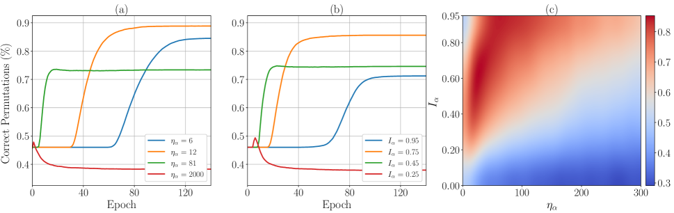
Figure 3: The effect of hyperparameter choices on the percentage of correctly learned permutation layers on CIFAR-10 with 60% symmetric noise. (a) Shows the effect of changing the permutation learning rate $\eta_{\alpha}{}$ on the percentage of correct permutations when $I_{\alpha}{}$ = 0.75. (b) Shows the effect of changing $I_{\alpha}{}$ when $\eta_{\alpha}{}$ is set to 24. (c) Shows a smoothed heatmap of the percentage of correctly learned permutations at the end of training as a function of $\eta_{\alpha}{}$ and $I_{\alpha}{}$.

4.2 Implementation

For CIFAR-10 we use a ResNet34 (He et al. 2016) and an SGD optimizer with learning rate of 0.02, momentum of 0.9, a weight decay of 0.0005 and a batch size 128. The model is trained for 120 epochs and the learning rate is decayed by a factor of 10 at epochs 80 and 100. Additionally, we apply standard augmentation and data preprocessing: padding followed by random cropping, random horizontal flip, and data normalization, similar to (Liu et al. 2020; Tanaka et al. 2018; Yi and Wu 2019). The same setup is used for CIFAR-100 except that the weight decay used is 0.001, and the learning rate decays once by a factor of 10 at epoch 100. For all noise settings in CIFAR10 we set $I_{\alpha}{}=0.35$, and $\eta_{\alpha}{}=1.5$. For CIFAR100 we use $I_{\alpha}{}=0.225$, with $\eta_{\alpha}{}=3$ for symmetric noise and $\eta_{\alpha}{}=6$ for asymmetric noise.

For Clothing1M we use a pretrained Resnet50 from TorchVision (Paszke et al. 2019) and an SGD optimizer with learning rate of 0.001, momentum of 0.9, a weight decay of 0.001, and a batch size of 64. The model is trained for 15 epochs and the learning rate is decayed by a factor of 10 at epochs 5, 10 and 13, with $I_{\alpha}{}=0.275$ and $\eta_{\alpha}{}=80$. Standard augmentation and data preprocessing are applied; the images are normalized, resized to 256x256, randomly cropped to 224x224, and randomly horizontally flipped. Similar to previous methods (Liu et al. 2020; Li, Socher, and Hoi 2020), during training, we sample balanced batches (based on the noisy labels) as Clothing1M contains significant class imbalance. All experiments were implemented using PyTorch (Paszke et al. 2019) and were run on NVIDIA V100 and NVIDIA RTX A6000 GPUs.

4.3 Results

Table 1 shows the results of PermLL on CIFAR10/100 with symmetric and asymmetric synthetic noise. We compare our results with state-of-the-art methods that use a similar setup (e.g., same architecture and augmentation). To ensure fairness, we use the same architecture, batch size, and augmentation as other baselines when possible (as described in 4.2). PermLL consistently outperforms all other methods in symmetric noise. This is especially clear in the high noise CIFAR100 setting, in which PermLL achieves an improvement of $\sim$6% and $\sim$12% in terms of test accuracy for 60% and 80% symmetric noise, respectively, while using the same hyperparameters for all noise percentages. In the case of simulated asymmetric noise, our method attains comparable performance at 20% noise. In the 40% simulated asymmetric noise, our method achieves poor performance compared to the baselines. However, we observe that PermLL does not face the same issue when faced with real asymmetric instance-dependent noise.

To validate the efficacy of PermLL in real noise environments, we use the Clothing-1M dataset as a benchmark. We report the test accuracy in Table 2 of PermLL and compare it with state-of-the-art methods. We achieve high performance and outperform all baselines, slightly outperforming UniCon. It is worth noting that the comparison might not be entirely fair as methods denoted with (*), unlike PermLL, use semi-supervised training, heavy augmentation, and multiple networks to achieve their results. Nevertheless, PermLL remarkably achieves very competitive results despite its relative simplicity, demonstrating its practicality and strength.

4.4 Hyperparameter Analysis

In this section, we analyze the effect of PermLL hyperparameters on learning correct permutation layers, similar to (Tanaka et al. 2018; Yi and Wu 2019). Recall that, we ultimately want to learn $\boldsymbol{\alpha}^{i}$ such that $\hbox to0.0pt{\hskip 1.40451pt\leavevmode\hbox{\set@color$\overline{\hbox{}}$}\hss}{\leavevmode\hbox{\set@color$P$}}_{\!\!\boldsymbol{\alpha}^{i}}=P(\tilde{y}^{i},y^{i})$ for all $i$, where $\tilde{y}^{i}$ and $y^{i}$ are the clean and noisy labels, respectively. Therefore, we consider a permutation layer to be correct if $\arg\max_{j}\boldsymbol{\alpha}^{i}_{j}=y^{i}$ for all $i$.

Figure 3 (a) shows the impact of changing the permutation layer’s learning rate $\eta_{\alpha}{}$ on the percentage of correct permutations throughout training. A small $\eta_{\alpha}{}$ delays or halts learning the permutation layers, causing the model to memorize the noisy labels. In contrast, a large $\eta_{\alpha}{}$ results in early and erroneous permutations. Furthermore, an extremely large $\eta_{\alpha}{}$ reduces the percentage of correct permutations below its initial value, as early wrong predictions cause harmful large updates on the permutation layer parameters. Similarly in Figure 3 (b), we study the effect of changing $I_{\alpha}{}$. The effect appears to be inversely similar to the effect of changing $\eta_{\alpha}{}$. Analogous to the case of a high $\eta_{\alpha}{}$, extremely small $I_{\alpha}{}$ significantly reduces the permutation accuracy. Figure 3 (c) illustrates the relationship between $I_{\alpha}{}$ and $\eta_{\alpha}{}$, showing their influence on the percentage of correct permutations over a larger scale. The percentage of correct permutations suffers the most when $I_{\alpha}{}$ is low and $\eta_{\alpha}{}$ is high. We can also notice that as we increase $\eta_{\alpha}{}$ we also need to increase $I_{\alpha}{}$ to maintain a good permutation accuracy.

5 Conclusion

We proposed PermLL, a loss correction framework for learning from noisy labels. PermLL generalizes the idea of learning the labels directly, proposed in previous methods, by using instance-dependent permutation layers that can be applied to either the labels or the predictions. We theoretically investigated the differences between the two approaches and demonstrated that applying the permutation layer to the predictions has advantageous properties. Additionally, we experimentally validated the effectiveness of PermLL on synthetic and real datasets by achieving state-of-the-art performance. Finally, we analyzed the effect of adjusting the hyperparameters of PermLL on the percentage of correctly learned permutation layers.

References

- Arazo et al. (2019) Arazo, E.; Ortego, D.; Albert, P.; O’Connor, N.; and McGuinness, K. 2019. Unsupervised label noise modeling and loss correction. In International conference on machine learning, 312–321. PMLR.
- Chen and Gupta (2015) Chen, X.; and Gupta, A. 2015. Webly supervised learning of convolutional networks. In Proceedings of the IEEE international conference on computer vision, 1431–1439.
- Farabet et al. (2012) Farabet, C.; Couprie, C.; Najman, L.; and LeCun, Y. 2012. Learning hierarchical features for scene labeling. IEEE transactions on pattern analysis and machine intelligence, 35: 1915–1929.
- Frénay and Verleysen (2013) Frénay, B.; and Verleysen, M. 2013. Classification in the presence of label noise: a survey. IEEE transactions on neural networks and learning systems, 25: 845–869.
- Guo et al. (2017) Guo, C.; Pleiss, G.; Sun, Y.; and Weinberger, K. Q. 2017. On calibration of modern neural networks. In International conference on machine learning, 1321–1330. PMLR.
- Han et al. (2018) Han, B.; Yao, Q.; Yu, X.; Niu, G.; Xu, M.; Hu, W.; Tsang, I.; and Sugiyama, M. 2018. Co-teaching: Robust training of deep neural networks with extremely noisy labels. Advances in neural information processing systems, 31.
- He et al. (2016) He, K.; Zhang, X.; Ren, S.; and Sun, J. 2016. Deep residual learning for image recognition. In Proceedings of the IEEE conference on computer vision and pattern recognition, 770–778.
- Hendrycks et al. (2018) Hendrycks, D.; Mazeika, M.; Wilson, D.; and Gimpel, K. 2018. Using trusted data to train deep networks on labels corrupted by severe noise. Advances in neural information processing systems, 31.
- Karim et al. (2022) Karim, N.; Rizve, M. N.; Rahnavard, N.; Mian, A.; and Shah, M. 2022. UNICON: Combating Label Noise Through Uniform Selection and Contrastive Learning. In Proceedings of the IEEE/CVF Conference on Computer Vision and Pattern Recognition, 9676–9686.
- Kim et al. (2021) Kim, Y.; Yun, J.; Shon, H.; and Kim, J. 2021. Joint negative and positive learning for noisy labels. In Proceedings of the IEEE/CVF Conference on Computer Vision and Pattern Recognition, 9442–9451.
- Krizhevsky, Hinton et al. (2009) Krizhevsky, A.; Hinton, G.; et al. 2009. Learning multiple layers of features from tiny images.
- Krizhevsky, Sutskever, and Hinton (2012) Krizhevsky, A.; Sutskever, I.; and Hinton, G. E. 2012. Imagenet classification with deep convolutional neural networks. Advances in neural information processing systems, 25.
- Lee et al. (2018) Lee, K.-H.; He, X.; Zhang, L.; and Yang, L. 2018. Cleannet: Transfer learning for scalable image classifier training with label noise. In Proceedings of the IEEE conference on computer vision and pattern recognition, 5447–5456.
- Li, Socher, and Hoi (2020) Li, J.; Socher, R.; and Hoi, S. C. 2020. Dividemix: Learning with noisy labels as semi-supervised learning. arXiv preprint arXiv:2002.07394.
- Li et al. (2019) Li, J.; Wong, Y.; Zhao, Q.; and Kankanhalli, M. S. 2019. Learning to learn from noisy labeled data. In Proceedings of the IEEE/CVF Conference on Computer Vision and Pattern Recognition, 5051–5059.
- Liu et al. (2020) Liu, S.; Niles-Weed, J.; Razavian, N.; and Fernandez-Granda, C. 2020. Early-Learning Regularization Prevents Memorization of Noisy Labels. Advances in Neural Information Processing Systems, 33.
- Lloyd et al. (2004) Lloyd, R. V.; Erickson, L. A.; Casey, M. B.; Lam, K. Y.; Lohse, C. M.; Asa, S. L.; Chan, J. K.; DeLellis, R. A.; Harach, H. R.; Kakudo, K.; et al. 2004. Observer variation in the diagnosis of follicular variant of papillary thyroid carcinoma. The American journal of surgical pathology, 28: 1336–1340.
- Long, Shelhamer, and Darrell (2015) Long, J.; Shelhamer, E.; and Darrell, T. 2015. Fully convolutional networks for semantic segmentation. In Proceedings of the IEEE conference on computer vision and pattern recognition, 3431–3440.
- Lu and He (2022) Lu, Y.; and He, W. 2022. SELC: Self-Ensemble Label Correction Improves Learning with Noisy Labels. In Raedt, L. D., ed., Proceedings of the Thirty-First International Joint Conference on Artificial Intelligence, IJCAI-22, 3278–3284. International Joint Conferences on Artificial Intelligence Organization. Main Track.
- Maennel et al. (2020) Maennel, H.; Alabdulmohsin, I. M.; Tolstikhin, I. O.; Baldock, R.; Bousquet, O.; Gelly, S.; and Keysers, D. 2020. What do neural networks learn when trained with random labels? Advances in Neural Information Processing Systems, 33: 19693–19704.
- Malach and Shalev-Shwartz (2017) Malach, E.; and Shalev-Shwartz, S. 2017. Decoupling” when to update” from” how to update”. Advances in neural information processing systems, 30.
- Natarajan et al. (2013) Natarajan, N.; Dhillon, I. S.; Ravikumar, P. K.; and Tewari, A. 2013. Learning with noisy labels. Advances in neural information processing systems, 26.
- Paolacci, Chandler, and Ipeirotis (2010) Paolacci, G.; Chandler, J.; and Ipeirotis, P. G. 2010. Running experiments on amazon mechanical turk. Judgment and Decision making, 5: 411–419.
- Paszke et al. (2019) Paszke, A.; Gross, S.; Massa, F.; Lerer, A.; Bradbury, J.; Chanan, G.; Killeen, T.; Lin, Z.; Gimelshein, N.; Antiga, L.; Desmaison, A.; Kopf, A.; Yang, E.; DeVito, Z.; Raison, M.; Tejani, A.; Chilamkurthy, S.; Steiner, B.; Fang, L.; Bai, J.; and Chintala, S. 2019. PyTorch: An Imperative Style, High-Performance Deep Learning Library. In Wallach, H.; Larochelle, H.; Beygelzimer, A.; d'Alché-Buc, F.; Fox, E.; and Garnett, R., eds., Advances in Neural Information Processing Systems 32, 8024–8035. Curran Associates, Inc.
- Patrini et al. (2017a) Patrini, G.; Rozza, A.; Krishna Menon, A.; Nock, R.; and Qu, L. 2017a. Making deep neural networks robust to label noise: A loss correction approach. In Proceedings of the IEEE conference on computer vision and pattern recognition, 1944–1952.
- Patrini et al. (2017b) Patrini, G.; Rozza, A.; Krishna Menon, A.; Nock, R.; and Qu, L. 2017b. Making Deep Neural Networks Robust to Label Noise: A Loss Correction Approach. In Proceedings of the IEEE Conference on Computer Vision and Pattern Recognition (CVPR).
- Redmon et al. (2016) Redmon, J.; Divvala, S.; Girshick, R.; and Farhadi, A. 2016. You only look once: Unified, real-time object detection. In Proceedings of the IEEE conference on computer vision and pattern recognition, 779–788.
- Reed et al. (2014) Reed, S.; Lee, H.; Anguelov, D.; Szegedy, C.; Erhan, D.; and Rabinovich, A. 2014. Training deep neural networks on noisy labels with bootstrapping. arXiv preprint arXiv:1412.6596.
- Scott, Blanchard, and Handy (2013) Scott, C.; Blanchard, G.; and Handy, G. 2013. Classification with asymmetric label noise: Consistency and maximal denoising. In Conference on learning theory, 489–511.
- Song et al. (2021) Song, H.; Kim, M.; Park, D.; Shin, Y.; and Lee, J.-G. 2021. Robust learning by self-transition for handling noisy labels. In Proceedings of the 27th ACM SIGKDD Conference on Knowledge Discovery & Data Mining, 1490–1500.
- Song et al. (2022) Song, H.; Kim, M.; Park, D.; Shin, Y.; and Lee, J.-G. 2022. Learning from noisy labels with deep neural networks: A survey. IEEE Transactions on Neural Networks and Learning Systems.
- Sukhbaatar et al. (2014) Sukhbaatar, S.; Bruna, J.; Paluri, M.; Bourdev, L.; and Fergus, R. 2014. Training convolutional networks with noisy labels. arXiv preprint arXiv:1406.2080.
- Tanaka et al. (2018) Tanaka, D.; Ikami, D.; Yamasaki, T.; and Aizawa, K. 2018. Joint optimization framework for learning with noisy labels. In Proceedings of the IEEE conference on computer vision and pattern recognition, 5552–5560.
- Thulasidasan et al. (2019) Thulasidasan, S.; Chennupati, G.; Bilmes, J. A.; Bhattacharya, T.; and Michalak, S. 2019. On mixup training: Improved calibration and predictive uncertainty for deep neural networks. Advances in Neural Information Processing Systems, 32.
- Wang et al. (2019) Wang, Y.; Ma, X.; Chen, Z.; Luo, Y.; Yi, J.; and Bailey, J. 2019. Symmetric cross entropy for robust learning with noisy labels. In Proceedings of the IEEE/CVF International Conference on Computer Vision, 322–330.
- Xia et al. (2019) Xia, X.; Liu, T.; Wang, N.; Han, B.; Gong, C.; Niu, G.; and Sugiyama, M. 2019. Are anchor points really indispensable in label-noise learning? Advances in Neural Information Processing Systems, 32.
- Xiao et al. (2015a) Xiao, T.; Xia, T.; Yang, Y.; Huang, C.; and Wang, X. 2015a. Learning from massive noisy labeled data for image classification. In Proceedings of the IEEE conference on computer vision and pattern recognition, 2691–2699.
- Xiao et al. (2015b) Xiao, T.; Xia, T.; Yang, Y.; Huang, C.; and Wang, X. 2015b. Learning from massive noisy labeled data for image classification. In Proceedings of the IEEE conference on computer vision and pattern recognition, 2691–2699.
- Yao et al. (2020) Yao, Y.; Liu, T.; Han, B.; Gong, M.; Deng, J.; Niu, G.; and Sugiyama, M. 2020. Dual t: Reducing estimation error for transition matrix in label-noise learning. Advances in neural information processing systems, 33: 7260–7271.
- Yi and Wu (2019) Yi, K.; and Wu, J. 2019. Probabilistic end-to-end noise correction for learning with noisy labels. In Proceedings of the IEEE/CVF Conference on Computer Vision and Pattern Recognition, 7017–7025.
- Yu et al. (2019) Yu, X.; Han, B.; Yao, J.; Niu, G.; Tsang, I.; and Sugiyama, M. 2019. How does disagreement help generalization against label corruption? In International Conference on Machine Learning, 7164–7173. PMLR.
- Zhang et al. (2021) Zhang, C.; Bengio, S.; Hardt, M.; Recht, B.; and Vinyals, O. 2021. Understanding deep learning (still) requires rethinking generalization. Communications of the ACM, 64: 107–115.
- Zhang and Sabuncu (2018) Zhang, Z.; and Sabuncu, M. 2018. Generalized cross entropy loss for training deep neural networks with noisy labels. Advances in neural information processing systems, 31.