Yukawa Friedel-Tail pair potentials for warm dense matter applications

Abstract

Accurate equations of state (EOS) and plasma transport properties are essential for numerical simulations of warm dense matter encountered in many high-energy-density situations. Molecular dynamics (MD) is a simulation method that generates EOS and transport data using an externally provided potential to dynamically evolve the particles without further reference to the electrons. To minimize computational cost, pair potentials needed in MD may be obtained from the neutral-pseudoatom (NPA) approach, a form of single-ion density functional theory (DFT), where many-ion effects are included via ion-ion correlation functionals. Standard $N$-ion DFT-MD provides pair potentials via the force matching technique but at much greater computational cost. Here we propose a simple analytic model for pair potentials with physically meaningful parameters based on a Yukawa form with a thermally damped Friedel tail (YFT) applicable to systems containing free electrons. The YFT model accurately fits NPA pair potentials or the non-parametric force-matched potentials from $N$-ion DFT-MD, showing excellent agreement for a wide range of conditions. The YFT form provides accurate extrapolations of the NPA or force-matched potentials for small and large particle separations within a physical model. Our method can be adopted to treat plasma mixtures, allowing for large-scale simulations of multi-species warm dense matter.

I Introduction

Studies in warm dense matter (WDM) systems straddle an intermediate regime of matter extending from cold solids to hot plasmas, at arbitrary compressions and states of ionization GaffneyHDP18 ; Grabowski20 ; Hungary16 ; cdw-cpp15 ; NgIJQC12 . The ions are usually modeled as classical particles whereas the electrons are treated quantum mechanically stanton2018multiscale . Typical WDM systems often fall into regimes of average mass density $\bar{\rho}$ and temperature $T$ where reliable experimental data do not exist or are not easily available, as in most astrophysical and geophysical applications. The same issue arises in high-energy-density applications where energy is deposited in femto-second time-scales producing systems containing multi-species quasi-equilibria associated with multiple temperatures NgIJQC12 ; CDW-cm-91 ; ELR98 . The electrons and holes in semi-conductor nanostructures also behave like WDM systems due to the small effective masses of the charge carriers lfc1-dw19 . The electronic and ionic interactions in these finite-temperature systems are such that interparticle effects are strong; hence simple models of the effective pair potential fail when applied to such many-particle systems Stanek21 .

Furthermore, the equations of state (EOS) GaffneyHDP18 and transport properties  Grabowski20 of WDM systems require the tabulation of many data points and the available many-body quantum techniques, e.g., density functional theory (DFT), path-integral Monte Carlo (PIMC) methods etc., become computationally expensive. Here we aim to leverage results of DFT based $N$-ion simulation codes VASP ; ABINIT to (i) validate the functional form of physically motivated models to represent pair interactions, and (ii) elucidate the regions of physical space for which simpler models are valid. Using validated pair potentials, we avoid carrying out repeated (“on-the-fly”) $N$-ion DFT calculations as the ion system is evolved using “classical molecular dynamics”. Here, “classical molecular dynamics” implies that the electronic structure calculation needed for ion interactions is pre-computed. We emphasize that this pair potential description does not neglect many-ion effects as explained below. The relationship between the pair energy and the pair potential, and how higher-order corrections are included, are considered in Sec. VII. The standard DFT-MD procedure that determines the electronic structure of an $N$-atom sample of the material via Kohn-Sham-Mermin finite-temperature DFT (e.g., as available in computational packages VASP ; ABINIT ), together with the use of classical MD to evolve the ions to equilibrium will be referred to here as “QMD” for brevity.

The computational cost associated with $N$-ion DFT can be reduced by using a single-ion DFT approach DWP82 ; eos95 ; Hungary16 ; cdw-pop21 where an ion-ion exchange-correlation (XC) functional is used to reduce the many-ion problem to that of a single ion such that the material is a simple superposition of pseudoatoms. This does not mean that a simple superposition of actual atoms is used, as may be possible in weakly coupled systems. This “single-ion” DFT approach to the many-ion, many-electron problem is referred to here as the neutral-pseudoatom (NPA) model. The NPA calculations, being similar to average-atom (AA) calculations, are computationally rapid in comparison to QMD calculations, and usually produce EOS data and pair potentials that are in good agreement with QMD results Stanek21 ; cdwSi20 ; Hungary16 . The NPA calculations also directly yield single-ion properties like the mean-value of the charge ($\bar{Z}$) carried by ions, electron-ion scattering cross sections, or electron-ion pseudopotentials that are useful for transport calculations Grabowski20 . Note that there are many AA models SternZbar07 ; Rosznyai08 ; FausAA10 ; Murillo13 ; StaSau13 ; StaSau16 that are similar in spirit but differ in their details. Examples include different choices of functionals used to treat exchange-correlation and kinetic energy, and more significantly, the boundary conditions used in defining the AA which may be confined to a Wigner-Seitz sphere or to a much larger volume DWP82 . The particular NPA model used here is described in detail in Refs. cdwSi20 ; cdw-Carbon10E6-21 ; eos95 and will be referred to here generically as “NPA.”

Recently, machine learning (ML) methods have been employed to accelerate the calculation of multi-center interatomic potentials (MCPs) whose simplest member is the pair potential. One of the simplest ML methods is force matching ercolessi1994interatomic which aims to minimize a loss function constructed from interionic forces from a QMD dataset and a predetermined force law Stanek21 ; Brommer2007Potfit ; Brommer2006Potfit ; Brommer2015Potfit . Such a loss function may take the form

$$L(\xi)=\sum_{k=1}^{3M}w_{k}^{F}(F_{k}(\xi)-F_{k}^{0})^{2} +\sum_{\ell=1}^{M}w_{\ell}^{E}(E_{\ell}(\xi)-E_{\ell}^{0})^{2}$$

$$+\sum_{m=1}^{6M}w_{m}^{S}(S_{m}(\xi)-S_{m}^{0})^{2},$$ (1)

where $M$ denotes the number of particle coordinate configurations, $F_{k}(\xi),E_{\ell}(\xi)$, and $S_{m}(\xi)$ are the force component, energy, and stress tensor component from the target interaction potential parametrized by $\xi$ with weights $w_{k}^{F},w_{\ell}^{E},$ and $w_{m}^{S}$. The reference force component, energy, and stress component, $F^{0}_{k},E^{0}_{\ell}$, and $S^{0}_{m}$, are determined from high-fidelity calculations such as Kohn-Sham DFT MD. The last two terms in Eq. (1) can be thought of as regularizers of the loss function that restrict the functional from of the optimized interaction potential. In the following, all of our force-matched (FM) potentials assume a loss function given by Eq. (1) with $w_{\ell}^{E}=w_{m}^{S}=0$. More advanced machine learning approaches allow for greater than pair or three-body interactions by including density-density correlations thompson2015spectral . Deep neural networks have also been employed to learn the QMD potential energy surface where translational, rotational, and permutational symmetries are enforced zhang2018deep ; DeepLearning-QZeng21 . In all of the aforementioned ML methods the MCP is obtained for use in classical MD simulations. In the MCP approach the electron sub-system is suppressed, and hence higher-order (e.g, 3-body, 4-body) potentials are needed to capture the electronic energies that are not explicitly included; the philosophy is similar to that of the classic Stillinger-Weber potentials SW85 .

In contrast, the NPA approach uses only pair potentials, but explicitly includes electron contributions to the total free energy directly available from the NPA calculation, as indicated in more detail in Sec. VII. The NPA uses the electron density to calculate energy contributions from the electron subsystem whereas the MCP method tries to embody them in the MCPs that carry “electronic bonding information.” This is claimed to allow the MCP method to deal with structural defects (e.g., dislocations in metals) “on the fly,” without resorting to explicitly handling electronic effects arising from such inhomogeneities. There is however no underlying principle in physics which asserts that there exists a general classical MCP that determines the physics of general electron-ions systems in the way claimed by ML; the only available principle, due to Hohenberg and Kohn, is that there exists a one-body density functional that is universal.

An advantage of ML methods is that the functional form of the ion-ion pair interaction potential is allowed to be determined by data, eliminating any bias associated with assuming too simple a functional form based on a limited physical model. On the other hand, the lack of a functional form prevents accurate recovery of asymptotic forms imposed by the physics of these systems. The data-driven nature of these ML methods is also one of their main limitations: the pair interaction potential will only be as accurate as the data used in the training process. It is possible that the QMD dataset may consist of too few time steps, resulting in a poor representation of the potential energy surface. The QMD dataset may also contain errors that originate from simulations of a small number of particles (referred to herein as finite-size effects). Quantifying errors from finite-size effects is critically important near phase transitions where the cooperative effect of a large number of particles occurs.

Furthermore, as very complex $N$-atom structures become possible with large-$N$ simulations, increasingly more advanced XC functionals become imperative. It has been shown that numerical results using different XC functionals at different levels of the “Jacob’s ladder” may give significantly different results in such calculations Remsing17 .

To mitigate the concerns associated with dataset inadequacies, we present a parametrized analytic form of a pair potential based on a general physical model that is found to be able to fit either to potentials extracted from QMD simulations or given by NPA calculations. If the QMD dataset is expected to be comprehensive enough to describe the potential energy surface, the analytic fit form will correct for finite-size effects at both small and large interatomic distances.

We note that the NPA is a DFT method where both the electron many-body problem and the ion many-body problem are jointly reduced to equivalent non-interacting one-body problems. This is done by relegating higher-order effects beyond mean-fields into exchange-correlation (XC) functionals; these depend only on the electron one-body density and the ion one-body density. Since a central ion is used as the origin of the NPA calculation, the one-body ion-density becomes effectively a two-body ion density and correlations beyond the two-body potential appear in the ion-ion XC-correlation functionals; classical ions have no exchange, and the correlations used in the NPA for solids, liquids, or hot plasmas are those brought in by the Ornstein-Zernike procedure. Thus, while the ion-ion XC-functional is strongly non-local, the electron-electron XC-functional used in the NPA is the finite-$T$ functional given by Perrot and Dharma-wardana PDWXC , within the local-density approximation. Due to the simplicity of the electron density profile in the NPA (which is a single-center screened ion), the local-density approximation is found to be sufficient.

In the following we treat simple fluids like liquid Al as well as complex liquids like liquid C, not only at high temperatures, but also at low temperatures where the static structure factors $S(k)$ and pair-distribution functions (PDFs) $g(r)$ may be thought to depend on bond-angle distributions and other complex correlation effects. However, density functional theory is a theory of the ground state energy for systems at $T=0$ and a theory of the free energy for finite-$T$ systems. These depend only on the time-averaged picture of the fluid which is uniform as we are not treating nanostructures or solids. Hence there is no need to include the detailed instantaneous bond-orientational details that are generated in standard $N$-ion simulations, only to be averaged out using millions of such calculations. The static (i.e., long-time average) correlations beyond the two-body terms are brought into the NPA calculations via the Ornstein-Zernike procedure which requires the use of an ion-ion XC functional, as shown in Ref. DWP82 . The energy effect of such correlations is taken care of in the NPA through the ion-ion XC functionals, as discussed in Ref. DWP82 . Furthermore, the energy and free energy are functionals of just the static one-body densities. Unlike in $N$-ion DFT simulations, calculations using the NPA method will not yield instantaneous bonding details and “snap shots” of the fluid, although the static PDFs and static structure factors become readily available. However, as shown by Hafner Hafner89 for liquid As, a simple pair potential can be used to provide considerable information on bond-angle distributions by using the pair potential in a classical simulation.

In this study, we focus on the pair potentials obtained from the NPA model, and on force-matched potentials extracted from QMD where they are available. They are of interest for simulating physical systems such as liquid metals, WDM systems, and strongly coupled plasmas where the primary input to classical MD simulations is the pair potential cdw-aers83 ; chenlai92 ; Utah12 ; VorbGeri-Pots13 ; whitley15 ; Stanek21 . Specifically, we use the NPA model to generate pseudopotentials and pair potentials needed for computations of physical properties of finite-temperature electron-ion systems of uniform density, and show that a simple physically meaningful parametrization of the potentials exists for them. The simplest method, based on a linear-response approach to the pseudopotentials, is found to be applicable for a wide range of densities and temperatures. Examples where linear-response fails are common for expanded metals, liquid (which we denote as $l$-) C, and $l$-transition metals at low $\bar{\rho}$ and $T$ Stanek21 . In such cases special procedures and sophisticated XC-functionals are needed, even in standard $N$-atom DFT.

In this study, we provide pair potentials for simple fluids like $l$-Al and complex fluids like $l$-C whose QMD simulations show the existence of transient covalent bonds. Nevertheless, it was shown in detail that a simple-metal model is applicable to the thermodynamic and structural properties of $l$-C and $l$-Si, and even to their phase transitions cdw-carb22 ; cdwSi20 . These results may seem to go against “chemical intuition” but are consistent with well established physics-based insights on the ionic correlations in simple and complex liquid metals and solids Hafner87 .

The remainder of this manuscript is organized as follows. First, in Sec. II, we present a brief overview of the NPA model and pair potentials. We discuss the theory of NPA pseudopotentials which originates from the Kohn-Sham DFT electron density. We also describe how pair potentials stem from linear-response theory and their implementation in the NPA model. The NPA pair potentials are shown to agree closely with force-matched QMD pair potentials which are available for length scales limited to the size of the simulation box used in QMD. Then, in Sec. III, we introduce a simple but generally applicable parametrization scheme for pair potentials in homogeneous metallic systems. The proposed parametrization is consistent with a simple physical picture based on screened Coulomb interactions of the Yukawa type, and includes thermally damped Friedel oscillations as they become long-ranged and important for $T<E_{F}$. In Secs. IV to VI we present fits to our parametrization scheme using pair-potentials from NPA calculations for $l$-C, $l$-Al, and $l$-Li. We show that our parametrized scheme accurately reproduces structural quantities obtained from QMD or PIMC calculations and can be used to greatly reduce errors incurred from finite-size effects in QMD simulations.

II The NPA pseudopotentials and pair potentials

The NPA calculation self-consistently generates the Kohn-Sham one-body electron density distribution $n(r)$ around a nucleus placed in the appropriate environment in the fluid where an all-electron calculation is used. For simplicity of exposition here we consider the case where the bound electrons are well localized inside the Wigner-Seitz sphere of radius $r_{\rm ws}$ associated with the ion. Then, the electron distribution can be unambiguously written as a sum of a bound electron part denoted as $n_{b}(r)$ and a free electron part denoted as $n_{f}(r)$, while the issues arising from the more general case are discussed in Appendix A. The free electrons are not confined to the Wigner-Seitz sphere (as in many AA models), and occupy the whole of space represented by a large “correlation sphere” of radius $R_{c}$ which is some five to ten times $r_{\rm ws}$, chosen to ensure that all interparticle correlations are sufficiently small by $r=R_{c}$, i.e, all pair distribution functions (PDFs) $g(r)\to 1$ as $r\to R_{c}$. The electron chemical potential is the non-interacting value used in DFT and need not be re-assigned as in many AA models that use a Wigner-Seitz sphere to define and AA. The free-electron density $n_{f}(r)$ is used to construct a pseudopotential which is then employed to construct a pair potential. If a metallic model with strong screening is assumed, the above steps can be carried out within linear-response theory, giving rise to simple local (i.e., $s$-wave) pseudopotentials that contrast with the non-local non-linear pseudopotentials supplied with QMD codes VASP ; ABINIT .

At the end of an NPA calculation we have the free-electron density distribution $n_{f}(r)$ around the ion of mean charge $\bar{Z}$, where the average (uniform) free-electron density $\bar{n}=\bar{Z}\bar{\rho}$ as required by charge neutrality. The evaluation of $\bar{Z}$ used in the NPA is both an atomic physics calculation and a thermodynamic ionization-balance calculation that satisfies the Friedel sum rule and charge neutrality.

II.1 The pseudopotential

Finite-$T$ pseudopotentials based on NPA-type models were first used by Dharma-wardana and Perrot DWP-carb90 and Perrot Perrot90 , following the zero-$T$ analogues used in the physics of metals. The pseudopotential is the potential exerted by the unscreened ion of charge $\bar{Z}$ made up of the nucleus plus its core-electrons. The direct output of the NPA calculation is the full non-linear response of the electron fluid to the central nucleus together with the ion distribution whose $g(r)$ is modeled by a simple spherical cavity of radius $r_{\rm ws}$. The latter has been self-consistently adjusted to satisfy the NPA equations, as described in Ref. cdwSi20 . Then, the free-electron pileup $\Delta n_{f}(r)$ caused purely by the nucleus and its bound core is obtained by correcting for the effect of the $g(r)$ modeled as a cavity according to the method discussed in Refs. cdwSi20 and eos95 . That is, we use the cavity-corrected free-electron charge pileup $\Delta n_{f}(r)=n_{f}(r)-\bar{n}$ and its Fourier transform $\Delta n_{f}(k)$ to construct the electron-ion pseudopotential (in Hartree atomic units),

$$U_{ei}(k) = \Delta n_{f}(k)/\chi(k,r_{\rm{s}},T)$$ (2)

$$\equiv -\bar{Z}V_{k}M_{k}.$$

The negative sign in the second equation arises from the electron chagre $e=-1$. Here $V_{k}=4\pi/k^{2}$ and $\chi(k,r_{\rm{s}},T)$, which we abbreviate as $\chi(k)$, is the fully interacting finite-temperature response function of the uniform electron fluid at the density $\bar{n}$ associated with the electron Wigner-Seitz radius $r_{\rm{s}}$. The behavior of the screening function heavily depends on the degeneracy parameter $\theta=T/E_{F}$ where $E_{F}$ is the Fermi energy. The details of the calculation of $\chi(k)$ as well as the limitations of this pseudopotential are discussed in Refs. Stanek21 ; cdw-pop21 . Here we note that an all-electron non-linear DFT calculation has been applied to the electron-nuclear interaction in obtaining $\Delta n_{f}(r)$, and linear response is used only in defining a pseudopotential. Thus the pseudopotential incorporates the non-linear aspects of the Kohn-Sham calculation.

The domain of validity of the method of constructing pseudopotentials can be extended considerably if the response function $\chi(k)$ based on planewaves is replaced by a form constructed from the free-electron Kohn-Sham eigenfunctions of the NPA calculation itself. However, in this study we use the simplest form which has been found to be accurate even for complex fluids like $l$-C and $l$-Si unless low-density low-temperature systems are considered.

Examples of the free-electron density $n_{f}(r)$ and the corresponding pseudopotential $U_{ei}(k)$ from NPA calculations are shown in Fig. 1 for Li, Al, and C; these being examples of ions which cover the range $\bar{Z}$ = 1 to 4, for temperatures of interest in WDM studies. To compare the potentials appropriately, we have used $x=r/r_{\rm ws}$ as the length scale, and momenta scaled by the Fermi wavevector $k_{F}$. The appropriate energy scale for the electron fluid is the Fermi energy $E_{F}$, and hence the results are given for the Fermi temperature $\theta=T/E_{F}=0.5$ where the degeneracy effects are similar in all three materials. Figures 1 and 2 demonstrate the basic steps where an NPA calculation proceeds from a first-principles atomic-physics type calculation of the charge densities to a determination of the ionic and electronic structure and physical properties of the complete fluid given the nuclear charge, temperature and density of the material.

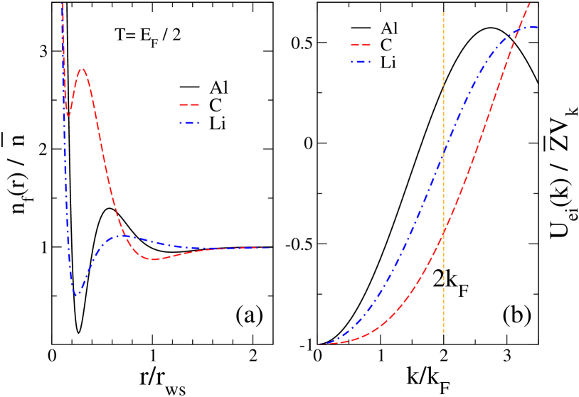
Figure 1: (Color online) Free-electron densities and pseudopotentials for the elements Al, C, and Li. (a) The NPA free-electron density $n_{f}(r)$ normalized by the average free-electron density $\bar{n}$ for Al³⁺, C⁴⁺, and Li⁺ at $\theta=T/E_{F}$=0.5, at densities $\bar{\rho}=$ 2.7 g/cm³, 3.7 g/cm³, and 0.513 g/cm³ respectively. Different elements are best compared using scaled lengths $x=r/r_{\rm ws}$ and scaled momenta $q=k/k_{F}$ where $k_{F}$ is the Fermi momentum. (b) The electron-ion pseudopotential $U_{ei}(k)$ via Eq. (2) is given in terms of the bare point-ion potential $\bar{Z}V_{k}$. That is, the form factor $M_{k}=U_{ei}(k)/\bar{Z}V_{k}$ is unity for an unscreened point-ion. The behaviour of the pseudopotential for values of $k/k_{F}$ significantly greater than 2 is unimportant.

In Eq. (2), the pseudopotential $U_{ei}(k)$ is re-expressed in terms of the point-ion potential $\bar{Z}V_{k}$ and the form factor $M_{k}$ which is unity only for an unscreened point ion. Here $U_{ei}(k)$ is a simple local $s$-wave potential and we have found it adequate for quantitatively reproducing results obtained from QMD where advanced non-local pseudopotentials have been used. The resulting pseudopotentials are shown in Fig. 1(b). The pseudopotentials can be fitted to a Heine-Abarankov form Utah12 , or more detailed parametrizations as provided in Ref. ELR98 .

For completeness we note that these pseudopotentials reduce to popular variants of the Yukawa potential  SunDai-Yuk17 ; Stanton15 ; Garavelli91 ; CDW-RT-81 ; Rogers70 ; Yukawa35 when the form-factor is set to unity and the $k\to 0$ limit of the Lindhard function is used as the response function. Then the screened pseudopotential becomes

$$U_{ei}(k)/\epsilon(k) = -\bar{Z}/(k^{2}+k_{s}^{2}),$$ (3)

$$\epsilon(k) = 1+k_{s}^{2}/k^{2},$$ (4)

where the $k\to 0$ limit of the random-phase approximation (RPA) to the dielectric function $\epsilon(k)$ has to be used. Such models become accurate in the high-density, $\theta\to 0$, Gell-Mann - Brueckner limit where the Yukawa potential becomes the Thomas-Fermi screened potential, and in the low density, high-temperature limit ($\theta\gg 1$) of Debye-Hückel-like systems. The intermediate case and related approximations are discussed in Ref. CDW-RT-81 . The form proposed by Stanton and Murillo Stanton15 is a partial linearization based on the Thomas-Fermi-Weizsäcker finite-$T$ density at an atomic nucleus, but still in the long-wavelength ($k\to 0$) limit. Finite-$T$ screening at finite-$k$ based on the homogeneous-electron-gas RPA model is the next step beyond the Yukawa form and has been studied by Perrot perrotRPA91 . We have improved on these in the NPA potentials in two ways: (i) we go beyond the RPA by using a local-field correction that satisfies the finite-$T$ compressibility sum rule in regard to the response function, and (ii) we go beyond the point-ion or Thomas-Fermi-Weizsäcker models by employing a form factor and incorporating the full non-linear Kohn-Sham density response in the electron-ion interaction $U_{ei}(k)$. This is done by the simple procedure given in Eq. (2).

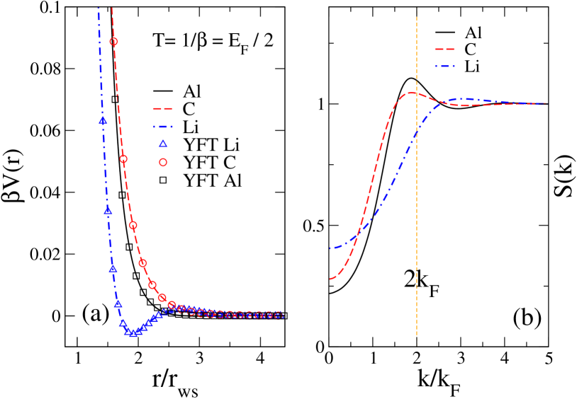
Figure 2: (Color online) Pair potentials $V(r)$ and structure factors $S(k)$ for Al, C, and Li at the same conditions given in the caption of Fig. 1. (a) The ion-ion pair potentials $V(r)/T$ for C, Al, and Li are computed from the pseudopotentials $U_{ei}(k)$ (see Fig. 1(b)) using Eq. (2). The $V(r)$ is accurately parametrized by the YFT form (see Sec. III). The YFT fits are shown as symbols (triangles, circles, or squares) and data from the NPA calculations are shown as solid lines. (b) Ion-ion structure factors $S(k)$ are obtained from the pair potentials $V(r)$ using the MHNC equation. At low temperatures when, $\theta<0.25$, the Friedel oscillations are significant; the Friedel oscillations become more damped when $\theta=0.5$.

II.2 The pair potential

Neutral pseudoatoms are non-interacting objects and their free energies are additive quantities. It is the unscreened pseudoatoms (ions of charge $\bar{Z}$ free of their screening sheaths) that interact. The pair potential is the interaction energy between an unscreened pseudo-ion in the presence of another unscreened pseudo-ion, at a distance $r$ apart in the medium containing only a uniform electron subsystem, while a static (non-responding) neutralizing positive-ion background is implicit. This interaction between two unscreened pseudo-ions is just their Coulomb interaction moderated by the screening effect of the electron subsystem. The pseudopotential was constructed by “unscreening” the pseudoatom density using linear response theory, as in Eq. (2). Hence the use of linear-response theory to determine the effect of screening on the pair interaction is appropriate, and corresponds to second-order perturbation theory using the pseudopotential $U_{ei}(k)$.

Using Eq. (2), the ion-ion pair potential in Hartree atomic units is

$$V_{ii}(k) = \bar{Z}^{2}V_{k}+|U_{ei}(k)|^{2}\chi(k),$$ (5)

$$= Z^{2}V_{k}+|\Delta n_{f}(k)|^{2}/\chi(k,T)$$ (6)

Equation (5) has been used in the theory of liquid metals since the 1960s but with empirical pseudopotentials. Here we use the NPA based first principles pseudopotentials to construct the interaction between two unscreened pseudo-ions of the same type Perrot90 . The form given in Eq. 6 emphasizes the non-linear DFT density pileup $\Delta n_{f}(k)$ and indicates that the linear-response assumption is contained in using $\chi(k,T)$ as the electron response.

The interaction between two unscreened pseudo-ions of different types immersed in the same electron subsystem, at the temperature $T$ is given by,

$$V_{ij}(k)=\bar{Z}_{i}\bar{Z}_{j}V_{k}+U_{ei}(k)U_{ej}(k)\chi(k).$$ (7)

Here the ions have charges $\bar{Z}_{i}$ and $\bar{Z}_{j}$ and pseudopotentials $U_{ei}(k)$ and $U_{ej}(k)$. As before, the pseudopotential used here is also the simplest local ($s$-wave) pseudopotential; no angular-momentum projected (non-local) forms have been found necessary in our studies of uniform WDM fluids or even for calculations on cubic solids using NPA HarbEOSPhn17 . In contrast, $N$-atom QMD calculations of such systems often employ non-local potentials. The simple pseudopotential in NPA arises from the fact that the NPA does not attempt to account in detail for directional bonding when spherical averages suffice.

The $r$-space form of the pseudopotential is obtained by Fourier transformation, and hence the calculation of pseudopotentials and pair potentials from the NPA within linear response is computationally rapid, and provides accurate DFT results for single-component systems. A discussion on using this NPA approach for multi-component systems is presented in Sec. VII.3 and follows Ref. eos95 . In describing the general method we use a discussion based on a single-component system with the ions and electrons all in equilibrium at a temperature $T$. Thus the ion-ion linear response pair potential $V_{ii}(r)$ will be denoted by $V(r)$ where no ambiguity arises. The pair potentials for systems where the electron temperature $T_{e}$ is different from the ion temperature $T_{i}$ may be generated as presented in Harbour et al. DSF18 .

The pair potentials for Al, C, and Li are displayed in Fig. 2(a); they are computed from Eq. (5) using the pseudopotentials shown in Fig. 1(b). The corresponding ion-ion structure factors $S(k)$ are computed from the modified hyper-netted-chain (MHNC) equation and are displayed in Fig. 2(b). We stress that the NPA model holds for arbitrary electron-ion systems ranging from low to high temperatures as long as the main assumption of the validity of linear response is upheld. Starting from the pseudopotential, pair potential, and structure factor generated from NPA, it is possible to determine the thermodynamic properties as well as linear transport properties eos95 ; cond3-17 of the system. For example, the EOS and thermodynamics can be obtained directly from the total free energy. Electrical transport coefficients like the electrical conductivity can be computed from Ziman-type formulae from Kubo-Greenwod theory, or from Fermi golden-rule type considerations Utah12 . Ionic transport properties like diffusion and viscosity can be obtained from the Green-Kubo relations by using the the pair potentials as an input to classical MD simulations Stanek21 .

A comparison of the pair potential obtained with the NPA model and QMD calculations for C is displayed in Fig. 3, showing excellent agreement. Many other comparisons were given in Ref. Stanek21 also showing reasonable agreement for many elements at various average densities and temperatures. The electrons have been eliminated from such potentials which require three-center (and higher) terms in the total free energy $F$. In contrast, the NPA retains contributions to $F$ from the two-component system of free electrons and ions, pair interactions, and their XC-contributions to the free energy that merely depend on the electron-sphere radius $r_{s}$ and $T$ (see Sec. VII).

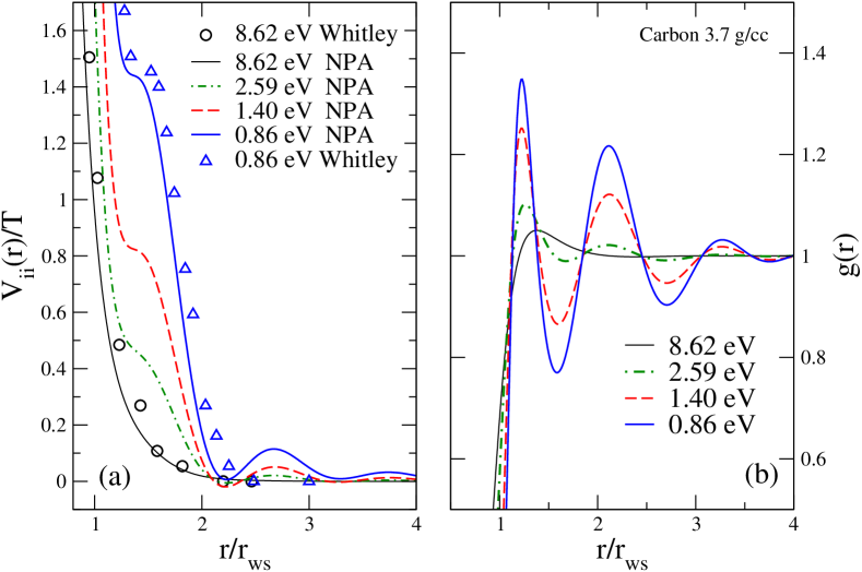
Figure 3: (Color online) (a) The QMD pair potentials of $l$-C at $\bar{\rho}$ = 3.7 g/cm³ by Whitley et al.. whitley15 are compared with the NPA linear-response pair potentials, Eq. (5), from $T=$ 0.86 eV to 8.62 eV. The QMD potentials fail to recover the Friedel oscillations (for $r/r_{\rm ws}>3$) seen in the NPA potentials and may not, for instance, capture long-range correlations important at phase transitions. (b) Two illustrative examples of the YFT fits to the pair-potentials (log-$y$ scale). The potentials are nearly Yukawa like at higher $T$, but develop Friedel oscillations at lower $T$.

It is important that the pair potential is accurate in the regime of radial distances $r>r_{\rm ws}$ since neighbouring atoms are usually located in shells that follow the stationary points (minima or inflection points) of the Friedel oscillations of the pair potential where possible. So, the Kohn-Sham equations of the NPA are solved for $R_{c}\sim 10r_{\rm ws}$ (or 5$r_{\rm ws}$ at higher $T$), unlike in many AA models where the free-electrons are confined to the Wigner-Seitz sphere. As the particle correlations become weak at higher temperatures, a smaller $R_{c}$ can be used in NPA calculations since Friedel oscillations become increasingly weak and die off within a short range.

III Yukawa Friedel-Tail potential: A general parametrized form of the pair potential

The ion-ion pair potential, given in Eq. (5), when Fourier transformed gives a numerical form for $V(r)$. Since various model forms based on the Yukawa potential and its modifications have been studied in the context of WDM, it is of interest to examine the structure of $V(r)$ and provide a general physical model that can successfully parametrize these potentials accurately, using only a minimum of parameters that also have a physically clear meaning.

Such a model consists of a Yukawa-screened ion carrying a long-ranged Friedel tail referred to in the following as the “YFT” model. Here, we provide parametrizations for Al, C, and Li as examples of YFT potentials. We find that the model is useful even in regimes where the NPA technique becomes inaccurate, for example, for low-density low-temperature $l$-C, as shown by Stanek et al. Stanek21 . The FM low-density low-temperature potentials obtained from QMD simulations using Eq. (1) do not recover many Friedel oscillations due to finite-size effects. However, the FM potentials can be reliably extended by fitting to the YFT model explicitly given in Eq. (8).

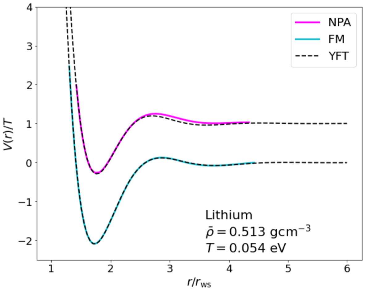
Figure 4: (Color online) A comparison of the results of fitting the YFT model, Eq. (8), to parametrically represent the NPA and FM pair potentials for Li. The FM pair potential from QMD is extracted from QMD simulations using Eq. (1) Stanek21 , while the NPA pair potential is obtained from Eq. (5). The YFT model correctly captures the structure of the pair potentials and allows an extension of the FM potential to a wider range in $r$. The NPA potential and the corresponding YFT fit have been shifted by unity for visual clarity.

The YFT form of the potential used is taken as a sum of a Yukawa form $V_{\rm y}(r)$ and a thermally damped Friedel tail $V_{\rm ft}(r)$

$$V_{\rm yft}(r) = V_{\rm y}(r)+V_{\rm ft}(r),$$ (8)

$$V_{\rm y} = (a_{\rm y}/r)\exp(-k_{\rm y}r),$$ (9)

$$V_{\rm ft} = (a_{\rm ft}/r^{3})\exp(-k_{\rm ft}r)\cos(q_{\rm ft}r+\phi_{\rm ft}).$$ (10)

Here the Yukawa form has a screening constant $k_{\rm y}$ which is of the order of the finite-$T$ Thomas-Fermi screening length, while a different $T$ and $\bar{n}$ dependent screening constant $k_{\rm ft}$ defines the thermally damped Friedel oscillations. The Friedel oscillations have the usual form: a circular function phase-shifted by $\phi_{\rm ft}$ and modulated by a $1/r^{3}$ decay. This six-parameter fit form is found to be capable of accurately reproducing the pair potentials of all the WDM systems containing free electrons and ions that we have studied ranging from very low temperatures close to the melting point, to temperatures typical of the plasma state. At higher temperatures and higher compressions, the interaction potentials become simpler and Yukawa-like, with the Friedel oscillations becoming increasingly damped Stanek21 . Hence the potentials discussed here focus on the more demanding regime of WDM systems, i.e., from close to the melting temperature to about $\theta\sim 1$. In the Yukawa-like high-$T$ high-density regimes, Thomas-Fermi models and their extensions like the orbital-free molecular dynamics method can increasingly supplant $N$-atom DFT calculations. However, even in the high-$T$ range, the NPA provides a wealth of information (via its Kohn-Sham states), ion-ion PDFs etc., that are not available from Thomas-Fermi models or their extensions to “orbital-free” techniques, while being computationally very efficient.

The six parameters $a_{\rm y},k_{\rm y},a_{\rm ft},k_{\rm ft},q_{\rm ft},$ and $\phi_{\rm ft}$ can only be approximately estimated using analytical models of screening. This is partly because they are also playing the role of fitting to the form factors contained in the actual NPA potentials that account for the finite size of the ionic cores. Hence they are best obtained by fitting the NPA-derived numerical pair potentials to the YFT fit form Eq.(8). The simple least-square fitting routines available in standard open-source software or graphics packages (e.g., gnuplot or python) are sufficient for obtaining the fit parameters of Eq. (8). The fitted forms can then be used as inputs to classical MD simulations. For example, these fitted potentials can be used in systems with density gradients that can be described by a graded stack of layers of uniform density and width not less than the radius of the correlation sphere, viz., $R_{c}\sim 5r_{\rm ws}$.

Furthermore, the fitted pair potentials can be compared with the pair potentials derived from force matching to QMD simulations if FM potentials are available. Since $N$-atom QMD calculations are carried out in a simulation box of linear dimension $\sim r_{\rm ws}N^{1/3}$, the $N$-center potential energy surface used in force matching is itself of restricted range, and long-ranged oscillations are only poorly recovered in force-matched potentials unless a large number of particles are used. We illustrate this by comparing the QMD-derived C pair potential shown in Fig. 3(a) due to Whitley et al. whitley15 and the Li pair potential shown in Fig. 4 due to Stanek et al. Stanek21 . Such QMD-derived pair potentials can be approximately extended to include their long-ranged Friedel oscillations in two ways: ( i) they can be augmented with the Friedel tail obtained from YFT fits to NPA pair potentials or (ii) the YFT form can be fit directly to the QMD data. The parametrized forms can be analytically differentiated or manipulated more efficiently and more accurately than numerical tabulations or ML potentials.

III.1 General applicability of the YFT model

In the present study we explicitly provide comparisons of NPA pair potentials and those obtained from QMD force matching. The tabulations of parametrizations given below involve a temperature span of a factor of 10 from the lowest temperature treated. At higher temperatures, the pair-potentials become Yukawa-like which simplifies the YFT model accordingly by damping out the Friedel tails. As shown by Stanek et al. Stanek21 , the agreement between the NPA and FM pair potentials is usually quite good. Furthermore, we note that the pair potentials generated via the NPA method are consistent with the YFT model as the NPA model used here contains an automatic check for a YFT-type construction that has been used for the simplifications of subsequent numerical applications of the potentials. Hence, all the curves marked NPA in the figures have YFT fits that adequately reproduce the numerically tabulated NPA or FM pair potentials.

It is interesting to note that many of the available AA models become accurate mainly at the higher-$T$, higher-density regimes which are the regimes where the pair potentials become Yukawa-like as the Friedel tails become negligible. Similarly, the PIMC method also works best at higher temperatures where the effects of the Friedel tails are negligible. We illustrate this in detail using the YFT fits to WDM Al (see Sec. V) from $T=8$ eV to 100 eV. Results for WDM Li and C are also given up to 100 eV and comparisons with other methods are given when available.

IV Parametrized Carbon Potentials

Table 1: The parameters of the YFT potential $V(r)/T$ for C. The fits are for approximately the range $0.8<r/r_{\rm ws}<4$ and cover up to $\sim 3$ to 4 units in the energy scale of $V(r)/T$ as shown in Fig. 7. Force-matched pair potentials Stanek21 using Eq. (1) have been used at the density $\bar{\rho}$ = 2.267g/cm³ and fit to the YFT form while the NPA pair potentials, Eq. (5), have been used for the higher-density YFT fits.

$\bar{\rho}$ [g/cm${}^{3}]$	2.267	2.267	3.5	3.5	5.0	5.0	10.0	10.0
$T$[eV]	1	2	1	2	1	2	1	2
$a_{\rm y}$	70.2535	43.4002	167.769	105.664	280.957	164.833	492.126	273.037
$k_{\rm y}$	1.23545	0.897833	1.34858	1.42488	1.46306	1.53154	1.70158	1.75576
$a_{\rm ft}$	60.2645	15.5518	54.2138	27.5023	23.2234	12.7514	6.04252	3.33661
$k_{\rm ft}$	0.421458	0.878615	0.378277	0.403479	0.255881	0.295816	0.000006	0.0334616
$q_{\rm ft}$	2.23931	2.39948	2.86869	2.84593	3.20147	3.17996	3.97784	3.93940
$\phi_{\rm ft}$	3.36746	2.75123	2.49232	2.57176	2.12173	2.22056	1.50360	1.60452

Liquid C is usually considered to be a highly covalently bonded system even in the fluid state. This view is supported by “snap-shots” of real-space positions of the ions obtained from QMD simulations. The multi-center bond-order potentials Abell85 ; Brenner02 ; ghiring05 use this chemical picture to model MCPs for C systems. However, as is evident from DFT, only the long-time average is relevant to determining the thermodynamics and static structure factor since the effects of the transient bonds average out in $l$-C DWP-carb90 . In QMD, this average is explicitly carried out using millions of configurations of solid-like ionic clusters, without taking advantage of the spherical symmetry of the fluid or the possibility of using an ion-ion XC-functional to treat many-center effects. While the chemical-bonding picture does not use the Fermi-liquid character of $l$-C, the NPA approach exploits it to the fullest extent in the YFT model.

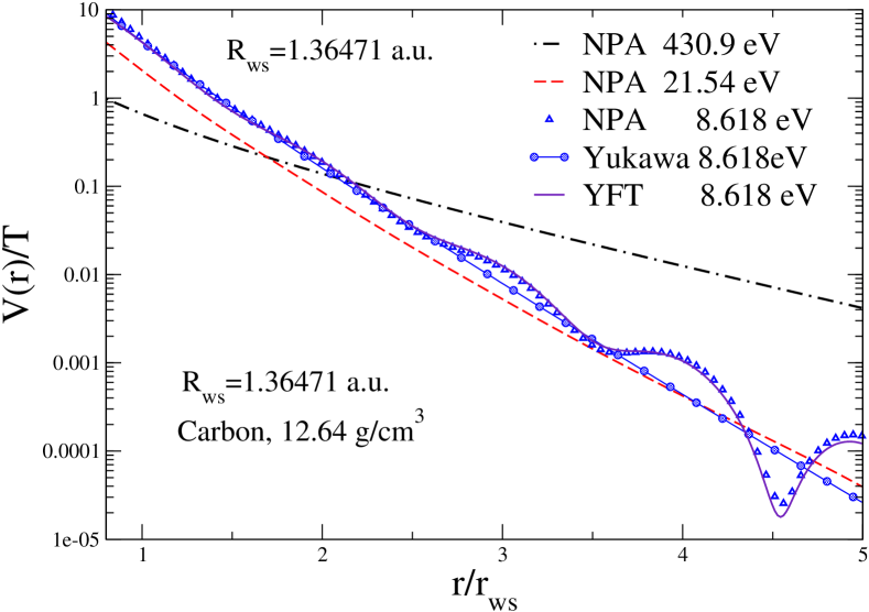
Figure 5: (Color online) The NPA C-C pair potentials for WDM C studied by Driver et al.. driver12 . The $y$-axis ($V(r)/T$) is logarithmic and the quasi-linearity of the plots for $V(r)$ at $T=430.9$ eV and 21.54 eV establish the Yukawa-like character of the pair-potentials. At $T=8.618$ eV, the pair potential contains Friedel oscillations for $r>1.5r_{ws}$; the NPA potential is well fitted by the YFT form.

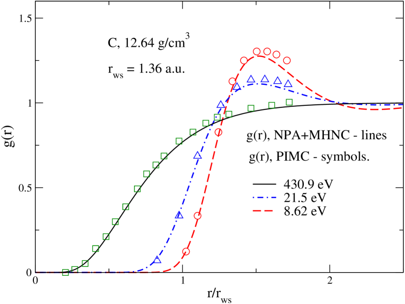
Figure 6: (Color online) The C-C PDFs $g(r)$ from the NPA potentials, from PIMC and QMD of Driver et al. driver12 .

We calculate the NPA pair potentials and the $g(r)$ of $l$-C, at density 12.64 g/cm³, at $T=8.62$ eV (1x$10^{5}$K), 21.5 eV (2.5x10⁵K), and 430.886 eV (5x10⁶K) to compare with the PIMC and QMD calculations of Driver and Militzer driver12 . The mean ionization $\bar{Z}$ obtained from the NPA changes from $\bar{Z}=4.0$ at low $T$, to $\bar{Z}=4.05$ by $T=100$ eV, and reaches $\bar{Z}=5.758$ by $T=430.9$ eV – the highest $T$ used by Driver and Militzer driver12 .

The YFT fits to the NPA potentials that reproduce the PIMC $g(r)$ data even at low-$T$ and at lower density are given in Fig. 5. The comparison of the NPA $g(r)$ obtained from the NPA potentials with the $g(r)$ from PIMC are given in Fig. 6. The NPA $g(r)$ are obtained from the pair potentials using the MHNC equation. This is an inexpensive alternative to carrying out an MD simulation. We caution that if using MHNC in place of MD, one needs to specify an accurate bridge function in the MHNC equations. Additionally, although hard-sphere approximations to the bridge function are often employed in the MHNC equations by appealing to a universality principle Rosenfeld93 , it should be used with some care as this model may not be valid for certain systems. For example, the bridge function can be set to zero for C, Si, and Ge in the liquid state at normal densities, and near their melting points when their structures are controlled mainly by the scattering of electrons by ions from one edge of the Fermi surface to the opposite edge, giving rise to $2k_{F}$ scattering effects cdw-carb22 that control the ionic structure, rather than packing effects.

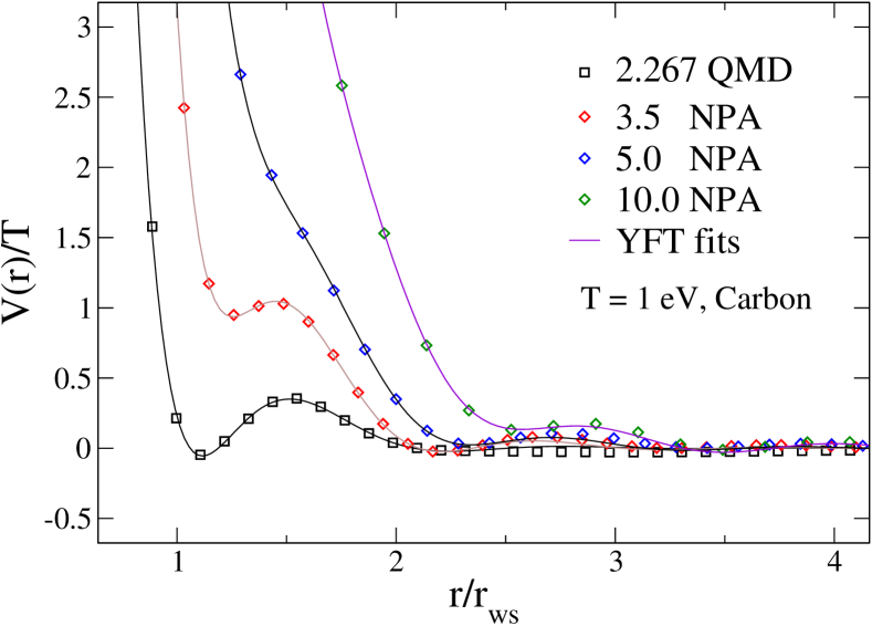
Figure 7: (Color online) The C-C pair potentials generated from FM and NPA (denoted by shapes) and their parametrized forms (continuous lines) based on the YFT model. The curves are identified by the numerical value of the corresponding systems density. The curve 2.267 QMD is the C-C pair potential obtained by FM to QMD data using Eq. (1) for $\bar{\rho}$ = 2.267 g/cm³ at $T=1$ eV Stanek21 . The pair potentials at higher densities were generated using the NPA, Eq. (5), as indicated in the legends.

In Table 1, we present a sample of parametrizations for the YFT potentials for C along the $T=1$ and 2 eV isotherms, for the range of densities $\bar{\rho}=2.267$ g/cm³ up to 10 g/cm³. At higher $\theta$ and higher densities, the potentials increasingly approximate a Yukawa-like form. The linear response potentials are applicable for $\bar{\rho}\geq$ 3 g/cm³ where they recover the structure factor and pressure obtained via QMD simulations cdw-carb22 . The low-density range from $\bar{\rho}<3$ g/cm³ and extending towards the graphite density and below, cannot be accurately computed using the linear-response model given by Eq. (2). Therefore, we use a FM pair potential to construct a parameterization with the YFT model and provide parameters for the density $\bar{\rho}=2.267$ g/cm³. We note that the mean ionization of C is such that $\bar{Z}=4$ for the densities and temperatures studied here.

Higher densities and temperatures (e.g., 10-100 times the diamond density and in the 10⁶ K temperature range) have been studied using the NPA cdw-Carbon10E6-21 , and the pair potentials under such conditions can be accurately fitted to the YFT form. To illustrate the fact that the YFT potentials reduce to simple Yukawa-like potentials for sufficiently high-$T$, we give the parametrizations for the Yukawa-like pair potentials of $l$-C at the graphite density in Table 2 of Appendix B.

The parameters given in Table 1 reflect the character of a screened metallic ion. This is confirmed by the value of the screening constant $k_{\rm y}$ which is quite close to the Thomas-Fermi screening wavevector, while the wavevector $q_{\rm ft}$ associated with the Friedel oscillations, is approximately 2$k_{F}$; the Friedel oscillations decay as $1/r^{3}$ as expected for a metallic fluid. The screening constant $k_{\rm ft}$ introduces a damping of the Friedel oscillations. For systems such that $\theta$ is small, this damping constant may be set to zero and the Friedel oscillations are similar to those familiar in metal physics. Since the $l$-C systems studied here are such that $\theta$ is very small, we could have set $k_{\rm ft}=0$ and used a simpler five-parameter fit which is equally capable of fitting to the QMD or NPA data. We will make this simplification for treating $l$-Al as is done in Sec. V and presented in Table 3.

V Parametrized Aluminum Potentials

We study normal density Al from $T=0.5$ eV to 100 eV, and in the density range $\bar{\rho}=$ 2.0 g/cm³ to 6 g/cm³ at $T=1$ eV. The normal solid-state density $\bar{\rho}$ is 2.7 g/cm³, while the isobaric $\bar{\rho}$ is 2.375 g/cm³ at its melting point ($T=$ 933.47 K). Unlike the C ion with $\bar{Z}=4$ which is almost point-like – having only the 1$s$ of bound electrons – Al³⁺ has a large core and its form factor is an important feature of its pseudopotential. Nevertheless, we find that the YFT model works satisfactorily for $l$-Al as well because the YFT parameter set is flexible enough for doing “double duty”. What we mean by this is that the parameters of the YFT model have more fitting capacity than would be found in a strictly defined physical model. Such a strictly defined model would require a parametrization of the form factor of the pseudopotential and a parametrization of the electron response function, so that Eq. 5 is itself fully parametrized.

A highly non-local pseudopotential rather than the simple $s$-wave form has been used in linear-response DRT75 and in QMD codes like the VASP VASP and ABINIT ABINIT although we find this to be unnecessary in NPA applications to uniform-density systems and cubic solids. Liquid Al differs from $l$-C in that the main peak of the structure factor is not located at 2$k_{F}$ as in C, Si, and Ge cdw-carb22 at their typical densities. The YFT parameters that fit the NPA potentials for $l-$Al are given in Table 3 of Appendix B. The WDM form of $l$-Al very close to its melting point, and under more extreme conditions have been studied using the NPA and reported in previous publications eos95 ; cond3-17 ; PDWBenage02 .

The Friedel oscillations in $V(r)$ are of great importance for the potential near the melting point of Al. Under these conditions, the first peak of the $g(r)$ locates at a positive energy turning point of a Friedel oscillation DRT75 ; cdw-aers83 ; HarbEOSPhn17 ; DSF18 . The NPA potentials between $T=$0.5 eV and 9.0 eV have been compared with FM potentials obtained using Eq. (1) from QMD simulations Stanek21 . In Fig. 2 we show two cases of Al at $\bar{\rho}=2.7$ gcm^-3, viz., one for $T=$ 0.5 eV and another for $T=$ 9.0 eV. The $T=$ 0.5 eV case is typical of the YFT regime where Friedel oscillations are non-negligible, whereas the $T=$ 9.0 eV case typifies the regime where the Friedel oscillations have become sufficiently damped and the YFT potential is approximately Yukawa-like.

At low-$T$, the NPA potentials have oscillatory tails while the FM potentials capture them only partly, as already seen in the C potentials in Fig. 3(a). However, the FM pair potentials and the more oscillatory NPA potentials nevertheless yield PDFs and ion-ion structure factors that are in close agreement. By $T=9.0$ eV, which corresponds to $\theta=0.77$, the potentials are no longer oscillatory and only the Yukawa form remains. This is in fact often the case by $\theta\gtrsim 2/3$ even at other densities, and for many elements. As $T$ increases, $\theta$ increases and the Yukawa approximation improves, but this is modified by changes in the mean ionization $\bar{Z}$ which increases $E_{F}$, thereby countering the accuracy of the Yukawa form. Nevertheless $\theta$ steadily increases in WDM Al from $\theta=1.549$ for T = $20$ eV where $\bar{Z}$ = 3.495 to $\theta=4.567$, for T = 100 eV where $\bar{Z}$=7.721. Thus the Yukawa form continues to be a reasonable approximation in spite of increased ionization; the values of the parameters for the range $T=8$ eV to 100 eV for normal density Al is given in Table 4 of Appendix B.

Although the potentials have become Yukawa-like, the ion-ion $g(r)$ and $S(k)$ are still strongly coupled as the plasma parameter $\Gamma=\bar{Z}^{2}/(r_{\rm ws}T)$ exceeds unity, being $\Gamma=8.35$ at $T=10$ eV and $\Gamma=6$ at $T=80$ eV. Hence $g(r)$ must be computed using MHNC or with MD. A simple but useful approximation may be obtained by a one-component-plasma analogy based on the value of $\Gamma$ Clerouin14Gamma . The fact that the potentials reduce to Yukawa-like forms in at least the $\theta\gtrsim 1$ regime opens the door for a semi-analytic theory of these WDM systems for a wide range of conditions.

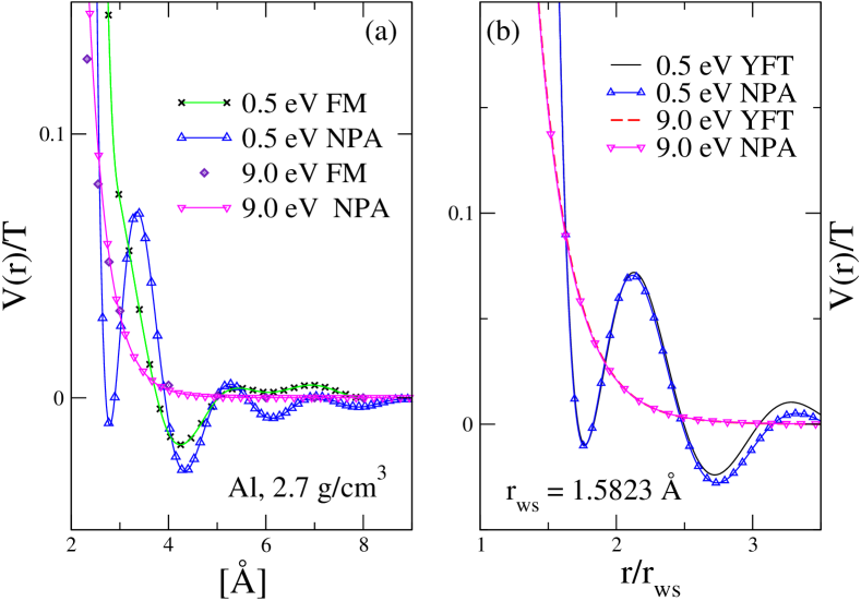
Figure 8: (Color online) (a) The Al-Al pair potential at $\bar{\rho}$ = 2.7 g/cm³ from NPA, Eq. (5), and from FM using Eq. (1) on QMD data Stanek21 , for temperatures $T=$ 0.5 eV and 9 eV. The oscillatory terms seen in the NPA potential, larger at the melting point ($T=$ 0.083 eV), are already less than a tenth of the thermal energy by $T=$ 0.5 eV, and the FM pair potentials recover an average value. (b) The NPA potentials and the YFT fits in the region relevant to the main peak-structure of $g(r)$. The YFT fit reduces to a Yukawa form at $T=$ 9 eV .

In fitting the NPA potentials to the YFT form we have simply used no thermal damping on the Friedel term ,i.e., setting $k_{\rm ft}$ equal to zero. This shows that the parameters of the fit form “do double duty” and their values are not necessarily related to the values expected from basic theoretical models, although quite close to them. This fortunate flexibility is partly associated with the freedom in the selection of the range of $r$ used in the fits. Standard pseudopotential formulations also have such flexibility arising from how the atomic core is excluded in the pseudopotential. In general, the fit range is selected to be that of the ion-ion $g(r)$, viz $r_{\rm ws}\leq r<R_{c}$.

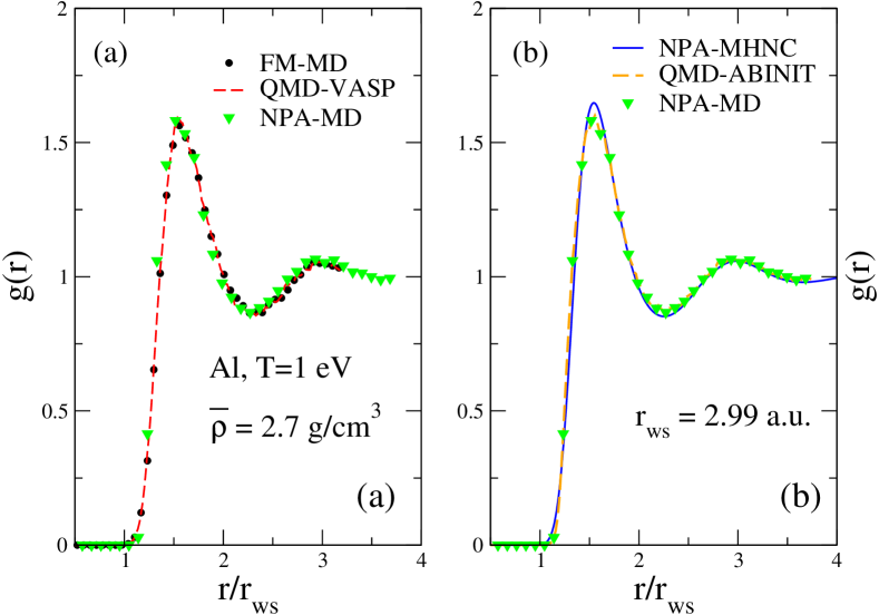
Figure 9: (Color online) (a) The PDF $g(r)$ of Al at $T=$ 1 eV and $\bar{\rho}=$ 2.7g/cm³. The PDFs are generated using QMD Stanek21 and MD with the FM and NPA pair potentials. (b) The PDF from QMD DSF18 and with the NPA pair potential, Eq. (5). The NPA PDFs are generated from MD and also with MHNC. The NPA-MD and the FM-MD agree closely although the NPA potential has more oscillatory structure as seen in Fig. 2.

It should be noted that the pair potential defined by Eq. (5) does not contain interactions with the polarizable atomic cores of the two interacting Al ions, or van der Waals interactions. The YFT fit-forms also do not specifically contain such interacting terms, although the parameters have some flexibility to absorb such contributions approximately. How these concerns could be included within a purely DFT scheme were discussed in the Appendix of Ref. eos95 . These concerns are also important in systems that contain a significant mixture of neutrals, e.g., Ar plasmas at $T\sim$ 1$-$2 eV and normal density Stanek21 where an argon mixture is treated using g the NPA. At the temperatures and densities considered here, the dominant interactions are those included in Eq. (5), and hence we will not discuss core-polarization effects further.

In Fig. 9(a) we compare the $g(r)$ generated directly within QMD, and labeled QMD-VASP with the $g(r)$ obtained from MD using the FM potential extracted from the QMD using Eq. (1). In Fig. 9(b) we compare the $g(r)$ generated directly from QMD using ABINIT, with the PDFs obtained from the NPA pair-potential using MD, and using MHNC DSF18 , showing that the MHNC yields $g(r)$s of good accuracy. We may also note that the NPA pair potential provides an $S(k)$ for Al that not only agrees with the static $S(k)$ obtained by QMD simulations, but also accurately renders the dynamic ion-ion structure factor $S(k,\omega)$ obtained from DFT-MD microscopic simulations available at $T=$ 1 eV and at $\bar{\rho}$ = 2.7 g/cm³ DSF18 .

VI Parametrized Lithium Potentials

Lithium in its WDM state has not been as extensively studied as Al or C. However, accurate data for the structure factor $S(k)$ of $l$-Li near its melting point as well as attempts at theoretical predication are available Salmon2004 . Since theories should preferably be tested against actual experimental data rather than against simulation results, we first study this case, i.e., $l$-Li at $\bar{\rho}$ = 0.513(4) g/cm³ and at a temperature of $T=$ 197^∘C (which corresponds to $T=0.0405$ eV in the units used here). At this very low temperature and nearly the solid-state density, it is easy to imagine that pair potentials would be totally inadequate and that a multi-center approach would be needed. However, our results show that the NPA pair potential, taken together with the MHNC integral equation where the bridge term is modeled by a hard-sphere fluid very successfully predicts the experimental data. The packing fraction $\eta=0.3$ of the hard-sphere fluid is determined using the Lado-Foiles-Ashcroft free-energy minimization criterion LFA83 .

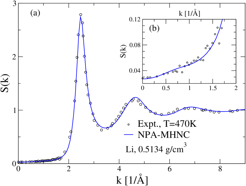
Figure 10: (Color online) (a) The neutron-scattering structure factor of Li at $T=$ 470 K is displayed as circles, $S(k)$ Salmon2004 . It is compared with the theoretical $S(k)$ from the NPA-MHNC calculation. The bridge contribution is that of a hard-sphere fluid with a packing fraction of $\eta=0.3$, given by the Lado-Foils-Ashcroft criterion. The inset (b) shows the low-$k$ behavior and the accurate recovery of the $k\to 0$ limit required to satisfy the compressibility sum rule. The Li-Li NPA pair potential for this case, $\bar{\rho}=0.5134$ g/cm³ is displayed in Fig. 11.

Stanek et al. Stanek21 have compared the NPA potential and its predictions for Li at $\bar{\rho}=0.513$ g/cm³ and $T=0.054$ eV, with those from FM potentials obtained from QMD simulations using Eq. (1), obtaining excellent agreement. As the Fermi energy of Li at this density is $E_{F}\sim$ 5 eV, with $\theta\simeq 0.011$, the electron subsystem is effectively highly degenerate. The NPA potentials were found to work very well even for solid-density Li as the phonons calculated using the NPA pair potentials were in good agreement with experimental phonon dispersion data HarbEOSPhn17 . It has also been verified that the NPA pair potential for Li at $T=0.173$ eV generates PDFs in good agreement with the QMD data at $\bar{\rho}=0.85$ g/cm³ Kietzman08 .

While the above cases are for high-electron degeneracy, Harbour et al. cond3-17 found good agreement between QMD calculations of various aspects of X-ray Thomson scattering and those from NPA methods for the density $\bar{\rho}=0.6$ g/cm³ and $T=4.5$ eV. In this case, the electron system is at a temperature close to the Fermi energy and is partially classical in its behaviour. Hence we may conclude that currently available QMD data confirm the validity of the NPA potentials for WDM-Li from the solid state to the plasma state. A comparison of the FM Li-Li pair potential using Eq. (1) at $T=0.54$ eV and $\bar{\rho}=0.513$ g/cm³ and the corresponding NPA Li-Li potential is given in Fig. 11.

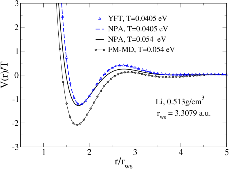
Figure 11: (Color online) The Li-Li pair potential. The FM pair potential obtained by Stanek et al. Stanek21 (denoted as QMD-FM) corresponds to Li at $\bar{\rho}=0.513$ g/cm³ and $T$ = 0.054 eV; the corresponding NPA pair potential calculated from Eq. (5) is given by solid lines. The NPA pair potential at $T=0.0405$ eV = 470 K is denoted by a dashed line and corresponds to a case for which neutron-scattering $S(k)$ data are available (see Fig. 10).

Unlike in the case of Al, the difference between the FM $V(r)$ and the NPA $V(r)$ at their minima is more significant compared to the case of Al at $T=$ 1 eV (Fig. 2), being of the order of the thermal energy of the system at $T=0.054$ eV. However, this difference is not reflected in the predicted properties, e.g., the $S(k)$ or $g(r)$ Li, as seen in Fig. 12 and Fig. 13 respectively. In Fig. 12 we show the $S(k)$ obtained from the HNC, i.e., MHNC with the bridge function set to zero as well as the MHNC with the proper LFA-optimized bridge term LFA83 , displaying the role of the bridge contribution to the ionic structure.

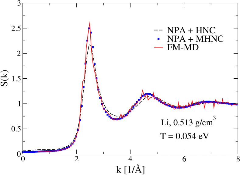
Figure 12: (Color online) The $S(k)$ from the NPA pair potential generated using HNC and MHNC, and from the FM pair potential, Eq. (1), using MD are displayed.

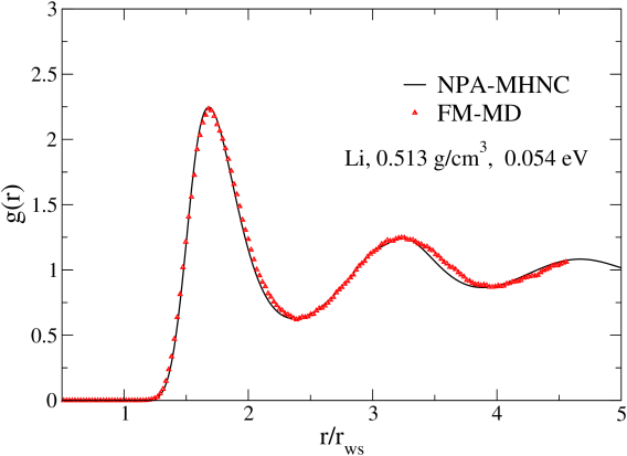
Figure 13: (Color online) The PDF $g(r)$ from the Li NPA pair potential generated using MHNC, and from the FM QMD pair potential Stanek21 , Eq. (1), using MD are displayed.

In Table 5 of Appendix B we provide YFT fits to Li-Li pair potentials generated using the NPA electron density and the linear-response pair potential given by Eq. (5). In most cases, we have set the parameter $k_{\rm ft}$ controlling exponential damping term of the Friedel oscillations to zero, except in the case of the density $\bar{\rho}=$ 0.85 g/cm³ where we have included it as a parameter, merely to illustrate the fact that there is significant interplay among parameters, and consequently, a numerical fit of similar quality can usually be obtained even if $k_{\rm ft}$ is set to zero. We give YFT fits for several densities from $\bar{\rho}=0.513$ g/cm³ to 1 g/cm³, and at temperatures $T=0.054$ eV and 1.0 eV in all cases. We also give the YFT fit at $T=4.5$ eV and $\bar{\rho}=$ 0.513 g/cm³ which corresponds to $\theta=0.983$ where the fit form reduces to a Yukawa form as the Friedel oscillatory term is found to be negligible. Just as in Al, we have a regime $\theta\gtrsim 1$ where the pair-potentials of the Li WDM system become Yukawa-like in spite of increasing ionization with increasing temperature. The Yukawa-like parameters that fit the NPA potentials in this regime are given in Table 6 of the Appendix B.

VII discussion

There are multiple motivations for constructing parametrizations of pair potentials based on an approximate physical model with very few parameters rather than using a highly flexible purely numerical approach fitted to QMD data. First, the parametrization provides some validation to the associated physical picture. Second, the fits can be used in simulation codes which call for repeated evaluations of the potentials and total energies as a function of position, temperature, and density. Third, the model potentials can be used to extend the domain of force-matched potentials $V(r)$ available only for values of $r$ restricted by the size of the simulation cell. Fourth, the existence of large regions of $\bar{\rho},T$ phase space where the Yukawa form of the pair potential raises the possibility of a semi-analytic theory of a wide range of WDM systems that are treated by AA, orbital-free-Thomas-Fermi type calculations.

The existence of a simple YFT-type parametrization of pair potentials in these WDM systems supports the physical picture of them being essentially metallic liquids; this being true even in the case of $l$-C or $l$-Si where a different paradigm has often been advanced, within the intuitive chemical picture of covalent bonding. The paradigm of “bond-order potentials” and their limitations in WDM applications are now well known. Just as the “bond-order potentials” may be used in simulation codes that call for repeated evaluations of the potentials, these YFT potentials may also be similarly used, much more simply. The method based on constructing FM potentials extracted from more fundamental DFT-MD simulations may become computationally prohibitive especially at higher temperatures, although the underlying physics for $\theta\gtrsim 1$ is Yukawa-like.

Standard DFT fails when ground states contain significant non-Born-Oppenheimer corrections, while excited states may involve conical intersections. Nevertheless DFT-MD is an excellent method for testing methods like the NPA, or in providing inputs to reference data bases for systems where the Born-Oppenheimer approximation holds and when experimental data are not available.

VII.1 Pair potentials, pair energies, and the total free energy

It should be noted that the pair potential $V(r)$ and the PDF $g(r)$ are sufficient to evaluate the pair-interaction energy $E_{12}^{int}$ (which is an excess energy referred to the non-interacting case) or the excess free energy among the ions inclusive of their correlation corrections. But an additional coupling constant integration using a potential $\lambda V(r)$ and a PDF $g(r,\lambda)$ with $\lambda$ varying from zero to unity is needed to obtain the ion-ion contributions $F_{12}$ to the free-energy. For instance, the “excess free-energy” which results from the ion-ion pair interaction beyond the mean-field energy is the ion-ion correlation energy. This can be written as a coupling-constant integration which may be conceptualized as replacing the ionic charge $\bar{Z}|e|$ by $\bar{Z}|e|\lambda$ where $\lambda$ is the charging parameter Onsager33 ; Kirkwood35 brought up to unity from the noninteracting value when $\lambda=0$. The coupling constant integration is Morita1960Theory ; Yan2004Statistical ; PDWXC

$$F_{12}/\bar{\rho} = \int^{1}_{0}d\lambda\bar{\rho}\int 4\pi r^{2}dr\frac{V(\lambda,r)}{\lambda}h(\lambda,r),$$ (11)

$$V(\lambda,r)/\lambda = V(r),$$ (12)

$$h(\lambda,r) = g(\lambda,r)-1.$$ (13)

An actual calculation by this method requires the evaluation of a sequence of ion-ion PDFs $g(\lambda,r)$ with a sequence of potentials $V(\lambda,r)$ for about a dozen values of $\lambda$ to carry out the $d\lambda$ integration. Such calculations have been done for simple potentials like the electron-electron Coulomb interaction in the context of calculations for the electron exchange-correlation energy at finite-$T$ PDWXC . However, if the HNC integral equation is used, then the above coupling constant integration can be avoided Silbert92 . Such a method has been implemented for warm dense plasmas in Ref. eos95 in the context of the NPA.

Equation (11) shows how the excess free energy of a pair of ions placed placed in the medium containing electrons and ions is related to the pair potential. The contributions beyond the mean-field energy contained in the many-body ion-ion interactions is brought in via their effect on the PDF $g(\lambda,r)$ via the charging process. At each charging step, as the interaction grows stronger, the weighting of correlations from, say, three-body terms brought in via the Ornstein-Zernike equation changes and contributes to the final value of the pair-energy. In the NPA model, the basic pair potential $V(\lambda,r)$ defines the direct correlation function $c(r)$ that enters the Ornstein-Zernike equation. In fact, asymptotically

$$c(\lambda,r)=-V(\lambda,r)/T.$$ (14)

The NPA’s structure, and how to extend it to include core-polarization effects and corrections to the kinetic energy functional that contribute to the pair potential etc., are described in Sec. 2 of Appendix B of Ref. eos95 . It does not include chemical bonding. In fact, persistent molecular ions arising from chemical bonding are compact entities that should be regarded as additional species present in the mixture.

The $F_{12}$ determines the ion-ion contributions to the internal energy, pressure, specific heats and other thermodynamic quantities. The coupling-constant integration can be explicitly carried out, say, for a dozen values of $\lambda$. Usually, even with such coupling constant integration, the NPA calculation of the free energy is computationally not heavy. However, we have found this coupling-constant integration, i.e., the $\lambda$-integration unnecessary as it can be side-stepped within the HNC integral-equation approaches, as discussed in Ref. eos95 , or by using reference hard-sphere-fluid models Pe-Be ; perrotRPA91 .

In effect, we may write the total Helmholtz free energy $F$ in terms of the contributions arising from the electrons, ions, and their interactions in the form Pe-Be ; eos95 :

$$F=F^{0}_{e}+F^{xc}_{e}+F_{em}+F_{12}+F^{0}_{I}.$$ (15)

The first two terms deal with the free energy of the non-interacting uniform electron fluid and its finite-$T$ exchange-correlation energy at the given density and temperature $T$. The last term, $F^{0}_{I}$ is the ideal (classical) free energy of the ion subsystem. The zero of energy may be assumed to be the infinitely separated set of nuclei and electrons, when the energy $E_{A}$ of $\bar{\rho}$ isolated atoms per unit volume (obtained from a standard atomic physics calculation) must be added to Eq. (15). This term eliminates itself in calculations of quantities like the pressure and specific heat as only differences in the free energy (derivatives) arise.

The third term, $F_{em}$ of Eq (15) is the embedding energy of the neutral pseudo-atom NPA in the uniform electron fluid. The fourth term, $F_{12}$ contains the interactions between unscreened pseudoatoms brought in via the pair potential, PDF, and the ion-ion correlation effects as already discussed in the context of the coupling-constant integration.

Given the average number of free electrons per ion (viz., $\bar{Z}$), the first three terms $F^{0}_{e},F^{xc}_{e}$, and $F^{0}_{I}$ at the given temperature are trivially evaluated. If an NPA calculation or an equivalent AA calculation is available, $F_{em}$ and $F_{12}$ are also available. Otherwise, approximate “universal” embedding energy functionals at finite-$T$ are available for use Zaremba85 . Hence, if parametrized pair potentials are available, classical MD methods may be used to calculate $F_{12}$, completing the evaluation of the full Helmholtz energy $F$, with respect to the reference zero of energy which may be conveniently taken to be the limit of infinitely separated neutral atoms, or alternatively, infinitely separated nuclei and electrons. Such calculations of the total free energy, internal energy and pressure, and electrical conductivity for Al, Be, C, H, Li, Si, etc., have been carried out in previous publications using the NPA method.

VII.2 Non-uniform systems

Consider a plasma with a density or temperature gradient along the $x$-direction; if the gradient region can be replaced by a sequence of uniform slabs, with a thickness not less than the correlation-sphere radius $R_{c}(x)$ in the direction of the density gradient, and a “thermal-energy thickness” of not more than $\bar{Z}(x)/r_{\rm ws}(x)$ in the direction of the temperature gradient, then the density and temperature dependent pair potentials of each slab can be used in the term $F_{12}$ of Eq. (15). The other terms in Eq. (15) are less complex and can be easily evaluated or interpolated using the density profile. Of course, this assumes that the varying density and temperature region does not traverse a phase transition or cause significant changes in the nature of the ions and hence the pair potential does not change strongly. Harbour et al.. HarbEOSPhn17 found surprisingly good results even when the method was applied to the near-surface region of an Al slab.

In the purely classical MCP approach, the expectation is that such gradients in temperature, density and ionization state are already covered by the ML algorithms that generated the potentials; hence a partitioning of the gradient region and quantum calculations for each of them are avoided. In many cases, when dealing with density or temperature gradients, doing a full NPA calculation for each density slab is quite easily done.

VII.3 Mixtures of ions

We briefly bring out the implications of the availability of parametrized potentials in dealing with mixtures. A more complete discussion of the NPA approach to mixtures is found in Ref. eos95 .

If we consider a simple mixture of $n_{s}$ species of ions, we need to specify $(n_{s}+1)n_{s}/2$ different pair potentials that can all be specified using only $n_{s}$ pseudopotentials (see Eq. (2)) and the average electron density (or, equivalently, $\bar{Z}$ of the mixture) which specifies the electron response function. However, a number of concerns have to be resolved before the theory can be exploited.

For example, if the WDM mixture is between two different ions having the same $\bar{Z}$, e.g., WDM Si and WDM C for which $\bar{Z}$ = 4 holds for a wide range of densities and temperatures, then the calculation of pair potentials and thermodynamics of such mixtures becomes trivial as the ionization balance is preserved.

However, if we consider a a sample of normal density ($\bar{\rho}$ = 2.7 g/cm³) WDM Al at any temperature up to about $T$ = 12 eV ($\sim E_{F}$), $\bar{Z}_{\rm Al}\approx 3$. We may isochorically replace a fraction of the atoms with Li atoms, to give composition fractions $x_{\rm Al},x_{\rm Li}=1-x_{\rm Al}$, with a mixture density $\bar{\rho}_{m}=x_{\rm Al}\bar{\rho}_{\rm Al}+x_{\rm Li}\bar{\rho}_{\rm Li}$, Unfortunately, it does not necessarily follow that $\bar{Z}_{m}=x_{\rm Al}\bar{Z}_{\rm Al}+x_{\rm Li}\bar{Z}_{\rm Li}$. If this is so, when $x_{\rm Al}=x_{\rm Li}$ = 0.5, then $\bar{Z}_{m}=$ 2. One may perhaps envisage a preliminary AA calculation where all ions will be replaced by a doubly ionized O atom but that model may well be too approximate. If $\bar{Z}_{m}=$ 2 holds, the relevant pseudopotentials and pair potentials will be those appropriate to Al²⁺ and Li²⁺ ions that we can obtain from the appropriate NPA calculations rather than for an O-like average atom. In reality, the 1$s$ electrons of the Li¹⁺ have such a high level of stability that such ionization to double-ionized Li will be energetically strongly unfavorable unless the temperature of the system is high enough. At lower temperatures, the mixture will become a multi-species plasma with singly ionized Li and several types of Al ions with ionization states of one, two, and three to provide a mean ionization of $\bar{Z}_{m}$ equal to two. The vector of composition fractions $\{x_{s}\}$ is such that it minimizes the free energy given by Eq. (15), and $x_{s}$ satisfies $(\partial F/\partial x_{s})=0$. Such conditions can be imposed as Lagrange multipliers in codes written for more automated calculations on mixtures. Such first-principles determinations of $x_{s}$ as well as the pair potentials and thermodynamics of a system inclusive of multiple ionization states have been demonstrated using the NPA in Ref. eos95 . A knowledge of the vectors $\{x_{s}\}$ and $\{\bar{Z}_{s}\}$ is useful for understanding the spectra and line broadening in such mixtures. In fact plasma spectroscopy can validate the values of $\{\bar{Z}_{s}\}$ and $x_{s}$ predicted via such NPA calculations.

A QMD calculation for a mixture of ions requires a non-trivial effort. It will yield the thermodynamic data but not the composition fractions $\{x_{s}\}$ nor the charge states of the different species of ions $\{\bar{Z}_{s}\}$. The pair potentials including the cross-species potentials can in principle be extracted using force matching to such QMD calculations. If only very small admixtures of an impurity atom are considered, the major component will retain its $\bar{Z}$ and the calculations via the NPA greatly simplify. However, such extreme concentration fractions is computationally challenging for QMD simulations as there has to be sufficient minority-species atoms in the simulation for statistical accuracy.

VIII Conclusion and Outlook

We have presented an analytic form for ion-ion pair potentials for cold-, warm- to hot-dense-matter systems having a significant degree of ionized electrons, as found in metals and plasmas. Our model uses a Yukawa-like pair potential augmented by a thermally damped oscillatory Friedel tail, where the parameters in the potential are obtained from a single-center Kohn-Sham calculation within the NPA model or from QMD calculations. The YFT model is applicable at arbitrary coupling, unlike the standard Yukawa form valid only in the high-temperature high-density limit such that $\theta\gtrsim 1$. We have shown that it accurately reproduces results from QMD simulations for a wide range of plasma conditions from near the melting point to high temperatures at densities typically found in liquid metals and plasmas of interest in many areas of study.

Using reliable pair interaction potentials such as those from force matching to $N$-atom DFT-MD data, we find that in all cases studied here, the YFT agrees closely with them and reproduces structural quantities from DFT-MD with good accuracy. The YFT model is based on a linear pseudopotential that is consistent with the NPA calculation as well as its sophisticated ionization-balance calculations that go into the evaluation of the mean ionization per atom. The latter is given by $\bar{Z}$ and is self-consistently constrained to satisfy the Friedel sum rule. The pseudopotential and the mean ionization $\bar{Z}$ are primary inputs to transport calculations that are not easily available from $N$-atom DFT-MD or from orbital-free DFT calculations. The computational costs of NPA calculations, or YFT fits are orders of magnitude less than for QMD where millions of $N$-center DFT calculations for millions of ionic configurations are needed. We also note that in contrast to $N$-atom orbital-free molecular dynamics, NPA calculations (i) are computationally faster, (ii) do not suffer from finite-size effects, (iii) decrease statistical errors associated with short-time simulations, (iv) statistically resolve all species in systems with impurities, (v) are computable at any temperature, and (vi) generate pseudopotentials from their own all-electron calculations instead of requiring them as external inputs.

In the context of FM potentials, the YFT model provides a way to correct for finite-size effects; since it can be evaluated at small and large interparticle distances where as extrapolation is needed for FM potentials obtained from finite-cell calculations.

While the NPA model in its current formulation assumes the existence of a weak pseudopotential for which linear response theory is applicable, the YFT model is able to also accurately represent potentials obtained by force matching to systems like low-density $l$-C where NPA methods prove inadequate. The NPA fails if the system has a low density of free electrons (e.g., expanded metals and attenuated plasmas) or when no free-electrons what so ever (e.g., as in liquid molecular hydrogen) are present. In such situation, physics-informed ML methods are useful as they generate a very detailed description of the physical system including ion-ion many-body interactions and bonding descriptions inclusive of angular correlations. However, results from such ML methods as well as $N$-atom DFT methods should be validated against experimental data or strictly ab initio methods that directly obtain the wave function, as in configuration-interaction calculations, coupled-cluster calculations or quantum Monte Carlo and path-integral methods, when they are feasible.

While this work is focused on single-component systems, a natural extension of this work is to study plasma mixtures of different elements, or mixtures of different charge states of the same element eos95 . The possibility of treating mixtures would allow for the calculation of the equations of state, charge states of ions for plasma spectroscopy, and plasma transport properties like interdiffusion coefficients, that are of interest in hydrodynamic models used in simulations of high-energy-density experiments.

Appendix A The division of the total electron density

In this paper we have studied C, Al and Li in their fluid-like WDM states from temperatures slightly above their melting points, and for a range of high temperatures extending to $T=$ 100 eV, using the NPA model of Perrot and Dharma-wardana. We have presented the theory of the NPA model based on the division of the total electron density $n(r)$ around each nucleus into a bound-electron distribution $n_{b}(r)$ and a free electron distribution $n_{f}(r)$.

This division is not peculiar to the NPA, but is in common use in computational physics of materials. It is implicit in the recognition of the existence of band electrons and core electrons in the theory of solids, and in the recognition of the existence of valence electrons and core electrons in the theory of chemical bonding. Furthermore, casting this division into a formal scheme is already found in the theory of pseudopotentials of the elements that are used in QMD codes as a means of avoiding all-electron atomic calculations. Hence we have more than half a century of experience (from the theory of pseudopotentials) in dealing with this division of the total electron density into core electrons that are bound to the nucleus, and “free electrons”. However, we review the matter further in the context of WDM studies, and how this division is implemented in the NPA model.

This division is unambiguous when the bound electron density obtained from the finite-$T$ Kohn-Sham calculation is well contained inside the Wigner-Seitz sphere of the ion. That is:

$$\begin{cases}n(r)=n_{b}(r)+n_{f}(r),\quad&r<r_{\rm ws}\\ n_{b}(r)=0,\;&r>r_{\rm ws}.\end{cases}$$ (16)

The spin index has been summed over in the above equation but applies to spin-polarized DFT-type calculations as well as to unpolarized calculations. An immediate consequence of the above equation is a simple result for the net charge $\bar{Z}$ on an ion of nuclear charge $Z_{n}$ when immersed in a plasma. If the nucleus acquires $n_{b}$ bound electrons, given by the space integral of $n_{b}(r)$, then, when Eq. (16) holds we can write

$$\bar{Z}=Z_{n}-n_{b}.$$ (17)

The claim that the use of such a $\bar{Z}$ is not possible because there is “no operator in quantum mechanics” that corresponds to an observable such as the “mean ionization” is not valid in much the same sense that there is no quantum operator that corresponds to the temperature, or to the chemical potential of a system. The temperature, and the chemical potentials are introduced into the theory of quantum statistical systems as Lagrange multipliers to conserve energy and particle numbers respectively, within the grand canonical ensemble. The mean ionization is a Lagrange multiplier associated with the charge neutrality of the system DWP82 . Furthermore, an operator for $\bar{Z}$ can be constructed via a scattering operator whose structure corresponds to the formulation of the Friedel sum rule.

Experimentally $\bar{Z}$ is routinely measured in laboratory plasmas directly using Langmuir probes, or indirectly via various optical methods like X-ray Thomson spectroscopy. Furthermore, the NPA calculation is a thermodynamic calculation for the free energy, and provides the sophisticated many-body generalization of the Saha equation from the ionization balance where many-body effects are not treated or treated only in the weak-coupling limit.

Aside from such misplaced formal objections about “a lack of a quantum operator for $\bar{Z}$,” there are other more practical difficulties with Eq. (16). In many cases, the electron density associated with a bound state close to its pressure-ionization threshold, or to its temperature ionization window is not fully contained inside the Wigner-Seitz sphere. The bound density may still have a substantial magnitude outside the Wigner-Seitz sphere even if the density were exponentially decaying, or the density might appear in the form of a continuum resonance. Then the classification as a “bound density,” or a “free density” requires additional clarifications since Eq. (16) becomes inadequate as it stands.

Any bound electrons that spread outside the Wigner-Seitz sphere need to be shared by other ions in the system and a method of redistribution (e.g., based on multiple-scattering among “muffin tins,” as used in the Korringa-Kohn-Rostoker model), or based on other considerations becomes necessary. However, if the coordination number is, say eight, while the charge outside the Wigner-Seitz cell is shared by eight neighbours, they in turn contribute a similar charge into the Wigner-Seitz cell, and they need to be explicitly included in the Kohn-Sham calculation if the effects are important, as may be the case in very high-density systems.

Similarly, a “free” electron, i.e., an electron in a continuum state that spends a considerable amount of time localized near a nucleus is a “virtual bound state”, as first identified in studies of the electronic states of impurities in metals by Friedel Friedel1962 . The Friedel sum rule unambiguously defines the division of the charge density into a bound part and a free part. This is carried out via a phase-shift analysis of the continuum solutions of the Kohn-Sham equations for the electron eigenstates of the ion immersed in its host medium. The Friedel sum rule, given originally for the $T=0$ case by Friedel was generalized by Dharma-wardana and Perrot to finite temperatures DWP82 and used in the NPA in the self-consistent determination of $\bar{Z}$ so as to satisfy the sum rule.

In cases where a bound state extends significantly to regions $r>r_{\rm ws}$, further steps need to be taken to ensure that the sum rules (e.g., Friedel sum rule, $f$-sum rule) etc., are accurately satisfied (i.e., to $\sim 99\%$) in iteratively solving the Kohn-Sham equations of the NPA model. In such cases, and in the case of many transition-metal ions, the bound state that extends out of the Wigner-Seitz sphere usually corresponds to cases where a non-integer $\bar{Z}$ arises in the NPA calculation. Here a single AA is being made to represent a mixture of ions of integer charge. Our experience is that such cases behave as more compact ionic systems, i.e., with the bound states well within the Wigner-Seitz sphere, when the system is treated as a mixture of integer-ionized NPAs.

In Fig.1(b) of Ref. cdw-Carbon10E6-21 , the extension of the only bound state of highly compressed C at $T$ = 100 eV (i.e. the $1s$ state) is considered using the NPA model. It is found that for densities beyond $\bar{\rho}$ = 341 g/cm³, i.e., some 100 times the diamond density, the bound density is not fully contained within the Wigner-Seitz cell. In such cases, the satisfaction of the sum rules as well as the convergence of the NPA equations becomes poor unless suitable steps are taken. These steps include (i) inclusion of explicit self-interaction corrections, (ii) treatment of the system as a mixture of integer-ionized species instead of an ionization state which has a fractional part, and (iii) possible use of a subdivision of the charge that extends outside the Wigner-Seitz sphere in terms of the local coordination number as implied by the PDF of the fluid. For instance, Perrot has (as a practical measure) used a somewhat intuitive “cutting function” approach based on such ideas, without actually deriving it from density-functional arguments, in his NPA calculations of WDM Be Pe-Be . A more rigorous DFT approach would be to include such effects in the ion-ion XC functional as well as to use the explicit $g(r)$ to simulate the field-ion density instead of using a Wigner-Seitz spherical cavity. Another practical approach is to solve for the bound part of the NPA Kohn-Sham equations with the bound-states to have vanishing density at the Wigner-Seitz sphere surface, while the free electron density reaches the mean free-electron density only at the edge of the correlation sphere where $r=R_{c}$.

The regions of temperature and density where such special steps need to be taken occur for essentially all nuclei carrying bound-electron sates, especially when a weak bound state is formed, or when such a weakly bound state disappears into the continuum. However, these special regions are far less common than regions where the simpler approach is applicable. Our experience is that the EOS data for quantities like the pressure and energy can be smoothly interpolated across such “difficult regions,” unless it turns out that a phase transition or some such special phenomenon is also occurring in such regions. This is usually easily detected by monitoring the evolution of the compressibility ratio of the system, i.e., the ratio of the interacting compressibility to the ideal gas compressibility. This can be evaluated from EOS data, or from the $k\to 0$ limit of the ion-ion structure factor $S(k)$. If rapidly changing values of $S(k\to 0)$ and discontinuities are found, a more careful investigation is needed, as in Ref. cdw-carb22 . As such, we have included the compressibility ratio as well as the electrical conductivity in our tabulations given in Appendix B.

Appendix B YFT parameters for pair potentials of C, Al, Li up to 100 eV

This section provides tabulations of YFT fit parameters for the NPA pair-potentials for fluid WDM states of C, Al, and Li. The Yukawa limit of the YFT fit to the NPA potentials are explicitly given as separate tabulations up to $T=$ 100 eV at the normal density.

B.1 YFT parameters for carbon pair potentials

Table 2 complements the YFT parameter for C pair potentials given in Table 1, and considers the Yukawa limit of the YFT parametrization.

Table 2: The parameters of the YFT potential fit to the NPA potentials for C at the graphite density of $\bar{\rho}=$ 2.270 g/cm³. The fit reduces to a simple Yukawa potential at sufficiently high temperatures. The compressibility ratio given by $k\to 0$ limit of the structure factor, $S(0)$ obtained from the full NPA potential, and the static electrical conductivity $\sigma$ are also given in each case as a reference thermodynamic datum and a transport datum.

$T$ [eV]	20	30	40	70	100
$\theta$	0.9268	1.390	1.852	3.241	4.634
$\bar{Z}$	4.0000	4.0004	4.0060	4.0050	4.1311
$S(0)$	0.3221	0.28591	0.2617	0.2125	0.18436
$\sigma$[106S/m]	0.5714	0.6666	0.8006	1.433	4.049
$a_{y}$	21.1745	13.381	10.0166	6.38984	5.48699
$k_{y}$	1.09593	0.87968	0.753483	0.560216	0.480174

 

B.2 YFT parameters for aluminum pair potentials

The YFT parameters for Al potentials from the NPA model for the low $\theta$ region are given in Table 3 for several densities, while Table 4 is for Al at the normal density from $T=$ 8 eV to 100 eV where the Friedel tail may be neglected.

Table 3: The parameters of the YFT potential for $V(r)/T$ for Al with $r$ in atomic units. The fits are for approximately the range of $1<r/r_{\rm ws}<4$ and covers up to $\sim 10$ units in the energy scale of $V(r)/T$. The NPA potentials calculated via Eq. (5) are used for the fit.

$\bar{\rho}$ [g/cm${}^{3}]$	2.0	2.0	2.7	2.7	4	4	5	5
$T$[eV]	1	2	1	2	1	2	1	2
$a_{\rm y}$	6509.14	3519.59	6655.83	2370.2	4643.04	2175.91	4384.8	2084.72
$k_{\rm y}$	1.82023	1.83385	1.82532	1.71056	1.73393	1.70921	1.73697	1.71774
$a_{\rm ft}$	-20.6658	-9.22571	14.8642	6.09412	11.2754	4.78417	10.6638	4.57885
$k_{\rm ft}$	0.0	0.0	0.0	0.0	0.0	0.0	0.0	0.0
$q_{\rm ft}$	1.73594	1.76649	1.98027	1.99726	2.13319	2.17356	2.19991	2.21888
$\phi_{\rm ft}$	-8.87522	-9.15885	-6.72432	-6.69006	-6.87101	-7.0183	-6.84845	-6.88636

Table 4: The parameters of the YFT potential that reduces to the Yukawa model applicable for normal density ($\bar{\rho}=2.7$ g/cm³) Al, $r_{\rm ws}=$2.98997 a.u., for $\theta>0.68$ for $V(r)/T=a_{y}\exp(-k_{y}r)$ with $r$ in atomic units. The fits are for approximately the range of $1<r/r_{\rm ws}<4$. The compressibility ratio given by $k\to 0$ limit of the structure factor, $S(0)$ obtained from the full NPA potential as a reference thermodynamic datum. A full discussion of the static electrical conductivity of Al is available in Ref. cond3-17 for this range of temperatures and density.

$T$ [eV]	8	10	20	30	40	70	100
$\theta$	0.6857	0.8545	1.549	2.024	2.413	3.481	4.567
$\bar{Z}$	3.0029	3.0164	3.495	4.299	5.085	6.796	7.7205
$S(0)$	0.23786	0.24484	0.23981	0.21329	0.18825	0.15564	0.082849
$a_{y}$	136.648	77.8178	25.6476	21.6325	20.4458	19.1447	17.6433
$k_{y}$	1.19013	1.0532	0.756828	0.679670	0.632411	0.54239	0.461407

When $\theta$ exceeds $\sim 0.7$ the pair potentials of Al at the normal density of $\bar{\rho}=$ 2.7 g/cm³ can be fit to a simple Yukawa form with the Friedel tail neglected. If the YFT fit is retained even at these temperature, the fit improves for large-$r$ but has little impact on the PDFs, except possibly for the $k\to 0$ limit of $S(k)$. Hence the $S(0)$ calculated with the full NPA potential is also given in Table 4.

B.3 YFT parameters for lithium pair potentials

The YFT parameters for Li-Li potentials derived from NPA are given in Table 5, while the Yukawa form which is sufficient at higher temperatures is given in Table 6.

Table 5: The parameters of the YFT potential for $V(r)/T$ for Li with $r$ in atomic units. The fits are for approximately the range. $1<r/r_{\rm ws}<4$ and covers up to $\sim 10$ units in the energy scale of $V(r)/T$. The NPA potentials calculated via Eq. (5) are used for the fit.

$\bar{\rho}$ [g/cm${}^{3}]$	0.513	0.513	0.513	0.6	0.6	0.85	0.85	1.0	1.0
$T$[eV]	0.054	1.0	4.5	0.054	1.0	0.054	1.0	0.054	1.0
$a_{\rm y}$	11603.5	48.0952	11.0273	20382.5	91.2908	44733.8	103.144	10809.8	131.555
$k_{\rm y}$	1.56916	0.92618	0.729692	1.72629	1.16503	2.19708	1.31930	1.59543	1.2544
$a_{\rm ft}$	298.993	19.1008	0.0	242.327	17.4002	418.188	31.2169	151.662	9.53177
$k_{\rm ft}$	0.0	0.0	-	0.0	0.0	0.10317	0.171479	0.0	0.0
$q_{\rm ft}$	-0.918337	1.01096	-	0.996746	1.00526	1.15036	1.12187	1.20109	1.17779
$\phi_{\rm ft}$	8.84561	9.69025	-	9.59544	9.667156	8.91247	9.08969	9.05297	9.22377

Table 6: The parameters of the YFT potential fit to the NPA potentials for Li at the normal density of $\bar{\rho}$ = 0.513 g/cm³. The fit reduces to a simple Yukawa potential at sufficiently high temperatures. The compressibility ratio given by $k\to 0$ limit of the structure factor, $S(0)$ obtained from the full NPA potential, and the static electrical conductivity $\sigma$ are also given in each case as a reference thermodynamic datum and a transport datum.

$T$ [eV]	10	20	30	40	70	100
$\theta$	2.0743	3.188	4.045	4.902	7.706	10.72
$\bar{Z}$	1.0800	1.604	2.061	2.378	2.793	2.905
$S(0)$	0.4989	0.4059	0.3452	0.3096	0.2668	0.2539
$\sigma$[106S/m]	1.0400	1.0962	1.1886	1.3657	1.9959	1.3679
$a_{y}$	4.27453	3.76352	3.93123	3.86079	3.04285	2.32109
$k_{y}$	0.540474	0.434532	0.393156	0.361723	0.293366	0.249578

The Yukawa limit of the YFT fits is given in the table 6, for Li at the normal density of $\bar{\rho}$ = 0.513 g/cm³.

References

- (1) J.A. Gaffney, Suxing Hu, P. Arnault..E. Zurek et al., High Energy Density Physics, 28, 7-24 (2018). https://doi.org/10.1016/j.hedp.2018.08.001
- (2) P. E. Grabowski, S. B. Hansen, M.S. Murillo, et al., High Energy Density Physics, 37, 100905 (2020).
- (3) M. W. C. Dharma-wardana, Contrib. Plasma Phys. 55, No.2-3, 79-81 (2015).
- (4) A. Ng, Int. J. Quantum Chem. 112, 150 (2012).
- (5) M. W. C. Dharma-wardana, Proceedings of the Conference in Density Functional Theory, Debrecen, 2015. Edited by K. Schwarz and A. Nagy. Computation 4 (2), 16 (2016).
- (6) P.A. Sterne, S.B. Hansen, B.G. Wilson, W.A. Isaacs, High Energy Density Phys. 3, 278 (2007).
- (7) Balas F. Rosznyai, High Energy Density Physics 4, 64-72 (2008)
- (8) Gérald Faussurier, Christophe Blancard, Philippe Cossé, and Patrick Renaudin, Physics of Plasmas 17, 052707 (2010).
- (9) M. S. Murillo, J. Weisheit, S. B. Hansen, and M. W. C. Dharma-wardana, Phys. Rev. E 87, 063113 (2013).
- (10) C. E. Starrett and D. Saumon, Phys. Rev. E 87, 013104 (2013).
- (11) C. E. Starrett and D. Saumon Phys. Rev. E 93, 063206 (2016)
- (12) M.W.C. Dharma-wardana, Phys. Rev. E 104, 015201 (2021).
- (13) L. G. Stanton, J. N. Glosli, and M. S. Murillo. Physical Review X 8, 021044 (2018).
- (14) M. W. C. Dharma-wardana, Physical Review Letters 66, 197 (1991).
- (15) M. W. C. Dharma-wardana, and François Perrot, Phys. Rev. E 58, 3705 (1998).
- (16) M. W. C. Dharma-wardana, D. Neilson and F. M. Peeters Phys. Rev. B 99, 035303 (2019).
- (17) Lucas J. Stanek, Raymond C. Clay III, M. W. C. Dharma-wardana, Mitchell A. Wood, Kristian R. C. Beckwith, and Michael S. Murillo, Phys. Plasmas 28, 032706 (2021).
- (18) G. Kresse and J. Furthmüller, Phys. Rev. B 54, 11169 (1996).
- (19) X.Gonze and C. Lee, Computer Phys. Commun. 180, 2582-2615 (2009).
- (20) M. W. C. Dharma-wardana and F. Perrot, Phys. Rev. A 26, 2096 (1982).
- (21) F. Perrot and M.W.C. Dharma-wardana, Phys. Rev. E. 52, 5352 (1995).
- (22) M. W. C. Dharma-wardana, Physics of Plasmas 28, 052108 (2021);
- (23) M.W.C. Dharma-wardana, Dennis D. Klug, and Richard C. Remsing Phys. Rev. Lett. 125, 075702 (2020).
- (24) F. Ercolessi and J. B. Adams. EPL (Europhysics Letters), 26(8), 583 (1994).
- (25) P. Brommer, A. Kiselev, D. Schopf, P. Beck, J. Roth, and H.-R. Trebin. Modelling and Simulation in Materials Science and Engineering, 23(7), 074002, (2015).
- (26) P. Brommer and F. Gähler. Modelling and Simulation in Materials Science and Engineering, 15(3), 295-304,(2007).
- (27) P. Brommer and F. Gähler. Philosophical Magazine, 86, 753-758 (2006).
- (28) A. P Thompson, L. P. Swiler, C. R. Trott, S. M. Foiles, and G. J. Tucker. Journal of Computational Physics, 285, 316-330 (2015).
- (29) Linfeng Zhang, Jiequn Han, Han Wang, Roberto Car, and E. Weinan. Phys. Rev. Lett. 120, 143001 (2018).
- (30) Qiyu Zeng, Xiaoxiang Yu,Yunpeng Yao,Tianyu Gao,Bo Chen,Shen Zhang,Dongdong Kang,Han Wang, and Jiayu Dai. Phys Rev Research. 3, 033116 (2021).
- (31) F.H. Stillinger and T. A Weber, Phys. Rev. B 31, 5262-5271 (1985).
- (32) Remsing, R. C., Klein, M. L., & Sun, J. Physical Review B 96, 024203 (2017).
- (33) F. Perrot and M. W. C. Dharma-wardana, Phys. Rev. B 62, 16536 (2000); Erratum: 67, 79901 (2003); arXive-1602.04734.
- (34) J. Hafner, Phys. Rev. Lett. 62, 784 (1989).
- (35) M.W.C. Dharma-wardana and G.C. Aers, Phys. Rev. B. 28, 1701 (1983).
- (36) H. C. Chen and S. K. Lai, Phys. Rev. A 45, 3831 (1992).
- (37) M. W. C. Dharma-wardana, Phys. Rev. E 86, 036407 (2012).
- (38) J. Vorberger and D. O. Gerike, High Energy Density Physics 9, 178-186 (2013).
- (39) J. Hafner, From Hamiltonians to Phase Diagrams (Springer-Verlag, Berlin, 1987).
- (40) H. D. Whitley, D. M. Sanchez , S. Hamel , A. A. Correa , and L. X. Benedict, Contrib. Plasma Phys. 55, 390 (2015).
- (41) M. W. C. Dharma-wardana and F. Perrot, Phys. Rev. Lett., 65, 76 (1990).
- (42) F. Perrot, Phys. Rev. A 42, 4871 (1990).
- (43) M. W. C. Dharma-wardana and Dennis D. Klug, Phys. Plasmas 29, 022108 (2022); doi: 10.1063/5.0077343. https://arxiv.org/abs/2107.02118
- (44) H.Y. Sun, Dongdong Kang, Yong Hou, J.Y. Dai Matter Radiat. Extremes 2, 287 (2017).
- (45) L. G. Stanton and M. S. Murillo. Phys. Rev. E. 91,033104 (2015).
- (46) S. L. Garavelli and F. A. Oliveira. Phys. Rev. Lett. 66, 1310 (1991).
- (47) M. W. C. Dharma-wardana and R. Taylor, J. Phys. C 14, 629 (1981).
- (48) F. J. Rogers, H. C. Graboske Jr., and D. J. Harwood, Phys. Rev. A 1, 1577 (1970).
- (49) H. Yukawa, Proc. Phys. Math. Soc. Jpn. 17, 48 (1935).
- (50) F. Perrot, Phys. Rev. A 44, 8334 (1991).
- (51) L. Harbour, M. W. C. Dharma-wardana, D. D. Klug, L. J. Lewis, Phys. Rev. E 95, 043201 (2017).
- (52) L Harbour, and G. D. Förster, M. W. C. Dharma-wardana and Laurent J.Lewis, Physical review E 97, 043210 (2018).
- (53) M.W.C. Dharma-wardana, D. D. Klug, L. Harbour, Laurent J. Lewis, Phys. Rev. E 96, 053206 (2017).
- (54) J. M. Ziman, Phil. Mag. 6, 1013 (1961).
- (55) J. M. Ziman, Adv. Phys. 13, 89 (1964).
- (56) G. C. Abell, Phys. Rev. B 31, 6184 (1985).
- (57) D. W. Brenner, O. A. Shenderova, J. A. Harrison, S. J. Stuart, B. Ni, and S. B. Sinnott, J. Phys.: Condens. Matter 14, 783 (2002).
- (58) Luca M. Ghiringhelli, Jan H. Los, A. Fasolino, and Evert Jan Meijer, Phys. Rev. B 72, 214103, (2005).
- (59) C. E. Starrett, D. Saumon, J. Daligault, and S. Hamel, Phys. Rev. E 90, 033110 (2014).
- (60) C. E. Starrett and D. Saumon Phys. Rev. E 93, 063206 (2016).
- (61) K. P. Driver, and B. Militzer, Phys. Rev. Lett. 108, 115502 (2012).
- (62) Y. Rosenfeld, Journal of Chemical Physics 98, 8126-8148 (1993)
- (63) L. Dagens L and M. Rasolt and R. Taylor, Phys. Rev. B 11, 2726 (1975).
- (64) Francois Perrot, M. W. C. Dharma-wardana, and John Benage, Phys. Rev. E 65, 046414 (2002).
- (65) J. Clérouin, Ph. Arnault, G. Robert C. Ticknor, J. D. Kress, L. A. Collins Contributions to Plasma Physics (Beiträge aus der Plasmaphysik) 55, 2 (2014).
- (66) Philip S Salmon, Ingrid Petri, Paul H K de Jong, Peter Verkerk, Henry E Fischer and W Spencer Howells. J. Phys.: Condens. Matter 16, 195-222 (2004).
- (67) F. Lado, S. M. Foiles and N. W. Ashcroft, Phys. Rev. A 28, 2374 (1983).
- (68) A. Kietzmann, R. Redmer, M. P. Desjarlais and T. R. Mattsson, Phys. Rev. Lett. 101, 070401 (2008).
- (69) L. Onsager, Chem. Rev. 13, 73 (1933).
- (70) J. G. Kirkwood, J. Chem. Phys. 3, 300 (1935).
- (71) T. Moritam, K, Hiroike, Progress of Theoretical Physics, 23, 1003 (1960)
- (72) Levin, Yan. Brazilian Journal of Physics 34, 1158 (2004).
- (73) L. E. Gonzalez, D.J. Gonzalez, and M. Sibert, Phys. Rev. A 45, 3803 (1992).
- (74) F. Perrot, Phys. Rev. E 47, 570 (1993).
- (75) M. Stott, E. Zaremba, Canadian Journal of Physics 60, 1145 (1985).
- (76) J. Friedel Concept de niveau lié virtuel J. Phys. Radium, 23, 692 (1962).