Accelerated Nonnegative Tensor Completion via Integer Programming

Abstract

The problem of tensor completion has applications in healthcare, computer vision, and other domains. However, past approaches to tensor completion have faced a tension in that they either have polynomial-time computation but require exponentially more samples than the information-theoretic rate, or they use fewer samples but require solving NP-hard problems for which there are no known practical algorithms. A recent approach, based on integer programming, resolves this tension for nonnegative tensor completion. It achieves the information-theoretic sample complexity rate and deploys the Blended Conditional Gradients algorithm, which requires a linear (in numerical tolerance) number of oracle steps to converge to the global optimum. The tradeoff in this approach is that, in the worst case, the oracle step requires solving an integer linear program. Despite this theoretical limitation, numerical experiments show that this algorithm can, on certain instances, scale up to 100 million entries while running on a personal computer. The goal of this paper is to further enhance this algorithm, with the intention to expand both the breadth and scale of instances that can be solved. We explore several variants that can maintain the same theoretical guarantees as the algorithm, but offer potentially faster computation. We consider different data structures, acceleration of gradient descent steps, and the use of the Blended Pairwise Conditional Gradients algorithm. We describe the original approach and these variants, and conduct numerical experiments in order to explore various tradeoffs in these algorithmic design choices.

1 Keywords:

Tensor Completion, Integer Programming, Conditional Gradient Method, Acceleration, Benchmarking

2 Introduction

A tensor is a multi-dimensional array or a generalized matrix. $\psi$ is called an order-$p$ tensor if $\psi\in\mathbb{R}^{r_{1}\times\cdots\times r_{p}}$ where $r_{i}$ is the length of $\psi$ in its $i$-th dimension. For example, an RGB image with a size of $30$ by $30$ pixels is an order-$3$ tensor in $\mathbb{R}^{30\times 30\times 3}$. Since tensors and matrices are closely related, many matrix problems can be naturally generalized to tensors, such as computing a matrix norm and decomposing a matrix. However, the tensor generalization of such problems can be substantially more challenging in terms of computation [Hillar and Lim, 2013].

Like matrix completion, tensor completion uses the observed entries of a partially observed tensor $\psi$ to interpolate the missing entries with a restriction on the rank of the interpolated tensor. The purpose of the rank restriction is to restrict the degree of freedom of the missing entries [Song et al., 2019], e.g. avoiding overfitting. Without this rank restriction, the tensor completion problem is ill-posed because there are too many degrees of freedom to be constrained by the available data. Tensor completion is a versatile model with many important applications in social sciences [Tan et al., 2013], healthcare [Gandy et al., 2011], computer vision [Liu et al., 2013], and many other domains.

In the past decade, there have been major advances in matrix completion [Zhang et al., 2019]. However, for general tensor completion there remains a critical tension. Past approaches either have polynomial-time computation but require exponentially more samples than the information-theoretic rate [Gandy et al., 2011; Mu et al., 2014; Barak and Moitra, 2016; Montanari and Sun, 2018], or they achieve the information-theoretic rate but require solving NP-hard problems for which there are no known practical numerical algorithms [Chandrasekaran et al., 2012; Yuan and Zhang, 2016, 2017; Rauhut and Stojanac, 2021].

We note that, aside from matrix completion, for some special cases of tensor completion there are numerical algorithms that can achieve the information-theoretic rate; for instance, nonnegative rank-1 [Aswani, 2016] tensors, or symmetric orthogonal [Rao et al., 2015] tensors. In this paper, we focus on a new approach proposed by [Bugg et al., 2022], designed for entrywise-nonnegative tensors, which naturally exist in applications such as image demosaicing. The authors defined a new norm for nonnegative tensors by using the gauge of a specific 0-1 polytope that they constructed. By using this gauge norm, their approach achieved the information-theoretic rate in terms of sample complexity, although the resulting problem is NP-hard to solve. Nevertheless, a practical approach was attained: as the norm is defined by using a 0-1 polytope, the authors embedded integer linear optimization within the Blended Conditional Gradients (BCG) algorithm [Braun et al., 2019], a variant of the Frank-Wolfe algorithm, to construct a numerical computation algorithm that required a linear (in numerical tolerance) number of oracle steps to converge to the global optimum.

This paper proposes several acceleration techniques for the original numerical computation algorithm created by Bugg et al. [2022]; multiple techniques are tested in combination to evaluate the best configuration for overall speedup. The motivation is to further improve the implementation on large-scale problems. Our variants can maintain the same theoretical guarantees as the original algorithm, while offering potential speedups. Indeed, our experiments demonstrate that such speedups can be attained consistently across a range of problem instances. This paper also fully describes the original numerical computation algorithm and its coding implementation, which was omitted in [Bugg et al., 2022].

We summarize preliminary material and introduce the framework and theory of Bugg et al. [2022]’s nonnegative tensor completion approach in Section 3. Then, we describe the computation algorithm of their approach in Section 4 and our acceleration techniques in Section 5. Section 6 presents numerical experiment results.

3 Preliminaries

Given an order-$p$ tensor $\psi\in\mathbb{R}^{r_{1}\times\cdots\times r_{p}}$, we refer to its entry with indices $x=(x_{1},\dots,x_{p})$ as $\psi_{x}\coloneqq\psi_{x_{1},\dots,x_{p}}$. $x_{i}\in[r_{i}]$ is the value of the $i$-th index where $[r_{i}]\coloneqq\{1,\dots,r_{i}\}$. We also define $\rho\coloneqq\sum_{i}r_{i}$, $\pi\coloneqq\prod_{i}r_{i}$, and $\mathcal{R}=[r_{1}]\times\cdots\times[r_{p}]$. The probability simplex $\Delta^{k}\coloneqq\operatorname{conv}\{e_{1},\dots,e_{k}\}$ is the convex hull of the coordinate vectors in dimension $k$.

A nonnegative rank-1 tensor $\psi$ is defined as $\psi\coloneqq\theta^{(1)}\otimes\cdots\otimes\theta^{(p)}$ where $\theta^{(k)}\in\mathbb{R}_{+}^{r_{k}}$ are nonnegative vectors. Its entry $\psi_{x}$ is $\prod_{k=1}^{p}\theta_{x_{k}}^{(k)}$. Bugg et al. [2022] defined the ball of nonnegative rank-1 tensors whose maximum entry is $\lambda\in\mathbb{R}_{+}$ to be

$$\mathcal{B}_{\lambda}=\{\psi\,\colon\,\psi_{x}=\lambda\cdot\prod_{k=1}^{p}\theta_{x_{k}}^{(k)},\,\theta_{x_{k}}^{(k)}\in[0,1],\,\text{for}\,x\in\mathcal{R}\}$$ (1)

so the nonnegative rank of nonnegative tensor is

$$\operatorname{rank}_{+}(\psi)=\min\{q\,|\,\psi=\sum_{k=1}^{q}\psi^{k},\,\psi^{k}\in\mathcal{B}_{\infty}\,\text{for}\,k\in[q]\}$$ (2)

where $\mathcal{B}_{\infty}=\lim_{\lambda\rightarrow\infty}\mathcal{B}_{\lambda}$. For a $\lambda\in\mathbb{R}_{+}$, consider a finite set of points

$$\mathcal{S}_{\lambda}=\{\psi\,\colon\,\psi_{x}=\lambda\cdot\prod_{k=1}^{p}\theta_{x_{k}}^{(k)},\,\theta_{x_{k}}^{(k)}\in\{0,1\},\,\text{for}\,x\in\mathcal{R}\}$$ (3)

Bugg et al. [2022] established the following connection between $\mathcal{B}_{\lambda}$ and $\mathcal{S}_{\lambda}$:

$$\mathcal{C}_{\lambda}\coloneqq\operatorname{conv}(\mathcal{B}_{\lambda})=\operatorname{conv}(\mathcal{S}_{\lambda}),$$ (4)

where $\mathcal{C}_{\lambda}$ is the nonnegative tensor polytope. Bugg et al. [2022] also presented three implications of this result that are useful to their nonnegative tensor completion approach. First, $\mathcal{C}_{\lambda}$ is a polytope. Second, the elements of $\mathcal{S}_{\lambda}$ are the vertices of $\mathcal{C}_{\lambda}$. Third, the following relationships hold: $\mathcal{B}_{\lambda}=\lambda\mathcal{B}_{1}$, $\mathcal{S}_{\lambda}=\lambda\mathcal{S}_{1}$, and $\mathcal{C}_{\lambda}=\lambda\mathcal{C}_{1}$.

3.1 Norm for Nonnegative Tensors

Key to the theoretical guarantee and numerical computation of Bugg et al. [2022]’s approach is their construction of a new norm for nonnegative tensors using a gauge (or Minkowski functional) construction.

Definition 3.1 (Bugg et al. [2022]).

The function defined as

$$\norm{\psi}_{+}\coloneqq\inf\{\lambda\geq 0\,|\,\psi\in\lambda\mathcal{C}_{1}\}$$ (5)

is a norm for nonnegative tensors $\psi\in\mathbb{R}_{+}^{r_{1}\times\cdots\times r_{p}}$.

This norm has an important property that it can be used as a convex surrogate for tensor rank [Bugg et al., 2022]. In other words, if $\psi$ is a nonnegative tensor, then we have $\norm{\psi}_{\max}\leq\norm{\psi}_{+}\leq\operatorname{rank}_{+}(\psi)\cdot\norm{\psi}_{\max}$. If $\norm{\psi}_{+}=1$, then $\norm{\psi}_{+}=\norm{\psi}_{\max}$.

3.2 Nonnegative Tensor Completion

For a partially observed order-$p$ tensor $\psi$, let $(x\langle i\rangle,y\langle i\rangle)\in\mathcal{R}\times\mathbb{R}$ for $i=1,\dots,n$ denote the indices and value of $n$ observed entries. We assume that an entry can be observed multiple times, so let $U\coloneqq\{x\langle 1\rangle,\dots,x\langle u\rangle\}$ where $u\leq n$ denote the set of unique indices of observed entries. Since $\norm{\cdot}_{+}$ is a convex surrogate for tensor rank, we have the following nonnegative tensor completion problem

$$\widehat{\psi}\in\arg\min_{\psi} \frac{1}{n}\sum_{i=1}^{n}\left(y\langle i\rangle-\psi_{x\langle i\rangle}\right)^{2}$$ (6)

s.t. $$\norm{\psi}_{+}\leq\lambda$$

where $\lambda\in\mathbb{R}_{+}$ is given and $\widehat{\psi}$ is the completed tensor. The feasible set $\{\psi\,\colon\,\norm{\psi}_{+}\leq\lambda\}$ is equivalent to $\mathcal{C}_{\lambda}$ by the norm definition (3.1) and $\mathcal{C}_{\lambda}=\lambda\mathcal{C}_{1}$.

Although the problem (6) is a convex optimization problem, Bugg et al. [2022] showed that solving it is NP-hard. Nonetheless, Bugg et al. [2022] managed to design an efficient numerical computation algorithm of global minima of the problem (6) by using its substantial structure of the problem. We will explain their algorithm more after showing their findings on the statistical guarantees of the problem (6).

3.2.1 Statistical Guarantees

Bugg et al. [2022] observed that the problem (6) is equivalent to a convex aggregation [Nemirovski, 2000; Tsybakov, 2003; Lecué, 2013] problem for a finite set of functions, so we have the following tight generalization bound for the solution of the problem (6)

Proposition 3.1 ([Lecué, 2013]).

Suppose $\absolutevalue{y}\leq b$ almost surely. Given any $\delta>0$, with probability at least $1-4\delta$ we have that

$$\mathbb{E}\bigl{(}(y-\widehat{\psi}_{x})^{2}\bigr{)}\leq\min_{\varphi\in\mathcal{C}_{\lambda}}\mathbb{E}\bigl{(}(y-\widehat{\varphi}_{x})^{2}\bigr{)}+c_{0}\cdot\max\bigl{[}b^{2},\lambda^{2}\bigr{]}\cdot\max\bigl{[}\zeta_{n},\frac{\log(1/\delta)}{n}\bigr{]},$$ (7)

where $c_{0}$ is an absolute constant and

$$\zeta_{n}=\begin{cases}\frac{2^{\rho}}{n},&\text{if}\,2^{\rho}\leq\sqrt{n}\\ \sqrt{\frac{1}{n}\log\left(\frac{e2^{\rho}}{\sqrt{n}}\right)},&\text{if}\,2^{\rho}>\sqrt{n}\\ \end{cases}$$ (8)

Under specific noise models such as an additive noise model, we have the following corollary to the above proposition combined with the fact that $\norm{\cdot}_{+}$ is a convex surrogate for tensor rank.

Corollary 3.1 ([Bugg et al., 2022]).

Suppose $\varphi$ is a nonnegative tensor with $\operatorname{rank}_{+}(\varphi)=k$ and $\norm{\varphi}_{\max}\leq\mu$. If $(x\langle i\rangle,y\langle i\rangle)$ are independent and identically distributed with $\absolutevalue{y\langle i\rangle-\varphi_{x\langle i\rangle}}\leq e$ almost surely and $\mathbb{E}y\langle i\rangle=\varphi_{x\langle i\rangle}$. Then given any $\delta>0$, with probability at least $1-4\delta$ we have

$$\mathbb{E}\bigl{(}(y-\widehat{\psi}_{x})^{2}\bigr{)}\leq e^{2}+c_{0}\cdot(\mu k+e)^{2}\cdot\max\bigl{[}\zeta_{n},\frac{\log(1/\delta)}{n}\bigr{]}$$ (9)

where $\zeta_{n}$ is as in (8) and $c_{0}$ is an absolute constant.

The two results above show that the problem (6) achieves the information-theoretic sample complexity rate when $k=O(1)$.

4 Original Computation Algorithm

Since $\mathcal{C}_{1}$ is a 0-1 polytope, we can use integer linear optimization to solve the linear separation problem over this polytope. Thus, we can apply the Frank-Wolfe algorithm or its variants to solve the problem (6) to a desired numerical tolerance. Bugg et al. [2022] choose the BCG variant for two reasons.

First, the BCG algorithm can terminate (within numerical tolerance) in a linear number of oracle steps for an optimization problem with a polytope feasible set and a strictly convex objective function over the feasible set. To make the objective function in the problem (6) strictly convex, we can reformulate the problem (6) by changing its feasible set from $\mathcal{C}_{\lambda}$ to $\text{Proj}_{U}(\mathcal{C}_{\lambda})$. The implementation of this reformulation is to simply discard the unobserved entries of $\psi$. Second, the weak-separation oracle in the BCG algorithm accommodates early termination of the associated integer linear optimization problem, which is formulated as follows

$$\min_{\varphi,\theta} \langle c,\varphi-\psi\rangle$$ (10)

s.t. $$\lambda\cdot(1-p)+\lambda\cdot\sum_{k=1}^{p}\theta_{x_{k}}^{(k)}\leq\varphi_{x} x\in\mathcal{R}$$

$$0\leq\varphi_{x}\leq\lambda\cdot\theta_{x_{k}}^{(k)} k\in[p], x\in\mathcal{R}$$

$$\theta_{x_{k}}^{(k)}\in\{0,1\} k\in[p], x\in\mathcal{R}$$

The feasible set in the problem above is equivalent to $\mathcal{S}_{\lambda}$, and the linear constraints above are acquired from standard techniques in integer optimization [Hansen, 1979; Padberg, 1989]. Bugg et al. [2022] also deploy a fast alternating minimization heuristic to solve the weak-separation oracle to avoid (if possible) solving the problem (10) via integer programming oracle.

Next, we will fully describe the Python 3 implementation of the BCG algorithm adapted by Bugg et al. [2022] to solve the problem (6) and its major computation components. This description is important for us to explain how we will accelerate this algorithm later. It also supplements the algorithm description omitted in [Bugg et al., 2022]. Their code is available from https://github.com/WenhaoP/TensorComp. For brevity, we do not explain the abstract frameworks of the adapted BCG (ABCG) or its major computation components here, but they can be found in [Braun et al., 2019] and [Bugg et al., 2022].

4.1 Adapted Blended Conditional Gradients

The ABCG is implemented as the function nonten in original_nonten.py. The inputs are indices of observed entries (X), values of observed entries (Y), dimension (r), $\lambda$ (lpar), and numerical tolerance (tol). The output is the completed tensor $\widehat{\psi}$ (sol). There are three important preparation steps of ABCG. First, it reformulates the problem (6) by changing the feasible set from $\mathcal{C}_{\lambda}$ to $\text{Proj}_{U}(\mathcal{C}_{\lambda})$. Second, it normalizes the feasible set to $\text{Proj}_{U}(\mathcal{C}_{1})$ and scales sol by $\lambda$ at the end of ABCG. Third, it flattens the iterate (psi_q) and recovers the original dimension of sol at the end of ABCG.

We first build the integer programming problem (10) in Gurobi. The iterate is initialized as a tensor of ones; the active vertex set $\{v_{1},\dots,v_{k}\}$ (Pts and Vts) and the active vertex weight set $\{\gamma_{1},\dots,\gamma_{k}\}$ (lamb) are initialized accordingly. Vts stores the $\theta^{(i)}$’s for constructing each active vertex in Pts. bestbd stores the best lower bound for the optimal objective value found so far. It is initialized as $0$, a lower bound on the optimal objective value of problem (6). objVal stores the objective function value of the current iterate. m._gap stores half of the current primal gap estimate, the difference between objVal and the optimal objective function value [Braun et al., 2019].

The iteration procedure of BCG is implemented as a while loop. In each iteration, we first compute the gradient of the objective function with respect to the current iterate codec (lines 318 - 320). Then, we compute the dot products between the scaled gradient (lpar*c) and each active vertex ($\{\langle\texttt{lpar*c},v_{1}\rangle,\dots,\langle\texttt{lpar*c},v_{k}\rangle\}$), store them in pro, and use pro to find the away-step vertex (psi_a) and the Frank-Wolfe-step vertex (psi_f). Based on the test that compares $\langle\texttt{lpar*c},\texttt{psi\textunderscore a - psi\textunderscore f}\rangle$ and m._gap, we either use the simplex gradient descent step (SiGD) or the weak-separation oracle step (LPsep) to find the next iterate. Since we initialize m._gap as $+\infty$, we always solve the problem (10) to solve the weak-separation oracle in the first iteration. At the end of each iteration, we update objVal and bestbd. The iteration procedure stops when either the primal gap estimate (2*m._gap) or the largest possible primal gap objVal - bestbd is smaller than tol.

4.2 Simplex Gradient Descent Step

SiGD is implemented in the function nonten. It determines the next iterate with a lower objective function value via a single descent step that solves the following reformulation of the problem (6)

$$\hat{\gamma}_{1},\dots,\hat{\gamma}_{k}\in\arg\min_{\gamma_{1},\dots,\gamma_{k}\in\mathbb{R}_{+}} \frac{1}{n}\sum_{i=1}^{n}\Big{(}y\langle i\rangle-\big{(}\sum_{j=1}^{k}\gamma_{j}v_{j}\big{)}_{x\langle i\rangle}\Big{)}^{2}$$ (11)

s.t. $$\sum_{j=1}^{k}\gamma_{j}=1$$

For clarity, we ignore the projection in the problem above. Since lamb is in $\Delta^{k}$ as all its elements are nonnegative and sum to one, SiGD has the term “Simplex” in its name [Braun et al., 2019].

We first compute the projection of pro onto the hyperplane of $\Delta^{k}$ and store it in d. If all elements of d are zero, then we set the next iterate to the first active vertex and end SiGD. Otherwise, we solve the optimization problem $\hat{\eta}=\arg\max\{\eta\in\mathbb{R}_{+}:\gamma-\eta d\geq 0\}$ where $\gamma$ is lamb and $d$ is d, and store the optimal solution $\hat{\eta}$ in eta. Next, we compute psi_n which is $x-\hat{\eta}\sum_{i}d_{i}v_{i}$ where $x$ is the current iterate, $d_{i}$’s are the elements of d, and $v_{i}$ are active vertices. If the objective function value of psi_n is smaller or equal to that of the current iterate, then we set the next iterate to psi_n and drop any active vertex with zero weight in the updated active vertex set for constructing psi_n. Otherwise, we perform an exact line search over the line segment between the current iterate and psi_n, and set the next iterate to the optimal solution.

4.3 Weak-Separation Oracle Step

LPsep is implemented in the function nonten. It has two differences from its implementation in the original BCG. First, whether it finds a new vertex that satisfies the weak-separation oracle or not, it always performs an exact line search over the line segment between the current iterate and that new vertex to find the next iterate. Second, it uses bestbd to update m._gap.

m._cmin is the dot product between lpar*c and the current iterate. The flag variable oflg is True if an improving vertex has not been found that satisfies either the weak-separation oracle or the conditions described below. We first repeatedly use the alternating minimization heuristic (AltMin) to solve the weak-separation oracle. If AltMin fails to do so within 100 repetitions but finds a vertex that shows that m._gap is an overestimate, we claim that it satisfies the weak-separation oracle and update m._gap. Otherwise, we solve the integer programming problem (10) via the Gurobi global solver to obtain a satisfying vertex and update m._gap. Note that an exact solution is not required; any solution attaining weak separation suffices.

4.4 Alternating Minimization

AltMin is implemented as the function altmin in original_nonten.py. Since a vertex is in $\mathcal{S}_{\lambda}$, the objective function in the integer programming problem (10) becomes $\langle c,(\theta^{(1)}\otimes\cdots\otimes\theta^{(p)})-\psi\rangle$ where $\theta^{(k)}\in\{0,1\}^{r_{k}}$. There is a motivating observation for solving this problem. For example, if we fix $\theta^{(2)},\dots,\theta^{(p)}$, then the problem (10) is equivalent to $\min_{\theta^{(1)}\in\{0,1\}^{r_{1}}}\langle\tilde{c}^{(1)},\theta^{(1)}\rangle$ where $\tilde{c}$ is a constant in $\mathbb{R}^{r_{1}}$ computed from $c,\theta^{(2)},\dots,\theta^{(p)}$. The optimal solution can be easily found based on the signs of $\tilde{c}$’s entries as $\theta^{(1)}$ is binary. AltMin utilizes this observation.

Given an incumbent solution $\Theta_{0}\coloneqq\{\hat{\theta}_{0}^{(1)},\dots,\hat{\theta}_{0}^{(p)}\}$, AltMin keeps solving sequences of optimization problems to get $\Theta_{1},\Theta_{2},\dots,\Theta_{T}$. For $t=1,\dots,T$ we have

$$\Theta_{t}=\{\hat{\theta}_{t}^{(1)}=\arg\min_{\theta_{t}^{(1)}\in\{0,1\}^{r_{1}}}\langle\tilde{c}_{t}^{(1)},\theta_{t}^{(1)}\rangle,\,\dots,\,\hat{\theta}_{t}^{(p)}=\arg\min_{\theta_{t}^{(p)}\in\{0,1\}^{r_{p}}}\langle\tilde{c}_{t}^{(p)},\theta_{t}^{(p)}\rangle\}.$$ (12)

where $\tilde{c}_{t}^{(k)}$ stores in the variable fpro. The difference between the objective function values in (10) of $\Theta_{T-1}$ and $\Theta_{T}$ are guaranteed to be smaller than tol. AltMin outputs $\Theta_{T}$ at the end.

5 Accelerated Computation Algorithm

To show the efficacy and scalability of their approach, Bugg et al. [2022] conduct numerical experiments on a personal computer. They compare the performance of their approach and three other approaches – alternating least squares (ALS) [Kolda and Bader, 2009], simple low rank tensor completion (SiLRTC) [Liu et al., 2013], and trace norm regularized CP decomposition (TNCP) [Song et al., 2019] – in four sets of different nonnegative tensor completion problems. Normalized mean squared error (NMSE) $\norm*{\widehat{\psi}-\psi}_{F}^{2}/\norm*{\psi}_{F}^{2}$ is used to measured the accuracy.

The results of their numerical experiments show that Bugg et al. [2022]’s approach has higher accuracy but requires more computation time than the three other approaches in all four problem sets. We work directly on their code base to design acceleration techniques. Besides basic acceleration techniques such as caching repetitive computation operations, we design five different acceleration techniques based on profiling results. By combining these five techniques differently, we create ten variants of ABCG that can maintain the same theoretical guarantees but offer potentially faster computation.

5.1 Technique 1A: Index

The first technique Index is for accelerating AltMin. fpro was computed using a for-loop with $u$ iteration. The loop operation can be time-consuming when $u$ is large (i.e., large sample size). We rewrote the computation of pro such that it was computed with a for-loop with $r_{k}$ iterations for $k=1,\dots,p$. Although each iteration of the new computation takes more time than the original, the numerical experiments show that total computation time drops significantly, especially for problems with large sample sizes.

5.2 Technique 1B: Pattern

The second technique Pattern is for accelerating AltMin. It is based on the Index technique described above. In each iteration of the new loop operation in Index, we extract the information from $U$ for computation. Since $U$ remains unchanged throughout the algorithm, we can extract the information from $U$ at the beginning of the algorithm, avoiding repetition later on.

5.3 Technique 2: Sparse

The third technique Sparse is for accelerating the test for deciding whether to use SiGD or LPsep to determine the next iterate. At the beginning of each BCG iteration, Pts and lpar*c are used to find psi_a and psi_f. This operation involves a matrix multiplication between Pts and lpar*c, which is time-consuming when Pts has a large size (i.e., large sample size or active vertex set size). We observed the sparsity of Pts as vertices are binary, and used a SciPy [Virtanen et al., 2020] sparse matrix to represent it instead of a NumPy [Harris et al., 2020] array. It not only accelerates the matrix multiplication but also reduces the memory usage for storing Pts.

5.4 Technique 3: NAG

The fourth technique NAG is for accelerating SiGD. Since SiGD is a gradient descent method, we can use Nesterov’s accelerated gradient (NAG) to accelerate it. Specifically, we applied [Besançon et al., 2022]’s technique of transforming the problem (6) to its barycentric coordinates so that we minimize over $\Delta^{k}$ instead of the convex hull of the active vertex set. We restart the NAG when the active vertex set changes.

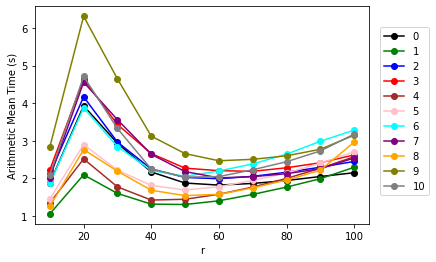
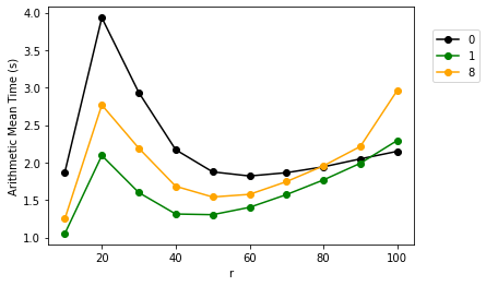
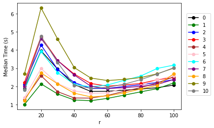
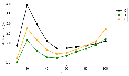
Figure 1: Results for order-3 nonnegative tensors with size $r\times r\times r$ and $n=500$ samples.

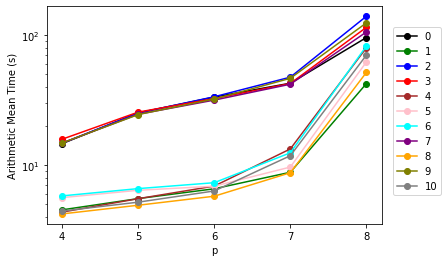
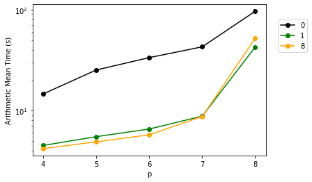
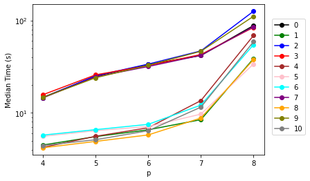
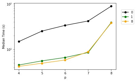
Figure 2: Results for increasing order nonnegative tensors with size $10^{\times p}$ and $n=10,000$ samples.

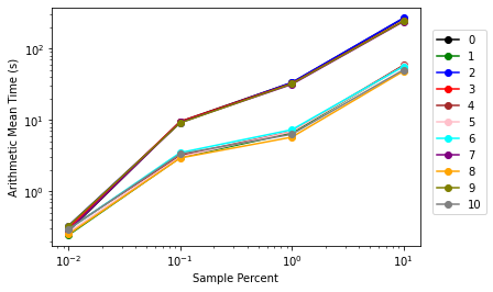
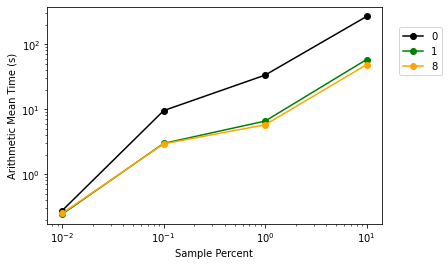
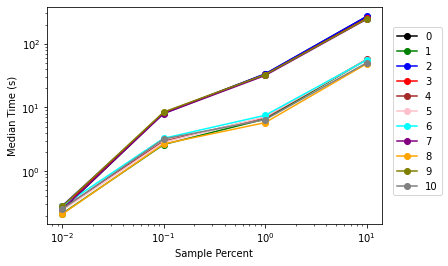
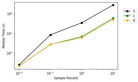
Figure 3: Results for nonnegative tensors with size $10^{\times 6}$ and increasing $n$ samples.

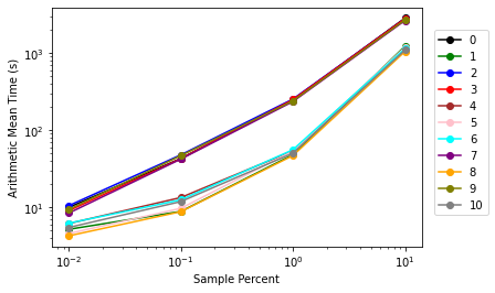
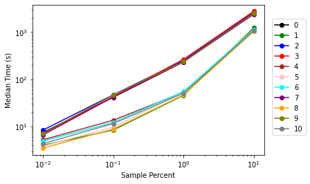
Figure 4: Results for nonnegative tensors with size $10^{\times 7}$ and increasing $n$ samples.

5.5 Technique 4: BPCG

The fifth technique BPCG is for accelerating SiGD. Tsuji et al. [2021] developed the Blended Pairwise Conditional Gradients (BPCG) by combining the Pairwise Conditional Gradients (PCG) with the blending criterion from BCG. Specifically, we applied the lazified version of BPCG, which only differs from BCG by replacing SiGD with PCG.

5.6 Computation Variants

We create ten computational variants of ABCG by mixing the five acceleration techniques described above. They are described in Table LABEL:variants of Appendix 1. There are two observations. First, Index and Pattern are always used together as Pattern relies on Index, so we combine and consider them as a single technique in all following discussions. Second, NAG and BPCG are exclusive to each other as BPCG removes SiGD completely.

6 Numerical Experiments

For benchmarking we adopted the same problem instances (four sets of nonnegative tensor completion problems) and setup as Bugg et al. [2022]. We ran the original algorithm as well as each variant on these instances. The experiments were conducted on a laptop computer with 32GB of RAM and an Intel Core i7 2.2Ghz processor with 6-cores/12-threads. The algorithms were coded in Python 3. Gurobi v9.5.2 [Gurobi Optimization, LLC, 2022] was used to solve the integer programming problem (10). The code is available from https://github.com/WenhaoP/TensorComp. We note that the experiments in Bugg et al. [2022] were conducted using a laptop computer with 8GB of RAM and an Intel Core i5 2.3Ghz processor with 2-cores/4-threads, algorithms coded in Python 3, and Gurobi v9.1 [Gurobi Optimization, LLC, 2022] to solve the integer programming problem (10).

We used NMSE to measure the accuracy and recorded its arithmetic mean (with its standard error) over one hundred repetitions of each problem instance. We recorded the arithmetic mean (with its standard error), geometric mean, minimum, median, and maximum of the computation time over 100 repetitions of each problem instance. Generally speaking, the most effective variants were version 1 (Index + Pattern) and version 8 (BPCG + Index + Pattern), offering consistent speedups over the original version 0 (ABCG). All variants achieve almost the same NMSE as the original algorithm for each problem, which shows that they maintain in practice the same theoretical guarantee as the original algorithm; moreover, their runtimes were mostly competitive with the original.

6.1 Experiments with Order-$3$ Tensors

The first set of problems is order-$3$ tensors with increasing dimensions and $n=500$ samples. The results are in Table LABEL:order3 of Appendix 2, and the arithmetic mean and median computation time is plotted in Figure 2. Among all versions, version 1 (Index + Pattern) has the lowest mean and median computation time for each problem except for the $100\times 100\times 100$ tensor problem, where the original version 0 (ABCG) is slightly faster. Thus, we claim version 1 (Index + Pattern) as the best to use for this set of problems.

6.2 Experiments with Increasing Tensor Order

The second set of problems is tensors with increasing tensor order, with each dimension $r_{i}=10$ for $i=1,\dots,p$, and $n=10,000$ samples. The results are in Table LABEL:inc-order of Appendix 2, and the arithmetic mean and median computation time is plotted in Figure 2. Among all the versions, version 1 (Index + Pattern) and version 8 (BPCG + Index + Pattern) has the lowest mean and median computation time for each problem except for the $10^{\times 8}$ tensor problem. Thus, we claim versions 1 (Index + Pattern) and 8 (BPCG + Index + Pattern) are the best to use for this set of problems.

For the $10^{\times 8}$ tensor problem, version 5 (NAG + Index + Pattern) has the lowest median computation time. We observe that its median computation time is much lower than its mean computation time, and the same occurs with other versions involving NAG. The maximum computation time of these versions is also much higher than other versions. This is due to the fact that, in certain cases, AltMin failed to solve the weak-separation oracle, and the Gurobi solver was needed to solve the time-consuming integer programming problem (10).

6.3 Experiments with Increasing Sample Size

The third and fourth set of problems is tensors of size $10^{\times 6}$ and $10^{\times 7}$ with increasing sample sizes. The results are in Table LABEL:inc-n-1 and Table LABEL:inc-n-2 of Appendix 2, and the arithmetic mean and median computation time is plotted in Figure 4 and 4. Among all the versions, either version 1 (Index + Pattern) or version 8 (BPCG + Index + Pattern) has the lowest mean and median computation time for each problem. Thus, we claim versions 1 (Index + Pattern) and 8 (BPCG + Index + Pattern) are the best to use for this set of problems.

7 Discussion and Conclusion

This paper proposed and evaluated multiple speedup techniques of the original numerical computation algorithm for nonnegative tensor completion created by Bugg et al. [2022]. We benchmarked these algorithm variants on the same set of problem instances designed by Bugg et al. [2022]. Our benchmarking results were that versions 1 (Index + Pattern) and 8 (BPCG + Index + Pattern) generally had the fastest computation time for solving the nonnegative tensor completion problem (6), offering substantial speedups over the original algorithm. Version 1 had Index and Pattern techniques, and version 8 had BPCG, Index, and Pattern techniques. Because version 8 is version 1 with BPCG, version 8 may be preferred over version 1 for problem instances where the active vertex set could be large. Surprisingly, we found that Sparse failed to yield improvements. A possible reason is that the implementation of Sparse needs extra operations (e.g., finding the indices of nonzero entries) for converting NumPy arrays to SciPy sparse arrays. If the active vertex set is not large enough so that extra operations take time as least as the time saved from matrix multiplications of the active vertex set, then we cannot see an improvement. These results suggest that Index and Pattern are the most important for acceleration, and that BCG and BPCG work equally well overall.

Conflict of Interest Statement

The authors declare that the research was conducted in the absence of any commercial or financial relationships that could be construed as a potential conflict of interest.

Author Contributions

WP, AA, and CC contributed to the conception and design of the study. WP did the programming, ran the numerical experiments, analyzed the results, and wrote the first draft of the manuscript. WP, AA, and CC contributed to the manuscript revision, read, and approved the submitted version.

Funding

This material is based upon work partially supported by the NSF under grant CMMI-1847666.

Data Availability Statement

The datasets generated for this study can be found on Gituhub: https://github.com/WenhaoP/TensorComp.

Appendix 1: Table of Variants

Table 1: ABCG and its ten variants

Version	Sparse	NAG	BPCG	Index	Pattern
0 (ABCG)	FALSE	FALSE	FALSE	FALSE	FALSE
1	FALSE	FALSE	FALSE	TRUE	TRUE
2	TRUE	FALSE	FALSE	FALSE	FALSE
3	FALSE	TRUE	FALSE	FALSE	FALSE
4	TRUE	FALSE	FALSE	TRUE	TRUE
5	FALSE	TRUE	FALSE	TRUE	TRUE
6	TRUE	TRUE	FALSE	TRUE	TRUE
7	FALSE	FALSE	TRUE	FALSE	FALSE
8	FALSE	FALSE	TRUE	TRUE	TRUE
9	TRUE	FALSE	TRUE	FALSE	FALSE
10	TRUE	FALSE	TRUE	TRUE	TRUE
Note: True means we implement this technique in this variant, and False means we do not implement this technique in this variant. For example, version 5 implements NAG, Index, and Pattern.

Appendix 2: Tables of Numerical Experiment Results

Table 2: Results for order-$3$ nonnegative tensors with $n=500$ samples

Tensor	Version	NMSE	Time (s)
Size		Arithmetic	Arithmetic	Geometric
		Mean $\pm$ SE	Mean $\pm$ SE	Mean	Min	Median	Max
$10^{\times 3}$	0	0.017 $\pm$ 0.001	1.874 $\pm$ 0.061	1.777	0.756	1.849	3.935
	1	0.017 $\pm$ 0.001	1.054 $\pm$ 0.044	0.966	0.352	1.006	2.688
	2	0.018 $\pm$ 0.001	2.116 $\pm$ 0.071	1.996	0.757	2.102	4.114
	3	0.017 $\pm$ 0.001	2.225 $\pm$ 0.067	2.120	0.885	2.224	4.234
	4	0.018 $\pm$ 0.001	1.346 $\pm$ 0.060	1.218	0.381	1.277	2.998
	5	0.017 $\pm$ 0.001	1.450 $\pm$ 0.056	1.339	0.398	1.386	3.168
	6	0.017 $\pm$ 0.001	1.868 $\pm$ 0.073	1.720	0.520	1.810	4.035
	7	0.017 $\pm$ 0.001	2.014 $\pm$ 0.063	1.914	0.819	2.001	3.383
	8	0.017 $\pm$ 0.001	1.252 $\pm$ 0.054	1.135	0.443	1.211	2.956
	9	0.017 $\pm$ 0.001	2.834 $\pm$ 0.113	2.600	0.829	2.681	5.694
	10	0.017 $\pm$ 0.001	2.093 $\pm$ 0.103	1.828	0.48	1.821	4.795
$20^{\times 3}$	0	0.115 $\pm$ 0.004	3.931 $\pm$ 0.073	3.860	2.086	3.952	6.390
	1	0.115 $\pm$ 0.004	2.094 $\pm$ 0.043	2.046	1.020	2.139	3.314
	2	0.118 $\pm$ 0.004	4.170 $\pm$ 0.078	4.091	1.884	4.272	5.912
	3	0.118 $\pm$ 0.004	4.639 $\pm$ 0.077	4.574	2.955	4.728	7.014
	4	0.118 $\pm$ 0.004	2.518 $\pm$ 0.051	2.459	1.029	2.588	3.625
	5	0.118 $\pm$ 0.004	2.898 $\pm$ 0.051	2.849	1.522	2.980	3.958
	6	0.118 $\pm$ 0.004	3.879 $\pm$ 0.070	3.811	1.999	3.915	5.515
	7	0.114 $\pm$ 0.004	4.561 $\pm$ 0.076	4.497	2.405	4.636	6.781
	8	0.114 $\pm$ 0.004	2.768 $\pm$ 0.049	2.722	1.173	2.742	4.529
	9	0.117 $\pm$ 0.004	6.315 $\pm$ 0.116	6.200	3.526	6.309	9.101
	10	0.117 $\pm$ 0.004	4.712 $\pm$ 0.096	4.602	2.274	4.747	6.609
$30^{\times 3}$	0	0.240 $\pm$ 0.005	2.935 $\pm$ 0.068	2.852	1.547	2.952	4.793
	1	0.240 $\pm$ 0.005	1.600 $\pm$ 0.039	1.551	0.865	1.584	2.488
	2	0.241 $\pm$ 0.005	2.967 $\pm$ 0.077	2.871	1.659	2.931	5.475
	3	0.241 $\pm$ 0.005	3.435 $\pm$ 0.072	3.360	1.818	3.424	5.760
	4	0.241 $\pm$ 0.005	1.774 $\pm$ 0.051	1.705	0.973	1.711	3.659
	5	0.241 $\pm$ 0.005	2.222 $\pm$ 0.053	2.161	1.228	2.160	3.936
	6	0.241 $\pm$ 0.005	2.846 $\pm$ 0.073	2.757	1.600	2.757	5.172
	7	0.240 $\pm$ 0.005	3.561 $\pm$ 0.082	3.467	1.808	3.419	5.874
	8	0.240 $\pm$ 0.005	2.192 $\pm$ 0.058	2.112	1.060	2.142	3.501
	9	0.239 $\pm$ 0.005	4.649 $\pm$ 0.139	4.433	2.079	4.598	8.300
	10	0.239 $\pm$ 0.005	3.328 $\pm$ 0.117	3.112	1.475	3.313	5.927
$40^{\times 3}$	0	0.323 $\pm$ 0.004	2.171 $\pm$ 0.053	2.111	1.377	2.099	4.007
	1	0.323 $\pm$ 0.004	1.314 $\pm$ 0.032	1.279	0.865	1.255	2.528
	2	0.322 $\pm$ 0.004	2.250 $\pm$ 0.053	2.193	1.439	2.214	4.380
	3	0.321 $\pm$ 0.004	2.661 $\pm$ 0.053	2.610	1.723	2.676	4.692
	4	0.322 $\pm$ 0.004	1.423 $\pm$ 0.033	1.389	0.926	1.365	2.847
	5	0.321 $\pm$ 0.004	1.812 $\pm$ 0.036	1.780	1.225	1.755	3.351
	6	0.321 $\pm$ 0.004	2.211 $\pm$ 0.045	2.172	1.546	2.114	4.350
	7	0.321 $\pm$ 0.004	2.641 $\pm$ 0.059	2.577	1.484	2.627	4.666
	8	0.321 $\pm$ 0.004	1.684 $\pm$ 0.042	1.636	0.984	1.626	3.312
	9	0.321 $\pm$ 0.004	3.125 $\pm$ 0.083	3.022	1.911	3.034	5.673
	10	0.321 $\pm$ 0.004	2.248 $\pm$ 0.071	2.151	1.333	2.058	4.529
$50^{\times 3}$	0	0.385 $\pm$ 0.005	1.876 $\pm$ 0.042	1.835	1.327	1.725	3.046
	1	0.385 $\pm$ 0.005	1.305 $\pm$ 0.027	1.281	0.900	1.216	2.289
	2	0.383 $\pm$ 0.004	2.025 $\pm$ 0.045	1.982	1.321	1.885	3.622
	3	0.382 $\pm$ 0.005	2.272 $\pm$ 0.047	2.229	1.676	2.162	3.866
	4	0.383 $\pm$ 0.004	1.444 $\pm$ 0.029	1.418	1.077	1.360	2.535
	5	0.382 $\pm$ 0.005	1.691 $\pm$ 0.032	1.663	1.248	1.618	2.760
	6	0.382 $\pm$ 0.005	2.053 $\pm$ 0.035	2.026	1.566	1.974	3.193
	7	0.384 $\pm$ 0.004	2.181 $\pm$ 0.054	2.121	1.447	2.010	3.839
	8	0.384 $\pm$ 0.004	1.541 $\pm$ 0.038	1.499	1.055	1.425	2.697
	9	0.384 $\pm$ 0.005	2.659 $\pm$ 0.060	2.601	1.889	2.459	4.401
	10	0.384 $\pm$ 0.005	2.033 $\pm$ 0.046	1.989	1.504	1.897	3.544
$60^{\times 3}$	0	0.444 $\pm$ 0.004	1.821 $\pm$ 0.031	1.797	1.409	1.733	2.765
	1	0.444 $\pm$ 0.004	1.403 $\pm$ 0.023	1.386	1.079	1.342	2.154
	2	0.444 $\pm$ 0.004	1.990 $\pm$ 0.033	1.965	1.550	1.887	2.965
	3	0.444 $\pm$ 0.004	2.205 $\pm$ 0.044	2.166	1.565	2.013	3.808
	4	0.444 $\pm$ 0.004	1.577 $\pm$ 0.024	1.560	1.213	1.504	2.348
	5	0.444 $\pm$ 0.004	1.777 $\pm$ 0.031	1.751	1.309	1.641	2.991
	6	0.444 $\pm$ 0.004	2.197 $\pm$ 0.035	2.171	1.626	2.078	3.722
	7	0.445 $\pm$ 0.005	2.013 $\pm$ 0.044	1.970	1.442	1.879	3.631
	8	0.445 $\pm$ 0.005	1.576 $\pm$ 0.032	1.546	1.138	1.478	2.842
	9	0.446 $\pm$ 0.004	2.469 $\pm$ 0.049	2.427	1.791	2.322	4.521
	10	0.446 $\pm$ 0.004	2.047 $\pm$ 0.041	2.012	1.483	1.953	3.967
$70^{\times 3}$	0	0.497 $\pm$ 0.004	1.865 $\pm$ 0.032	1.841	1.386	1.791	3.426
	1	0.497 $\pm$ 0.004	1.573 $\pm$ 0.027	1.552	1.174	1.520	2.861
	2	0.498 $\pm$ 0.004	2.054 $\pm$ 0.032	2.031	1.577	1.995	3.699
	3	0.495 $\pm$ 0.005	2.187 $\pm$ 0.042	2.152	1.548	2.084	4.448
	4	0.498 $\pm$ 0.004	1.768 $\pm$ 0.026	1.751	1.342	1.728	3.095
	5	0.495 $\pm$ 0.005	1.947 $\pm$ 0.036	1.920	1.332	1.895	4.123
	6	0.495 $\pm$ 0.005	2.384 $\pm$ 0.039	2.357	1.689	2.332	4.698
	7	0.498 $\pm$ 0.004	2.045 $\pm$ 0.043	2.006	1.480	1.933	3.964
	8	0.498 $\pm$ 0.004	1.746 $\pm$ 0.037	1.713	1.246	1.640	3.412
	9	0.500 $\pm$ 0.004	2.507 $\pm$ 0.055	2.462	1.891	2.387	5.654
	10	0.500 $\pm$ 0.004	2.229 $\pm$ 0.049	2.190	1.694	2.118	5.11
$80^{\times 3}$	0	0.546 $\pm$ 0.004	1.943 $\pm$ 0.036	1.915	1.439	1.856	3.640
	1	0.546 $\pm$ 0.004	1.768 $\pm$ 0.031	1.743	1.32	1.700	3.273
	2	0.545 $\pm$ 0.004	2.163 $\pm$ 0.035	2.138	1.665	2.092	3.992
	3	0.542 $\pm$ 0.004	2.282 $\pm$ 0.041	2.249	1.654	2.158	3.858
	4	0.545 $\pm$ 0.004	1.998 $\pm$ 0.032	1.976	1.552	1.935	3.759
	5	0.542 $\pm$ 0.004	2.140 $\pm$ 0.037	2.112	1.566	2.043	3.686
	6	0.542 $\pm$ 0.004	2.645 $\pm$ 0.041	2.617	1.959	2.568	4.670
	7	0.547 $\pm$ 0.004	2.125 $\pm$ 0.044	2.087	1.589	2.002	4.312
	8	0.547 $\pm$ 0.004	1.956 $\pm$ 0.043	1.920	1.430	1.859	4.544
	9	0.546 $\pm$ 0.004	2.600 $\pm$ 0.054	2.557	1.902	2.484	6.003
	10	0.546 $\pm$ 0.004	2.443 $\pm$ 0.050	2.405	1.858	2.371	5.699
$90^{\times 3}$	0	0.580 $\pm$ 0.004	2.049 $\pm$ 0.039	2.016	1.416	1.928	3.341
	1	0.580 $\pm$ 0.004	1.991 $\pm$ 0.038	1.959	1.441	1.876	3.380
	2	0.580 $\pm$ 0.004	2.296 $\pm$ 0.036	2.271	1.663	2.216	3.516
	3	0.575 $\pm$ 0.004	2.416 $\pm$ 0.037	2.387	1.669	2.366	3.210
	4	0.580 $\pm$ 0.004	2.269 $\pm$ 0.035	2.244	1.697	2.189	3.367
	5	0.575 $\pm$ 0.004	2.404 $\pm$ 0.038	2.375	1.671	2.367	3.488
	6	0.575 $\pm$ 0.004	2.987 $\pm$ 0.042	2.958	2.101	2.987	4.231
	7	0.579 $\pm$ 0.004	2.257 $\pm$ 0.045	2.216	1.541	2.108	3.658
	8	0.579 $\pm$ 0.004	2.215 $\pm$ 0.045	2.174	1.474	2.062	3.642
	9	0.579 $\pm$ 0.004	2.774 $\pm$ 0.042	2.744	1.854	2.693	4.205
	10	0.579 $\pm$ 0.004	2.729 $\pm$ 0.043	2.698	1.886	2.679	4.089
$100^{\times 3}$	0	0.611 $\pm$ 0.004	2.150 $\pm$ 0.038	2.119	1.520	2.074	3.353
	1	0.611 $\pm$ 0.004	2.295 $\pm$ 0.041	2.262	1.660	2.195	3.702
	2	0.611 $\pm$ 0.004	2.451 $\pm$ 0.037	2.425	1.801	2.373	3.946
	3	0.603 $\pm$ 0.004	2.624 $\pm$ 0.054	2.575	1.671	2.484	4.746
	4	0.611 $\pm$ 0.004	2.575 $\pm$ 0.039	2.547	1.839	2.530	4.168
	5	0.603 $\pm$ 0.004	2.708 $\pm$ 0.054	2.659	1.815	2.589	4.811
	6	0.603 $\pm$ 0.004	3.285 $\pm$ 0.059	3.237	2.173	3.170	5.938
	7	0.608 $\pm$ 0.004	2.542 $\pm$ 0.065	2.468	1.645	2.380	4.636
	8	0.608 $\pm$ 0.004	2.963 $\pm$ 0.097	2.845	1.831	2.698	8.809
	9	0.609 $\pm$ 0.004	3.149 $\pm$ 0.061	3.097	2.128	3.005	6.003
	10	0.609 $\pm$ 0.004	3.178 $\pm$ 0.062	3.126	2.027	3.029	6.136
Note: For each problem, the lowest mean and median computation time are highlighted.

Table 3: Results for increasing order nonnegative tensors and $n=10,000$ samples

Tensor	Version	NMSE	Time (s)
Size		Arithmetic	Arithmetic	Geometric
		Mean $\pm$ SE	Mean $\pm$ SE	Mean	Min	Median	Max
$10^{\times 4}$	0	0.010 $\pm$ 0.000	14.620 $\pm$ 0.160	14.533	11.13	14.723	20.162
	1	0.010 $\pm$ 0.000	4.515 $\pm$ 0.081	4.443	2.658	4.497	7.198
	2	0.010 $\pm$ 0.000	14.736 $\pm$ 0.194	14.622	11.543	14.569	25.271
	3	0.010 $\pm$ 0.000	15.814 $\pm$ 0.194	15.698	11.103	15.732	21.805
	4	0.010 $\pm$ 0.000	4.335 $\pm$ 0.084	4.260	2.725	4.237	8.669
	5	0.010 $\pm$ 0.000	5.608 $\pm$ 0.098	5.521	2.963	5.590	8.890
	6	0.010 $\pm$ 0.000	5.784 $\pm$ 0.107	5.686	2.974	5.752	9.049
	7	0.010 $\pm$ 0.000	14.761 $\pm$ 0.194	14.643	11.197	14.555	22.625
	8	0.010 $\pm$ 0.000	4.200 $\pm$ 0.074	4.138	2.524	4.194	8.091
	9	0.010 $\pm$ 0.000	14.802 $\pm$ 0.199	14.678	10.361	14.700	23.429
	10	0.010 $\pm$ 0.000	4.419 $\pm$ 0.088	4.332	2.424	4.442	8.617
$10^{\times 5}$	0	0.025 $\pm$ 0.001	25.214 $\pm$ 0.275	25.063	18.646	25.012	33.507
	1	0.025 $\pm$ 0.001	5.512 $\pm$ 0.105	5.409	3.140	5.537	8.445
	2	0.025 $\pm$ 0.001	25.195 $\pm$ 0.276	25.041	17.925	25.227	33.771
	3	0.025 $\pm$ 0.001	25.598 $\pm$ 0.275	25.449	18.907	25.801	33.583
	4	0.025 $\pm$ 0.001	5.504 $\pm$ 0.113	5.383	3.106	5.585	8.536
	5	0.025 $\pm$ 0.001	6.391 $\pm$ 0.106	6.297	3.458	6.433	9.155
	6	0.025 $\pm$ 0.001	6.582 $\pm$ 0.109	6.487	3.697	6.590	9.444
	7	0.025 $\pm$ 0.001	24.640 $\pm$ 0.305	24.462	18.711	24.558	39.111
	8	0.025 $\pm$ 0.001	4.899 $\pm$ 0.068	4.850	3.126	4.914	6.599
	9	0.025 $\pm$ 0.001	24.502 $\pm$ 0.290	24.340	17.616	24.007	38.234
	10	0.025 $\pm$ 0.001	5.174 $\pm$ 0.084	5.106	3.203	5.127	8.583
$10^{\times 6}$	0	0.057 $\pm$ 0.002	33.437 $\pm$ 0.475	33.076	17.539	33.360	50.010
	1	0.057 $\pm$ 0.002	6.562 $\pm$ 0.111	6.467	3.647	6.566	9.963
	2	0.058 $\pm$ 0.002	33.606 $\pm$ 0.393	33.357	17.525	33.712	41.967
	3	0.058 $\pm$ 0.003	32.549 $\pm$ 0.436	32.241	18.479	32.502	43.975
	4	0.058 $\pm$ 0.002	6.883 $\pm$ 0.098	6.809	3.914	6.906	8.725
	5	0.058 $\pm$ 0.003	6.869 $\pm$ 0.112	6.770	4.069	7.110	9.002
	6	0.058 $\pm$ 0.003	7.310 $\pm$ 0.121	7.202	4.343	7.522	10.257
	7	0.057 $\pm$ 0.002	31.687 $\pm$ 0.419	31.394	16.671	31.747	42.899
	8	0.057 $\pm$ 0.002	5.750 $\pm$ 0.082	5.688	3.091	5.777	7.923
	9	0.057 $\pm$ 0.003	32.288 $\pm$ 0.399	32.024	18.471	32.798	41.716
	10	0.057 $\pm$ 0.003	6.313 $\pm$ 0.097	6.233	3.326	6.418	8.507
$10^{\times 7}$	0	0.145 $\pm$ 0.007	42.770 $\pm$ 1.192	41.208	15.333	41.701	96.280
	1	0.145 $\pm$ 0.007	8.799 $\pm$ 0.233	8.504	3.763	8.448	17.070
	2	0.147 $\pm$ 0.008	47.611 $\pm$ 1.045	46.352	17.773	46.859	78.931
	3	0.145 $\pm$ 0.008	42.546 $\pm$ 1.046	41.273	18.386	42.818	82.233
	4	0.147 $\pm$ 0.008	13.314 $\pm$ 0.253	13.054	6.425	13.584	19.319
	5	0.145 $\pm$ 0.008	9.650 $\pm$ 0.206	9.430	5.242	9.701	16.758
	6	0.145 $\pm$ 0.008	12.430 $\pm$ 0.254	12.168	6.576	12.144	20.844
	7	0.146 $\pm$ 0.008	41.994 $\pm$ 0.942	40.854	21.795	41.982	60.821
	8	0.146 $\pm$ 0.008	8.729 $\pm$ 0.190	8.522	5.101	8.807	14.279
	9	0.146 $\pm$ 0.008	46.652 $\pm$ 1.067	45.448	21.751	46.404	83.582
	10	0.146 $\pm$ 0.008	11.801 $\pm$ 0.254	11.534	6.208	11.542	20.518
$10^{\times 8}$	0	0.381 $\pm$ 0.021	96.221 $\pm$ 5.042	83.698	15.480	88.210	333.633
	1	0.381 $\pm$ 0.021	42.482 $\pm$ 2.792	36.519	6.272	38.715	254.793
	2	0.387 $\pm$ 0.021	140.427 $\pm$ 10.279	121.552	22.769	125.905	820.344
	3	0.381 $\pm$ 0.021	115.342 $\pm$ 18.396	82.210	14.612	84.227	1690.488
	4	0.387 $\pm$ 0.021	80.225 $\pm$ 7.295	68.880	13.509	68.795	588.859
	5	0.381 $\pm$ 0.021	62.368 $\pm$ 17.093	34.881	6.601	33.880	1589.041
	6	0.380 $\pm$ 0.021	82.748 $\pm$ 14.217	56.711	10.151	54.676	1121.405
	7	0.386 $\pm$ 0.021	106.177 $\pm$ 8.930	86.913	15.541	85.482	678.892
	8	0.386 $\pm$ 0.021	51.834 $\pm$ 7.228	38.044	6.814	37.735	519.459
	9	0.385 $\pm$ 0.021	124.828 $\pm$ 9.714	105.228	19.539	111.054	923.472
	10	0.385 $\pm$ 0.021	70.414 $\pm$ 8.270	57.581	10.774	58.946	837.845
Note: For each problem, the lowest mean and median computation time are highlighted.

Table 4: Results for nonnegative tensors with size $10^{\times 6}$ and increasing $n$ samples

Sample	Version	NMSE	Time (s)
Percent		Arithmetic	Arithmetic	Geometric
		Mean $\pm$ SE	Mean $\pm$ SE	Mean	Min	Median	Max
0.01	0	0.982 $\pm$ 0.004	0.276 $\pm$ 0.010	0.258	0.142	0.246	0.650
	1	0.982 $\pm$ 0.004	0.243 $\pm$ 0.009	0.227	0.122	0.215	0.546
	2	0.981 $\pm$ 0.004	0.329 $\pm$ 0.016	0.298	0.150	0.285	1.019
	3	0.982 $\pm$ 0.004	0.304 $\pm$ 0.012	0.282	0.148	0.265	0.649
	4	0.981 $\pm$ 0.004	0.299 $\pm$ 0.015	0.270	0.130	0.256	0.919
	5	0.982 $\pm$ 0.004	0.265 $\pm$ 0.011	0.246	0.129	0.242	0.576
	6	0.982 $\pm$ 0.004	0.292 $\pm$ 0.013	0.266	0.131	0.281	0.685
	7	0.980 $\pm$ 0.004	0.284 $\pm$ 0.012	0.264	0.151	0.252	0.654
	8	0.980 $\pm$ 0.004	0.250 $\pm$ 0.010	0.232	0.131	0.211	0.549
	9	0.981 $\pm$ 0.004	0.328 $\pm$ 0.016	0.299	0.148	0.281	0.873
	10	0.981 $\pm$ 0.004	0.293 $\pm$ 0.015	0.264	0.129	0.253	0.817
0.1	0	0.564 $\pm$ 0.022	9.507 $\pm$ 0.439	8.565	2.548	8.182	21.995
	1	0.564 $\pm$ 0.022	2.977 $\pm$ 0.116	2.758	0.843	2.616	6.217
	2	0.568 $\pm$ 0.022	9.161 $\pm$ 0.370	8.469	2.804	8.037	20.648
	3	0.571 $\pm$ 0.022	9.504 $\pm$ 0.415	8.647	2.548	8.306	24.41
	4	0.568 $\pm$ 0.022	3.176 $\pm$ 0.107	3.002	1.087	2.948	6.223
	5	0.571 $\pm$ 0.022	3.040 $\pm$ 0.116	2.822	0.874	2.836	7.308
	6	0.571 $\pm$ 0.022	3.482 $\pm$ 0.130	3.237	0.952	3.273	8.053
	7	0.547 $\pm$ 0.023	9.270 $\pm$ 0.467	8.291	2.227	8.018	31.432
	8	0.547 $\pm$ 0.023	2.931 $\pm$ 0.140	2.666	0.844	2.669	10.910
	9	0.562 $\pm$ 0.022	9.111 $\pm$ 0.388	8.329	2.841	8.463	21.631
	10	0.562 $\pm$ 0.022	3.334 $\pm$ 0.129	3.089	0.965	3.194	7.059
1	0	0.057 $\pm$ 0.002	33.437 $\pm$ 0.475	33.076	17.539	33.360	50.010
	1	0.057 $\pm$ 0.002	6.562 $\pm$ 0.111	6.467	3.647	6.566	9.963
	2	0.058 $\pm$ 0.002	33.606 $\pm$ 0.393	33.357	17.525	33.712	41.967
	3	0.058 $\pm$ 0.003	32.549 $\pm$ 0.436	32.241	18.479	32.502	43.975
	4	0.058 $\pm$ 0.002	6.883 $\pm$ 0.098	6.809	3.914	6.906	8.725
	5	0.058 $\pm$ 0.003	6.869 $\pm$ 0.112	6.770	4.069	7.110	9.002
	6	0.058 $\pm$ 0.003	7.310 $\pm$ 0.121	7.202	4.343	7.522	10.257
	7	0.057 $\pm$ 0.002	31.687 $\pm$ 0.419	31.394	16.671	31.747	42.899
	8	0.057 $\pm$ 0.002	5.750 $\pm$ 0.082	5.688	3.091	5.777	7.923
	9	0.057 $\pm$ 0.003	32.288 $\pm$ 0.399	32.024	18.471	32.798	41.716
	10	0.057 $\pm$ 0.003	6.313 $\pm$ 0.097	6.233	3.326	6.418	8.507
10	0	0.050 $\pm$ 0.002	266.905 $\pm$ 3.785	263.971	138.684	266.407	370.278
($n=10^{5}$)	1	0.050 $\pm$ 0.002	58.075 $\pm$ 1.347	56.526	31.177	56.269	101.203
	2	0.051 $\pm$ 0.002	269.866 $\pm$ 3.637	267.083	133.925	268.477	359.523
	3	0.050 $\pm$ 0.002	246.770 $\pm$ 3.353	244.199	138.894	249.96	335.414
	4	0.051 $\pm$ 0.002	58.629 $\pm$ 1.302	57.232	33.940	56.590	93.109
	5	0.050 $\pm$ 0.002	56.653 $\pm$ 0.964	55.822	37.055	56.013	80.008
	6	0.050 $\pm$ 0.002	56.285 $\pm$ 0.975	55.431	34.631	55.497	79.487
	7	0.050 $\pm$ 0.002	241.195 $\pm$ 3.388	238.465	138.051	242.977	333.482
	8	0.050 $\pm$ 0.002	48.434 $\pm$ 0.696	47.934	30.473	48.433	69.063
	9	0.050 $\pm$ 0.002	244.385 $\pm$ 3.051	242.218	149.075	245.842	335.246
	10	0.050 $\pm$ 0.002	50.598 $\pm$ 0.711	50.099	34.797	50.104	73.951
Note: For each problem, the lowest mean and median computation time are highlighted.

Table 5: Results for nonnegative tensors with size $10^{\times 7}$ and increasing $n$ samples

Sample	Version	NMSE	Time (s)
Percent		Arithmetic	Arithmetic	Geometric
		Mean $\pm$ SE	Mean $\pm$ SE	Mean	Min	Median	Max
0.01	0	0.884 $\pm$ 0.016	9.906 $\pm$ 0.733	7.952	1.338	7.456	44.304
	1	0.884 $\pm$ 0.016	5.154 $\pm$ 0.371	4.266	0.772	3.993	25.657
	2	0.883 $\pm$ 0.016	10.435 $\pm$ 0.717	8.677	1.413	8.409	41.956
	3	0.885 $\pm$ 0.015	8.978 $\pm$ 0.637	7.337	1.441	7.069	35.707
	4	0.883 $\pm$ 0.016	6.120 $\pm$ 0.385	5.259	0.897	5.237	25.234
	5	0.885 $\pm$ 0.015	4.542 $\pm$ 0.307	3.846	0.833	3.825	20.304
	6	0.888 $\pm$ 0.015	6.185 $\pm$ 0.496	5.055	0.913	4.931	34.564
	7	0.870 $\pm$ 0.018	8.363 $\pm$ 0.612	6.796	1.506	6.664	40.259
	8	0.870 $\pm$ 0.018	4.242 $\pm$ 0.286	3.585	0.818	3.483	18.221
	9	0.874 $\pm$ 0.017	9.320 $\pm$ 0.663	7.599	1.565	7.122	32.849
	10	0.874 $\pm$ 0.017	5.444 $\pm$ 0.373	4.546	0.939	4.325	21.065
0.1	0	0.145 $\pm$ 0.007	42.770 $\pm$ 1.192	41.208	15.333	41.701	96.280
	1	0.145 $\pm$ 0.007	8.799 $\pm$ 0.233	8.504	3.763	8.448	17.070
	2	0.147 $\pm$ 0.008	47.611 $\pm$ 1.045	46.352	17.773	46.859	78.931
	3	0.145 $\pm$ 0.008	42.546 $\pm$ 1.046	41.273	18.386	42.818	82.233
	4	0.147 $\pm$ 0.008	13.314 $\pm$ 0.253	13.054	6.425	13.584	19.319
	5	0.145 $\pm$ 0.008	9.650 $\pm$ 0.206	9.430	5.242	9.701	16.758
	6	0.145 $\pm$ 0.008	12.430 $\pm$ 0.254	12.168	6.576	12.144	20.844
	7	0.146 $\pm$ 0.008	41.994 $\pm$ 0.942	40.854	21.795	41.982	60.821
	8	0.146 $\pm$ 0.008	8.729 $\pm$ 0.190	8.522	5.101	8.807	14.279
	9	0.146 $\pm$ 0.008	46.652 $\pm$ 1.067	45.448	21.751	46.404	83.582
	10	0.146 $\pm$ 0.008	11.801 $\pm$ 0.254	11.534	6.208	11.542	20.518
1	0	0.112 $\pm$ 0.005	245.863 $\pm$ 6.133	238.338	148.868	233.195	408.085
	1	0.112 $\pm$ 0.005	47.923 $\pm$ 0.899	47.145	32.281	45.655	77.549
	2	0.112 $\pm$ 0.005	252.129 $\pm$ 5.768	245.421	148.470	248.945	366.094
	3	0.113 $\pm$ 0.005	247.820 $\pm$ 5.260	242.007	145.381	264.145	350.913
	4	0.112 $\pm$ 0.005	53.755 $\pm$ 0.978	52.931	35.569	52.759	95.705
	5	0.113 $\pm$ 0.005	53.408 $\pm$ 0.811	52.784	33.295	53.193	73.774
	6	0.113 $\pm$ 0.005	55.586 $\pm$ 0.824	54.963	34.203	55.012	76.677
	7	0.110 $\pm$ 0.005	233.996 $\pm$ 5.571	227.430	143.104	233.493	388.936
	8	0.110 $\pm$ 0.005	46.640 $\pm$ 0.647	46.189	32.440	46.543	64.163
	9	0.109 $\pm$ 0.005	238.510 $\pm$ 5.316	232.407	144.561	235.277	326.239
	10	0.109 $\pm$ 0.005	50.178 $\pm$ 0.679	49.708	34.546	50.580	65.287
10	0	0.108 $\pm$ 0.005	2830.535 $\pm$ 57.672	2773.083	1868.109	2654.533	4015.562
($n=10^{6}$)	1	0.108 $\pm$ 0.005	1223.087 $\pm$ 13.412	1216.033	989.056	1225.745	1662.859
	2	0.108 $\pm$ 0.005	2776.876 $\pm$ 53.723	2726.519	1940.371	2576.609	3907.286
	3	0.110 $\pm$ 0.005	2781.695 $\pm$ 55.039	2728.281	1899.844	2749.232	4377.475
	4	0.108 $\pm$ 0.005	1138.666 $\pm$ 27.790	1117.027	910.320	1065.029	2873.461
	5	0.110 $\pm$ 0.005	1182.486 $\pm$ 19.024	1170.131	939.523	1139.444	2230.349
	6	0.110 $\pm$ 0.005	1137.827 $\pm$ 10.332	1133.184	917.410	1116.388	1408.491
	7	0.108 $\pm$ 0.005	2636.415 $\pm$ 54.039	2583.335	1730.813	2380.683	3738.891
	8	0.108 $\pm$ 0.005	1045.224 $\pm$ 8.729	1041.659	899.932	1032.678	1261.093
	9	0.110 $\pm$ 0.005	2687.159 $\pm$ 50.578	2640.935	1957.054	2510.885	3761.409
	10	0.110 $\pm$ 0.005	1090.345 $\pm$ 8.418	1087.132	928.105	1076.160	1310.540
Note: For each problem, the lowest mean and median computation time are highlighted.

References

- Aswani [2016] Aswani, A. (2016). Low-rank approximation and completion of positive tensors. SIAM Journal on Matrix Analysis and Applications 37, 1337–1364
- Barak and Moitra [2016] Barak, B. and Moitra, A. (2016). Noisy tensor completion via the sum-of-squares hierarchy. In Conference on Learning Theory (PMLR), 417–445
- Besançon et al. [2022] Besançon, M., Carderera, A., and Pokutta, S. (2022). Frankwolfe. jl: A high-performance and flexible toolbox for frank–wolfe algorithms and conditional gradients. INFORMS Journal on Computing
- Braun et al. [2019] Braun, G., Pokutta, S., Tu, D., and Wright, S. (2019). Blended conditonal gradients. In International Conference on Machine Learning (PMLR), 735–743
- Bugg et al. [2022] Bugg, C. X., Chen, C., and Aswani, A. (2022). Nonnegative tensor completion via integer optimization. In Advances in Neural Information Processing Systems, eds. A. H. Oh, A. Agarwal, D. Belgrave, and K. Cho
- Chandrasekaran et al. [2012] Chandrasekaran, V., Recht, B., Parrilo, P. A., and Willsky, A. S. (2012). The convex geometry of linear inverse problems. Foundations of Computational mathematics 12, 805–849
- Gandy et al. [2011] Gandy, S., Recht, B., and Yamada, I. (2011). Tensor completion and low-n-rank tensor recovery via convex optimization. Inverse problems 27, 025010
- Gurobi Optimization, LLC [2022] Gurobi Optimization, LLC (2022). Gurobi optimizer reference manual
- Hansen [1979] Hansen, P. (1979). Methods of nonlinear 0-1 programming. In Annals of Discrete Mathematics (Elsevier), vol. 5. 53–70
- Harris et al. [2020] Harris, C. R., Millman, K. J., Van Der Walt, S. J., Gommers, R., Virtanen, P., Cournapeau, D., et al. (2020). Array programming with numpy. Nature 585, 357–362
- Hillar and Lim [2013] Hillar, C. J. and Lim, L.-H. (2013). Most tensor problems are np-hard. Journal of the ACM (JACM) 60, 1–39
- Kolda and Bader [2009] Kolda, T. G. and Bader, B. W. (2009). Tensor decompositions and applications. SIAM review 51, 455–500
- Lecué [2013] Lecué, G. (2013). Empirical risk minimization is optimal for the convex aggregation problem. Bernoulli 19, 2153–2166
- Liu et al. [2013] Liu, J., Musialski, P., Wonka, P., and Ye, J. (2013). Tensor completion for estimating missing values in visual data. IEEE Transactions on Pattern Analysis and Machine Intelligence 35, 208–220. 10.1109/TPAMI.2012.39
- Montanari and Sun [2018] Montanari, A. and Sun, N. (2018). Spectral algorithms for tensor completion. Communications on Pure and Applied Mathematics 71, 2381–2425
- Mu et al. [2014] Mu, C., Huang, B., Wright, J., and Goldfarb, D. (2014). Square deal: Lower bounds and improved relaxations for tensor recovery. In International conference on machine learning (PMLR), 73–81
- Nemirovski [2000] Nemirovski, A. (2000). Topics in non-parametric statistics. Lectures on probability theory and statistics (Saint-Flour, 1998) 1738, 85–277
- Padberg [1989] Padberg, M. (1989). The boolean quadric polytope: some characteristics, facets and relatives. Mathematical programming 45, 139–172
- Rao et al. [2015] Rao, N., Shah, P., and Wright, S. (2015). Forward–backward greedy algorithms for atomic norm regularization. IEEE Transactions on Signal Processing 63, 5798–5811
- Rauhut and Stojanac [2021] Rauhut, H. and Stojanac, Ž. (2021). Tensor theta norms and low rank recovery. Numerical Algorithms 88, 25–66
- Song et al. [2019] Song, Q., Ge, H., Caverlee, J., and Hu, X. (2019). Tensor completion algorithms in big data analytics. ACM Trans. Knowl. Discov. Data 13. 10.1145/3278607
- Tan et al. [2013] Tan, H., Wu, Y., Feng, G., Wang, W., and Ran, B. (2013). A new traffic prediction method based on dynamic tensor completion. Procedia-Social and Behavioral Sciences 96, 2431–2442
- Tsuji et al. [2021] Tsuji, K., Tanaka, K., and Pokutta, S. (2021). Sparser kernel herding with pairwise conditional gradients without swap steps. arXiv preprint arXiv:2110.12650
- Tsybakov [2003] Tsybakov, A. B. (2003). Optimal rates of aggregation. In Learning theory and kernel machines (Springer). 303–313
- Virtanen et al. [2020] Virtanen, P., Gommers, R., Oliphant, T. E., Haberland, M., Reddy, T., Cournapeau, D., et al. (2020). Scipy 1.0: fundamental algorithms for scientific computing in python. Nature methods 17, 261–272
- Yuan and Zhang [2016] Yuan, M. and Zhang, C.-H. (2016). On tensor completion via nuclear norm minimization. Foundations of Computational Mathematics 16, 1031–1068
- Yuan and Zhang [2017] Yuan, M. and Zhang, C.-H. (2017). Incoherent tensor norms and their applications in higher order tensor completion. IEEE Transactions on Information Theory 63, 6753–6766
- Zhang et al. [2019] Zhang, X., Wang, D., Zhou, Z., and Ma, Y. (2019). Robust low-rank tensor recovery with rectification and alignment. IEEE Transactions on Pattern Analysis and Machine Intelligence 43, 238–255