Graphical models for infinite measures
with applications to extremes and Lévy processes

Abstract

Conditional independence and graphical models are well studied for probability distributions on product spaces. We propose a new notion of conditional independence for any measure $\Lambda$ on the punctured Euclidean space $\mathbb{R}^{d}\setminus\{0\}$ that explodes at the origin. The importance of such measures stems from their connection to infinitely divisible and max-infinitely divisible distributions, where they appear as Lévy measures and exponent measures, respectively. We characterize independence and conditional independence for $\Lambda$ in various ways through kernels and factorization of a modified density, including a Hammersley-Clifford type theorem for undirected graphical models. As opposed to the classical conditional independence, our notion is intimately connected to the support of the measure $\Lambda$. Our general theory unifies and extends recent approaches to graphical modeling in the fields of extreme value analysis and Lévy processes. Our results for the corresponding undirected and directed graphical models lay the foundation for new statistical methodology in these areas.

, and

1 Introduction

Conditional independence is a central concept in probability theory that enables the definition of graphical models and the notion of sparsity. It is the backbone of modern statistical methodology for understanding latent structures in the data, construction of parsimonious models in high dimensions and estimation of causal relationships (Dawid, 1979; Maathuis et al., 2019; Lauritzen, 1996). The classical notion of probabilistic conditional independence is defined for random vectors through factorizations of conditional probabilities. In fact, following an axiomatic approach, conditional independence can be seen as a more general notion of irrelevance with applications beyond random vectors (e.g., Lauritzen, 1996, Chapter 3).

In this paper we define a new notion of conditional independence and graphical models for the class of Borel measures $\Lambda$ on the punctured $d$-dimensional Euclidean space $\mathcal{E}=\mathbb{R}^{d}\setminus\{0\}$, where $\Lambda$ is finite on all Borel sets that are bounded away from the origin. For disjoint subsets $A,B,C$ of the index set $V=\{1,\dots,d\}$, we denote this conditional independence of $A$ and $B$ given $C$ for the measure $\Lambda$ by

$$A\perp B\mid C\;[\Lambda].$$ (1)

The essence of our definition in Section 3.2 is that we require classical conditional independence on the normalized restrictions of $\Lambda$ to any charged product form set in $\mathcal{E}$ that is bounded away from the origin.

Measures $\Lambda$ of the above kind are indeed fundamental in various fields of probability and statistics. Notably, they arise as Lévy measures of infinitely divisible probability laws with respect to semi-group operations on $\mathbb{R}^{d}$ for which the origin is a neutral element (Berg, Christensen and Ressel, 1984). We focus here on the following important examples. A random vector $X$ is (sum-)infinitely divisible or max-infinitely divisible, if for every $n\in\mathbb{N}$ it has the stochastic representation

$$X\stackrel{{\scriptstyle d}}{{=}}\sum_{i=1}^{n}X^{(n,i)},\quad\text{or}\quad X\stackrel{{\scriptstyle d}}{{=}}\bigvee_{i=1}^{n}X^{(n,i)},$$ (2)

respectively, for some independent, identically distributed vectors $X^{(n,1)},\ldots,X^{(n,n)}$, where the sums and maxima are taken in the component-wise sense. In the context of maxima, the term exponent measure is often preferred over Lévy measure for $\Lambda$ and we adopt the same convention here (Resnick, 2008). Importantly, infinitely divisible distributions appear as limit laws of triangular arrays; for sums this observation dates back to Skorohod (1957) and Feller (1971, Part XVII.11), for instance, and we refer to Balkema and Resnick (1977) and de Haan and Resnick (1977) for maxima. This explains the ubiquity of measures $\Lambda$ and their appearance in the vast literature on related point processes, random sets or large deviation principles (e.g., Dombry and Ribatet, 2015; Hult and Lindskog, 2007; Davydov, Molchanov and Zuyev, 2008). In most situations, including typical cases of sum- and max-infinitely divisible distributions, the measure $\Lambda$ explodes at the origin and therefore has infinite mass on $\mathcal{E}$. Therefore, classical probabilistic conditional independence is not meaningful for such measures. Our new notion in (1) resolves this issue in an arguably natural way.

A first fundamental result for our new conditional independence is that, under a mild explosiveness assumption, the four axioms of a semi-graphoid are satisfied (Lauritzen, 1996, Chapter 3). This directly implies various useful properties of the corresponding graphical models. Moreover, we provide several alternative characterizations. If $\Lambda$ possesses a density $\lambda$ with respect to some product measure, then the conditional independence (1) is equivalent to the factorization of (a modified version of) this density. Under the mild explosiveness condition, (1) induces certain constraints on the support of the measure $\Lambda$. In particular, the independence $A\perp B\;[\Lambda]$ is completely characterized by the condition that $\Lambda$ can have mass only on certain sub-faces of $\mathcal{E}$. This is in sharp contrast to usual probabilistic independence, which would suggest a factorization of the measure into the product of marginals. Graphical models for measures $\Lambda$ as above can be defined readily by means of suitable Markov properties. We reveal several fundamental links between properties of the measure $\Lambda$ and the graph structure. For instance, for an undirected, decomposable graph we prove a Hammersley–Clifford type theorem that states that the global Markov property for $\Lambda$ is equivalent to a factorization of the modified density of $\Lambda$ on the cliques of the graph.

The general theory of conditional independence and graphical models for $\Lambda$ measures translates into new insights in the respective areas of probability theory, where such measures arise naturally. In particular, many of our findings in this manuscript have been motivated by recent developments and open questions from multivariate extreme value theory, which studies the dependence structure in the distributional tail of a random vector. The most fundamental limiting models that appear in this field are max-stable distributions, which are max-infinitely divisible distributions with homogeneous exponent measures $\Lambda$, that is,

$$\Lambda(tA)=t^{-{\alpha}}\Lambda(A),\qquad t>0,$$ (3)

for some $\alpha>0$ and all Borel sets $A\subset\mathcal{E}$ bounded away from the origin. While classical theory in this field intensively studied stochastic processes with spatial domains (e.g., de Haan, 1984; Kabluchko, Schlather and de Haan, 2009), recent research concentrates on finding sparse structures in multivariate extreme value models; see Engelke and Ivanovs (2021) for an overview. One line of work develops recursive max-linear models on directed acyclic graphs, which correspond to a specific class of spectrally discrete max-stable distributions (Gissibl and Klüppelberg, 2018; Klüppelberg and Lauritzen, 2019). However, if a max-stable distribution admits a positive density, it cannot satisfy non-trivial (classical) conditional independence (Papastathopoulos and Strokorb, 2016). Instead, Engelke and Hitz (2020) define a notion of extremal conditional independence and undirected graphical models on the level of multivariate Pareto distributions (Rootzén and Tajvidi, 2006), which can also be characterized by the homogeneous exponent measure $\Lambda$; see Section 8.1 for details. In the case of tree graphs, these models arise as extremal limits of regularly varying Markov trees (Segers, 2020).

These two active research directions have so far co-existed without a clear connection. Since max-linear models and multivariate Pareto distributions are both described by the exponent measure $\Lambda$, it seems natural that this object also encodes the graphical properties. Indeed, it turns out that our conditional independence notion in (1) unifies and extends both approaches. We show that for recursive max-linear models, any classical conditional independence implied by its directed acyclic graph is also present on the level of $\Lambda$ in the sense of (1). Concerning the extremal conditional independence in Engelke and Hitz (2020), we note that it is originally only defined if $\Lambda$ has a Lebesgue density on $\mathcal{E}$ and no mass on sub-faces. As a consequence, no extremal independence can exist and their extremal graphical models are always connected. Several discussion contributions of their paper raised these points as limitations for statistical modeling. Our conditional independence (1) extends the notion of Engelke and Hitz (2020) to arbitrary exponent measures $\Lambda$ and thereby overcomes several of these restrictions.

1. It allows for disconnected extremal graphs with mass on sub-faces and, as an illustration, we provide an extension of Hüsler–Reiss tree models (Engelke and Volgushev, 2020; Asenova, Mazo and Segers, 2021) to forests with richer dependence structures. Since no densities are required, our notion also includes max-linear models.

2. It extends to max-infinitely divisible distributions that can exhibit asymptotic independence (Huser, Opitz and Thibaud, 2021), and therefore opens the door to graphical modeling in this large field of research, in which many approaches go back to the conditional approach for extreme value modelling by Heffernan and Tawn (2004).

3. The support constraints from the conditional independence of $\Lambda$ connect our theory to sparsity notions for tails of multivariate distributions and the field of concomitant extremes (e.g., Chiapino and Sabourin, 2017).

We discuss these extensions in Section 8 and provide some basic examples that motivate the potential for the construction of new models. A more in-depth study of these new modelling routes and the development of corresponding statistical methodology is beyond the scope of this paper.

Another promising application of our theory lies in the field of infinitely divisible distributions and Lévy processes (Ivanovs, 2020), where $\Lambda$ plays the role of the Lévy measure. Much less literature on graphical models and sparsity exists in this area. In the case of $\alpha$-stable distributions, that is, if the Lévy measure is homogeneous as in (3), Misra and Kuruoglu (2016) introduce recursive stable models that are similar to Gissibl and Klüppelberg (2018). Again, the classical conditional independence is reflected in the corresponding (degenerate) Lévy measure $\Lambda$ through our conditional independence. For more general Lévy measures, we can define graphical models with respect to our $\Lambda$-based notion of conditional independence. We provide an outlook on how this translates into probabilistic properties of the corresponding Lévy processes in the concluding Section 9; the details of this direction are part of future research.

2 Preliminaries

2.1 Conditional independence

Consider a probability space $(\Omega,\mathcal{A},\mathbb{P})$ and let $X,Y,Z$ be random elements with values in some Borel spaces. Conditional independence of $X$ and $Y$ given $Z$ with respect to $\mathbb{P}$, denoted by

$$X\perp\!\!\!\perp Y\mid Z,$$

is defined as the factorization of conditional probabilities

$$\mathbb{P}(X\in E_{X},Y\in E_{Y}|Z)=\mathbb{P}(X\in E_{X}|Z)\mathbb{P}(Y\in E_{Y}|Z),\qquad\text{a.s.},$$

for all $E_{X},E_{Y}$ in the respective $\sigma$-algebras; we refer to Kallenberg (2002, Chapter 6) for the basic theory and further properties. In terms of the regular conditional probability $\mathbb{P}(\cdot|Z=z)$ it reads

$$\mathbb{P}(X\in E_{X},Y\in E_{Y}|Z=z)=\mathbb{P}(X\in E_{X}|Z=z)\mathbb{P}(Y\in E_{Y}|Z=z),\quad\text{ for }\mathbb{P}_{Z}\text{-almost all }z,$$

where $\mathbb{P}_{Z}$ denotes the law of $Z$. By a standard argument (see Kallenberg, 2002, Thm. 6.3), this factorization holds for all such $E_{X},E_{Y}$ and all $z$ outside some fixed $\mathbb{P}_{Z}$-null set. In other words, $X$ and $Y$ are independent under $\mathbb{P}(\cdot|Z=z)$ for $\mathbb{P}_{Z}$-almost all $z$.

In the situation, when $(X,Y,Z)$ possesses a joint density $f(x,y,z)$ with respect to some product measure $\mu=\mu_{X}\otimes\mu_{Y}\otimes\mu_{Z}$, where each component is a $\sigma$-finite measure, the conditional independence $X\perp\!\!\!\perp Y\mid Z$ is equivalent to the following density decomposition:

$$f(x,y,z)f_{Z}(z)=f_{XZ}(x,z)f_{YZ}(y,z)\qquad\text{ for }\mu\text{-almost all }(x,y,z),$$

using the naturally induced notation for the marginal densities; see for instance Dawid (1979) or Lauritzen (1996, Chapter 3). In particular, if $(X,Y,Z)$ is discrete, then its probability mass function factorizes for all $(x,y,z)$. If $\mu$ is Lebesgue and all the involved densities are continuous, then this equality must be true for all $(x,y,z)$. Note that continuity of $f$ does not imply continuity of the marginal densities, which explains the formulation of the last sentence.

2.2 Infinitely divisible distributions for sums and maxima

For $d\geq 1$ consider the domain $\mathcal{E}=\mathbb{R}^{d}\setminus\{0\}$, which is a $d$-dimensional space of real numbers punctured at the origin. Let $\Lambda$ be a Borel measure on this domain, such that the following basic boundedness condition is satisfied:

$$\Lambda(A)<\infty\qquad\text{for any Borel set }A\subset\mathcal{E}\text{ bounded away from the origin}.$$ (B)

As discussed in the introduction, such measures appear naturally in various areas of probability and statistics. In particular, they arise in the limits of sums and maxima of random variables in the theory of infinitely divisible and max-infinitely divisible distributions as in (2).

In the max-infinitely divisible case we assume that each component $X_{j}$ is non-negative with lower endpoint $0$, that is, each $X_{j}$ has some mass arbitrarily close to 0:

$$\quad\inf\{x:\mathbb{P}(X_{j}\leq x)>0\}=0.$$ (4)

Then the distribution function of $X$ is given by

$$\mathbb{P}(X\leq x)=\exp\big{[}-\Lambda(\mathcal{E}_{+}\setminus[0,x])\big{]},\qquad x\geq 0,$$ (5)

where $\Lambda$ is null outside of the domain $\mathcal{E}_{+}=[0,\infty)^{d}\setminus\{0\}$ and satisfies (B), while $x\geq 0$ is meant componentwise; see Resnick (2008, Prop. 5.8). Conversely, every such measure $\Lambda$, called an exponent measure, leads to a max-infinitely divisible distribution. The standard assumption $\Lambda(\mathcal{E}_{+})=\infty$ corresponds to no point mass of $X$ at the origin. One may also define a Poisson point process with intensity measure $\mathrm{d}t\otimes\Lambda(\mathrm{d}x)$ and retrieve $X$ as the maximum over the space-points with $t\leq 1$.

In the infinitely divisible case the characteristic function of $X$ is given by

$$\mathbb{E}e^{{\rm i}\left\langle\theta,X\right\rangle}=\exp\bigg{[}-\frac{1}{2}\left\langle\theta,\Sigma\theta\right\rangle+{\rm i}\left\langle\gamma,\theta\right\rangle+\int_{\mathcal{E}}\big{(}e^{{\rm i}\left\langle\theta,x\right\rangle}-1-{\rm i}\left\langle\theta,x\right\rangle\mbox{\rm\large 1}_{\{{\|x\|}\leq 1\}}\big{)}\Lambda(\mathrm{d}x)\bigg{]},\,\,\theta\in\mathbb{R}^{d},$$

where $\gamma\in\mathbb{R}^{d}$ is a drift parameter, $\Sigma$ is the symmetric, non-negative definite $d\times d$ covariance matrix of the Gaussian component, and $\Lambda$ is the so-called Lévy measure, which satisfies (B) together with $\int_{{\|x\|}\in(0,1)}{\|x\|}^{2}\Lambda(\mathrm{d}x)<\infty$, where ${\|\cdot\|}$ is an arbitrary norm on $\mathbb{R}^{d}$; see Sato (2013, Thm. 8.1). The Lévy measure is used to define a Poisson point process of jumps with intensity measure $\mathrm{d}t\otimes\Lambda(\mathrm{d}x)$, the compensated sum of which yields the non-Gaussian part of $X$ in the limit sense. Conversely, every such characteristic triplet $(\gamma,\Sigma,\Lambda)$ leads to an infinitely divisible law.

Example 2.1.

Let $\Phi_{\rho}:\mathbb{R}^{2}\to[0,1]$ be the distribution function of a bivariate normal distribution with correlation coefficient $\rho\in[0,1]$ and standard normal margins. When $\rho>0$, the bivariate normal distribution is max-infinitely divisible (Resnick, 2008, Section 5.2), a property inherited by the corresponding log-normal distribution $\Phi_{\rho}\circ\log$. Thus, by (5)

$$\Lambda_{\rho}(\mathcal{E}_{+}\setminus[0,x])=-\log\Phi_{\rho}(\log x),\quad x\geq 0,$$

is a valid measure satisfying (B). In addition, it explodes at the origin.

Various connections between the infinitely divisible and max-infinitely divisible laws have been explored in Kabluchko (2009) and Wang and Stoev (2010). Davydov, Molchanov and Zuyev (2008) and Molchanov (2009) draw further attention to multivariate $\ell_{p}$-infinitely divisible laws, or more generally, infinitely divisible laws with respect to semi-group operations. All of these works focus on the important special case where the involved Lévy measures (or exponent measures) $\Lambda$ are $-{\alpha}$-homogeneous, that is, the property (3) holds for some $\alpha>0$. A max-infinitely divisible $X$ with (standard) ${\alpha}$-Fréchet marginals is max-stable if and only if $\Lambda$ is $-{\alpha}$-homogeneous (Resnick, 2008, Prop. 5.11). An infinitely divisible $X$ is ${\alpha}$-stable with ${\alpha}\in(0,2)$ if and only if $\Sigma=0$ and $\Lambda$ is $-{\alpha}$-homogeneous (Sato, 2013, Thm. 14.3(ii)).

Example 2.2.

The exponent measure corresponding to the bivariate max-stable Hüsler–Reiss distributions (Hüsler and Reiss, 1989) with parameter $\Gamma>0$ is

$$\Lambda_{\Gamma}(\mathcal{E}_{+}\setminus[0,x])=-\frac{1}{x_{1}}\Phi\left(\frac{\sqrt{\Gamma}}{2}+\frac{\log(x_{2}/x_{1})}{\sqrt{\Gamma}}\right)-\frac{1}{x_{2}}\Phi\left(\frac{\sqrt{\Gamma}}{2}+\frac{\log(x_{1}/x_{2})}{\sqrt{\Gamma}}\right),\quad x\geq 0,$$

where $\Phi$ denotes the univariate standard normal distribution function. This measure also satisfies (B). Since it is $-1$-homogeneous, it also explodes at the origin.

3 Definition of conditional independence for $\Lambda$ and first properties

3.1 Setup and notation

As previously, let $V=\{1,\ldots,d\}$ be a finite index set and $\Lambda$ a measure on $\mathcal{E}=\mathbb{R}^{V}\setminus\{0_{V}\}$ satisfying (B). For a subset $A\subset\mathcal{E}$, we say that a property holds for $\Lambda$-almost all $y\in A$ if the subset of $A$ where it does not hold is a $\Lambda$-null set. As test sets for conditional independence we consider the class $\mathcal{R}(\Lambda)$ of charged product-form sets in $\mathcal{E}$ not containing the origin $0_{V}$ in their closure

$$\mathcal{R}(\Lambda)=\bigg{\{}R=\bigtimes_{v\in V}R_{v}\,:\,R_{v}\in\mathcal{B}(\mathbb{R}),\,\Lambda(R)>0,\,0_{V}\notin\overline{R}\bigg{\}}.$$ (6)

By definition, we have $\Lambda(R)\in(0,\infty)$ for any $R\in\mathcal{R}(\Lambda)$, which allows us to define a probability measure $\mathbb{P}_{R}$ on $R$ via

$$\mathbb{P}_{R}(\mathrm{d}y)=\frac{\Lambda(\mathrm{d}y)}{\Lambda(R)}.$$ (7)

We write $Y\sim\mathbb{P}_{R}$ for a $d$-dimensional random vector $Y$ distributed according to $\mathbb{P}_{R}$.

For a non-empty subset $D$ of $V$, the measure $\Lambda$ induces two natural measures on the lower dimensional domain

$$\mathcal{E}^{D}=\mathbb{R}^{D}\setminus\{0_{D}\},$$

namely the marginal measure $\Lambda_{D}$ and the restricted measure $\Lambda_{D}^{0}$ as given by

$$\Lambda_{D}(\cdot)=\Lambda(y_{D}\in\cdot), \Lambda_{D}^{0}(\cdot)=\Lambda(y_{D}\in\cdot\,,\,y_{V\setminus D}=0_{V\setminus D}),$$ (8)

respectively. Both measures also satisfy the basic assumption (B) in their common domain $\mathcal{E}^{D}$.

The class $\mathcal{R}(\Lambda_{D})$ is understood to contain product form sets $R_{D}=\bigtimes_{d\in D}R_{d}$ (satisfying the other conditions as in (6) with respect to $\mathbb{R}^{D}$ instead of $\mathbb{R}^{V}$) and the respective probability measures are denoted by $\mathbb{P}_{R_{D}}$. The product set $R$ will sometimes be written as $R_{D}\times R_{V\setminus D}$ irrespective of the indices in $D$. Note that $R_{D}\in\mathcal{R}(\Lambda_{D})$ implies $R_{D}\times\mathbb{R}^{V\setminus D}\in\mathcal{R}(\Lambda)$. Some basic consistency properties are stated in Appendix A.1.

3.2 Definition of conditional independence for $\Lambda$

We are now ready to give our definition of conditional independence for the measure $\Lambda$ based on the above test sets.

Definition 3.1.

For disjoint sets $A,B,C\subset V$ that form a partition of $V$, we say that $\Lambda$ admits conditional independence of $A$ and $B$ given $C$, denoted by

$$A\perp B\mid C\;[\Lambda],$$

if we have the classical conditional independence

$$Y_{A}\perp\!\!\!\perp Y_{B}\mid Y_{C}\qquad\text{for }\quad Y\sim\mathbb{P}_{R}\quad\text{ for all }\quad R\in\mathcal{R}(\Lambda).$$ (9)

This is trivially true for $A$ or $B$ being empty, and for $C=\emptyset$ we say that $\Lambda$ admits independence of $A$ and $B$, and write

$$A\perp B\;[\Lambda].$$

If the sets $A,B$ and $C$ are not a partition of $V$, then the above definition remains the same with the test class in (9) replaced by $\mathcal{R}(\Lambda_{A\cup B\cup C})$.

Remark 3.2.

If $\Lambda$ is a zero measure, the test classes $\mathcal{R}(\Lambda_{A\cup B\cup C})$ are empty, hence any such (conditional) independence statement with respect to $\Lambda$ is true. Moreover, for strictly monotone, continuous transformations $T_{v}:\mathbb{R}\to\mathbb{R}$ with $T_{v}(0)=0$, $v\in V$, the conditional independence of $\Lambda$ in Definition 3.1 is equivalent to the corresponding statement for the pushforward measure $\Lambda\circ T^{-1}$ for $T(x)=(T_{v}(x_{v}))_{v\in V}$. Definition 3.1 is similar to the notion of conditional inner independence as suggested by Zhang and Wang (2020) for a random vector supported by a non-product-form space.

It is useful to observe that for $A\cup B\cup C\subset D\subset V$, the two statements

$$A\perp B\mid C\;[\Lambda]\qquad\text{and}\qquad A\perp B\mid C\;[\Lambda_{D}]$$ (10)

are equivalent. However, some caution is needed. We would like to stress that the conditional independence $A\perp B\mid C\;[\Lambda]$ does not(!) imply

$$Y_{A}\perp\!\!\!\perp Y_{B}\mid Y_{C}\qquad\text{for }\quad Y\sim\mathbb{P}_{R}\quad\text{ for all }\quad R\in\mathcal{R}(\Lambda)$$

unless $(A,B,C)$ is a partition of $V$, because restriction according to the additional dimensions in $V\setminus(A\cup B\cup C)$ amounts to conditioning on the respective components; see Lemma A.2 in Appendix A.1.

A second simple observation, which will accompany us throughout this work, is the following:

Lemma 3.3.

$A\perp B\mid C\;[\Lambda]$ implies $A\perp B\,[\Lambda^{0}_{A\cup B}]$.

Proof.

If $\Lambda^{0}_{A\cup B}$ is null, there is nothing to prove. Else consider $R_{A\cup B}\in\mathcal{R}(\Lambda^{0}_{A\cup B})$ and the respective $Y_{A\cup B}$. Set $Y_{C}=0_{C}$ and note that the law of such a vector $Y$ alternatively arises from the measure $\Lambda$ and the set $R_{A\cup B}\times\{0_{C}\}\in\mathcal{R}(\Lambda)$. Now $A\perp B\mid C\;[\Lambda]$ implies $Y_{A}\perp\!\!\!\perp Y_{B}\mid Y_{C}$ and thus also $Y_{A}\perp\!\!\!\perp Y_{B}$, because $Y_{C}=0_{C}$ a.s. ∎

Remark 3.4.

Slightly more general, the same reasoning shows that $A\perp B\mid C\;[\Lambda]$ implies $A\perp B\,|\,C^{\prime}\,[\Lambda^{0}_{A\cup B\cup C^{\prime}}]$ for any subset $C^{\prime}\subset C$. When $C=\emptyset$, the statement in Lemma 3.3 is a tautology.

3.3 Semi-graphoid properties

A semi-graphoid is an abstract independence model that satisfies a set of algebraic properties (Pearl, 1988; Lauritzen, 1996; Maathuis et al., 2019). For our conditional independence defined in Section 3.2 for a measure $\Lambda$, if $A,B,C,D$ are disjoint subsets of $V$, these properties read as follows.

• If $A\perp B\,|\,C\,[\Lambda]$, then $B\perp A\,|\,C\,[\Lambda]$. (Symmetry)

• If $A\perp(B\cup D)\,|\,C\,[\Lambda]$, then $A\perp B\,|\,C\,[\Lambda]$. (Decomposition)

• If $A\perp(B\cup D)\,|\,C\,[\Lambda]$, then $A\perp B\,|\,C\cup D\,[\Lambda]$. (Weak union)

• If $A\perp B\,|\,C\,[\Lambda]$ and $A\perp D\,|\,B\cup C\,[\Lambda]$, then $A\perp(B\cup D)\,|\,C\,[\Lambda]$. (Contraction)

These conditions are crucial in the study of graphical models as they directly imply certain equivalences or implications among fundamental Markov properties usually considered in directed and undirected graphical models; see Sections 6 and 7.

If we restrict our attention to homogeneous measures $\Lambda$ that admit a Lebesgue density on $\mathcal{E}_{+}$ as considered in Engelke and Hitz (2020) in the context of extreme value theory, Steffen Lauritzen argues already in his discussion contribution that their extremal conditional independence is a semi-graphoid. We will confirm this finding below. However, our general setting here goes far beyond this situation in several ways. Our $\Lambda$ is not necessarily homogeneous, it does not necessarily have a density, its mass is not restricted to the positive upper orthant and it may even have mass on sub-faces of $\mathcal{E}$. This leads to a situation, where only the properties (L1)–(L3) always hold. The contraction condition (L4) is more involved.

Proposition 3.5.

Conditional independence with respect to $\Lambda$ as defined in Definition 3.1 satisfies (L1), (L2) and (L3).

Proof.

Properties (L1) and (L3) follow directly from their respective counterparts for probability laws, whereas (L2) follows similarly if one takes into account the compatibility with marginal measures as stated in Lemma A.2. ∎

It will be shown in Theorem 5.3 below that also property (L4) is true under the explosiveness assumption (E1). This property is not true, however, for general finite measures $\Lambda$, in which case our Definition 3.1 might not be natural. The problem arises from the exclusion of the origin in the domain $\mathcal{E}=\mathbb{R}^{V}\setminus\{0_{V}\}$, which is neither necessary nor natural in the finite case. The following simple example illustrates this.

Example 3.6 (Violation of (L4) for a finite measure).

Consider $A=\{1\},B=\{2\},C=\emptyset,D=\{3\}$ and $\Lambda$ putting mass 1 at each of the points $(0,0,1)$ and $(1,1,1)$; see Figure 1 for an illustration. Observe that $\Lambda_{A\cup B}$ is a point mass at $(1,1)$ and so we trivially have $A\perp B\;[\Lambda]$. Furthermore, we also have $A\perp D\mid B\;[\Lambda]$, because the two point masses have a different $B$ coordinate and so any admissible $\mathbb{P}_{R}$ results in the corresponding conditional independence statement. Finally, the statement $A\perp(B\cup D)\;[\Lambda]$ is not true, because there exists a product set, namely $R=\mathbb{R}\times\mathbb{R}\times\{1\}$, for which we get that $Y\sim\mathbb{P}_{R}$ can only assume the values $(0,0,1)$ or $(1,1,1)$, each with probability $1/2$, and thus, $Y_{1}$ and $(Y_{2},Y_{3})$ are not independent.

Figure 1: Illustration of Example 3.6. The measure $\Lambda$ consists of two point masses with different $y_{2}$-coordinate, so that $\{1\}\perp\{3\}\mid\{2\}~{}[\Lambda]$ (center). Its marginal measure $\Lambda_{12}$ is a point mass (right), hence $\{1\}\perp\{2\}~{}[\Lambda]$. However, the restriction of $\Lambda$ to the admissible product set $\mathbb{R}\times\mathbb{R}\times\{1\}$ does not factorize (left); the L4 conclusion $\{1\}\perp\{2,3\}~{}[\Lambda]$ is violated.

4 Alternative characterizations of $\Lambda$-conditional independence

We establish three alternative characterizations of the conditional independence $A\perp B\mid C\;[\Lambda]$ in this section, each of which further demonstrates that our notion is both natural and intuitive. The first characterization, Theorem 4.1, is a reduction to test sets of a simple form. The second, Theorem 4.4, is in terms of the underlying probability (Markov) kernel $\nu(y_{C},\cdot)$ from $\mathcal{E}^{C}$ to $\mathbb{R}^{A\cup B}$. It allows to view our notion of conditional independence as the classical independence for a family of probability laws. The third, Theorem 4.6, is in terms of the factorization of the density of $\Lambda$ with respect to some dominating measure, assuming it exists.

Without loss of generality, we focus on the case, where the sets $A$, $B$ and $C$ form a partition of $V$. The independence case $C=\emptyset$ is excluded, unless mentioned otherwise, but we return to it in Section 5. The more technical proofs and auxiliary results are given in Appendix A.

4.1 Reduction of the test class

Our first result reduces the test class $\mathcal{R}=\mathcal{R}(\Lambda)$ to sets of the form

$$R_{v,{\varepsilon}}=\{y\in\mathbb{R}^{d}:|y_{v}|\geq{\varepsilon}\}=(\mathbb{R}\setminus(-{\varepsilon},{\varepsilon}))^{\{v\}}\times\mathbb{R}^{V\setminus\{v\}},\qquad v\in V,\,{\varepsilon}>0.$$ (11)

When writing $Y\sim\mathbb{P}_{R_{v,{\varepsilon}}}$, we implicitly assume $\Lambda(R_{v,{\varepsilon}})>0$ and hence $R_{v,{\varepsilon}}\in\mathcal{R}(\Lambda)$. The proof is postponed to Appendix A.

Theorem 4.1 (CI via test classes).

Let $(A,B,C)$ be a partition of $V$. Then $A\perp B\mid C\;[\Lambda]$ is equivalent to any of the following statements:

1. $Y_{A}\perp\!\!\!\perp Y_{B}\mid Y_{C}$ with $Y\sim\mathbb{P}_{R_{v,{\varepsilon}}}$ for all $v\in V,\,{\varepsilon}>0$,

2. $Y_{A}\perp\!\!\!\perp Y_{B}\mid Y_{C}$ with $Y\sim\mathbb{P}_{R_{c,{\varepsilon}}}$ for all $c\in C,\,{\varepsilon}>0$, and additionally, $A\perp B\;[\Lambda^{0}_{A\cup B}]$.

Moreover, $A\perp B\;[\Lambda]$ is equivalent to (i) with $C=\emptyset$.

Remark 4.2.

The characterizations (i) and (ii) in Theorem 4.1 can be modified in various ways. For instance in item (i) a single $v\in V$ is sufficient when $\Lambda^{0}_{V\setminus\{v\}}$ is a zero measure; see Lemma A.7 below. If the measure $\Lambda$ is homogeneous, it suffices to consider a fixed ${\varepsilon}>0$ instead of all ${\varepsilon}>0$, e.g., ${\varepsilon}=1$.

4.2 Probability kernel

We verify first that the measure $\Lambda$ can be represented in terms of a probability kernel (Kallenberg, 2002, p. 20) when restricted to the set $\{y\in\mathcal{E}:y_{C}\neq 0\}$. To this end we use the notation that a set $R$ is of product form if it can be represented as $R=\bigtimes_{v\in V}R_{v}=R_{A\cup B}\times R_{C}$ with $R_{v}\in\mathcal{B}(\mathbb{R})$ and $0_{C}\not\in R_{C}$. We postpone the technical proof to Appendix A.

Lemma 4.3 (Probability kernel representation).

There exists a $\Lambda_{C}$-unique probability kernel $\nu_{C}$ from $\mathcal{E}^{C}$ to $\mathbb{R}^{A\cup B}$ such that for all $R$ of product form we have

$$\Lambda(R)=\int_{y_{C}\in R_{C}}\nu_{C}(y_{C},R_{A\cup B})\Lambda_{C}(\mathrm{d}y_{C})\in[0,\infty],\qquad\text{if }0_{C}\notin R_{C}.$$

Moreover, for any $c\in C$ and ${\varepsilon}>0$ such that $\Lambda(R_{c,{\varepsilon}})>0$ there is the identity

$$\nu_{C}(y_{C},R_{A\cup B})=\mathbb{P}(Y_{A\cup B}\in R_{A\cup B}|Y_{C}=y_{C}),\qquad Y\sim\mathbb{P}_{R_{c,{\varepsilon}}}$$

for $\Lambda_{C}$-almost all $y_{C}$ with $|y_{c}|\geq{\varepsilon}$.

We can now characterize conditional independence as given by Definition 3.1 in terms of this kernel representation.

Theorem 4.4 (CI via kernel factorization).

Let $(A,B,C)$ be a partition of $V$. Then $A\perp B\mid C\;[\Lambda]$ if and only if the probability kernel factorizes,

$$\nu_{C}(y_{C},R_{A\cup B})=\nu_{C}(y_{C},R_{A}\times\mathbb{R}^{B})\nu_{C}(y_{C},R_{B}\times\mathbb{R}^{A})$$

for $\Lambda_{C}$-almost all $y_{C}\neq 0_{C}$ and any $R_{A\cup B}$ of product form, and additionally $A\perp B\;[\Lambda_{A\cup B}^{0}]$.

Proof.

According to Theorem 4.1 (ii) it is sufficient to show that $Y_{A}\perp\!\!\!\perp Y_{B}\mid Y_{C}$ with $Y\sim\mathbb{P}_{R_{c,{\varepsilon}}}$ for all $c\in C,\,{\varepsilon}>0$ if and only if the kernel factorizes for $\Lambda_{C}$-almost all $y_{C}\neq 0_{C}$. Fix $c\in C,\,{\varepsilon}>0$ and note that $Y_{A}\perp\!\!\!\perp Y_{B}\mid Y_{C}$ is equivalent to

$$\mathbb{P}(Y_{A\cup B}\in R_{A\cup B}|Y_{C}=y_{C})=\mathbb{P}(Y_{A}\in R_{A}|Y_{C}=y_{C})\mathbb{P}(Y_{B}\in R_{B}|Y_{C}=y_{C})$$

for $\mathbb{P}_{Y_{C}}$-almost all $y_{C}$ and any product form $R_{A\cup B}$. These are $\Lambda_{C}$-almost all $y_{C}$ satisfying $|y_{c}|\geq{\varepsilon}$ and the factorization can be stated in terms of the kernel $\nu_{C}$ according to its representation in Lemma 4.3. This factorization readily extends to $\Lambda_{C}$-almost all $y_{C}\neq 0_{C}$, since $c\in C,\,{\varepsilon}>0$ are arbitrary, which completes the proof. ∎

4.3 Density factorization

An important case concerns the measure $\Lambda$ having density $\lambda$ on $\mathcal{E}$ with respect to some product measure

$$\mu=\bigotimes_{v\in V}\mu_{v},$$

where each $\mu_{v}$ is a $\sigma$-finite measure on $(\mathbb{R},\mathcal{B}(\mathbb{R}))$. For any non-empty $D\subset V$, the marginal density $\lambda_{D}$, the density of $\Lambda_{D}$ in (8), with respect to $\mu_{D}=\bigotimes_{v\in D}\mu_{v}$ is

$$\lambda_{D}(y_{D})=\int\lambda(y_{D},y_{V\setminus D})\mu_{V\setminus D}(\mathrm{d}y_{V\setminus D}),\qquad y_{D}\neq 0_{D},$$

which must be finite for $\mu_{D}$-almost all $y_{D}\neq 0_{D}$. We also note that the density $\lambda^{0}_{D}$ of $\Lambda_{D}^{0}$ with respect to $\mu_{D}$ is given by

$$\lambda^{0}_{D}(y_{D})=\lambda(y_{D},0_{V\setminus D})\mu_{V\setminus D}(\{0_{V\setminus D}\}),\qquad y_{D}\neq 0_{D}.$$

Lemma 4.5 (Kernel density).

Assume that $\Lambda$ has a $\mu$-density $\lambda$. Then the probability kernel $\nu(y_{C},\cdot)$ has density

$$f_{y_{C}}(y_{A\cup B})=\frac{\lambda(y)}{\lambda_{C}(y_{C})}$$

with respect to $\mu_{A\cup B}$ for $\Lambda_{C}$-almost all $y_{C}\neq 0_{C}$.

Proof.

Take any $R$ of product form such that $0_{C}\notin R_{C}$, and observe that

$$\Lambda(R)=\int_{y_{C}\in R_{C}}\Big{(}\int_{y_{A\cup B}\in R_{A\cup B}}\frac{\lambda(y)}{\lambda_{C}(y_{C})}\mu_{A\cup B}(\mathrm{d}y_{A\cup B})\Big{)}\Lambda_{C}(\mathrm{d}y_{C}).$$

Hence the expression in brackets coincides with $\nu(y_{C},R_{A\cup B})$ for all $R_{A\cup B}$ and $\Lambda_{C}$-all $y_{C}\neq 0_{C}$, see Lemma 4.3. ∎

This readily yields another characterization result of our conditional independence (Definition 3.1 with $C\neq\emptyset$).

Theorem 4.6 (CI via density factorization).

Let $(A,B,C)$ be a partition of $V$ and assume that $\Lambda$ has a $\mu$-density $\lambda$. Then $A\perp B\mid C\;[\Lambda]$ if and only if the factorization

$$\lambda(y)\lambda_{C}(y_{C})=\lambda_{A\cup C}(y_{A\cup C})\lambda_{B\cup C}(y_{B\cup C})$$

holds for $\mu$-almost all $y\in\mathcal{E},\,y_{C}\neq 0_{C}$, and additionally, $A\perp B\;[\Lambda^{0}_{A\cup B}]$.

Proof.

According to Theorem 4.4 it will suffice to establish equivalence to the kernel factorization. By Lemma 4.5 kernel factorization is equivalent to $\mu_{A\cup B}$-almost everywhere factorization of the density $f_{y_{C}}$ for $\Lambda_{C}$-almost all $y_{C}\neq 0_{C}$. The marginal density of $f_{y_{C}}$ with respect to $A$ is given by $\lambda_{A\cup C}(y_{A\cup C})/\lambda_{C}(y_{C})$ and the analogous result holds for the set $B$. Thus, we have

$$\frac{\lambda(y)}{\lambda_{C}(y_{C})}=\frac{\lambda_{A\cup C}(y_{A\cup C})}{\lambda_{C}(y_{C})}\,\frac{\lambda_{B\cup C}(y_{B\cup C})}{\lambda_{C}(y_{C})}$$

for $\mu_{A\cup B}\otimes\Lambda_{C}$-almost all $(y_{A\cup B},y_{C})$ with $y_{C}\neq 0_{C}$. It is left to note that the set $\{y:\lambda_{C}(y_{C})=0,\lambda_{A\cup C}(y_{A\cup C})>0\}$ is $\mu$-negligible. ∎

Importantly, we do not claim that the independence statement $A\perp B\;[\Lambda]$ implies the factorization $\lambda(y)=\lambda_{A}(y_{A})\lambda_{B}(y_{B})$. The marginals $\lambda_{A}$ and $\lambda_{B}$ are not even defined for $y_{A}=0_{A}$ or $y_{B}=0_{B}$, respectively, and considering a restriction to $y_{A}\neq 0_{A}$, $y_{B}\neq 0_{B}$ does not resolve the matter either; see Section 5.3 below. Instead, as will be also shown in Section 5.3, one needs to consider a modified density in order to achieve an equivalence to a (modified) density factorization.

5 Independence and the support of $\Lambda$

5.1 Independence characterization via the support of $\Lambda$

Throughout this section we make the following explosiveness assumption

$$\Lambda\big{(}y_{v}\neq 0\big{)}\in\{0,\infty\}\qquad\text{for all }v\in V,$$ (E0)

which means that all one-dimensional marginal measures of $\Lambda$ are either infinite or zero measures.

Proposition 5.1 (Independence).

Consider a partition $(A,B)$ of $V$ and assume (E0). Then

$$A\perp B\;[\Lambda]\qquad\iff\qquad\Lambda(y_{A}\neq 0_{A}\text{ and }\,y_{B}\neq 0_{B})=0.$$

Proof.

The if statement follows trivially from the definition, since every admissible $Y$ is such that either $Y_{A}=0_{A}$ a.s. or $Y_{B}=0_{B}$ a.s. (the assumption (E0) is not needed for this direction).

Now assume $A\perp B\;[\Lambda]$ and that the support of $\Lambda$ contains some $y$ with $y_{a}\neq 0$ and $y_{b}\neq 0$ for some $a\in A$, $b\in B$. Note that $\Lambda_{\{a\}}$ is infinite by (E0), since it can not be a zero measure. Furthermore, we may take $\delta>0$ small such that $\Lambda(R_{a,\delta}\cap R_{b,\delta})>0$. Letting $Y\sim\Lambda(R_{a,{\varepsilon}})$ with ${\varepsilon}\in(0,\delta)$ we observe that

$$\frac{\Lambda(R_{a,\delta}\cap R_{b,\delta})}{\Lambda(R_{a,{\varepsilon}})}=\mathbb{P}(|Y_{a}|\geq\delta,|Y_{b}|\geq\delta)=\mathbb{P}(|Y_{a}|\geq\delta)\mathbb{P}(|Y_{b}|\geq\delta)=\frac{\Lambda(R_{a,\delta})}{\Lambda(R_{a,{\varepsilon}})}\frac{\Lambda(R_{b,\delta}\cap R_{a,{\varepsilon}})}{\Lambda(R_{a,{\varepsilon}})}.$$

Multiply both sides by $\Lambda(R_{a,{\varepsilon}})\in(0,\infty)$ and observe that $\Lambda(R_{b,\delta}\cap R_{a,{\varepsilon}})$ stays bounded, whereas $\Lambda(R_{a,{\varepsilon}})\to\Lambda(y_{a}\neq 0)=\infty$ as ${\varepsilon}\downarrow 0$. Hence $\Lambda(R_{a,\delta}\cap R_{b,\delta})=0$, a contradiction. ∎

Proposition 5.1 is closely related to the concept of asymptotic independence in extremes, which we discuss in Section 8. We may rephrase the condition in Proposition 5.1 in a number of ways, for instance in terms of the sets

$$\mathcal{H}_{D}=\{y\in\mathcal{E}\,:\,y_{V\setminus D}=0_{V\setminus D}\}=\bigcup_{\emptyset\neq A\subset D}\mathcal{E}_{A},$$ (12)

where $\mathcal{E}_{A}=\{y\in\mathcal{E}\,:\,y_{i}\neq 0\,\,\forall\,i\in A\,\text{ and }\,y_{i}=0\,\forall\,i\notin A\}$ is the sub-face of $\mathcal{E}$ corresponding to the subset $A\subset V$; it should not be confused with $\mathcal{E}^{A}=\mathbb{R}^{A}\setminus\{0_{A}\}$. For convenience we summarize a few of these reformulations as follows. Figure 2 provides an illustration.

Corollary 5.2.

Consider a partition $(A,B)$ of $V$ and assume (E0). The following statements are equivalent.

1. $A\perp B\;[\Lambda]$

2. $\Lambda(\mathcal{E}^{A}\times\mathcal{E}^{B})=\Lambda(y_{A}\neq 0_{A}\text{ and }\,y_{B}\neq 0_{B})=0$

3. ${\rm supp}(\Lambda)\subset\mathcal{H}_{A}\cup\mathcal{H}_{B}$

4. $\Lambda_{A}=\Lambda_{A}^{0}$

5. $\Lambda_{B}=\Lambda_{B}^{0}$

The independence characterization of Proposition 5.1 (or its extended reformulation Corollary 5.2) only treats the case where $(A,B)$ is a partition of $V$. Suppose that this is not the case and denote by $(A,B,C)$ a partition of $V$. We recall that by (10), $A\perp B\;[\Lambda]$ is equivalent to $A\perp B\;[\Lambda_{A\cup B}]$ and that (E0) for $\Lambda$ implies (E0) for $\Lambda_{A\cup B}$. Thus, applying Proposition 5.1 to the measure $\Lambda_{A\cup B}$, we obtain

$$A\perp B\;[\Lambda]\,\,\,\,\iff\,\,\,\,\Lambda(y_{A}\neq 0_{A},\,y_{B}\neq 0_{B})=0\,\,\,\,\iff\,\,\,\,{\rm supp}(\Lambda)\subset\mathcal{H}_{A\cup C}\cup\mathcal{H}_{B\cup C}.$$ (13)

Due to Lemma 3.3, we will often work with the statement $A\perp B\;[\Lambda^{0}_{A\cup B}]$. If (E0) holds for the reduced measure $\Lambda^{0}_{A\cup B}$, Proposition 5.1 translates into the equivalence

$$A\perp B\;[\Lambda^{0}_{A\cup B}]\quad \iff\quad\Lambda(y_{A}\neq 0_{A},\,y_{B}\neq 0_{B},\,y_{C}=0_{C})=0$$

$$\iff\quad{\rm supp}(\Lambda)\subset\mathcal{H}_{A}\cup\mathcal{H}_{B}\cup(\mathcal{E}\setminus\mathcal{H}_{A\cup B}).$$

When translating items (iv) and (v) from Corollary 5.2 to these situations, where $A$ and $B$ are not a partition of $V$, but only disjoint, it is useful to take Lemma A.1 from Appendix A.1 into account.

     

Figure 2: Illustration of the sets $\mathcal{H}_{D}$ for $V=\{1,2,3\}$. No mass of $\Lambda$ outside of $\mathcal{H}_{\{1,2\}}$ and $\mathcal{H}_{\{3\}}$ corresponds to $\{1,2\}\perp\{3\}\;[\Lambda]$, see Proposition 5.1. No mass of $\Lambda$ outside of $\mathcal{H}_{\{1,2\}}$ and $\mathcal{H}_{\{2,3\}}$ corresponds to $\{1\}\perp\{3\}\;[\Lambda]$, see (13).

5.2 Contraction semi-graphoid property (L4)

We are now in a position to establish the remaining contraction semi-graphoid property (L4). In order to do so, we need to strengthen the explosiveness assumption (E0), so that it also holds for all underlying restricted measures:

$$\Lambda^{0}_{D}(y_{d}\neq 0)\in\{0,\infty\}\qquad\text{for all }d\in D\subset V.$$ (E1)

Assumption (E1) means that all one-dimensional marginals of all restricted measures $\Lambda^{0}_{D}$ (including $\Lambda=\Lambda^{0}_{V}$) are either infinite or zero measures. This necessarily entails that also all one-dimensional marginals of all marginal measures $\Lambda_{D}$ are infinite or zero measures.

Theorem 5.3.

Under Assumption (E1) conditional independence with respect to $\Lambda$ as defined in Definition 3.1 satisfies all four semi-graphoid properties (L1)–(L4).

Proof.

Properties (L1)–(L3) are already established in Proposition 3.5. To prove (L4), it is sufficient to assume that the union of $A,B,C,D$ is $V$; see Lemma A.2.

First we establish (L4) for $C=\emptyset$. That is, we show that for a partition $(A,B,D)$ of $V$ the statements $A\perp B\;[\Lambda]$ and $A\perp D\mid B\;[\Lambda]$ imply $A\perp B\cup D\;[\Lambda]$. According to Proposition 5.1 we need to show that $\Lambda$ has no mass outside of $\mathcal{H}_{A}\cup\mathcal{H}_{B\cup D}$. Note that $A\perp B\;[\Lambda]$ implies that there is no mass outside of $\mathcal{H}_{A\cup D}\cup\mathcal{H}_{B\cup D}$, whereas $A\perp D\mid B\;[\Lambda]$ implies $A\perp D\;[\Lambda^{0}_{A\cup D}]$, see Lemma 3.3, and thus all the mass of $\Lambda$ on $\mathcal{H}_{A\cup D}$ must be contained in $\mathcal{H}_{A}\cup\mathcal{H}_{D}$. Summarizing, ${\rm supp}({\Lambda})\subset(\mathcal{H}_{A}\cup\mathcal{H}_{D})\cup\mathcal{H}_{B\cup D}=\mathcal{H}_{A}\cup\mathcal{H}_{B\cup D}$, completing the first part of the proof. Here we used the explosiveness assumption (E0) for the measures $\Lambda_{A\cup B}$ and $\Lambda^{0}_{A\cup D}$, which follows from (E1).

Finally we prove the case $C\neq\emptyset$. As a consequence of Lemma 3.3 and Lemma A.1 we see that $A\perp B\mid C\;[\Lambda]$ implies $A\perp B\;[\Lambda^{0}_{A\cup B\cup D}]$, whereas $A\perp D\,|\,B\cup C\,[\Lambda]$ implies $A\perp D\,|\,B\,[\Lambda^{0}_{A\cup B\cup D}]$ (see Remark 3.4). Hence from the first step we readily get $A\perp(B\cup D)\,[\Lambda^{0}_{A\cup B\cup D}]$. According to Theorem 4.1 (ii) it is left to consider $Y\sim\mathbb{P}_{R_{c,{\varepsilon}}}$ for $c\in C$, ${\varepsilon}>0$, and to establish $Y_{A}\perp\!\!\!\perp Y_{B\cup D}\mid Y_{C}$. But the assumption in (L4) implies $Y_{A}\perp\!\!\!\perp Y_{B}\mid Y_{C}$ (see Lemma A.2) and $Y_{A}\perp\!\!\!\perp Y_{D}\mid Y_{B\cup C}$, and we apply the classical analogue of (L4) to complete the proof. ∎

Remark 5.4.

At first sight, the explosiveness assumption (E1) may seem restrictive. However, it is a very natural condition for exponent measures and Lévy measures in the context of infinitely divisible distributions; see Section 2.2. Importantly, for a $-\alpha$-homogeneous $\Lambda$ as in (3), all measures $\Lambda^{0}_{D}$ are $-\alpha$-homogeneous and so Assumption (E1) is satisfied. In addition, the necessity of this assumption (see Example 3.6) underlines the special role of the origin in our setting, which is not apparent through the first three properties (L1)–(L3).

5.3 A modified density

Here we revisit the case when $\Lambda$ has a density $\lambda$ with respect to a product measure $\mu=\bigotimes_{v\in V}\mu_{v}$. Let us first review the independence situation. Under assumption (E0) the independence $A\perp B\;[\Lambda]$ is equivalent to $\Lambda(y_{A}\neq 0_{A},y_{B}\neq 0_{B})=0$. In this case

$$\lambda_{D}(y_{D}) =\lambda_{D}^{0}(y_{D}), \text{for $\mu_{D}$-almost all }y_{D}\in\mathcal{E}^{D}\text{ for }D\in\{A,B\},$$

whereas $\lambda(y)=0$ for $\mu$-almost all $y=(y_{A},y_{B})\in\mathcal{E}^{A}\times\mathcal{E}^{B}$. So, unless we have the degenerate situation that the full measure $\Lambda$ is entirely concentrated either on $\mathcal{H}_{A}$ only or on $\mathcal{H}_{B}$ only, a factorization of the form $\lambda(y)=\lambda_{A}(y_{A})\lambda_{B}(y_{B})$ for $\mu$-almost all $y\in\mathcal{E}^{A}\times\mathcal{E}^{B}$ cannot hold true. Hence the density does not factorize on the product set where the marginals are defined.

However, with a slight modification of the density, we can achieve a factorization, as long it is tested only on the correct subsets of $\mathbb{R}^{V}$. To this end, we will assume $\mu_{v}(\{0_{v}\})>0$ for all $v\in V$, and we define for a non-empty $D\subset V$ the modified densities

$$\overline{\lambda}_{D}(y_{D})=\begin{cases}\lambda_{D}(y_{D})&\text{for }y_{D}\in\mathcal{E}^{D}=\mathbb{R}^{D}\setminus\{0_{D}\},\\ 1/\mu_{D}(\{0_{D}\})&\text{for }y_{D}=0_{D},\end{cases}$$ (14)

whereas $\overline{\lambda}_{\emptyset}=1$. As a special case of the following result we will see that $A\perp B\;[\Lambda]$ is equivalent to the factorization

$$\overline{\lambda}(y)=\overline{\lambda}_{A}(y_{A})\overline{\lambda}_{B}(y_{B})$$

for $\mu$-almost all $y\in\mathcal{E}$ with either $y_{A}=0_{A}$ or $y_{B}=0_{B}$.

Proposition 5.5.

Assume (E1) and that $\Lambda$ has a $\mu$-density $\lambda$, where $\mu_{v}(\{0_{v}\})>0$ for all $v\in V$. Then for a partition $(A,B,C)$ of $V$ with possibly empty $C$ the conditional independence $A\perp B\mid C\;[\Lambda]$ is equivalent to the factorization

$$\overline{\lambda}(y)\overline{\lambda}_{C}(y_{C})=\overline{\lambda}_{A\cup C}(y_{A\cup C})\overline{\lambda}_{B\cup C}(y_{B\cup C})$$

for $\mu$-almost all $y\in\mathbb{R}^{V}\setminus\{y:y_{A}\neq 0_{A},y_{B}\neq 0_{B},y_{C}=0_{C}\}$.

Proof.

For $y=0_{V}$ the statement is trivial; it follows simply from the factorization of $\mu(\{0_{V}\})$ into the factors $\mu_{v}(\{0_{v}\})$, $v\in V$. On the set $\{y_{C}\neq 0_{C}\}$ this factorization is that of $\lambda$. In view of Theorem 4.6 it is sufficient to check that $A\perp B\;[\Lambda^{0}_{A\cup B}]$ is equivalent to the factorization of $\overline{\lambda}$ for $\mu$-almost all $y\neq 0$ with $y_{A\cup C}=0_{A\cup C}$ or $y_{B\cup C}=0_{B\cup C}$.

Indeed, according to Corollary 5.2 the independence $A\perp B\;[\Lambda^{0}_{A\cup B}]$ is equivalent to $\Lambda(y_{A}\neq 0_{A},y_{B}\neq 0_{B},y_{C}=0_{C})=0$, which holds if and only if

$$\lambda_{A\cup C}(y_{A\cup C})=\lambda_{A}^{0}(y_{A})/\mu_{C}(\{0_{C}\}) =\lambda(y)\mu_{B}(\{0_{B}\})$$ (15)

for $\mu$-almost all $y\neq 0$ with $y_{B\cup C}=0_{B\cup C}$, and the analogous statement with exchanged roles of $A$ and $B$ holds. The equality (15) can be rewritten as

$$\lambda(y)/\mu_{C}(\{0_{C}\})=\lambda_{A\cup C}(y_{A\cup C})/\mu_{B\cup C}(\{0_{B\cup C}\}),$$

which is the claimed factorization of $\overline{\lambda}$ on $\{y\in\mathcal{E}:y_{B\cup C}=0_{B\cup C}\}$. The same argument applies with roles of $A$ and $B$ interchanged, and the proof is complete. ∎

Remark 5.6.

If $A\perp B\mid C\;[\Lambda]$, then $\Lambda(\{y:y_{A}\neq 0_{A},y_{B}\neq 0_{B},y_{C}=0_{C}\})=0$. Proposition 5.5 does not need the entire extended explosiveness assumption (E1). It is sufficient to assume (E0) for the reduced measure $\Lambda^{0}_{A\cup B}$ instead, which is guaranteed by (E1).

5.4 A generic construction

To conclude this section we give a constructive example of a measure $\Lambda$ in $d=3$ dimensions with index set $V=\{1,2,3\}$ such that the conditional independence $\{1\}\perp\{3\}\mid\{2\}\;[\Lambda]$ holds. As a dominating product measure $\mu$ we take

$$\mu(\mathrm{d}x_{1},\ldots,\mathrm{d}x_{d})=\bigotimes_{i=1}^{d}\mu_{i}(\mathrm{d}x_{i})=\bigotimes_{i=1}^{d}(\mathrm{d}x_{i}+\delta_{0}(\mathrm{d}x_{i})),$$ (16)

where $\delta_{0}$ is the point mass at 0. As building blocks, we employ two bivariate densities $\kappa_{ij}$ for $(i,j)\in\{(1,2),(2,3)\}$ defined on $(0,\infty)^{2}$ with identical univariate marginal densities $\kappa_{i}(y_{i})=m(y_{i})$, $y_{i}\in(0,\infty)$, for all $i\in V$. As in (B) we further assume that the marginal measure on $(0,\infty)$ defined by the density $m$ puts finite mass on sets bounded away from 0. For each of these bivariate densities $\kappa_{ij}$ we can add mass on the axes to define a density with respect to the measure $\mu_{ij}=\mu_{i}\otimes\mu_{j}$ on $\mathcal{E}_{+}^{ij}=[0,\infty)^{\{i,j\}}\setminus\{0_{\{i,j\}}\}$ by

$$\lambda_{ij}(y_{ij})=p_{ij}\mbox{\rm\large 1}_{\{y_{i},y_{j}\neq 0\}}\kappa_{ij}(y_{ij})+q_{ij}\mbox{\rm\large 1}_{\{y_{j}=0\}}m(y_{i})+q_{ij}\mbox{\rm\large 1}_{\{y_{i}=0\}}m(y_{j}),\quad y_{ij}\in\mathcal{E}_{+}^{ij},$$ (17)

where $p_{ij}\in[0,1]$ is a mixture probability and $q_{ij}=1-p_{ij}$; the case $p_{ij}=0$ implies independence between components $i$ and $j$ in the sense of Proposition 5.1.

By construction, the marginal densities of $\lambda_{ij}$ also satisfy $\lambda_{i}(y_{i})=m(y_{i})$ for $i\in V$. We can combine these two bivariate densities using the modified densities in (14) into a trivariate density

$$\lambda(y)=\overline{\lambda}_{12}(y_{12})\overline{\lambda}_{23}(y_{23})/\overline{\lambda}_{2}(y_{2}),$$ (18)

for any $y\in\mathcal{E}_{+}\setminus\{y:y_{1}\neq 0,y_{3}\neq 0,y_{2}=0\}$, and $\lambda(y)=0$ otherwise. To be more precise, we can write this out in terms of the densities $\lambda_{ij}$ and obtain for any $y\in\mathcal{E}_{+}$

$$\lambda(y) =\lambda_{12}(y_{12})\lambda_{23}(y_{23})/m(y_{2}), y_{2}\neq 0,$$

$$\lambda(y_{1},0,0) =\lambda_{12}(y_{1},0), y_{1}\neq 0,$$

$$\lambda(0,0,y_{3}) =\lambda_{23}(0,y_{3}), y_{3}\neq 0,$$

$$\lambda(y_{1},0,y_{3}) =0, y_{1}\neq 0,\,y_{3}\neq 0.$$

The corresponding measure is determined for any Borel set $A\subset\mathcal{E}_{+}$, bounded away from the origin, by

$$\Lambda(A)=\int_{A}\lambda(y)\mu(\mathrm{d}y).$$

By construction, $\Lambda$ has identical marginals $\Lambda(y_{i}>u)=\int_{u}^{\infty}m(y)\mathrm{d}y$, $u>0$, $i\in V$, and it satisfies the finiteness condition (B). Indeed, for any set $A\subset\mathcal{E}_{+}$ bounded away from the origin there exists $\epsilon>0$ such that $A\subset L_{\epsilon}=\mathcal{E}_{+}\setminus[0,\epsilon]^{d}$, and therefore

$$\Lambda(A)\leq\Lambda(L_{\epsilon})\leq\sum_{i\in V}\Lambda(y_{i}>\epsilon)=d\int_{\epsilon}^{\infty}m(y)\mathrm{d}y<\infty.$$

The measure $\Lambda$ also satisfies the conditional independence $\{1\}\perp\{3\}\mid\{2\}\;[\Lambda]$ according to Proposition 5.5. If $0<p_{12},p_{23}<1$ then the density of $\Lambda$ puts mass on every sub-face of $\mathcal{E}_{+}=[0,\infty)^{3}\setminus\{0\}$ except for $\{y:y_{1}>0,y_{2}=0,y_{3}>0\}$. Indeed, the latter is the only sub-face that cannot contain mass in this situation if $\Lambda$ satisfies the explosiveness assumption (E1); see Lemma 3.3 and Proposition 5.1. Further details and an illustration of this construction are provided in Appendix B. Concrete examples of this construction involving either the homogeneous measure from Example 2.2 or the non-homogeneous measure from Example 2.1 will be given in Sections 8.1 and 8.2, respectively.

6 Undirected graphical Models

6.1 Fundamentals

For the fundamental definitions we follow again the axiomatic approach to conditional independence as in Lauritzen (1996), from which we also adopt relevant notions that characterize relations in a graph. Let our index set $V$ coincide with the vertex set (node set) of an undirected graph $\mathcal{G}=(V,E)$. The subset $C$ is said to separate $A$ from $B$ if all paths from any of the nodes of $A$ to any of the nodes of $B$ necessarily intersect with $C$.

Definition 6.1.

The measure $\Lambda$ satisfies the global Markov property with respect to an undirected graph $\mathcal{G}$ if $A\perp B\mid C\;[\Lambda]$ for any disjoint subsets $A,B,C$ where (possibly empty) $C$ separates $A$ from $B$. In this case we say that $\Lambda$ is an undirected graphical model on $\mathcal{G}$.

Remark 6.2.

In Definition 6.1, it is sufficient to consider only partitions $(A,B,C)$ of $V$. If $(A,B,C)$ is instead a triplet of disjoint subsets of $V$ not forming a partition, one can enlarge the subsets $A$ and $B$ so that separation still holds, i.e. there exist subsets $A^{\prime},B^{\prime}$, such that $(A^{\prime},B^{\prime},C)$ forms a partition of $V$ with $A\subset A^{\prime}$, $B\subset B^{\prime}$ and $C$ separates $A^{\prime}$ and $B^{\prime}$; and according to the semi-graphoid property (L2) $A^{\prime}\perp B^{\prime}\mid C\;[\Lambda]$ implies $A\perp B\mid C\;[\Lambda]$.

Throughout this section we will further assume that the measure $\Lambda$ satisfies our fundamental explosiveness assumption (E1). This allows us to apply the independence characterization in Proposition 5.1 to any restricted measure $\Lambda^{0}_{D}$ for $\emptyset\neq D\subset V$ and is important as the condition $A\perp B\,[\Lambda^{0}_{A\cup B}]$ appears always when checking conditional independence statements; see Section 4. It has critical implications on the support of $\Lambda$. The following simple result is a direct consequence of Lemma 3.3 and Proposition 5.5 and helps understanding where $\Lambda$ is allowed to have mass.

Corollary 6.3.

Assume (E1) and that $\Lambda$ is globally Markov with respect to an undirected graph $\mathcal{G}$. Then $\Lambda(y_{A}\neq 0_{A},\,y_{B}\neq 0_{B},\,y_{C}=0_{C})=0$ for any disjoint subsets $A,B,C$ where (possibly empty) $C$ separates $A$ from $B$.

Assumption (E1) ensures the validity of all four semi-graphoid properties (L1)–(L4); see Theorem 5.3. This implies that various standard results for conditional independence in the probabilistic setting carry over automatically to the $\Lambda$-based conditional independence, as they only rely on these properties. For example, the global Markov property implies the local Markov property, which in turn implies the pairwise Markov property (see Lauritzen, 1996, Prop. 3.4).

The theory of conditional independence and graphical models in the case where $\Lambda$ has no mass on any of the lower-dimensional sets $\mathcal{H}_{D}$ defined in (12) is similar to the classical theory of probabilistic graphical models, and issues arising from the special role of the origin can then be avoided. Our main focus in this section is therefore on the general case with mass on several lower-dimensional sub-faces, which is highly desirable in applications for instance in extremes; see Section 8.

6.2 Decomposable graphs

Decomposable (or chordal) graphs are an important sub-class of general graphical structures. A triple of disjoint subsets $(A,B,S)$ is a decomposition of $\mathcal{G}$ if $A\cup B\cup S=V$ and a fully connected $S$ separates $A$ from $B$. A graph is then called decomposable if it can be reduced to a set of cliques $\mathcal{C}$ via decompositions. Importantly, a graph is decomposable if and only if it has the following running intersection property (e.g., Lauritzen, 1996): there exists an ordering of its cliques $C_{1},\ldots,C_{n}$ such that for all $j<n$:

• $S_{j}:=C_{j+1}\cap D_{j}\subset C_{i}$ for some $i\leq j$, where $D_{j}=\bigcup_{i\leq j}C_{i}$;

• the multiset $\mathcal{S}=\{S_{1},\ldots,S_{n-1}\}$ is independent of the ordering,
  and it is comprised of all minimal fully connected separators of $\mathcal{G}$.

We note that $\mathcal{S}$ is a multiset since it may contain the same set several times, and it contains the empty set if $\mathcal{G}$ is disconnected.

For classical probabilistic graphical models, the Hammersley–Clifford theorem (Lauritzen, 1996, Theorem 3.9) states that the global Markov property on a decomposable graph is equivalent to the factorization of the density of the model into marginal densities on the cliques. Considering instead the measure $\Lambda$ with density $\lambda$, we obtain a similar result. If all mass of $\Lambda$ is concentrated on $\{y:y_{i}\neq 0\,\forall i\in V\}$, then the global Markov property in Definition 6.1 is equivalent to

$$\lambda(y)\prod_{S\in\mathcal{S}}\lambda_{S}(y_{S})=\prod_{C\in\mathcal{C}}\lambda_{C}(y_{C}),$$ (19)

for $\mu$-almost all $y\in\mathcal{E}$ with $y_{i}\neq 0$ for all $i\in V$. This statement is a special case of the much more general Theorem 6.4 below; see also Engelke and Hitz (2020, Theorem 1) who showed such as factorization for homogeneous measures $\Lambda$ in the context of extreme value theory.

As we turn to the general case with possible mass on several lower-dimensional subsets $\mathcal{H}_{D}$, $D\subset V$, an interesting twist of the $\Lambda$-conditional independence theory appears compared to the classical probabilistic theory. The factorization (19) for $\lambda$ is in general no longer equivalent to the global Markov property and the modified densities $\overline{\lambda}$ defined in (14) become instrumental. Our main theorem of this section is a characterization of the global Markov property of $\Lambda$ in the spirit the classical Hammersley–Clifford theorem. For its proof, we need an auxiliary result, Proposition C.1 in Appendix C.1, which allows us to derive the global Markov property from a decomposition into a globally Markov subgraph and a clique. Its proof is based on the four semi-graphoid properties (L1)-(L4), and therefore Assumption (E1) is critical again. We define for an undirected graph $\mathcal{G}=(V,E)$ the set

$$\mathcal{Z}=\mathcal{Z}(\mathcal{G})=\bigcup_{\begin{subarray}{c}\text{$a,b\in V,\,S\in\mathcal{S}$:}\\ \text{$S$ separates $a$ from $b$}\end{subarray}}\{y\in\mathbb{R}^{V}:y_{a}\neq 0,y_{b}\neq 0,y_{S}=0_{S}\},$$

and observe that $\Lambda$ being globally Markov for $\mathcal{G}$ implies $\Lambda(\mathcal{Z})=0$; see also Corollary 6.3.

Theorem 6.4.

Assume that $\Lambda$ satisfying (E1) has a density $\lambda$ with respect to a product measure $\mu$ with $\mu_{v}(\{0_{v}\})>0$, and the graph $\mathcal{G}$ is decomposable. Then $\Lambda$ is globally Markov if and only if

$$\overline{\lambda}(y)\prod_{S\in\mathcal{S}}\overline{\lambda}_{S}(y_{S})=\prod_{C\in\mathcal{C}}\overline{\lambda}_{C}(y_{C})$$ (20)

for $\mu$-almost all $y\notin\mathcal{Z}(\mathcal{G})$, and $\overline{\lambda}_{\emptyset}=1$ by convention.

Proof.

Let us prove the ‘if’ and ‘only if’ directions separately.

“Global Markov property $\Rightarrow$ Factorization:” First we prove that the global Markov property of $\Lambda$ implies the factorization (20) by induction on the number of cliques. The statement holds trivially for a single clique, as there are no separators, so the factorization reads $\overline{\lambda}(y)=\overline{\lambda}(y)$ for all $y\in\mathbb{R}^{C_{1}}$, which is always true. We let $\mathcal{G}_{j}$ be the decomposable graph that arises from restricting $\mathcal{G}$ to $D_{j}$ and abbreviate $\mathcal{Z}_{j}=\mathcal{Z}(\mathcal{G}_{j})$ henceforth. Let us assume that the implication holds for $n-1$ cliques, that is, $\Lambda_{D_{n-1}}$ being globally Markov with respect to $\mathcal{G}_{n-1}$ implies

$$\overline{\lambda}(y_{D_{n-1}})\prod_{j<n-1}\overline{\lambda}_{S_{j}}(y_{S_{j}})=\prod_{j<n}\overline{\lambda}_{C_{j}}(y_{C_{j}}).$$ (21)

for $\mu_{D_{n-1}}$-almost all $y_{D_{n-1}}\notin\mathcal{Z}_{n-1}$. For the induction step, suppose now that $\Lambda$ is globally Markov with respect to $\mathcal{G}_{n}$. We need to establish (20) for $\mu$-almost all $y\notin\mathcal{Z}_{n}$.

The global Markov property of $\Lambda$ for $\mathcal{G}_{n}$ implies also the global Markov property of $\Lambda_{D_{n-1}}$ for $\mathcal{G}_{n-1}$ and we obtain (21) as well by the induction assumption. It is easily seen that

$$\mathbb{R}^{V}\setminus\mathcal{Z}_{n}\subset(\mathbb{R}^{D_{n-1}}\setminus\mathcal{Z}_{n-1})\times\mathbb{R}^{V\setminus D_{n-1}}$$

and so (21) holds for $\mu$-almost all $y\notin\mathcal{Z}_{n}$. According to the running intersection property we have $C_{n}\setminus S_{n-1}\perp D_{n-1}\setminus S_{n-1}\mid S_{n-1}\;[\Lambda]$, which in view of Proposition 5.5 is equivalent to

$$\overline{\lambda}(y)\overline{\lambda}_{S_{n-1}}(y_{S_{n-1}})=\overline{\lambda}_{C_{n}}(y_{C_{n}})\overline{\lambda}_{D_{n-1}}(y_{D_{n-1}})$$

for $\mu$-almost all $y\in\mathbb{R}^{V}$ excluding those with $y_{S_{n-1}}=0_{S_{n-1}}$ and $y_{C_{n}\setminus S_{n-1}}\neq 0_{C_{n}\setminus S_{n-1}}$ and $y_{D_{n-1}\setminus S_{n-1}}\neq 0_{D_{n-1}\setminus S_{n-1}}$. The factorization therefore holds for $\mu$-almost all $y\notin\mathcal{Z}_{n}$, since for any partition $(A,B,S)$ of $V$, where $S\in\mathcal{S}$ separates $A$ from $B$ in graph $\mathcal{G}$ we have

$$\{y\,:\,y_{A}\neq 0_{A},\,y_{B}\neq 0_{B},\,y_{S}=0_{S}\}=\bigcup_{a\in A,\,b\in B}\{y\,:\,y_{a}\neq 0,y_{b}\neq 0,y_{S}=0_{S}\}\subset\mathcal{Z}(\mathcal{G}).$$

Here $S_{n-1}$ is also allowed to be an empty set and we recall that $\overline{\lambda}_{\emptyset}=1$. Multiplying both sides by $\prod_{j<n-1}\overline{\lambda}_{S_{j}}(y_{S_{j}})$ and using (21) yields (20) for $\mu$-almost all $y\notin\mathcal{Z}_{n}$, and taken together this gives the induction hypothesis.

“Factorization $\Rightarrow$ Global Markov property:” The proof in the other direction is more subtle. We need to show that, if the factorization (20) holds for $\mu$-almost all $y\notin\mathcal{Z}(\mathcal{G})$, then $\Lambda$ is globally Markov with respect to $\mathcal{G}$. Again, we use induction on the number of cliques, where the case of a single clique is trivial, as there are no separators, so $\Lambda_{C_{1}}$ is always globally Markov with respect to $\mathcal{G}_{1}$, a true conclusion. Our induction assumption is now that (21) for $\mu_{D_{n-1}}$-almost all $y_{D_{n-1}}\notin\mathcal{Z}_{n-1}$ implies that $\Lambda_{D_{n-1}}$ is globally Markov with respect to $\mathcal{G}_{n-1}$. We need to show that $\Lambda$ is globally Markov with respect to $\mathcal{G}_{n}$, whilst assuming (20) for $\mu$-almost all $y\notin\mathcal{Z}_{n}$.

Note that $\{y_{D_{n-1}}=0_{D_{n-1}}\}\subset\mathbb{R}^{V}\setminus\mathcal{Z}_{n}$. So we obtain from (20) that for $\mu$-almost all $y\in\mathcal{E}$ with $y_{D_{n-1}}=0_{D_{n-1}}$

$$\lambda(0_{D_{n-1}},y_{C_{n}\setminus S_{n-1}})\mu_{D_{n-1}}(\{0_{D_{n-1}}\})=\lambda_{C_{n}}(0_{S_{n-1}},y_{C_{n}\setminus S_{n-1}})\mu_{S_{n-1}}(\{0_{S_{n-1}}\}),$$

where the left-hand side and right-hand side are the densities of the reduced measures

$$\Lambda^{0}_{C_{n}\setminus S_{n-1}}=(\Lambda^{0}_{V\setminus S_{n-1}})^{0}_{C_{n}\setminus S_{n-1}}\quad\text{and}\quad(\Lambda_{C_{n}})^{0}_{C_{n}\setminus S_{n-1}}=(\Lambda^{0}_{V\setminus S_{n-1}})_{C_{n}\setminus S_{n-1}},$$

respectively; see Lemma A.1. By Corollary 5.2 we obtain the independence statement for the restricted measure $\Lambda^{0}_{V\setminus S_{n-1}}$, that is,

$$C_{n}\setminus S_{n-1}\perp D_{n-1}\setminus S_{n-1}\;[\Lambda^{0}_{V\setminus S_{n-1}}],$$ (22)

which further implies by Corollary 5.2 and Lemma A.1 that

$$\Lambda^{0}_{D_{n-1}\setminus S_{n-1}}=(\Lambda^{0}_{V\setminus S_{n-1}})^{0}_{D_{n-1}\setminus S_{n-1}}=(\Lambda^{0}_{V\setminus S_{n-1}})_{D_{n-1}\setminus S_{n-1}}=(\Lambda_{D_{n-1}})^{0}_{D_{n-1}\setminus S_{n-1}}.$$

Therefore, we have for $\mu$-almost all $y\in\mathcal{E}$ with $y_{C_{n}}=0_{C_{n}}$ that

$$\lambda(y_{D_{n}\setminus S_{n-1}},0_{C_{n}})\mu_{C_{n}}(\{0_{C_{n}}\})=\lambda_{D_{n-1}}(y_{D_{n-1}\setminus S_{n-1}},0_{S_{n-1}})\mu(\{0_{S_{n-1}}\}).$$ (23)

Further we obtain from (20) that for $\mu$-almost all $y\in\mathcal{E}\setminus\mathcal{Z}_{n}$ with $y_{C_{n}}=0_{C_{n}}$

$$\Big{[}\lambda(y_{D_{n}\setminus S_{n-1}},0_{C_{n}})\mu_{C_{n}\setminus S_{n-1}}(\{0_{C_{n}\setminus S_{n-1}}\})\Big{]}\prod_{j<n-1}\overline{\lambda}_{S_{j}}(y_{S_{j}})=\prod_{j<n}\overline{\lambda}_{C_{j}}(y_{C_{j}}),$$

where the term in brackets can be replaced by $\lambda_{D_{n-1}}(y_{D_{n-1}\setminus S_{n-1}},0_{S_{n-1}})$ due to (23). Note that $y\in\mathcal{E}\setminus\mathcal{Z}_{n}$ with $y_{C_{n}}=0_{C_{n}}$ implies $y_{D_{n-1}}\in\mathcal{E}^{D_{n-1}}\setminus\mathcal{Z}_{n-1}$ with $y_{S_{n-1}}=0_{S_{n-1}}$, and conversely, if $y_{D_{n-1}}\in\mathcal{E}^{D_{n-1}}\setminus\mathcal{Z}_{n-1}$ with $y_{S_{n-1}}=0_{S_{n-1}}$, then $(y_{D_{n-1}},0_{C_{n}\setminus S_{n-1}})\in\mathcal{E}\setminus\mathcal{Z}_{n}$ and $y_{C_{n}}=0_{C_{n}}$. Hence, we recover (21) for $\mu_{D_{n-1}}$-almost all $y_{D_{n-1}}\notin\mathcal{Z}_{n-1}$ with $y_{S_{n-1}}=0_{S_{n-1}}$ (note that it is trivially satisfied for $y_{D_{n-1}}=0_{D_{n-1}}$). If $S_{n-1}=\emptyset$, the same line of reasoning (with $\mu_{S_{n-1}}(\{0_{S_{n-1}}\})$ replaced by $1$ above) even recovers (21) for $\mu_{D_{n-1}}$-almost all $y_{D_{n-1}}\notin\mathcal{Z}_{n-1}$.

Else $S_{n-1}\neq\emptyset$ and we consider $y\not\in\mathcal{Z}_{n}$ with $y_{S_{n-1}}\neq 0_{S_{n-1}}$, so that $y_{D_{n-1}}\not\in\mathcal{Z}_{n-1}$ with $y_{S_{n-1}}\neq 0_{S_{n-1}}$. Conversely, such a $y_{D_{n-1}}$ satisfies $y\not\in\mathcal{Z}_{n}$ with $y_{S_{n-1}}\neq 0_{S_{n-1}}$ for any(!) $y_{C_{n}\setminus S_{n-1}}\in\mathbb{R}^{C_{n}\setminus S_{n-1}}$. So we can integrate out the $C_{n}\setminus S_{n-1}$ components in (20) for such $y$ to obtain

$$\lambda_{D_{n-1}}(y_{D_{n-1}})\lambda_{S_{n-1}}(y_{S_{n-1}})\prod_{j<n-1}\overline{\lambda}_{S_{j}}(y_{S_{j}})=\lambda_{S_{n-1}}(y_{S_{n-1}})\prod_{j<n}\overline{\lambda}_{C_{j}}(y_{C_{j}})$$

for $\mu_{D_{n-1}}$-almost all $y_{D_{n-1}}\notin\mathcal{Z}_{n-1}$ with $y_{S_{n-1}}\neq 0_{S_{n-1}}$. This formula is still true when the term $\lambda_{S_{n-1}}(y_{S_{n-1}})$ is dropped on both sides, since for $\mu$-almost all $y$ with $y_{S_{n-1}}\neq 0_{S_{n-1}}$, for which the marginal density $\lambda_{S_{n-1}}(y_{S_{n-1}})$ is zero, we also must have zero densities $\lambda_{D_{n-1}}(y_{D_{n-1}})$ and $\lambda_{C_{n-1}}(y_{C_{n-1}})=\overline{\lambda}_{C_{n-1}}(y_{C_{n-1}})$, as $\lambda_{S_{n-1}}(y_{S_{n-1}})$ arises as a marginal density from them. So, collectively, we recover (21) for $\mu_{D_{n-1}}$-almost all $y_{D_{n-1}}\notin\mathcal{Z}_{n-1}$.

The induction assumption now gives us that $\Lambda_{D_{n-1}}$ is globally Markov with respect to $\mathcal{G}_{n-1}$. Hence, by Proposition C.1 it suffices to establish

$$C_{n}\setminus S_{n-1}\perp D_{n-1}\setminus S_{n-1}\mid S_{n-1}\;[\Lambda],$$

which is our goal in what follows. If $S_{n-1}=\emptyset$, it follows readily from (22) and the proof is complete.

Else $S_{n-1}\neq\emptyset$ and (22) only yields the independence of the reduced measure and by Theorem 4.6 all that remains to be seen is that

$$\lambda(y)\lambda_{S_{n-1}}(y_{S_{n-1}})=\lambda_{C_{n}}(y_{C_{n}})\lambda_{D_{n-1}}(y_{D_{n-1}})$$ (24)

for $\mu$-almost all $y$ with $y_{S_{n-1}}\neq 0_{S_{n-1}}$.

Here, we note that (20) for $\mu$-almost all $y\notin\mathcal{Z}_{n}$ together with (21) for $\mu_{D_{n-1}}$-almost all $y_{D_{n-1}}\notin\mathcal{Z}_{n-1}$ gives

$$\lambda(y)\lambda_{S_{n-1}}(y_{S_{n-1}})\prod_{j<n-1}\overline{\lambda}_{S_{j}}(y_{S_{j}})=\lambda_{C_{n}}(y_{C_{n}})\lambda_{D_{n-1}}(y_{D_{n-1}})\prod_{j<n-1}\overline{\lambda}_{S_{j}}(y_{S_{j}})$$

for $\mu$-almost all $y\notin\mathcal{Z}_{n}$, $y_{S_{n-1}}\neq 0_{S_{n-1}}$. The product terms $\overline{\lambda}_{S_{j}}(y_{S_{j}})$ can either be canceled by the same marginal cancellation argument as above if $y_{S_{j}}\neq 0_{S_{j}}$ or else due to $\overline{\lambda}_{S_{j}}(0_{S_{j}})=1/\mu_{S_{j}}(\{0_{S_{j}}\})$. Hence we have (24) for $\mu$-almost all $y\not\in\mathcal{Z}_{n}$, $y_{S_{n-1}}\neq 0_{S_{n-1}}$.

Finally, we note that, if $y_{S_{n-1}}\neq 0_{S_{n-1}}$, then $y\not\in\mathcal{Z}_{n}$ is equivalent to $y_{D_{n-1}}\not\in\mathcal{Z}_{n-1}$. By the global Markov property on $D_{n-1}$ we know $\Lambda_{D_{n-1}}(\mathcal{Z}_{n-1})=0$. Hence, both sides of (24) are zero for $\mu$-almost all $y$ with $y_{S_{n-1}}\neq 0_{S_{n-1}}$ and $y_{D_{n-1}}\in\mathcal{Z}_{n-1}$. Taken together, this establishes (24) in the general case for $\mu$-almost all $y$ with $y_{S_{n-1}}\neq 0_{S_{n-1}}$ and the proof is complete. ∎

Remark 6.5.

In the setting of Theorem 6.4, if $\Lambda$ is globally Markov for $\mathcal{G}$, we have that $\Lambda(\mathcal{Z})=0$. Hence $\lambda(y)=0$ for $\mu$-almost all $y\in\mathcal{Z}$ in this situation. However, it is important to note that this is not(!) true for the right hand side of (20). A simple example of this phenomenon becomes apparent from the construction of Section 5.4; see Table 1 (the sixth row) in Appendix B.

Remark 6.6.

Alternatively to the factorization of $\overline{\lambda}$ in Theorem 6.4, one may be tempted to consider instead a characterization of the global Markov property via the factorization of $\lambda$ as in (19) on the set where all the relevant marginals are defined together with respective support assumptions as in Corollary 6.3. However, first, such a factorization cannot hold for a globally Markov $\Lambda$ on a disconnected graph as discussed in Section 5.3. Second, although the factorization of $\lambda$ does hold for a connected graph when $\Lambda$ is globally Markov, one needs to be cautious with the converse implication; one may not deduce the global Markov property from the factorization of $\lambda$ alone. In Appendix C.2 we give an example that illustrates this caveat.

Collectively, this shows that factorization of $\lambda$ is not a suitable characterization of Markov properties of $\Lambda$ on an undirected graph, and that the modified densities $\overline{\lambda}$ are the more natural object for this purpose.

7 Directed graphical models

7.1 Fundamentals

In this section we consider a directed acyclic graph (DAG) $\mathcal{G}$ with vertex set $V$. The classical definition of the directed Markov properties require the following graph notions; see Lauritzen (1996) for details. Let $\mathrm{pa}(v)$, $\mathrm{an}(v)$ and $\mathrm{de}(v)$ denote parents, ancestors and descendants of $v\in V$, respectively. The ancestral set of a subset $A\subset V$ in a DAG $\mathcal{G}$ is defined as $A$ together with all the ancestors of every vertex in $A$. The moral graph of $\mathcal{G}$ is an undirected graph obtained by connecting the parents of every vertex in $\mathcal{G}$ and dropping the directions of the original edges. The following directed Markov properties are again in line with the axiomatic approach to conditional independence.

Definition 7.1 (Directed Markov properties).

(DL) We say that $\Lambda$ satisfies the directed local Markov property with respect to the DAG $\mathcal{G}$ if for every vertex $v\in V$

$$v\perp V\setminus(\{v\}\cup\mathrm{de}(v)\cup\mathrm{pa}(v))\mid\mathrm{pa}(v)\;[\Lambda].$$

(DG) We say that $\Lambda$ satisfies the directed global Markov property with respect to $\mathcal{G}$ if for every triplet of disjoint subsets $(A,B,S)$ of $V$ it holds that $A\perp B\mid S\;[\Lambda]$ if $A$ and $B$ are separated by $S$ in the moral graph of the ancestral set of $A\cup B\cup S$.

An alternative equivalent characterization of the global Markov property via the concept of $\mathrm{d}$-separation is also possible (e.g., Lauritzen, 1996). Further, it is shown in Lauritzen et al. (1990, Prop. 4) that in the classical setting the two properties (DL) and (DG) are equivalent. The proof only requires properties (L1)–(L4) of the classical conditional independence, and so due to Theorem 5.3 this is also true in our setting as long as $\Lambda$ satisfies our basic explosiveness assumption (E1).

Corollary 7.2.

Assume $\Lambda$ satisfies (E1) and $V$ is the vertex set of a DAG $\mathcal{G}$. Then $\Lambda$ satisfies (DG) with respect to $\mathcal{G}$ if and only if $\Lambda$ satisfies (DL) with respect to $\mathcal{G}$.

7.2 Recursive max-linear models

Recursive max-linear models introduced by Gissibl and Klüppelberg (2018) received a lot of attention in recent years (e.g., Gissibl, Klüppelberg and Otto, 2018; Gissibl, Klüppelberg and Lauritzen, 2021; Améndola et al., 2022). They are defined on a DAG $\mathcal{G}$ by

$$X_{i}=\bigvee_{j\in\operatorname{pa}(i)}\beta_{ij}X_{j}\vee\beta_{ii}{\varepsilon}_{i},\qquad i\in V,$$ (25)

where $\beta_{ij}>0$ and ${\varepsilon}_{i}\sim F_{i}$ are independent non-negative random variables. It is a special case of the classical recursive structural equation model and as such $X$ satisfies the classical probabilistic (DL) property (cf., Pearl, 2009, Thm. 1.4.1). Note that $\beta_{ij}$ corresponds to the arc $j\rightarrow i$ in the graph $\mathcal{G}$, which is a common notation in the literature.

The recursive equation (25) can be rewritten as

$$X_{i}=\bigvee_{j\in V}\gamma_{ij}{\varepsilon}_{j},\quad i\in V,\qquad\text{with}\qquad\gamma_{ij}=\bigvee_{p\in\mathrm{paths}_{ji}}\,\,\prod_{(k\rightarrow l)\in p}\beta_{lk},\quad i,j\in V,$$ (26)

where $\mathrm{paths}_{ji}$ is the set of paths from $j$ to $i$ with the additional convention that each path starts with the $(j\rightarrow j)$ transition, and $\gamma_{ij}=0$ for empty $\mathrm{paths}_{ji}$.

Such a model without a restriction on the non-negative $\gamma_{ij}$ is called max-linear. It is immediate that max-linear models are always max-infinitely divisible since every univariate random variable ${\varepsilon}_{j}$ is max-infinitely divisible. We additionally assume that

$$\inf\{x:F_{j}(x)>0\}=0,\qquad j\in V,$$ (27)

which guarantees that $X$ satisfies (4) and so the exponent measure $\Lambda$ is finite away from the origin. Let us further recall that the support of this measure consists of $|V|$ rays, each spanned by a column $(\gamma_{\cdot j})$ (e.g., Yuen and Stoev, 2014).

Lemma 7.3.

Let $\Lambda$ be the exponent measure of the recursive max-linear model (25) satisfying (27). Then $\Lambda$ is given by

$$\Lambda(E)=\sum_{j\in V}\eta_{j}\big{(}\{t>0\,:\,t\gamma_{\cdot j}\in E\}\big{)}$$

for measurable $E\subset\mathcal{E}_{+}$, where $\gamma_{\cdot j}$ denotes the $j$-th column of the $\lvert V\rvert\times\lvert V\rvert$ matrix $(\gamma_{ij})$ and $\eta_{j}$ denotes the exponent measure of ${\varepsilon}_{j}$.

Proof.

From (5), it is immediate that

$$\Lambda(\mathcal{E}_{+}\setminus[0,x])=\sum_{j\in V\,:\,\gamma_{\cdot j}\neq 0_{V}}\eta_{j}((a_{j},\infty))\quad\text{with}\quad a_{j}=\bigwedge_{i\in V\,:\,\gamma_{ij}>0}{x_{i}}/{\gamma_{ij}}.$$

It suffices to note that the case $\gamma_{\cdot j}=0_{V}$ cannot appear due to $\gamma_{jj}>0$ and that for $t>0$ we have that $t>a_{j}$ if and only if $t\gamma_{\cdot j}\in\mathcal{E}_{+}\setminus[0,x]$, while sets of the form $\mathcal{E}_{+}\setminus[0,x]$ form a separating measure-determining class. ∎

The restricted measures $\Lambda^{0}_{D}$ for $\emptyset\neq D\subset V$ are also readily obtained from Lemma 7.3 and given by

$$\Lambda^{0}_{D}(E)=\sum_{\begin{subarray}{c}\text{$j\in V\,:\,\gamma_{Dj}\neq 0_{D}$}\\ \text{$\gamma_{(V\setminus D)j}=0_{V\setminus D}$}\end{subarray}}\eta_{j}\big{(}\{t>0\,:\,t\gamma_{Dj}\in E\}\big{)}$$

for measurable $E\subset\mathcal{E}^{D}_{+}$. The measure $\Lambda^{0}_{D}$ is supported on the rays spanned by the columns $(\gamma_{\cdot j})$ (restricted to the $D$-components), whose complementary $V\setminus D$-components are all equal to zero, if such columns exist; otherwise $\Lambda^{0}_{D}=0$. In particular, if not null, $\Lambda^{0}_{D}$ corresponds itself to a max-linear model for a subset of the innovations $({\varepsilon}_{j})$.

Lemma 7.4.

Let $\Lambda$ be the exponent measure of the recursive max-linear model (25) satisfying (27). If $F_{j}$ has no mass at 0 for all $j\in V$, then $\Lambda$ satisfies (E1).

Proof.

Since each of the restricted measures $\Lambda^{0}_{D}$ corresponds itself to another max-linear model for a subset of $({\varepsilon}_{j})$ if not null, it is sufficient to prove (E0). Now for any $v\in V,t>0$

$$\Lambda(y_{v}>t)=\sum_{j\in V\,:\,\gamma_{vj}>0}\eta_{j}((t/\gamma_{jv},\infty))=-\sum_{j\in V\,:\,\gamma_{vj}>0}\log F_{j}(t/\gamma_{jv}),$$

which either converges to $\infty$ as $t\downarrow 0$ (because $F_{j}(0+)=0$ by assumption) or remains 0 when all $\gamma_{vj}=0$. ∎

The main result of this section shows that the exponent measure $\Lambda$ of a recursive max-linear model (25) satisfies also the properties of a directed graphical model with respect to its underlying graph $\mathcal{G}$ in the sense of Definition 7.1 (in addition to $X$ being a classical probabilistic graphical model with respect to $\mathcal{G}$).

Theorem 7.5.

Consider the recursive max-linear model in (25) defined on a DAG $\mathcal{G}$ and satisfying (27). Then the corresponding exponent measure $\Lambda$ satisfies the directed local Markov property (DL) on $\mathcal{G}$. It also satisfies the directed global Markov property (DG) on $\mathcal{G}$ if ${\varepsilon}_{j}>0$ for all $j\in V$.

Proof.

In view of Lemma 7.4 and Corollary 7.2, it is sufficient to show (DL). In other words, we need to establish $A\perp B\mid S\;[\Lambda]$ for an arbitrary vertex $v\in V$ and $A=\{v\}$, $S=\mathrm{pa}(v)$, $B=V\setminus(\{v\}\cup\mathrm{de}(v)\cup\mathrm{pa}(v))$. This is the same as conditional independence for the marginal measure $\Lambda_{A\cup B\cup S}=\Lambda_{V\setminus\mathrm{de}(v)}$, which is the exponent measure of the original max-linear model (25) with $(X_{i},{\varepsilon}_{i})$, $i\in\mathrm{de}(v)$ removed. Thus we may assume that $v$ is a terminal node (it has no children), and hence $(A,B,S)$ is a partition of $V$.

Let us first consider the measure $\Lambda^{0}_{A\cup B}=\Lambda^{0}_{V\setminus\mathrm{pa}(v)}$, which is supported by the rays corresponding to the columns $\gamma_{\cdot j}$ with the index $j$ such that $\gamma_{pj}=0$ for all parent nodes $p\in\mathrm{pa}(v)$. Now either $\gamma_{vj}=0$ or $v=j$, and in the latter case $\gamma_{iv}=0$ for all $i\neq v$ since $v$ is terminal, in particular for $i\in B$. Thus we obtain $A\perp B\;[\Lambda^{0}_{A\cup B}]$.

Next, suppose that there is a pair of indices $(i,j)$ such that

$$\gamma_{Si}=c\gamma_{Sj}\neq 0_{S}$$

for some $c>0$. Then, since $S=\mathrm{pa}(v)$, both $i$ and $j$ are ancestors of $v$ and it holds that

$$\gamma_{vi}=\bigvee_{p\in pa(v)}\beta_{vp}\gamma_{pi}=c\bigvee_{p\in pa(v)}\beta_{vp}\gamma_{pj}=c\gamma_{vj}.$$

Hence the two rays (corresponding to $\gamma_{\cdot i}$ and $\gamma_{\cdot j}$) projected on $\mathrm{pa}(v)\cup\{v\}$ result in the same ray. Choose any $p\in\mathrm{pa}(v)$ and consider the random vector $Y\sim\mathbb{P}_{R_{p,{\varepsilon}}}$. It is clear from the above proportionality that conditioning on $Y_{S}$ renders $Y_{v}$ a constant. Hence $Y_{v}$ is independent of $Y_{B}$ given $Y_{S}$ and the proof is complete in view of Theorem 4.1 (ii). ∎

Remark 7.6.

Beyond establishing the (DL) property for $\Lambda$, the proof of Theorem 7.5 also reveals a certain degeneracy of the recursive max-linear model. That is, conditioning on the parents identifies their common child. More precisely, the kernel $\nu_{\mathrm{pa}(v)}(y_{\mathrm{pa}(v)},\cdot)$ has a deterministic $v$-th component for $\Lambda_{\mathrm{pa}(v)}$-all values of $y_{\mathrm{pa}(v)}\neq 0_{\mathrm{pa}(v)}$.

The recursive max-linear models are not faithful as a classical directed graphical model (see Améndola et al., 2022). That is, $X$ typically will satisfy additional conditional independence properties which can not be inferred from the graph. This continues to be true for the respective $\Lambda$-graphical model as can be verified for instance by using the same diamond graph example as in Améndola et al. (2022).

7.3 Recursive infinitely divisible models

By replacing the maximum operation with the sum operation we obtain another basic example of a structural equation model:

$$X_{i}=\sum_{j\in\operatorname{pa}(i)}\beta_{ij}X_{j}+\beta_{ii}{\varepsilon}_{i}=\sum_{j\in V}\gamma_{ij}{\varepsilon}_{j},\qquad i\in V,$$ (28)

where $\beta_{ij}\neq 0$ and $\gamma_{ij}$ is given by (26) but with maximum replaced by the sum over the paths from $j$ to $i$. This is again a directed graphical model with respect to the underlying graph Pearl (2009, Thm. 1.4.1). Misra and Kuruoglu (2016) assume that ${\varepsilon}_{i}$ are mutually independent $\alpha$-stable random variables, making $X$ a multivariate $\alpha$-stable vector. More generally, we may consider ${\varepsilon}_{j}$ to be independent infinitely divisible random variables, and so $X$ is infinitely divisible.

We remark that, while every univariate distribution is max-infinitely divisible, it is not necessarily infinitely divisible. This explains the need for the extra assumption on the innovation terms ${\varepsilon}_{j}$ in order to employ the framework of infinitely divisible vectors and respective Lévy measures.

Lemma 7.7.

If all ${\varepsilon}_{j}$ are infinitely divisible, then the Lévy measure of the infinitely divisible $X$ defined in (28) is supported by the rays spanned by $\gamma_{\cdot j}$.

Proof.

Consider the respective Lévy processes ${\varepsilon}_{j}(t)$ and $X(t)$, and recall that their independence implies that they do not jump simultaneously a.s. (Sato, 2013). Thus, every jump of $X(t)$ arises from a jump $\Delta{\varepsilon}_{j}(t)$ of a single ${\varepsilon}_{j}(t)$, and therefore it has a form $\gamma_{\cdot j}\Delta{\varepsilon}_{j}(t)$. These jumps belong to the ray spanned by $\gamma_{\cdot j}$ and the proof is complete. ∎

Thus, the Lévy measure $\Lambda$ has the same form as the exponent measure $\Lambda$ corresponding to the recursive max-linear model, and so we arrive at the analogue of Theorem 7.5.

Corollary 7.8.

Consider a recursive linear model in (28) defined on a DAG $\mathcal{G}$ such that all ${\varepsilon}_{j}$ are infinitely divisible. Then the Lévy measure $\Lambda$ corresponding to infinitely divisible vector $X$ satisfies the directed local Markov property (DL) with respect to $\mathcal{G}$. It also satisfies the directed global Markov property (DG) with respect to $\mathcal{G}$ when the Lévy measures of ${\varepsilon}_{j}$ explode at 0 for all $j\in V$.

Proof.

In light of Lemma 7.7, the proof of Theorem 7.5 can be repeated almost verbatim for the present situation (replace maximum by sum when expressing $\gamma_{vi}$) to establish (DL). Note that the arguments do not depend on $\Lambda$ being supported by the positive orthant. Furthermore, we may establish (E1) similarly to the proof of Lemma 7.4, where we note that

$$\Lambda(|y_{v}|>t)=\sum_{j\in V}\eta_{j}(|y\gamma_{vj}|>t),$$

where $\eta_{j}$ is the Lévy measure of ${\varepsilon}_{j}$. If all $\eta_{j}$ are exploding at 0, the limit (as $t\to 0$) is either 0 or $\infty$. ∎

8 Relation to conditional independence in extremes

In this section we discuss the implications of our results on several aspects in the study of sparsity in multivariate extreme value models. When studying limit theorems in this field, the sub-class of exponent measures $\Lambda$ on the space $\mathcal{E}_{+}=[0,\infty)^{d}\setminus\{0\}$ plays a central role. To any such measure we can associate a max-infinitely divisible random vector $Z=(Z_{i}:i\in V)$ with distribution function

$$G_{\Lambda}(x)=\exp\{-\Lambda(\mathcal{E}_{+}\setminus[0,x])\},\quad x\in\mathcal{E}_{+}.$$ (29)

Up to a marginal standardization, these distributions $G_{\Lambda}$ are the only possible limits of triangular arrays of maxima (Balkema and Resnick, 1977; de Haan and Resnick, 1977). In the following we assume that $\Lambda$ has the same marginal measures $\Lambda(u):=\Lambda(y_{i}>u)>0$ for all $u\in(0,\infty)$ and $i\in V$, so that each univariate survival function $\mathbb{P}(Z_{i}>u)$ is asymptotically equivalent to $\Lambda(u)$ in the sense that

$$\lim_{u\to\infty}\frac{\mathbb{P}(Z_{i}>u)}{\Lambda(u)}=1.$$ (30)

The strength of dependence between the largest observations of the components $i$-th and $j$-th component of $Z$ can be summarized by the extremal correlation coefficient

$$\chi_{ij} :=\lim_{u\to\infty}\mathbb{P}(Z_{i}>u\mid Z_{j}>u)=\lim_{u\to\infty}\frac{\Lambda(y_{i}>u,y_{j}>u)}{\Lambda(u)}\in[0,1],$$ (31)

whenever the limit exists and where the second equation follows from a simple Taylor expansion. Two dependence regimes are usually distinguished: if $\chi_{ij}>0$ we speak of asymptotic dependence between $i,j\in V$, and if $\chi_{ij}=0$, we say the components are asymptotically independent. Accordingly, this section is structured as follows.

In Section 8.1 we focus on the case of asymptotic dependence, where a homogeneous measure $\Lambda$ can be used to fully describe the extremal dependence properties. Asymptotically independent models are far more complex to describe mathematically. Section 8.2 provides a concrete example of such a max-infinitely divisible distribution that shows how our theory on density factorizations of general $\Lambda$ measures opens the door to a new theory of asymptotically independent graphical models. Finally, Section 8.3 connects extremal graphical models to other sparsity notions and the field of concomitant extremes.

8.1 Extremal graphical models

Let $X\geq 0$ be a random vector and assume for simplicity that it has heavy-tailed marginal distributions with common tail-index $\alpha>0$. In the case of asymptotic dependence, there are two different, but closely related classical approaches for describing the extremes of the multivariate distribution of $X$.

The first approach is concerned with scale-normalized componentwise maxima

$$a(n)^{-1}\max_{i=1,2,\dots,n}X^{(i)}$$

of independent copies $X^{(i)}$ of $X$, where $a(n)>0$. The only possible limit laws of such maxima as $n\uparrow\infty$ are max-stable with distribution function (29), where the exponent measure $\Lambda$ satisfies (B) and is $-{\alpha}$-homogeneous as in (3). In particular, the distribution $G_{\Lambda}$ has necessarily ${\alpha}$-Fréchet marginals.

The second approach studies the distribution of the scale-normalized exceedances

$$u^{-1}X\,\Big{|}\,\max_{j=1,\dots,d}X_{j}>u$$

of the random vector $X$, conditioning on the event that at least one component $X_{i}$ exceeds a large threshold $u$. The only possible limits of these peaks-over-threshold as $u\uparrow\infty$ are multivariate Pareto distributions (Rootzén and Tajvidi, 2006), whose probability laws are induced by a homogeneous measure $\Lambda$ on the (non-rectangular) set $\mathcal{L}=\mathcal{E}_{+}\setminus[0,1]^{d}$ and take the form $\mathbb{P}_{\mathcal{L}}(\mathrm{d}y)=\Lambda(\mathrm{d}y)/\Lambda(\mathcal{L})$.

An apparent connection between these two approaches is the exponent measure $\Lambda$, which characterizes distribution functions of both, multivariate max-stable distributions and multivariate Pareto distributions. In fact, the connection is due to a fundamental limiting result, which links the two approaches via regular variation. This has been neatly summarized and extended in Dombry and Ribatet (2015, Thm. 1). We only recall here that

$$a(n)^{-1}\max_{i=1,2,\dots,n}X^{(i)}\to G_{\Lambda}\quad\iff\quad u^{-1}X\,\Big{|}\,\max_{j=1,\dots,d}X_{j}>u\to\mathbb{P}_{\mathcal{L}},$$ (32)

where $a(n)$ is the $(1-1/n)$-quantile of $\max_{j=1,\dots,d}X_{j}$. In addition each of these limiting statements is equivalent to the regular variation of the random vector $X$ with limiting measure $\Lambda$ in the sense that the measure $u\mathbb{P}(a(u)^{-1}X\in\cdot)$ converges vaguely to $\Lambda$ on $\overline{\mathcal{E}}_{+}=[0,\infty]^{d}\setminus\{0\}$, denoted by $X\sim{\rm RV}^{+}_{\alpha}(\Lambda)$. In other words, for a given $X\sim{\rm RV}^{+}_{\alpha}(\Lambda)$ the corresponding max-stable distribution $G_{\Lambda}$ and multivariate Pareto distribution $\mathbb{P}_{\mathcal{L}}$ are associated via the same exponent measure $\Lambda$.

It seems therefore natural to approach conditional independence for multivariate extremes in terms of the exponent measure $\Lambda$. We start by linking known versions of extremal (conditional) independence to the $\Lambda$-based conditional independence introduced here in Definition 3.1, where $\Lambda$ assumes now the role of the associated exponent measure. Recall that such exponent measures naturally satisfy our key explosiveness assumption (E1) due to their homogeneity; see Remark 5.4. When writing $(X_{A},X_{B})\in{\rm RV}^{+}_{\alpha}(\Lambda)$ below, we tacitly assume that $(A,B)$ constitutes a partition of $V$, and analogously $(X_{A},X_{B},X_{C})\in{\rm RV}^{+}_{\alpha}(\Lambda)$ implies $(A,B,C)$ being a partition of $V$.

Definition 8.1 (Traditional extremal independence).

Let $(X_{A},X_{B})\in{\rm RV}^{+}_{\alpha}(\Lambda)$, then $X_{A}$ and $X_{B}$ are said to exhibit extremal independence, denoted by

$$X_{A}\,{\perp_{\rm tr}}\,X_{B},$$

if we have classical independence $Z_{A}\perp\!\!\!\perp Z_{B}$ for $Z\sim G_{\Lambda}$ .

A first observation is that the notion of traditional extremal independence coincides with our new notion of independence with respect to the exponent measure $\Lambda$, since both statements are equivalent to $\Lambda(y_{A}\neq 0_{A},y_{B}\neq 0_{B})=0$; see Proposition 5.1 and, for instance, Strokorb (2020).

Corollary 8.2.

Let $(X_{A},X_{B})\in{\rm RV}^{+}_{\alpha}(\Lambda)$, then $X_{A}\perp_{\rm tr}X_{B}$ if and only if $A\perp B\;[\Lambda]$.

Remark 8.3.

If we consider more generally $Z\sim G_{\Lambda}$, where $\Lambda$ is not necessarily homogeneous, but still satisfies the basic assumptions (B) and (E0), then also $Z_{A}\perp\!\!\!\perp Z_{B}$ if and only if $A\perp B\;[\Lambda]$.

One might be tempted now to extend Definition 8.1 to extremal conditional independence in a similar manner. However, it was shown in Papastathopoulos and Strokorb (2016) that this leads to a flawed approach if one considers models $G_{\Lambda}$ with a positive continuous density. Instead two other routes have been successfully pursued. Gissibl and Klüppelberg (2018) study spectrally discrete structural models in the maxima setting where $G_{\Lambda}$ does not admit a density; see also Section 7.2. In contrast, Engelke and Hitz (2020) study extremal conditional independence for multivariate Pareto distributions and propose in essence the following definition.

Definition 8.4 (Extremal conditional independence based on Engelke and Hitz (2020)).

Let $(X_{A},X_{B},X_{C})\in{\rm RV}^{+}_{\alpha}(\Lambda)$, then $X_{A}$ and $X_{B}$ are said to exhibit extremal conditional independence given $X_{C}$, denoted by

$$X_{A}\perp_{e}X_{B}\mid X_{C},$$

if we have classical conditional independence $Y_{A}\perp\!\!\!\perp Y_{B}\,|\,Y_{C}$ for $Y\sim\mathbb{P}_{R_{v,1}}=\Lambda(\mathrm{d}y)/\Lambda(R_{v,1})$ for all $v\in V$.

Remark 8.5.

Engelke and Hitz (2020) only consider the case where $\Lambda$ has a Lebesgue density on $\mathcal{E}_{+}$ and therefore no mass on any of the sub-faces $\mathcal{E}_{D}$, $D\subset V$ for $D\neq V$. They show in this case that it suffices to verify classical conditional independence in the above definition for one $v\in C$ in the conditioning set. Our Lemma A.7 in the Appendix shows that indeed any $v\in V$ is sufficient, even if $v\in V\setminus C$.

Since the exponent measure $\Lambda$ is homogeneous, it is an immediate consequence of Theorem 4.1 (see also Remark 4.2) that the extremal conditional independence from Definition 8.4 and our $\Lambda$-based conditional independence coincide. To be precise, we may formulate this finding as follows. In particular, we would like to stress that it is valid for any homogeneous exponent measure $\Lambda$ without further assumptions; $\Lambda$ need not have a Lebesgue-density and $C=\emptyset$ is allowed.

Corollary 8.6.

Let $(X_{A},X_{B},X_{C})\in{\rm RV}^{+}_{\alpha}(\Lambda)$, then

$$X_{A}\perp_{e}X_{B}\mid X_{C}\quad\iff\quad A\perp B\mid C\;[\Lambda].$$

In particular, this includes the case $C=\emptyset$.

Originally, Engelke and Hitz (2020) excluded the independence case $C=\emptyset$, as their approach is based on working with a Lebesgue density of $\Lambda$ and does not allow for positive mass on the lower-dimensional subsets $\mathcal{H}_{A}\cup\mathcal{H}_{B}$; in view of Proposition 5.1 we know that mass on such subsets is crucial for the independence case. In our new setup, Definition 8.4 and Corollary 8.6 naturally encapsulate the case $C=\emptyset$ and it is furthermore in line with the traditional notion of extremal independence. We have seen now that for $(X_{A},X_{B})\in{\rm RV}^{+}_{\alpha}(\Lambda)$

$$X_{A}\perp_{\rm tr}X_{B}\qquad\iff\qquad X_{A}\perp_{e}X_{B}\qquad\iff\qquad A\perp B\,\,[\Lambda].$$

The first equivalence has already been shown in Strokorb (2020).

In Corollary 8.6 it is also possible to consider discrete spectral measures, which builds a bridge to the structural max-linear models (25) from Gissibl and Klüppelberg (2018); see Section 7.2. Theorem 7.5 shows that we recover all the conditional independencies that are encoded in the structural model equations also within our $\Lambda$-based notion of conditional independence.

Remark 8.7.

Instead of restricting oneself to the cone $\mathcal{E}_{+}=[0,\infty)^{d}\setminus\{0\}$, we can also consider a random vector $X$ on $\mathcal{E}$ that is regularly varying in the sense that there exists a scaling function $a(u)$, such that $u\mathbb{P}(a(u)^{-1}X\in\cdot)$ converges vaguely to a measure $\Lambda$. Definition 8.4 and Corollary 8.6 also carry over naturally to the situation when $(X_{A},X_{B},X_{C})\in{\rm RV}_{\alpha}(\Lambda)$.

Extremal graphical models have been applied to assess flood risk (Röttger, Engelke and Zwiernik, 2021; Asenova, Mazo and Segers, 2021), financial risks (Engelke, Lalancette and Volgushev, 2021) and large delays in flight networks (Hentschel, Engelke and Segers, 2022). The parametric family of Hüsler–Reiss distributions (Hüsler and Reiss, 1989) can be seen as the analogue of the multivariate Gaussian distribution in extremes, and it is so far the only one used in these kind of statistical applications. One advantage of our new theory here in the context of extremal graphical models is that we lay the foundation to construct much more general models than in Engelke and Hitz (2020), overcoming key limitations that were pointed out in its discussion part. In particular, we do not require Lebesgue densities and the exponent measure $\Lambda$ can have mass on lower-dimensional sub-faces of $\mathcal{E}_{+}$. Importantly, the graph can therefore have unconnected components, which corresponds to asymptotically independent groups of variables. The following example provides a generalization of the widely used Hüsler–Reiss distributions that makes use of all of the above features.

Example 8.8.

Let $V=\{1,\dots,V\}$ and suppose that $\mathcal{G}=(V,E)$ is a forest, that is, a graph where each connected component is a tree. We work with the same setup as in the example in Section 5.4 and assume a dominating product measure of the form (16). As building blocks for any $(i,j)\in E$ we use the bivariate Hüsler–Reiss densities (e.g., Engelke et al., 2015) given by

$$\kappa_{ij}(y_{ij})=\frac{1}{\sqrt{2\pi\Gamma_{ij}}}y_{i}^{-2}y_{j}^{-1}\exp\{-[\log(y_{j}/y_{i})+\Gamma_{ij}/2]^{2}/(2\Gamma_{ij})\},\,\,\,(y_{ij})\in(0,\infty)^{2},$$ (33)

where $\Gamma_{ij}\in(0,\infty)$ are the corresponding dependence parameters on the edges as in Example 2.2; note that these densities are $-3$-homogeneous and have univariate marginal densities $m(y)=y^{-2}$. As in Section 5.4, we let $\lambda_{ij}$ be the corresponding densities on $\mathcal{E}_{+}^{ij}$ with masses on the axes as in (17) with mixture parameters $p_{ij}$, $(i,j)\in E$. The exponent measure density of a Hüsler–Reiss forest is defined as

$$\overline{\lambda}(y)=\frac{\prod_{(i,j)\in E}\overline{\lambda}_{ij}(y_{i},y_{j})}{\prod_{i\in\mathcal{S}}\overline{\lambda}_{i}(y_{i})},$$ (34)

for $\mu$-almost all $y\notin\mathcal{Z}(\mathcal{G})$, and it is implied that $\overline{\lambda}(y)=0$ otherwise. The corresponding measure $\Lambda$ is $-1$-homogeneous, and by Theorem 6.4 it is a graphical model on the forest $\mathcal{G}$.

We write $i\leftrightarrow j$ if $i$ and $j$ are connected, and $i\nleftrightarrow j$ otherwise. In the former case, we denote by $\mathrm{path}_{ij}$ the set of all edges on the unique shortest path between $i$ and $j$ in $\mathcal{G}$. We can explicitly express the extremal correlation between arbitrary nodes $i,j\in V$ as

$$\chi_{ij}=\begin{cases}\{2-2\Phi(\sqrt{\Gamma_{ij}}/2)\}{\displaystyle\prod_{(s,t)\in\mathrm{path}_{ij}}p_{st}}&\text{for }i\leftrightarrow j,\\ 0&\text{for }i\nleftrightarrow j,\end{cases}$$

where $\Phi$ is the standard normal distribution function, and the $\Gamma_{ij}=\sum_{(s,t)\in\mathrm{path}_{ij}}\Gamma_{st}$ are the tree-completed Hüsler–Reiss coefficients for all $i\leftrightarrow j$ (e.g., Engelke and Volgushev, 2020; Asenova and Segers, 2021); see Appendix D.1 for the proof. This means that nodes in different connected components are asymptotically independent.

8.2 Asymptotic independence

In the previous section we have discussed the implications of our results for asymptotically dependent models, where a homogeneous measure $\Lambda$ characterizes the extremal limits. The theory of this paper is much more general and allows, for the first time, to define non-trivial $\Lambda$-based graphical models in the regime of asymptotic independence. In general, there is no unified way of describing the dependence structures of all asymptotically independent distributions, and different approaches exist, including hidden regular variation (Resnick, 2002), conditional extreme value models (Heffernan and Tawn, 2004) or scale mixtures (Wadsworth et al., 2017; Engelke, Opitz and Wadsworth, 2019).

Another possibility to construct distributions that exhibit asymptotic independence is given by a max-infinitely divisible distribution $Z$ with distribution function (29) with suitable non-homogeneous exponent measure $\Lambda$; here we also assume equal marginal measures with $\Lambda(u)>0$ for all $u\in(0,\infty)$. In this case, the extremal correlations in (31) are not informative since they satisfy $\chi_{ij}=0$ for all $i,j\in V$. Following the approach of Ledford and Tawn (1996), a refined residual tail dependence coefficient $\eta_{ij}\in[0,1]$ can be defined through

$$\mathbb{P}(Z_{i}>u,Z_{j}>u) =\ell_{ij}(\Lambda(u)^{-1})\Lambda(u)^{1/\eta_{ij}},$$

where $\ell_{ij}$ is a slowly varying function; see Appendix D.3 for a review of some fundamental properties of slowly varying functions. The coefficient $\eta_{ij}$ characterizes the decay rate of the joint exceedance probability relative to the univariate survival function; see also (30). We speak about positive and negative extremal association between $Z_{i}$ and $Z_{j}$ if $\eta_{ij}\in(1/2,1]$ and $\eta_{ij}\in[0,1/2)$, respectively, and about near independence if $\eta_{ij}=1/2$. For max-infinitely divisible distributions we cannot obtain negative extremal association and the joint survival function $\mathbb{P}(Z_{i}>u,Z_{j}>u)$ is asymptotically equivalent to the joint survival function of the exponent measure $\Lambda(y_{i}>u,y_{j}>u)$ for positive extremal association. A proof for this result is given in Appendix D.2.

Lemma 8.9.

Let $Z$ be a max-infinitely divisible distribution as described above. Then $\eta_{ij}\geq 1/2$ for all $i,j\in V$. If $\eta_{ij}>1/2$ we have that

$$\lim_{u\to\infty}\frac{\Lambda(y_{i}>u,y_{j}>u)}{\mathbb{P}(Z_{i}>u,Z_{j}>u)}=1.$$

Remark 8.10.

It is known that max-infinitely divisible distributions are positively associated in the usual sense (Resnick, 2008, Prop. 5.29). The above result confirms that this translates into extremal positive association. In most practical examples we have $\eta_{ij}>1/2$, and it is therefore not a major limitation for statistical modeling.

An example for an exponent measure that induces an asymptotically independent max-infinitely divisible distribution $Z$ is the bivariate Gaussian type measure $\Lambda_{\rho}$ in Example 2.1 with correlation $\rho>0$. By construction, in this case $(Z_{1},Z_{2})$ is a bivariate log-Gaussian distribution, which is asymptotically independent with residual tail dependence coefficient

$$\eta=\frac{1+\rho}{2}.$$

In order to construct examples in higher dimensions $d>2$ with graphical structure, we can draw on the density factorization in Theorem 6.4.

Here we consider the most basic construction on the chain graph $\mathcal{G}=(V,E)$ with nodes $V=\{1,2,3\}$ and edges $E=\{(1,2),(2,3)\}$. Following the example in Section 5.4 with no mass on the axes, we consider bivariate measures $\lambda_{12}$ and $\lambda_{23}$ that are equal to the densities of the log-Gaussian exponent measures $\Lambda_{\rho}$ with correlations $\rho_{12},\rho_{23}>0$, respectively. We note that they share the same univariate marginal density $\lambda_{1}=\lambda_{2}=\lambda_{3}$. Setting

$$\lambda(y)=\lambda_{12}(y_{12})\lambda_{23}(y_{23})/\lambda_{2}(y_{2}),\quad y\in\mathcal{E}_{+},$$ (35)

we obtain a trivariate density that induces a valid exponent measure $\Lambda$ and a corresponding max-infinitely divisible distribution $Z=(Z_{1},Z_{2},Z_{3})$. By construction, the exponent measure $\Lambda$ with density (35) is an undirected graphical model on the chain graph $\mathcal{G}$.

Proposition 8.11.

The max-infinitely divisible distribution $Z$ with exponent measure $\Lambda$ with density (35) is asymptotically independent with residual tail dependence coefficients

$$\eta_{12}=\frac{1+\rho_{12}}{2},\qquad\eta_{23}=\frac{1+\rho_{23}}{2},\qquad\eta_{13}=\frac{1+\rho_{12}\rho_{23}}{2}.$$

We provide a proof of Proposition 8.11 in Appendix D.3. This result resembles the corresponding residual joint asymptotic tail behavior that we would also have detected in a trivariate (log-)Gaussian distribution with the same graphical structure. However, what is quite subtle in this context, is that the distribution of $Z$ is in fact not(!) log-Gaussian, but only arises by combining two bivariate log-Gaussian exponent measure densities.

This construction principle can be extended to more general graphs such as trees. Moreover, any valid exponent measure density of a bivariate max-infinitely divisible distribution can be used; for more examples we refer to Huser, Opitz and Thibaud (2021). This provides a powerful route for statistical modeling of high-dimensional data which exhibit asymptotic independence to be addressed in future research.

8.3 Sparsity

Detecting meaningful and interpretable sparse structures in multivariate extremal dependence is an active field of research. Most approaches are formulated in terms of the exponent measure $\Lambda$ of the respective limit models in (32). The review article Engelke and Ivanovs (2021) distinguishes three groups of methods and formalizes the underlying notions of sparsity. In this section we show that our theory reveals an intimate connection between two of them.

The research on concomitant extremes is concerned with the identification of sub-faces $\mathcal{E}_{D}$, $D\subset V$, that the exponent measure charges with mass, that is, $\Lambda(\mathcal{E}^{I})>0$. Recall that a sub-face is defined as

$$\mathcal{E}_{D}=\{y\in\mathcal{E}_{+}\,:\,y_{D}>0,y_{V\setminus D}=0_{V\setminus D}\}.$$ (36)

This is of interest since in this case, variables indexed by the set $D$ can be concomitantly extreme while the others are much smaller. The set $\mathcal{E}_{+}$ can be partitioned in the $2^{d}-1$ disjoint sub-faces $\mathcal{E}_{D}$ for all non-empty subsets $D\subset V$. The sparsity notion 2(a) in Engelke and Ivanovs (2021) requires that there is only a small number of groups of variables that can be concomitantly extreme, that is,

$$\left|\{D\subset V:\Lambda(\mathcal{E}_{D})>0\}\right|\ll 2^{d}-1.$$ (37)

The sparsity notion 2(b) then states that the maximal cardinality of such groups is much smaller than the dimension $d=|V|$. Many statistical approaches have been proposed to tackle the difficult problem of determining those sets (e.g., Simpson, Wadsworth and Tawn, 2020; Chiapino and Sabourin, 2017; Chiapino, Sabourin and Segers, 2019; Meyer and Wintenberger, 2021).

A more classical notion of sparsity is in terms of conditional independence relations. A sparse graph $\mathcal{G}=(V,E)$, directed or undirected, will induce a distribution that can be explained by lower-dimensional objects; see Sections 6 and 7. Sparsity notion 3 in Engelke and Ivanovs (2021) therefore states that a probabilistic graphical model on $\mathcal{G}$ is sparse if the number of edges is much smaller than the number of all possible edges, that is,

$$|E|\ll d^{2}.$$ (38)

Methods for sparsity in terms of sub-faces as in (37) on the one hand, and in terms of conditional independence as in (38) on the other hand, have so far not been considered together. In our conditional independence framework for an exponent measure $\Lambda$, we can now establish a link between them. More precisely, Corollary 6.3 gives insight how the topology of the graph $\mathcal{G}$ underlying an undirected extremal graphical model limits the number of potentially charged sub-faces $\mathcal{E}_{D}$. It implies that $\Lambda(\mathcal{E}_{D})=0$ for any index set $D$ such that $\mathcal{G}$ restricted to $D$ is disconnected. This gives an a priori upper bound on the number of charged sub-faces.

Corollary 8.12.

For an exponent measure $\Lambda$ corresponding to an extremal graphical model on the undirected graph $\mathcal{G}=(V,E)$, an upper bound on the number of sub-faces charged with mass by $\Lambda$ is given by

$$\left|\{D\subset V:\,\Lambda(\mathcal{E}_{D})>0\}\right|\leq\left|\{D\subset V:\,\mathcal{G}_{D}\text{ is connected}\}\right|,$$ (39)

where the right-hand side is the cardinality of all connected sub-graphs of $\mathcal{G}$. Moreover, if $\Lambda(\mathcal{E}_{D})>0$, then the cardinality $|D|$ is bounded from above by the number of nodes in the largest connected component of $\mathcal{G}$.

In particular, this means that sparsity notion 3 may also enforce sparsity in the sense of notion 2. However, the precise topology matters as well, as the following example illustrates.

Example 8.13.

Consider the three graphs with $d=|V|=10$ nodes in Figure 3. The graph on the left corresponds to asymptotic independence between all $d$ nodes. Trivially, we can only have $d$ sub-faces with mass in this example, which is certainly a sparse model in the sense of notion 2(a) since $d\ll 2^{d}-1$. The ring graph in the center is a connected, non-decomposable graph with $d$ nodes and $d$ edges. Using simple combinatorics, one can see that the number of connected sub-graphs of a ring is $d(d-1)+1\ll 2^{d}-1$ and therefore by Corollary 8.12 it also induces a sparse model according to notion 2(a). The star graph on the left-hand side of Figure 3 shows that the number of edges, here $d-1$, is not a sufficient indicator of whether only few sub-faces are charged with mass. Indeed, the star graph has $2^{d-1}+d-1$ connected sub-graphs, which is the largest number among any tree structure Székely and Wang (2005, Theorem 3.1). While this tree model is simple in terms of the graph sparsity notion 3, the corresponding exponent measure $\Lambda$ may have mass on almost all sub-faces.

From these examples we conclude that connectivity properties of the graph $\mathcal{G}=(V,E)$ are more important for the number of sub-faces with $\Lambda$-mass than the cardinality of the edge set $|E|$. Our extended definition of extremal graphical models for $\Lambda$ allows for unconnected components in a graph, which leads to particularly sparse models in the sense of sparsity notion 2(a).

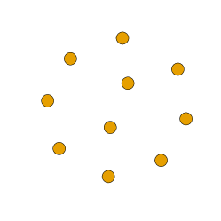
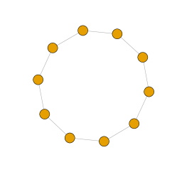
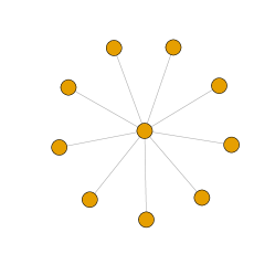
Figure 3: Three graphs with $d=10$ nodes: empty (left), ring (center) and star (right) graph.

9 Outlook on applications to Lévy processes

The theory of conditional independence and graphical models developed in this paper applies to general infinite measures $\Lambda$. We concentrated on discussing the implications of our results in the field of extreme value theory, since this field has been very active recently; see Sections 7.2 and 8.

Another important instance of a measure $\Lambda$ studied in this paper is the Lévy measure of an infinitely divisible random vector $X$ as introduced in Section 2.2. In this case, $\Lambda$ appears in the characteristic function of $X$ and it is not obvious which probabilistic interpretation a conditional independence statement $A\perp B\mid C\;[\Lambda]$ has. In the particular case where the Lévy measure $\Lambda$ concentrates on a finite number of rays this statement implies the classical conditional independence $X_{A}\perp\!\!\!\perp X_{B}\mid X_{C}$; see Section 7.3. For general Lévy measures this turns out to not be true.

Ongoing research shows that in this case a different and surprisingly intuitive probabilistic interpretation is available in terms of Lévy processes. A Lévy process $\{X(t):t\geq 0\}$ with values in $\mathbb{R}^{d}$ is a stochastic process with independent and stationary increments (e.g., Sato, 2013). Moreover, there is a one-to-one mapping that takes an infinitely divisible random vector $X$ with characteristic triplet $(0,0,\Lambda)$ to the associated Lévy process satisfying $X(1)\stackrel{{\scriptstyle d}}{{=}}X$; here we assume the drift and Gaussian component in Section 2.2 to be zero since they are well-understood. It turns out that our $\Lambda$ conditional independence characterizes conditional independence on the level of the sample paths of the Lévy process. Indeed, under the explosiveness assumption (E1) it can be shown that

$$\{X_{A}(t):t\geq 0\}\perp\!\!\!\perp\{X_{B}(t):t\geq 0\}\mid\{X_{C}(t):t\geq 0\}\quad\iff\quad A\perp B\mid C\;[\Lambda]$$

This result enables the definition of graphical models for Lévy processes with large potential for new theory, statistical methods and applications.

Appendix A Additional proofs for Sections 3 and 4: Conditional independence and additional characterization results

A.1 Consistency properties of the basic operations with measures

Lemma A.1.

Let $(A,B,C)$ be a partition of $V$ with $C\neq\emptyset$. Then

$$(\Lambda_{A\cup C})_{C}=\Lambda_{C},\qquad(\Lambda^{0}_{A\cup C})^{0}_{C}=\Lambda^{0}_{C},\qquad(\Lambda^{0}_{A\cup C})_{C}=(\Lambda_{B\cup C})^{0}_{C}.$$

Lemma A.2.

For a non-empty $D\subset V$ consider $Y\sim\mathbb{P}_{R_{D}\times\mathbb{R}^{V\setminus D}}$ with $R_{D}\in\mathcal{R}(\Lambda_{D})$. Then

1. $Y_{D}\sim\mathbb{P}_{R_{D}}$.

2. For any $R=R_{D}\times R_{V\setminus D}$ it holds that $\mathbb{P}_{R}$ is the conditional law of $Y$ given $Y_{V\setminus D}\in R_{V\setminus D}$.

Proof.

1. follows immediately from (7) and the definition of the marginal measure in (8).

2. is seen from

   $$\frac{\Lambda(\mathrm{d}y)}{\Lambda(R)}=\frac{\Lambda(\mathrm{d}y)}{\Lambda(R_{D}\times\mathbb{R}^{V\setminus D})}\frac{\Lambda(R_{D}\times\mathbb{R}^{V\setminus D})}{\Lambda(R)}=\frac{\mathbb{P}(Y\in\mathrm{d}y)}{\mathbb{P}(Y\in R)}$$

   for $y\in R$ and $Y_{D}\in R_{D}$ a.s. ∎

A.2 Restriction and extension

We start with a few fundamental results which follow directly from basic probability theory. We provide short arguments for completeness. Consider a partition $(A,B,C)$ of $V$. For two product-form sets $R,R^{\prime}\in\mathcal{R}(\Lambda)$ the corresponding random vectors as in (7) are denoted by $Y\sim\mathbb{P}_{R}$ and $Y^{\prime}\sim\mathbb{P}_{R^{\prime}}$ in the following.

Lemma A.3.

Let $C\neq\emptyset$. Assume that $R_{A\cup B}\supset R^{\prime}_{A\cup B}\supset E_{A\cup B}$, where the latter is some Borel set. Then

$$\mathbb{P}(Y^{\prime}_{A\cup B}\in E_{A\cup B}|Y^{\prime}_{C}=y_{C})=\frac{\mathbb{P}(Y_{A\cup B}\in E_{A\cup B}|Y_{C}=y_{C})}{\mathbb{P}(Y_{A\cup B}\in R^{\prime}_{A\cup B}|Y_{C}=y_{C})}$$

for $\mathbb{P}_{Y^{\prime}_{C}}$-almost all $y_{C}\in R_{C}\cap R^{\prime}_{C}$.

Proof.

Choose a Borel set $E_{C}\subset R_{C}\cap R^{\prime}_{C}$ and observe that

$$\mathbb{P}(Y^{\prime}_{A\cup B}\in E_{A\cup B},Y^{\prime}_{C}\in E_{C})=\mathbb{P}(Y_{A\cup B}\in E_{A\cup B},Y_{C}\in E_{C})\frac{\Lambda(R)}{\Lambda(R^{\prime})}.$$

The right hand side can be rewritten as

$$\int_{E_{C}}\frac{\mathbb{P}(Y_{A\cup B}\in E_{A\cup B}|Y_{C}=y_{C})}{\mathbb{P}(Y_{A\cup B}\in R^{\prime}_{A\cup B}|Y_{C}=y_{C})}\mathbb{P}(Y_{A\cup B}\in R^{\prime}_{A\cup B},Y_{C}\in\mathrm{d}y_{C})\frac{\Lambda(R)}{\Lambda(R^{\prime})},$$

where the denominator is non-zero for $\mathbb{P}_{Y^{\prime}_{C}}$-almost all $y_{C}\in E_{C}$. Note that the scaled measure corresponds to $\mathbb{P}(Y_{C}^{\prime}\in\mathrm{d}y)$ and thus we obtain

$$\mathbb{P}(Y^{\prime}_{A\cup B}\in E_{A\cup B},Y^{\prime}_{C}\in E_{C})=\int_{E_{C}}\frac{\mathbb{P}(Y_{A\cup B}\in E_{A\cup B}|Y_{C}=y_{C})}{\mathbb{P}(Y_{A\cup B}\in R^{\prime}_{A\cup B}|Y_{C}=y_{C})}\mathbb{P}(Y_{C}^{\prime}\in\mathrm{d}y_{C}),$$

and the result follows. ∎

Remark A.4.

1. If in addition $Y_{A}\perp\!\!\!\perp Y_{B}\mid Y_{C}$ in Lemma A.3, by setting $E_{A\cup B}=E_{A}\times R^{\prime}_{B}$, we can further conclude that for $\mathbb{P}_{Y^{\prime}_{C}}$-almost all $y_{C}\in R_{C}\cap R^{\prime}_{C}$

   $$\mathbb{P}(Y^{\prime}_{A}\in E_{A}|Y^{\prime}_{C}=y_{C})=\frac{\mathbb{P}(Y_{A}\in E_{A}|Y_{C}=y_{C})}{\mathbb{P}(Y_{A}\in R^{\prime}_{A}|Y_{C}=y_{C})},$$

   (and the analogous identity with reversed roles for $A$ and $B$).

2. We also note that, when $R^{\prime}_{A\cup B}=R_{A\cup B}$ in Lemma A.3, the two conditional probabilities $\mathbb{P}(Y^{\prime}_{A\cup B}\in E_{A\cup B}|Y^{\prime}_{C}=y_{C})$ and $\mathbb{P}(Y_{A\cup B}\in E_{A\cup B}|Y_{C}=y_{C})$ coincide for almost all $y_{C}\in R_{C}\cap R^{\prime}_{C}$ with respect to both probability measures $\mathbb{P}_{Y_{C}}$ and $\mathbb{P}_{Y^{\prime}_{C}}$.

3. For $C=\emptyset$ the analogous identity

   $$\mathbb{P}(Y^{\prime}_{A\cup B}\in E_{A\cup B})=\frac{\mathbb{P}(Y_{A\cup B}\in E_{A\cup B})}{\mathbb{P}(Y_{A\cup B}\in R^{\prime}_{A\cup B})}$$

   holds trivially.

Lemma A.5 (Restriction).

Assume that $R^{\prime}\subset R$. Then $Y_{A}\perp\!\!\!\perp Y_{B}\mid Y_{C}$ implies $Y^{\prime}_{A}\perp\!\!\!\perp Y^{\prime}_{B}\mid Y^{\prime}_{C}$. This result is also true for $C=\emptyset$ and the respective independence statements.

Proof.

Consider Borel subsets $E_{A}\subset R^{\prime}_{A}$ and $E_{B}\subset R^{\prime}_{B}$. According to Lemma A.3 and conditional independence $Y_{A}\perp\!\!\!\perp Y_{B}\mid Y_{C}$ we have

$$\mathbb{P}(Y^{\prime}_{A}\in E_{A},Y^{\prime}_{B}\in E_{B}|Y^{\prime}_{C}=y_{C})=\frac{\mathbb{P}(Y_{A}\in E_{A}|Y_{C}=y_{C})}{\mathbb{P}(Y_{A}\in R^{\prime}_{A}|Y_{C}=y_{C})}\,\frac{\mathbb{P}(Y_{B}\in E_{B}|Y_{C}=y_{C})}{\mathbb{P}(Y_{B}\in R^{\prime}_{B}|Y_{C}=y_{C})}$$

for $\mathbb{P}_{Y^{\prime}_{C}}$-almost all $y_{C}\in R^{\prime}_{C}$. By considering the same identity with $E_{B}=R^{\prime}_{B}$ and then $E_{A}=R^{\prime}_{A}$ and applying Lemma A.3 again, we find that the two ratios on the right-hand side are $\mathbb{P}(Y^{\prime}_{A}\in E_{A}|Y^{\prime}_{C}=y_{C})$ and $\mathbb{P}(Y^{\prime}_{B}\in E_{B}|Y^{\prime}_{C}=y_{C})$, respectively, and the first claim is proven. The case $C=\emptyset$ follows analogously from the trivial identity

$$\mathbb{P}(Y^{\prime}_{A}\in E_{A},Y^{\prime}_{B}\in E_{B})=\frac{\mathbb{P}(Y_{A}\in E_{A},Y_{B}\in E_{B})}{\mathbb{P}(Y_{A}\in R^{\prime}_{A},Y_{B}\in R^{\prime}_{B})}.\qed$$

Lemma A.6 (Extension via $C$).

Let $C\neq\emptyset$ and assume that $R^{\prime}_{A\cup B}=R_{A\cup B}$. Then $Y_{A}\perp\!\!\!\perp Y_{B}\mid Y_{C}$ and $Y^{\prime}_{A}\perp\!\!\!\perp Y^{\prime}_{B}\mid Y^{\prime}_{C}$ imply $Y^{\prime\prime}_{A}\perp\!\!\!\perp Y^{\prime\prime}_{B}\mid Y^{\prime\prime}_{C}$ with $Y^{\prime\prime}\sim\mathbb{P}_{R\cup R^{\prime}}$.

Proof.

Lemma A.3 shows that for any Borel subsets $E_{A}\subset R_{A},E_{B}\subset R_{B}$ we have

$$\mathbb{P}(Y^{\prime\prime}_{A}\in E_{A},Y^{\prime\prime}_{B}\in E_{B}|Y^{\prime\prime}_{C}=y_{C})=\mathbb{P}(Y_{A}\in E_{A},Y_{B}\in E_{B}|Y_{C}=y_{C})$$

$$=\mathbb{P}(Y_{A}\in E_{A}|Y_{C}=y_{C})\mathbb{P}(Y_{B}\in E_{B}|Y_{C}=y_{C})$$

$$=\mathbb{P}(Y^{\prime\prime}_{A}\in E_{A}|Y^{\prime\prime}_{C}=y_{C})\mathbb{P}(Y^{\prime\prime}_{B}\in E_{B}|Y^{\prime\prime}_{C}=y_{C})$$

for $\mathbb{P}_{Y^{\prime\prime}_{C}}$-almost all $y_{C}\in R_{C}$. Analogously, we get a factorization for $\mathbb{P}_{Y^{\prime\prime}_{C}}$-almost all $y_{C}\in R^{\prime}_{C}$ when considering $Y^{\prime}$ instead of $Y$. This shows the stated result. ∎

In Lemma A.6 we verify an extension result for conditional independence from two sets $R$ and $R^{\prime}$ with identical $A\cup B$ component to their union $R\cup R^{\prime}$. Naturally, the analogous extension result holds also for extending conditional independence from countably many product-form sets $R^{(n)}$ with $R^{(n)}_{A\cup B}=R_{A\cup B}$ for all $n$, resulting in the conditional independence statement on the union $\bigcup_{n}R^{(n)}$.

A.3 Main proofs for characterization results

We are now ready to prove our first characterization result.

Proof of Theorem 4.1.

By definition $A\perp B\mid C\,[\Lambda]$ implies $Y_{A}\perp\!\!\!\perp Y_{B}\mid Y_{C}$ with $Y\sim\mathbb{P}_{R_{v,{\varepsilon}}}$ for any $v\in V$ and ${\varepsilon}>0$ such that $\Lambda(R_{v,{\varepsilon}})>0$. Additionally, it implies $A\perp B\,[\Lambda^{0}_{A\cup B}]$, see Lemma 3.3. Thus $A\perp B\mid C\,[\Lambda]$ implies both (i) and (ii), also when $C=\emptyset$.

(i) In the opposite direction, we take any $R=\bigtimes R_{v}\in\mathcal{R}(\Lambda)$ and note that there exists $v\in V$ such that the closure of $R_{v}$ does not contain 0. Hence we may choose ${\varepsilon}>0$ such that $R\subset R_{v,{\varepsilon}}$. According to Lemma A.5 we have $Y_{A}\perp\!\!\!\perp Y_{B}\mid Y_{C}$ with $Y\sim\mathbb{P}_{R}$. Hence $A\perp B\mid C\,[\Lambda]$. The argument also applies when $C=\emptyset$.

(ii) It is sufficient to establish (i), and so we take any $v\in A\cup B$, ${\varepsilon}>0$ and consider the set $R_{v,{\varepsilon}}$. We partition this set according to $y_{C}\neq 0_{C}$ and $y_{C}=0_{C}$, letting $Y$ and $Y^{\prime}$ be the respective random vectors. Here we assume that both sets are charged by $\Lambda$, since otherwise the proof is only simpler. According to Lemma A.6 it is sufficient to show both $Y_{A}\perp\!\!\!\perp Y_{B}\mid Y_{C}$ and $Y^{\prime}_{A}\perp\!\!\!\perp Y^{\prime}_{B}\mid Y^{\prime}_{C}$.

The latter follows directly from $A\perp B\,[\Lambda^{0}_{A\cup B}]$, see also the proof of Lemma 3.3. The former follows from the countably-infinite version of Lemma A.6 by considering the sets $R^{(n,c)}=\{|y_{v}|\geq{\varepsilon},|y_{c}|\geq 1/n\}$ for all $c\in C$ and natural $n$. The respective conditional independence statements are implied by the assumption in (ii) together with the restriction Lemma A.5. ∎

As a side result the same argument that we used in proof of Theorem 4.1 (ii) above reveals that a single $v\in V$ can be taken when checking for conditional independence under the condition that $\Lambda(y\neq 0_{V},y_{v}=0)=0$. To be precise we formulate the following lemma.

Lemma A.7 (Single $v$ test).

Assume that a fixed $v\in V$ is such that $\Lambda(y\neq 0_{V},y_{v}=0)=0$. Then $Y_{A}\perp\!\!\!\perp Y_{B}\mid Y_{C}$ for all $Y\sim\mathbb{P}_{R_{v,{\varepsilon}}},{\varepsilon}>0$ implies $A\perp B\mid C\;[\Lambda]$. This result is also true for $C=\emptyset$ and the respective independence statements.

Next we prove uniqueness and representation of the kernel.

Proof of Lemma 4.3.

Let $R^{1}_{C}$ be some product form set bounded away from $0_{C}$ and define $R^{1}=\mathbb{R}^{A\cup B}\times R^{1}_{C}$. Suppose for a moment that $R_{C}\subset R^{1}_{C}$. Letting $Y\sim\mathbb{P}_{R^{1}}$ (the case of zero mass being trivial) we observe that

$$\Lambda(R)=\mathbb{P}(Y_{A\cup B}\in R_{A\cup B},Y_{C}\in R_{C})\Lambda(R^{1})=\int_{y_{C}\in R_{C}}\nu_{C}^{1}(y_{C},R_{A\cup B})\mathbb{P}(Y_{C}\in\mathrm{d}y_{C})\Lambda(R^{1}),$$

where $\nu_{C}^{1}(y_{C},\cdot)$ is a probability kernel corresponding to $Y$, see Kallenberg (2002, Thm. 6.3). Note that $\Lambda_{C}(\mathrm{d}y_{C})=\mathbb{P}(Y_{C}\in\mathrm{d}y_{C})\Lambda(R^{1}),y_{C}\in R_{C}$ giving the stated representation of $\Lambda(R)$. In general, we partition $\mathcal{E}^{C}$ into countably many product form sets $R^{i}_{C}$ and define $\nu_{C}(y_{C},\cdot)=\nu^{i}_{C}(y_{C},\cdot)$ for $y_{C}$ in the respective partition. The stated form of $\nu_{C}$ and $\Lambda_{C}$-uniqueness follow from Lemma A.3. ∎

Appendix B Further details for the generic construction of Section 5.4

Here we provide further details on the constructive example of a measure $\Lambda$ in $d=3$ dimensions with index set $V=\{1,2,3\}$ such that the conditional independence $\{1\}\perp\{3\}\mid\{2\}\;[\Lambda]$ holds. Table 1 contains the reformulation of the factorization of the modified density (18) in terms of original building blocks, that is, the densities $\kappa_{ij}$, their joint marginal density $m$ and the mixture probabilities $p_{ij}$ with $q_{ij}=1-p_{ij}$. Figure 4 illustrates them for faces up to dimension 2.

We note that if the starting density $\kappa$ is $-\alpha$-homogeneous for some $\alpha>2$, it is easily checked that its marginal density $m$ will be $-(\alpha-1)$-homogeneous and the resulting measure $\Lambda$ will be $-(\alpha-2)$-homogeneous; see Example 8.8.

Table 1: Modified densities of the trivariate example from Section 5.4; see also Figure 4. The resulting measure $\Lambda$ satisfies $\{1\}\perp\{3\}\mid\{2\}\;[\Lambda]$ and has identical one-dimensional marginals. It is globally Markov for the chain graph $1-2-3$ with zero mass on $\mathcal{Z}=\{y_{1}\neq 0,y_{2}=0,y_{3}\neq 0\}$; see Theorem 6.4.

Dimen-	Faces			Modified densities
sion	$y_{1}$	$y_{2}$	$y_{3}$	$\overline{\lambda}_{12}(y_{12})$	$\overline{\lambda}_{23}(y_{23})$	$\overline{\lambda}_{2}(y_{2})$	$\overline{\lambda}(y)=\lambda(y)$
	0	0	$\neq 0$	1	$q_{23}m(y_{3})$	1	$q_{23}m(y_{3})$
1	$\neq 0$	0	0	$q_{12}m(y_{1})$	1	1	$q_{12}m(y_{1})$
	0	$\neq 0$	0	$q_{12}m(y_{2})$	$q_{23}m(y_{2})$	$m(y_{2})$	$q_{12}q_{23}m(y_{2})$
	$\neq 0$	$\neq 0$	0	$p_{12}\kappa_{12}(y_{12})$	$q_{23}m(y_{2})$	$m(y_{2})$	$p_{12}q_{23}\kappa_{12}(y_{12})$
2	0	$\neq 0$	$\neq 0$	$q_{12}m(y_{2})$	$p_{23}\kappa_{23}(y_{23})$	$m(y_{2})$	$q_{12}p_{23}\kappa_{23}(y_{23})$
	$\neq 0$	0	$\neq 0$	$q_{12}m(y_{1})$	$q_{23}m(y_{3})$	1	$0$
3	$\neq 0$	$\neq 0$	$\neq 0$	$p_{12}\kappa_{12}(y_{12})$	$p_{23}\kappa_{23}(y_{23})$	$m(y_{2})$	$\frac{p_{12}p_{23}\kappa_{12}(y_{12})\kappa_{23}(y_{23})}{m(y_{2})}$

   

Figure 4: Illustration of the generic construction of a measure $\Lambda$ satisfying $\{1\}\perp\{3\}\mid\{2\}\;[\Lambda]$ from Section 5.4. Left: measure $\lambda_{ij}$, which serves as building block. Right: resulting densities $\lambda$ on the faces up to dimension 2; see Table 1.

Appendix C Additional proofs and examples for Section 6: Undirected graphical models

C.1 Auxiliary result for the Hammersley-Clifford-type theorem

Proposition C.1.

Assume that $\Lambda$ satisfies (E1) and that $V=D\cup C$ is the vertex set of a graph $\mathcal{G}$, where $C$ is a clique and $\widetilde{S}=D\cap C$ separates $D$ from $C$. Then $\Lambda$ satisfies the global Markov property with respect to $\mathcal{G}$ if and only if

$$D\setminus\widetilde{S}\perp C\setminus\widetilde{S}\mid\widetilde{S}\;[\Lambda]$$

and $\Lambda$ is globally Markov when restricted to $D$.

Proof of Proposition C.1.

The global Markov property for $\Lambda$ implies the other two properties. So we only need to establish the other direction, i.e. show the global Markov property for $\Lambda$. Consider disjoint set $A,B,S\subset V$ with $S$ separating $A$ from $B$. As outlined in Remark 6.2, it suffices to consider the partition situation, where $A\cup B\cup S=V$. Since $C$ is a clique, the sets $A$ and $B$ cannot both intersect $C$, otherwise they could not be separated by any $S$, so we may assume that $B\cap C=\emptyset$.

Let us first consider the case that $S\subset D$. Since $\Lambda$ satisfies (E1), we can employ the semi-graphoid property (L4). We do so with the four sets $(B,A\cap D,S,A\setminus D)$ as the sets $(A,B,C,D)$ from the original formulation of (L4). The first condition there reads as $B\perp(A\cap D)\mid S$, which is implied by the global Markov property for $D$. The second condition reads as $B\perp(A\setminus D)\mid S\cup(A\cap D)$, which follows from the other assumption, $(D\setminus{\widetilde{S}})\perp(A\setminus D)\mid{\widetilde{S}}$, by means of (L3). As a result we get $A\perp B\mid S$ as required.

If instead $E=S\cap(C\setminus\widetilde{S})\neq\emptyset$, set $A^{\prime}=A\cup E$ and $S^{\prime}=S\setminus E$. Then we can finish the proof by showing that $S^{\prime}$ still separates $A^{\prime}$ from $B$, but with $S^{\prime}\subset D$, so that we can employ the above argument again to obtain $A^{\prime}\perp B\mid S^{\prime}$, which subsequently implies $A\perp B\mid S$ by (L3). It remains to be seen that $S^{\prime}$ separates $A^{\prime}$ from $B$. The statement is trivially true if $\widetilde{S}=\emptyset$, since then no paths from $B$ to $E$ can exist. Else consider that if a path from $b\in B$ to $e\in E$ exists, it must pass through an element $v\in{\widetilde{S}}$ before reaching $C\setminus{\widetilde{S}}$ for the first time. Then either $v\in S$ or $v\in A$, in which case it must pass through another element from $S\cap D$, since $S$ separates $A$ from $B$. So it must intersect with $S^{\prime}$. Second, assume there exists a path from $b\in B$ to $a\in A$, whose intersection with $S$ is limited to $E$. Then there must be a first element $e\in E$ that is reached from $b\in B$ without intersecting $S^{\prime}$ and the same argument shows that this is impossible. ∎

C.2 Example for Remark 6.6

Consider the chain graph $1-2-3-4-5$ on the vertices $V=\{1,\ldots,5\}$ where the neighboring indices are connected. We construct a measure $\Lambda$ on $\mathcal{E}$ which is not(!) globally Markov with respect to this graph $\mathcal{G}$, even though

1. (E1) holds;

2. the density $\lambda$ satisfies the factorization

   $$\lambda(y)\lambda_{2}(y_{2})\lambda_{3}(y_{3})\lambda_{4}(y_{4})=\lambda_{12}(y_{12})\lambda_{23}(y_{23})\lambda_{34}(y_{34})\lambda_{45}(y_{45})$$

   for $\mu$-almost all $y$ such that $y_{2},y_{3},y_{4}\neq 0$;

3. $\Lambda(\mathcal{Z}(\mathcal{G}))=0$, that is, $\Lambda(y_{k}\neq 0,y_{l}=0,y_{m}\neq 0)=0$ whenever $k<l<m$.

As in Section 5.4 we consider the same dominating measure $\mu$ as in (16) (here for $d=5$) and use some $-3$-homogeneous bivariate densities $\kappa_{ij}$ on $(0,\infty)^{2}$ with marginal densities $y^{-2}$ as building blocks, now for $(i,j)\in\{(1,2),(2,3),(3,4),(4,5)\}$. In addition, we ensure that $\kappa_{12}$ and $\kappa_{23}$ are compatible with a $-4$-homogeneous trivariate density $\eta_{123}$ on $(0,\infty)^{3}$ as follows:

• $\eta_{12}=\kappa_{12},\eta_{23}=\kappa_{23}$ and, thus, respective univariate marginals have densities $y^{-2}$,

• $\eta_{123}(y_{123})\eta_{2}(y_{2})\neq\eta_{12}(y_{12})\eta_{23}(y_{23})$ on a subset of $(0,\infty)^{3}$ of positive Lebesgue measure.

The second condition is equivalent to saying that the measure corresponding to $\eta_{123}$ does not induce the conditional independence of $1$ and $3$ given $2$, see Theorem 4.6. Such a construction is always possible, e.g. one can start from $\eta_{123}$ with the respective univariate marginals and then work with $\kappa_{12}$ and $\kappa_{23}$ that arise from $\eta_{123}$. From there, we define

$$\lambda(y)=\begin{cases}\kappa_{12}(y_{12})\kappa_{23}(y_{23})\kappa_{34}(y_{34})\kappa_{45}(y_{45})y_{2}^{2}y_{3}^{2}y_{4}^{2},&y_{1},y_{2},y_{3},y_{4},y_{5}>0,\\ \eta_{123}(y_{123}),&y_{1},y_{2},y_{3}>0,y_{4}=y_{5}=0,\end{cases}$$

and let it be 0 otherwise. By construction, the measure $\Lambda$ satisfies the conditions (i) and (iii). Furthermore, the bivariate marginals on $(0,\infty)^{2}$ are given by

$$\lambda_{12}=\kappa_{12}+\eta_{12}=2\kappa_{12},\quad\lambda_{23}=\kappa_{23}+\eta_{23}=2\kappa_{23},\quad\lambda_{34}=\kappa_{34},\quad\lambda_{45}=\kappa_{45},$$

and the univariate ones by $\lambda_{2}(y_{2})=2y_{2}^{-2},\lambda_{3}(y_{3})=2y_{3}^{-2},\lambda_{4}(y_{4})=y_{4}^{-2}$. This readily yields the factorization in (ii). Finally, we note that $\Lambda$ is not globally Markov for the chain graph since $\{1\}\perp\{3,4,5\}\mid\{2\}\;[\Lambda]$ is not true, because

$$\lambda(y)\lambda_{2}(y_{2})=\eta_{123}(y_{123})2y_{2}^{-2}\neq 2\eta_{12}(y_{12})\eta_{23}(y_{23})=\lambda_{12}(y_{12})\lambda_{2345}(y_{2345})$$

on the subset $\{y:y_{1},y_{2},y_{3}>0,y_{4}=y_{5}=0\}$, which has positive $\mu$-mass. Hence, according to Theorem 4.6 the condition $\{1\}\perp\{3,4,5\}\mid\{2\}\;[\Lambda]$ is violated.

Had we checked instead the factorization condition from Theorem 6.4 in terms of $\overline{\lambda}$ on this set, we would have picked up the violation of the global Markov property. The left-hand side of (20) reads $\eta_{123}(y_{123})2y_{2}^{-2}2y_{3}^{-2}$ in this case, and the right-hand side is $2\eta_{12}(y_{12})2\eta_{23}(y_{23})y_{3}^{-2}$. They cannot be equal due to our choice of $\eta_{123}$.

Appendix D Additional proofs for Section 8

D.1 Derivation of extremal correlation $\chi_{ij}$ in Example 8.8

Proof.

For $i\nleftrightarrow j$, since $\Lambda$ is a graphical model on the forest $\mathcal{G}$, the global Markov property implies that $i\perp j\;[\Lambda]$. By Proposition 5.1 we therefore have that $\Lambda(y_{i}\neq 0,y_{j}\neq 0)=0$, which yields $\chi_{ij}=0$ according to (31).

For $i\leftrightarrow j$ we note that by homogeneity we have $\chi_{ij}=\Lambda(y_{i}>1,y_{j}>1)/\Lambda(1)$ and $\Lambda(1)=1$. Because of the density factorization (34) we can first integrate out all components $k\notin\mathrm{path}_{ij}$ to get

$$\Lambda(y_{i}>1,y_{j}>1)=\int_{1}^{\infty}\int_{1}^{\infty}\int_{(0,\infty)^{|V(ij)|}}\frac{\prod_{(s,t)\in\mathrm{path}_{ij}}\overline{\lambda}_{st}(y_{s},y_{t})}{\prod_{s\in V(ij)}\overline{\lambda}_{s}(y_{s})}\mathrm{d}y_{i}\mathrm{d}y_{j}\mathrm{d}y_{V(ij)},$$

where $V(ij)$ denotes all nodes on the path from $i$ to $j$, excluding $i$ and $j$. Thus,

$$\chi_{ij}=\int_{1}^{\infty}\int_{1}^{\infty}\int_{(0,\infty)^{|V(ij)|}}\frac{\prod_{(s,t)\in\mathrm{path}_{ij}}p_{st}\kappa_{st}(y_{s},y_{t})}{\prod_{s\in V(ij)}y_{s}^{-2}}\mathrm{d}y_{i}\mathrm{d}y_{j}\mathrm{d}y_{V(ij)}=\chi_{ij}^{\text{HR}}\prod_{(s,t)\in\mathrm{path}_{ij}}p_{st}$$

where $\chi_{ij}^{\text{HR}}=2-2\Phi(\sqrt{\Gamma_{ij}}/2)$ with $\Gamma_{ij}=\sum_{(s,t)\in\mathrm{path}_{ij}}\Gamma_{st}$ is the extremal correlation of the corresponding tree model on the connected component that contains $i$ and $j$ (Engelke and Volgushev, 2020, Proposition 4). This result is true since the domain of the above integral is contained in the set $\{y_{i}>0,y_{j}>0,y_{V(ij)}>0\}$, on which the density coincides with the usual Hüsler–Reiss tree model.

∎

D.2 Proof of Lemma 8.9: Max-infinitely divisibility and asymptotic equivalence of the joint survival functions

Proof.

Denoting $\Lambda_{ij}(u,u)=\Lambda_{ij}(y_{i}>u\text{ or }y_{j}>u)$, we can rewrite

$$\mathbb{P}(Z_{i}>u,Z_{j}>u) =1-2e^{-\Lambda(u)}+e^{-\Lambda_{ij}(u,u)}.$$ (40)

Using $\Lambda_{ij}(u,u)\leq 2\Lambda(u)$ for all $u>0$ gives

$$\mathbb{P}(Z_{i}>u,Z_{j}>u)\geq 1-2e^{-\Lambda(u)}+e^{-2\Lambda(u)}=(1-e^{-\Lambda(u)})^{2}=\mathbb{P}(Z_{i}>u)^{2}.$$

Together with (30) we obtain $\eta_{ij}\geq 1/2$.

Now suppose that $\eta_{ij}>1/2$ and recall the bounds $1-x\leq e^{-x}\leq 1-x+x^{2}/2$ for all $x>0$. Applied to (40) we obtain upper and lower bounds for $\mathbb{P}(Z_{i}>u,Z_{j}>u)$ as follows:

$$2\Lambda(u)-\Lambda_{ij}(u,u)-\Lambda(u)^{2}\leq\mathbb{P}(Z_{i}>u,Z_{j}>u) \leq 2\Lambda(u)-\Lambda_{ij}(u,u)+\Lambda_{ij}(u,u)^{2}/2$$

$$\leq 2\Lambda(u)-\Lambda_{ij}(u,u)+2\Lambda(u)^{2}.$$

Since $\Lambda(y_{i}>u,y_{j}>u)=2\Lambda(u)-\Lambda_{ij}(u,u)$, we may rewrite these bounds as

$$\mathbb{P}(Z_{i}>u,Z_{j}>u)-2\Lambda(u)^{2}\leq\Lambda(y_{i}>u,y_{j}>u)\leq\mathbb{P}(Z_{i}>u,Z_{j}>u)+\Lambda(u)^{2}.$$

Hence, we obtain the assertion from

$$\lim_{u\to\infty}\frac{\Lambda(u)^{2}}{\mathbb{P}(Z_{i}>u,Z_{j}>u)}=0,$$

which holds since $\eta_{ij}>1/2$. ∎

D.3 Proof of Proposition 8.11: An asymptotically independent example based on Gaussian distributions

We provide an explicit construction of an exponent measure $\Lambda$ in dimension 3, which satisfies the conditional independence $\{1\}\perp\{3\}\mid\{2\}\;[\Lambda]$, but exhibits otherwise asymptotic independence. It is based on two bivariate Gaussian distributions and we will need some auxiliary results in order to derive and quantify the asymptotic independence in the sense of Ledford and Tawn (1996).

Let $\Phi$ and $\varphi$ be the cdf and pdf of the univariate standard Gaussian distribution, and let $\overline{\Phi}(x)=1-\Phi(x)=\Phi(-x)$ be the corresponding survival function. It is well-known (DLMF, , Eq. 7.8.2) that

$$\frac{2}{x+\sqrt{x^{2}+4}}<\frac{\overline{\Phi}(x)}{\varphi(x)}<\frac{2}{x+\sqrt{x^{2}+8/\pi}}<\frac{1}{x},\qquad x>0.$$ (41)

Using (41), one may easily derive the following result by showing positivity of the respective derivatives (e.g., Resnick, 2008, Lemma 5.4).

Lemma D.1.

The functions $\Phi/\varphi$ and $\varphi/\overline{\Phi}$ are strictly monotonously increasing on its entire domain $\mathbb{R}=(-\infty,\infty)$ from $0$ to $\infty$.

As any univariate distribution, $\Phi$ is max-infinitely divisible. Its exponent measure $\Lambda_{1}$ is supported on $\mathbb{R}=(-\infty,\infty)$ with survival function

$$\Lambda(u)=\Lambda_{1}((u,\infty))=-\log\Phi(u),\qquad u\in\mathbb{R}$$

and density

$$\lambda_{1}(u)=\frac{\partial}{\partial u}\log\Phi(u)=\frac{\varphi(u)}{\Phi(u)},\qquad u\in\mathbb{R}.$$

It is immediate that the survival functions of $\Lambda_{1}$ and $\Phi$ are asymptotically equivalent in the sense that

$$\lim_{u\to\infty}\frac{\Lambda(u)}{\overline{\Phi}(u)}=1.$$ (42)

Let $\Phi_{\rho}$ and $\varphi_{\rho}$ be the cdf and pdf of the bivariate normal distribution with standard Gaussian margins and correlation $\rho$. Some useful identities, which we will use in several arguments below, are

$$\frac{\partial}{\partial x_{1}}\Phi_{\rho}(x_{1},x_{2}) =\Phi\bigg{(}\frac{x_{2}-\rho x_{1}}{\sqrt{1-\rho^{2}}}\bigg{)}\varphi(x_{1}),\qquad\frac{\partial}{\partial x_{2}}\Phi_{\rho}(x_{1},x_{2})=\Phi\bigg{(}\frac{x_{1}-\rho x_{2}}{\sqrt{1-\rho^{2}}}\bigg{)}\varphi(x_{2}),$$

$$\sqrt{1-\rho^{2}}\,\varphi_{\rho}(x_{1},x_{2}) =\varphi\bigg{(}\frac{x_{2}-\rho x_{1}}{\sqrt{1-\rho^{2}}}\bigg{)}\varphi(x_{1})=\varphi\bigg{(}\frac{x_{1}-\rho x_{2}}{\sqrt{1-\rho^{2}}}\bigg{)}\varphi(x_{2}).$$

Lemma D.2.

For $x_{1},x_{2}\in\mathbb{R}$ and $\rho\in(0,1)$

$$\max\bigg{[}\Phi(x_{1})\Phi\bigg{(}\frac{x_{2}-\rho x_{1}}{\sqrt{1-\rho^{2}}}\bigg{)},\Phi(x_{2})\Phi\bigg{(}\frac{x_{1}-\rho x_{2}}{\sqrt{1-\rho^{2}}}\bigg{)}\bigg{]}\leq\Phi_{\rho}(x_{1},x_{2})$$

and

$$\Phi_{\rho}(x_{1},x_{2})\leq\min\bigg{[}\Phi(x_{1})\Phi\bigg{(}\frac{x_{2}-\rho x_{1}}{\sqrt{1-\rho^{2}}}\bigg{)}+\Phi(x_{2}),\Phi(x_{2})\Phi\bigg{(}\frac{x_{1}-\rho x_{2}}{\sqrt{1-\rho^{2}}}\bigg{)}+\Phi(x_{1})\bigg{]}.$$

Proof.

Consider

$$H_{\rho}(x_{1},x_{2})=\Phi_{\rho}(x_{1},x_{2})-\Phi(x_{1})\Phi\bigg{(}\frac{x_{2}-\rho x_{1}}{\sqrt{1-\rho^{2}}}\bigg{)}.$$

It is easily seen that $H_{\rho}(x_{1},x_{2})$ converges to $0$ for $x_{1}\to-\infty$ and to $\Phi(x_{2})$ for $x_{1}\to\infty$. Moreover,

$$\frac{\partial}{\partial x_{1}}H_{\rho}(x_{1},x_{2}) =\frac{\rho}{\sqrt{1-\rho^{2}}}\varphi\bigg{(}\frac{x_{2}-\rho x_{1}}{\sqrt{1-\rho^{2}}}\bigg{)}\Phi(x_{1})$$

is positive. Hence $H_{\rho}(x_{1},x_{2})$ is strictly increasing in $x_{1}$ and ranges between $0$ and $\Phi(x_{2})$. Exchanging the roles of $x_{1}$ and $x_{2}$ establishes the assertion. ∎

We shall abbreviate the corresponding joint survival function of $\Phi_{\rho}$ by

$$S_{\rho}(x_{1},x_{2})=\mathbb{P}(X_{1}>x_{1},X_{2}>x_{2}),$$

where $(X_{1},X_{2})$ is distributed according to $\Phi_{\rho}$. By an argument of Balkema (Resnick, 2008, Section 5.2), the bivariate Gaussian distribution $\Phi_{\rho}$ is max-infinitely divisible if and only if $\rho\geq 0$. If $\rho\in(0,1)$, the associated exponent measure $\Lambda^{(\rho)}$ has a positive continuous density on $\mathbb{R}^{2}=(-\infty,\infty)^{2}$ as given by

$$\lambda^{(\rho)}(x_{1},x_{2})=\frac{\partial}{\partial x_{1}}\frac{\partial}{\partial x_{2}}\log\Phi_{\rho}(x_{1},x_{2})=\frac{\varphi_{\rho}(x_{1},x_{2})}{\Phi_{\rho}(x_{1},x_{2})}\kappa^{(\rho)}(x_{1},x_{2}),$$

where

$$\kappa^{(\rho)}(x_{1},x_{2})=1-\frac{\varphi(x_{1})\varphi(x_{2})\Phi\Big{(}\frac{x_{1}-\rho x_{2}}{\sqrt{1-\rho^{2}}}\Big{)}\Phi\Big{(}\frac{x_{2}-\rho x_{1}}{\sqrt{1-\rho^{2}}}\Big{)}}{\varphi_{\rho}(x_{1},x_{2})\Phi_{\rho}(x_{1},x_{2})}.$$

Evidently, $\kappa^{(\rho)}\leq 1$. By the max-infinitely divisibility property of $\Phi_{\rho}$, it is clear that $\kappa^{(\rho)}\geq 0$. It can be further uniformly bounded as follows.

Lemma D.3.

Let $\rho\in(0,1)$. For $\max(x_{1},x_{2})\geq 0$ we have

$$0<1-\sqrt{1-\rho^{2}}\leq\kappa^{(\rho)}(x_{1},x_{2}).$$

Moreover, there exists a constant $C_{\rho}>0$ such that for $u>0$

$$1-C_{\rho}u^{-1}\leq\inf_{x_{1},x_{2}\geq u}\kappa^{(\rho)}(x_{1},x_{2}).$$

Proof.

First note that for all $x_{1},x_{2}\in\mathbb{R}$

$$\frac{\varphi(x_{1})\varphi(x_{2})}{\varphi_{\rho}(x_{1},x_{2})}=\frac{\sqrt{1-\rho^{2}}\varphi(x_{1})}{\varphi\Big{(}\frac{x_{1}-\rho x_{2}}{\sqrt{1-\rho^{2}}}\Big{)}}$$

and by Lemma D.2

$$\frac{\Phi\Big{(}\frac{x_{1}-\rho x_{2}}{\sqrt{1-\rho^{2}}}\Big{)}\Phi\Big{(}\frac{x_{2}-\rho x_{1}}{\sqrt{1-\rho^{2}}}\Big{)}}{\Phi_{\rho}(x_{1},x_{2})}\leq\frac{1}{\Phi(x_{1})}\Phi\bigg{(}\frac{x_{1}-\rho x_{2}}{\sqrt{1-\rho^{2}}}\bigg{)},$$

which gives (by repeating this argument with reversed roles for $x_{1}$ and $x_{2}$)

$$1-\kappa^{(\rho)}(x_{1},x_{2}) \leq\sqrt{1-\rho^{2}}\,\min\bigg{[}\frac{\varphi(x_{1})}{\Phi(x_{1})}\frac{\Phi\Big{(}\frac{x_{1}-\rho x_{2}}{\sqrt{1-\rho^{2}}}\Big{)}}{\varphi\Big{(}\frac{x_{1}-\rho x_{2}}{\sqrt{1-\rho^{2}}}\Big{)}},\frac{\varphi(x_{2})}{\Phi(x_{2})}\frac{\Phi\Big{(}\frac{x_{2}-\rho x_{1}}{\sqrt{1-\rho^{2}}}\Big{)}}{\varphi\Big{(}\frac{x_{2}-\rho x_{1}}{\sqrt{1-\rho^{2}}}\Big{)}}\bigg{]}$$ (43)

$$=\sqrt{1-\rho^{2}}\,\min\bigg{[}{H\bigg{(}\frac{x_{1}-\rho x_{2}}{\sqrt{1-\rho^{2}}}\bigg{)}}/{H(x_{1})},{H\bigg{(}\frac{x_{2}-\rho x_{1}}{\sqrt{1-\rho^{2}}}\bigg{)}}/{H(x_{2})}\bigg{]},$$

where $H=\Phi/\varphi$. It suffices to show that the last minimum is not larger than 1 for $x_{1}\geq 0$. We will distinguish three cases.
Case 1: $0\leq x_{1}\leq x_{2}$. First note that $\rho\in(0,1)$ implies $q=(1-\sqrt{1-\rho^{2}})/\rho\in(0,1)$ and hence $qx_{1}\leq x_{2}$, which implies

$$\frac{x_{1}-\rho x_{2}}{\sqrt{1-\rho^{2}}}\leq x_{1}.$$

By the monotonicity of $H$ (see Lemma D.1) the assertion follows.
Case 2a: $0\leq x_{2}\leq x_{1}$. We can repeat the argument of Case 1 with reversed roles for $x_{1}$ and $x_{2}$.
Case 2b: $x_{2}\leq x_{1}$, $x_{1}\geq 0$, $x_{2}=-y<0$. In this situation, we can rewrite

$$H\bigg{(}\frac{x_{2}-\rho x_{1}}{\sqrt{1-\rho^{2}}}\bigg{)}/H(x_{2})=\widetilde{H}(y)/\widetilde{H}\bigg{(}\frac{y+\rho x_{1}}{\sqrt{1-\rho^{2}}}\bigg{)},$$

where $\widetilde{H}(x)=1/H(-x)=\varphi(x)/\overline{\Phi}(x)$ is also monotonously increasing (see Lemma D.1). Since $y\leq(y+\rho x_{1})/\sqrt{1-\rho^{2}}$, we can bound the right-hand side by 1 and the assertion follows.

For the second assertion, without loss of generality, assume $x_{1}\geq x_{2}\geq u>0$ and recall from (43) that

$$\frac{\Phi(0)}{\sqrt{1-\rho^{2}}}\big{(}1-\kappa^{(\rho)}(x_{1},x_{2})\big{)} \leq\frac{\Phi(0)}{\Phi(x_{2})}\varphi(x_{2})\frac{\Phi\Big{(}\frac{x_{2}-\rho x_{1}}{\sqrt{1-\rho^{2}}}\Big{)}}{\varphi\Big{(}\frac{x_{2}-\rho x_{1}}{\sqrt{1-\rho^{2}}}\Big{)}}\leq{\varphi(x_{2})}\frac{\Phi\Big{(}\frac{x_{2}-\rho x_{1}}{\sqrt{1-\rho^{2}}}\Big{)}}{\varphi\Big{(}\frac{x_{2}-\rho x_{1}}{\sqrt{1-\rho^{2}}}\Big{)}}.$$ (44)

We distinguish three cases according to the value of $q=x_{2}/x_{1}\in(0,1]$:
Case 1: $q\in(0,\rho/2]$. Then $-(x_{2}-\rho x_{1})=(\rho-q)x_{1}>\rho/2\cdot u$ and the right-hand side of (44) is bounded by ${2\varphi(0)\sqrt{1-\rho^{2}}}/{\rho}\cdot u^{-1}$ according to (41).
Case 2: $q\in(\rho/2,\rho)$. Then $x_{2}-\rho x_{1}=-(\rho-q)x_{1}<0$ and $x_{2}=qx_{1}>\rho/2\cdot u$. With Lemma D.1, we obtain that the right-hand side of (44) is bounded by $\Phi(0)/\varphi(0)\varphi(\rho/2\cdot u)$.
Case 3: $q\in[\rho,1]$. In this situation $x_{2}-\rho x_{1}=(q-\rho)x_{1}$ is positive. We also recall $\rho/(1-\sqrt{1-\rho^{2}})>1\geq q$, which implies

$$q>\frac{q-\rho}{\sqrt{1-\rho^{2}}}>0.$$

Hence, we can bound the right-hand side of (44) by $\Phi(0)$ multiplied with

$$\sup_{q\in[\rho,1]}\frac{\varphi(qx_{1})}{\varphi\Big{(}\frac{(q-\rho)x_{1}}{\sqrt{1-\rho^{2}}}\Big{)}}\leq\exp\bigg{\{}-\frac{1}{2}\inf_{q\in[\rho,1]}\Big{[}q^{2}-\Big{(}\frac{q-\rho}{\sqrt{1-\rho^{2}}}\Big{)}^{2}\Big{]}x_{1}^{2}\bigg{\}}\leq\exp(-\rho^{2}u^{2}/2).$$

Taken together, all three cases establish the assertion. ∎

Lemma D.4.

Let $\rho\in(0,1)$. The joint survival functions $\Lambda^{(\rho)}$ and $S_{\rho}$ are asymptotically equivalent in the sense that

$$\lim_{u\to\infty}\frac{\Lambda^{(\rho)}((u,\infty)^{2})}{S_{\rho}(u,u)}=1.$$

Proof.

By definition, we have

$$\Lambda^{(\rho)}((u,\infty)^{2})=2(-\log\Phi(u))-(-\log\Phi_{\rho}(u,u))$$

and

$$S_{\rho}(u,u)=2(1-\Phi(u))-(1-\Phi_{\rho}(u,u)).$$

Applying L’Hopital’s rule yields

$$\lim_{u\to\infty}\frac{\Lambda^{(\rho)}((u,\infty)^{2})}{S_{\rho}(u,u)} =\lim_{u\to\infty}\frac{2{\varphi(u)}/{\Phi(u)}-{2\varphi(u)\Phi(su)}/{\Phi_{\rho}(u,u)}}{2\varphi(u)-2\varphi(u)\Phi(su)}$$

$$=\lim_{u\to\infty}\frac{1}{\Phi_{\rho}(u,u)\Phi(u)}\cdot\lim_{u\to\infty}\frac{\Phi_{\rho}(u,u)-\Phi(su)\Phi(u)}{1-\Phi(su)},$$

where $s=(1-\rho)/\sqrt{1-\rho^{2}}=\sqrt{(1+\rho)/(1-\rho)}\in(0,1)$. As the involved cdfs converge to 1, it remains to be seen that the second limit equals 1. Indeed,

$$\lim_{u\to\infty}\frac{\Phi_{\rho}(u,u)-\Phi(su)\Phi(u)}{1-\Phi(su)} =\lim_{u\to\infty}\frac{2\varphi(u)\Phi(su)-s\varphi(su)\Phi(u)-\varphi(u)\Phi(su)}{-s\varphi(su)}$$

$$=\lim_{u\to\infty}\Phi(u)-\lim_{u\to\infty}\frac{\varphi(u)}{\varphi(su)}\cdot\lim_{u\to\infty}\frac{\Phi(su)}{s}=1-0/s=1,$$

hence the assertion. ∎

In what follows we will need a few simple facts about regularly varying functions. An eventually positive measurable function that is defined in a neighborhood of $\infty\in\mathbb{R}$, is regularly varying with index $\alpha\in\mathbb{R}$ (we write $f\in\mathrm{RV}_{\alpha}$) if $f(st)/f(t)\to s^{-\alpha}$ for $t\to\infty$. The case $\alpha=0$ is a special case, $f$ is then called slowly varying. Trivially, $\log(t)$, $1/\log(t)$ or any measurable function that converges to a positive constant is slowly varying. Some well-known closure properties are as follows (e.g., de Haan and Ferreira, 2006, Appendix B).

Lemma D.5.

If $f_{1}\in\mathrm{RV}_{\alpha_{1}}$, $f_{2}\in\mathrm{RV}_{\alpha_{2}}$, then $f_{1}+f_{2}\in\mathrm{RV}_{\max(\alpha_{1},\alpha_{2})}$ and $f_{1}f_{2}\in\mathrm{RV}_{\alpha_{1}+\alpha_{2}}$. If in addition $f_{2}(t)\to\infty$ for $t\to\infty$, then the composition satisfies $f_{1}\circ f_{2}\in\mathrm{RV}_{\alpha_{1}\alpha_{2}}$.

We will need to be aware of the following consequence.

Lemma D.6.

Let $a(u)=\overline{\Phi}(u)^{-1}$ and $b(u)=\Lambda(u)^{-1}$. Then $f\circ a^{-1}$ is slowly varying if and only if $f\circ b^{-1}$ is slowly varying.

Proof.

Since $a\circ b^{-1}(t)/t\to 1$ for $t\to\infty$, we have $a\circ b^{-1}\in\mathrm{RV}_{1}$ and $a\circ b^{-1}(t)\to\infty$ for $t\to\infty$. So, if $f\circ a^{-1}\in\mathrm{RV}_{0}$, so is $f\circ b^{-1}=(f\circ a^{-1})\circ(a\circ b^{-1})$ by Lemma D.5. The converse follows analogously. ∎

Coming back to the Gaussian joint survival functions, it is well-known that for $\eta_{\rho}=(1+\rho)/2$

$$S_{\rho}(u,u)=\ell_{\rho}(\overline{\Phi}(u)^{-1})\overline{\Phi}(u)^{1/\eta_{\rho}}$$ (45)

for a slowly varying function $\ell_{\rho}$ as $u\to\infty$ (Ledford and Tawn, 1996). In other words, the distribution $\Phi_{\rho}$ exhibits asymptotic independence; see Section 8.2.

Due to the asymptotic equivalences from (42) and Lemma D.4 and, in addition, Lemma D.6, this relation carries over to the asymptotically equivalent counterparts, that is,

$$\Lambda^{(\rho)}((u,\infty)^{2})=\widetilde{\ell}_{\rho}(\Lambda(u)^{-1})\Lambda(u)^{1/\eta_{\rho}}$$ (46)

for a slowly varying function $\widetilde{\ell}_{\rho}$. In particular,

$$\chi_{\rho}=\lim_{u\to\infty}\frac{\Lambda^{(\rho)}((u,\infty)^{2})}{\Lambda(u)}=\lim_{u\to\infty}\frac{S_{\rho}(u,u)}{\overline{\Phi}(u)}=0.$$ (47)

Moreover, moving from a multivariate Gaussian distribution $F$ on $\mathbb{R}^{d}=(-\infty,\infty)^{d}$ to a log-Gaussian distribution $F\circ\log$ on $(0,\infty)^{d}$ only requires a (componentwise) log-transformation, and the same applies to the corresponding exponent measures; that is, $\Lambda_{1}\circ\log$ is the exponent measure of $\Phi\circ\log$ and $\Lambda^{(\rho)}\circ\log$ is the exponent measure of $\Phi_{\rho}\circ\log$. Hence, the relations (42), (46) and (47) all carry over to the log-Gaussian variant on $(0,\infty)$ and $(0,\infty)^{2}$ by realizing that one can replace $u$ by $\log(u)$ in all situations. For notational convenience, we shall remain on the Gaussian scale in what follows, even though the construction could also be carried out on the log-Gaussian scale. In essence, this corresponds to replacing $0$ by $-\infty$ as the absorbing state, whilst the framework of conditional independence carries over with only minor modifications; see also Remark 3.2.

Now let $a,b\in(0,1)$ and consider a trivariate exponent measure $\Lambda$ on $\mathbb{R}^{3}$ with density

$$\lambda(x)=\frac{\lambda^{(a)}(x_{1},x_{2})\lambda^{(b)}(x_{2},x_{3})}{\lambda_{1}(x_{2})},\qquad x\in\mathbb{R}^{3},$$

similarly to the example of Section 5.4 with $p_{12}=p_{23}=1$. This ensures that the marginal measures of $\Lambda$ are given by

$$\Lambda_{12}=\Lambda^{(a)}\qquad\text{and}\qquad\Lambda_{23}=\Lambda^{(b)},$$

whilst the transformation of $\Lambda$ to log-Gaussian scale satisfies the conditional independence relation

$$\{1\}\perp\{3\}\mid\{2\}\;[\Lambda\circ\log].$$

From the above considerations, we know that

$$\chi_{12}=\chi_{a}=0,\quad\eta_{12}=\frac{1+a}{2},\quad\chi_{23}=\chi_{b}=0\quad\text{and}\quad\eta_{23}=\eta_{b}=\frac{1+b}{2}.$$ (48)

In order to derive the corresponding values for $\chi_{13}$ and $\eta_{13}$, we need to investigate the asymptotic behavior of

$$\Lambda_{13}((u,\infty)^{2})=\int_{u}^{\infty}\int_{-\infty}^{\infty}\int_{u}^{\infty}\lambda(x)\mathrm{d}x_{1}\mathrm{d}x_{2}\mathrm{d}x_{3}$$ (49)

in relation to $\Lambda(u)$ as $u\uparrow\infty$.

Note that $\Lambda_{13}$ is different from the bivariate exponent measure $\Lambda^{(ab)}$, which would have arisen as marginal exponent measure of $(X_{1},X_{3})$ of a trivariate Gaussian distribution $(X_{1},X_{2},X_{3})$ with $(X_{1},X_{2})\sim\Phi_{a}$, $(X_{2},X_{3})\sim\Phi_{b}$ and $X_{1}\perp\!\!\!\perp X_{3}\mid X_{2}$ (it is easily seen that the inverse $Q$ of the correlation matrix $\Sigma$ with entries $\rho_{12}=a$, $\rho_{23}=b$, $\rho_{13}=ab$ satisfies $Q_{13}=0$; an easy way to verify that $\Lambda_{13}\neq\Lambda^{(ab)}$ is by considering the trivariate zero mean Gaussian distribution with covariance matrix $\Sigma$ and by observing that the value at $0\in\mathbb{R}^{3}$ of a hypothetical density of its exponent measure, if it existed, deviates from $\lambda(0)$).

However, we bear in mind that

$$\varphi_{ab}(x_{1},x_{3})=\int_{-\infty}^{\infty}\widetilde{\varphi}(x)\mathrm{d}x_{2}\qquad\text{with}\qquad\widetilde{\varphi}(x)=\frac{\varphi_{a}(x_{1},x_{2})\varphi_{b}(x_{2},x_{3})}{\varphi(x_{2})},$$

and that

$$\lambda^{(ab)}(x_{1},x_{3})=\frac{\varphi_{ab}(x_{1},x_{3})}{\Phi_{ab}(x_{1},x_{3})}\kappa^{(ab)}(x_{1},x_{3})=\int_{-\infty}^{\infty}\widetilde{\varphi}(x)\,\mathrm{d}x_{2}\,\frac{\kappa^{(ab)}(x_{1},x_{3})}{\Phi_{ab}(x_{1},x_{3})}.$$

The density of $\Lambda_{13}$ is instead given by

$$\lambda_{13}(x_{1},x_{3}) =\int_{-\infty}^{\infty}\lambda(x)\mathrm{d}x_{2}$$

$$=\int_{-\infty}^{\infty}\frac{\lambda^{(a)}(x_{1},x_{2})\lambda^{(b)}(x_{2},x_{3})}{\lambda_{1}(x_{2})}\mathrm{d}x_{2}$$

$$=\int_{-\infty}^{\infty}\widetilde{\varphi}(x)\,\frac{\Phi(x_{2})}{\Phi_{a}(x_{1},x_{2})\Phi_{b}(x_{2},x_{3})}\,{\kappa^{(a)}(x_{1},x_{2})\kappa^{(b)}(x_{2},x_{3})}\mathrm{d}x_{2}.$$

Although, $\Lambda_{13}\neq\Lambda^{(ab)}$, these measures do not deviate too significantly from each other in their joint upper tails. In order to see this, all we need to do is to control the behavior of the additional multiplicative terms in the integrand above that appear in addition to the term $\widetilde{\varphi}(x)$.

Lemma D.7.

There exist $C>0$ such that for $x_{1},x_{3}\geq 0$

$$\frac{\Phi(x_{2})}{\Phi_{a}(x_{1},x_{2})\Phi_{b}(x_{2},x_{3})}\leq C\frac{1}{\Phi(x_{2})}.$$

Proof.

For $x_{1},x_{3}\geq 0$, we have

$$\frac{\Phi(x_{2})}{\Phi_{a}(x_{1},x_{2})\Phi_{b}(x_{2},x_{3})}\leq\frac{\Phi(x_{2})}{\Phi_{a}(0,x_{2})\Phi_{b}(x_{2},0)}.$$

If $x_{2}\geq 0$ the latter is bounded by $({\Phi_{a}(0,0)\Phi_{b}(0,0)})^{-1}$. If $x_{2}<0$ we can apply Lemma D.2 to see that we may instead use the bound

$$\frac{\Phi(x_{2})}{\Phi(-ax_{2}/\sqrt{1-a^{2}})\Phi(x_{2})\Phi(-bx_{2}/\sqrt{1-b^{2}})\Phi(x_{2})}\leq\frac{1}{\Phi(0)^{2}}\frac{1}{\Phi(x_{2})}.$$

Hence, the assertion is valid for $C=1/\min(\Phi(0)^{2},\Phi_{a}(0,0)\Phi_{b}(0,0))$. ∎

Lemma D.8.

For $\beta\in(0,1)$ and $\delta>0$

$$\lim_{u\to\infty}\frac{1}{\overline{\Phi}(u)^{2-\delta}}\int_{u}^{\infty}\int_{-\infty}^{u^{\beta}}\int_{u}^{\infty}\frac{\widetilde{\varphi}(x)}{\Phi(x_{2})}\,\mathrm{d}x_{1}\mathrm{d}x_{2}\mathrm{d}x_{3}=0.$$

Proof.

We can rewrite the integrand as

$$\frac{\widetilde{\varphi}(x)}{\Phi(x_{2})}=C_{ab}\frac{\varphi(x_{2})}{\Phi(x_{2})}\varphi\bigg{(}\frac{x_{1}-ax_{2}}{\sqrt{1-a^{2}}}\bigg{)}\varphi\bigg{(}\frac{x_{3}-bx_{2}}{\sqrt{1-b^{2}}}\bigg{)}$$

for a constant $C_{ab}>0$. For sufficiently large $u$, and $x_{1},x_{3}\geq u$, $x_{2}\leq u^{\beta}$ it is clear that $x_{1}-ax_{2}\geq u-au^{\beta}>0$ and $x_{3}-bx_{2}>u-bu^{\beta}>0$. Therefore, and since $\sqrt{1-\rho^{2}}<1$ for $\rho\in\{a,b\}$, we obtain together with the left-hand side of (41)

$$\frac{\widetilde{\varphi}(x)}{\Phi(x_{2})}\leq C_{ab}\max(-2x_{2},c)\varphi({x_{1}-ax_{2}})\varphi({x_{3}-bx_{2}})$$

for a constant $c>0$. Moreover

$$\frac{\varphi(x_{1}-ax_{2})}{\varphi(x_{1}-au^{\beta})} =\sqrt{2\pi}\exp(-ax_{1}(u^{\beta}-x_{2}))\exp\bigg{(}\frac{1}{2}a^{2}u^{2\beta}\bigg{)}\varphi(ax_{2})$$

$$\leq\sqrt{2\pi}\exp\bigg{(}\frac{1}{2}a^{2}u^{2\beta}\bigg{)}\varphi(ax_{2})$$

and analogously for the terms involving $x_{3}$. Thus,

$$\frac{\widetilde{\varphi}(x)}{\Phi(x_{2})}\leq C^{\prime}\exp\bigg{(}\frac{1}{2}(a^{2}+b^{2})u^{2\beta}\bigg{)}\max(-2x_{2},c)\varphi\big{(}\sqrt{a^{2}+b^{2}}x_{2}\big{)}\varphi({x_{1}-au^{\beta}})\varphi({x_{3}-bu^{\beta}})$$

for a constant $C^{\prime}>0$. Now, the function $\max(-2x_{2},c)\varphi\big{(}\sqrt{a^{2}+b^{2}}x_{2}\big{)}$ is integrable over $\mathbb{R}=(-\infty,\infty)$ (and not only over $(-\infty,u^{\beta})$). So, we can find a constant $C^{\prime\prime}>0$, such that

$$\int_{u}^{\infty}\int_{-\infty}^{u^{\beta}}\int_{u}^{\infty}\frac{\widetilde{\varphi}(x)}{\Phi(x_{2})}\,\mathrm{d}x_{1}\mathrm{d}x_{2}\mathrm{d}x_{3}\leq C^{\prime\prime}\exp\bigg{(}\frac{1}{2}(a^{2}+b^{2})u^{2\beta}\bigg{)}\overline{\Phi}(u-au^{\beta})\overline{\Phi}(u-bu^{\beta}).$$

Finally, using (41) again, we find that the right-hand side of the last expression divided by $\overline{\Phi}(u)^{2-\delta}$ is (up to a multiplicative constant) asymptotically equivalent to

$$p(u)\exp\bigg{\{}\frac{1}{2}\bigg{[}(a^{2}+b^{2})u^{2\beta}-[u-au^{\beta}]^{2}-[u-bu^{\beta}]^{2}+(2-\delta)u^{2}\bigg{]}\bigg{\}}$$

$$=p(u)\exp\bigg{(}-\frac{1}{2}\big{[}\delta u^{2}-2(a+b)u^{1+\beta}\big{]}\bigg{)}\to 0$$

as $u\to\infty$, where $p(u)$ is absorbing the ratio of polynomial terms arising from the approximation via (41). ∎

We can now give the proof for the main result of this section.

Theorem D.9.

The measure $\Lambda_{13}$ from (49) satisfies

$$\Lambda_{13}((u,\infty)^{2})=\ell(\overline{\Phi}(u)^{-1})\overline{\Phi}(u)^{1/\eta_{ab}}.$$

for a slowly varying function $\ell$ and $\eta_{ab}=(1+ab)/2$.

Proof.

Let $\beta\in(0,1)$. We consider the following decompositions of integrals $\Lambda_{13}((u,\infty)^{2})=A_{\lambda}(u)+B_{\lambda}(u)$ and $\Lambda^{(ab)}((u,\infty)^{2})=A_{\widetilde{\varphi}}(u)+B_{\widetilde{\varphi}}(u)$, where

$$A_{f}(u)=\int_{u}^{\infty}\int_{-\infty}^{u^{\beta}}\int_{u}^{\infty}f(x)~{}\mathrm{d}x_{1}\mathrm{d}x_{2}\mathrm{d}x_{3}\quad\text{and}\quad B_{f}(u)=\int_{u}^{\infty}\int_{u^{\beta}}^{\infty}\int_{u}^{\infty}f(x)~{}\mathrm{d}x_{1}\mathrm{d}x_{2}\mathrm{d}x_{3}.$$

Due to Lemma D.3 we have

$$(1-C_{a}u^{-\beta})(1-C_{b}u^{-\beta})B_{\widetilde{\varphi}}(u)\leq B_{\lambda}(u)\leq\frac{1}{\Phi_{a}(u,u^{\beta})\Phi_{b}(u^{\beta},u)}B_{\widetilde{\varphi}}(u)$$

and therefore $B_{\lambda}(u)=(1+e(u))B_{\widetilde{\varphi}}(u)$ with $e(u)\to 0$ for $u\to\infty$. We note that therefore the mapping $u\mapsto 1+e(u)$ is slowly varying, as it converges to a positive constant.
Denoting $\eta=\eta_{ab}=(1+ab)/2$, we have

$$\frac{\Lambda_{13}((u,\infty)^{2})}{\overline{\Phi}(u)^{1/\eta}}=\frac{A_{\lambda}(u)}{\overline{\Phi}(u)^{1/\eta}}+(1+e(u))\bigg{[}\frac{\Lambda^{(ab)}((u,\infty)^{2})}{\overline{\Phi}(u)^{1/\eta}}-\frac{A_{\widetilde{\varphi}}(u)}{\overline{\Phi}(u)^{1/\eta}}\bigg{]}$$

and we need to show that

$$\frac{\Lambda_{13}((h^{-1}(v),\infty)^{2})}{\overline{\Phi}(h^{-1}(v))^{1/\eta}}\qquad\text{with}\qquad h(u)=\frac{1}{\overline{\Phi}(u)}$$

is slowly varying as a function of $v$. To start with, we recall from the knowledge about bivariate Gaussian survival functions from above that

$$\frac{\Lambda^{(ab)}((h^{-1}(v),\infty)^{2})}{\overline{\Phi}(h^{-1}(v))^{1/\eta}}$$

is slowly varying, which is a reformulation of (45) and (46) for $\rho=ab$. Moreover, the function $h^{-1}$ is slowly varying, because $\Phi$ is in the Gumbel domain of attraction and $h^{-1}$ is monotone (see Resnick, 2008, Prop. 0.10 and Exercise 0.4.3.1.), and in addition $h^{-1}(v)\to\infty$ for $v\to\infty$. Hence $(1+e(h^{-1}(v)))$ is slowly varying.
What remains to be seen to complete the proof, is that adding (or subtracting) the term $A_{f}(h^{-1}(v))/\overline{\Phi}(h^{-1}(v))^{1/\eta}$ to (or from) a slowly varying function for $f\in\{\lambda,\widetilde{\varphi}\}$, preserves slow variation. Indeed, with $C>0$ as in Lemma D.7 we have

$$\max(A_{\lambda}(u),A_{\widetilde{\varphi}}(u))\leq\max(1,C)\int_{u}^{\infty}\int_{-\infty}^{u^{\beta}}\int_{u}^{\infty}\frac{\widetilde{\varphi}(x)}{\Phi(x_{2})}\,\mathrm{d}x_{1}\mathrm{d}x_{2}\mathrm{d}x_{3}.$$

According to Lemma D.8 and since $\eta>1/2$, there exists (in both cases, $f=\lambda$ or $f=\widetilde{\varphi}$) some $\alpha>0$ such that

$$\lim_{v\to\infty}\frac{A_{f}(h^{-1}(v))}{\overline{\Phi}(h^{-1}(v))^{1/\eta}}\cdot v^{\alpha}=\lim_{u\to\infty}\frac{A_{f}(u)}{\overline{\Phi}(u)^{1/\eta+\alpha}}=0.$$

It is easily checked that adding such a function $g$ (with $g(v)\cdot v^{\alpha}\to 0$) to a slowly varying function will not alter the slow variation property.
Taken together, we have seen that

$$\Lambda_{13}((u,\infty)^{2})=\ell(\overline{\Phi}(u)^{-1})\overline{\Phi}(u)^{1/\eta}$$

for a slowly varying function $\ell$. ∎

As above, we may also work in Theorem D.9 with $\Lambda(u)=-\log\Phi(u)$ instead of $\overline{\Phi}(u)$ (see (42) and Lemma D.6), that is,

$$\Lambda_{13}((u,\infty)^{2})=\widetilde{\ell}(\Lambda(u)^{-1})\Lambda(u)^{1/\eta_{ab}}$$

for a slowly varying function $\widetilde{\ell}$. Stated in this form, the asymptotic behavior of the joint survival function of $\Lambda_{13}$ resembles (46) with correlation $\rho=ab$ except that the slowly varying function $\widetilde{\ell}$ does not coincide with $\widetilde{\ell}_{ab}$. Nevertheless, we may conclude

$$\chi_{13}=\chi_{ab}=0\quad\text{and}\quad\eta_{13}=\eta_{ab}=\frac{1+ab}{2},$$

complementing our knowledge from (48). Hence, although the marginal measure $\Lambda_{13}$ does not coincide with the bivariate exponent measure $\Lambda^{(ab)}$, they share the same asymptotic behavior on their joint survival sets $(u,\infty)^{2}$ as $u\uparrow\infty$. Collectively, this establishes Proposition 8.11.

References

- Améndola et al. (2022) {barticle}[author] \bauthor\bsnmAméndola, \bfnmCarlos\binitsC., \bauthor\bsnmKlüppelberg, \bfnmClaudia\binitsC., \bauthor\bsnmLauritzen, \bfnmSteffen\binitsS. and \bauthor\bsnmTran, \bfnmNgoc M.\binitsN. M. (\byear2022). \btitleConditional independence in max-linear Bayesian networks. \bjournalAnn. Appl. Probab. \bvolume32 \bpages1–45. \bmrnumber4386833 \endbibitem
- Asenova, Mazo and Segers (2021) {barticle}[author] \bauthor\bsnmAsenova, \bfnmStefka\binitsS., \bauthor\bsnmMazo, \bfnmGildas\binitsG. and \bauthor\bsnmSegers, \bfnmJohan\binitsJ. (\byear2021). \btitleInference on extremal dependence in the domain of attraction of a structured Hüsler-Reiss distribution motivated by a Markov tree with latent variables. \bjournalExtremes \bvolume24 \bpages461–500. \bmrnumber4301085 \endbibitem
- Asenova and Segers (2021) {bmisc}[author] \bauthor\bsnmAsenova, \bfnmStefka\binitsS. and \bauthor\bsnmSegers, \bfnmJohan\binitsJ. (\byear2021). \btitleExtremes of Markov random fields on block graphs: max-stable limits and structured Hüsler-Reiss distributions. \bdoi10.48550/ARXIV.2112.04847 \endbibitem
- Balkema and Resnick (1977) {barticle}[author] \bauthor\bsnmBalkema, \bfnmA. A.\binitsA. A. and \bauthor\bsnmResnick, \bfnmS. I.\binitsS. I. (\byear1977). \btitleMax-infinite divisibility. \bjournalJ. Appl. Probability \bvolume14 \bpages309–319. \bmrnumber438425 \endbibitem
- Berg, Christensen and Ressel (1984) {bbook}[author] \bauthor\bsnmBerg, \bfnmChristian\binitsC., \bauthor\bsnmChristensen, \bfnmJens Peter Reus\binitsJ. P. R. and \bauthor\bsnmRessel, \bfnmPaul\binitsP. (\byear1984). \btitleHarmonic analysis on semigroups. \bseriesGraduate Texts in Mathematics \bvolume100. \bpublisherSpringer-Verlag, New York \bnoteTheory of positive definite and related functions. \bmrnumber747302 \endbibitem
- Chiapino and Sabourin (2017) {binproceedings}[author] \bauthor\bsnmChiapino, \bfnmMaël\binitsM. and \bauthor\bsnmSabourin, \bfnmAnne\binitsA. (\byear2017). \btitleFeature Clustering for Extreme Events Analysis, with Application to Extreme Stream-Flow Data. In \bbooktitleNew Frontiers in Mining Complex Patterns (\beditor\bfnmAnnalisa\binitsA. \bsnmAppice, \beditor\bfnmMichelangelo\binitsM. \bsnmCeci, \beditor\bfnmCorrado\binitsC. \bsnmLoglisci, \beditor\bfnmElio\binitsE. \bsnmMasciari and \beditor\bfnmZbigniew W.\binitsZ. W. \bsnmRaś, eds.) \bpages132–147. \bpublisherSpringer International Publishing, \baddressCham. \endbibitem
- Chiapino, Sabourin and Segers (2019) {barticle}[author] \bauthor\bsnmChiapino, \bfnmMaël\binitsM., \bauthor\bsnmSabourin, \bfnmAnne\binitsA. and \bauthor\bsnmSegers, \bfnmJohan\binitsJ. (\byear2019). \btitleIdentifying groups of variables with the potential of being large simultaneously. \bjournalExtremes \bvolume22 \bpages193–222. \bmrnumber3949044 \endbibitem
- Davydov, Molchanov and Zuyev (2008) {barticle}[author] \bauthor\bsnmDavydov, \bfnmYouri\binitsY., \bauthor\bsnmMolchanov, \bfnmIlya\binitsI. and \bauthor\bsnmZuyev, \bfnmSergei\binitsS. (\byear2008). \btitleStrictly stable distributions on convex cones. \bjournalElectron. J. Probab. \bvolume13 \bpagesno. 11, 259–321. \bmrnumber2386734 \endbibitem
- Dawid (1979) {barticle}[author] \bauthor\bsnmDawid, \bfnmA. P.\binitsA. P. (\byear1979). \btitleConditional independence in statistical theory. \bjournalJ. Roy. Statist. Soc. Ser. B \bvolume41 \bpages1–31. \bmrnumber535541 \endbibitem
- de Haan (1984) {barticle}[author] \bauthor\bparticlede \bsnmHaan, \bfnmL.\binitsL. (\byear1984). \btitleA spectral representation for max-stable processes. \bjournalAnn. Probab. \bvolume12 \bpages1194–1204. \bmrnumber757776 \endbibitem
- de Haan and Ferreira (2006) {bbook}[author] \bauthor\bparticlede \bsnmHaan, \bfnmLaurens\binitsL. and \bauthor\bsnmFerreira, \bfnmAna\binitsA. (\byear2006). \btitleExtreme value theory. \bseriesSpringer Series in Operations Research and Financial Engineering. \bpublisherSpringer, New York \bnoteAn introduction. \bmrnumber2234156 \endbibitem
- de Haan and Resnick (1977) {barticle}[author] \bauthor\bparticlede \bsnmHaan, \bfnmLaurens\binitsL. and \bauthor\bsnmResnick, \bfnmSidney I.\binitsS. I. (\byear1977). \btitleLimit theory for multivariate sample extremes. \bjournalZ. Wahrscheinlichkeitstheorie und Verw. Gebiete \bvolume40 \bpages317–337. \bmrnumber478290 \endbibitem
- Dombry and Ribatet (2015) {barticle}[author] \bauthor\bsnmDombry, \bfnmClément\binitsC. and \bauthor\bsnmRibatet, \bfnmMathieu\binitsM. (\byear2015). \btitleFunctional regular variations, Pareto processes and peaks over threshold. \bjournalStat. Interface \bvolume8 \bpages9–17. \bmrnumber3320385 \endbibitem
- Engelke and Hitz (2020) {barticle}[author] \bauthor\bsnmEngelke, \bfnmSebastian\binitsS. and \bauthor\bsnmHitz, \bfnmAdrien S.\binitsA. S. (\byear2020). \btitleGraphical models for extremes. \bjournalJ. R. Stat. Soc. Ser. B. Stat. Methodol. \bvolume82 \bpages871–932. \bnoteWith discussions. \bmrnumber4136498 \endbibitem
- Engelke and Ivanovs (2021) {barticle}[author] \bauthor\bsnmEngelke, \bfnmSebastian\binitsS. and \bauthor\bsnmIvanovs, \bfnmJevgenijs\binitsJ. (\byear2021). \btitleSparse structures for multivariate extremes. \bjournalAnnu. Rev. Stat. Appl. \bvolume8 \bpages241–270. \bmrnumber4243547 \endbibitem
- Engelke, Lalancette and Volgushev (2021) {bmisc}[author] \bauthor\bsnmEngelke, \bfnmSebastian\binitsS., \bauthor\bsnmLalancette, \bfnmMichaël\binitsM. and \bauthor\bsnmVolgushev, \bfnmStanislav\binitsS. (\byear2021). \btitleLearning extremal graphical structures in high dimensions. \bdoi10.48550/ARXIV.2111.00840 \endbibitem
- Engelke, Opitz and Wadsworth (2019) {barticle}[author] \bauthor\bsnmEngelke, \bfnmSebastian\binitsS., \bauthor\bsnmOpitz, \bfnmThomas\binitsT. and \bauthor\bsnmWadsworth, \bfnmJennifer\binitsJ. (\byear2019). \btitleExtremal dependence of random scale constructions. \bjournalExtremes \bvolume22 \bpages623–666. \bmrnumber4031852 \endbibitem
- Engelke and Volgushev (2020) {bmisc}[author] \bauthor\bsnmEngelke, \bfnmSebastian\binitsS. and \bauthor\bsnmVolgushev, \bfnmStanislav\binitsS. (\byear2020). \btitleStructure learning for extremal tree models. \bdoi10.48550/ARXIV.2012.06179 \endbibitem
- Engelke et al. (2015) {barticle}[author] \bauthor\bsnmEngelke, \bfnmSebastian\binitsS., \bauthor\bsnmMalinowski, \bfnmAlexander\binitsA., \bauthor\bsnmKabluchko, \bfnmZakhar\binitsZ. and \bauthor\bsnmSchlather, \bfnmMartin\binitsM. (\byear2015). \btitleEstimation of Hüsler-Reiss distributions and Brown-Resnick processes. \bjournalJ. R. Stat. Soc. Ser. B. Stat. Methodol. \bvolume77 \bpages239–265. \bmrnumber3299407 \endbibitem
- Feller (1971) {bbook}[author] \bauthor\bsnmFeller, \bfnmWilliam\binitsW. (\byear1971). \btitleAn introduction to probability theory and its applications. Vol. II, \beditionSecond ed. \bpublisherJohn Wiley & Sons, Inc., New York-London-Sydney. \bmrnumber0270403 \endbibitem
- Gissibl and Klüppelberg (2018) {barticle}[author] \bauthor\bsnmGissibl, \bfnmNadine\binitsN. and \bauthor\bsnmKlüppelberg, \bfnmClaudia\binitsC. (\byear2018). \btitleMax-linear models on directed acyclic graphs. \bjournalBernoulli \bvolume24 \bpages2693–2720. \bmrnumber3779699 \endbibitem
- Gissibl, Klüppelberg and Otto (2018) {barticle}[author] \bauthor\bsnmGissibl, \bfnmNadine\binitsN., \bauthor\bsnmKlüppelberg, \bfnmClaudia\binitsC. and \bauthor\bsnmOtto, \bfnmMoritz\binitsM. (\byear2018). \btitleTail dependence of recursive max-linear models with regularly varying noise variables. \bjournalEconom. Stat. \bvolume6 \bpages149–167. \bmrnumber3797980 \endbibitem
- Gissibl, Klüppelberg and Lauritzen (2021) {barticle}[author] \bauthor\bsnmGissibl, \bfnmNadine\binitsN., \bauthor\bsnmKlüppelberg, \bfnmClaudia\binitsC. and \bauthor\bsnmLauritzen, \bfnmSteffen\binitsS. (\byear2021). \btitleIdentifiability and estimation of recursive max-linear models. \bjournalScand. J. Stat. \bvolume48 \bpages188–211. \bmrnumber4233170 \endbibitem
- Heffernan and Tawn (2004) {barticle}[author] \bauthor\bsnmHeffernan, \bfnmJanet E.\binitsJ. E. and \bauthor\bsnmTawn, \bfnmJonathan A.\binitsJ. A. (\byear2004). \btitleA conditional approach for multivariate extreme values. \bjournalJ. R. Stat. Soc. Ser. B Stat. Methodol. \bvolume66 \bpages497–546. \bnoteWith discussions and reply by the authors. \bmrnumber2088289 \endbibitem
- Hentschel, Engelke and Segers (2022) {bmisc}[author] \bauthor\bsnmHentschel, \bfnmManuel\binitsM., \bauthor\bsnmEngelke, \bfnmSebastian\binitsS. and \bauthor\bsnmSegers, \bfnmJohan\binitsJ. (\byear2022). \btitleStatistical Inference for Hüsler-Reiss Graphical Models Through Matrix Completions. \bdoi10.48550/ARXIV.2210.14292 \endbibitem
- Hult and Lindskog (2007) {barticle}[author] \bauthor\bsnmHult, \bfnmHenrik\binitsH. and \bauthor\bsnmLindskog, \bfnmFilip\binitsF. (\byear2007). \btitleExtremal behavior of stochastic integrals driven by regularly varying Lévy processes. \bjournalAnn. Probab. \bvolume35 \bpages309–339. \bmrnumber2303951 \endbibitem
- Huser, Opitz and Thibaud (2021) {barticle}[author] \bauthor\bsnmHuser, \bfnmRaphaël\binitsR., \bauthor\bsnmOpitz, \bfnmThomas\binitsT. and \bauthor\bsnmThibaud, \bfnmEmeric\binitsE. (\byear2021). \btitleMax-infinitely divisible models and inference for spatial extremes. \bjournalScand. J. Stat. \bvolume48 \bpages321–348. \bmrnumber4233175 \endbibitem
- Hüsler and Reiss (1989) {barticle}[author] \bauthor\bsnmHüsler, \bfnmJürg\binitsJ. and \bauthor\bsnmReiss, \bfnmRolf-Dieter\binitsR.-D. (\byear1989). \btitleMaxima of normal random vectors: between independence and complete dependence. \bjournalStatist. Probab. Lett. \bvolume7 \bpages283–286. \bmrnumber980699 \endbibitem
- Ivanovs (2020) {bmisc}[author] \bauthor\bsnmIvanovs, \bfnmJevgenijs\binitsJ. (\byear2020). \btitleDiscussion of ‘Graphical models for extremes’ by Engelke and Hitz. \endbibitem
- Kabluchko (2009) {barticle}[author] \bauthor\bsnmKabluchko, \bfnmZakhar\binitsZ. (\byear2009). \btitleSpectral representations of sum- and max-stable processes. \bjournalExtremes \bvolume12 \bpages401–424. \bmrnumber2562988 \endbibitem
- Kabluchko, Schlather and de Haan (2009) {barticle}[author] \bauthor\bsnmKabluchko, \bfnmZakhar\binitsZ., \bauthor\bsnmSchlather, \bfnmMartin\binitsM. and \bauthor\bparticlede \bsnmHaan, \bfnmLaurens\binitsL. (\byear2009). \btitleStationary max-stable fields associated to negative definite functions. \bjournalAnn. Probab. \bvolume37 \bpages2042–2065. \bmrnumber2561440 \endbibitem
- Kallenberg (2002) {bbook}[author] \bauthor\bsnmKallenberg, \bfnmOlav\binitsO. (\byear2002). \btitleFoundations of modern probability, \beditionsecond ed. \bseriesProbability and its Applications (New York). \bpublisherSpringer-Verlag, New York. \bmrnumber1876169 \endbibitem
- Klüppelberg and Lauritzen (2019) {bincollection}[author] \bauthor\bsnmKlüppelberg, \bfnmClaudia\binitsC. and \bauthor\bsnmLauritzen, \bfnmSteffen\binitsS. (\byear2019). \btitleBayesian networks for max-linear models. In \bbooktitleNetwork science \bpages79–97. \bpublisherSpringer, Cham. \bmrnumber3971300 \endbibitem
- Lauritzen (1996) {bbook}[author] \bauthor\bsnmLauritzen, \bfnmSteffen L.\binitsS. L. (\byear1996). \btitleGraphical models. \bseriesOxford Statistical Science Series \bvolume17. \bpublisherThe Clarendon Press, Oxford University Press, New York \bnoteOxford Science Publications. \bmrnumber1419991 \endbibitem
- Lauritzen et al. (1990) {bincollection}[author] \bauthor\bsnmLauritzen, \bfnmS. L.\binitsS. L., \bauthor\bsnmDawid, \bfnmA. P.\binitsA. P., \bauthor\bsnmLarsen, \bfnmB. N.\binitsB. N. and \bauthor\bsnmLeimer, \bfnmH. G.\binitsH. G. (\byear1990). \btitleIndependence properties of directed Markov fields. In \bbooktitleNetworks, \bvolume20 \bpages491–505. \bnoteSpecial issue on influence diagrams. \bmrnumber1064735 \endbibitem
- Ledford and Tawn (1996) {barticle}[author] \bauthor\bsnmLedford, \bfnmAnthony W.\binitsA. W. and \bauthor\bsnmTawn, \bfnmJonathan A.\binitsJ. A. (\byear1996). \btitleStatistics for near independence in multivariate extreme values. \bjournalBiometrika \bvolume83 \bpages169–187. \bmrnumber1399163 \endbibitem
- Maathuis et al. (2019) {bbook}[author] \beditor\bsnmMaathuis, \bfnmMarloes\binitsM., \beditor\bsnmDrton, \bfnmMathias\binitsM., \beditor\bsnmLauritzen, \bfnmSteffen\binitsS. and \beditor\bsnmWainwright, \bfnmMartin\binitsM., eds. (\byear2019). \btitleHandbook of graphical models. \bseriesChapman & Hall/CRC Handbooks of Modern Statistical Methods. \bpublisherCRC Press, Boca Raton, FL. \bmrnumber3889064 \endbibitem
- Meyer and Wintenberger (2021) {barticle}[author] \bauthor\bsnmMeyer, \bfnmNicolas\binitsN. and \bauthor\bsnmWintenberger, \bfnmOlivier\binitsO. (\byear2021). \btitleSparse regular variation. \bjournalAdv. in Appl. Probab. \bvolume53 \bpages1115–1148. \bmrnumber4342579 \endbibitem
- Misra and Kuruoglu (2016) {barticle}[author] \bauthor\bsnmMisra, \bfnmNavodit\binitsN. and \bauthor\bsnmKuruoglu, \bfnmErcan E.\binitsE. E. (\byear2016). \btitleStable graphical models. \bjournalJ. Mach. Learn. Res. \bvolume17 \bpagesPaper No. 168, 36. \bmrnumber3567436 \endbibitem
- Molchanov (2009) {barticle}[author] \bauthor\bsnmMolchanov, \bfnmIlya\binitsI. (\byear2009). \btitleConvex and star-shaped sets associated with multivariate stable distributions. I. Moments and densities. \bjournalJ. Multivariate Anal. \bvolume100 \bpages2195–2213. \bmrnumber2560363 \endbibitem
- Papastathopoulos and Strokorb (2016) {barticle}[author] \bauthor\bsnmPapastathopoulos, \bfnmIoannis\binitsI. and \bauthor\bsnmStrokorb, \bfnmKirstin\binitsK. (\byear2016). \btitleConditional independence among max-stable laws. \bjournalStatist. Probab. Lett. \bvolume108 \bpages9–15. \bmrnumber3420420 \endbibitem
- Pearl (1988) {bbook}[author] \bauthor\bsnmPearl, \bfnmJudea\binitsJ. (\byear1988). \btitleProbabilistic reasoning in intelligent systems: networks of plausible inference. \bseriesThe Morgan Kaufmann Series in Representation and Reasoning. \bpublisherMorgan Kaufmann, San Mateo, CA. \bmrnumber965765 \endbibitem
- Pearl (2009) {bbook}[author] \bauthor\bsnmPearl, \bfnmJudea\binitsJ. (\byear2009). \btitleCausality, \beditionSecond ed. \bpublisherCambridge University Press, Cambridge \bnoteModels, reasoning, and inference. \bmrnumber2548166 \endbibitem
- (44) {bmisc}[author] \bauthor\bsnmDLMF \btitleNIST Digital Library of Mathematical Functions. \bhowpublishedhttp://dlmf.nist.gov/, Release 1.1.7 of 2022-10-15. \bnoteF. W. J. Olver, A. B. Olde Daalhuis, D. W. Lozier, B. I. Schneider, R. F. Boisvert, C. W. Clark, B. R. Miller, B. V. Saunders, H. S. Cohl, and M. A. McClain, eds. \endbibitem
- Resnick (2002) {barticle}[author] \bauthor\bsnmResnick, \bfnmSidney\binitsS. (\byear2002). \btitleHidden regular variation, second order regular variation and asymptotic independence. \bjournalExtremes \bvolume5 \bpages303–336 (2003). \bmrnumber2002121 \endbibitem
- Resnick (2008) {bbook}[author] \bauthor\bsnmResnick, \bfnmSidney I.\binitsS. I. (\byear2008). \btitleExtreme values, regular variation and point processes. \bseriesSpringer Series in Operations Research and Financial Engineering. \bpublisherSpringer, New York \bnoteReprint of the 1987 original. \bmrnumber2364939 \endbibitem
- Rootzén and Tajvidi (2006) {barticle}[author] \bauthor\bsnmRootzén, \bfnmHolger\binitsH. and \bauthor\bsnmTajvidi, \bfnmNader\binitsN. (\byear2006). \btitleMultivariate generalized Pareto distributions. \bjournalBernoulli \bvolume12 \bpages917–930. \bmrnumber2265668 \endbibitem
- Röttger, Engelke and Zwiernik (2021) {bmisc}[author] \bauthor\bsnmRöttger, \bfnmFrank\binitsF., \bauthor\bsnmEngelke, \bfnmSebastian\binitsS. and \bauthor\bsnmZwiernik, \bfnmPiotr\binitsP. (\byear2021). \btitleTotal positivity in multivariate extremes. \bdoi10.48550/ARXIV.2112.14727 \endbibitem
- Sato (2013) {bbook}[author] \bauthor\bsnmSato, \bfnmKen-iti\binitsK.-i. (\byear2013). \btitleLévy processes and infinitely divisible distributions. \bseriesCambridge Studies in Advanced Mathematics \bvolume68. \bpublisherCambridge University Press, Cambridge \bnoteTranslated from the 1990 Japanese original, Revised edition of the 1999 English translation. \bmrnumber3185174 \endbibitem
- Segers (2020) {barticle}[author] \bauthor\bsnmSegers, \bfnmJohan\binitsJ. (\byear2020). \btitleOne- versus multi-component regular variation and extremes of Markov trees. \bjournalAdv. in Appl. Probab. \bvolume52 \bpages855–878. \bmrnumber4153591 \endbibitem
- Simpson, Wadsworth and Tawn (2020) {barticle}[author] \bauthor\bsnmSimpson, \bfnmE. S.\binitsE. S., \bauthor\bsnmWadsworth, \bfnmJ. L.\binitsJ. L. and \bauthor\bsnmTawn, \bfnmJ. A.\binitsJ. A. (\byear2020). \btitleDetermining the dependence structure of multivariate extremes. \bjournalBiometrika \bvolume107 \bpages513–532. \bmrnumber4138974 \endbibitem
- Skorohod (1957) {barticle}[author] \bauthor\bsnmSkorohod, \bfnmA. V.\binitsA. V. (\byear1957). \btitleLimit theorems for stochastic processes with independent increments. \bjournalTeor. Veroyatnost. i Primenen. \bvolume2 \bpages145–177. \bmrnumber0094842 \endbibitem
- Strokorb (2020) {bmisc}[author] \bauthor\bsnmStrokorb, \bfnmKirstin\binitsK. (\byear2020). \btitleExtremal independence old and new. \bnoteDiscussion of ‘Graphical models for extremes’ by Engelke and Hitz. \bdoi10.48550/ARXIV.2002.07808 \endbibitem
- Székely and Wang (2005) {barticle}[author] \bauthor\bsnmSzékely, \bfnmL. A.\binitsL. A. and \bauthor\bsnmWang, \bfnmHua\binitsH. (\byear2005). \btitleOn subtrees of trees. \bjournalAdv. in Appl. Math. \bvolume34 \bpages138–155. \bmrnumber2102279 \endbibitem
- Wadsworth et al. (2017) {barticle}[author] \bauthor\bsnmWadsworth, \bfnmJ. L.\binitsJ. L., \bauthor\bsnmTawn, \bfnmJ. A.\binitsJ. A., \bauthor\bsnmDavison, \bfnmA. C.\binitsA. C. and \bauthor\bsnmElton, \bfnmD. M.\binitsD. M. (\byear2017). \btitleModelling across extremal dependence classes. \bjournalJ. R. Stat. Soc. Ser. B. Stat. Methodol. \bvolume79 \bpages149–175. \bmrnumber3597968 \endbibitem
- Wang and Stoev (2010) {barticle}[author] \bauthor\bsnmWang, \bfnmYizao\binitsY. and \bauthor\bsnmStoev, \bfnmStilian A.\binitsS. A. (\byear2010). \btitleOn the association of sum- and max-stable processes. \bjournalStatist. Probab. Lett. \bvolume80 \bpages480–488. \bmrnumber2593589 \endbibitem
- Yuen and Stoev (2014) {barticle}[author] \bauthor\bsnmYuen, \bfnmRobert\binitsR. and \bauthor\bsnmStoev, \bfnmStilian\binitsS. (\byear2014). \btitleCRPS M-estimation for max-stable models. \bjournalExtremes \bvolume17 \bpages387–410. \bmrnumber3252818 \endbibitem
- Zhang and Wang (2020) {bmisc}[author] \bauthor\bsnmZhang, \bfnmYuexia\binitsY. and \bauthor\bsnmWang, \bfnmLinbo\binitsL. (\byear2020). \btitleConditional Independence Beyond Domain Separability: Discussion of Engelke and Hitz (2020). \bdoi10.48550/ARXIV.2006.01036 \endbibitem