Log-enhanced discretization errors in integrated correlation functions

Abstract

Integrated time-slice correlation functions $G(t)$ with weights $K(t)$ appear, e.g., in the moments method to determine $\alpha_{s}$ from heavy quark correlators, in the muon g-2 determination or in the determination of smoothed spectral functions.

For the (leading-order-)normalised moment $R_{4}$ of the pseudo-scalar correlator we have non-perturbative results down to $a=10^{-2}$ fm and for masses, $m$, of the order of the charm mass in the quenched approximation. A significant bending of $R_{4}$ as a function of $a^{2}$ is observed at small lattice spacings.

Starting from the Symanzik expansion of the integrand we derive the asymptotic convergence of the integral at small lattice spacing in the free theory and prove that the short distance part of the integral leads to $\log(a)$-enhanced discretisation errors when $G(t)K(t)\raisebox{-0.43057pt}{ $\stackrel{{\scriptstyle\small{t\to 0}}}{{\sim}}$}\,t$ for small $t$. In the interacting theory an unknown, function $K(a\Lambda)$ appears.

For the $R_{4}$-case, we modify the observable to improve the short distance behavior and demonstrate that it results in a very smooth continuum limit. The strong coupling and the $\Lambda$-parameter can then be extracted. In general, and in particular for $g-2$, the short distance part of the integral should be determined by perturbation theory. The (dominating) rest can then be obtained by the controlled continuum limit of the lattice computation.

1 Introduction

We consider a $\bf p=0$ (spatial momentum zero) correlator

$$G(t,M,a)=a^{3}\sum_{\bf x}\langle P^{\mathrm{RGI}}(x)\overline{P}^{\mathrm{RGI}}(0)\rangle=G(t,M,0)+\Delta G(t,M,a)\,,$$ (1)

of a renormalization group invariant (RGI) local field $P^{\mathrm{RGI}}$ of dimension three with non-trivial quantum numbers such that the vacuum does not contribute as intermediate state. The RGI mass of the theory (or the set of masses) is denoted by $M$ and $\Delta O$ denotes the lattice artefact of an observable $O$. Weighted integrals $\int G(t,M,0)\,K(t)\,\mathrm{d}t$ , such as moments, need a weight $K(t)\raisebox{-0.43057pt}{ $\stackrel{{\scriptstyle\small{t\to 0}}}{{\sim}}$}t^{n}\,,n>2$ to ensure convergence at small $t$. Specializing to moments with $n>2$, one can then also consider

$$\mathcal{M}_{n}(M,a)=a\sum_{t}t^{n}\,G(t,M,a)=\mathcal{M}_{n}(M,0)+\Delta\mathcal{M}_{n}(M,a)\,,$$ (2)

with a finite continuum limit $\mathcal{M}_{n}(M,0)$. The case $n=4$ will be discussed in detail since it is of particular interest for computing $\alpha_{s}$, when $P$ is a heavy-quark bilinear [1] and furthermore the hadronic vacuum polarization contribution to $g-2$ of the muon has the form above in the time-momentum representation [2] with a $K(t)\raisebox{-0.43057pt}{ $\stackrel{{\scriptstyle\small{t\to 0}}}{{\sim}}$}t^{4}$. We will comment on other moments as we go along. In the following we assume mass-degenerate quarks to simplify the notation.

Note that in the heavy quarks moments method for determining $\alpha_{s}$ one typically considers the dimensionless

$$\overline{\mathcal{M}}_{4}(M,a)=M^{2}\mathcal{M}_{4}(M,a)\,,$$ (3)

with $M$ the RGI-mass, such that also $\overline{\mathcal{M}}_{4}$ is scale invariant. Specifically one chooses $P^{\mathrm{RGI}}=Z^{\mathrm{RGI}}P^{\mathrm{bare}},\;P^{\mathrm{bare}}=\bar{c}\gamma_{5}c^{\prime}$ and for discretizations with enough chiral symmetry the renormalization factor $Z^{\mathrm{RGI}}$ is not needed due to $MP^{\mathrm{RGI}}=m_{\mathrm{bare}}P^{\mathrm{bare}}$. The correlator $G$, eq. 1, is even under time-refections, $G(t,M,0)=G(-t,M,0)$. Thus moments for odd $n$ vanish and only moments with $n\geq 4$ are finite.

In an $\mathrm{O}(a)$-improved theory, the Symanzik effective theory prediction (SymEFT) [3, 4, 5] is

$$\Delta G\raisebox{-0.43057pt}{ $\stackrel{{\scriptstyle\small{a\to 0}}}{{\sim}}$}a^{2}[\alpha_{s}(1/a)]^{\hat{\gamma}_{\mathrm{lead}}}\,.$$ (4)

Naively one may expect that this also leads to $\Delta\mathcal{M}_{n}\raisebox{-0.43057pt}{ $\stackrel{{\scriptstyle\small{a\to 0}}}{{\sim}}$}a^{2}[\alpha_{s}(1/a)]^{\hat{\gamma}_{\mathrm{lead}}}\,.$ Here we discuss that this is not the case and show that a safe continuum limit cannot even be taken with lattice spacings down to $a=10^{-2}$fm (section 2). We derive that already in the free theory an $a^{2}\log(aM)$ term is present (section 3) and sketch what changes in the SymEFT prediction in the interacting theory (section 4). Since the general conclusion is that integrals such as the one defining $\mathcal{M}_{4}$ cannot be computed reliably on the lattice, we then propose a modification for $\mathcal{M}_{4}$ (section 6.1) and demonstrate that it works very well. Finally we also make a simple and practical proposal which solves the issue for the HVP contribution to the muon $g-2$ (section 6.3).

2 Demonstration of the deviations from simple $a^{2}$ scaling

We computed $\overline{\mathcal{M}}_{4}$ (and other moments [6]) in the quenched approximation on ensembles sft7 - sft4 [7] and q_b649 - q_b616 [6] with lattice spacings $a={0.01\,\mathrm{fm}}\times 2^{n/2},n=0\ldots 6$, i.e. $0.01\,\mathrm{fm}\leq a\leq 0.08\,\mathrm{fm}$. The property $MP^{\mathrm{RGI}}=m_{\mathrm{bare}}P^{\mathrm{bare}}$ is guaranteed by using the twisted mass formulation at maximal twist and double insertions of the Pauli term in SymEFT are avoided by including the Sheikholeslami-Wohlert term [8] with non-perturbative improvement coefficient [9]. Further details are given in [10].

In fig. 1 we show the lattice spacing dependence of

$$R_{4}=\frac{\overline{\mathcal{M}}_{4}}{[\overline{\mathcal{M}}_{4}]_{g=0,a>0}}\,.$$ (5)

The normalization by the lattice leading perturbative order (finite $a>0$) is crucial as seen by the points with continuum norm, $\overline{\mathcal{M}}_{4}/[\overline{\mathcal{M}}_{4}]_{g=0,a=0}$. Again we refer to [6, 10] for more details. However, despite the strong reduction of discretisation errors by the lattice norm, a continuum extrapolation with data in the range $a\in[0.02,0.04]$ fm (linear fit in fig. 1) where $R_{4}$ seemingly scales with $a^{2}$ corrections, clearly leads to a wrong result. This is seen by the $a=0.01$ fm data point and corroborated by our method sketched in section 6.1. Such a behavior is the nightmare of numerical analysis. Note that the mass $M\approx M_{\mathrm{charm}}$ is not that high.

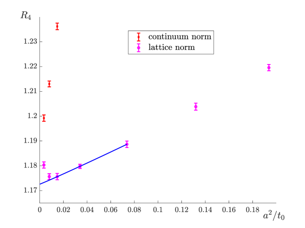
Figure 1: Lattice dependence of $R_{4}=\overline{\mathcal{M}}_{4}/[\overline{\mathcal{M}}_{4}]_{g=0}$, where the normalization is performed with $[\overline{\mathcal{M}}_{4}]_{g=0}$ at finite $a$ (“lattice norm”) or at $a=0$ (“continuum norm”). The quark mass is around the charm quark mass.

3 Derivation of the $a^{2}\log(aM)$ term in the free theory

In this and the following section we study the small $t$ behavior where mass-effects can be neglected and we first consider the contribution to $\mathcal{M}_{4}$ from a range $t_{1}\leq t\leq t_{2}\ll 1/M$,

$$\Delta I(t_{1},t_{2}) = 2a\sum_{t=t_{1}}^{t_{2}}w_{\mathrm{T}}(t)\,t^{4}\,G(t,M,a)-I_{\mathrm{cont}}(t_{1},t_{2})\,,\quad t_{1}M\ll 1,\;t_{2}M\ll 1\,,$$ (7)

$$I_{\mathrm{cont}}(t_{1},t_{2})=2\int_{t_{1}}^{t_{2}}\mathrm{d}t\;t^{4}\,G(t,M,0)\,,\quad t_{1}M\ll 1,\;t_{2}M\ll 1\,.$$

The weight $w_{\mathrm{T}}(t)$ implements the trapezoidal rule: it is $1/2$ at the boundaries and $1$ otherwise.

In order to gain understanding, we start with the free theory, $g=0$. This case is illuminating and at the same time we can get the relevant result by dimensional reasoning alone.

We split

$$\Delta I(0,t) = \Delta I(0,t_{1})+\Delta I(t_{1},t)\,,$$ (8)

discuss the second term and then add the first one. The SymEFT prediction for the cutoff effects of $G$ are

$$\Delta G = k_{\mathrm{L}}\,\frac{a^{2}}{t^{5}}+\mathrm{O}(a^{4})+\mathrm{O}(M^{2}t^{2})\,,$$ (9)

with a constant $k_{\mathrm{L}}$ which depends on the fermion discretization. Performing an explicit leading order computation, expanded in $a/t$ in the Wilson regularization we find $k_{\mathrm{L}}=1$. Since mass-effects are irrelevant, $k_{\mathrm{L}}=1$ holds irrespective of whether we choose a twisted mass term or a standard one. Not indicating the higher order corrections in $a$ and $M$ any further we get

$$\Delta I(t_{1},t) \overset{a\ll t_{1}}{\sim} \;k_{\mathrm{L}}\,a^{2}\ \,\int_{t_{1}}^{t}\,\mathrm{d}s\,s^{-1}+\Delta I_{\mathrm{T}}(t_{1},t)\,$$ (10)

$$= k_{\mathrm{L}}a^{2}\,\,\log(t/t_{1})+\Delta I_{\mathrm{T}}(t_{1},t)=k_{\mathrm{L}}a^{2}\,[\log(t/a)-\log(t_{1}/a)]+\Delta I_{\mathrm{T}}(t_{1},t)\,.$$ (11)

Here, $\Delta I_{\mathrm{T}}\sim a^{2}$ is the error in using the trapezoidal rule for the integral. We drop it because it does not play a role in the following; it is regular as $t\to 0$ and does not introduce a log. We then obtain

$$\Delta I(0,t) = \underbrace{\Delta I(0,t_{1})-k_{\mathrm{L}}a^{2}\log(t_{1}/a)}_{=k\,a^{2}}+k_{\mathrm{L}}\,a^{2}\,\log(t/a)=a^{2}\,[k+k_{\mathrm{L}}\log(t/a)]\,,$$ (12)

with another dimensionless constant $k$ depending on the regularization. The first term, $ka^{2}$, has this form because it neither depends on $t_{1}$ nor on $t$ and $a$ is the only dimensionful parameter.

For the full moment, $t$ gets replaced by the only physics scale of the integral, namely $1/M$. We thus arrive at

$$\frac{\Delta\mathcal{M}_{4}(M,a)}{\mathcal{M}_{4}(M,0)} = a^{2}M^{2}\,[k^{\prime}-k_{\mathrm{L}}\log(M\,a)]+\mathrm{O}(M^{4}a^{4})\,\,.$$ (13)

We note that [11] have argued for the presence of a $\log(t/a)$ term in the same discretised integral (in the context of HVP). In contrast to their argumentation, we never work with divergent integrals or with the Symanzik expansion for $a/t=\mathrm{O}(1)$.

It is instructive to add higher order terms, $k_{d}\,(a^{2}/t^{5})\,(a/t)^{d-2}$ with $d>2$ terms in the SymEFT for $\Delta G$. They yield

$$\Delta I(t_{1},t) \overset{a\ll t_{1}}{\sim} \;k_{\mathrm{L}}a^{2}\,[\log(t/a)-\log(t_{1}/a)]+a^{2}\sum_{d>2}\frac{k_{d}}{d-2}\,[\,(a/t_{1})^{d-2}-(a/t)^{d-2}\,]\,.$$ (14)

and

$$\Delta I(0,t) \sim \;a^{2}k^{\prime\prime}\,+\,k_{\mathrm{L}}a^{2}\,\log(t/a)-a^{2}\sum_{d>2}\frac{k_{d}}{d-2}(a/t)^{d-2}\,,$$ (15)

where $k^{\prime\prime}$ now receives contributions also from the $d>2$ terms in $\Delta G$. Note that the reasoning for the term $a^{2}k^{\prime}$ is unchanged. It is simply the dimension of $\Delta I$ inherited from the one of $I$ and the independence on $t_{1}$. This means that Symanzik improvement does not hold for the integral: we could improve $\Delta G$ such that all $\sim a^{2}$ terms are removed, but $\Delta\mathcal{M}_{4}$ would remain of order $a^{2}$ due to the $d>2$ terms in (14). "Only" the log-term at order $a^{2}$ disappears by improvement of the integrand.

Consider for a moment the moment

$$N_{3}=a\sum_{t\geq 0}t^{3}\,G(t,M,a)\,.$$ (16)

In this case, we obtain $\mathrm{O}(a)$ effects, irrespective of how the theory was improved. It is relevant to investigate whether such terms appear in some (sub-)integrals in representations of light-by-light scattering evaluated on the lattice [12].

4 SymEFT analysis beyond the free theory

It is not difficult to follow the above steps for the interacting theory. One has to write $\Delta G$ as in eq. 4 and also the short distance behavior changes due to anomalous dimension effects. These modifications introduce powers of $\alpha_{s}(1/a)$ and $\alpha_{s}(1/t)$, respectively, but are not of prime relevance. More important is that the step analogous to eq. 12 is modified to

$$ka^{2}\to K(a\Lambda)\,a^{2}\,,$$ (17)

with a function $K(a\Lambda)$ which is not restricted by simple arguments. Without knowing the behavior of $K$ at the origin, nothing can be concluded about $M$-independent $a$-effects of the integral. The structure of external scale dependent cutoff effects will be discussed in a publication [13]. The basic reason for the difficulty is of course that the interacting theory has a dynamical scale, $\Lambda$, which makes the dimensional analysis much less restrictive.

5 Higher moments $\mathcal{M}_{n},\;n>4$

With $n>4$, the $a^{2}\log(aM)$ term is absent in the free theory. Still, $\log(aM)$ dependences are present, but they are pushed to a higher order in $a$,

$$\mathcal{M}_{n}=\ldots+\mathrm{const.}\,\times a^{n-2}\log(aM)+\ldots\,.\qquad$$ (18)

6 Solutions

Our discussion shows that integrals of the considered type cannot be computed on the lattice in the straight-forward way. The best solution to this problem is to avoid integrands which have a behavior $\sim t^{k}\,,k<2$. First we describe a specific solution for $\overline{\mathcal{M}}_{4}$ for which we have a complete numerical demonstration. Then we propose a general solution, which in particular will be useful for HVP.

6.1 A practical solution for $\overline{\mathcal{M}}_{4}$

Our simple solution for the moment $\overline{\mathcal{M}}_{4}$ uses two different masses in the form (dropping the $a$-dependence)

$$\rho(M_{1},M_{2}) =\frac{2\pi^{2}}{3}\,(1-r^{2})^{-1}\,[\overline{\mathcal{M}}_{4}(M_{1})-r^{2}\overline{\mathcal{M}}_{4}(M_{2})]$$ (19)

$$=\frac{2\pi^{2}}{3}\,(1-r^{2})^{-1}M_{1}^{2}[\mathcal{M}_{4}(M_{1})-\mathcal{M}_{4}(M_{2})]\,,\quad r=M_{1}/M_{2}>1.$$ (20)

The second line shows that the small $t$ asymptotics of the integrand is improved via,

$$t^{4}\,[G(t,M_{1})-G(t,M_{2})]\sim t^{4}\,(t^{2}M_{2}^{2}-t^{2}M_{1}^{2})+\mathrm{O}(t^{8})\,.$$ (21)

There are log-corrections to this equation in the interacting theory, which are not relevant here. Due to the extra two powers of $t$, which come with the mass-effects, the quantity $\rho(M_{1},M_{2})$ has no log-enhanced $a^{2}$ effects (they will appear only at the level $a^{4}$).

For the purpose of extracting $\alpha_{s}$ it is now relevant to choose $M_{1}$ and $M_{2}$ not too different. Then the perturbative expansion, which is given in terms of the one of $\overline{\mathcal{M}}_{4}$, does not contain large logs of $M_{2}/M_{1}$. We write the perturbative expansion in terms of $\alpha_{s}(m_{2\star})$ with $M_{1}>M_{2}$. The $\frac{2\pi^{2}}{3}\,(1-r^{2})^{-1}$ normalization in eq. 19 ensures

$$\rho(M_{1},M_{2})=1+c_{1}\alpha_{\rm\overline{MS}}(m_{2\star})+\ldots\,,$$ (22)

where $c_{1}=0.74272...$ is the same expansion coefficient as the one of $R_{4}=\frac{2\pi^{2}}{3}\overline{\mathcal{M}}_{4}$ and higher order ones are easily obtained. We expand in $\alpha_{\rm\overline{MS}}(m_{2\star})$ because the difference is dominated somewhat more by long distances and $M_{2}$ is the smaller of the masses.

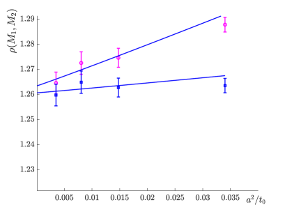
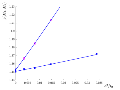
Figure 2: Continuum limit extrapolations of $\rho$ and its TL improved version, $\rho(M_{1},M_{2})^{\mathrm{Latnorm}}$. Masses, specified in units $z_{i}=M_{i}\sqrt{8t_{0}}$, are $z_{1}=4.5,\;z_{2}=3$ (left) and $z_{1}=13.5,\;z_{2}=9$ (right).

We show continuum limit extrapolations in fig. 2. They are almost straight in $a^{2}$ at small $a$ which makes them quite easy to do. They can be further improved by dividing $\rho$ by the same function evaluated at leading order, i.e. $g=0$. There is a choice which masses to insert into the leading order formula. A good choice is again $m_{\star}$. Precisely we define

$$R_{4}^{\mathrm{TL}}(a\mu)=R_{4}|_{g=0}$$ (23)

with $\mu$ the twisted mass and then

$$\rho^{\mathrm{Latnorm}}(M_{1},M_{2}) = \frac{3}{2\pi^{2}}\,(1-r_{\star}^{2})\,\frac{\rho(M_{1},M_{2})}{R_{4}^{\mathrm{TL}}(am_{\star 1})-r_{\star}^{2}R_{4}^{\mathrm{TL}}(am_{\star 2})}$$ (24)

with

$$r_{\star}=\frac{m_{\star 1}}{m_{\star 2}}\,.$$ (25)

In principle it is important that $r_{\star}$ is given by the ratio of the masses that appear in $R_{4}^{\mathrm{TL}}$ for the log-term to cancel. But numerically, replacing $r_{\star}\to r$ makes only a small difference. Examples for how the discretization errors are reduced can be seen in fig. 2. For all our values of $M_{1},M_{2}$, the leading order improved $\rho(M_{1},M_{2})^{\mathrm{Latnorm}}$ has a rather convincing continuum extrapolation.

After the continuum extrapolation, one straight-forwardly extracts the effective $\Lambda$-parameter and arrives at the red circles in fig. 3. These values are computed from three-loop perturbation theory (i.e. including $\alpha^{3}$ in $R_{4}$) at finite $\alpha(m_{\star})$. They then have a residual dependence

$$\Lambda_{\mathrm{eff}}=\Lambda+\mathrm{O}(\alpha^{2}(m_{\star}))\,,$$ (26)

on $m_{\star}$ and we call them “effective”. The comparison to the Dalla Brida and Ramos value [14], extracted at $\alpha^{2}<0.01$ with the help of a finite size step scaling method, shows that $\Lambda$ computed from $\rho$ has at most small (on the scale of our uncertainties) corrections at the largest mass. That mass is given by $z=9$ or $m_{\star}\approx 2.7\,\mathrm{GeV}$.

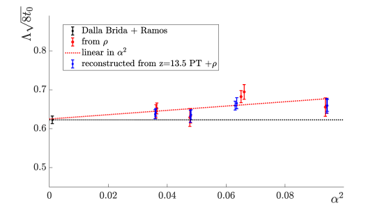
Figure 3: $\Lambda_{\rm\overline{MS}}$ computed from $\alpha_{\rm\overline{MS}}(m_{2\star})$, where the latter is obtained from the non-perturbative $\rho$. The dotted line is a fit to all points including the Dalla Brida / Ramos one [14]. The reconstructed data points are described in the text.

6.2 Reconstruction of $R_{4}=\frac{2\pi^{2}}{3}\overline{\mathcal{M}}_{4}(M)$ from $\rho$.

From the definition eq. 19 of $\rho$ it is clear that given $\rho(M_{1},M_{2})$ and $R_{4}(M_{2})$ one can determine $R_{4}(M_{1})$. This can be exploited by using $\rho$ to go from $R_{4}(M_{\mathrm{ref}}\gg\Lambda)$, where perturbative uncertainties are suppressed the most, to smaller masses. We insert the known [14] $\Lambda$-parameter into the three-loop (i.e. including $\alpha^{3}$) perturbative expression for $R_{4}$ at our highest mass, $z_{\mathrm{ref}}=13.5$ and obtain

$$R_{4}^{\mathrm{reconstructed}}(M) = (1-r^{-2})\,\rho(M,M_{\mathrm{ref}})+r^{-2}\,R_{4}^{\mathrm{3-loop}}(M_{\mathrm{ref}})\,,\;$$ (28)

$$r=M/M_{\mathrm{ref}},\;z_{\mathrm{ref}}=\sqrt{8t_{0}}M_{\mathrm{ref}}=13.5\,.$$

Note that perturbative errors are small in $R_{4}(M_{\mathrm{ref}})$ as seen in the analysis of $\rho$. They get further suppressed by a factor $r^{-2}\approx 1/20$ when we go to $z=3$. This means that we obtain the non-perturbative dependence of $\Lambda_{\mathrm{eff}}$ (as of now computed from $R_{4}$ and therefore with somewhat different $\mathrm{O}(\alpha^{2})$ terms) on $\alpha$. We remind the reader that a direct computation of $R_{4}$ was impossible due to the $a^{2}\log(aM)$ effects.

6.3 Proposal for the HVP contribution to the muon $g-2$

The discussion in the previous section is easily transferred to the case of the muon $g-2$, working with differences of the HVP integral for different (artificial) muon masses. Additionally, we would like to advocate a very simple solution for this and similar cases, where the short distance contribution to the integral is subdominant. In contrast to the $\mathcal{M}_{4}$-case the goal is not to determine $\alpha_{s}$ or other short-distance parameters.

It is then advisable to split the integral into a short-distance part evaluated by continuum perturbation theory and a long-distance one to be computed on the lattice:

$$\int_{0}^{\infty}\mathrm{d}tF(t)=\underbrace{\int_{0}^{\infty}\mathrm{d}t\,[1-\chi(t)]\,F(t)}_{\text{continuum PT}}\,+\,\underbrace{a\sum_{t=0}^{\infty}\,\chi(t)\,\,F(t)}_{\text{continuum limit of lattice results}}\,,\quad\chi(t)\,\sim\,\begin{cases}\mathrm{O}(t^{2})&t\Lambda_{\mathrm{\overline{MS}}}\ll 1\\ 1&t\Lambda_{\mathrm{\overline{MS}}}\gg 1\end{cases}\,.$$ (29)

For example the function $\chi$ can be taken as

$$\chi(t)=\frac{(M_{\mathrm{cut}}t)^{k}}{(M_{\mathrm{cut}}t)^{k}+1}\,,\;M_{\mathrm{cut}}\gg\Lambda_{\mathrm{\overline{MS}}}$$ (30)

or also as a step-function, $\chi(t)=\theta(tM_{\mathrm{cut}}-1)$. The smooth version seems advantageous for perturbation theory as well as for the lattice discretization of the integral. The use of perturbation theory for the small $t$-part of the integral has already been anticipated in [2]. Our discussion adds further motivation and understanding. It suggests a smooth function $\chi$ such as eq. 30.
Acknowledgements. We thank the organizers for a very pleasant and successful conference. Discussions with H. Meyer, S. Kuberski and A. Risch on HVP are gratefully acknowledged. We also thank C. Lehner for an email exchange on that subject. LC and RS acknowledge funding from the European Union’s Horizon 2020 research and innovation programme under the Marie Skłodowska-Curie grant agreement No. 813942.

References

• [1] HPQCD collaboration, High-Precision Charm-Quark Mass and QCD coupling from Current-Current Correlators in Lattice and Continuum QCD, Phys. Rev. D 78 (2008) 054513 [0805.2999].
• [2] D. Bernecker and H.B. Meyer, Vector Correlators in Lattice QCD: Methods and applications, Eur. Phys. J. A 47 (2011) 148 [1107.4388].
• [3] K. Symanzik, Continuum limit and improved action in lattice theories:(i). principles and $\varphi$4 theory, Nuclear Physics B 226 (1983) 187.
• [4] N. Husung, P. Marquard and R. Sommer, Asymptotic behavior of cutoff effects in Yang–Mills theory and in Wilson’s lattice QCD, Eur. Phys. J. C 80 (2020) 200 [1912.08498].
• [5] N. Husung, Logarithmic corrections to O($a$) and O($a^{2}$) effects in lattice QCD with Wilson or Ginsparg-Wilson quarks, 2206.03536.
• [6] L. Chimirri and R. Sommer, Investigation of the Perturbative Expansion of Moments of Heavy Quark Correlators for $N_{f}=0$, PoS LATTICE2021 (2022) 354 [2203.07936].
• [7] N. Husung, M. Koren, P. Krah and R. Sommer, SU(3) Yang Mills theory at small distances and fine lattices, EPJ Web Conf. 175 (2018) 14024 [1711.01860].
• [8] B. Sheikholeslami and R. Wohlert, Improved Continuum Limit Lattice Action for QCD with Wilson Fermions, Nucl. Phys. B 259 (1985) 572.
• [9] M. Lüscher, S. Sint, R. Sommer, P. Weisz and U. Wolff, Nonperturbative O(a) improvement of lattice QCD, Nucl. Phys. B 491 (1997) 323 [hep-lat/9609035].
• [10] L. Chimirri and R. Sommer, A quenched exploration of heavy quark moments and their perturbative expansion, 2023.
• [11] T. Harris, M. Cè, H.B. Meyer, A. Toniato and C. Török, Vacuum correlators at short distances from lattice QCD, PoS LATTICE2021 (2021) 572 [2111.07948].
• [12] E.-H. Chao, R.J. Hudspith, A. Gérardin, J.R. Green, H.B. Meyer and K. Ottnad, Hadronic light-by-light contribution to $(g-2)_{\mu}$ from lattice QCD: a complete calculation, Eur. Phys. J. C 81 (2021) 651 [2104.02632].
• [13] L. Chimirri, N. Husung and R. Sommer, in preparation, 2023.
• [14] M. Dalla Brida and A. Ramos, The gradient flow coupling at high-energy and the scale of SU(3) Yang–Mills theory, Eur. Phys. J. C 79 (2019) 720 [1905.05147].