Hard X–ray Observations of the Hydrogen-poor Superluminous Supernova with

Abstract

Some Hydrogen-poor superluminous supernovae are likely powered by a magnetar central engine, making their luminosity larger than common supernovae. Although a significant amount of X–ray flux is expected from the spin down of the magnetar, direct observational evidence is still to be found, giving rise to the “missing energy” problem. Here we present observations of nearby SN 2018hti (catalog ) 2.4 y (rest frame) after its optical peak. We expect that, by this time, the ejecta have become optically thin for photons more energetic than $\sim 15$ keV. No flux is detected at the position of the supernova down to $F_{\rm{10-30keV}}=9.0\times 10^{-14}$ erg cm^-2 s^-1, or an upper limit of $7.9\times 10^{41}$ erg s^-1 at a distance of 271 Mpc. This constrains the fraction of bolometric luminosity from the putative spinning down magnetar to be $f_{\rm X}\lesssim 36\%$ in the 10–30 keV range in a conservative case, $f_{\rm X}\lesssim 11\%$ in an optimistic case.

1 Introduction

Explosions from the core collapse of massive stars generate supernovae (SNe) with a broad range of peak luminosities, but typically falling below $10^{43}\rm\,erg\,s^{-1}$. Superluminous supernovae (SLSNe) are a rare class of stellar explosions with peak luminosities $>7\times 10^{43}$ erg s^-1 (Gal-Yam, 2019), which is $>10\times$ more luminous than typical core-collapse SNe. Optical surveys have shown that the volumetric rate of SLSNe is of the order of $1\%$ of the SN population (Fremling et al., 2020).

Interaction between the ejecta and circumstellar material is likely responsible for the large luminosity of Hydrogen-rich (Type II) SLSNe. However, hydrogen-poor SLSNe (Type I, or SLSN-I) likely involves a different mechanism, the leading candidate is a highly magnetized neutron star that continuously spins down and pumps energy into the ejecta (Kasen & Bildsten, 2010; Woosley, 2010; Metzger et al., 2014).

The magnetar model fits the SLSN-I light curves well up to $\sim 100$ days from the explosion, when the spectral energy distribution (SED) peaks at optical/UV wavelengths. At later times, the spin-down luminosity of the magnetar exceeds the optical luminosity and the model needs to be modified to allow the majority of the spin-down energy to directly leak out of the ejecta. Some evidence of late-time excess $\sim 800$ days past explosion was found with deep optical observations for SN 2016inl (Blanchard et al., 2021). However, the anticipated large amount of leaked energy, about $10^{50}$ to $10^{51}\rm\,erg$, has so far gone undetected (Bhirombhakdi et al., 2018; Margutti et al., 2018).

Follow-up campaigns of nearby SLSNe (Bhirombhakdi et al., 2018; Margutti et al., 2018) were conducted in the soft X-ray band with XMM-Newton, Chandra, and the Neil Gehrels Swift Observatory, placing deep constraints on the emission between 0.3 keV and 10 keV. Only one faint counterpart was found for PTF12dam (Margutti et al., 2018), but the flux was consistent with the underlying star forming activity in the host galaxy and the X-rays may not be from the SLSN source. As we demonstrate in Equation 3, the non-detection in soft X–rays may be explained by the large bound-free optical depth of the ejecta. In the high-energy $\gamma$-ray ($\gtrsim 1\rm\,GeV$) band, Fermi LAT observations placed constraints on the luminosity $L_{\rm GeV}\lesssim 10^{42}\rm\,erg/s$ on a timescale of a few years after the explosion (Renault-Tinacci et al., 2018). Thus, the question remains open: where is the missing energy? And what percentage of it is emitted in the X-ray band?

The Nuclear Spectroscopic Telescope Array (; Harrison et al., 2013) offers the possibility to address these outstanding questions by measuring the fraction of the missing energy emitted in the 3–79 keV range a few years after the explosion when the ejecta have become optically thin in the hard X–ray band.

Among the Hydrogen-poor SLSNe present in public catalogs (such as the Transient Name Server and the Open Supernova Catalog) in early 2021, we deemed  particularly promising to be detected with .  was discovered by the Asteroid Terrestrial-impact Last Alert System (ATLAS; Tonry et al., 2018) on 2018-11-02 at coordinates RA $=$ 03^h40^m53.760^s; Dec $=$ +11${\degree}$46^′37.38^′′ (J2000). The transient was then classified as a SLSN-I (Burke et al., 2018) at redshift $z=0.0614$ (Fiore et al., 2022). Follow-up observations and modeling for  are presented in Lee (2019); Lin et al. (2020); Fiore et al. (2022).

The paper is organized as follows. We present  observations of  and data analysis method in §2, the analysis results in §3, a discussion on the implications for the missing energy problem in §4, and our conclusions in section §5. Times are UT throughout the manuscript.

2 Observations and data analysis

was observed with in two epochs at the beginning of  GO Cycle 7 (proposal 7264; P.I. Andreoni). The first epoch (ID 40701008001) started on 2021-07-01 16:34, with an exposure time of 101,690 s. The second epoch (ID 40701008002) started on 2021-07-06 18:57, with an exposure time of 53,887 s.

Data were reduced using HEASoft v.6.29 and the NuSTAR Data Analysis Software (NuSTARDAS) v.2.1.1, in particular the nupipeline and nuproducts routines. South Atlantic Anomaly (SAA) effects on the background were mitigated using the nucalcsaa routine.

The first epoch was significantly affected by solar activity outside the SAA. To mitigate the background increase, we extracted a light curve of an empty background region ($r=100^{\prime\prime}$), binned by 100 s bins and we identified those time intervals in which the rate exceeded the median rate by $3\times$ the standard deviation of the rates. We repeated this process twice and excluded the affected time frames from the “good time interval” (GTI). After this operation, the effective exposure times became of 98.4 ks (FPMA) and 98.8 ks (FPMB). The total exposure time resulting from both epochs and both FPMA and FPMB instruments was $t_{\rm{exp}}=302.4$ ks.

The upper limits on the flux presented below (§3) were obtained using the X–ray spectral fitting package XSpec (Arnaud, 1996) of the HEAsoft software suite (NASA High Energy Astrophysics Science Archive Research Center (2014), Heasarc).

3 Results

We performed photometry using a circular aperture with radius $r=40^{\prime\prime}$, which is large enough to account for small ($<10^{\prime\prime}$) offsets possibly present in the astrometric calibration. The background region was chosen in the same detector where  was expected to be found and had a radius of $r=100^{\prime\prime}$. Our observations did not reveal any source at the location of (Fig. 1).

We focused our analysis in the 10–30 keV range because the SN is expected to be optically thick at energies below $\sim 10$ keV (see §4) and too faint to be detectable at energies above $\sim 30$ keV because of the lower effective area. We obtained an upper limit of $2.4\times 10^{-4}$ counts s^-1. This was calculated as $3\times\sqrt{B_{\rm tot}}/t_{\rm{exp}}$, where $B_{\rm tot}$ is the total background from both epochs and both instruments normalized to the source aperture and $t_{\rm{exp}}$ is the total exposure time.

Assuming a power-law model with photon index $\Gamma=2$ normalized to match the expected count rate, this corresponds to an unabsorbed flux of $F_{\rm{10-30keV}}=5.4\times 10^{-14}$ erg cm^-2 s^-1 in the 10–30 keV range, or an upper limit of $4.8\times 10^{41}$ erg s^-1 at a luminosity distance of 271 Mpc (Fiore et al., 2022). We defined a multiplicative absorption factor $e^{-\tau(E)}$ in XSpec, with $\tau(E)$ defined as in Eq. 3. The resulting flux with absorption from the ejecta taken into account is $F_{\rm{10-30keV}}=9.0\times 10^{-14}$ erg cm^-2 s^-1, which leads to an upper limit of $7.9\times 10^{41}$ erg s^-1 at a luminosity distance of 271 Mpc. The result is shown in Fig. 2.

We note that this luminosity upper limit is independent of the assumption on the neutral hydrogen column density $N_{\rm H}$ in the interstellar medium of the host galaxy and the Milky Way, because the 10–30 keV flux only gets significantly attenuated by the interstellar medium for $N_{\rm H}\gtrsim 10^{24}\rm\,cm^{-2}$ (Wilms et al., 2000), which is unlikely given that the source is observed in the optical band.

During the analysis, a new source was found serendipitously in the field (Fig. 3). The source is located at coordinates RA $=$ 03^h41^m21^s; Dec $=$ +11${\degree}$48^′29^′′ ($\sim 30^{\prime\prime}$ error radius). One cataloged AGN candidate, WISEA J034122.85+114833.2, is located $27.6^{\prime\prime}$ away from the position, close to the edge of the error region, so an association between the two sources cannot be excluded. Follow-up observations to determine its nature are planned. Since this source was found on a different detector than , its presence did not affect our SN analysis.

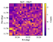
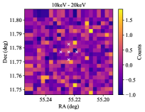
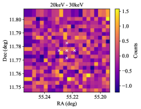
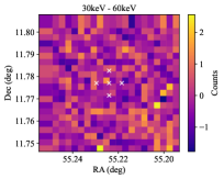
Figure 1: Stacked, background-subtracted photometry of in four energy ranges obtained using a grid of $10^{\prime\prime}\times 10^{\prime\prime}$ squared apertures. Each image has sides of $200^{\prime\prime}$ and is oriented with North to the top and East to the left. White crosses guide the eye by indicating the expected location of and $20^{\prime\prime}$ separations in both directions.

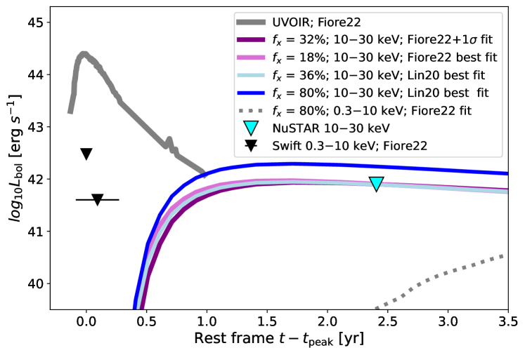
Figure 2: The upper limit in the 10–30 keV range is shown (cyan triangle; $L_{\rm bol}<7.9\times 10^{41}$ erg s^-1) along with the pseudo-bolometric light curve (grey line; Fiore et al., 2022) and $Swift$ upper limits (black triangles; Fiore et al., 2022). The X–ray emission expected from magnetar spin-down is presented using the magnetic field and ejecta mass resulting from the fit performed by Lin et al. (2020) and Fiore et al. (2022) for several values of $f_{\rm X}$. We represented the model using the best fit values for $B$ and $M_{\rm ej}$ for Fiore et al. (2022) (Fiore22 best fit) as well as the best values plus the 1$\sigma$ uncertainty in the parameter estimation (Fiore22$+1\sigma$ fit). Models brighter than the   upper limit are excluded by our observations (see §4), for example the model that assumes the Lin et al. (2020) best fit parameters and a large $f_{X}=80\%$ (blue solid line). The emission expected in the 0.3–10 keV range, in which the ejecta should still be optically thick, is represented with a dotted line for comparison.

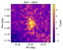
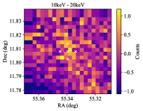
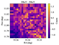
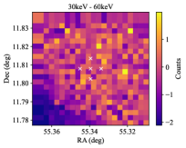
Figure 3: Images of an X–ray source serendipitously observed in the field, obtained as those in Fig. 1.

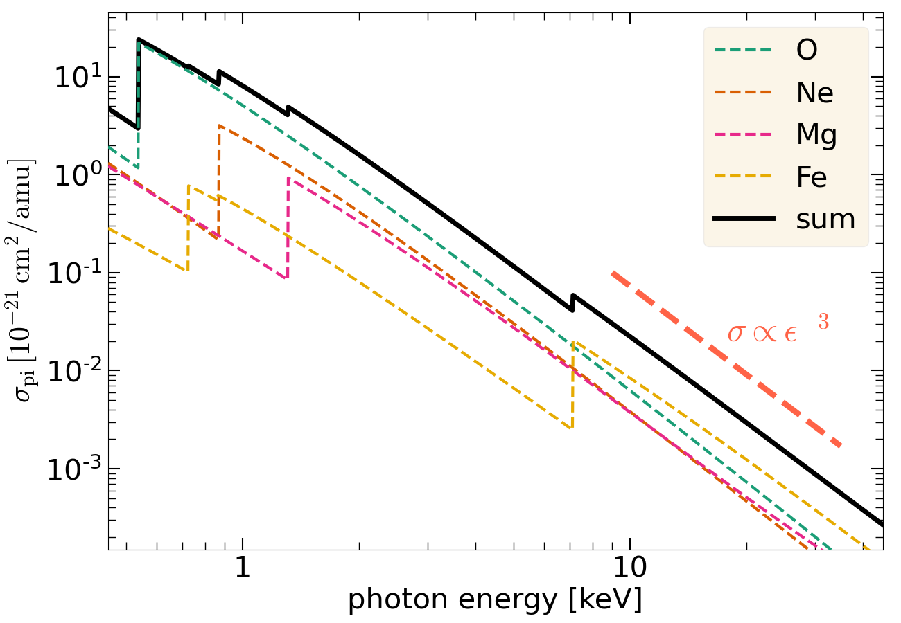
Figure 4: Photo-ionization opacity (in units of $\rm cm^{2}$ per atomic mass unit) for a model ejecta with abundance mass ratio of $\rm O:Ne:Mg:Fe=0.76:0.15:0.07:0.02$. The thick black line shows the total opacity and the dashed lines show contributions from different species. For this composition, the bound-free opacity is dominated by O and Fe.

4 Discussion

To obtain a good fit to the late-time ($>100$ days) optical light curve, magnetar models have been developed by Chen et al. (2015); Wang et al. (2015) to allow the magnetar spin-down luminosity to leak out of the ejecta. Such a model has been used to fit the multi-color light curves of a large number of SLSNe-I, and the authors in Nicholl et al. (2017); Lin et al. (2020) provided the Bayesian posteriors of the magnetic field strength $B$ and ejecta mass $M_{\rm ej}$.The characteristic ejecta velocity $v_{\rm ej}$ is approximated by the photospheric expansion velocity inferred from the absorption line widths (Liu et al., 2017), and typical values are $v_{\rm ej}\simeq 1\times 10^{4}\mathrm{\,km\,s^{-1}}$. Using the same framework as in Nicholl et al. (2017), we expect the magnetar heating luminosity at late time ($t\gtrsim 1\rm\,yr$) to be

$$L_{\rm mag}\simeq 3.4\times 10^{42}\mathrm{\,erg\,s^{-1}}\,(B/10^{14}\mathrm{G})^{-2}(t/\mathrm{yr})^{-2}.$$ (1)

In the hard X-ray band, the absorption opacity of the SN ejecta is dominated by bound-free ionization of K-shell electrons. Without a generally accepted progenitor model for SLSNe-I (see Moriya et al., 2018, for a review of the proposed models), their ejecta abundances are only weakly constrained by spectroscopic observations so far. Throughout the evolution, SLSN-I spectra show absorption and emission lines of C, O, Na, Mg, Si, Ca, Fe in low ionization states, and their nebular spectra resemble those of Type Ic SNe such as SN1998bw (Jerkstrand et al., 2017; Nicholl, 2021). Models (Dessart et al., 2012; Mazzali et al., 2016; Jerkstrand et al., 2017) that produce a reasonable fit to the observed spectra generally have ejecta masses dominated by O, Ne, Mg (products of C-burning). Since the magnetar models that fit the lightcurves usually do not require heating from $\rm{}^{56}Ni$ decay, the mass of the Fe-group elements may be small (although it is only weakly constrained). Thus, we expect the bound-free opacity in the hard X-ray band to be dominated O, Ne, Mg as well as Fe if the explosions produce a substantial $\rm{}^{56}Ni$ mass $M_{\rm Ni}\gtrsim 0.1M_{\odot}$. To estimate the ejecta opacity, we take a fiducial abundance profile based on C-burning ashes of a $25M_{\odot}$ massive star from Jerkstrand et al. (2017); Woosley & Heger (2007) and then added 2% of iron (corresponding to $M_{\rm Ni}$ of the order $0.1M_{\odot}$) to obtain the final mass ratio of $\rm O:Ne:Mg:Fe=0.76:0.15:0.07:0.02$. A higher Fe mass fraction would give larger bound-free opacity in the hard X-ray band and hence our constraint on the hard X-ray luminosity from the central engine would be weaker.

The bound-free opacity according to our fiducial abundance profile, as computed using the analytic fits for the photoionization cross-sections for neutral atoms (Verner & Yakovlev, 1995; Verner et al., 1996), is shown in Fig. 4 and is analytically given by (for photon energy $E\gtrsim 10\rm\,keV$)

$$\kappa_{\rm bf}(E)\simeq 11\,\left(E\over{\rm 10\,keV}\right)^{-3}\,\mathrm{cm^{2}\,g^{-1}}.$$ (2)

Therefore, the absorption optical depth of the ejecta when it is at a radius $r=v_{\rm ej}t$ at time $t$ since explosion is given by

$$\begin{split}&\tau(E)\simeq{3\kappa_{\rm bf}M_{\rm ej}\over 4\pi(v_{\rm ej}t)^{2}}\\ &\simeq 4.5\,\left(E\over 10{\rm\,keV}\right)^{-3}{M_{\rm ej}\over 5M_{\odot}}\left(v_{\rm ej}\over 10^{4}\,\mathrm{km\,s^{-1}}\right)^{-2}\left(t\over 2.4\,\mathrm{yr}\right)^{-2}.\end{split}$$ (3)

This means that the ejecta may be optically thick to soft X–rays for decades, but hard X-rays $\gtrsim 10\,$keV may escape a few years after the explosion, while the magnetar luminosity is still high (see Eq. 1).

To constrain the fraction of the missing energy in the hard X–rays, we assumed that a fraction $f_{\rm X}=L_{\rm{10\mbox{--}30\,keV}}/L_{\rm mag}$ of the bolometric luminosity expected from the spinning down magnetar is emitted as a power-law in the 10–30 keV band, probed by , and that the photon index is $\Gamma=2$. From a theoretical point of view, this fraction $f_{\rm X}$ is highly uncertain. The radiation spectrum of the magnetar wind nebula depends on how particles are accelerated near the wind termination shock (located at the inner edge of the SN ejecta), the competition between synchrotron and inverse-Compton cooling of the shock-accelerated particles, as well as photon-photon pair production (Metzger et al., 2014; Vurm & Metzger, 2021).

No X–ray flux from the SLSN central engine was revealed by these  observations, however we can constrain $f_{X}$. Using the magnetic field and ejecta mass inferred by Lin et al. (2020), $B=1.8\times 10^{13}$ G and $M_{\rm{ej}}=5.8$ M_⊙, the  upper limit of $7.9\times 10^{41}$ erg s^-1 leads to a constraint of $f_{\rm X}<0.36$ (Fig. 2). Fiore et al. (2022) obtained $B=1.3^{+0.3}_{-0.2}\times 10^{13}$ G, $M_{\rm{ej}}=5.2^{+1.4}_{-0.9}$ M_⊙, and a velocity $v_{\rm ej}=0.95\times 10^{4}\mathrm{\,km\,s^{-1}}$. The best fit values lead to a constraint of $f_{\rm X}<0.18$, more stringent that using the parameters obtained by Lin et al. (2020). When accounting for the 1$\sigma$ uncertainty in the parameter estimation (Fiore et al., 2022), upper limits of $f_{\rm X}<0.32$ ($B=1.6\times 10^{13}$ G, $M_{\rm{ej}}=6.6$ M_⊙) and $f_{\rm X}<0.11$ ($B=1.1\times 10^{13}$ G, $M_{\rm{ej}}=4.3$ M_⊙) can be inferred. In conclusion, an upper limit of $f_{\rm X}<0.36$ is conservative for the parameters taken from both Fiore et al. (2022) and Lin et al. (2020). Our constraints on $f_{X}$ are summarized in Tab. 1, where upper limits obtained without the absorption factor are also reported.

It is possible that only a fraction $f_{\rm r}<1$ of the spin-down power of the magnetar is converted into radiation which then heats the supernova ejecta — the rest of the spin-down power may go into pair creation, kinetic energy of the expansion, and escaping Poynting flux. If this is the case, then the heating luminosity is lower than in our Eq. (1), which is used in the fitting models under the assumption that the heat and spin-down luminosities are equal, by a factor of $f_{\rm r}^{-1}$.

Our final constraint is based on the heating luminosity $L_{\rm mag}(t=2.4\rm\,yr)$, which is a power-law ($t^{-2}$) extrapolation from the heating luminosity required to reproduce the optical lightcurve at earlier epochs.

In reality, if the bolometric radiative efficiency is time dependent in the first few years $f_{\rm r}(t)$, this time dependence should be included in the extrapolation. It is beyond the scope of this work to calculate $f_{\rm r}(t)$ for the magnetar wind in the first few years, but we note that in the model presented in Vurm & Metzger (2021), relativistic particles injected by the pulsar wind are in the fast cooling regime in the first few decades (see their Eq. 23), so the radiative efficiency $f_{\rm r}$ remains roughly constant in the first few years. It is straightforward to scale our constraint on $f_{\rm X}$ to alternative models where the heating luminosity has a different time dependence than the $t^{-2}$ power-law.

B	$M_{\rm ej}$	Comment	Reference	Upper Limit	Upper Limit
($10^{13}$ G)	(M⊙)			unabsorbed	absorbed
1.8	5.8	best fit	Lin et al. (2020)	$<22\%$	$<36\%$
1.3	5.2	best fit	Fiore et al. (2022)	$<11\%$	$<18\%$
1.6	6.6	best fit + 1$\sigma$	Fiore et al. (2022)	$<19\%$	$<32\%$
1.1	4.3	best fit - 1$\sigma$	Fiore et al. (2022)	$<7\%$	$<11\%$

Table 1: Upper limit on the fraction $f_{\rm X}$ of the bolometric luminosity expected from the spinning down magnetar, emitted in the 10–30 keV band, assuming negligible absorption (fifth column) and absorption with optical depth $\tau(E)$ as in Eq. 3 (sixth column). The upper limits on the 10–30 keV band that we obtained are $7.9\times 10^{41}$ erg s^-1 and $4.8\times 10^{41}$ erg s^-1 for the absorbed and unabsorbed case, respectively. The first column lists the magnetic field and the second column the ejecta mass obtained by model fitting by Lin et al. (2020) or Fiore et al. (2022) (fourth column).

5 Conclusion

We conducted  observations of hydrogen-poor with the goal of measuring the fraction of luminosity emitted in the hard X–rays assuming a magnetar central engine. Bound-free processes make the ejecta optically thick to soft X–rays, but we estimated that flux should leak out at energies $\gtrsim 15$ keV after $2.4$ yr from the explosion time of . However,  observations resulted in an upper limit on the flux of $F_{10-30\rm{keV}}=7.9\times 10^{41}$ erg s^-1 ($F_{10-30\rm{keV}}=4.8\times 10^{41}$ erg s^-1 without accounting for absorption by the ejecta) at a luminosity distance of 271 Mpc.

These results imply that the fraction of hard X–rays (10–30 keV range) is $f_{\rm{X}}\lesssim 36\%$ of the bolometric luminosity expected from a magnetar spin-down, considering the values obtained by the less stringent model for of magnetic field $B$ and ejecta mass $M_{\rm{ej}}$ (Fiore et al., 2022, see §4), $f_{\rm{X}}\lesssim 11\%$ for the most optimistic model, in which the SLSN is expected to be brighter. Our constraints on the high-energy spectrum of SLSNe provide important guidance in future modeling of magnetar wind nebulae, provided that they are indeed the central engine of these events.

References

- Arnaud (1996) Arnaud, K. A. 1996, in Astronomical Society of the Pacific Conference Series, Vol. 101, Astronomical Data Analysis Software and Systems V, ed. G. H. Jacoby & J. Barnes, 17
- Astropy Collaboration et al. (2013) Astropy Collaboration, Robitaille, T. P., Tollerud, E. J., et al. 2013, A&A, 558, A33, doi: 10.1051/0004-6361/201322068
- Astropy Collaboration et al. (2018) Astropy Collaboration, Price-Whelan, A. M., Sipőcz, B. M., et al. 2018, AJ, 156, 123, doi: 10.3847/1538-3881/aabc4f
- Bhirombhakdi et al. (2018) Bhirombhakdi, K., Chornock, R., Margutti, R., et al. 2018, ApJ, 868, L32, doi: 10.3847/2041-8213/aaee83
- Blanchard et al. (2021) Blanchard, P. K., Berger, E., Nicholl, M., et al. 2021, ApJ, 921, 64, doi: 10.3847/1538-4357/ac1b27
- Burke et al. (2018) Burke, J., Hiramatsu, D., Arcavi, I., et al. 2018, Transient Name Server Classification Report, 2018-1719, 1
- Chen et al. (2015) Chen, T. W., Smartt, S. J., Jerkstrand, A., et al. 2015, MNRAS, 452, 1567, doi: 10.1093/mnras/stv1360
- Dessart et al. (2012) Dessart, L., Hillier, D. J., Waldman, R., Livne, E., & Blondin, S. 2012, MNRAS, 426, L76, doi: 10.1111/j.1745-3933.2012.01329.x
- Fiore et al. (2022) Fiore, A., Benetti, S., Nicholl, M., et al. 2022, MNRAS, 512, 4484, doi: 10.1093/mnras/stac744
- Fremling et al. (2020) Fremling, C., Miller, A. A., Sharma, Y., et al. 2020, ApJ, 895, 32, doi: 10.3847/1538-4357/ab8943
- Gal-Yam (2019) Gal-Yam, A. 2019, ARA&A, 57, 305, doi: 10.1146/annurev-astro-081817-051819
- Harrison et al. (2013) Harrison, F. A., Craig, W. W., Christensen, F. E., et al. 2013, ApJ, 770, 103, doi: 10.1088/0004-637X/770/2/103
- Jerkstrand et al. (2017) Jerkstrand, A., Smartt, S. J., Inserra, C., et al. 2017, ApJ, 835, 13, doi: 10.3847/1538-4357/835/1/13
- Kasen & Bildsten (2010) Kasen, D., & Bildsten, L. 2010, ApJ, 717, 245, doi: 10.1088/0004-637X/717/1/245
- Lee (2019) Lee, C.-H. 2019, ApJ, 875, 121, doi: 10.3847/1538-4357/ab113c
- Lin et al. (2020) Lin, W. L., Wang, X. F., Li, W. X., et al. 2020, MNRAS, 497, 318, doi: 10.1093/mnras/staa1918
- Liu et al. (2017) Liu, Y.-Q., Modjaz, M., & Bianco, F. B. 2017, ApJ, 845, 85, doi: 10.3847/1538-4357/aa7f74
- Margutti et al. (2018) Margutti, R., Chornock, R., Metzger, B. D., et al. 2018, ApJ, 864, 45, doi: 10.3847/1538-4357/aad2df
- Mazzali et al. (2016) Mazzali, P. A., Sullivan, M., Pian, E., Greiner, J., & Kann, D. A. 2016, MNRAS, 458, 3455, doi: 10.1093/mnras/stw512
- Metzger et al. (2014) Metzger, B. D., Vurm, I., Hascoët, R., & Beloborodov, A. M. 2014, MNRAS, 437, 703, doi: 10.1093/mnras/stt1922
- Moriya et al. (2018) Moriya, T. J., Sorokina, E. I., & Chevalier, R. A. 2018, Space Sci. Rev., 214, 59, doi: 10.1007/s11214-018-0493-6
- NASA High Energy Astrophysics Science Archive Research Center (2014) (Heasarc) NASA High Energy Astrophysics Science Archive Research Center (Heasarc). 2014, HEAsoft: Unified Release of FTOOLS and XANADU. http://ascl.net/1408.004
- Nicholl (2021) Nicholl, M. 2021, Astronomy and Geophysics, 62, 5.34, doi: 10.1093/astrogeo/atab092
- Nicholl et al. (2017) Nicholl, M., Guillochon, J., & Berger, E. 2017, ApJ, 850, 55, doi: 10.3847/1538-4357/aa9334
- Renault-Tinacci et al. (2018) Renault-Tinacci, N., Kotera, K., Neronov, A., & Ando, S. 2018, A&A, 611, A45, doi: 10.1051/0004-6361/201730741
- Tonry et al. (2018) Tonry, J. L., Denneau, L., Heinze, A. N., et al. 2018, Publications of the Astronomical Society of the Pacific, 130, 064505. http://stacks.iop.org/1538-3873/130/i=988/a=064505
- Verner et al. (1996) Verner, D. A., Ferland, G. J., Korista, K. T., & Yakovlev, D. G. 1996, ApJ, 465, 487, doi: 10.1086/177435
- Verner & Yakovlev (1995) Verner, D. A., & Yakovlev, D. G. 1995, A&AS, 109, 125
- Vurm & Metzger (2021) Vurm, I., & Metzger, B. D. 2021, arXiv e-prints, arXiv:2101.05299. https://arxiv.org/abs/2101.05299
- Wang et al. (2015) Wang, S. Q., Wang, L. J., Dai, Z. G., & Wu, X. F. 2015, ApJ, 799, 107, doi: 10.1088/0004-637X/799/1/107
- Wilms et al. (2000) Wilms, J., Allen, A., & McCray, R. 2000, ApJ, 542, 914, doi: 10.1086/317016
- Woosley (2010) Woosley, S. E. 2010, ApJ, 719, L204, doi: 10.1088/2041-8205/719/2/L204
- Woosley & Heger (2007) Woosley, S. E., & Heger, A. 2007, Phys. Rep., 442, 269, doi: 10.1016/j.physrep.2007.02.009