Hall map and breakdown of Fermi liquid theory in the vicinity of a Mott insulator

Abstract

The Hall coefficient exhibits anomalous behavior in lightly doped Mott insulators. For strongly interacting electrons its computation has been challenged by analytical and numerical obstacles. We calculate the leading contributions in the recently derived thermodynamic formula for the Hall coefficient. We obtain its doping and temperature dependence for the square lattice tJ-model at high temperatures. The second order corrections are evaluated to be negligible. Quantum Monte Carlo sampling extends our results to lower temperatures. We find a divergence of the Hall coefficient toward the Mott limit and a sign reversal relative to Boltzmann equation’s weak scattering prediction. The Hall current near the Mott phase is carried by a low density of spin-entangled vacancies, which should constitute the Cooper pairs in any superconducting phase at lower temperatures.

I Introduction

Doped Mott insulators [1] have risen to prominence at the advent of high temperature superconductivity in cuprates [2]. Microscopic understanding of these superconductors requires identifying their constituent charge carriers. Their high temperature resistivities have been characterized as “strange metals”, whose strong scattering is inconsistent with Fermi liquid quasiparticles [3, 4, 5]. Moreover, the Hall coefficient $R_{\rm H}$ of e.g. underdoped La_2-xSr_xCuO₄ [6, 7] and YBa₂Cu₃O_y [8], appears to diverge toward half filling. This fundamentally contradicts Fermi liquid based transport theory [9].

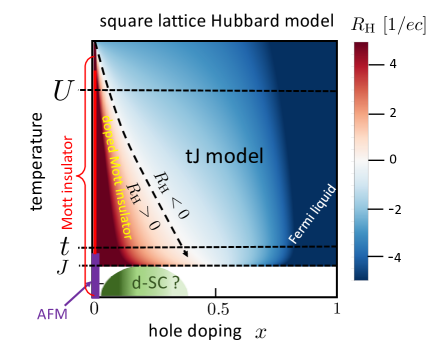
Figure 1: Hall coefficient $R_{\rm H}$ of the Hubbard Model with interaction $U$, and hopping $t$ on the square lattice (with unit lattice constant), as a function of hole doping per site $x$. We use the corresponding tJ-model at temperatures below the interaction scale $U$. In the low doping regime the Hall sign is reversed relative to the non-interacting model (see Fig. 2), and diverges. Antiferromagnetic (AFM) order sets in at $x=0$ below the magnetic energy scale $J$. A possible $d$-wave superconducting (d-SC) phase at low doping must inherit its charge carriers from the anomalous metallic state.

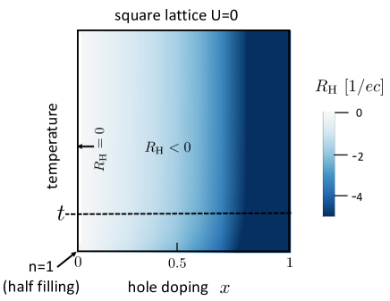
Figure 2: Hall coefficient of non-interacting electrons on a square lattice evaluated by Boltzmann theory, Eq. (1) for the a wavevector-independent scattering time. Note that $R_{\rm H}\!<\!0$ for $0\!<\!x\!<\!1$, and no divergence except at the empty band limit $x\to 1$.

A minimal model for doped Mott insulators is the strongly interacting ($U\!\gg\!t$) Hubbard model (HM) [10, 11]. At half filling (doping $x\!=\!0$) interactions open an insulating charge gap. At temperatures $T<U$ [12], its low frequency correlations are described by the tJ-model (tJM) [13, 12]. Variational studies of the square lattice HM and tJM, found $d$-wave superconductivity and charge ordering, depending on the details of the hopping terms [14, 15, 16]. Proxies for the Hall coefficient have been calculated [17, 18, 19, 20], but their error estimation remained a challenge. Quantum Monte Carlo (QMC) computations require an analytic continuation which is challenging in the DC limit [21].

A new thermodynamic formula for $R_{\rm H}$ includes a generally easy to compute ratio of susceptibilities $R_{\rm H}^{(0)}$ and a more complicated (but hopefully small) correction term $R^{\rm corr}_{\rm H}$ [22, 23, 24]. $R_{\rm H}^{(0)}$ was previously computed for the HM [25] by QMC. However for the HM, $R^{\rm corr}_{\rm H}$ increases with the interaction parameter $U/t$ and cannot be ignored, especially in the intermediate temperature (IT) regime defined by $t/2\leq T\leq U$.

This paper calculates the $R_{\rm H}^{(0)}$ for $U/t\gg 1$ by replacing the HM by the effective tJM. The doping dependence is obtained analytically by a high temperature expansion, and the lower temperatures in the IT regime by QMC sampling. Second order corrections of $R^{\rm corr}_{\rm H}$ for the tJM are calculated. They are found to be negligible relative to $R_{\rm H}^{(0)}$, and higher order corrections are estimated to be even smaller due to diminishing operator overlaps.

The temperature-doping Hall map is depicted in Fig. 1. It exhibits a substantial region of positive Hall coefficient, which diverges as $R_{\rm H}\!\propto\!1/x$ at temperatures lower than the $U$. The effects of the strong interactions are apparent by contrasting Fig. 1 with Fig. 2, which plots Boltzmann’s non-interacting result for the same square lattice with dispersion $\epsilon_{\bf k}=-2t\left(\cos(k_{x})+\cos(k_{y})\right)$ and isotropic scattering [26]:

$$R_{\rm H}^{\rm Boltz}={\int{d^{2}k\over(2\pi^{2})}\left(-{df\over d\epsilon}\right)\left({\partial\epsilon\over\partial k_{y}}\right)^{2}{\partial^{2}\epsilon\over(\partial k_{x})^{2}}\over 2\left(\int{d^{2}k\over(2\pi^{2})}\left(-{df\over d\epsilon}\right)\left({\partial\epsilon\over\partial k_{x}}\right)^{2}\right)^{2}},$$ (1)

where $f(\epsilon)$ is Fermi function. $R_{\rm H}^{\rm Boltz}$ yields a negative Hall coefficient at all hole dopings. Even with the addition of next nearest neighbor hopping, which is often included to fit the cuprates’ Fermi arcs, $R_{\rm H}^{\rm Boltz}$ would not be expected to diverge toward half filling.

At very high temperatures $T\gg U$, the effects of interactions in the HM are suppressed and $R_{\rm H}(x,T)\to R^{\rm Boltz}_{\rm H}(x,T)$. This regime may be accessed by cold atom simulations of the HM [27].

The Hall anomalies near the Mott phase are a consequence of the effective Gutzwiller projection (GP) in the IT regime [28]. The dynamical longitudinal conductivity is highly suppressed relative to the non-interacting limit. The sign reversal of $R_{\rm H}$ is due to interaction-driven density and spin operators which contribute to the commutators between GP currents and Hamiltonian. Thus, we learn that the currents are carried by a low density of spin-entangled positive vacancies moving in a paramagnetic environment. At lower temperatures, pairs of these projected hole carriers would form the expected [16] superconducting condensate, as proposed by Anderson [2].

The paper is organized as follows. The thermodynamic Hall coefficient formula, the HM and the tJM are formally introduced. The analytical high temperature expansion of the relevant susceptibilities for the tJM is presented. Numerical extension to lower temperatures by QMC simulations is displayed. The correction term is estimated, by evaluation of the second order contribution, and arguments for rapidly diminishing higher orders. Previous calculations of $R_{\rm H}$ using different methods are compared to our results. We conclude by summarizing the effects of strong Hubbard interactions on the charge carriers, and their implication on lower temperature transport in the expected superconducting flux flow regime [29].

II The Thermodynamic Hall Coefficient formula

The Hall coefficient $R_{\rm H}$, for a magnetic field ${\bf B}=B\hat{{\bf z}}$, is defined by elements of the conductivity tensor $\sigma_{\alpha\beta}$,

$$R_{\rm H}\equiv{d\sigma_{yx}\over dB}\sigma^{-2}_{xx}\Big{|}_{B\!=\!0}$$ (2)

which can be expressed by the thermodynamic formula $R_{\rm H}=R_{\rm H}^{(0)}+R^{\rm corr}_{\rm H}$ [23]. Both terms in $R_{\rm H}$ are composed of thermodynamic averages which are amenable to expansion in powers of inverse temperature $\beta$, and QMC without analytic continuation [21].

As derived in Refs. [22, 23], the first term $R_{\rm H}^{(0)}$ is a ratio of the current-magnetization-current (CMC) susceptibility and the conductivity sum rule (CSR) squared:

$$R_{\rm H}^{(0)}={\chi_{\rm cmc}\over\chi_{\rm csr}^{2}},$$

$$\chi_{\rm cmc}\!=\!-2{\mbox{Re}}\langle\big{[}P^{y},[M,j^{x}]\big{]}\rangle,~{}\chi_{\rm csr}\!=\!{\mbox{Im}}\langle\left[P^{x},j^{x}\right]\rangle,$$ (3)

where $\langle\cdot\rangle$ is the thermal expectation value. The operators $P^{\alpha},j^{\alpha}$ are the polarization and current in the $\alpha$ direction, and $M=-{\partial H\over\partial B}$ is the $z$-magnetization.

The correction term $R_{\rm H}^{\rm corr}$ is an infinite convergent sum which is defined in Appendix C. Since $R_{\rm H}^{\rm corr}$ is much harder to calculate, the formula is useful if it can be estimated to be negligibly small. For the tJM at high temperatures, we provide such an estimate in Section IV.1, by computing its leading orders as detailed in Appendix C.

III Hubbard and ${\rm tJ}$ Models

The square lattice HM (with units of $\hbar\!=\!1$) is,

$$H^{\rm HM}=-t\sum_{{\langle ij\rangle},s=\uparrow,\downarrow}(c^{\dagger}_{is}c^{{}^{\vphantom{\dagger}}}_{js}+c^{\dagger}_{js}c^{{}^{\vphantom{\dagger}}}_{is})+U\sum_{i}n_{i\uparrow}n_{i\downarrow},$$ (4)

where $c^{\dagger}_{is}$ creates an electron on site $i$ with spin $s$. ${\langle ij\rangle}$ are nearest neighbor bonds, and $n_{is}=c^{\dagger}_{is}c_{is}$. The Hall coefficient of the non-interacting model on the square lattice is negative (electron-like) without divergences for all $0\leq x<1$, as shown in Fig. 2.

For $U/t\gg 1$, the low energy subspace is defined by the GP operator ${\cal P}_{\rm GP}\!=\!\prod_{i}(1-n_{i\uparrow}n_{i\downarrow})$. The GP electron creation, hole density and spin operators are,

$${\tilde{c}}^{\dagger}_{is}\equiv c^{\dagger}_{is}(1-n_{i,-s}),\quad n^{h}_{i}\equiv 1-\sum_{s}{\tilde{c}}^{\dagger}_{is}{\tilde{c}}^{{}^{\vphantom{\dagger}}}_{is},$$

$$s^{\alpha}_{i}(1-n^{h}_{i})\equiv{1\over 2}\sum_{ss^{\prime}}{\tilde{c}}^{\dagger}_{is}\sigma^{\alpha}{\tilde{c}}^{{}^{\vphantom{\dagger}}}_{is^{\prime}}.$$ (5)

The electric polarization is defined by $P^{\alpha}=-e\sum_{i}x_{i}^{\alpha}n^{h}_{i}$, where $e$ is the negative electron charge, and ${\bf x}_{i}$ is the position of site $i$.

The GP hopping terms are,

$${K}^{\pm}_{ij}\equiv\sum_{s}{\tilde{c}}^{\dagger}_{is}{\tilde{c}}^{{}^{\vphantom{\dagger}}}_{js}\pm{\tilde{c}}^{\dagger}_{js}{\tilde{c}}^{{}^{\vphantom{\dagger}}}_{is},$$

$${\bf\Sigma}^{\pm}_{ij}\equiv\sum_{ss^{\prime}}{\tilde{c}}^{\dagger}_{is}\vec{\sigma}_{ss^{\prime}}{\tilde{c}}^{{}^{\vphantom{\dagger}}}_{js^{\prime}}\pm{\tilde{c}}^{\dagger}_{js}\vec{\sigma}_{ss^{\prime}}{\tilde{c}}^{{}^{\vphantom{\dagger}}}_{is^{\prime}}$$ (6)

where $K^{+}$ ($K^{-}$) describes the bond kinetic energy (current).

The adjacent-bond commutators for $a,a^{\prime}=\pm$ are

$$\!\!\!\!\!\![K^{a}_{12},K^{a^{\prime}}_{23}] = K^{-aa^{\prime}}_{13}\left({1+n^{h}_{2}\over 2}\right)+{\bf\Sigma}^{-aa^{\prime}}_{13}\cdot{\bf s}_{2}(1-n^{h}_{2}).$$ (7)

Note that these involve a hole density or spin operator on site $2$, which does not appear for a commutator of adjacent unprojected hopping operators . These extra operators are responsible for the sign reversal of $R_{\rm H}$ in the tJM at finite values of doping.

The tJM as derived from Eq. (4) [13, 12] can be expressed using Eq. (6),

$$H^{\rm tJM} = H^{t}+H^{J}+{\cal O}(t^{3}/U^{2})$$

$$H^{t} = -{t}\sum_{{\langle ij\rangle}}K^{+}_{ij},$$

$$H^{J} = -{J\over 4}\sum_{{\langle ij\rangle}{\langle jk\rangle}}\left(K^{+}_{ik}-2{\bf\Sigma}^{+}_{ik}\cdot{\bf s}_{j}\right)(1\!-\!n^{h}_{j}).$$ (8)

In the IT regime, $R_{\rm H}$ is largely determined by the hole hopping terms of $H^{t}$. $H^{J}$ scales with the superexchange energy $J=4t^{2}/U\!\ll\!t$, and includes spin interactions in its diagonal term, $i\!=\!k$, and (often neglected) next neighbor hopping terms $i\!\neq\!k$. The latter terms actually dominate to the Hall coefficient at very high temperatures $T\sim U$. For $H^{t}$, the current and magnetization are

$$j^{\alpha}_{ij}=-i{e\over\hbar a}{t}K^{-}_{ij;\alpha},$$

$$M={1\over 2c}\sum_{\langle ij\rangle}x_{i}j^{y}_{ij}-y_{i}j^{x}_{ij}.$$ (9)

Here, $ij;\alpha$, denotes a directed bond in the $\alpha$ direction, and $c$ is the speed of light. The additional contributions of $H^{J}$ to the current and magnetization are discussed in Section V.

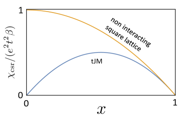
Figure 3: Doping dependent CSRs at intermediate temperatures. The suppression of the tJM CSR relative to the non-interacting square lattice CSR, affects a large region of doping. Vanishing of the tJM CSR at $x\to 0$ leads to the anomalous divergence of $R_{\rm H}$ toward the Mott phase, and the diverging resistivity slope.

IV Hall coefficient of the tJM

In the IT regime, $R_{\rm H}$ of the tJM (8) is dominated by $H^{t}$. For the CSR, the doping dependence of the two leading powers of inverse temperature $\beta$ were previously calculated by Jaklic [31] and Perepelitsky [32]. The calculation is reviewed in Appendix A, and yields

$$\!\!\!\!\chi^{t}_{\rm csr} = 2\beta e^{2}{t}^{2}x(1-x)$$ (10)

$$+ {\beta^{3}e^{2}{t}^{4}\over 6}x(1-x)(-9+2x+x^{2})+{\cal O}(\beta^{5}{t}^{6}).$$

As depicted in Fig. 3, the CSR (and therefore the whole dynamical longitudinal conductivity) of the tJM vanishes toward $x\to 0$, and is suppressed in a large region of doping. In contrast, the non-interacting CSR is maximized at half filling, as expected for a large Fermi surface.

The CMC of $H^{t}$ is evaluated up to order $(\beta{t})^{4}$ in Appendix A,

$$\chi^{t}_{\rm cmc} = -{\beta^{2}{t}^{4}e^{3}\over 2c}x(1-x)(-5+10x+3x^{2})$$ (11)

$$+ {\beta^{4}{t}^{6}e^{3}\over 16c}x(1-x)(45-136x+50x^{2}+48x^{3}-71x^{4})$$

$$~{}~{}~{}~{}~{}~{}~{}~{}~{}~{}~{}~{}~{}~{}~{}~{}~{}~{}~{}~{}~{}~{}~{}+{\cal O}(\beta^{6}{t}^{8}).$$

Thus, the zeroth order Hall coefficient in the IT regime is provided analytically as a function of doping and temperature:

$$R^{(0)}_{\rm H}={1\over ec}\left({-5+10x+3x^{2}\over 8x(1-x)}\right.+$$

$$~{}~{}~{}\left.(\beta{t})^{2}{-45-53x+145x^{2}+225x^{3}\over 192ex}\right).$$ (12)

The $\beta\to 0$ limit of Eq. (12) is depicted by the blue line in Fig. 4.

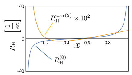
Figure 4: Second order Hall coefficient correction compared to the zeroth order Hall coefficient, as defined in Eq. (3). The ratio of magnitudes vanishes at $x\to 1$, and reaches $0.06$ at $x\to 0$.

IV.1 Estimation of $R^{\rm corr}_{\rm H}$ at high temperature

In Appendix C, the correction term is fully defined as a sum which contains conductivity recurrents and hypermagnetization matrix elements between higher order Krylov operators created by nested commutators $[[[H,H,\ldots,j^{\alpha}]]]$. We calculate the contribution of the first three terms,

$$R_{\rm H}^{{\rm corr}(2)}={1\over\chi_{\rm csr}}\left(\left({\Delta_{1}\over\Delta_{2}}\right)^{2}M_{2,2}^{\prime\prime}-\left({\Delta_{1}\over\Delta_{2}}\right)\left(M_{2,0}^{\prime\prime}+M_{0,2}^{\prime\prime}\right)\right)$$ (13)

where $\Delta_{1},\Delta_{2}$ are the first two recurrents of the longitudinal conductivity, which are evaluated analytically in Appendix A,

$$\Delta_{1}^{2}=t^{2}(3-2x-x^{2}),~{}~{}\Delta_{2}^{2}=t^{2}{24(1+x)\over 3+x}.$$ (14)

In Fig. 4, $R_{\rm H}^{{\rm corr}(2)}$ is plotted as a function of doping, and compared to the zeroth order term $R_{\rm H}^{(0)}$. The relative magnitude is qualitatively negligible and is maximized toward $x\to 0$ where

$$\lim_{x\to 0}\left|R_{\rm H}^{{\rm corr}(2)}/R^{(0)}_{\rm H}\right|\to 6\%.$$ (15)

Higher order correction terms $i,j\geq 2$ in Eq. 50 consist of products of ratios of consecutive recurrents $\Delta_{2j-1}\over\Delta_{2j}$ times the hypermagnetization matrix elements $M^{\prime\prime}_{2i,2j}$. These terms are expected to be strongly suppressed relative to the low order terms due to the following argument: While generically the ratios of $\Delta_{n}/\Delta_{n+1}$ do not asymptotically decay rapidly with $n$ [33], $M^{\prime\prime}_{n,m}$ at high temperature are expected to diminish rapidly with $n,m$, since they involve traces over two clusters of operators which are created by nested commutators ${\cal L}^{m}j^{x}=[H,[H,\ldots,j^{x}]]$ and ${\cal L}^{n}j^{y}=[H,[H,\ldots,j^{y}]]$. The number of clusters in each of the normalized Krylov states increases faster than exponentially. Since the clusters created from the $x$ and $y$ currents occupy partially overlapping areas on the lattice, the fraction of operators which precisely match the sites of $\tilde{c}_{i},\tilde{c}_{i}^{\dagger},s^{\alpha}_{i}$ decreases rapidly with the order of the normalized Krylov states. This effect is proven already by the relative small size of $R_{\rm H}^{{\rm corr}(2)}/R_{\rm H}^{(0)}$, and we expect the relative contributions of the rest of the corrections to be even smaller.

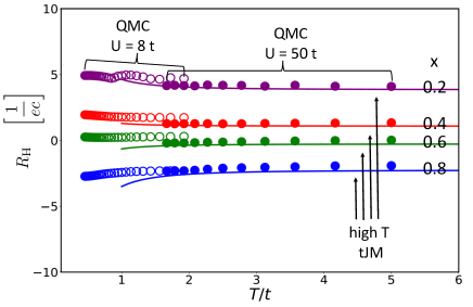
Figure 5: Hall coefficient $R_{\rm H}^{(0)}$ in the intermediate temperature regime $J<T<U$. Lines depict the high temperature expansion results, Eq. (12). Solid and open circles are QMC results using HM weights, for two values of $U/t$. The QMC results are plotted in the regions of negligible fermion sign error (see Appendix IV.2). We note that the high temperature expansion agrees with the QMC data down to $T\simeq 2t$, and that $R_{\rm H}$ shows quite weak temperature dependence down to $T\simeq 0.5t$.

IV.2 QMC extension to lower temperatures

The QMC extends the calculation of $R^{(0)}_{\rm H}$ of the tJM to larger values of $\beta$.

A determinantal QMC calculation for lattice fermions with discrete auxiliary fields was implemented using the ALF package [34]. We used HM weights for $U/t=8,16,50$. The typical system size was chosen to be $8\!\times\!8$, with little size dependence, which was tested up to size $12\!\times\!12$, indicating short correlation length in the studied temperature regime. The imaginary time step was chosen to render the Trotter errors to be insignificant. The number of Monte Carlo sweeps was generally $\sim 10^{5}$. The statistics was quite well-behaved, and “Jackknife resampling” (a method used for error estimation), revealed sufficiently small error bars. The average sign in the QMC sampling is defined as

$$\langle S\rangle=\langle\mbox{\rm sgn}({\rm det})\rangle.$$ (16)

In Appendix E, we report the value of $\langle S\rangle$ as a function of interaction strength $U/t$, doping and temperature. We show that quite generally, $\langle S\rangle$ approaches unity at higher temperatures where the Fermionic negative weights introduce negligible effects on QMC configuration averaging.

The CMC and CSR susceptibilities of Eq. (3) were computed by sampling products of Green’s functions using Wick’s theorem over QMC equilibrium configurations of the auxiliary fields. In Fig. 5 the QMC results are depicted by circles of larger diameter than the numerical error bars. The displayed data is restricted to the regime of $\langle S\rangle\geq 0.8$, which for $U=8t$ and all doping range is satisfied at $T\geq t/2\approx J$. We note that the data exhibits a weaker temperature dependence than expected by extrapolating the analytic high temperature results.

V $R_{\rm H}$ at very high temperatures

At very high temperatures $T>U$, $R_{\rm H}$ for HM is obtained by a high temperature expansion in powers of $\beta U\ll 1$. The commutators between unprojected magnetization and currents do not involve interaction terms, and are bilinear in fermion operators. The leading orders in the high temperature expansion are given by traces over these operators,

$$\chi^{U}_{\rm csr}\sim\beta e^{2}t^{2}n(2-n),\quad\chi^{U}_{\rm cmc}\sim\beta^{2}{e^{3}\over c}t^{4}n(2-n)(1-n)$$

$$R^{U}_{\rm H}={2(1-n)\over n(2-n)ec}+{\cal O}(\beta U)^{2},$$ (17)

where $n=1-x$ is the electron density. Thus, the leading order in $R^{U}_{\rm H}$ recovers the high temperature expansion of the non-interacting square lattice coefficient which is depicted in Fig. 2.

Interestingly, this effect is qualitatively implemented by the addition of the next neighbor hopping term $H^{J}$ of order $J$ in the tJM. As a hopping term, $H^{J}$ in Eq. (8) contributes terms of order $J\ll t$ to the current and magnetization operators,

$${j^{\prime}}^{\alpha}_{ijk}=-ieJ(1-n^{h}_{j})\left(K^{-}_{ik;\alpha}-2{\bf\Sigma}^{-}_{ik;\alpha}\cdot{\bf s}_{j}\right)$$

$$M^{\prime}={1\over 2c}\sum_{{\langle ijk\rangle}}(x_{i}{j^{\prime}}^{y}_{ijk}-y_{i}{j^{\prime}}^{x}_{ijk}).$$ (18)

Since $H^{J}$ connects sites across the plaquette diagonals, its high temperature expansion yields a power of $\beta J$, which is one power lower than the leading power of $\chi^{t}_{\rm cmc}$, (see Appendix B). Thus,

$$\chi^{tJ}_{\rm cmc}=\chi^{t}_{\rm cmc}+{\beta Je^{3}\over 2}x(1-x)(1+2x-3x^{2})(1+{\cal O}(t/U)).$$ (19)

Combining the Hall coefficients of Eq. (12) with the contribution of $H^{J}$ to the second order in $\beta{t}$, and neglecting the correction term and terms of order $t/U$ yields

$$R^{tJ}_{\rm H}=R^{t}_{\rm H}+{1\over ec}{4\over\beta U}{(1+2x-3x^{2})\over 8ex(1-x)}.$$ (20)

The additional term is opposite in sign to $R_{\rm H}^{t}$. For $\beta U<4$ (beyond the validity of the tJM), $R_{\rm H}$ is expected to become negative as depicted in Fig. 1.

VI Resistivity slope

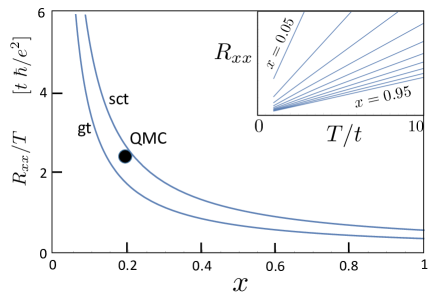
Figure 6: High temperature resistivity slopes of $H^{t}$ as a function of doping $x$. SCT and GT denote two different continued fraction extrapolation schemes (see text). Inset depicts $R_{xx}(T)$ for the GT. The solid circle marks the QMC result for the $U\!=\!8t$ HM, reported in Fig. S3 of Ref. [35].

The continued fraction expression for the longitudinal conductivity [36, 37] is given by

$$\sigma_{xx}(\omega)=\beta\chi_{\rm csr}{\mbox{Im}}{1\over-\Delta_{1}^{2}G_{2}(-i\varepsilon)}$$ (21)

where $\Delta_{1},\Delta_{2}$ and $G_{2}$ are the first two conductivity recurrents, and the estimated second order termination function respectively. $G_{2}$ is estimated by two extrapolation schemes. First, we use the semicircle termination (SCT) where all higher order recurrents are assumed to be equal to $\Delta_{2}$,

$$\Delta^{\rm sct}_{n}=\Delta_{2},\quad n=2,3\ldots\infty.$$ (22)

This yields an algebraic equation for $G_{2}$,

$$G^{\rm sct}_{2}(-i\varepsilon) = {1\over-i\varepsilon-\Delta_{2}^{2}G_{2}(-i\varepsilon)},$$

$${\mbox{Im}}G^{\rm sct}_{2} = -{1\over\Delta_{2}},$$

$$\sigma^{\rm sct}_{xx} = \beta\chi_{\rm csr}{\Delta_{2}\over\Delta_{1}^{2}},$$

$$R^{\rm sct}_{xx} = T{\Delta_{1}^{2}\over\chi_{\rm csr}\Delta_{2}}={T\over t}{(3+x)^{3\over 2}\over 4\sqrt{6}x\sqrt{1+x}}.$$ (23)

Second, we use the Gaussian termination (GT), which assumes that the recurrents $\Delta_{n\geq 2}$ scale as $\sqrt{n}$,

$$(\Delta^{\rm gt}_{n})^{2}={1\over 2}n\Delta^{2}_{2},\quad n=2,3,\ldots\infty.$$ (24)

This extrapolation yields,

$${\mbox{Im}}G^{\rm gt}_{2}(0) = -{2\over\sqrt{\pi}\Delta_{2}},$$

$$\sigma^{\rm gt}_{xx} = \beta{\sqrt{\pi}\over 2}\chi_{\rm csr}{\Delta_{2}\over\Delta_{1}^{2}}.$$ (25)

We note that the two different extrapolations yield similar results for the DC resistivity $R_{xx}=\sigma_{xx}^{-1}$:

$$R^{\rm gt}_{xx}={2\over\sqrt{\pi}}R^{\rm sct}_{xx}.$$ (26)

In Fig. 6, the resistivity slopes of $H^{t}$ are plotted using the SCT and GT extrapolations. We note that the slopes diverge toward the Mott limit, as expected by the suppression of the CSR depicted in Fig. 3. Interestingly, the resistivity is finite at high temperatures even in the dilute electron density limit $x\to 1$. We note a quantitative agreement of the slope with the calculation of HM recurrents in Ref. [35].

VII Discussion

A relevant precursor to our work includes the calculation of the high frequency limit of the Hall coefficient of the tJM by Shastry, Shraiman and Singh [38]. It is interesting (but far from obvious) that they have found a qualitatively similar doping dependence to the zero frequency Hall coefficient calculated here. We also note that sign reversals and Hall coefficient increase towards the Mott limit have been obtained in some parameter ranges of the HM using dynamical mean field theory [18, 19, 20].

The formula for $R_{\rm H}^{(0)}(x,T)$ given in Eq. (3) was computed by QMC for the HM [25, 19]. A Hall coefficient sign reversal and increase toward the Mott phase was detected albeit with a much reduced magnitude relative to the tJM calculation. This difference is attributed to the use of the HM for large $U/t$ instead of the lower energy effective tJM. The CSR of the HM includes dynamical conductivity contributions above the Hubbard gap. Hence, the denominator of $R_{\rm H}$ does not vanish at zero doping, and it does for the tJM. $R_{\rm H}$ can be calculated in principle using either HM or tJM. However, since $R_{\rm H}^{\rm corr}$ depends on $[H,j^{x}]$, the HM whose current-Hamiltonian commutator scales with the interaction strength $U$, produces a larger correction than the tJM.

Our results lead to the following conclusions:

(i) Strong interactions which open a Mott gap at zero doping, also affect the sign and density of charge carriers in a sizeable portion of the Hall map as depicted in Fig. (1).

(ii) $R_{\rm H}$ and $R_{xx}/T$ increase as $x\to 0$ due to the suppression of the CSR toward the Mott insulator.

(iii) The spin-charge correlated commutators of the GP currents of Eq. (7), are the source of the Hall sign reversal at finite doping.

At lower temperatures than discussed in this work, one still expects the strong interactions to have implications on the charge transport. If, as numerically predicted [14, 15, 16], $d$-wave superconductivity emerges at low doping of the tJM, its condensate should be described by a low density of GP hole pairs, rather than the Cooper pairs on a narrow shell on the putative band-theory predicted Fermi surface.

The experimental manifestation of the positive constituent charges in cuprates is found in Hall conductivity above and below the superconducting temperature. Bardeen and Stephen theory predicts the same Hall sign in the flux flow regime as in the normal phase [39]. At lower temperatures, the Hall conductivity acquires an additional negative contribution from the vortex charge [29], which depends on the derivative of the superfluid stiffness $\rho_{s}$ with respect to electron density $n_{e}$. The negative sign of $d\rho_{s}/dn$ at low doping [40] is consistent with a condensate of positively charged hole pairs.

Acknowledgements – We thank Omer Yair who worked on a predecessor of this project, and Netanel Lindner, Edward Perepelitsky, Sriram Shastry, and Efrat Shimshoni for useful discussions. A.S. and S.B thank Fakher Assaad and Johannes Hoffmann for their help in application of the ALF numerical packages. We acknowledge the Israel Science Foundation Grant No. 2021367. This work was performed in part at the Aspen Center for Physics, supported by National Science Foundation grant PHY-1607611, and at Kavli Institute for Theoretical Physics, supported by Grant No. NSF PHY-1748958.

Appendix A High temperature expansion of the susceptibilities

In the grand cannonical ensemble, the mean density of holes for the tJM can be imposed at infinite temperature by a product density matrix $\rho_{0}(\delta)$, with a fugacity parameter $\delta$:

$$\rho_{0}(\delta)=\prod_{i}\left(\delta|h_{i}\rangle\langle h_{i}|+\sum_{s=\uparrow,\downarrow}{1-\delta\over 2}|s_{i}\rangle\langle s_{i}|\right),$$ (27)

where $|h_{i}\rangle$ is a hole at size $i$, and the average hole density at infinite temperature is

$$x(0)=\langle n^{h}_{i}\rangle_{\beta=0}\equiv\delta.$$ (28)

Expectation values are,

$${\mbox{Tr}}\rho_{0}s_{i}^{\alpha}(1\!-\!n^{h}_{i}) = 0,$$

$${\mbox{Tr}}\rho_{0}{\bf s}^{2}_{i}(1\!-\!n^{h}_{i}) = {3\over 4}(1-\delta).$$ (29)

Using the relation,

$$K^{s,a}_{12}K^{s,a}_{21}=n^{h}_{1}+n^{h}_{2}-2n^{h}_{1}n^{h}_{2},$$ (30)

we obtain some useful traces on two-site operators:

$${\mbox{Tr}}\rho_{0}(K_{12}^{+})^{2} = -{\mbox{Tr}}(K_{12}^{-})^{2}=2\delta(1-\delta)$$

$${\mbox{Tr}}\rho_{0}\left(\Sigma^{+}_{12,\alpha}\right)^{2} = -{\mbox{Tr}}\left(\Sigma^{-}_{12,\alpha}\right)^{2}=2\delta(1-\delta)$$

$${\mbox{Tr}}\rho_{0}s^{\alpha}_{i}s^{\beta}_{j} = \delta_{ij}\delta_{\alpha\beta}{1\over 4}.$$ (31)

At finite temperatures, we expand the average hole density $x(\delta)$ to second order in $\beta$,

$$x = {{\mbox{Tr}}\rho_{0}(\delta)e^{-\beta H}n^{h}_{i}\over{\mbox{Tr}}\rho_{0}(\delta_{0})e^{-\beta H}}=\delta+{\beta^{2}\over 2}{\mbox{Tr}}\rho_{0}(\delta)H^{2}(n^{h}_{i}-\delta)$$ (32)

$$= \delta+2\beta^{2}(1-2\delta)\delta(1-\delta)+{\cal O}(\beta^{4}).$$

Eq. (32) allows us to evaluate the density dependence of a $\delta$-dependent susceptibility by

$$\chi(\delta,\beta)=\chi(x-2\beta^{2}(1-2\delta)\delta(1-\delta),\beta).$$ (33)

A.1 CSR

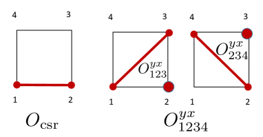
Figure 7: Operators which are averaged over in the CSR and CMC. Line denotes a bond operators $K^{+}$ or ${\bf\Sigma}_{\alpha}^{+s}$, and the circle denotes a site operator ${1+n^{h}\over 2}$ or $s^{\alpha}(1-n^{h})$, respectively.

The first two leading orders in $(\beta t)$ of the CSR are defined as,

$$\bar{\chi}_{\rm csr}=e^{2}(\beta{t})\bar{\chi}^{(1)}_{\rm csr}+e^{2}(\beta{t})^{3}\bar{\chi}^{(3)}_{\rm csr}+\ldots.$$ (34)

where, using (30),

$$\bar{\chi}_{\rm csr}^{(1)}={\mbox{Tr}}\rho_{0}(K^{+}s_{12})^{2}=2x(1-x).$$ (35)

The order $\beta^{3}$ CSR is obtained by expanding the Boltzmann weight and the partition function,

$$\bar{\chi}_{\rm csr}^{(3)}(\delta)={1\over 6}\Big{(}\overbrace{-{\mbox{Tr}}_{c}\rho_{0}((H/t)^{3}K^{+}s_{12})}^{A}-21\overbrace{\left({\mbox{Tr}}\rho_{0}(K_{12}^{+}s)^{2}\right)^{2}}^{B}\Big{)},$$ (36)

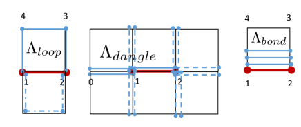
Figure 8: Graphs of operators which contribute to the term $A$ in Eq. (36).

where $c({12})$ includes all the $H$-bonds emanating from sites 1,2, as depicted in Fig.8. The traces yield,

$$A=\delta(1-\delta)\left(15-10\delta+13\delta^{2}\right),$$

$$B=84\delta^{2}(1-\delta)^{2},$$

$$\bar{\chi}_{\rm csr}^{(3)}(\delta)={1\over 6}\delta(1-\delta)\left(15-94\delta+97\delta^{2}\right).$$ (37)

Using Eq. (33) to transform $\chi_{\rm csr}(\delta)$ to $\chi_{\rm csr}(x)$ yields,

$$\chi_{\rm csr}^{(3)}(x) = \bar{\chi}_{\rm csr}^{(3)}(x)-{\partial\bar{\chi}_{\rm csr}^{(1)}\over\partial x}2(1-2x)x(1-x)$$ (38)

$$= {1\over 6}x(1-x)(-9+2x+x^{2}).$$

This recovers Eq. (10), which was previously published in Ref.[32].

The CMC is given by averaging the plaquette operator, shown in Fig. 7.

$$\chi_{\rm cmc} = -2e^{3}{t}^{3}\langle O^{yx}_{123}\rangle$$

$$= 2e^{3}{t}^{3}\langle\left(K^{+}s_{13}{1+n^{h}_{2}\over 2}+{\bf\Sigma}^{+}s_{13}s^{\alpha}_{2}(1-n^{h}_{2})\right)\rangle,$$

where we have used using C4 symmetry to equate four identical contributions to the expectation value. The leading order $\chi^{(2)}_{\rm cmc}$ requires tracing $O^{yx}_{123}$ times two Hamiltonian bonds in a connected cluster inside a plaquette. The calculation yields

$$\chi^{(2)}_{\rm cmc} = -{\mbox{Tr}}\rho_{0}(\beta H)^{2}O^{yx}_{123}$$ (40)

$$= {\beta^{2}\over 2}x(1-x)(-5+10x+3x^{2}).$$

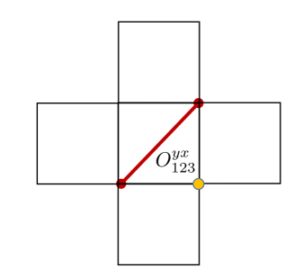
Figure 9: Minimal connected cluster for the calculation of $\chi^{(4)}_{\rm cmc}$, which must include 4 powers of $H$ whose bonds connect to the sites of $O^{yx}_{123}$ and contribute to a non vanishing trace.

The order $\beta^{4}$ is given by

$$\chi_{\rm cmc}^{(4)}(\delta)=-{1\over 12}{\mbox{Tr}}_{c}\rho_{0}(\beta H/t)^{4}O^{yx}_{123})$$

$$~{}~{}~{}~{}~{}~{}-8\delta^{2}(1-\delta)^{2}(-5+10\delta+3\delta^{2}).$$ (41)

The first term in (41) which is calculated on the lattice shown in Fig. 9, is computed by symbolic multiplication.

$${\mbox{Tr}}_{c}\rho_{0}((H/t)^{4}O^{yx}_{123})={1\over 4}\delta(1-\delta)$$

$$~{}~{}~{}~{}~{}~{}~{}~{}\times\left(213\delta^{4}+1104\delta^{3}-2022\delta^{2}+408\delta+105\right).$$

This results in,

$$\chi_{\rm cmc}^{(4)}(\delta)={1\over 16}\delta(1-\delta)(-35+504\delta-1246\delta^{2}+528\delta^{3}+313\delta^{4}).$$ (43)

Transforming the expression using Eq. (33), yields

$$\chi_{\rm cmc}^{(4)}(x) = \lim_{\delta\to x}\{\chi_{\rm cmc}^{(4)}(\delta)-(\partial_{\delta}\chi^{(2)}_{\rm cmc})2(1-2\delta)\delta(1-\delta)\}$$

$$= {x(1-x)\over 16}(45-136x+50x^{2}+48x^{3}-71x^{4}),$$

which arrives at Eq. (11).

Appendix B Leading order effect of $H^{J}$

The correlated hopping term in $H^{J}$ of Eq. (8) closes a loop of three bonds on the square lattice, which produces terms of order $(\beta J)$ in the CMC. Collecting the leading orders in $(\beta J)$ from $H^{J}$, the currents and magnetization yields

$$\chi_{\rm cmc}^{J}=2e^{3}\beta Jt^{2}\beta(C_{1}+C_{2}),$$ (45)

where

$$C_{1}\equiv{\mbox{Tr}}\rho(H^{J}/J)O^{yx}_{123}=-{1\over 4}\delta(1-\delta)^{3},$$ (46)

and

$$C_{2} \equiv {\mbox{Tr}}\rho_{0}K_{14}^{+}\left[-n^{h}_{4},[j^{J}_{234}/J,j^{x}_{12}]\right]$$ (47)

$$+{\mbox{Tr}}\rho_{0}K_{14}^{+}\left[-n^{h}_{4},[-j^{x}_{43},j^{J}_{123}/J]\right],$$

$$= 2\times{1\over t}{\mbox{Tr}}\rho_{0}(K_{14}^{+}s)^{2}{1+n^{h}_{2}\over 2}(1-n^{h}_{3})$$

$$= {1\over 2}x(1-x)(1-x^{2}).$$

Thus,

$$\chi_{\rm cmc}=\chi^{t}_{\rm cmc}+{\beta Je^{3}t^{3}\over 2}x(1-x)(1+2x-3x^{2}),$$ (48)

which yields expression (20). The order $J=4t^{2}/U$ becomes as large as $\chi_{\rm cmc}^{t}$ at around $T\geq U$, which is where the renormalization of the HM onto the tJM ceases to be valid.

Appendix C Second order corrections of the Hall coefficient formula

At high temperatures, the scalar product between operators is given by

$$(A|B)=\beta{\mbox{Tr}}A^{\dagger}B+{\beta^{2}\over 2}{\mbox{Tr}}\{H,A^{\dagger}\}B+{\cal O}(\beta^{3}).$$ (49)

The Hall coefficient correction [23],

$$R_{\rm H}^{\rm corr} = {1\over\chi_{\rm csr}}\sum_{i,j=0}^{\infty}R_{i}R_{j}(1-\delta_{i,0}\delta_{j,0})M^{\prime\prime}_{2i,2j}$$

$$M^{\prime\prime}_{2i,2j} = {\mbox{Im}}\left(\langle(2i)_{y}|{\cal M}|(2j)_{x}\rangle]-\langle(2i)_{x}|{\cal M}|(2j)_{y}\rangle]\right),$$

$$R_{i>1} = \prod_{r=1}^{i}\left(-{\Delta_{2r-1}\over\Delta_{2r}}\right)\quad R_{0}=1.$$ (50)

The recurrents are defined as $\Delta_{0}=0$,

$$\Delta_{n}\equiv\langle(n)_{x}|{\cal L}(n+1)_{x}\rangle,n\in\mathbb{Z},$$ (51)

which can be obtained from the lower order conductivity moments $\mu_{2k}$ of orders $k\in\mathbb{Z}$, where

$$\mu_{2k}=(j^{x}|{\cal L}^{2k}|j^{x})=-{\mbox{Im}}\langle[j^{x},{\cal L}^{2k-1}j^{x}]\rangle,$$ (52)

where the Liouvillian hyperoperator is defined as ${\cal L}O=[H,O]$, $j^{\alpha}=i\left[H,P^{\alpha}\right]$ and $\mu_{0}=\chi_{\rm csr}$.

The magnetization hyperoperator is ${\cal M}O=[M,O]$. The orthonormal Krylov states $|(n)_{\alpha}\rangle$, which define the matrix elements $M_{2i,2j}^{\prime\prime}$ are a set of operators (hyperstates) created by applying ${\cal L}^{n}$ to the current ${\cal L}^{n}|j^{\alpha}\rangle=\left[H,\left[H,...\left[H,j^{\alpha}\right]\right]\right]$ [23], and orthonormalizing the result with respect to the lower order states. The Krylov basis is thus constructed as,

$$|(0)_{\alpha}\rangle={|j^{\alpha})\over\sqrt{\chi_{\rm csr}}},$$ (53)

and

$$|(n+1)_{\alpha}\rangle={{\cal L}|(n)_{\alpha}\rangle-\Delta_{n}|(n-1)_{\alpha}\rangle\over(\langle(n)_{\alpha}|{\cal L}^{2}|(n)_{\alpha}\rangle-\Delta_{n}^{2})^{1\over 2}},\quad n\geq 1.$$ (54)

The second order correction terms of Eq. (13) include two recurrents $\Delta_{1},\Delta_{2}$ and three the hypermagnetization matrix elements $M_{0,2}^{\prime\prime},M_{2,0}^{\prime\prime},M_{2,2}^{\prime\prime}$.

C.1 $\Delta_{1}$

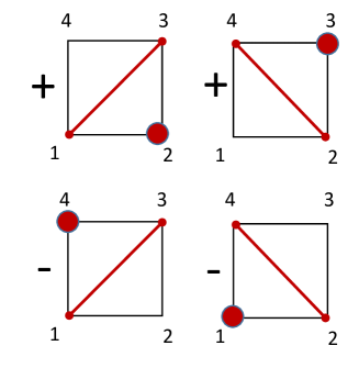
Figure 10: Operators of first unnormalized Krylov hyperstate $|(1)_{x})=[H^{t},j^{x}]$. Solid line and circle represent the product of bond and site operators $K_{ij}^{+}s$, $(1+n_{k}^{h})/2$ respectively, or $\Sigma^{+}s_{\alpha,ij}$ and ${\bf s}_{k}^{\alpha}(1-n_{k}^{h})$.

The first Krylov state ${\cal L}j^{x}$ and ${\cal L}j^{y}$ is described by the diagrams of Fig. 10,

$${\cal L}j^{x} = \sum_{i}C_{13}^{x}\left(K^{+}s_{13}{(n^{h}_{2}-n^{h}_{4})\over 2}+\Sigma_{13,+s}^{\alpha}(s^{\alpha}_{2}-s^{\alpha}_{4})\right)$$

$$+C_{42}^{x}\left(K^{+}s_{42}{(n^{h}_{3}-n^{h}_{1})\over 2}+\Sigma_{42,s}^{\alpha}(s^{\alpha}_{3}-s^{\alpha}_{1})\right)$$

$${\cal L}j^{y} = \sum_{i}C_{13}^{y}\left(K^{+}s_{13}{(n^{h}_{2}-n^{h}_{4})\over 2}+\Sigma_{13,s}^{\alpha}(s^{\alpha}_{2}-s^{\alpha}_{4})\right)$$

$$+C_{42}^{y}\left(K^{+}s_{42}{(n^{h}_{3}-n^{h}_{1})\over 2}+\Sigma_{42,s}^{\alpha}(s^{\alpha}_{3}-s^{\alpha}_{1})\right),$$

where the coefficients

$$(C_{13}^{x},C_{42}^{x})=(1,1),\quad(C_{13}^{y},C_{42}^{y})=(-1,1),$$ (56)

depend on the symmetries of $j^{x},j^{y}$ respectively.

The first recurrent is defined by the norm of the operator ${\cal L}j^{x}/\chi_{\rm csr}^{1\over 2}$:

$$\Delta_{1}^{2} = {\beta\over\chi_{\rm csr}}{\mbox{Tr}}j^{x}{\cal L}^{2}j^{x}$$

$$={t^{2}\over\chi_{\rm csr}}2{\mbox{Tr}}\rho_{x}\left(K_{13,a}K_{31,a}{(n^{h}_{2}-n^{h}_{4})^{2}\over 4}\right.$$

$$+\left.2\times 3\Sigma^{z}_{13,a}\Sigma^{z}_{31,a}(s^{z}_{2})^{2}\right)$$

$$= {\beta\over\chi_{\rm csr}}t^{2}2x(1-x)\left(x(1-x)+3(1-x)\right)=3-2x-x^{2},$$

which is given in the main text, Eq. (14). Note that $\Delta_{1}^{2}$ is positive at all dopings, and vanishes at $x\to 1$ due to absence of scattering in the empty band. Notice that near the Mott phase, $x\to 0$, $\Delta_{1}$ is dominated by the $({\bf\Sigma}\cdot{\bf s})^{2}$ term, representing scattering of holes from spins.

C.2 $\Delta_{2}$

The second recurrent is given by the equation,

$$\Delta_{2}^{2}={\mu_{4}\over\Delta_{1}^{2}\chi_{\rm csr}}-\Delta_{1}^{2}={\mu^{\prime}_{4}\over\Delta_{1}^{2}\chi_{\rm csr}},$$ (58)

where the fourth moment is

$$\mu_{4}=\beta{\mbox{Tr}}\rho_{x}j^{x}{\cal L}^{4}j^{x},$$ (59)

which contains the traces of the squares all non-returning (${\cal L}^{2}j^{x}\propto j^{x}$) ) operators in ${\cal L}^{2}j^{x}$.

The classes of operators are listed in Fig. 11. The arrows mark the charge and spin bond operators and the circles mark density and spin site operators. In the numbers $a(b)$, $a$ is the lattice symmetry factor, and $(b)$ is the number of identical operators created by $(1-|0_{x}\rangle\langle 0_{x}|){\cal L}^{2}\sum_{i}j^{x}_{i}$.

The operators are,

$$A_{ij;kl} = K_{ij;a}\left({1\over 4}(1+n_{k}^{h})(1+n_{l}^{h})+s^{\alpha}_{k}s^{\alpha}_{l}\right)$$

$$+\Sigma^{\alpha}_{ij;a}\left(s^{\alpha}_{k}{1+n_{l}^{h}\over 2}+s^{\alpha}_{l}{1+n_{k}^{h}\over 2}\right)$$

$$+\epsilon_{\alpha\beta\gamma}\Sigma_{ij,s}^{\alpha}s_{k}^{\beta}s_{l}^{\gamma}$$

$$D_{ij;kl} = {1\over 2}K_{ij;s}\vec{K}_{jl}+{1\over 2}\Sigma^{\alpha}_{ij;s}\vec{\Sigma}^{\alpha}_{jl}.$$ (60)

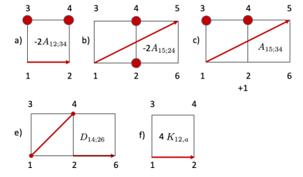
Figure 11: Classes of operators of ${\cal L}^{2}j^{x}$, $K$, $A$ and $D$ are defined in Eqs. (6) and (60).

Thus,

$${\mu_{4}\over\beta t^{6}} = \overbrace{{\mbox{Tr}}(\underbrace{4}_{degen.}K_{12,a}^{\dagger})(4K_{12,a})}^{\mbox{bare curr}^{2}}$$

$$-2{\mbox{Tr}}(4K_{12,a}^{\dagger})(2A_{12;34}+2A_{12;78})$$

$$+{\mbox{Tr}}(2A_{12;34}+2A_{12;78})^{\dagger}(2A_{12;34}+2A_{12;78})$$

$$+\underbrace{8}_{rotations}{\mbox{Tr}}\left(A^{\dagger}_{15;34}A_{15;34}+A_{15;24}(2A_{15;24})\right.$$

$$\left.-A^{\dagger}_{15;34}(2A_{15;24})+A^{\dagger}_{15;34}A_{15;26}\right)+8{\mbox{Tr}}D^{\dagger}D,$$

which yields

$$\Delta_{2}^{2}={\mu_{4}\over\Delta_{1}^{2}\chi_{\rm csr}}-\Delta_{1}^{2}=t^{2}{24(1+x)\over 3+x}\to_{x\to 0}8\quad\to_{x\to 1}12,$$ (62)

as depicted in Fig. 12 and shown Eq. (14).

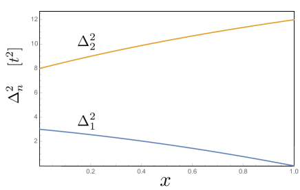
Figure 12: The doping dependence of the first two recurrents of $H^{t}$ at high temperature.

Appendix D Numerical calculation of recurrents and hypermagnetization matrix elements

The moments $\mu_{2},\mu_{4}$ which yield the recurrents $\Delta_{1},\Delta_{2}$ as well as the three hypermagnetization corrections $M^{\prime\prime}_{02},M^{\prime\prime}_{20},M^{\prime\prime}_{22}$ were evaluated numerically. They are written as expectation values of connected clusters of site operators. The clusters are formed by commuting bond operators of the Hamiltonian or magnetization with the root current operator $j_{i}^{\alpha}$ on a single bond at site $i$. The result of ${\cal L}^{n}j^{\alpha}_{i}$ is a large sum of multi-site products of operators $O_{i_{1}}({{\bf r}_{1}})\cdot O_{i_{2}}({\bf r}_{2})\cdot...\cdot O_{i_{N}}({\bf r}_{N})$, which is viewed as a product “hyperstate” in operator space, with a complex amplitude that is stored separately. Each application of the Liouvillian or the hypermagnetization can create a new hyperstate by multiplying the individual site operators site-by-site using the multiplication Table 1. One must keep track of the order of the fermionic operators $\tilde{c}_{i},\tilde{c}_{j}^{\dagger}$, and the negative signs produced when collecting contributions to the same product state from different multiplication paths.

	$\tilde{c}^{\dagger}_{\uparrow}$	$\tilde{c}^{\dagger}_{\downarrow}$	$\tilde{c}_{\uparrow}$	$\tilde{c}_{\downarrow}$	$n_{\uparrow}$	$n_{\downarrow}$	$\tilde{s}^{+}$	$\tilde{s}^{-}$
$\tilde{c}^{\dagger}_{\uparrow}$	0	0	$n_{\uparrow}$	$\tilde{s}^{+}$	0	0	0	0
$\tilde{c}^{\dagger}_{\downarrow}$	0	0	$\tilde{s}^{-}$	$n_{\downarrow}$	0	0	0	0
$\tilde{c}_{\uparrow}$	$n_{h}$	0	0	0	$\tilde{c}_{\uparrow}$	0	$\tilde{c}_{\downarrow}$	0
$\tilde{c}_{\downarrow}$	0	$n_{h}$	0	0	0	$\tilde{c}_{\downarrow}$	0	$\tilde{c}_{\uparrow}$
$n_{\uparrow}$	$\tilde{c}^{\dagger}_{\uparrow}$	0	0	0	$n_{\uparrow}$	0	$\tilde{s}^{+}$	0
$n_{\downarrow}$	0	$\tilde{c}^{\dagger}_{\downarrow}$	0	0	0	$n_{\downarrow}$	0	$\tilde{s}^{-}$
$\tilde{s}^{+}$	0	$\tilde{c}^{\dagger}_{\uparrow}$	0	0	0	$\tilde{s}^{+}$	0	$n_{\uparrow}$
$\tilde{s}^{-}$	$\tilde{c}^{\dagger}_{\downarrow}$	0	0	0	$\tilde{s}^{-}$	0	$n_{\downarrow}$	0

Table 1: Multiplication table of GP operators in the tJM. The entry $O_{i,j}=O_{i}\cdot O_{j}$, where $i$ and $j$ are row and column respectively.

where,

$$\tilde{s}^{\alpha}=s^{\alpha}(1-n^{h}),\quad n_{\uparrow,\downarrow}=(1-n^{h})\left({1\over 2}\pm s^{z}\right).$$ (63)

For traces however, most operators vanish unless they contain only constants and factors of density $n_{\gamma}$, (see Eqs. (27-31).

Appendix E QMC sign errors

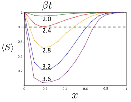
Figure 13: QMC fermion sign average for the HM as a function of doping for $U=8t$, and for a set of inverse temperatures $\beta$.

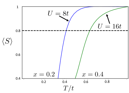
Figure 14: QMC fermion sign average for the HM, depicted as a function of temperature for $U=8t$ at $x=0.2$, and $U=16t$ at $x=0.4$.

The QMC method becomes unstable at low temperatures, as is well known, due to the fermion sign problem [42]. The determinant emerging from integrating out fermions can be negative for certain configurations, and consequently unsuitable as a sampling weight. This effect is quantified by plotting the average sign as a function of doping and temperature, as shown in Fig. 13. It is revealed that for $U=8t$, one may reduce $T$ down to $0.4t$, before the average sign $\langle S\rangle=\langle\mbox{\rm sgn}({\rm det})\rangle$ falls below 0.8. We have not utilized the QMC below this temperature. In Fig. 14 we plot $\langle S\rangle$ as a function of temperature for two interaction strengths $U=8t,16t$ and choosing the “worst” doping levels for these interactions, at $x=0.2$ and $x=0.4$, respectively. Here we observe that the “sign error temperature” increases with interaction strength.

References

- [1] Nevill Mott. Metal-insulator transitions. CRC Press, 2004.
- [2] P. W. Anderson. The resonating valence bond state in lacuo and superconductivity. Science, 235(4793):1196–1198, 1987.
- [3] V. J. Emery and S. A. Kivelson. Superconductivity in bad metals. Phys. Rev. Lett., 74:3253–3256, Apr 1995.
- [4] Philip Phillips. Mottness. Annals of Physics, 321(7):1634–1650, 2006. July 2006 Special Issue.
- [5] N E Hussey. Phenomenology of the normal state in-plane transport properties of high-tc cuprates. Journal of Physics: Condensed Matter, 20(12):123201, feb 2008.
- [6] H. Takagi, T. Ido, S. Ishibashi, M. Uota, S. Uchida, and Y. Tokura. Superconductor-to-nonsuperconductor transition in ( as investigated by transport and magnetic measurements. Phys. Rev. B, 40:2254–2261, Aug 1989.
- [7] Yoichi Ando, Y. Kurita, Seiki Komiya, S. Ono, and Kouji Segawa. Evolution of the hall coefficient and the peculiar electronic structure of the cuprate superconductors. Phys. Rev. Lett., 92:197001, May 2004.
- [8] S. Badoux, W. Tabis, F. Laliberté, G. Grissonnanche, B. Vignolle, D. Vignolles, J. Béard, D. A. Bonn, W. N. Hardy, R. Liang, N. Doiron-Leyraud, Louis Taillefer, and Cyril Proust. Change of carrier density at the pseudogap critical point of a cuprate superconductor. Nature, 531(7593):210–214, 2016.
- [9] One assumes that there are no translationally broken symmetries at the measured temperatures, which could change the volume of the Fermi surface.
- [10] J. Hubard. Electron correlations in narrow energy bands. Proc. R. Soc. Lond., 1963.
- [11] Daniel P. Arovas, Erez Berg, Steven A. Kivelson, and Srinivas Raghu. The hubbard model. Annual Review of Condensed Matter Physics, 13(1):239–274, 2022.
- [12] Assa Auerbach. Interacting electrons and quantum magnetism. Springer Science & Business Media, 2012.
- [13] J. Spałek. Effect of pair hopping and magnitude of intra-atomic interaction on exchange-mediated superconductivity. Phys. Rev. B, 37:533–536, Jan 1988.
- [14] Steven R. White. Density matrix formulation for quantum renormalization groups. Phys. Rev. Lett., 69:2863–2866, Nov 1992.
- [15] Michele Dolfi, Bela Bauer, Sebastian Keller, and Matthias Troyer. Pair correlations in doped hubbard ladders. Phys. Rev. B, 92:195139, Nov 2015.
- [16] Sandro Sorella. The phase diagram of the Hubbard model by Variational Auxiliary Field quantum Monte Carlo, 2021.
- [17] P. Prelovšek and X. Zotos. Reactive hall constant of strongly correlated electrons. Phys. Rev. B, 64:235114, Nov 2001.
- [18] Wenhu Xu, Kristjan Haule, and Gabriel Kotliar. Hidden fermi liquid, scattering rate saturation, and nernst effect: A dynamical mean-field theory perspective. Phys. Rev. Lett., 111:036401, Jul 2013.
- [19] Wen O. Wang, Jixun K. Ding, Brian Moritz, Yoni Schattner, Edwin W. Huang, and Thomas P. Devereaux. Numerical approaches for calculating the low-field dc hall coefficient of the doped hubbard model. Phys. Rev. Research, 3:033033, Jul 2021.
- [20] E. Z. Kuchinskii, N. A. Kuleeva, D. I. Khomskii, and M. V. Sadovskii. Hall effect in a doped mott insulator: Dmft approximation. JETP Letters, 115(7):402–405, 2022.
- [21] Imaginary time QMC conductivities require analytic continuation, which is limited to frequencies higher than temperature (see Appendix B in [41]). The DC conductivities are often deduced by proxies to the analytical continuation [19].
- [22] Assa Auerbach. Hall number of strongly correlated metals. Physical Review Letters, 121(6):066601, 2018.
- [23] Assa Auerbach. Equilibrium formulae for transverse magnetotransport of strongly correlated metals. Physical Review B, 99(11):115115, 2019.
- [24] Abhisek Samanta, Daniel P. Arovas, and Assa Auerbach. Hall Coefficient of Semimetals. Phys. Rev. Lett., 126:076603, Feb 2021.
- [25] Wen O. Wang, Jixun K. Ding, Brian Moritz, Edwin W. Huang, and Thomas P. Devereaux. Dc hall coefficient of the strongly correlated hubbard model. npj Quantum Materials, 5(1):51, 2020.
- [26] John M Ziman. Electrons and phonons: the theory of transport phenomena in solids. Oxford university press, 2001.
- [27] Peter T Brown, Debayan Mitra, Elmer Guardado-Sanchez, Reza Nourafkan, Alexis Reymbaut, Charles-David Hébert, Simon Bergeron, A-MS Tremblay, Jure Kokalj, David A Huse, et al. Bad metallic transport in a cold atom fermi-hubbard system. Science, 363(6425):379–382, 2019.
- [28] Martin C. Gutzwiller. Effect of correlation on the ferromagnetism of transition metals. Phys. Rev. Lett., 10:159–162, Mar 1963.
- [29] Assa Auerbach and Daniel P. Arovas. Hall anomaly and moving vortex charge in layered superconductors. SciPost Phys., 8:061, 2020.
- [30] Can be easily verified with the multiplication identities in Appendix C Table 1.
- [31] Janez Jaklič and Peter Prelovšek. Charge dynamics in the planar t-J model. Physical Review B, 52(9):6903, 1995.
- [32] Edward Perepelitsky, Andrew Galatas, Jernej Mravlje, Ehsan Khatami, B Sriram Shastry, Antoine Georges, et al. Transport and optical conductivity in the hubbard model: A high-temperature expansion perspective. Physical Review B, 94(23):235115, 2016.
- [33] V. S. Viswanath and Gerhard Müller. The Recursion Method Application to Many-Body Dynamics. Lecture Notes in Physics monographs. Springer Berlin Heidelberg, 1994. DOI: 10.1007/978-3-540-48651-0.
- [34] Martin Bercx, Florian Goth, Johannes S. Hofmann, and Fakher F. Assaad. The ALF (Algorithms for Lattice Fermions) project release 1.0. Documentation for the auxiliary field quantum Monte Carlo code. SciPost Phys., 3:013, 2017.
- [35] Edwin W. Huang, Ryan Sheppard, Brian Moritz, and Thomas P. Devereaux. Strange metallicity in the doped hubbard model. Science, 366(6468):987–990, 2019.
- [36] Netanel H Lindner and Assa Auerbach. Conductivity of hard core bosons: A paradigm of a bad metal. Physical Review B, 81(5):054512, 2010.
- [37] Ilia Khait, Snir Gazit, Norman Y Yao, and Assa Auerbach. Spin transport of weakly disordered heisenberg chain at infinite temperature. Physical Review B, 93(22):224205, 2016.
- [38] B.S. Shastry, B.I. Shraiman, and R.R.P. Singh. Faraday rotation and the hall constant in strongly correlated fermi systems. Physical review letters, 70(13):2004, 1993.
- [39] John Bardeen and M. J. Stephen. Theory of the motion of vortices in superconductors. Phys. Rev., 140:A1197–A1207, Nov 1965.
- [40] Y. J. Uemura, G. M. Luke, B. J. Sternlieb, J. H. Brewer, J. F. Carolan, W. N. Hardy, R. Kadono, J. R. Kempton, R. F. Kiefl, S. R. Kreitzman, P. Mulhern, T. M. Riseman, D. Ll. Williams, B. X. Yang, S. Uchida, H. Takagi, J. Gopalakrishnan, A. W. Sleight, M. A. Subramanian, C. L. Chien, M. Z. Cieplak, Gang Xiao, V. Y. Lee, B. W. Statt, C. E. Stronach, W. J. Kossler, and X. H. Yu. Universal correlations between and (carrier density over effective mass) in high- cuprate superconductors. Phys. Rev. Lett., 62:2317–2320, May 1989.
- [41] Snir Gazit, Daniel Podolsky, Assa Auerbach, and Daniel P. Arovas. Dynamics and conductivity near quantum criticality. Phys. Rev. B, 88:235108, Dec 2013.
- [42] E. Y. Loh, J. E. Gubernatis, R. T. Scalettar, S. R. White, D. J. Scalapino, and R. L. Sugar. Sign problem in the numerical simulation of many-electron systems. Phys. Rev. B, 41:9301–9307, May 1990.