Observing Signals of Spectral Features in the Cosmic-Ray Positrons and Electrons from Milky Way Pulsars

Abstract

The Alpha Magnetic Spectrometer (AMS-02) has provided unprecedented precision measurements of the electron and positron cosmic-ray fluxes and the positron fraction spectrum. At the higher energies, sources as energetic local pulsars, may contribute to both cosmic-ray species. The discreteness of the source population, can result in features both on the positron fraction measurement and in the respective electron and positron spectra. For the latter, those would coincide in energy and would contrast predictions of smooth spectra as from particle dark matter. In this work, using a library of pulsar population models for the local part of the Milky Way, we perform a power-spectrum analysis on the cosmic-ray positron fraction. We also develop a technique to cross-correlate the electron and positron fluxes. We show that both such analyses, can be used to search statistically for the presence of spectral wiggles in the cosmic-ray data. For a significant fraction of our pulsar simulations, those techniques are already sensitive enough to give a signal for the presence of those features above the regular noise, with forthcoming observations making them even more sensitive. Finally, by cross-correlating the AMS-02 electron and positron spectra, we find an intriguing first hint for a positive correlation between them, of the kind expected by a population of local pulsars.

I Introduction

In recent years, the fluxes of cosmic-ray electrons and positrons at GeV to TeV energies have been measured with an unprecedented accuracy by the Alpha Magnetic Spectrometer (AMS-02), aboard the International Space Station, Aguilar et al. (2019a, b). These cosmic rays originate from a sequence of sources and mechanisms. Most electrons get accelerated to these energies in supernova remnant (SNR) environments. As the SNR shock front expands outwards, particles in the surrounding interstellar medium (ISM), experience 1st order Fermi acceleration Fermi (1949, 1954); Caprioli and Spitkovsky (2014). These cosmic rays are conventionally referred to as primary cosmic rays. Primary cosmic-ray electrons are only one of the particle species accelerated in SNRs. Other species include protons and more massive nuclei. These nuclei, as they propagate through the ISM, may have hard inelastic collisions leading to the production of charged mesons that once decaying will produce among other particles the secondary cosmic-ray electrons and positrons Moskalenko et al. (2002); Kachelriess et al. (2015); Strong (2015); Evoli et al. (2008). The secondary electrons are an important component especially at the lower AMS-02 energies, while the secondary positrons are the prominent mechanism by which cosmic-ray positrons are produced in the Milky Way. However, multiple measurements including those from the AMS-02, the Payload for Antimatter Matter Exploration and Light-nuclei Astrophysics (PAMELA), the Fermi-Large Area Telescope, the CALorimetric Electron Telescope (CALET) and the Dark Matter Particle Explorer (DAMPE), suggest the presence of an additional source of high energy electrons and positrons Aguilar et al. (2019b, a, 2021); Adriani et al. (2018); Ambrosi et al. (2017); Adriani et al. (2013); Ackermann et al. (2012). That is most notable in the positron fraction, i.e. the ratio of cosmic-ray positrons ($e^{+}$) to electrons ($e^{-}$) plus positrons ($e^{+}/(e^{+}+e^{-})$). That spectrum rises from 5 GeV and at up to $\simeq 500$ GeV in energy Adriani et al. (2009, 2013); Ackermann et al. (2012); Accardo et al. (2014); Aguilar et al. (2019a, 2021).

The source of these high energy electrons and positrons has been debated since the first robust detection of additional positrons by PAMELA Adriani et al. (2009). One mechanism is that SNR environments can source also secondary cosmic rays that remain within the SNR volume for enough time to get accelerated before escaping into the ISM Blasi (2009); Mertsch and Sarkar (2009); Ahlers et al. (2009); Blasi and Serpico (2009); Kawanaka et al. (2011); Fujita et al. (2009); Mertsch and Sarkar (2014); Di Mauro et al. (2014); Kohri et al. (2016); Mertsch (2018). However, such a mechanism would also produce other species of high-energy cosmic rays that we have not observed at the expected fluxes associated to the cosmic-ray positrons Cholis and Hooper (2014); Mertsch and Sarkar (2014); Cholis et al. (2017); Tomassetti and Oliva (2017). Another type of cosmic-ray positrons sources is local pulsars Harding and Ramaty (1987); Atoyan et al. (1995); Aharonian et al. (1995); Hooper et al. (2009); Yuksel et al. (2009); Profumo (2011); Malyshev et al. (2009); Kawanaka et al. (2010); Grasso et al. (2009); Heyl et al. (2010); Linden and Profumo (2013); Cholis and Hooper (2013); Yuan et al. (2015); Yin et al. (2013); Cholis et al. (2018a); Evoli et al. (2021); Manconi et al. (2021); Orusa et al. (2021); Cholis and Krommydas (2022a); Bitter and Hooper (2022), while a third more exciting possibility is that of dark matter annihilation or decay in the Milky Way Bergstrom et al. (2008); Cirelli and Strumia (2008); Cholis et al. (2009a); Cirelli et al. (2009); Nelson and Spitzer (2010); Arkani-Hamed et al. (2009); Cholis et al. (2009b, c); Harnik and Kribs (2009); Fox and Poppitz (2009); Pospelov and Ritz (2009); March-Russell and West (2009); Chang and Goodenough (2011); Cholis and Hooper (2013); Dienes et al. (2013); Kopp (2013); Dev et al. (2014); Klasen et al. (2015); Yuan and Feng (2018); Sun and Dai (2021).

SNRs come with a distinct age while pulsars are known to lose most of their initial rotational energy very fast. This makes both SNRs and pulsars with their surrounding pulsar wind nebula (PWN), sources that will inject into the ISM most of the high-energy cosmic-ray electrons and positrons on a short timescale after the initial supernova explosion. That timescale is of $O(10)$ kyr. This is a couple of orders of magnitude smaller than the time required for cosmic rays to reach our detectors at Earth. Thus, we expect that the observed high-energy spectra from such sources will display an energy cut-off due to cooling associated with their age Malyshev et al. (2009); Profumo (2011); Grasso et al. (2009); Cholis et al. (2018b). Unless only one close-by powerful source dominates the entire energy range observed by AMS-02, different members of a population of sources should contribute at different energies. As electron and positron cosmic rays lose their energy fast at the highest energies, only a small number of astrophysical sources can contribute. If either a population of Milky Way pulsars or SNRs is responsible for the observed high-energy positrons, then we expect some small in amplitude spectral features to arise on the positron fraction above a certain energy. In fact, the positron fraction spectrum cutting off at $\sim 500$ GeV, may be suggestive of either running out of possible close-by pulsar/SNR sources or the properties of a dark matter particle. However, a dark matter particle (or even a more complex dark sector) would not predict any smaller features on the cosmic-ray positron fluxes Cholis and Weiner (2009); Dienes et al. (2013). In this work, we make use of that discriminant characteristic between a population of conventional astrophysical sources and dark matter. If a signal of small-scale spectral features is robustly detected at the higher end of the cosmic-ray positron flux and possibly electron flux observations, that would provide strong evidence against the dark matter interpretation.

In Figure 1, we show the AMS-02 positron fraction measurement of Aguilar et al. (2019a), together with sample pulsar models that can explain it, taken from Ref. Cholis and Krommydas (2022a). We also show a smooth positron fraction as that coming from an annihilating dark matter particle. Milky Way pulsar population models, typically predict the existence of small spectral features originating from the contribution of individual pulsars. The younger and more local pulsars contribute at higher energies. In Figure 1, the flux normalizations from individual pulsars are taken to be arbitrary. At lower energies many more pulsars contribute, thus features from individual pulsars get to be averaged out, leaving only the higher energy features present. Following and further refining the technique of Ref Cholis et al. (2018b), on calculating a power spectrum from the positron fraction, i.e. performing an autocorrelation analysis, we search for such spectral features.

We use as a basis for the population of astrophysical sources the simulations of Ref. Cholis and Krommydas (2022a), that studied the properties of local Milky Way pulsars and how those can be constrained by high-energy cosmic-ray observations. Pulsars are known to be environments rich in electron-positron pairs. Those electrons and positrons can then be accelerated within the pulsar magnetosphere (see e.g. Guépin et al. (2020) for a recent update), as they cross the PWN or even the SNR shock front. Depending on the exact region of particle acceleration, the spectra of electrons and positrons from pulsars may be equal or not. In this work, we will assume for simplicity that each pulsar injects into the ISM cosmic-ray electrons and positrons with the same spectrum. That assumes that the dominant high-energy acceleration takes place as these particles cross the PWN and the SNR fronts. As a result of this assumption of equal fluxes of high-energy positrons and electrons from individual pulsars, we can also predict that spectral features from individual sources will exist at same energy on both the positron and electron observed fluxes. Such coincident in energy features, can be searched for by cross-correlating the observed electron and positron fluxes. In this work, we show that the best way to perform such a cross-correlation is to first evaluate and remove the overall smoothed electron and positron spectra, before performing such a cross-correlation analysis. We discuss the details of this technique and that of evaluating the power spectrum of the positron fraction in section II.

For the groundwork of this study, we use the publicly available AMS-02 electron flux, positron flux and positron fraction data of Refs. Aguilar et al. (2019a, b) (see discussion in section II). We search for the presence of a power-spectral density that due to spectral features on the positron fraction is enhanced compared to regular noise expectations. We also search for a signal of coincident in energy features on the electron and positron fluxes. The methodology for the required techniques is discussed in section II, while our results are presented section  III. We test our findings against the library of Milky Way pulsar simulations of Ref. Cholis and Krommydas (2022a), to compare with the kind of power-spectrum and cross-correlation signals we could expect if pulsars are to explain the additional high-energy positrons. By performing a cross-correlation analysis using the AMS-02 electron and positron fluxes, we find clues of a positive correlation between these spectra, with very similar characteristics to those expected from pulsars. We give our conclusions in section IV.

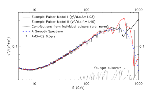
Figure 1: The AMS-02 positron fraction measurement (data points) of Ref.  Aguilar et al. (2019a). We show in the solid black and red lines the positron fraction from two pulsar population models, originally produced in Cholis and Krommydas (2022a) and in the dashed blue line a smooth positron fraction as that coming from an annihilating dark matter particle. The contribution of individual pulsars is shown by the dotted lines. Younger pulsars contribute at higher energies. The flux normalizations from individual pulsars are taken to be arbitrary, just to showcase the contributions of some pulsars and are picked to be higher for the older pulsars in order for them to appear within plot (see text for more details).

II Data and Methodology

II.1 Cosmic-ray observations

We use observations by AMS-02 on the cosmic-ray positron fraction and positron and electron flux spectra spanning from 5 GeV to 1 TeV Aguilar et al. (2019a, b). While Refs. Aguilar et al. (2019a, b), measure these spectra down to 0.5 GeV in energy, we ignore the 0.5 to 5 GeV range. These lower energies are dominated by uncertainties on the modeling of solar modulation that cosmic-rays undergo as they propagate inward through the heliosphere and also by the uncertainties relating to the production of electrons and positrons from inelastic collisions of cosmic-ray nuclei with the ISM gas (see e.g. Orusa et al. (2022)). Moreover, at energies $<5$ GeV, we expect no spectral features relating to the presence of any individual Milky Way pulsar, as the number of contributing sources is too large and the resulting spectra from pulsar populations are very smooth Malyshev et al. (2009); Profumo (2011); Grasso et al. (2009); Cholis et al. (2018a); Orusa et al. (2021); Cholis and Krommydas (2022a).

For our power-spectrum analysis, we rely on the positron fraction spectra from AMS-02 Aguilar et al. (2019a), that is shown in Fig. 1. The positron fraction has smaller overall errors compared to the positron flux measurement of Aguilar et al. (2019b), as some of the systematic errors cancel out in taking a ratio of cosmic-ray fluxes. Instead, for our cross-correlation, we take the published AMS-02 electron and positron spectra of Ref. Aguilar et al. (2019a) and Ref. Aguilar et al. (2019b) respectively. These measurements are also shown in Fig. 2.

II.2 Methodology

The cosmic-ray electron and positron fluxes that we simulate have three components. The first, is the primary electrons accelerated by SNRs. The second one, is the secondary electrons and positrons produced at inelastic collisions in the ISM. Finally, local galactic pulsars produce cosmic-ray electrons and positrons.

II.2.1 Simulations of Milky Way pulsars

As a basis for the range of possibilities of spectral features from pulsars, we use the results of Ref. Cholis and Krommydas (2022a) that produced a library of simulations on the Milky Way pulsar population. These simulations account for the discreteness of these sources both in position and age, uncertainties in the pulsar birth rate and the fact that each pulsar has a unique initial spin-down power, within a distribution that can be constrained by radio observations Faucher-Giguere and Kaspi (2006); Manchester et al. (2005); http://www.atnf.csiro.au/research/pulsar/psrcat . Moreover, these simulations account for uncertainties in the pulsars’ time-evolution related to the pulsars’ braking index and characteristic spin-down timescale. From each pulsar only a fraction $\eta$ of its rotational spin-down power gets converted to cosmic-ray electrons and positrons injected to the ISM. Moreover, each pulsar has a unique value on the conversion fraction $\eta$. Uncertainties on that fraction $\eta$ and on the properties that describe the underlying distribution of $\eta$ for a population of pulsars have been included in the simulations of Ref. Cholis and Krommydas (2022a) that we use. Also, the injected electrons and positrons from each pulsar are described by a unique injection spectral index $n$ within a range of allowed values. We assume that at injection the differential spectrum of cosmic rays is $dN/dE\propto E^{-n}\cdot exp\{-E/10\;\textrm{TeV}\}$. Finally, these simulations account for the fact that cosmic rays propagate through the ISM and the volume affected by the solar wind, the heliosphere. Uncertainties on the cosmic-ray propagation uncertainties through the ISM and the heliosphere are included.

For the propagation through the ISM, the most relevant uncertainties are those of cosmic-ray diffusion and energy losses related to synchrotron radiation and inverse Compton scattering. Cosmic rays are assumed to propagate within a cylinder of radius 20 kpc and of half-height $z_{L}$ that is between 3 and 6 kpc. That cylinder has its center at the center of the Milky Way. Diffusion is assumed to be homogeneous and isotropic, described by a diffusion coefficient $D(R)=D_{0}(R/(1\;\textrm{GV}))^{\delta}$, where $\delta$ is between 0.33 and 0.5, with the limiting values describing Kolmogorov and Kraichnan diffusion respectively Kolmogorov (1941); Kraichnan (1967, 1970). At the cosmic-ray energies of interest, i.e. $\simeq$1GeV to 1 TeV, for the inverse Compton scattering the Thomson cross section Klein and Nishina (1929) approximates well the Klein-Nishina one Blumenthal and Gould (1970). As a result the electron/positron rate of energy losses can be simply written as $dE/dt=-b(E/(1\,GeV))^{2}$, where $b$ scales proportionally to the energy density in the cosmic microwave background photons, the interstellar radiation field photons and the local galactic magnetic field.

Our models also include the effects of diffusive reacceleration Seo and Ptuskin (1994) and convective winds in the ISM. All the relevant ISM propagation assumptions are tested to measurements by AMS-02 and Voyager 1 on the cosmic-ray hydrogen, and AMS-02 measurements of the cosmic-ray spectra of helium, carbon and oxygen fluxes and the beryllium-to-carbon, boron-to-carbon and oxygen-to-carbon ratio spectra studied in Cholis et al. (2022a). The properties of the ISM in those simulations are also in agreement with results from Refs. Trotta et al. (2011); Pato et al. (2010). In addition, the electron and positron spectral measurements from AMS-02, CALET and DAMPE are used in Cholis and Krommydas (2022a) to set constrains on the ISM local propagation. For the secondary fluxes GALPROP v54 Strong and Moskalenko (1998); http://galprop.stanford.edu/. , has been used. Finally, to include the effects of cosmic-ray propagation through the heliosphere which results in the solar modulation of all cosmic-ray spectra at energies bellow 50 GeV, we use the time-, charge- and rigidity-dependent formula for the solar modulation potential from Cholis et al. (2016), including recent analyses results from Cholis et al. (2022b); Cholis and McKinnon (2022).

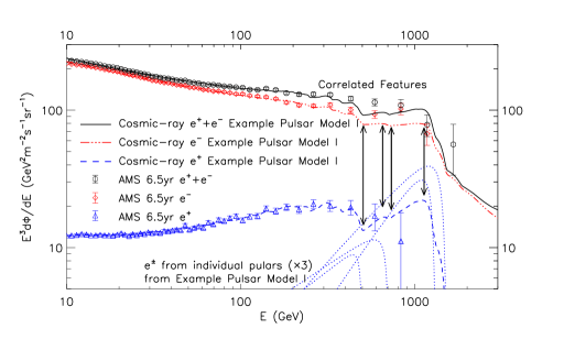
Figure 2: The predicted electron flux (red dashed-dotted line) and positron flux (blue dashed line) from an example pulsar population model. The AMS-02 electron and positron flux measurements are shown by the red and blue data points respectively. For a small number of the most prominent members of the pulsar population, we show in dotted blue lines the predicted electron and positron fluxes at Earth. In the black line and AMS-02 data points, we give the combined $e^{+}+e^{-}$ flux.

In Figure 2, we give an example of the simulated electron cosmic-ray flux, the positron cosmic-ray flux and the combined electron plus positron flux, from a population of pulsars including primary and secondary cosmic-ray fluxes. We also provide the relevant spectral data from AMS-02. There are many more cosmic-ray electrons as the simulation includes the primary electron component from SNRs that exists only in electrons. Secondary fluxes are taken to be equal between electrons and positrons. For a few powerful and middle-aged to young pulsars (ages of $O(10^{5})$ yr or younger), we also show their individual simulated fluxes. Pulsars are taken to contribute equal fluxes of cosmic-ray electrons and positrons. Powerful pulsars give spectral features to both the electron and the positron fluxes that coincide in energy. This is a property that we will use in our cross-correlation analysis.

As is showcased in Figs. 1 and 2, spectral features from individual pulsars appear at energies above $\sim 50$ GeV . In Ref. Cholis and Krommydas (2022a), about $7.3\times 10^{3}$ unique Milky Way pulsar simulations were created to account for the combination of the described above astrophysical uncertainties. Each of these simulations contained between $6\times 10^{3}$ and $20\times 10^{3}$ unique pulsars within 4 kpc from the Sun, created over the last 10 Myr. Of these $7.3\times 10^{3}$ local Milky Way pulsar population simulations, 567 simulations can fit the cosmic-ray positron fraction of AMS-02 above 15 GeV within 2$\sigma$ from a value of $\chi^{2}$/d.o.f. = 1. There are 44 energy bins in the AMS-02 positron fraction measurement of Ref. Aguilar et al. (2019a), between 15 and 1 TeV; and are fitted by seven free parameters. These parameters account for the uncertainties on the normalizations of primary cosmic rays, secondary cosmic rays and cosmic rays from pulsars. They account also for uncertainties on the injection spectral indices of the comic-ray primaries and secondaries and on the modeling of solar modulation (see Ref. Cholis and Krommydas (2022a) for more details). The simulations that are within 2$\sigma$ from an expectation of $\chi^{2}$/d.o.f. = 1, have a $\chi^{2}$/d.o.f.$\leq 1.290$ on the positron fraction. In the remainder of this work, we use those 567 simulations as a basis on studying the kind of spectral features pulsar populations consistent with the current cosmic-ray measurements can give. We note that these 567 simulations are also within 2$\sigma$ from an expectation of $\chi^{2}$/d.o.f. = 1 to the positron flux measurement by AMS-02 Aguilar et al. (2019b) and the electron plus positron measurements by AMS-02, CALET and DAMPE Aguilar et al. (2021); Adriani et al. (2018); Ambrosi et al. (2017). The positron fraction combined statistical and systematic errors are the smallest among those observations and thus provide the main dataset in excluding Milky Way pulsar simulations. These simulations are used for both the power-spectrum analysis on the positron fraction and subsequently the cross-correlation of the predicted electron and positron fluxes. We also check the Milky Way pulsar simulations that were within 3$\sigma$ from an expectation of $\chi^{2}$/d.o.f. = 1, on the positron fraction, i.e. have a $\chi^{2}$/d.o.f.$\leq 1.467$ and find that our results are qualitatively the same.

II.2.2 Power Spectrum on the Positron Fraction

While our simulations have underlying spectral features, statistical noise prominent in the high-energy cosmic-ray bins, will also cause fluctuations. That is true even if the underlying positron fraction spectrum is a smooth one, as the one depicted by the blue dashed line of Fig. 1. We want to evaluate how often the signal from underlying high-energy spectral features is above the statistical noise. Building on the work of Refs. Malyshev et al. (2009); Cholis et al. (2018b), we want to use a power-spectrum analysis. We want to dissociate our work on the presence of spectral features in the cosmic-ray data, from any particular energy bin. We do not know the properties of the entire local population of Milky Way pulsars -observing only a fraction of them through electromagnetic observations- nor the exact properties of the local ISM. Thus, we can not predict at what exact energies these spectral features will appear. Our analysis only relies on the fact that a large fraction of the Milky Way pulsar simulations that we use predict some prominent features at the higher energies.

For each of the 567 pulsar astrophysical simulations, we generate 10 observational/mock realizations, i.e. we add noise on our simulations using the same energy bins and statistical $\%$ errors from Ref. Aguilar et al. (2019a). The noise-related fluctuations in some cases enhance and in other cases suppress the underlying spectral features. While the current measurement of the positron fraction seems (by eye) to suggest that the source of positrons with energies greater than $\simeq 500$ GeV is phasing out, statistically a positron fraction that has a plateau above 500 GeV, or even increases is still consistent with the data of Aguilar et al. (2019a). We want to avoid any bias in our results from the large scale (in energy) evolution of the positron fraction. To do that, from each observational realization, we subtract its relevant smoothed spectrum and evaluate the power-spectral density (PSD) on its residual spectrum. For each positron fraction realization, its smoothed spectrum is evaluated by convolving with a gaussian function, whose width increases with energy. In doing that, we remove power from large scales in energy, i.e. low modes in the power spectrum. This is an important point, as in an actual analysis on the observed by AMS-02 positron fraction measurement, instrumental systematics that may span multiple energy bins are also removed in this manner. An example of such a systematic may be a misestimate of the instrument efficiency or cosmic-ray contamination.

To evaluate the PSD on the residual positron fraction spectrum, we take as the equivalent of the “time” parameter to be $ln(E/\textrm{GeV})$. Approximately the energy binning of the AMS-02 data is done in equal intervals of $ln(E)$ up to $\sim 200$ GeV. For this analysis where we use observational/mock realizations, we take the energy binning to be on exactly equal bins in the $ln(E)$-space. The specific logarithmic energy binning we assume is,

$$ln(E_{i}/\textrm{GeV})\equiv x_{i}=x_{0}+a\cdot i,$$ (1)

with $x_{0}=1.6564$ (5.24 GeV) and $a=0.077$. This is a slightly more dense energy binning than AMS-02, but only at the higher energies. Such a binning may be used in measurements that include longer observation times than the currently published 6.5-year ones. When comparing to current data, we go up to $i=59$ (492 GeV). We calculate the PSDs for each of the 567$\times$10 observational/mock realizations that include noise, giving a scatter on the PSDs of these realizations evaluated for any given underlying astrophysical simulation.

We need to compare the PSDs of the 5670 observational realizations from our pulsar population simulations to what the PSDs are expected to be by just having noise on the residual positron fraction spectra. To do that, we take the AMS-02 measurement of the positron fraction, and convolve it with the same gaussian function used to derive the smoothed positron fraction simulated spectra for the 567 pulsar population simulations. That gives us the smooth AMS-02 positron fraction spectrum. We then use that smooth spectrum and add noise on it, following the same procedure as for the pulsar population simulations. We create 1000 simulated AMS-02 positron fraction measurements. From each of those simulated measurements, we subtract the smooth AMS-02 positron fraction spectrum and then on these residuals we evaluate 1000 PSDs using the same binning of Eq. 1. These 1000 PSDs give us the PSD-ranges due to the statistical noise.

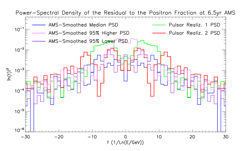
Figure 3: The power-spectral density of the residual cosmic ray positron fraction as a function of frequency, where frequency is taken to be $1/ln(E/(1\;\textrm{GeV}))$. Assuming that the positron fraction is a smooth featureless function with fluctuations arising due to noise, we give the expected PSD as a fraction of frequency. That is shown in the blue, pink and purple lines for the simulations with the median total power in the PSD, for the 95-percentile (95$\%$) higher total power in the PSD and for the $95\%$ lower total power in the PSD respectively (see text for details). In the green and red lines we showcase that if the pulsars have inherent spectral features, those will remain as fluctuations in the residual positron fraction spectrum and even with noise present, can give an enhanced PSD in a certain frequency range (modes 3-13 in these examples).

In Fig. 3, we plot three PSDs of the residual to the simulated positron fraction, using the 6.5-year data for the noise Aguilar et al. (2019a). Assuming that the positron fraction is a smooth featureless function (as the one shown in Fig. 1 by the blue dashed line), with only noise causing fluctuations around it, we plot the expected PSD $|h(f)|^{2}$ as a faction of “frequency” $f=1/ln(E/\textrm{GeV})$. Ranking the 1000 AMS-02 realizations based on the total power i.e. $\Sigma_{i=-30}^{i=+30}|h(f_{i})|^{2}$, we can identify the AMS-02 realization that has a median value on its total power. This is given by the blue line in Fig. 3. By the same ranking, we identify the AMS-02 realization that is at the 95-percentile higher range in terms of its total power (95$\%$ higher PSD), given by the pink line and the realization that is at the 95-percentile lower range in terms of its total power (95$\%$ lower PSD), given by the purple line. Finally, we plot the PSDs evaluated from for two pulsar populations (red and green lines). We noticed that a significant fraction of our pulsar populations simulations have an enhanced PSD in modes 3-13, compared to the noise PSD ranges, which we will explore in more detail in section III.

In addition, for every one of the 60 modes that we use, we rank the 1000 coefficients from the 1000 AMS-02 noise realizations. We use the 68$\%$ ranges to derive the $1\sigma$ error-bars per mode. We note that we do not expect any correlations between modes. We can use those $1\sigma$ error-bars per PSD mode, to calculate a $\chi^{2}$ fit on each of the PSDs derived from our pulsar populations. Like with the total power we can rank the 1000 mock realizations of the AMS-02 smooth parametrization in terms of the $\chi^{2}$ quality fit and present the median among those 1000 realizations. We can do the same to get the $68\%$, $90\%$ and $98\%$ ranges for the 1000 mock realizations of the AMS-02 with noise. We use these ranges again to compare in terms of their $\chi^{2}$ quality, the expected PSDs of the pulsar population astrophysical realizations to the PSDs we get just due to statistical noise. This is an alternative way to check if pulsar related features can give a signal in the PSD that is above the noise.

II.2.3 Cross-correlating the Electron and Positron Spectra

Like with the power-spectrum analysis, we are focused in comparing the small-scale features of the electron and positron fluxes coming from pulsars to random noise fluctuations. To study these features, rather than the full electron and positron flux spectra, we need to evaluate the residual spectra after subtracting a smooth function that describes well the large scale energy-dependence of these spectra. The smoothed models that we use are crucial to the analysis.

The AMS-02 collaboration has provided a model/parameterization for each of the electron and positron spectra Aguilar et al. (2019a, b). While their parameterization works for the positron spectrum, it overpredicts the electron observations at the lower energies as shown in the residuals in Fig. 4. We focus on energies above 10 GeV as below that energy, features from individual pulsars are not expected. In Fig. 4, in the top panel we show the positron and electron measurements above 10 GeV as well as the parameterizations provided by the AMS-02 collaboration. As we show in the bottom panel of Fig. 4, (blue line) once removing from the AMS-02 data the smooth parameterization, the resulting residuals span only a small number of energy bins. The most prominent remaining features in positrons are seen around 12 GeV and around 21 GeV. Those may be related to physical processes from further away distances than few kpc away from the Sun as suggested recently in Cholis and Krommydas (2022b). However, in the electrons we don’t see as prominent features . In the bottom panel of Fig. 4, we show (in red) the residual cosmic-ray electron flux once removing the smooth spectrum as parameterized by AMS-02. The residual flux systematically underpredicts the observed flux between 20 and 80 GeV even if its overall quality of fit has a $\chi^{2}/\textrm{d.o.f.}<1$. For that reason we performed a $\chi^{2}$-fit, deriving slightly different values of the parameters within the same parametrization given in Table 1. Our choice fits the overall spectra better and gives residuals that are more localized in energy. The difference between the AMS-02 parameterization and the alternative one is too small to show up in the top panel of Fig. 4, but can be seen in the bottom panel. The orange line does fluctuate around zero, however in electrons with energy less than 40 GeV there are still neighboring bins that may be correlated.

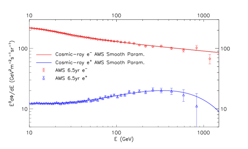
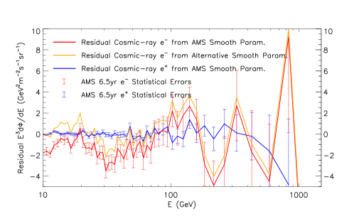
Figure 4: Top panel: the AMS-02 electron (red) and positron (blue) flux measurements and their respective smooth parameterizations from Refs. Aguilar et al. (2019a, b). Bottom panel: the residual electron and positron fluxes. For the electrons we derive an alternative smooth parameterization (orange) that allows us to then study the residual spectra upon which our cross-correlation analysis is performed. We also show the statistical errors for the electron and positron measurements after 6.5 years. We do not over-plot statistical errors for the alternative smooth spectrum electron parameterization as they are the same in size as the red ones.

Here, for clarity on the assumptions that we use, we repeat what the parameterizations from Refs. Aguilar et al. (2019a, b) are. The positrons smooth spectrum is given by,

$$\frac{d\Phi_{e^{+}}}{dE}(E) = \frac{E^{2}}{\hat{E}^{2}}[C_{d}(\hat{E}/E_{1})^{\gamma_{d}}$$ (2)

$$+\;C_{s}(\hat{E}/E_{2})^{\gamma_{s}}\cdot exp\{-\hat{E}/E_{s}\}].$$

The parameter $\hat{E}$ is energy dependent and equal to $\hat{E}=E+\phi_{e^{+}}$, where $\phi_{e^{+}}=1.10$ GeV. The other parameters of Eq. 2, are $C_{d}=6.51\times 10^{-2}[\textrm{m}^{2}\,\textrm{s}\,\textrm{sr}\,\textrm{GeV}]^{-1}$, $\gamma_{d}=-4.07$, $C_{s}=6.80\times 10^{-5}[\textrm{m}^{2}\,\textrm{s}\,\textrm{sr}\,\textrm{GeV}]^{-1}$, $\gamma_{2}=-2.58$, $E_{1}=7.0$ GeV, $E_{2}=60.0$ GeV and $E_{s}=810$ GeV.

The electrons smooth spectrum is given by,

$$\frac{d\Phi_{e^{-}}(E)}{dE} = \frac{E^{2}}{\hat{E}^{2}}\left[1+\left(\frac{\hat{E}}{E_{t}}\right)^{\Delta\gamma_{t}}\right]^{-1}$$ (3)

$$\times \left[C_{a}\left(\frac{\hat{E}}{E_{a}}\right)^{\gamma_{a}}+C_{b}\left(\frac{\hat{E}}{E_{b}}\right)^{\gamma_{b}}\right].$$

The parameter $\hat{E}$ is also energy dependent and equal to $\hat{E}=E+\phi_{e^{-}}$. In Table 1, we give the values of the parameters in Eq. 3 for the AMS-02 and our alternative parameterizations. The values for $E_{a}$ and $E_{b}$ are fixed in both the results of Aguilar et al. (2019a) and our analysis. We created a $\chi^{2}$ per degree of freedom function and optimized it with dual annealing. This method was chosen as it can fit several parameters at once and the function need not be linear to use it. This method is stochastic, thus, each time it runs, we receive slightly different values for these parameters.

Parameter	AMS-02 value	Alternative value
$\phi_{e^{-}}$ (GeV)	0.87	0.87
$E_{t}$ (GeV)	3.94	3.94
$\Delta\gamma_{t}$	-2.14	-2.15
$C_{a}$ ($[\textrm{m}^{2}\,\textrm{s}\,\textrm{sr}\,\textrm{GeV}]^{-1}$)	$1.13\times 10^{-2}$	$1.12\times 10^{-2}$
$E_{a}$ (GeV)	20	20
$\gamma_{a}$	-4.31	-4.31
$C_{b}$ ($[\textrm{m}^{2}\,\textrm{s}\,\textrm{sr}\,\textrm{GeV}]^{-1}$)	$3.96\times 10^{-6}$	$3.93\times 10^{-6}$
$E_{b}$ (GeV)	300	300
$\gamma_{b}$	-3.14	-3.14

Table 1: The parameters describing the smooth function for the cosmic-ray electron flux in Eq. 3. In the second column we repeat the information from Ref. Aguilar et al. (2019a).

Under the original parameters, for energies above 5 GeV we get a $\chi^{2}$/d.o.f. of 0.65 for the electron data once adding in quadrature the statistical and systematic errors. Under the new parameters, for the same energy range, we get instead a $\chi^{2}$/d.o.f. of 0.37. We note however, that on the cross-correlation analysis we only retain the statistical errors that are shown in Fig. 4 (bottom panel). The systematic/instrumental errors span several energy bins, unlike the spectral features we are searching for and thus can be ignored for the cross-correlation purposes.

The cross-correlation function Kido (2015), is an operation which takes discrete functions $x(n)$ and $y(n-m)$, and creates a function $r_{xy}(m)$ which describes the relatedness of each point $n$ as a function of a shift variable $m$. In our specific case we define a similar type of cross-correlation function $r_{xy}(m)$ described by,

$$r_{xy}(m)=\frac{1}{L-|m|}\begin{cases}\Sigma_{n=m}^{L-1}\frac{x(n)y(n-m)}{\sigma_{x}(n)\sigma_{y}(n-m)}\;\;\textrm{for $m\geq 0$}\\ \Sigma_{n=0}^{L-1+m}\frac{x(n)y(n-m)}{\sigma_{x}(n)\sigma_{y}(n-m)}\;\;\textrm{for $m<0$}\end{cases}$$ (4)

$L$ is the number of discrete data points for which we know $x$ and $y$ functions; while $\sigma_{x}$ and $\sigma_{y}$ are the respective errors (standard deviations). In our case $L=50$ starting our analysis above 10 GeV and going up to the last data point in positrons (700-1000 GeV). $x(n)$ and $y(n)$ are respectively the positron and electron residual spectra shown in Fig. 4 (bottom panel) i.e. $E^{3}d\Phi(E)/dE$ (in $[\textrm{m}^{2}\,\textrm{s}\,\textrm{sr}]^{-1}\textrm{GeV}^{2}$). $\sigma_{x}$ and $\sigma_{y}$ the respective systematic errors. The parameter $n$ is set to 0 for the bin centered at 10.67 GeV, covering the cosmic rays with energy of 10.32 to 11.04 GeV. The maximum range of energies tested is from 10 GeV and up to 1.0 TeV. A positive shift $m$, represents shifting the electron flux to lower energies. We test up to values of $|m|=24$, however the large shifts suffer from noise as the number of bins drops down to half the original number. We do not show results for larger shifts as there is no physical reason to see any correlation between bins separated many 10s to 100s of GeV from each other.

We note, an important caveat about the specific version of Eq. 4 that we use. Conventional cross-correlation would require in the fraction of Eq. 4, to have instead of $x(n)y(n-m)/(\sigma_{x}(n)\sigma_{y}(n-m))$, the fraction $(x(n)-\bar{x})(y(n-m)-\bar{y})/(\sigma_{x}(n)\sigma_{y}(n-m))$. That would give a well-defined cross-correlation that would give correlation coefficients $r_{xy}(m)$ within $[-1,+1]$. However, that would require to evaluate averages for $x(n)$ and $y(n)$, where different values of $n$ are not different instances of a time-series but different energies, where different physical phenomena occur. Pulsars are most dominant at high energies while secondary cosmic rays are more important at the lower energies. Our Eq. 4 uses the residual spectra that still may have $\bar{x}\neq 0$ and $\bar{y}\neq 0$. Our residual spectra may still contain features spanning a few bins as a pulsar population may predict pulsars giving partially overlapping spectral features. If that is the case, we don’t want this information to be completely lost. By subtracting from a smooth function that describes the overall spectral evolution, while not removing the average of the entire 10-1000 GeV range we achieve that goal. Also, removing the $\bar{x}$ and $\bar{y}$ would associate in the residual spectra physical conditions at 10 GeV to 1000 GeV and as at higher energies the noise is very large would make our results overly sensitive to the exact measurements at the highest energy bins. Thus, formally our Eq. 4, can give a correlation coefficient $r_{xy}(m)$ that takes values beyond the range of $[-1,+1]$. We also note that the $\sigma_{x}$ and $\sigma_{y}$ are not the standard deviations evaluated from all the $x$ and $y$ measurements. Each point $x(n)$ and $y(n)$ has its own uncertainty, directly related to the statistical noise of AMS-02 at that energy bin, i.e. to the number of positron and electron cosmic rays detected within a specific energy range. As the AMS-02 keeps making observations, these statistical errors will become smaller. If there is an underlying correlation signal this will show up by an increasing $r_{xy}(m)$ with observation time around a specific range of $m$ values.

In practice, for our pulsar population simulations the chance of getting a $r_{xy}(m)$ beyond the range of $[-1,+1]$ is extremely small and when it happens it has to do with difficulty in evaluating the proper residual spectra. However, in the case of the actual AMS-02 measurements, evaluating a proper residual spectrum is still a challenge at the lower electron energies.

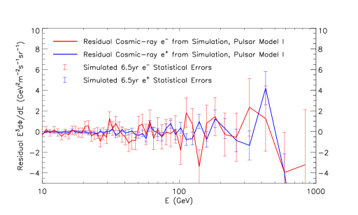
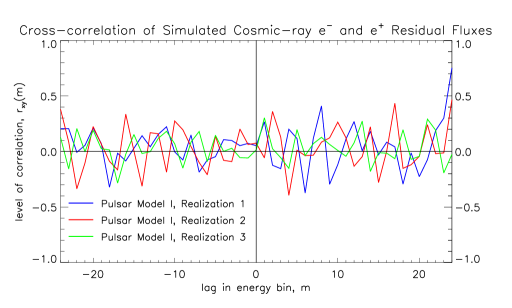
Figure 5: Top panel: like with Fig. 4 (bottom panel), the residual electron (red) and positron (blue) fluxes from one realization of the Milky Way pulsar population Model I. The statistical errors are simulated for 6.5 years of AMS-02 measurements. Bottom panel: the cross-correlation function between the electron and positron residual fluxes for three different observational realizations of the same underlying pulsar population (Model I). Pulsars give a peak of cross-correlation signal around $m=0$ to +1.

The dependence of the $r_{xy}(m)$ correlation coefficient as a function of the shift $m$ is what we study here. To see if there can be a cross-correlation signal related to pulsars in the AMS-02 measurements, we need to compare to the expectations from our pulsar population simulations. In Fig. 5, we show, as an example the residual electron and positron spectra from one observational realization of a Milky Way pulsar population,“Model I” simulation. We remind the reader that we create 10 observational realizations per Milky Way pulsar population simulation. These observational realizations contain the information of statistical noise for 6.5 years of AMS-02 observations. For each of them, we then evaluate the smoothed electron and positron spectra by convolving the simulated spectra with the same kind of gaussian function described in II.2.2. Then, we subtract from the simulated realization electron and positron spectra their equivalent smoothed spectra, getting the residual electron and positron spectra. It is these residual spectra that we cross-correlate. In the bottom panel of Fig. 5, we show the cross-correlation coefficient $r_{xy}(m)$ as a function of $m$, for three observational realizations of the same underlying pulsar population “Model I” simulation. The blue line on the bottom panel, is the one calculated from cross-correlating the residual spectra of the top panel on Fig. 5. For the cross-correlation, we use the same energy binning as the AMS-02 results of Aguilar et al. (2019a, b). We do not need the energy bins to be equally separated (in $log(E)$) as we need for the power-spectrum analysis of section II.2.2. We note that a peak of cross-correlation coefficient occurs around $m$=0 or +1, typically being between $0$ and $+3$. A positive $m$ value for the peak suggests that the pulsar features on the electrons typically appear to be shifted by one bin at lower energies. In section III, we describe these and other properties of the cross-correlation signals we expect from pulsar populations for the entire set of simulations.

III Results

III.1 Power-Spectrum Analysis on Pulsar Population Simulations

We start with the results of the power-spectrum analysis on the pulsar population simulations. As we described in section II.2.2, using the 1000 AMS-02 mock positron fraction simulations we can calculate $1\sigma$ error-bars per each of the 60 PSD modes. From them, we can calculate the $\chi^{2}$ fit on each of the pulsars PSDs. In Fig. 6, we show the PSD $\chi^{2}$-distribution (red diamonds) from each of the 10 observational realizations of our 567 pulsar population simulations. Each pulsar population simulation is in a different position on the $x$-axis. These are ranked from left to right starting from the model that provides the best fit the positron fraction spectrum, with all of them being within a 2$\sigma$ from an expectation of $\chi^{2}$/d.o.f. = 1 to the positron fraction (and flux) measurement. Given that we rank our models from better to worse fit, there is no clear pattern between the quality of fit that models provide to the observed positron fraction spectrum and their respective PSD $\chi^{2}$/d.o.f.. The 1000 mock realizations of the AMS-02 smooth parametrization for the positron fraction, can be ranked in terms of their PSD $\chi^{2}$/d.o.f. (our $y$-axis). From there we get the respective $68\%$, $90\%$ and $98\%$ (two-sided) ranges, for the case where only noise is present, i.e. no underlying small-scale features. These are shown in the three different shades of blue in Fig. 6. By comparing the red diamonds to the blue ranges, we notice that pulsar population simulations have a tendency for larger values of PSD $\chi^{2}$s. We find that with the 6.5-years of sensitivity 1.8$\%$ (7.2$\%$) of the 5670 observation realizations lie outside the $99\%$ ($95\%$) upper band end, i.e. above $y$-axis from the $90\%$ and $98\%$ ranges plotted in Fig. 6. This information is also given in Table 2. Calculating the PSD on the observed AMS-02 residual positron fraction gives us the black line, which is very close to the median noise mock simulation (blue dashed line). Thus, with the current data there is no indication in the AMS-02 data for a deviation from a smooth spectrum, just relying on the PSD $\chi^{2}$ criterion.

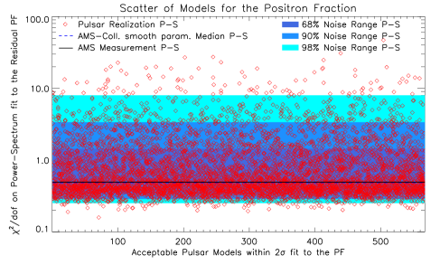
Figure 6: The scatter of the simulated Milky Way pulsars observational realizations in the PSD $\chi^{2}$/d.o.f., evaluated from their residual positron fraction spectrum. We plot 10 realizations (in red diamonds) for each of the 567 pulsar population astrophysical simulations that are consistent within $2\sigma$ to the positron fraction measurement (see section II.2.1 for details). The blue bands include the noise ranges for the PSD $\chi^{2}$/d.o.f.. The black line gives the PSD of the AMS-02 measurement after 6.5 years. The black line (measurement) overlaps very well with the median expectation of $\chi^{2}$/d.o.f. coming from a smooth spectrum with noise added (blue dashed line). This shows no evidence for features within the 6.5-year data.

Type of ranking	$\%$inc. f.	$\%$inc. f.	$\%$inc. f.
	(16$\%$)	(5$\%$)	(1$\%$)
$\chi^{2}/$d.o.f. on Power Spectrum	19.8	7.2	1.8
$\Sigma_{i=-30}^{i=+30}|h(f_{i})|^{2}$	42.0	23.7	7.6
1 - ($\Sigma_{i=-15}^{i=+15}|h(f_{i})|^{2}$/$\Sigma_{i=-30}^{i=+30}|h(f_{i})|^{2}$)	22.8	9.7	2.9

Table 2: The potential to observe power from small-scale features to the residual AMS-02 positron fraction after 6.5 years of observations. We use the energy range between 5 and 500 GeV, with $f=1/ln(E/(1\;\textrm{GeV}))$ in the range of $\pm 30$, i.e $\pm 1/2$ the number of logarithmically spaced E-bins. For the first two criteria used to rank our 5670 Milky Way pulsar realizations, we give the fraction in $\%$, of these realizations that fall inside the the upper 16$\%$, 5$\%$ and 1$\%$ noise ranges (“$\%$inc. f.”). For the third criterion, we give the lower 16$\%$, 5$\%$ and 1$\%$ noise ranges.

While the $\chi^{2}/$d.o.f. on the PSD criterion separates some of the pulsar population simulations from the simulations of noise around a smooth spectrum, it still leaves a significant level of overlap between the two. As shown in Table 2, for the overwhelming number of pulsars simulations their features would not give a $\chi^{2}/$d.o.f. fit much different to what noise would. For that reason we seek alternative criteria to break the two sets of simulations apart.

In Fig. 3, we showed two Milky Way pulsars simulations that compared to noise, give an increased total power in the power spectrum, i.e. a larger $\Sigma_{i=-30}^{i=+30}|h(f_{i})|^{2}$. In Fig. 7 (left panel), we plot the scatter of the 5670 realizations of pulsar population simulations in terms of that total power. Our $x$-axis is as with Fig. 6, i.e. ranks the models from better to worse, in terms of their ability to fit the AMS-02 positron fraction measurement. There is no clear pattern on the total power in the PSD (our $y$-axis) a pulsar population simulation gives versus the quality of fit it has on the AMS-02 data. All these simulations provide a relatively good quality of fit to the AMS-02 positron fraction spectrum, as they give up to a $\chi^{2}/$d.o.f.=1.29. Simulations that would predict very large spectral features are excluded. There is a large scatter along the $y$-axis, $\Sigma_{i=-30}^{i=+30}|h(f_{i})|^{2}$ values. This is directly related to the relatively large noise present in that energy range. We tried an alternative, narrower energy range and concluded that using the 5-500 GeV data is close to the optimal choice in searching for signals of spectral features given, the span of possible pulsar models explaining the data. Even with the large scatter along the $y$-axis, our pulsar population simulations give a larger total power than the regular noise around a smooth positron fraction spectrum does. In the blue shaded bands of the left panel of Fig. 6, we give the $68\%$, $90\%$ and $98\%$ two-sided ranges on the $\Sigma_{i=-30}^{i=+30}|h(f_{i})|^{2}$ from the 1000 noise simulations. We find that of the 5670 observation realizations, 7.6$\%$ and 23.7$\%$ lie outside the $99\%$ and $95\%$ upper band end along the respective $y$-axis. Using the total power is quite a more sensitive criterion in separating the pulsar population simulations from noise. We note that still a significant fraction of pulsar population simulations, predict too little additional structure in the 5-500 GeV range of the positron fraction, to give a signal in the PSD.

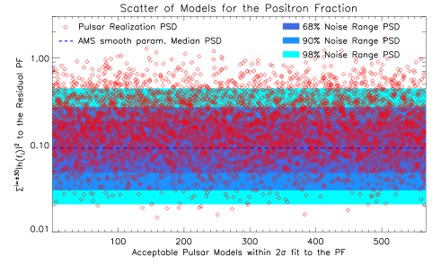
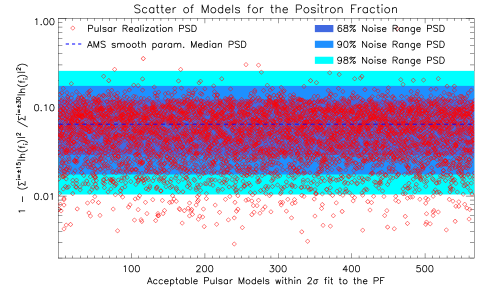
Figure 7: As with Fig. 6, the scatter of the simulated Milky Way pulsars observational realizations, plotted by different characteristics of their PSDs. In red diamonds, we show 10 realizations from each of the 567 pulsar population simulations used. Left panel: each diamond gives the total PSD power $\Sigma_{i=-30}^{i=+30}|h(f_{i})|^{2}$, for each realization. The blue bands show the ranges of PSD total power for an underlying smooth spectrum with the addition of AMS-02 noise and the blue dashed line the median expectation. Spectral features from pulsars increase the total PSD power, as shown by the overall shift of the diamonds with respect to the blue bands. Right panel: each red diamond gives the ratio of PSD power in the lower half modes to the total PSD power. To show how the pulsars predictions differ from that of noise, we plot the 1 - ($\Sigma_{i=-15}^{i=+15}|h(f_{i})|^{2}$/$\Sigma_{i=-30}^{i=+30}|h(f_{i})|^{2}$. As with the left panel, the blue bands show the AMS-02 noise relevant ranges and the blue dashed line the median expectation. Pulsars predict a greater fraction of PSD power in the lower modes than regular noise. The diamonds are shifted to lower values in the $y$-axis with respect to the blue bands (see also text and Table 2).

In the right panel of Fig. 6, we explore further the point that pulsar realizations have a larger fraction of their power in low frequency $f=1/ln(E/(1\;\textrm{GeV}))$ modes, compared to noise simulations. That is directly related to the fact that pulsars predict spectral features that span only a small number or energy bins. Our $x$-axis is the same as with the left panel on the same figure (unique pulsar population simulations that fit the positron fraction). Our $y$-axis, gives the 1 - ($\Sigma_{i=-15}^{i=+15}|h(f_{i})|^{2}$/$\Sigma_{i=-30}^{i=+30}|h(f_{i})|^{2}$). Pulsars with a larger fraction of their power in the low modes are at the bottom of the $y$-axis. The blue bands give the two sided $68\%$, $90\%$ and $98\%$ ranges on the 1 - ($\Sigma_{i=-15}^{i=+15}|h(f_{i})|^{2}$/$\Sigma_{i=-30}^{i=+30}|h(f_{i})|^{2}$) fraction evaluated from the 1000 noise simulations. Pulsar realizations are indeed shifted to lower values of that fraction. We find that 2.9$\%$ and 9.7$\%$ of the 5670 pulsars realizations lie outside the $99\%$ and $95\%$ lower band end along the $y$-axis (see also Table 2). Finally, we note that there is no clear pattern in the goodness of fit that a pulsar population simulation has on the positron fraction spectrum and our $y$-axis value.

III.2 Cross-correlation Analysis on Pulsar Population Simulations

As we showed in Fig. 5 for pulsar model I, there is significant noise in the residual electron and positron spectra of our pulsar population simulations after 6.5 years of AMS-02 observations. This results in the correlation coefficient $r_{xy}(m)$ to randomly acquire large positive and negative values for large values of shift $m$, correlating energy bins between the two residual spectra that are far away from each other. If pulsars are the underlying source for the high energy positrons, there is only one true realization of them. Since we don’t know that, we want to search for general patterns among the many pulsar population simulations that are still in agreement with the cosmic-ray observations.

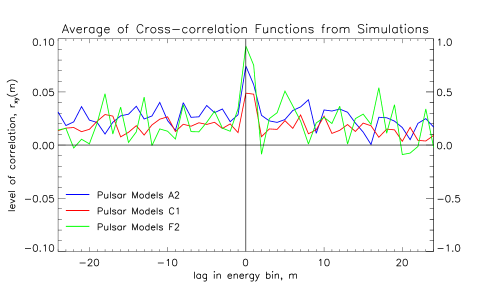
Figure 8: The averaged cross-correlation function between the electron and positron residual fluxes, evaluated from the observational realizations of many pulsar population simulations. We show the averages from the simulations built with ISM assumptions “A2”, “C1” and “F2” (see text for details).

In Fig. 8, for specific assumptions on the local ISM propagation conditions, we calculate the average of the cross-correlation functions of all realizations produced for pulsar population simulations under the same ISM assumptions. In Ref. Cholis and Krommydas (2022a), the pulsar population simulations tested to the cosmic-ray observations, were created for 12 different combinations of choices for the local cosmic-ray diffusion and averaged energy losses (see Table II of Ref. Cholis and Krommydas (2022a)). The 567 pulsar population simulations in agreement with the cosmic-ray spectral data with their 5670 observational realizations can thus be partitioned in 12 groups based on these ISM assumptions. As was shown in Ref. Cholis and Krommydas (2022a), the combination of diffusion and energy losses assumptions can have an important impact on the quality of fit pulsar population simulations give to the cosmic-ray electron and positron observations. It can also have an effect on the presence or absence of prominent spectral features, of interest in this study. In Fig. 8, the averaged cross-correlation function between the residual electron and positron fluxes is shown for three cases of ISM assumptions. In blue, we give give the averaged $r_{xy}(m)$ for the 440 realizations of pulsar population simulations produced under the “A2” ISM assumption. In the red line we give the equivalent averaged $r_{xy}(m)$ for the “C1” ISM assumption coming from 920 realizations and in green we give the averaged $r_{xy}(m)$ for the “F2” ISM assumption coming from 140 realizations. As can be seen for all averaged cross-correlation functions, they peak at $m=0$ with $m=+1$, being the second highest point.

Models “A”, take a local diffusion scale hight of $z_{L}=5.7$ away from the galactic disk. As we described in Section II.2.1, the diffusion is assumed to be isotropic and homogeneous and given by a rigidity-dependent diffusion coefficient. Models “A”, take the diffusion coefficient $D_{0}=1.40\times 10^{2}\,\textrm{pc}^{2}$/kyr at 1 GV and the diffusion index $\delta=0.33$. Models “C”, have instead $z_{L}=5.5$, $D_{0}=0.921\times 10^{2}\,\textrm{pc}^{2}$/kyr and $\delta=0.40$, i.e. slower diffusion for lower rigidity cosmic rays but also becoming faster in a more rapid manner with increasing rigidity. Finally, models “F” take $z_{L}=3.0$, $D_{0}=0.337\times 10^{2}\,\textrm{pc}^{2}$/kyr and $\delta=0.43$, i.e. assume that cosmic rays once reaching only a 3 kpc distance away from the disk they will escape. Also, models “1” take for the high energy cosmic rays their energy loss’s rate proportionality coefficient $b$ to be $b=5.05\times 10^{-6}\textrm{GeV}^{-1}\textrm{kyr}^{-1}$. This represents conventional assumptions for the local interstellar medium radiation field and magnetic field Strong and Moskalenko (1998); Moskalenko et al. (2006); Porter and Strong (2005); Porter et al. (2017); Jansson and Farrar (2012). Instead, models “2” take a higher energy loss rate with $b=8.02\times 10^{-6}\textrm{GeV}^{-1}\textrm{kyr}^{-1}$, that is still within the estimated relevant uncertainties.

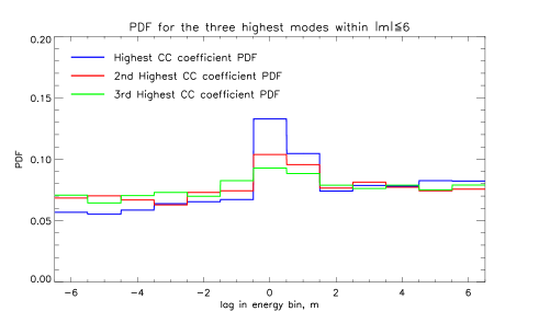
Figure 9: The distribution of the shift $m$ of the highest (blue), 2nd highest (red) and 3rd highest (green) cross-correlation coefficient evaluated from our simulations, as those presented in Fig. 5 (bottom panel). We rank only the range within $|m|\leq 6$, as higher values of $|m|$ have large noise. Each of the histogram distributions is normalized to give a total area of 1, thus these are PDFs. We use the entire sample of 5670 pulsar realizations in evaluating these PDFs.

In Fig. 9, we show for the entire set of 5670 realizations, the distribution of the location of the shift $m$, for which the three highest values of the cross-correlation coefficient $r_{xy}$ appear. We study only the region within $|m|\leq 6$, to avoid the impact of correlating the noisy data at higher energies with features at significantly lower energies. Each of our three histograms is normalized to have an area of 1, thus making these probability density functions (PDFs) for the occurrence of the highest (blue line), second highest (red line) and third highest (green line) cross-correlation coefficient value. Again, the highest value for $r_{xy}(m)$ is for $m=0$, with the second most likely shift being for $m=+1$, i.e. the pulsar features appear on the electrons to be coinciding in energy or shifted by one bin at lower energies compared to the positrons. A similar effect is seen for the second and third highest values of $r_{xy}$, but in a less prominent manner. The distribution of less high values of the $r_{xy}$ is fairly flat with $m$. As the AMS-02 collects more data and the noise gets decreased, the correlations of underlying features (if those are present) will become more easy to identify.

In Fig. 10, we show the cross-correlation analysis of the AMS-02 observations of Refs. Aguilar et al. (2019a, b), using the cosmic-ray electron and positron fluxes that we have shown in Fig. 4 and discussed in section II.2.3. Interestingly, we find a positive correlation between the residual spectra at $m=0$, with the second higher local value being at $m=+1$ as expected by our pulsar population simulations. Moreover, at the higher values of $|m|$, we do find large values of $r_{xy}$ that we associate to cross-correlating features at high energies from one residual spectrum to lower energies of the other residual spectrum.

We consider the result of Fig. 10, in association with all our expectations from the pulsar populations as we described them in this section and in section II.2.3 to be an intriguing finding. We may be at the point of detecting signs of correlated in energy spectral features in the AMS-02 data. If that is the case, then with longer observations, we will see that correlation signal become more robust and we may also see a signal of those features in the power spectrum of the residual positron fraction as discussed in sections II.2.2 and III.1.

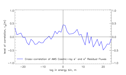
Figure 10: The cross-correlation function between the AMS-02 electron and positron residual fluxes. The vertical, guide line is at $m=0$. The correlation peaks at $m=0$ similarly to our pulsars expectation.

IV Conclusions and Discussion

In this paper, we adapt and implement a power-spectrum and a cross-correlation analysis, on the cosmic-ray measurements form the AMS-02, on the positron fraction and the electron and positron fluxes. We search for signals of underlying spectral features in these measurements. Such spectral features can exist if a population of relatively local Milky Way pulsars (or SNRs) is to explain the rising cosmic-ray positron fraction and the respective hardening of the cosmic-ray positron flux spectrum. Powerful and young to middle-aged pulsars, can be significant cosmic-ray sources on the positron fraction and electron and positron flux spectra, giving features localized in energy as we show in Figs. 1 and 2.

We implement a power-spectrum analysis on the cosmic-ray positron fraction, focusing on the capacity the current measurements have in finding a signal of spectral features from pulsars. To avoid any bias on our results from the large scale evolution of the positron fraction spectrum, we subtract the smoothed positron fraction spectrum and evaluate the power-spectral density on its residual spectrum, that would still retain the smaller scale features we are after. We do that using a vast library of Milky Way pulsar population models from Ref. Cholis and Krommydas (2022a). As we describe in more detail in section II.2.1, those simulations account for all the relevant astrophysical modeling uncertainties relating to the pulsar properties as cosmic-ray electron and positron sources, the stochastic nature of their birth, their initial power and their surrounding environment, affecting the cosmic-ray spectra they inject to the ISM. Those simulations also account for uncertainties on the characteristics of the other components of the cosmic-ray electrons and positrons, namely the primary and secondary fluxes, and finally they model the uncertainties of cosmic-ray propagation through the ISM and the heliosphere. The models that we use have already been tested in Ref. Cholis and Krommydas (2022a) for their compatibility to the electron and positron measurements made by AMS-02, CALET and DAMPE. We use only a subset of 567 simulations that give good fits to the observations from the original $\simeq 7.3\times 10^{3}$ simulations produced in Cholis and Krommydas (2022a). Moreover, to account for the presence of statistical noise in the AMS-02 positron fraction measurement, for each of the 567 pulsar population simulations we generate 10 realizations. Thus we test our hypothesis on performing a power-spectrum analysis to search for spectral features from pulsars on 5670 realizations of the positron fraction spectrum, as that would be measured after 6.5 years of observations, in agreement with the relevant published results of Aguilar et al. (2019a).

As we show in Fig. 3 and discuss in section II.2.2, by using the residual of the positron fraction between 5 and 500 GeV and calculating PSDs, there are specific “frequency” $f=1/ln(E/\textrm{GeV})$ modes, where a signal of the presence of the pulsar induced spectral features would appear. Any power-spectrum analysis would only find signals of underlying features in certain modes, but would not retain the information on the actual energy they occur. To understand the ability of a power-spectrum analysis to find such signals, we compare the PSDs of the 5670 pulsar population realizations to the PSDs expected by just having noise on an otherwise smooth spectrum for which we can evaluate its residual (fluctuating around zero but with larger noise at high energies). We create 1000 such simulated AMS-02 positron fraction measurements, assuming a smooth positron fraction measurement, which we then subtract and after evaluate 1000 PSDs, giving us the PSD-ranges due to the statistical noise. As we show in our results section III.1 and in particular in Fig. 5 and Table 2, the best way to search for pulsar features through a power-spectrum analysis, is to evaluate the total PSD power on the calculated residual positron fraction. A significant fraction of pulsar population simulations predict an increased total PSD power compared to simple noise. Also, the pulsar population simulations predict that the ratio of PSD power in the lower half modes to the total PSD power is increased as well compared to just noise simulations.

Using the same 567 pulsar population simulations as in our power-spectrum analysis, we also perform a cross-correlation analysis. From each simulation, we evaluate the expected cosmic-ray electron and positron fluxes after 6.5 years of AMS-02 observations, comparable to Aguilar et al. (2019a, b) and produce 10 realizations for each of the electron and positron fluxes. We then evaluate the relevant smooth spectra and derive the residual electron and positron fluxes as shown in Fig. 5; which we then cross-correlate (discussed in section II.2.3). We find that even with the noise present, some of the underlying common spectral features on the electron and positron fluxes predicted by pulsars will remain. That results in having a positive cross-correlation signal between the residual electron and residual positron fluxes. As we show in Figs. 8 and  9, for the entire set and for subsets of our simulations, a positive correlation signal can exist for at least 1/4th of our simulations. That signal would suggest that spectral features on the residual cosmic-ray electrons will coincide in energy to spectral features in positrons. Also, a positive correlation signal can exist suggesting that the electron spectral features on the residual flux, are shifted by one bin at lower energies compared to the spectral features at the positrons. The latter has to do with the electron spectrum in its non-residual version being softer than the positron one.

Finally, we perform a cross-correlation analysis on the AMS-02 electron and positron fluxes. By first evaluating the relevant residual spectra that we discuss in detail in section II.2.3, and show in Fig. 4, we then implement the same cross-correlation technique as we did for our pulsar population simulations. In Fig. 10, we show that we find a positive correlation between the AMS-02 residual electron and positron spectra. Similar to our expectations from our pulsar population simulations, in the AMS-02 data, there is clear indication for a positive correlation between these spectra that suggests their underlying spectral features coincide in energy. Furthermore, there is a slightly less prominent positive correlation between the residual positron flux and the residual electron flux shifted by one bin at lower energies (again as expected in pulsars). We find these results intriguing as we may be at the verge of observing signals of spectral features in the cosmic-ray electrons and positrons, as has been hypothesized for decades now (see e.g. Aharonian et al. (1995); Malyshev et al. (2009); Profumo (2011); Kawanaka et al. (2010); Grasso et al. (2009); Cholis et al. (2018b); Orusa et al. (2021)). This would also be a significant indicator against the dark matter interpretation of the rising positron fraction.

In the future we expect even higher quality measurements, due to increased data-taking periods by AMS-02 and even better-controlled systematics. Also, future developments as the hypothetical AMS-100 detector Schael et al. (2019), can transform the quality of the measured cosmic-ray fluxes. Both the power-spectrum analysis on the residual positron fraction and the cross-correlation between the residual electron and positron fluxes may provide robust evidence of underlying spectral features from powerful local cosmic-ray sources.

Acknowledgements: We would like to thank Sawyer Hall and Tanvi Karwal for valuable discussions at the early stages of this work. We also thank Marc Kamionkowski, Ely Kovetz and Iason Krommydas for useful discussions. We also acknowledge the use of GALPROP Strong and Moskalenko (1998). IC acknowledges support from the Michigan Space Grant Consortium, NASA Grant No. 80NSSC20M0124. IC acknowledges that this material is based upon work supported by the U.S. Department of Energy, Office of Science, Office of High Energy Physics, under Award No. DE-SC0022352.

References

- Aguilar et al. (2019a) M. Aguilar et al. (AMS), “Towards Understanding the Origin of Cosmic-Ray Electrons,” Phys. Rev. Lett. 122, 101101 (2019a).
- Aguilar et al. (2019b) M. Aguilar et al. (AMS), “Towards Understanding the Origin of Cosmic-Ray Positrons,” Phys. Rev. Lett. 122, 041102 (2019b).
- Fermi (1949) ENRICO Fermi, “On the origin of the cosmic radiation,” Phys. Rev. 75, 1169–1174 (1949).
- Fermi (1954) E. Fermi, “Galactic Magnetic Fields and the Origin of Cosmic Radiation.” Astrophys. J. 119, 1 (1954).
- Caprioli and Spitkovsky (2014) Damiano Caprioli and Anatoly Spitkovsky, “Simulations of Ion Acceleration at Non-relativistic Shocks. I. Acceleration Efficiency,” Astrophys. J. 783, 91 (2014), arXiv:1310.2943 [astro-ph.HE] .
- Moskalenko et al. (2002) Igor V. Moskalenko, Andrew W. Strong, Jonathan F. Ormes, and Marius S. Potgieter, “Secondary anti-protons and propagation of cosmic rays in the galaxy and heliosphere,” Astrophys. J. 565, 280–296 (2002), arXiv:astro-ph/0106567 [astro-ph] .
- Kachelriess et al. (2015) Michael Kachelriess, Igor V. Moskalenko, and Sergey S. Ostapchenko, “New calculation of antiproton production by cosmic ray protons and nuclei,” Astrophys. J. 803, 54 (2015), arXiv:1502.04158 [astro-ph.HE] .
- Strong (2015) A. W. Strong, “Recent extensions to GALPROP,” (2015), arXiv:1507.05020 [astro-ph.HE] .
- Evoli et al. (2008) Carmelo Evoli, Daniele Gaggero, Dario Grasso, and Luca Maccione, “Cosmic-Ray Nuclei, Antiprotons and Gamma-rays in the Galaxy: a New Diffusion Model,” JCAP 0810, 018 (2008), arXiv:0807.4730 [astro-ph] . %%CITATION = ARXIV:0807.4730;%%
- Aguilar et al. (2021) M. Aguilar et al. (AMS), “The Alpha Magnetic Spectrometer (AMS) on the international space station: Part II — Results from the first seven years,” Phys. Rept. 894, 1–116 (2021).
- Adriani et al. (2018) O. Adriani et al., “Extended Measurement of the Cosmic-Ray Electron and Positron Spectrum from 11 GeV to 4.8 TeV with the Calorimetric Electron Telescope on the International Space Station,” Phys. Rev. Lett. 120, 261102 (2018), arXiv:1806.09728 [astro-ph.HE] .
- Ambrosi et al. (2017) G. Ambrosi et al. (DAMPE), “Direct detection of a break in the teraelectronvolt cosmic-ray spectrum of electrons and positrons,” Nature 552, 63–66 (2017), arXiv:1711.10981 [astro-ph.HE] .
- Adriani et al. (2013) O. Adriani et al. (PAMELA), “Cosmic-Ray Positron Energy Spectrum Measured by PAMELA,” Phys. Rev. Lett. 111, 081102 (2013), arXiv:1308.0133 [astro-ph.HE] .
- Ackermann et al. (2012) M. Ackermann et al. (Fermi-LAT), “Measurement of separate cosmic-ray electron and positron spectra with the Fermi Large Area Telescope,” Phys. Rev. Lett. 108, 011103 (2012), arXiv:1109.0521 [astro-ph.HE] .
- Adriani et al. (2009) Oscar Adriani et al. (PAMELA), “An anomalous positron abundance in cosmic rays with energies 1.5-100 GeV,” Nature 458, 607–609 (2009), arXiv:0810.4995 [astro-ph] .
- Accardo et al. (2014) L. Accardo et al. (AMS), “High Statistics Measurement of the Positron Fraction in Primary Cosmic Rays of 0.5–500 GeV with the Alpha Magnetic Spectrometer on the International Space Station,” Phys. Rev. Lett. 113, 121101 (2014).
- Blasi (2009) Pasquale Blasi, “The origin of the positron excess in cosmic rays,” Phys. Rev. Lett. 103, 051104 (2009), arXiv:0903.2794 [astro-ph.HE] .
- Mertsch and Sarkar (2009) Philipp Mertsch and Subir Sarkar, “Testing astrophysical models for the PAMELA positron excess with cosmic ray nuclei,” Phys. Rev. Lett. 103, 081104 (2009), arXiv:0905.3152 [astro-ph.HE] .
- Ahlers et al. (2009) Markus Ahlers, Philipp Mertsch, and Subir Sarkar, “On cosmic ray acceleration in supernova remnants and the FERMI/PAMELA data,” Phys. Rev. D80, 123017 (2009), arXiv:0909.4060 [astro-ph.HE] .
- Blasi and Serpico (2009) Pasquale Blasi and Pasquale D. Serpico, “High-energy antiprotons from old supernova remnants,” Phys.Rev.Lett. 103, 081103 (2009), arXiv:0904.0871 [astro-ph.HE] .
- Kawanaka et al. (2011) Norita Kawanaka, Kunihito Ioka, Yutaka Ohira, and Kazumi Kashiyama, “TeV Electron Spectrum for Probing Cosmic-Ray Escape from a Supernova Remnant,” Astrophys. J. 729, 93 (2011), arXiv:1009.1142 [astro-ph.HE] .
- Fujita et al. (2009) Yutaka Fujita, Kazunori Kohri, Ryo Yamazaki, and Kunihito Ioka, “Is the PAMELA anomaly caused by the supernova explosions near the Earth?” Phys. Rev. D80, 063003 (2009), arXiv:0903.5298 [astro-ph.HE] .
- Mertsch and Sarkar (2014) Philipp Mertsch and Subir Sarkar, “AMS-02 data confront acceleration of cosmic ray secondaries in nearby sources,” Phys. Rev. D90, 061301 (2014), arXiv:1402.0855 [astro-ph.HE] .
- Di Mauro et al. (2014) M. Di Mauro, F. Donato, N. Fornengo, R. Lineros, and A. Vittino, “Interpretation of AMS-02 electrons and positrons data,” JCAP 1404, 006 (2014), arXiv:1402.0321 [astro-ph.HE] .
- Kohri et al. (2016) Kazunori Kohri, Kunihito Ioka, Yutaka Fujita, and Ryo Yamazaki, “Can we explain AMS-02 antiproton and positron excesses simultaneously by nearby supernovae without pulsars or dark matter?” PTEP 2016, 021E01 (2016), arXiv:1505.01236 [astro-ph.HE] .
- Mertsch (2018) Philipp Mertsch, “Stochastic cosmic ray sources and the TeV break in the all-electron spectrum,” JCAP 11, 045 (2018), arXiv:1809.05104 [astro-ph.HE] .
- Cholis and Hooper (2014) Ilias Cholis and Dan Hooper, “Constraining the origin of the rising cosmic ray positron fraction with the boron-to-carbon ratio,” Phys. Rev. D89, 043013 (2014), arXiv:1312.2952 [astro-ph.HE] .
- Cholis et al. (2017) Ilias Cholis, Dan Hooper, and Tim Linden, “Possible Evidence for the Stochastic Acceleration of Secondary Antiprotons by Supernova Remnants,” Phys. Rev. D95, 123007 (2017), arXiv:1701.04406 [astro-ph.HE] .
- Tomassetti and Oliva (2017) Nicola Tomassetti and Alberto Oliva, “Production and acceleration of antinuclei in supernova shockwaves,” Astrophys. J. 844, L26 (2017), arXiv:1707.06915 [astro-ph.HE] .
- Harding and Ramaty (1987) A. K. Harding and R. Ramaty, “The Pulsar Contribution to Galactic Cosmic Ray Positrons,” International Cosmic Ray Conference 2, 92 (1987).
- Atoyan et al. (1995) A. M. Atoyan, F. A. Aharonian, and H. J. Völk, “Electrons and positrons in the galactic cosmic rays,” Phys. Rev. D 52, 3265–3275 (1995).
- Aharonian et al. (1995) F. A. Aharonian, A. M. Atoyan, and H. J. Voelk, “High energy electrons and positrons in cosmic rays as an indicator of the existence of a nearby cosmic tevatron,” Astron. Astrophys. 294, L41–L44 (1995).
- Hooper et al. (2009) Dan Hooper, Pasquale Blasi, and Pasquale Dario Serpico, “Pulsars as the Sources of High Energy Cosmic Ray Positrons,” JCAP 0901, 025 (2009), arXiv:0810.1527 [astro-ph] .
- Yuksel et al. (2009) Hasan Yuksel, Matthew D. Kistler, and Todor Stanev, “TeV Gamma Rays from Geminga and the Origin of the GeV Positron Excess,” Phys. Rev. Lett. 103, 051101 (2009), arXiv:0810.2784 [astro-ph] .
- Profumo (2011) Stefano Profumo, “Dissecting cosmic-ray electron-positron data with Occam’s Razor: the role of known Pulsars,” Central Eur. J. Phys. 10, 1–31 (2011), arXiv:0812.4457 [astro-ph] .
- Malyshev et al. (2009) Dmitry Malyshev, Ilias Cholis, and Joseph Gelfand, “Pulsars versus Dark Matter Interpretation of ATIC/PAMELA,” Phys. Rev. D80, 063005 (2009), arXiv:0903.1310 [astro-ph.HE] .
- Kawanaka et al. (2010) Norita Kawanaka, Kunihito Ioka, and Mihoko M. Nojiri, “Cosmic-Ray Electron Excess from Pulsars is Spiky or Smooth?: Continuous and Multiple Electron/Positron injections,” Astrophys. J. 710, 958–963 (2010), arXiv:0903.3782 [astro-ph.HE] .
- Grasso et al. (2009) D. Grasso et al. (Fermi-LAT), “On possible interpretations of the high energy electron-positron spectrum measured by the Fermi Large Area Telescope,” Astropart. Phys. 32, 140–151 (2009), arXiv:0905.0636 [astro-ph.HE] .
- Heyl et al. (2010) Jeremy S. Heyl, Ramandeep Gill, and Lars Hernquist, “Cosmic rays from pulsars and magnetars,” Mon. Not. R. Astron. Soc. 406, L25–L29 (2010), arXiv:1005.1003 [astro-ph.HE] .
- Linden and Profumo (2013) Tim Linden and Stefano Profumo, “Probing the Pulsar Origin of the Anomalous Positron Fraction with AMS-02 and Atmospheric Cherenkov Telescopes,” Astrophys.J. 772, 18 (2013), arXiv:1304.1791 [astro-ph.HE] .
- Cholis and Hooper (2013) Ilias Cholis and Dan Hooper, “Dark Matter and Pulsar Origins of the Rising Cosmic Ray Positron Fraction in Light of New Data From AMS,” Phys. Rev. D88, 023013 (2013), arXiv:1304.1840 [astro-ph.HE] .
- Yuan et al. (2015) Q. Yuan et al., “Implications of the AMS-02 positron fraction in cosmic rays,” Astropart. Phys. 60, 1–12 (2015), arXiv:1304.1482 [astro-ph.HE] .
- Yin et al. (2013) Peng-Fei Yin, Zhao-Huan Yu, Qiang Yuan, and Xiao-Jun Bi, “Pulsar interpretation for the AMS-02 result,” Phys. Rev. D88, 023001 (2013), arXiv:1304.4128 [astro-ph.HE] .
- Cholis et al. (2018a) Ilias Cholis, Tanvi Karwal, and Marc Kamionkowski, “Studying the Milky Way pulsar population with cosmic-ray leptons,” Phys. Rev. D 98, 063008 (2018a), arXiv:1807.05230 [astro-ph.HE] .
- Evoli et al. (2021) Carmelo Evoli, Elena Amato, Pasquale Blasi, and Roberto Aloisio, “Galactic factories of cosmic-ray electrons and positrons,” Phys. Rev. D 103, 083010 (2021), arXiv:2010.11955 [astro-ph.HE] .
- Manconi et al. (2021) Silvia Manconi, Mattia Di Mauro, and Fiorenza Donato, “Detection of a -ray halo around Geminga with the -LAT and implications for the positron flux,” PoS ICRC2019, 580 (2021).
- Orusa et al. (2021) Luca Orusa, Silvia Manconi, Fiorenza Donato, and Mattia Di Mauro, “Constraining positron emission from pulsar populations with AMS-02 data,” (2021), arXiv:2107.06300 [astro-ph.HE] .
- Cholis and Krommydas (2022a) Ilias Cholis and Iason Krommydas, “Utilizing cosmic-ray positron and electron observations to probe the averaged properties of Milky Way pulsars,” Phys. Rev. D 105, 023015 (2022a), arXiv:2111.05864 [astro-ph.HE] .
- Bitter and Hooper (2022) Olivia Meredith Bitter and Dan Hooper, “Constraining the Milky Way’s Pulsar Population with the Cosmic-Ray Positron Fraction,” (2022), arXiv:2205.05200 [astro-ph.HE] .
- Bergstrom et al. (2008) Lars Bergstrom, Torsten Bringmann, and Joakim Edsjo, “New Positron Spectral Features from Supersymmetric Dark Matter - a Way to Explain the PAMELA Data?” Phys. Rev. D78, 103520 (2008), arXiv:0808.3725 [astro-ph] .
- Cirelli and Strumia (2008) Marco Cirelli and Alessandro Strumia, “Minimal Dark Matter predictions and the PAMELA positron excess,” Proceedings, 7th International Workshop on the Identification of Dark Matter (IDM 2008): Stockholm, Sweden, August 18-22, 2008, PoS IDM2008, 089 (2008), arXiv:0808.3867 [astro-ph] .
- Cholis et al. (2009a) Ilias Cholis, Lisa Goodenough, Dan Hooper, Melanie Simet, and Neal Weiner, “High Energy Positrons From Annihilating Dark Matter,” Phys. Rev. D80, 123511 (2009a), arXiv:0809.1683 [hep-ph] .
- Cirelli et al. (2009) Marco Cirelli, Mario Kadastik, Martti Raidal, and Alessandro Strumia, “Model-independent implications of the e+-, anti-proton cosmic ray spectra on properties of Dark Matter,” Nucl. Phys. B813, 1–21 (2009), [Addendum: Nucl. Phys.B873,530(2013)], arXiv:0809.2409 [hep-ph] .
- Nelson and Spitzer (2010) Ann E. Nelson and Christopher Spitzer, “Slightly Non-Minimal Dark Matter in PAMELA and ATIC,” JHEP 10, 066 (2010), arXiv:0810.5167 [hep-ph] .
- Arkani-Hamed et al. (2009) Nima Arkani-Hamed, Douglas P. Finkbeiner, Tracy R. Slatyer, and Neal Weiner, “A Theory of Dark Matter,” Phys. Rev. D79, 015014 (2009), arXiv:0810.0713 [hep-ph] .
- Cholis et al. (2009b) Ilias Cholis, Douglas P. Finkbeiner, Lisa Goodenough, and Neal Weiner, “The PAMELA Positron Excess from Annihilations into a Light Boson,” JCAP 0912, 007 (2009b), arXiv:0810.5344 [astro-ph] .
- Cholis et al. (2009c) Ilias Cholis, Gregory Dobler, Douglas P. Finkbeiner, Lisa Goodenough, and Neal Weiner, “The Case for a 700+ GeV WIMP: Cosmic Ray Spectra from ATIC and PAMELA,” Phys. Rev. D80, 123518 (2009c), arXiv:0811.3641 [astro-ph] .
- Harnik and Kribs (2009) Roni Harnik and Graham D. Kribs, “An Effective Theory of Dirac Dark Matter,” Phys. Rev. D79, 095007 (2009), arXiv:0810.5557 [hep-ph] .
- Fox and Poppitz (2009) Patrick J. Fox and Erich Poppitz, “Leptophilic Dark Matter,” Phys. Rev. D79, 083528 (2009), arXiv:0811.0399 [hep-ph] .
- Pospelov and Ritz (2009) Maxim Pospelov and Adam Ritz, “Astrophysical Signatures of Secluded Dark Matter,” Phys. Lett. B671, 391–397 (2009), arXiv:0810.1502 [hep-ph] .
- March-Russell and West (2009) John David March-Russell and Stephen Mathew West, “WIMPonium and Boost Factors for Indirect Dark Matter Detection,” Phys. Lett. B676, 133–139 (2009), arXiv:0812.0559 [astro-ph] .
- Chang and Goodenough (2011) Spencer Chang and Lisa Goodenough, “Charge Asymmetric Cosmic Ray Signals From Dark Matter Decay,” Phys. Rev. D84, 023524 (2011), arXiv:1105.3976 [hep-ph] .
- Dienes et al. (2013) Keith R. Dienes, Jason Kumar, and Brooks Thomas, “Dynamical Dark Matter and the positron excess in light of AMS results,” Phys. Rev. D88, 103509 (2013), arXiv:1306.2959 [hep-ph] .
- Kopp (2013) Joachim Kopp, “Constraints on dark matter annihilation from AMS-02 results,” Phys. Rev. D88, 076013 (2013), arXiv:1304.1184 [hep-ph] .
- Dev et al. (2014) P. S. Bhupal Dev, Dilip Kumar Ghosh, Nobuchika Okada, and Ipsita Saha, “Neutrino Mass and Dark Matter in light of recent AMS-02 results,” Phys. Rev. D89, 095001 (2014), arXiv:1307.6204 [hep-ph] .
- Klasen et al. (2015) Michael Klasen, Martin Pohl, and Günter Sigl, “Indirect and direct search for dark matter,” Prog. Part. Nucl. Phys. 85, 1–32 (2015), arXiv:1507.03800 [hep-ph] .
- Yuan and Feng (2018) Qiang Yuan and Lei Feng, “Dark Matter Particle Explorer observations of high-energy cosmic ray electrons plus positrons and their physical implications,” Sci. China Phys. Mech. Astron. 61, 101002 (2018), arXiv:1807.11638 [astro-ph.HE] .
- Sun and Dai (2021) Xudong Sun and Ben-Zhong Dai, “Dark matter annihilation into leptons through gravity portals,” JHEP 04, 108 (2021), arXiv:2008.02994 [hep-ph] .
- Cholis et al. (2018b) Ilias Cholis, Tanvi Karwal, and Marc Kamionkowski, “Features in the Spectrum of Cosmic-Ray Positrons from Pulsars,” Phys. Rev. D 97, 123011 (2018b), arXiv:1712.00011 [astro-ph.HE] .
- Cholis and Weiner (2009) Ilias Cholis and Neal Weiner, “MiXDM: Cosmic Ray Signals from Multiple States of Dark Matter,” (2009), arXiv:0911.4954 [astro-ph.HE] .
- Guépin et al. (2020) Claire Guépin, Benoît Cerutti, and Kumiko Kotera, “Proton acceleration in pulsar magnetospheres,” Astron. Astrophys. 635, A138 (2020), arXiv:1910.11387 [astro-ph.HE] .
- Orusa et al. (2022) Luca Orusa, Mattia Di Mauro, Fiorenza Donato, and Michael Korsmeier, “New determination of the production cross section for secondary positrons and electrons in the Galaxy,” Phys. Rev. D 105, 123021 (2022), arXiv:2203.13143 [astro-ph.HE] .
- Faucher-Giguere and Kaspi (2006) Claude-Andre Faucher-Giguere and Victoria M. Kaspi, “Birth and evolution of isolated radio pulsars,” Astrophys. J. 643, 332–355 (2006), arXiv:astro-ph/0512585 [astro-ph] .
- Manchester et al. (2005) R N Manchester, G B Hobbs, A Teoh, and M Hobbs, “The Australia Telescope National Facility pulsar catalogue,” Astron. J. 129, 1993 (2005), arXiv:astro-ph/0412641 [astro-ph] .
- (75) http://www.atnf.csiro.au/research/pulsar/psrcat, .
- Kolmogorov (1941) A. Kolmogorov, “The Local Structure of Turbulence in Incompressible Viscous Fluid for Very Large Reynolds’ Numbers,” Akademiia Nauk SSSR Doklady 30, 301–305 (1941).
- Kraichnan (1967) Robert H. Kraichnan, “Inertial Ranges in Two-Dimensional Turbulence,” Physics of Fluids 10, 1417–1423 (1967).
- Kraichnan (1970) Robert H. Kraichnan, “Diffusion by a Random Velocity Field,” Physics of Fluids 13, 22–31 (1970).
- Klein and Nishina (1929) O. Klein and T. Nishina, “Über die Streuung von Strahlung durch freie Elektronen nach der neuen relativistischen Quantendynamik von Dirac,” Zeitschrift fur Physik 52, 853–868 (1929).
- Blumenthal and Gould (1970) George R. Blumenthal and Robert J. Gould, “Bremsstrahlung, Synchrotron Radiation, and Compton Scattering of High-Energy Electrons Traversing Dilute Gases,” Reviews of Modern Physics 42, 237–271 (1970).
- Seo and Ptuskin (1994) E. S. Seo and V. S. Ptuskin, “Stochastic Reacceleration of Cosmic Rays in the Interstellar Medium,” Astrophys. J. 431, 705 (1994).
- Cholis et al. (2022a) Ilias Cholis, Yi-Ming Zhong, Samuel D. McDermott, and Joseph P. Surdutovich, “Return of the templates: Revisiting the Galactic Center excess with multimessenger observations,” Phys. Rev. D 105, 103023 (2022a), arXiv:2112.09706 [astro-ph.HE] .
- Trotta et al. (2011) R. Trotta, G. Johannesson, I. V. Moskalenko, T. A. Porter, R. Ruiz de Austri, and A. W. Strong, “Constraints on cosmic-ray propagation models from a global Bayesian analysis,” Astrophys. J. 729, 106 (2011), arXiv:1011.0037 [astro-ph.HE] .
- Pato et al. (2010) Miguel Pato, Dan Hooper, and Melanie Simet, “Pinpointing Cosmic Ray Propagation With The AMS-02 Experiment,” JCAP 1006, 022 (2010), arXiv:1002.3341 [astro-ph.HE] .
- Strong and Moskalenko (1998) A. W. Strong and I. V. Moskalenko, “Propagation of cosmic-ray nucleons in the Galaxy,” Astrophys. J. 509, 212–228 (1998), arXiv:astro-ph/9807150 . %%CITATION = ASTRO-PH/9807150;%%
- (86) http://galprop.stanford.edu/., .
- Cholis et al. (2016) Ilias Cholis, Dan Hooper, and Tim Linden, “A Predictive Analytic Model for the Solar Modulation of Cosmic Rays,” Phys. Rev. D93, 043016 (2016), arXiv:1511.01507 [astro-ph.SR] .
- Cholis et al. (2022b) Ilias Cholis, Dan Hooper, and Tim Linden, “Constraining the charge-sign and rigidity-dependence of solar modulation,” JCAP 10, 051 (2022b), arXiv:2007.00669 [astro-ph.HE] .
- Cholis and McKinnon (2022) Ilias Cholis and Ian McKinnon, “Constraining the charge-, time-, and rigidity-dependence of cosmic-ray solar modulation with AMS-02 observations during Solar Cycle 24,” Phys. Rev. D 106, 063021 (2022), arXiv:2207.12447 [astro-ph.SR] .
- John and Linden (2022) Isabelle John and Tim Linden, “Pulsars Do Not Produce Sharp Features in the Cosmic-Ray Electron and Positron Spectra,” (2022), arXiv:2206.04699 [astro-ph.HE] .
- Cholis and Krommydas (2022b) Ilias Cholis and Iason Krommydas, “Possible counterpart signal of the Fermi bubbles at the cosmic-ray positrons,” (2022b), arXiv:2208.07880 [astro-ph.HE] .
- Kido (2015) Ken’iti Kido, “Digital Fourier Analysis: Advanced Techniques,” Springer, New York, NY (2015).
- Moskalenko et al. (2006) Igor V. Moskalenko, Troy A. Porter, and Andrew W. Strong, “Attenuation of vhe gamma rays by the milky way interstellar radiation field,” Astrophys. J. Lett. 640, L155–L158 (2006), arXiv:astro-ph/0511149 .
- Porter and Strong (2005) Troy A. Porter and A. W. Strong, “A New estimate of the Galactic interstellar radiation field between 0.1 microns and 1000 microns,” in 29th International Cosmic Ray Conference (2005) arXiv:astro-ph/0507119 .
- Porter et al. (2017) Troy A. Porter, Gudlaugur Johannesson, and Igor V. Moskalenko, “High-Energy Gamma Rays from the Milky Way: Three-Dimensional Spatial Models for the Cosmic-Ray and Radiation Field Densities in the Interstellar Medium,” Astrophys. J. 846, 67 (2017), arXiv:1708.00816 [astro-ph.HE] .
- Jansson and Farrar (2012) Ronnie Jansson and Glennys R. Farrar, “The Galactic Magnetic Field,” Astrophys. J. Lett. 761, L11 (2012), arXiv:1210.7820 [astro-ph.GA] .
- Schael et al. (2019) S. Schael et al., “AMS-100: The next generation magnetic spectrometer in space – An international science platform for physics and astrophysics at Lagrange point 2,” Nucl. Instrum. Meth. A 944, 162561 (2019), arXiv:1907.04168 [astro-ph.IM] .