SatlasPretrain: A Large-Scale Dataset for Remote Sensing Image Understanding

Abstract

Remote sensing images are useful for a wide variety of planet monitoring applications, from tracking deforestation to tackling illegal fishing. The Earth is extremely diverse—the amount of potential tasks in remote sensing images is massive, and the sizes of features range from several kilometers to just tens of centimeters. However, creating generalizable computer vision methods is a challenge in part due to the lack of a large-scale dataset that captures these diverse features for many tasks. In this paper, we present SatlasPretrain, a remote sensing dataset that is large in both breadth and scale, combining Sentinel-2 and NAIP images with 302M labels under 137 categories and seven label types. We evaluate eight baselines and a proposed method on SatlasPretrain, and find that there is substantial room for improvement in addressing research challenges specific to remote sensing, including processing image time series that consist of images from very different types of sensors, and taking advantage of long-range spatial context. Moreover, we find that pre-training on SatlasPretrain substantially improves performance on downstream tasks, increasing average accuracy by 18% over ImageNet and 6% over the next best baseline. The dataset, pre-trained model weights, and code are available at https://satlas-pretrain.allen.ai/.

1 Introduction

Satellite and aerial images provide a diverse range of information about the physical world. In images of urban areas, we can identify unmapped roads and buildings and incorporate them into digital map datasets, as well as monitor urban expansion. In images of industrial areas, we can catalogue solar farms and wind turbines to track the progress of renewable energy deployment. In images of glaciers and forests, we can monitor slow natural changes like glacier loss and deforestation. With the availability of global, regularly updated, and public domain sources of remote sensing images like the EU’s Sentinel missions [4], we can monitor the Earth for all of these applications and more at a global-scale, on a monthly or even weekly basis.

Because the immense scale of the Earth makes global manual analysis of remote sensing images cost-prohibitive, automatic computer vision methods are crucial for unlocking their full potential. Previous work has proposed applying computer vision for automatically inferring the positions of roads and buildings [10, 33, 60, 13, 37, 61]; monitoring changes in land cover and land use such as deforestation and urban expansion [46, 47]; predicting vessel positions and types to help tackle illegal fishing [42]; and tracking the progress and extent of natural disasters like floods, wildfires, and tornadoes [8, 23, 44]. However, in practice, most deployed applications continue to rely on manual or semi-automated rather than fully automated analysis of remote sensing images [1] for two reasons. First, accuracy remains a barrier even in major applications like road extraction [12], making full automation impractical. Second, there is a long tail of remote sensing applications that require expert annotation but have few labeled examples (e.g., a recent New York Times study manually documented illegal airstrips in Brazil using satellite images [9]).

We believe that the lack of a very-large-scale, multi-task remote sensing dataset is a major impediment for progress on automated methods for remote sensing tasks today. First, state-of-the-art architectures such as ViT [26] and CLIP [43] require huge datasets to achieve peak performance. However, existing remote sensing datasets for object detection, instance segmentation, and semantic segmentation like DOTA [55], iSAID [58], and DeepGlobe [24] contain less than 10K images each, compared to the 328K images in COCO and millions used to train CLIP; the small size of these datasets means we cannot fully take advantage of recent architectures. Second, existing remote sensing benchmarks are fragmented, with individual benchmarks for categories like roads [41], vessels [42], and crop types [28], but no benchmark spanning many categories. The lack of a large-scale, centralized, and accessible benchmark prevents transfer learning opportunities across tasks, and makes it difficult for computer vision researchers to engage in this domain.

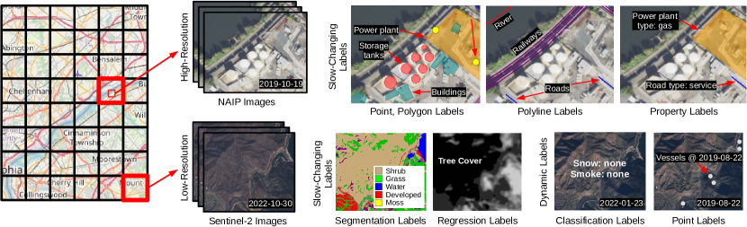
We present SatlasPretrain, a large-scale dataset for improving remote sensing image understanding models. Our goal with SatlasPretrain is to label everything that is visible in a satellite image. To this end, SatlasPretrain combines Sentinel-2 and NAIP images with 302M distinct labels under 137 diverse categories and 7 label types: the label types are points like wind turbines and water towers; polygons like buildings and airports; polylines like roads and rivers; segmentation and regression labels like land cover categories and bathymetry (water depth); properties of objects like the rotor diameter of a wind turbine; and patch classification labels like the presence of smoke in an image. Figure 1 demonstrates the wide range of categories in SatlasPretrain, along with the diverse applications that they serve.

We find that the huge scale of SatlasPretrain enables pre-training to substantially improve downstream performance. We compare SatlasPretrain pre-training against pre-training on other datasets as well as self-supervised learning methods, and find that it improves average performance across seven downstream tasks by 18% over ImageNet and 6% over the next best baseline. These results show that SatlasPretrain can readily improve accuracy on the numerous niche remote sensing tasks that require costly expert annotation.

Additionally, we believe that SatlasPretrain will encourage work on computer vision methods that tackle the unique research challenges in the remote sensing domain. Compared to general-purpose computer vision methods, remote sensing models require specialized techniques such as accounting for long-range spatial context, synthesizing information across images over time captured by diverse sensors like multispectral images and synthetic aperture radar (SAR), and predicting objects that vary widely in size, from forests spanning many km² to street lamps. We evaluate eight computer vision baselines on SatlasPretrain and find that no single existing method supports all the SatlasPretrain label types; instead, each baseline can only predict a subset of categories. Thus, inspired by recent work that integrate task-specific output heads [21, 35, 29, 36], we develop a unified model called SatlasNet that incorporates seven such heads so that it can learn from every category in the dataset. Compared to training separately on each label type, we find that jointly training SatlasNet on all categories and then fine-tuning on each label type improves average performance by 7.1%, showing that SatlasNet is able to leverage transfer learning opportunities between label types.

In summary, our contributions are:

1. SatlasPretrain, a large-scale remote sensing dataset with 137 categories under seven label types.

2. Demonstrating that pre-training on SatlasPretrain improves average performance on seven downstream datasets by 6%.

3. SatlasNet, a unified model that supports predictions for all label types in SatlasPretrain.

We have released the dataset and code at https://satlas-pretrain.allen.ai/. We have also released model weights pre-trained on SatlasPretrain  which can be fine-tuned for downstream tasks.

2 Related Work

Large-Scale Remote Sensing Datasets. Several general-purpose remote sensing computer vision datasets have been released. Many of these focus on scene and patch classification: the UC Merced Land Use (UCM) [57] and BigEarthNet [51] datasets involve land cover classification with 21 and 43 categories respectively, while the AID [56], Million-AID [39], RESISC45 [19], and Functional Map of the World (FMoW) [22] datasets additionally include categories corresponding to manmade structures such as bridges and railway stations, with up to 63 categories. A few datasets focus on tasks other than scene classification. DOTA [55] involves detecting objects in 18 categories ranging from helicopter to roundabout. iSAID [58] involves instance segmentation for 15 categories.

	Types	Classes	Labels	Pixels	km2
SatlasPretrain	7	137	302222K	17003B	21320K
UCM [57]	1	21	2K	1B	1K
BigEarthNet [51]	1	43	1750K	9B	850K
AID [56]	1	30	10K	4B	14K
Million-AID [39]	1	51	37K	4B	18K
RESISC45 [19]	1	45	32K	2B	10K
FMoW [22]	1	63	417K	437B	1748K
DOTA [55]	1	19	99K	9B	38K
iSAID [58]	1	15	355K	9B	38K

Table 1: Comparison of SatlasPretrain against existing remote sensing datasets (K=thousands, B=billions). Types is number of label types and km² is area covered.

All of these datasets involve making predictions for a single label type, and most involve doing so from a single image. Thus, they are limited in three ways: the number of object categories, the diversity of labels, and the opportunities for approaches to learn to synthesize features across image time series. In contrast, SatlasPretrain incorporates 137 categories under seven label types (see full comparison in Table 1), and provides image time series that methods can leverage to improve prediction accuracy.

A few domain-specific datasets extend beyond these limitations. xView3 [42] involves predicting vessel positions (object detection) and attributes of those vessels such as vessel type and length (per-object classification and regression) in SAR images. PASTIS-R [28] involves panoptic segmentation of crop types in crop fields using a time series of SAR and optical satellite images captured by the Sentinel-1 and Sentinel-2 constellations. IEEE Data Fusion datasets incorporate various aerial and satellite images for tasks like land cover segmentation [48].

Self-Supervised and Multi-Task Learning for Remote Sensing. Similar to our work, these approaches share the goal of improving accuracy on downstream applications with few labels. Several methods [40, 7, 50, 49, 54, 11] incorporate temporal augmentations into a contrastive learning framework, where images of the same location captured at different times are encouraged to have closer representations than images of different locations. They show that the model improves downstream performance by learning invariance to transient differences between images of the same location, such as different lighting and nadir angle conditions as well as seasonal changes. GPNA proposes combining self-supervised learning with supervised training on diverse tasks [45].

3 SatlasPretrain

Figure 2: Overview of the SatlasPretrain dataset. SatlasPretrain consists of image time series and labels for 856K Web-Mercator tiles at zoom 13 (left). There are two image modes on which methods are trained and evaluated independently: high-resolution NAIP images (top) and low-resolution Sentinel-2 images (bottom). Labels may be slow-changing (corresponding to the most recent image at a tile) or dynamic (referencing a specific image and time).

We present SatlasPretrain, a very-large-scale dataset for remote sensing image understanding that improves on existing remote sensing datasets in three key ways:

1. Scale: SatlasPretrain contains 40x more image pixels and 150x more labels than the largest existing dataset.

2. Label diversity: Existing datasets in Table 1 have unimodal labels, e.g. only classification. SatlasPretrain labels span seven label types; furthermore, they comprise 137 categories, 2x more than the largest existing dataset.

3. Spatio-temporal images and labels: Rather than being tied to individual remote sensing images, our labels are associated with geographic coordinates (i.e., longitude-latitude positions) and time ranges. This enables methods to make predictions from multiple images across time, as well as leverage long-range spatial context from neighboring images. These features present new research challenges that, if solved, can greatly improve model performance.

We first provide an overview of the structure of SatlasPretrain and detail the imagery that it contains below. We then describe the labels and how they were collected.

3.1 Structure and Imagery

Figure 3: Geographic coverage of SatlasPretrain, with bright pixels indicating locations covered by images and labels in the dataset. SatlasPretrain spans all continents except Antarctica.

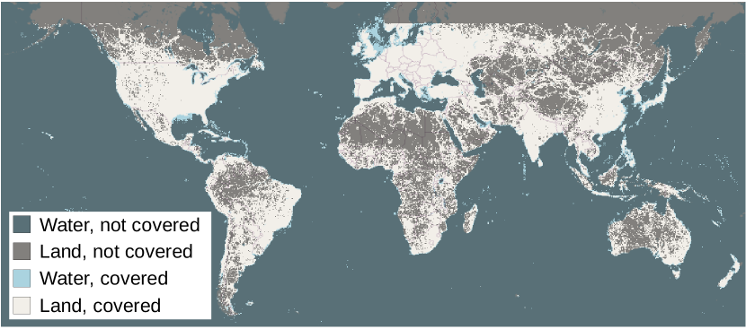
SatlasPretrain consists of 856K tiles. These tiles correspond to Web-Mercator tiles at zoom level 13, i.e., the world is projected to a 2D plane and divided into a $2^{13}\times 2^{13}$ grid, with each tile corresponding to a grid cell. Thus, each SatlasPretrain tile covers a disjoint spatial region spanning up to 25 km². At each tile, SatlasPretrain includes (1) a time series of remote sensing images of the tile; and (2) labels drawn from the 137 SatlasPretrain categories. Figure 2 summarizes the dataset, and Figure 3 shows its global geographic coverage.

Existing datasets typically use either high-resolution imagery (0.5–2 m/pixel) [19, 39, 22, 58] or low-resolution imagery (10 m/pixel) [51, 27]. Although high-resolution imagery enables higher prediction accuracy, low-resolution imagery is often employed in practical applications since it is available more frequently (weekly vs yearly) and broadly (globally vs in limited countries). Thus, in SatlasPretrain, we incorporate both low- and high-resolution images, which we will refer to as image modes. We define separate train and test splits for each image mode, and compare methods over each mode independently.

In all 856K tiles (828K train and 28K test), we provide low-resolution 512x512 images. Specifically, we include 8–12 Sentinel-2 images captured during 2022; this enables methods to leverage multiple spatially aligned images of a location to improve prediction accuracy. We also include historical 2016–2021 images that are relevant for dynamic labels like floods and ship positions. Sentinel-2 captures 10 m/pixel multispectral images; the European Space Agency (ESA) releases these images openly. Some categories are not visible in the low-resolution images, so for this mode we only evaluate methods on 122 of 137 categories.

In 46K tiles (45.5K train and 512 test), we provide high-resolution 8192x8192 images. We include 3–5 public domain 1 m/pixel aerial images from the US National Agriculture Imagery Program (NAIP) between 2011–2020. These images are only available in the US, so train and test tiles for the high-resolution mode are restricted to the US.

We download the images from ESA and USGS, and use GDAL [6] to process the images into Web-Mercator tiles.

The structure of SatlasPretrain enables methods to leverage both spatial and temporal context. Methods can make use of long-range spatial context from many neighboring tiles to improve the accuracy of predictions at a tile. Similarly, methods can learn to synthesize features across the image time series that we include at each tile in the dataset to improve prediction accuracy; for example, when predicting the crop type grown at a crop field, observations of the crop field at different stages of the agricultural cycle can provide different clues about the type of crop grown there. In contrast, existing datasets (including all but FMoW in Table 1) typically associate each label with a single image, and require methods to predict the label with that one image only.

3.2 Labels

SatlasPretrain labels span 137 categories, with seven label types (see examples in Figure 2):

1. Semantic segmentation—e.g., predicting per-pixel land cover (water vs forest vs developed vs etc.).

2. Regression—e.g., predicting per-pixel bathymetry (water depth) or percent tree cover.

3. Points (object detection)—e.g., predicting wind turbines, oil wells, and vessels.

4. Polygons (instance segmentation)—e.g., predicting buildings, dams, and aquafarms.

5. Polylines—e.g., predicting roads, rivers, and railways.

6. Properties of points, polygons, and polylines—e.g., the rotor diameter of a wind turbine.

7. Classification—e.g., whether an image exhibits negligible, low, or high wildfire smoke density.

Most categories represent slow-changing objects like roads or wind turbines. During dataset creation, we aim for labels under these categories to correspond to the most recent image available at each tile. Thus, during inference, if these objects change over the image time series available at a tile, the model predictions should reflect the last image in the time series. A few categories represent dynamic objects like vessels and floods. For labels in these categories, in addition to specifying the object position, the label specifies the timestamp of the image that it corresponds to. During inference, for dynamic categories, the model should make a separate set of predictions for each image in the time series.

We derive SatlasPretrain labels from seven sources: new annotation by domain experts, new annotation by Amazon Mechanical Turk (AMT) workers, and processing five existing datasets—OpenStreetMap [30], NOAA lidar scans, WorldCover [53], Microsoft Buildings [3], and C2S [5].

Each category is annotated (valid) in only a subset of tiles. Thus, in some tiles, a given category may be invalid, meaning that there is no ground truth for the category in that tile. In other tiles, a category may be valid but have zero labels, meaning that there are no instances of that category in the tile. In supplementary Section A.1, for each category, we detail the number of tiles where the category is valid, the number of tiles where the category has at least one label, and the number of labels under that category; we also detail the category’s label type and data source.

Labels in SatlasPretrain are relevant to numerous planet and environmental monitoring applications, which we discuss in supplementary Section A.2.

We summarize the data collection process for each of the data sources below.

Expert Annotation. Two domain experts annotated 12 categories: off-shore wind turbines, off-shore platforms, vessels, 6 tree cover categories (e.g. low vs high), and 3 snow presence categories (none, partial, or full). To facilitate this process, we built a dedicated annotation tool called Siv that is customizable for individual categories. For example, when annotating marine objects, we found that displaying images of the same marine location at different times was crucial for accurately distinguishing vessels from fixed infrastructure (generally, a vessel will only appear in one of the images, while wind turbines and platforms appear in all images); thus, for these categories, we ensured the domain experts could press the arrow keys in Siv to toggle between different spatially aligned images of the same tile. Similarly, for tree cover, we found that consulting external sources like Google Maps and OpenStreetMap helped improve accuracy in cases where tree cover was not clear in NAIP or Sentinel-2 images; thus, when annotating tree cover, we included links in Siv to these external sources.

AMT. AMT workers annotated 9 categories: coastal land, coastal water, fire retardant drops, areas burned by wildfires, airplanes, rooftop solar panels, and 3 smoke presence categories (none, low, or high). We reused the Siv annotation tool for AMT annotation, incorporating additional per-category customizations as needed (which we detail in supplementary Section A.3.1).

To maximize annotation quality, for each category, we first selected AMT workers through a qualification task: domain experts annotated between 100–400 tiles, and we asked each candidate AMT worker to annotate the same tiles; we only asked workers whose labels corresponded closely with expert labels to continue with further annotation. We also conducted majority voting over multiple workers; we decided the number of workers needed per tile on a per-category basis (see Section A.3.2), by first having one worker annotate each tile, and then analyzing the label quality. For example, we found that airplanes were unambiguous enough that a single worker sufficed, while we had three workers label each tile for areas burned by wildfires.

Figure 4: Model architecture of SatlasNet. A separate head is used to predict outputs for each label type. We visualize example outputs from two such heads (segmentation and polygon).

OpenStreetMap (OSM). OSM is a collaborative map dataset built through edits made by contributing users. Objects in OSM span a wide range of categories, from roads to power substations. We obtained OSM data as an OSM PBF file on 9 July 2022 from Geofabrik, and processed it using the Go osmpbf library to extract 101 categories.

Recall is a key issue for labels derived from OSM. From initial qualitative analysis, we consistently observed that OSM objects have high precision but variable recall: the vast majority of objects were correct, but for some categories, many objects were visible in satellite imagery but not mapped in OSM. To mitigate this issue, we employed heuristics to automatically prune tiles that most likely had low recall, based on the number of labels and distinct categories in the tile. For instance, we found that tiles with many roads but no buildings were likely to have missing objects in other categories like silo or water tower. We detail these heuristics in supplementary Section A.4.

We found that these heuristics were sufficient to yield high-quality labels for most categories. However, we identified 13 remaining low-recall categories, including gas stations, helipads, and oil wells. From an analysis of 1300 tiles, we determined that recall was still at least 80% for these categories, which we deemed sufficient for the training set: there are methods for learning from sparse labels, and large-scale training on noisy labels has produced models like CLIP that deliver state-of-the-art performance. However, we deemed that these 13 categories did not have sufficient recall for the test set. Thus, to ensure a highly accurate test set, for each of these 13 categories, we trained an initial model on OSM labels and tuned its confidence threshold for high-recall low-precision detection; we then hand-labeled its predictions to add missing labels to the test set. In Section A.4, we detail these categories and the number of missing labels identified in the test set.

NOAA Lidar Scans. NOAA coastal topobathy maps derived from lidar scans contain elevation data for land and depth data for water. We download 5,868 such maps from various NOAA surveys, and process them to derive per-pixel depth and elevation labels for 5,123 SatlasPretrain tiles.

WorldCover. WorldCover [53] is a global land cover map developed by the European Space Agency. We process the map to derive 11 land cover and land use categories, ranging from barren land to developed areas.

Microsoft Buildings. We process 70 GeoJSON files from various Microsoft Buildings datasets [3] to derive building polygons in SatlasPretrain. The data is released under ODbL.

C2S. C2S [5] consists of flood and cloud labels in Sentinel-2 images, released under CC-BY-4.0. We warp the labels to Web-Mercator and include them in SatlasPretrain. We also download and process the Sentinel-2 images that correspond exactly to the ones used in C2S, so that they share the same processing as other Sentinel-2 images in SatlasPretrain.

Balancing the scale of labels with label quality was a key consideration in managing new annotation and selecting existing data sources to process. As we developed the dataset, we conducted iterative analyses to evaluate the precision and recall of labels that we collected, and used this information to improve later annotation and refine data source processing. In supplementary Section A.5, we include an analysis of incorrect and missing labels under every category in the final dataset; we find that 116/137 categories have >99% precision, 15 have 95-99% precision, 4 have 90-95% precision, and 2 have 80-90% precision.

4 SatlasNet

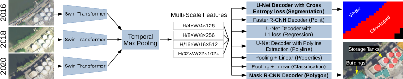
Off-the-shelf computer vision models cannot handle all the label types in SatlasPretrain, e.g., while Mask2Former [18] can simultaneously perform semantic and instance segmentation, it is not designed to predict properties of polygons or classify images. This prevents these models from leveraging the full set of transfer learning opportunities present in SatlasPretrain; for example, detecting building polygons is likely useful for segmenting images for land cover and land use, since land use includes a human-developed category. We develop a unified model, SatlasNet, that is capable of learning from all seven label types.

Figure 4 shows a schematic of our model. SatlasNet is inspired by recent work that employ task-specific output heads [21, 35, 29], as well as methods that synthesize features across remote sensing image time series [22, 27]. It inputs a time series of spatially aligned images, and processes each image (which may contain more than three bands) through a Swin Transformer [38] backbone (Swin-Base), which outputs feature maps for each image at four scales. We apply max temporal pooling at each scale to derive one set of multi-scale features. We pass the features to seven output heads (one for each label type) to compute outputs. For polylines, while specialized polyline extraction architectures have been shown to improve accuracy [10, 33, 52], we opt to employ the simpler segmentation approach [60] where we apply a UNet head to segment images for polyline categories, and post-process the segmentation probabilities with binary thresholding, morphological thinning, and line following and simplification [20] to extract polylines.

	High-Resolution NAIP Images						Low-Resolution Sentinel-2 Images
Method	Seg $\uparrow$	Reg $\downarrow$	Pt $\uparrow$	Pgon $\uparrow$	Pline $\uparrow$	Prop $\uparrow$	Seg $\uparrow$	Reg $\downarrow$	Pt $\uparrow$	Pgon $\uparrow$	Pline $\uparrow$	Prop $\uparrow$	Cls $\uparrow$
PSPNet (ResNext-101) [59]	77.8	15.0	-	-	53.2	-	62.1	16.2	-	-	30.7	-	-
LinkNet (ResNext-101) [15]	77.3	12.9	-	-	61.0	-	61.1	14.1	-	-	41.4	-	-
DeepLabv3 (ResNext-101) [16]	80.1	10.6	-	-	59.8	-	61.8	13.9	-	-	44.7	-	-
ResNet-50 [32]	-	-	-	-	-	87.6	-	-	-	-	-	70.3	97
ViT-Large [26]	-	-	-	-	-	78.1	-	-	-	-	-	66.9	99
Swin-Base [38]	-	-	-	-	-	87.1	-	-	-	-	-	69.4	99
Mask R-CNN (ResNet-50) [31]	-	-	27.6	30.4	-	-	-	-	22.0	12.3	-	-	-
Mask R-CNN (Swin-Base) [31]	-	-	30.4	31.5	-	-	-	-	25.6	15.2	-	-	-
ISTR [34]	-	-	2.0	4.9	-	-	-	-	1.2	1.4	-	-	-
SatlasNet (single-image, per-type)	79.4	8.3	28.0	30.4	61.5	86.6	64.8	9.3	25.7	14.8	42.5	67.5	99
SatlasNet (single-image, joint)	74.5	7.4	28.0	31.1	60.9	87.3	55.8	10.6	22.0	10.3	45.5	73.8	99
SatlasNet (single-image, fine-tuned)	79.8	7.2	32.3	33.0	62.4	89.5	65.3	9.0	27.4	16.3	45.9	80.0	99
SatlasNet (multi-image, per-type)	79.4	8.2	25.8	27.5	59.2	77.3	67.2	10.5	31.9	19.0	48.1	67.1	99
SatlasNet (multi-image, joint)	79.2	7.8	31.2	33.8	53.6	87.8	66.7	8.5	31.5	19.5	41.9	78.8	99
SatlasNet (multi-image, fine-tuned)	81.0	7.6	33.2	34.1	61.1	89.2	69.7	7.8	32.0	20.2	50.4	80.0	99

Table 2: Results on the SatlasPretrain test set for the high- and low-resolution image modes. We break down results by label type: segmentation (Seg), regression (Reg), points (Pt), polygons (Pgon), polylines (Pline), properties (Prop), and classification (Cls). We show absolute error for Reg (lower is better), and accuracy for the others (higher is better).

5 Evaluation

We first evaluate our method and eight classification, semantic segmentation, and instance segmentation baselines on the SatlasPretrain test split in Section 5.1. We then evaluate performance on seven downstream tasks in Section 5.2, comparing pre-training on SatlasPretrain to pre-training on other remote sensing datasets, as well as self-supervised learning techniques specialized for remote sensing.

5.1 Results on SatlasPretrain

Methods. We compare SatlasNet against eight baselines on SatlasPretrain. We select baselines that are either standard models or models that provide state-of-the-art performance for subsets of label types in SatlasPretrain. None of the baselines are able to handle all seven SatlasPretrain label types. For property prediction and classification, we compare ResNet [32], ViT [26], and Swin Transformer [38]. For segmentation, regression, and polylines, we compare PSPNet [59], LinkNet [15], and DeepLabv3 [16]. For points and polygons, we compare Mask R-CNN [31] and ISTR [34].

We train three variants of SatlasNet:

• Per-type: train separately on each label type.

• Joint: jointly train across all categories.

• Fine-tuned: fine-tune the jointly trained parameters on each label type.

All baselines are fine-tuned on each label type (after joint training on the subset of label types they can handle), which provides the highest performance.

For each SatlasNet variant, we also evaluate in single-image and multi-image modes. For all baselines and single-image SatlasNet, we sample training examples by either (a) sampling a tile, and pairing the most recent image at the tile with slow-changing labels (with dynamic and other invalid categories masked); or (b) sampling a tile and image, and pairing the image with corresponding dynamic labels. For multi-image SatlasNet, we provide as input a time series of eight Sentinel-2 images for low-resolution mode or four NAIP images for high-resolution mode; for slow-changing labels, the images are ordered by timestamp, but for dynamic labels, we always order the sampled image at the end of the time series input. In all cases, we sample examples based on the maximum inverse frequency of categories appearing in the example. We use RGB bands only here, but include results for single-image SatlasNet with nine Sentinel-2 bands in supplementary Section C.

Across all methods, we input 512x512 images during both training and inference; for high-resolution inference, since images covering the tile are 8K by 8K, we independently process 256 512x512 windows and merge the model outputs. We employ random cropping, horizontal and vertical flipping, and random resizing augmentations during training. We initialize models with ImageNet-pretrained weights. We use the Adam optimizer, and initialize the learning rate to $10^{-4}$, decaying via halving down to $10^{-6}$ upon plateaus in the training loss. We train with a batch size of 32 for 100K batches.

Metrics. We use standard metrics for each label type: accuracy for classification, F1 score for segmentation, mean absolute error for regression, mAP accuracy for points and polygons, and GEO accuracy [14] for polylines. We compute metrics per-category, and report the average across categories under each label type.

Figure 5: Qualitative results on SatlasPretrain. Rightmost: a failure case where SatlasNet detects only 1/5 oil wells.

	UCM		RESISC45		AID		FMoW		Mass Roads		Mass Buildings		Airbus Ships		Average
Method	50	All	50	All	50	All	50	All	50	All	50	All	50	All	50	All
Random Initialization	0.26	0.86	0.15	0.77	0.18	0.68	0.03	0.17	0.69	0.80	0.68	0.77	0.31	0.53	0.33	0.65
ImageNet [25]	0.35	0.92	0.17	0.95	0.20	0.81	0.03	0.21	0.77	0.85	0.78	0.83	0.37	0.65	0.38	0.75
BigEarthNet [51]	0.35	0.95	0.20	0.94	0.23	0.78	0.03	0.27	0.78	0.85	0.81	0.85	0.40	0.68	0.40	0.76
MillionAID [39]	0.72	0.97	0.30	0.96	0.30	0.82	0.04	0.35	0.78	0.84	0.82	0.85	0.46	0.67	0.49	0.78
DOTA [55]	0.56	0.99	0.28	0.95	0.33	0.83	0.03	0.30	0.82	0.86	0.84	0.87	0.62	0.75	0.50	0.79
iSAID [58]	0.60	0.97	0.29	0.97	0.34	0.86	0.04	0.30	0.82	0.86	0.84	0.86	0.55	0.73	0.50	0.79
MoCo [17]	0.14	0.14	0.07	0.09	0.05	0.12	0.02	0.03	0.56	0.69	0.62	0.63	0.01	0.21	0.21	0.27
SeCo [40]	0.48	0.95	0.20	0.90	0.27	0.74	0.03	0.26	0.70	0.81	0.71	0.77	0.27	0.54	0.38	0.71
SatlasPretrain	0.83	0.99	0.36	0.98	0.42	0.88	0.06	0.44	0.82	0.87	0.87	0.88	0.56	0.80	0.56	0.83

Table 3: Results on seven downstream tasks when fine-tuned with 50 examples (50) or the entire downstream dataset (All). Accuracy is reported for UCM, RESISC45, and AID while F1 Score is reported for FMoW, Mass Roads, Mass Buildings, and Airbus Ships. SatlasPretrain pre-training improves average accuracy across the tasks by 6% over the next best baseline.

Results. We show results on SatlasPretrain in Table 2. Across the seven label types, single-image SatlasNet matches or surpasses the performance of state-of-the-art, purpose-built baselines when trained per-type, validating its effectiveness as a unified model that can predict diverse remote sensing labels. Jointly training one set of SatlasNet parameters for all categories reduces average performance on several label types, but SatlasNet remains competitive in most cases; this training mode provides large efficiency gains since the backbone features need only be computed once for each image during inference, rather than once per label type. When fine-tuning SatlasNet on each label type using the parameters derived from joint training, it provides an average 7.1% relative improvement across the label types and image modes over per-type training. This supports our hypothesis that there are transfer learning opportunities between the label types, validating the utility of a unified model for improving performance. Multi-image SatlasNet provides another 5.6% relative improvement in average performance, showing that it is able to effectively synthesize information across image time series to produce better predictions; nevertheless, we believe that there is substantial room for further improvement in methods for processing remote sensing image time series.

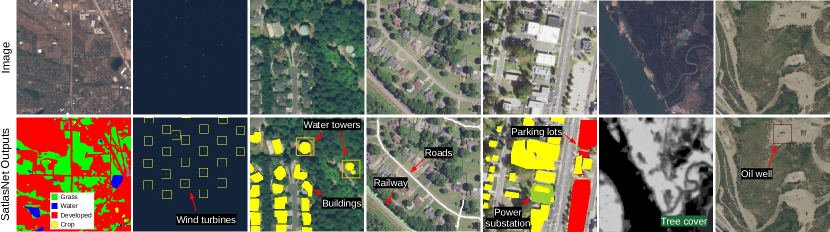
We show qualitative results in Figure 5, with additional examples in supplementary Section E. We achieve high accuracy on several categories, such as wind turbines and water towers. However, for oil wells, one well is detected but several others are not. Similarly, for polyline features like roads and railways, the model produces short noisy segments, despite ample training data for these categories; we believe that incorporating and improving models that are tailored for specialized output types like polylines [33, 52] has the potential to improve accuracy.

5.2 Downstream Performance

We now evaluate accuracy on seven downstream tasks when pre-training on SatlasPretrain compared to pre-training on four existing remote sensing datasets, as well as two self-supervised learning methods. For each downstream task, we evaluate accuracy when training on just 50 examples and when training on the whole dataset, to focus on the challenge of improving performance on niche remote sensing applications that require expert annotation and thus have few labeled examples.

Methods. We compare pre-training on high-resolution images in SatlasPretrain to pre-training on four existing remote sensing datasets: BigEarthNet [51], Million-AID [39], DOTA [55], and iSAID [58]. We use SatlasNet in all cases, fine-tuning the pre-trained Swin backbone on each downstream dataset.

We also compare two self-supervised learning methods, Momentum Contrast v2 (MoCo) [17] and Seasonal Contrast (SeCo) [40]. The latter is a specialized method for remote sensing that leverages multiple image captures of the same location to learn invariance to seasonal changes. For MoCo, we use our SatlasNet model and train on SatlasPretrain images. For SeCo, we evaluate their original model trained on their dataset. We fine-tune the weights learned through self-supervision on the downstream tasks. We provide results for additional variants in supplementary Section B.3.

We fine-tune both the pre-training and self-supervised learning methods by first freezing the backbone and only training the prediction head for 32K examples, and then fine-tuning the entire model. We provide additional experiment details in supplementary Section B.1.

Downstream Datasets. The downstream tasks consist of four existing large-scale remote sensing datasets that involve classification with between 21 and 63 categories: UCM [57], AID [56], RESISC45 [19], and FMoW [22]. The other three are the Massachusetts Buildings and Massachusetts Roads datasets [41], which involve semantic segmentation, and the Airbus Ships [2] dataset, which involves instance segmentation.

Results. Table 3 shows downstream performance with varying training set sizes. SatlasPretrain consistently outperforms the baselines: when training on 50 examples, we improve average accuracy across the tasks by 18% over ImageNet pre-training, and by 6% over the next best baseline. The state-of-the-art performance achieved across such a wide range of downstream tasks clearly demonstrates the generalizability of the representations derived from SatlasPretrain pre-training, and the potential of SatlasPretrain to improve performance on the numerous niche remote sensing applications. We include results with more varying training examples in supplementary B.2.

6 Use in AI-Generated Geospatial Data

We have deployed SatlasPretrain to develop high-accuracy models for Satlas (https://satlas.allen.ai/), a platform for global geospatial data generated by AI from satellite imagery. Timely geospatial data, like the positions of wind turbines and solar farms, is critical for informing decisions in emissions reduction, disaster relief, urban planning, etc. However, high-quality global geospatial data products can be hard to find because manual curation is often cost-prohibitive. Satlas instead applies models fine-tuned for tasks like wind turbine detection to automatically extract geospatial data from satellite imagery on a monthly basis. Satlas currently consists of four geospatial data products: wind turbines, solar farms, offshore platforms, and tree cover.

7 Conclusion

By improving on existing datasets in both scale and label diversity, SatlasPretrain serves as an effective very-large-scale dataset for remote sensing methods. Pre-training on SatlasPretrain increases average downstream accuracy by 18% over ImageNet and 6% over existing remote sensing datasets, indicating that it can readily be applied to the long tail of remote sensing tasks that have few labeled examples. We have already leveraged models pre-trained on SatlasPretrain to accurately detect wind turbines, solar farms, offshore platforms, and tree cover in the Satlas platform at https://satlas.allen.ai/.

Appendix A Supplementary Material

The supplementary material can be accessed from https://github.com/allenai/satlas/blob/main/SatlasPretrain.md.

References

- [1] The machine vision challenge to better analyze satellite images of Earth. MIT Technology Review.
- [2] Airbus ship detection challenge. https://www.kaggle.com/c/airbus-ship-detection, 2018. Airbus.
- [3] Microsoft Building Footprints Datasets, 2021. Microsoft.
- [4] Copernicus Sentinel Missions. https://sentinel.esa.int/web/sentinel/home, 2022. European Space Agency.
- [5] A global flood events and cloud cover dataset (version 1.0), 2022. Cloud to Street, Microsoft, Radiant Earth Foundation.
- [6] GDAL, 2023. Open Source Geospatial Foundation.
- [7] Peri Akiva, Matthew Purri, and Matthew Leotta. Self-supervised Material and Texture Representation Learning for Remote Sensing Tasks. In Proceedings of the IEEE/CVF Conference on Computer Vision and Pattern Recognition (CVPR), pages 8203–8215, 2022.
- [8] Robert S Allison, Joshua M Johnston, Gregory Craig, and Sion Jennings. Airborne Optical and Thermal Remote Sensing for Wildfire Detection and Monitoring. Sensors, 16(8):1310, 2016.
- [9] Manuela Andreoni, Blacki Migliozzi, Pablo Robles, and Denise Lu. The Illegal Airstrips Bringing Toxic Mining to Brazil’s Indigenous Land. The New York Times.
- [10] Favyen Bastani, Songtao He, Sofiane Abbar, Mohammad Alizadeh, Hari Balakrishnan, Sanjay Chawla, Sam Madden, and David DeWitt. RoadTracer: Automatic Extraction of Road Networks from Aerial Images. In Proceedings of the IEEE/CVF Conference on Computer Vision and Pattern Recognition (CVPR), pages 4720–4728, 2018.
- [11] Favyen Bastani, Songtao He, Satvat Jagwani, Mohammad Alizadeh, Hari Balakrishnan, Sanjay Chawla, Sam Madden, and Mohammad Amin Sadeghi. Updating Street Maps using Changes Detected in Satellite Imagery. In Proceedings of the 29th International Conference on Advances in Geographic Information Systems, pages 53–56, 2021.
- [12] Favyen Bastani and Samuel Madden. Beyond Road Extraction: A Dataset for Map Update using Aerial Images. In Proceedings of the IEEE/CVF International Conference on Computer Vision (ICCV), pages 11905–11914, 2021.
- [13] Anil Batra, Suriya Singh, Guan Pang, Saikat Basu, CV Jawahar, and Manohar Paluri. Improved Road Connectivity by Joint Learning of Orientation and Segmentation. In Proceedings of the IEEE/CVF Conference on Computer Vision and Pattern Recognition (CVPR), pages 10385–10393, 2019.
- [14] James Biagioni and Jakob Eriksson. Map Inference in the Face of Noise and Disparity. In Proceedings of the 20th International Conference on Advances in Geographic Information Systems, pages 79–88, 2012.
- [15] Abhishek Chaurasia and Eugenio Culurciello. LinkNet: Exploiting encoder representations for efficient semantic segmentation. IEEE Visual Communications and Image Processing (VCIP), pages 1–4, 2017.
- [16] Liang-Chieh Chen, George Papandreou, Florian Schroff, and Hartwig Adam. Rethinking Atrous Convolution for Semantic Image Segmentation. ArXiv, abs/1706.05587, 2017.
- [17] Xinlei Chen, Haoqi Fan, Ross Girshick, and Kaiming He. Improved Baselines with Momentum Contrastive Learning. arXiv preprint arXiv:2003.04297, 2020.
- [18] Bowen Cheng, Ishan Misra, Alexander G. Schwing, Alexander Kirillov, and Rohit Girdhar. Masked-attention Mask Transformer for Universal Image Segmentation. 2022.
- [19] Gong Cheng, Junwei Han, and Xiaoqiang Lu. Remote Sensing Image Scene Classification: Benchmark and State of the Art. In Proceedings of the IEEE, volume 105, pages 1865–1883, 2017.
- [20] Guangliang Cheng, Ying Wang, Shibiao Xu, Hongzhen Wang, Shiming Xiang, and Chunhong Pan. Automatic Road Detection and Centerline Extraction via Cascaded End-to-end Convolutional Neural Network. IEEE Transactions on Geoscience and Remote Sensing, 55(6):3322–3337, 2017.
- [21] Jaemin Cho, Jie Lei, Hao Tan, and Mohit Bansal. Unifying Vision-and-Language Tasks via Text Generation. In International Conference on Machine Learning, pages 1931–1942. PMLR, 2021.
- [22] Gordon Christie, Neil Fendley, James Wilson, and Ryan Mukherjee. Functional Map of the World. In Proceedings of the IEEE/CVF Conference on Computer Vision and Pattern Recognition (CVPR), 2018.
- [23] Annarita D’Addabbo, Alberto Refice, Guido Pasquariello, Francesco P Lovergine, Domenico Capolongo, and Salvatore Manfreda. A Bayesian Network for Flood Detection Combining SAR Imagery and Ancillary Data. IEEE Transactions on Geoscience and Remote Sensing, 54(6):3612–3625, 2016.
- [24] Ilke Demir, Krzysztof Koperski, David Lindenbaum, Guan Pang, Jing Huang, Saikat Basu, Forest Hughes, Devis Tuia, and Ramesh Raskar. DeepGlobe 2018: A Challenge to Parse the Earth through Satellite Images. In Proceedings of the IEEE/CVF Conference on Computer Vision and Pattern Recognition (CVPR) Workshops, pages 172–181, 2018.
- [25] J. Deng, W. Dong, R. Socher, L. J. Li, Kai Li, and Li Fei-Fei. ImageNet: A large-scale hierarchical image database. IEEE Conference on Computer Vision and Pattern Recognition (CVPR), 2009.
- [26] Alexey Dosovitskiy, Lucas Beyer, Alexander Kolesnikov, Dirk Weissenborn, Xiaohua Zhai, Thomas Unterthiner, Mostafa Dehghani, Matthias Minderer, Georg Heigold, Sylvain Gelly, Jakob Uszkoreit, and Neil Houlsby. An Image is Worth 16x16 Words: Transformers for Image Recognition at Scale. In International Conference on Learning Representations, 2021.
- [27] Vivien Sainte Fare Garnot and Loic Landrieu. Panoptic Segmentation of Satellite Image Time Series with Convolutional Temporal Attention Networks. In Proceedings of the IEEE/CVF International Conference on Computer Vision (ICCV), pages 4872–4881, 2021.
- [28] Vivien Sainte Fare Garnot, Loic Landrieu, and Nesrine Chehata. Multi-modal Temporal Attention Models for Crop Mapping from Satellite Time Series. ISPRS Journal of Photogrammetry and Remote Sensing, pages 294–305, 2022.
- [29] Tanmay Gupta, Amita Kamath, Aniruddha Kembhavi, and Derek Hoiem. Towards General Purpose Vision Systems: An End-to-End Task-Agnostic Vision-Language Architecture. In Proceedings of the IEEE/CVF Conference on Computer Vision and Pattern Recognition (CVPR), pages 16399–16409, 2022.
- [30] Mordechai Haklay and Patrick Weber. OpenStreetMap: User-Generated Street Maps. IEEE Pervasive computing, 7(4):12–18, 2008.
- [31] Kaiming He, Georgia Gkioxari, Piotr Dollár, and Ross Girshick. Mask r-cnn. In IEEE International Conference on Computer Vision (ICCV), pages 2980–2988, 2017.
- [32] Kaiming He, Xiangyu Zhang, Shaoqing Ren, and Jian Sun. Deep Residual Learning for Image Recognition. In Proceedings of the IEEE/CVF Conference on Computer Vision and Pattern Recognition (CVPR), pages 770–778, 2016.
- [33] Songtao He, Favyen Bastani, Satvat Jagwani, Mohammad Alizadeh, Hari Balakrishnan, Sanjay Chawla, Mohamed M Elshrif, Samuel Madden, and Mohammad Amin Sadeghi. Sat2Graph: Road Graph Extraction through Graph-Tensor Encoding. European Conference on Computer Vision, pages 51–67, 2020.
- [34] Jie Hu, Liujuan Cao, Yao Lu, Shengchuan Zhang, Yan Wang, Ke Li, Feiyue Huang, Ling Shao, and Rongrong Ji. ISTR: End-to-End Instance Segmentation with Transformers. ArXiv, abs/2105.00637, 2021.
- [35] Ronghang Hu and Amanpreet Singh. Unit: Multimodal Multitask Learning with a Unified Transformer. In Proceedings of the IEEE/CVF International Conference on Computer Vision (ICCV), pages 1439–1449, 2021.
- [36] Amita Kamath, Christopher Clark, Tanmay Gupta, Eric Kolve, Derek Hoiem, and Aniruddha Kembhavi. Webly Supervised Concept Expansion for General Purpose Vision Models. arXiv preprint arXiv:2202.02317, 2022.
- [37] Zuoyue Li, Jan Dirk Wegner, and Aurélien Lucchi. Topological Map Extraction from Overhead Images. In Proceedings of the IEEE/CVF International Conference on Computer Vision (ICCV), pages 1715–1724, 2019.
- [38] Z. Liu, Y. Lin, Y. Cao, H. Hu, Y. Wei, Z. Zhang, S. Lin, and B. Guo. Swin Transformer: Hierarchical Vision Transformer using Shifted Windows. In IEEE/CVF International Conference on Computer Vision (ICCV), pages 9992–10002, 2021.
- [39] Yang Long, Gui-Song Xia, Shengyang Li, Wen Yang, Michael Ying Yang, Xiao Xiang Zhu, Liangpei Zhang, and Deren Li. On Creating Benchmark Dataset for Aerial Image Interpretation: Reviews, Guidances, and Million-AID. IEEE Journal of Selected Topics in Applied Earth Observations and Remote Sensing, pages 4205–4230, 2021.
- [40] Oscar Manas, Alexandre Lacoste, Xavier Giro i Nieto, David Vazquez, and Pau Rodriguez. Seasonal Contrast: Unsupervised Pre-Training from Uncurated Remote Sensing Data. In Proceedings of the IEEE/CVF International Conference on Computer Vision (ICCV), 2021.
- [41] Volodymyr Mnih. Machine Learning for Aerial Image Labeling. PhD thesis, University of Toronto, 2013.
- [42] Fernando Paolo, Tsu ting Tim Lin, Ritwik Gupta, Bryce Goodman, Nirav Patel, Daniel Kuster, David Kroodsma, and Jared Dunnmon. xView3-SAR: Detecting Dark Fishing Activity Using Synthetic Aperture Radar Imagery. Neural Information Processing Systems, 2022.
- [43] Alec Radford, Jong Wook Kim, Chris Hallacy, Aditya Ramesh, Gabriel Goh, Sandhini Agarwal, Girish Sastry, Amanda Askell, Pamela Mishkin, Jack Clark, et al. Learning Transferable Visual Models from Natural Language Supervision. International Conference on Machine Learning, pages 8748–8763, 2021.
- [44] Sudha Radhika, Yukio Tamura, and Masahiro Matsui. Application of Remote Sensing Images for Natural Disaster Mitigation using Wavelet based Pattern Recognition Analysis. In 2016 IEEE International Geoscience and Remote Sensing Symposium (IGARSS), pages 84–87, 2016.
- [45] Nasim Rahaman, Martin Weiss, Frederik Träuble, Francesco Locatello, Alexandre Lacoste, Yoshua Bengio, Chris Pal, Li Erran Li, and Bernhard Schölkopf. A General Purpose Neural Architecture for Geospatial Systems. HADR Workshop at NeurIPS 2022, 2022.
- [46] Caleb Robinson, Le Hou, Kolya Malkin, Rachel Soobitsky, Jacob Czawlytko, Bistra Dilkina, and Nebojsa Jojic. Large Scale High-Resolution Land Cover Mapping with Multi-Resolution Data. In Proceedings of the IEEE/CVF Conference on Computer Vision and Pattern Recognition (CVPR), pages 12726–12735, 2019.
- [47] Caleb Robinson, Anthony Ortiz, Kolya Malkin, Blake Elias, Andi Peng, Dan Morris, Bistra Dilkina, and Nebojsa Jojic. Human-Machine Collaboration for Fast Land Cover Mapping. pages 2509–2517, 2020.
- [48] Ronny Hänsch; Claudio Persello; Gemine Vivone; Javiera Castillo Navarro; Alexandre Boulch; Sebastien Lefevre; Bertrand Le Saux. Data fusion contest 2022 (dfc2022), 2022.
- [49] Linus Scheibenreif, Joëlle Hanna, Michael Mommert, and Damian Borth. Self-Supervised Vision Transformers for Land-Cover Segmentation and Classification. In Proceedings of the IEEE/CVF Conference on Computer Vision and Pattern Recognition (CVPR), pages 1422–1431, 2022.
- [50] Linus Scheibenreif, Michael Mommert, and Damian Borth. Contrastive Self-Supervised Data Fusion for Satellite Imagery. ISPRS Annals of the Photogrammetry, Remote Sensing and Spatial Information Sciences, 3:705–711, 2022.
- [51] Gencer Sumbul, Marcela Charfuelan, Begum Demir, and Volker Markl. BigEarthNet: A Large-Scale Benchmark Archive for Remote Sensing Image Understanding. In International Geoscience and Remote Sensing Symposium (IGARSS), 2019.
- [52] Yong-Qiang Tan, Shang-Hua Gao, Xuan-Yi Li, Ming-Ming Cheng, and Bo Ren. VecRoad: Point-based Iterative Graph Exploration for Road Graphs Extraction. In Proceedings of the IEEE/CVF Conference on Computer Vision and Pattern Recognition (CVPR), pages 8910–8918, 2020.
- [53] Ruben Van De Kerchove, Daniele Zanaga, Wanda Keersmaecker, Niels Souverijns, Jan Wevers, Carsten Brockmann, Alex Grosu, Audrey Paccini, Oliver Cartus, Maurizio Santoro, et al. ESA WorldCover: Global land cover mapping at 10 m resolution for 2020 based on Sentinel-1 and 2 data. In AGU Fall Meeting Abstracts, volume 2021, pages GC45I–0915, 2021.
- [54] Yi Wang, Nassim Ait Ali Braham, Zhitong Xiong, Chenying Liu, Conrad M. Albrecht, and Xiao Xiang Zhu. SSL4EO-S12: A Large-Scale Multi-Modal, Multi-Temporal Dataset for Self-Supervised Learning in Earth Observation. ArXiv, abs/2211.07044, 2022.
- [55] Gui-Song Xia, Xiang Bai, Jian Ding, Zhen Zhu, Serge Belongie, Jiebo Luo, Mihai Datcu, Marcello Pelillo, and Liangpei Zhang. DOTA: A Large-scale Dataset for Object Detection in Aerial Images. In Proceedings of the IEEE/CVF Conference on Computer Vision and Pattern Recognition (CVPR), 2018.
- [56] Gui-Song Xia, Jingwen Hu, Fan Hu, Baoguang Shi, Xiang Bai, Yanfei Zhong, and Liangpei Zhang. AID: A Benchmark Dataset for Performance Evaluation of Aerial Scene Classification. IEEE Journal of Transactions on Geoscience and Remote Sensing, 55(7):3965–3981, 2017.
- [57] Yi Yang and Shawn Newsam. Bag-Of-Visual-Words and Spatial Extensions for Land-Use Classification. ACM Conference on Spatial Information (SIGSPATIAL), 2010.
- [58] Syed Waqas Zamir, Aditya Arora, Akshita Gupta, Salman Khan, Guolei Sun, Fahad Shahbaz Khan, Fan Zhu, Ling Shao, Gui-Song Xia, and Xiang Bai. iSAID: A Large-scale Dataset for Instance Segmentation in Aerial Images. In Proceedings of the IEEE/CVF Conference on Computer Vision and Pattern Recognition (CVPR) Workshops, 2019.
- [59] Hengshuang Zhao, Jianping Shi, Xiaojuan Qi, Xiaogang Wang, and Jiaya Jia. Pyramid Scene Parsing Network. In Proceedings of the IEEE/CVF Conference on Computer Vision and Pattern Recognition (CVPR), pages 6230–6239, 2017.
- [60] Lichen Zhou, Chuang Zhang, and Ming Wu. D-LinkNet: LinkNet with Pretrained Encoder and Dilated Convolution for High Resolution Satellite Imagery Road Extraction. In Proceedings of the IEEE/CVF Conference on Computer Vision and Pattern Recognition (CVPR) Workshops, pages 182–186, 2018.
- [61] Stefano Zorzi, Shabab Bazrafkan, Stefan Habenschuss, and Friedrich Fraundorfer. PolyWorld: Polygonal Building Extraction with Graph Neural Networks in Satellite Images. In Proceedings of the IEEE/CVF Conference on Computer Vision and Pattern Recognition (CVPR), pages 1848–1857, 2022.