A posteriori error bounds for the block-Lanczos method for matrix function approximation

Abstract

We extend the error bounds from [SIMAX, Vol. 43, Iss. 2, pp. 787-811 (2022)] for the Lanczos method for matrix function approximation to the block algorithm. Numerical experiments suggest that our bounds are fairly robust to changing block size and have the potential for use as a practical stopping criterion. Further experiments work towards a better understanding of how certain hyperparameters should be chosen in order to maximize the quality of the error bounds, even in the previously studied block size one case.

1 Introduction

Lanczos-based methods have proven to be among the most effective algorithms for approximating $f(\mathbf{H})\mathbf{v}$, where $f:\mathbb{R}\to\mathbb{R}$ is a scalar function, $\mathbf{H}$ is a $n\times n$ Hermitian matrix, and $\mathbf{v}$ is a vector. As a result, a number of analyses aim to provide a posteriori error bounds which may be used as practical stopping criteria [FS08a, FS09, ITS09, FKLR13, FGS14, FS15, CGMM22]. In particular, for a large class of functions, [CGMM22] shows a general approach to bounding the error for the approximation of the Lanczos function approximation algorithm (referred to as Lanczos-FA) to $f(\mathbf{H})\mathbf{v}$ in terms of the error of Lanczos-FA used to approximate a fixed linear system $(\mathbf{H}-w\mathbf{I})\mathbf{x}=\mathbf{v}$. In the case that $\mathbf{H}-w\mathbf{I}$ is positive definite, Lanczos-FA is mathematically equivalent to the well-known and optimal conjugate gradient algorithm [Gre97], and the error of this linear system can then be accurately estimated or bounded using existing techniques. In fact, the residual can always be used as an estimate for the error of the approximate solution to the system $(\mathbf{H}-w\mathbf{I})\mathbf{x}=\mathbf{v}$.

Often, one would like to approximate a sequence $f(\mathbf{H})\mathbf{v}_{1},\ldots,f(\mathbf{H})\mathbf{v}_{b}$ for some set of vectors $\{\mathbf{v}_{1},\ldots,\mathbf{v}_{b}\}$. Examples of applications in which such a situation arises include solving multiple systems of linear equations with varying right-hand sides, computing Lyapunov exponents for dynamical systems, low-rank and diagonal approximation of matrix functions, model order reduction, sampling Gaussian vectors, and studying the equilibrium thermodynamics of open quantum systems [DV95, ACSS12, BBJ15, FMR16, LM16, Bir18, SY20, chen_hallman_23, CC22]. While it is possible to apply the standard Lanczos-FA to each product independently, it is often more efficient to apply a blocked version of Lanczos-FA to approximate $f(\mathbf{H})\mathbf{V}$ directly, where $\mathbf{V}=[\mathbf{v}_{1},\ldots,\mathbf{v}_{b}]$ is a “block-vector” (i.e. a tall/skinny $n\times b$ matrix) [GU77, FLS17].

In this paper, we extend the bounds of [CGMM22] to the block-Lanczos-FA algorithm. In particular, we show that, for piece-wise analytic $f$, the error of the block-Lanczos-FA algorithm can be bounded by the product of (i) the error of the block-Lanczos-FA approximation to the block system $(\mathbf{H}-w\mathbf{I})\mathbf{X}=\mathbf{V}$ and (ii) a certain contour integral which can be approximated numerically from quantities made available by the block-Lanczos algorithm. As in [CGMM22], the bounds depend on the choice of $w$ as well as a certain contour of integration $\Gamma$.

Since bounds and stopping criteria for block-Lanczos-FA are less studied than for standard Lanczos-FA, we believe that the present work provides a useful tool for practitioners using the block algorithm. We include a number of numerical experiments exploring the impact of block size on our bounds, as well as experiments that provide further intuition as to how hyper-parameters such as $w$ and $\Gamma$ should be chosen. These experiments are relevant for the block size one case as well and serve as a step towards addressing some of the practical questions raised in [CGMM22].

1.1 Notation

We denote vectors with bold lowercase Roman letters and matrices with bold uppercase Roman letters. Constants are denoted with unbolded lowercase Roman letters. Throughout, $b$ is the block size of a matrix, $k$ is the number of iterations of the block-Lanczos algorithm, and $\mathbf{E}_{i}$ is defined as the $(kb)\times b$ block matrix whose $i$-th $b\times b$ block is the identity matrix. We write $\lambda_{\textup{min}}$ and $\lambda_{\textup{max}}$ for the smallest and largest eigenvalues of $\mathbf{H}$ respectively. The spectrum of a matrix $\mathbf{B}$ is denoted by $\Lambda(\mathbf{B})$.

We use the notation $\|\cdot\|_{2}$ and $\|\cdot\|_{\mathsf{F}}$ to respectively denote the two-norm and Frobenius norm of a vector or a matrix. We will use $\|\cdot\|=\|\cdot\|_{h(\mathbf{H})}$ to denote some fixed norm induced by a positive definite matrix $\mathbf{M}=h(\mathbf{H})$ by the relation $\|\mathbf{X}\|_{h(\mathbf{H})}=\|h(\mathbf{H})^{1/2}\mathbf{X}\|_{\mathsf{F}}$. In the case that $\mathbf{X}$ has a single column, this coincides with the standard definition of a matrix-induced norm. Note for any function $g$ and matrices $\mathbf{X},\mathbf{Y}$, such norms satisfy the inequality

$$\|g(\mathbf{H})\mathbf{X}\mathbf{Y}\| =\|h(\mathbf{H})^{1/2}g(\mathbf{H})\mathbf{X}\mathbf{Y}\|_{\mathsf{F}}\leq\|g(\mathbf{H})\|_{2}\|h(\mathbf{H})^{1/2}\mathbf{X}\mathbf{Y}\|_{\mathsf{F}}$$

$$\hskip 40.00006pt\leq\|g(\mathbf{H})\|_{2}\|h(\mathbf{H})^{1/2}\mathbf{X}\|_{\mathsf{F}}\|\mathbf{Y}\|_{2}=\|g(\mathbf{H})\|_{2}\|\mathbf{X}\|\|\mathbf{Y}\|_{2}.$$ (1)

1.2 The block-Lanczos method for matrix function approximation

Given a matrix $\mathbf{V}\in\mathbb{R}^{n\times b}$, the degree $j$ block-Krylov subspace is defined as

$$\mathcal{K}_{j+1}(\mathbf{H},\mathbf{V}):=\operatorname{span}\{\mathbf{V},\mathbf{H}\mathbf{V},\ldots,\mathbf{H}^{j}\mathbf{V}\}.$$

Here the span of a set of block vectors is interpreted as the span of the constituent columns. The block-Lanczos algorithm [Und75, GU77], which we described in Algorithm 1, computes matrices $\{\mathbf{Q}_{j}\}$, $j\leq k+1$ such that $\mathbf{Q}_{i}^{*}\mathbf{Q}_{j}=\mathbf{0}$ for all $i\neq j$ and $\mathbf{Q}_{i}^{*}\mathbf{Q}_{i}=\mathbf{I}$. Moreover, these matrices satisfy, for all $j\leq k+1$,

$$\operatorname{span}\{\mathbf{Q}_{1},\mathbf{Q}_{2},\ldots,\mathbf{Q}_{j}\}=\mathcal{K}_{j+1}(\mathbf{H},\mathbf{V}).$$

As a result, the block vectors $\{\mathbf{Q}_{j}\}$ satisfy a symmetric block-tridiagonal recurrence

$$\mathbf{H}\mathbf{Q}=\mathbf{Q}\mathbf{T}+\mathbf{Q}_{k+1}\mathbf{B}_{k}\mathbf{E}_{k}^{*}$$ (2)

where

$$\mathbf{T}=\begin{bmatrix}\mathbf{A}_{1}&\mathbf{B}_{1}^{*}\\ \mathbf{B}_{1}&\ddots&\ddots\\ &\ddots&\ddots&\mathbf{B}_{k-1}^{*}\\ &&\mathbf{B}_{k-1}&\mathbf{A}_{k}\end{bmatrix}, \mathbf{Q}=\begin{bmatrix}|&|&&|\\ \mathbf{Q}_{1}&\mathbf{Q}_{2}&\cdots&\mathbf{Q}_{k}\\ |&|&&|\end{bmatrix}$$

are block matrices of size $(bk)\times(bk)$ and $n\times(bk)$ respectively. The $b\times b$ diagonal blocks $\{\mathbf{A}_{i}\}$ and the $b\times b$ upper triangular off-diagonal blocks $\{\mathbf{B}_{i}\}$ are also generated by the block-Lanczos algorithm.

The output of the block-Lanczos algorithm can be used to approximate $f(\mathbf{H})\mathbf{V}$:

Definition 1.

The block-Lanczos method for matrix function approximation (block-Lanczos-FA) for $f(\mathbf{H})\mathbf{V}$ is defined as

$$\textup{{lan}}_{k}(f):=\mathbf{Q}f(\mathbf{T})\mathbf{E}_{1}\mathbf{B}_{0}.$$

In the case that $b=1$, the block-Lanczos-FA algorithm is the same as the well-known Lanczos-FA algorithm; see for instance [Saa92].

Algorithm 1 block-Lanczos algorithm

1:procedure block-Lanczos($\mathbf{H},\mathbf{V},k$)

2:     $\mathbf{Q}_{1},\mathbf{B}_{0}=\textsc{qr}(\mathbf{V})$,

3:     for $j=1,2,\ldots,k$ do

4:         $\mathbf{Z}=\mathbf{H}\mathbf{Q}_{j}-\mathbf{Q}_{j-1}\mathbf{B}_{j-1}^{*}$ $\triangleright$ if $j=1$, $\mathbf{Z}=\mathbf{H}\mathbf{Q}_{1}$

5:         $\mathbf{A}_{j}=\mathbf{Q}_{j}^{*}\mathbf{Z}$

6:         $\mathbf{Z}=\mathbf{Z}-\mathbf{Q}_{j}\mathbf{A}_{j}$

7:         optionally, reorthogonalize $\mathbf{Z}$ against $\mathbf{Q}_{0},\ldots,\mathbf{Q}_{j-1}$

8:         $\mathbf{Q}_{j+1},\mathbf{B}_{j}=\textsc{qr}(\mathbf{Z})$      

9:     return $\{\mathbf{Q}_{j}\},\{\mathbf{A}_{j}\},\{\mathbf{B}_{j}\}$

1.3 Past work and existing error bounds

It is straightforward to show that for any polynomial $p$ with $\deg(p)<k$, $p(\mathbf{H})\mathbf{V}=\textup{{lan}}_{k}(p)$. That is, block-Lanczos-FA applies low-degree polynomials exactly. Writing the smallest and largest eigenvalues of $\mathbf{H}$ as $\lambda_{\textup{min}}$ and $\lambda_{\textup{max}}$ respectively, the previous observation implies that block-Lanczos-FA satisfies the error bound:

$$\|f(\mathbf{H})\mathbf{V}-\textup{{lan}}_{k}(f)\|_{2}\leq 2\|\mathbf{V}\|_{2}\min_{\deg(p)<k}\left(\max_{x\in[\lambda_{\textup{min}},\lambda_{\textup{max}}]}|f(x)-p(x)|\right).$$ (3)

This bound is well-known in the block size one case, and the proof is easily generalized to block sizes $b>1$ (we provide the proof in Appendix B for convenience).

While Equation 3 provides a certain optimality guarantee for block-Lanczos-FA, the bound often fails to capture the true behavior of block-Lanczos-FA. This means it is unsuitable for use as a practical stopping criterion. At a high level, the main issue is that Equation 3 does not depend on the spectrum of $\mathbf{H}$ besides through $\lambda_{\textup{min}}$ and $\lambda_{\textup{max}}$ and does not depend on $\mathbf{V}$ except through $\|\mathbf{V}\|_{2}$. The lack of dependence on spectral properties of $\mathbf{H}$ means the bound is unable to take into account properties such as clustered outlying eigenvalues which often result in accelerated convergence for Lanczos-based methods. A nice discussion of this phenomenon for the case of linear systems is given [CLS22] and a detailed discussion of the shortcomings of bounds like Equation 3 for Lanczos-FA can be found in [CGMM22]. The lack of dependence on $\mathbf{V}$ beside $\|\mathbf{V}\|_{2}$ means the bound does not depend meaningfully on the block size. However, in many (but not all) cases, the block-Lanczos-FA algorithm converges more quickly when the block size is larger.

One case in which stronger guarantees can be easily derived is if $f(x)=(x-z)^{-1}$ and $\mathbf{H}-z\mathbf{I}$ is positive definite. Indeed, observe that the solution to

$$\min_{\mathbf{x}\in\mathcal{K}_{k}(\mathbf{H},\mathbf{V})}\|(\mathbf{H}-z\mathbf{I})^{-1}\mathbf{V}-\mathbf{X}\|_{\mathbf{H}-z\mathbf{I}}=\min_{\mathbf{C}\in\mathbb{R}^{(bk)\times b}}\|(\mathbf{H}-z\mathbf{I})^{-1/2}\mathbf{V}-(\mathbf{H}-z\mathbf{I})^{1/2}\mathbf{Q}\mathbf{C}\|_{\mathsf{F}}$$

is obtained by solving $b$ independent least squares problems corresponding to the columns of $\mathbf{V}$. This means the matrix $\mathbf{C}^{\star}$ minimizing the least squares problem on the right is $\mathbf{C}^{\star}=(\mathbf{Q}^{*}(\mathbf{H}-z\mathbf{I})\mathbf{Q})^{-1}\mathbf{Q}^{*}\mathbf{V}$. Thus, the minimizer for the original problem can be written explicitly as

$$\mathbf{X}^{\star}=\mathbf{Q}\mathbf{C}^{\star}=\mathbf{Q}(\mathbf{Q}^{*}(\mathbf{H}-z\mathbf{I})\mathbf{Q})^{-1}\mathbf{Q}^{*}\mathbf{V}=\mathbf{Q}(\mathbf{T}-z\mathbf{I})^{-1}\mathbf{Q}^{*}\mathbf{V}=\textup{{lan}}_{k}(f).$$

This optimality condition is well-known in the block size one case and implies that, for any block size $b$, block-Lanczos-FA is mathematically equivalent to the block-conjugate gradient algorithm [O'L80].

The optimality of block-Lanczos-FA also implies that the convergence of any single column of the block algorithm is strictly faster than the single-vector variant applied to the corresponding column (at least when measured with respect to $\|\cdot\|_{\mathbf{H}-z\mathbf{I}}$). Indeed, the block algorithm is optimal over the block-Krylov subspace $\mathcal{K}_{k}(\mathbf{H},\mathbf{V})$, which contains the Krylov subspace $\mathcal{K}_{k}(\mathbf{H},\mathbf{v}_{i})$, for any column $\mathbf{v}_{i}$ of $\mathbf{V}$.

Definition 2.

For all $z\in\mathbb{C}$ where $\mathbf{H}-z\mathbf{I}$ and $\mathbf{T}-z\mathbf{I}$ are invertible, we respectively define the error and residual block vector $\textup{{err}}_{k}(z)$ and $\textup{{res}}_{k}(z)$ as

$$\textup{{err}}_{k}(z) :=(\mathbf{H}-z\mathbf{I})^{-1}\mathbf{V}-\mathbf{Q}(\mathbf{T}-z\mathbf{I})^{-1}\mathbf{E}_{1}\mathbf{B}_{0}$$

$$\textup{{res}}_{k}(z) :=\mathbf{V}-(\mathbf{H}-z\mathbf{I})\mathbf{Q}(\mathbf{T}-z\mathbf{I})^{-1}\mathbf{E}_{1}\mathbf{B}_{0}.$$

Then, if $p$ is a polynomial with $\deg(p)<k$ then $p(\mathbf{H})\mathbf{V}$ is contained in $\mathcal{K}_{k}(\mathbf{H},\mathbf{V})$. We, therefore, have the bound

$$\|\textup{{err}}_{k}(z)\|_{\mathbf{H}-z\mathbf{I}} \leq\min_{\deg(p)<k}\|(\mathbf{H}-z\mathbf{I})^{-1}\mathbf{V}-p(\mathbf{H})\mathbf{V}\|_{\mathbf{H}-z\mathbf{I}}$$

$$\leq\min_{\deg(p)<k}\|(\mathbf{H}-z\mathbf{I})^{-1}-p(\mathbf{H})\|_{2}\|\mathbf{V}\|_{\mathbf{H}-z\mathbf{I}}$$

$$=\|\mathbf{V}\|_{\mathbf{H}-z\mathbf{I}}\min_{\deg(p)<k}\max_{x\in\Lambda(\mathbf{H})}|(x-z)^{-1}-p(x)|.$$ (4)

This bound depends strongly on the distribution of the eigenvalues of $\mathbf{H}$ and is typically far more representative of the true convergence of block-Lanczos-FA than Equation 3. Discussions on Equation 4 and why it is often more representative than Equation 3 are easy to find; see for instance [CLS22] and the references within.

A posteriori error bounds and estimates for this setting are also simpler than the case of general $f$. For instance, $\|\textup{{err}}_{k}(w)\|_{(\mathbf{H}-w\mathbf{I})^{2}}=\|\textup{{res}}_{k}(w)\|_{\mathsf{F}}$ is easily computed from the block-Lanczos-FA iterate. The relationship between the error and residual block vector also allows us to derive the bound

$$\|\textup{{err}}_{k}(w)\|_{\mathsf{F}}\leq\|(\mathbf{H}-w\mathbf{I})^{-1}\|_{2}\|\textup{{res}}_{k}(w)\|_{\mathsf{F}}=(\lambda_{\textup{min}}(\mathbf{H})-w)^{-1}\|\textup{{res}}_{k}(w)\|_{\mathsf{F}}.$$

More precise bounds and estimates for other norms have been widely studied for the case $b=1$ [ST02, MT18, EOS19, MPT21, MT22]. Many of these techniques can be extended to the case $b>1$, and we provide an example of a simple error estimate for the $(\mathbf{H}-w\mathbf{I})$-norm in Appendix A; see also [SST21].

In order to derive a posteriori stopping criteria for Lanczos-FA on general $f$, it is common to use the fact that the output of the Lanczos-FA algorithm can be related to the error of Lanczos-FA used to approximate the solution $(\mathbf{H}-z\mathbf{I})^{-1}\mathbf{v}$ at varying values of $z$ [FS08a, FS09, ITS09, FKLR13, FGS14, FS15, CGMM22]. This allows a priori bounds such as Equation 4 or a posteriori bounds and estimates such as those discussed in the previous paragraph for Lanczos-FA on linear systems to be upgraded to bounds and estimates for general $f$.

2 Analysis

Our main result is a generalization of [CGMM22, Theorem 2.6] for the block-Lanczos algorithm for matrix function approximation:

Theorem 1.

Let $S\subset\mathbb{R}$ be any set with $\Lambda(\mathbf{H})\subseteq S$, and for $w,z\in\mathbb{C}$, define $Q_{S}(w,z):=\sup_{x\in S}{|x-w|}/{|x-z|}$. For $u\in\mathbb{C}$, define $\mathbf{C}(u):=-\mathbf{E}_{k}^{*}(\mathbf{T}-u\mathbf{I})^{-1}\mathbf{E}_{1}\mathbf{B}_{0}$. Finally, suppose $\Gamma$ is a union of simple closed curves that enclose $\Lambda(\mathbf{H})$ and $\Lambda(\mathbf{T})$ and that $f:\mathbb{C}\to\mathbb{C}$ is continuous on $\Gamma$ and analytic on the interior of each curve of $\Gamma$. Then, the output block-Lanczos-FA iterate satisfies the error bound

$$\|f(\mathbf{H})\mathbf{V}-\textup{{lan}}_{k}(f)\|\leq\underbrace{\vphantom{\bigg{|}}\left(\frac{1}{2\pi}\oint_{\Gamma}|f(z)|\cdot Q_{S}(w,z)\cdot\|\mathbf{C}(w)^{-1}\mathbf{C}(z)\|_{2}\cdot|\mathrm{d}{z}|\right)}_{\textup{integral term}}\cdot\underbrace{\vphantom{\bigg{|}}\|\textup{{err}}_{k}(w)\|}_{\textup{linear system error}}.$$

In fact, the above holds if the induced norm $\|\cdot\|$ is replaced with the operator norm $\|\cdot\|_{2}$.

Theorem 1 allows us to bound the block-Lanczos FA error above by the product of an integral term and a linear system error term that can each be computed effectively numerically. For each $z$, the integrand of the integral term can be computed relatively cheaply from an eigen-decomposition of the $(kb)\times(kb)$ symmetric block-tridiagonal matrix $\mathbf{T}$. Because the linear system term depends on spectral properties of $\mathbf{H}$ as well as the interaction between $\mathbf{H}$ and $\mathbf{V}$, Theorem 1 is able to capture the convergence of block-Lanczos-FA better than bounds such as Equation 3.

Note that in the case $S$ is a single interval, $Q_{S}$ can be evaluated explicitly using [CGMM22, Lemma 3.1]:

Lemma 1.

For any interval $[a,b]\subset\mathbb{R}$, if $z\in\mathbb{C}\setminus[a,b]$ and $w\in\mathbb{R}$, we have

$$Q_{[a,b]}(w,z)=\max\left\{\left|\frac{a-w}{a-z}\right|,\left|\frac{b-w}{b-z}\right|,\left(\left|\frac{z-w}{\operatorname{Im}(z)}\right|~{}\text{ if }x^{\star}\in[a,b]~{}\text{else}~{}0\right)\right\},$$

where

$$x^{\star}:=\frac{\operatorname{Re}(z)^{2}+\operatorname{Im}(z)^{2}-\operatorname{Re}(z)w}{\operatorname{Re}(z)-w}.$$

To prove Theorem 1, we use some crucial auxiliary results (which we do not claim are new; see for instance [FLS17]). Using Definition 2, we can immediately derive a result showing that the residual of block-Lanczos-FA points in the direction of $\mathbf{Q}_{k+1}$.

Lemma 2.

For all $z\in\mathbb{C}\setminus\Lambda(\mathbf{T})$, $\textup{{res}}_{k}(z)=\mathbf{Q}_{k+1}\mathbf{B}_{k}\mathbf{C}(z)$, where $\mathbf{C}(z)$ is as defined in Theorem 1.

Proof.

From Definition 2,

$$\textup{{res}}_{k}(z):=\mathbf{V}-(\mathbf{H}-z\mathbf{I})\mathbf{Q}(\mathbf{T}-z\mathbf{I})^{-1}\mathbf{E}_{1}\mathbf{B}_{0}.$$

Using the fact that the Lanczos factorization Equation 2 can be shifted,

$$(\mathbf{H}-z\mathbf{I})\mathbf{Q}=\mathbf{Q}(\mathbf{T}_{k}-z\mathbf{I})+\mathbf{Q}_{k+1}\mathbf{B}_{k}\mathbf{E}_{k}^{*}.$$

Thus, by substitution, we have

$$\textup{{res}}_{k}(z) =\mathbf{V}-(\mathbf{Q}(\mathbf{T}_{k}-z\mathbf{I})+\mathbf{Q}_{k+1}\mathbf{B}_{k}\mathbf{E}_{k}^{*})(\mathbf{T}-z\mathbf{I})^{-1}\mathbf{E}_{1}\mathbf{B}_{0}$$

$$=\mathbf{V}-\mathbf{Q}\mathbf{E}_{1}\mathbf{B}_{0}-\mathbf{Q}_{k+1}\mathbf{B}_{k}\mathbf{E}_{k}^{*}(\mathbf{T}-z\mathbf{I})^{-1}\mathbf{E}_{1}\mathbf{B}_{0}$$

Since $\mathbf{E}_{1}=\left[\mathbf{I}_{b},\mathbf{0},...,\mathbf{0}\right]^{*}$, where $\mathbf{I}_{b}$ is the $b\times b$ identity matrix, we know that $\mathbf{Q}\mathbf{E}_{1}\mathbf{B}_{0}=\mathbf{Q}_{1}\mathbf{B}_{0}=\mathbf{V}$. Therefore,

$$\textup{{res}}_{k}(z) =\mathbf{V}-\mathbf{Q}\mathbf{E}_{1}\mathbf{B}_{0}-\mathbf{Q}_{k+1}\mathbf{B}_{k}\mathbf{E}_{k}^{*}(\mathbf{T}-z\mathbf{I})^{-1}\mathbf{E}_{1}\mathbf{B}_{0}$$

$$=-\mathbf{Q}_{k+1}\mathbf{B}_{k}\mathbf{E}_{k}^{*}(\mathbf{T}-z\mathbf{I})^{-1}\mathbf{E}_{1}\mathbf{B}_{0}.$$

The result follows from the definition of $\mathbf{C}(z)$. ∎

We can use this to relate the error and residual vectors for block-Lanczos-FA used to solve the systems $(\mathbf{H}-z\mathbf{I})\mathbf{X}=\mathbf{V}$ with those for $(\mathbf{H}-w\mathbf{I})\mathbf{X}=\mathbf{V}$.

Definition 3.

For any $w,z\in\mathbb{C}$, we define

$$h_{z}(x) :=\frac{1}{x-z},$$

$$h_{w,z}(x) :=\frac{x-w}{x-z}.$$

Corollary 1.

For all $w\in\mathbb{C}$ where $\mathbf{C}(w)$ is invertible and for all $z\in\mathbb{C}\setminus\Lambda(\mathbf{H})$,

$$\textup{{err}}_{k}(z) =h_{w,z}(\mathbf{H})\textup{{err}}_{k}(w)\mathbf{C}(w)^{-1}\mathbf{C}(z)$$

$$\textup{{res}}_{k}(z) =\textup{{res}}_{k}(w)\mathbf{C}(w)^{-1}\mathbf{C}(z).$$

Proof.

We have shown in Lemma 2 that $\textup{{res}}_{k}(z)=\mathbf{Q}_{k+1}\mathbf{B}_{k}\mathbf{C}(z)$. Thus,

$$\textup{{res}}_{k}(z)=\mathbf{Q}_{k+1}\mathbf{B}_{k}\mathbf{C}(z)=\mathbf{Q}_{k+1}\mathbf{B}_{k}\mathbf{C}(w)\mathbf{C}(w)^{-1}\mathbf{C}(z)=\textup{{res}}_{k}(w)\mathbf{C}(w)^{-1}\mathbf{C}(z).$$

Next, notice that

$$\textup{{err}}_{k}(z)=(\mathbf{H}-z\mathbf{I})^{-1}\textup{{res}}_{k}(z) =(\mathbf{H}-z\mathbf{I})^{-1}\textup{{res}}_{k}(w)\mathbf{C}(w)^{-1}\mathbf{C}(z)$$

$$=h_{w,z}(\mathbf{H})(\mathbf{H}-w\mathbf{I})^{-1}\textup{{res}}_{k}(w)\mathbf{C}(w)^{-1}\mathbf{C}(z)$$

$$=h_{w,z}(\mathbf{H})\textup{{err}}_{k}(w)\mathbf{C}(w)^{-1}\mathbf{C}(z).$$

The result is established. ∎

We are now prepared to prove Theorem 1.

 of Theorem 1.

Since $\Gamma$ is a union of simple closed curves that encompasses $\Lambda(\mathbf{H})$, and since $f$ is analytic on the interior of $\Gamma$ and continuous on the boundary, by the Cauchy integral formula, we find that

$$f(\mathbf{H})\mathbf{V}=-\frac{1}{2\pi i}\oint_{\Gamma}f(z)(\mathbf{H}-z\mathbf{I})^{-1}\mathbf{V}\mathrm{d}z.$$ (5)

Since $\Gamma$ also encloses $\Lambda(\mathbf{T})$, the block-Lanczos-FA approximation can be written as

$$\mathbf{Q}f(\mathbf{T})\mathbf{E}_{1}\mathbf{B}_{0}=-\frac{1}{2\pi i}\oint_{\Gamma}f(z)\mathbf{Q}(\mathbf{T}-z\mathbf{I})^{-1}\mathbf{E}_{1}\mathbf{B}_{0}\mathrm{d}{z}.$$ (6)

Combining Equations 5 and 6, we find

$$f(\mathbf{H})\mathbf{V}-\mathbf{Q}f(\mathbf{T})\mathbf{E}_{1}\mathbf{B}_{0} =-\frac{1}{2\pi i}\oint_{\Gamma}f(z)((\mathbf{H}-z\mathbf{I})^{-1}\mathbf{V}-\mathbf{Q}(\mathbf{T}-z\mathbf{I})^{-1}\mathbf{E}_{1}\mathbf{B}_{0})\mathrm{d}z.$$

Since $\textup{{lan}}_{k}(f)=\mathbf{Q}f(\mathbf{T})\mathbf{E}_{1}\mathbf{B}_{0}$, using basic properties of matrix norms and integrals, along with the inequality Section 1.1 for $\|\cdot\|$,

$$\|f(\mathbf{H})\mathbf{V}-\textup{{lan}}_{k}(f)\| \hskip 40.00006pt=\left\|-\frac{1}{2\pi i}\oint_{\Gamma}f(z)\textup{{err}}_{k}(z)\mathrm{d}z\right\|$$ (7)

$$\leq\frac{1}{2\pi}\oint_{\Gamma}\|f(z)\textup{{err}}_{k}(z)\|\cdot|\mathrm{d}z|$$ (8)

$$=\frac{1}{2\pi}\oint_{\Gamma}|f(z)|\cdot\|h_{w,z}(\mathbf{H})\textup{{err}}_{k}(w)\mathbf{C}(w)^{-1}\mathbf{C}(z)\|\cdot|\mathrm{d}z|$$

$$\leq\frac{1}{2\pi}\oint_{\Gamma}|f(z)|\cdot\|h_{w,z}(\mathbf{H})\|_{2}\cdot\|\mathbf{C}(w)^{-1}\mathbf{C}(z)\|_{2}\cdot|\mathrm{d}z|\cdot\|\textup{{err}}_{k}(w)\|.$$ (9)

Finally, since $\Lambda(\mathbf{H})\subset S$,

$$\|h_{w,z}(\mathbf{H})\|_{2} =\max_{x\in\Lambda(\mathbf{H})}\frac{|x-w|}{|x-z|}\leq\sup_{x\in S}\frac{|x-w|}{|x-z|}=Q_{S}(w,z).$$

The result for the induced norm then follows by inserting this bound into Equation 9.

It is clear that this result still holds in the operator norm, as Equations 8 and 9 both hold for the operator norm. ∎

2.1 Quadratic forms

The diagonal entries of $\mathbf{V}^{*}f(\mathbf{H})\mathbf{V}$ are quadratic forms involving the columns of $\mathbf{V}$. These are widely used in a number of applications, with stochastic trace estimation being a particularly common example [BFG96, GM09, SRS20, MMMW21, chen_hallman_23, CC22]. It is common to approximate $\mathbf{V}^{*}f(\mathbf{H})\mathbf{V}$ with $\mathbf{V}^{*}\textup{{lan}}_{k}(f)$, and we can derive error bounds as in Theorem 1 for an approximation similar to what is derived in [CGMM22, §6]. Since $\mathbf{H}$ is Hermitian, it is the case that $(\mathbf{H}-z\mathbf{I})^{*}=\mathbf{H}-\overline{z}\mathbf{I}$ and therefore that

$$\mathbf{V}^{*}(\mathbf{H}-z\mathbf{I})^{-1}=((\mathbf{H}-\overline{z}\mathbf{I})^{-1}\mathbf{V})^{*}.$$

Then $h_{\overline{z}}(\mathbf{T})=(\mathbf{T}-\overline{z}\mathbf{I})^{-1}$, so from Definition 1 and Definition 2 we have

$$((\mathbf{H}-\overline{z}\mathbf{I})^{-1}\mathbf{V})^{*}=(\textup{{lan}}_{k}(h_{\overline{z}})+\textup{{err}}_{k}(\overline{z}))^{*}.$$

Therefore, by Corollary 1 the quadratic form error can be expanded to

$$\mathbf{V}^{*}\textup{{err}}_{k}(z) =\mathbf{V}^{*}(\mathbf{H}-z\mathbf{I})^{-1}\textup{{res}}_{k}(z)$$

$$=(\textup{{lan}}_{k}(h_{\overline{z}})+\textup{{err}}_{k}(\overline{z}))^{*}\textup{{res}}_{k}(z)$$

$$=\textup{{lan}}_{k}(h_{\overline{z}})^{*}\textup{{res}}_{k}(z)+\textup{{err}}_{k}(\overline{z})^{*}\textup{{res}}_{k}(z).$$

By Definition 1, we know that $\textup{{lan}}_{k}(h_{\overline{z}})=\mathbf{Q}h_{\overline{z}}(\mathbf{T})\mathbf{E}_{1}\mathbf{B}_{0}$ so that $\textup{{lan}}_{k}(h_{\overline{z}})^{*}=\mathbf{B}_{0}^{*}\mathbf{E}_{1}^{*}h_{\overline{z}}(\mathbf{T})^{*}\mathbf{Q}^{*}$. By Lemma 2, we also know that $\textup{{res}}_{k}(z)=\mathbf{Q}_{k+1}\mathbf{B}_{k}\mathbf{C}(z)$. However, $\mathbf{Q}$ and $\mathbf{Q}_{k+1}$ are orthogonal so that $\textup{{lan}}_{k}(h_{\overline{z}})^{*}\textup{{res}}_{k}(z)=\mathbf{0}$. Therefore, again using Lemma 2 we have that

$$\mathbf{V}^{*}\textup{{err}}_{k}(z) =\textup{{err}}_{k}(\overline{z})^{*}\textup{{res}}_{k}(z)$$

$$=((\mathbf{H}-\overline{z}\mathbf{I})^{-1}\textup{{res}}_{k}(\overline{z}))^{*}\textup{{res}}_{k}(z)$$

$$=((\mathbf{H}-\overline{z}\mathbf{I})^{-1}\textup{{res}}_{k}(w)\mathbf{C}(w)^{-1}\mathbf{C}(\overline{z}))^{*}\textup{{res}}_{k}(w)\mathbf{C}(w)^{-1}\mathbf{C}(z).$$

By definition, $\mathbf{C}(\overline{z})=-\mathbf{E}_{k}^{*}(\mathbf{T}-\overline{z}\mathbf{I})^{-1}\mathbf{E}_{1}\mathbf{B}_{0}$. Since $\mathbf{T}$ is real, we know that $(\mathbf{T}-\overline{z}\mathbf{I})^{-1}=\overline{(\mathbf{T}-z\mathbf{I})^{-1}}$ so that we have $\mathbf{C}(\overline{z})=\overline{\mathbf{C}(z)}$. This shows that $\|\mathbf{C}(\overline{z})\|_{2}=\|\overline{\mathbf{C}(z)}\|_{2}$, so that

$$\|\mathbf{V}^{*}\textup{{err}}_{k}(z)\|_{2}\leq\|(\mathbf{H}-\overline{z}\mathbf{I})^{-1}\|_{2}\cdot\|\textup{{res}}_{k}(w)\|_{2}^{2}\cdot\|\mathbf{C}(w)^{-1}\mathbf{C}(z)\|_{2}^{2}.$$

Define $\widetilde{Q}_{S}(z):=\sup_{x\in S}1/|x-z|$. Then, provided $\Lambda(\mathbf{H})\subseteq S$, $\|(\mathbf{H}-\overline{z}\mathbf{I})^{-1}\|_{2}=\|(\mathbf{H}-z\mathbf{I})^{-1}\|_{2}\leq\widetilde{Q}_{S}(z)$. Therefore, following the proof of Theorem 1, we have

$$\hskip 60.00009pt\|\mathbf{V}^{*}f(\mathbf{H})\mathbf{V}-\mathbf{V}^{*}\textup{{lan}}_{k}(f)\|_{2} =\left\|-\frac{1}{2\pi i}\oint_{\Gamma}f(z)\mathbf{V}^{*}\textup{{err}}_{k}(z)\mathrm{d}z\right\|_{2}$$

$$\leq\frac{1}{2\pi}\oint_{\Gamma}\|f(z)\mathbf{V}^{*}\textup{{err}}_{k}(z)\|_{2}\cdot|\mathrm{d}z|$$ (10)

$$\leq\bigg{(}\frac{1}{2\pi}\oint_{\Gamma}|f(z)|\cdot\widetilde{Q}_{S}(z)\cdot\|\mathbf{C}(w)^{-1}\mathbf{C}(z)\|_{2}^{2}\cdot|\mathrm{d}z|\bigg{)}\cdot\|\textup{{res}}_{k}(w)\|_{2}^{2}.$$ (11)

As with $Q_{S}(w,z)$, $\widetilde{Q}_{S}(z)$ can be easily computed when $S$ is a single interval [CGMM22, Lemma 6.1]:

Lemma 3.

For any interval $[a,b]\subset\mathbb{R}$, if $z\in\mathbb{C}\setminus[a,b]$, we have

$$\widetilde{Q}_{S}(z)=\begin{cases}1/|\operatorname{Im}(z)|&\operatorname{Re}(z)\in[a,b],\\ 1/|a-z|&\operatorname{Re}(z)<a,\\ 1/|b-z|&\operatorname{Re}(z)>b.\end{cases}$$

The bound Equation 11 is very similar to the bound in Theorem 1, except $Q_{S}(w,z)$ is replaced with $\widetilde{Q}_{S}(z)$, $\|\mathbf{C}(w)^{-1}\mathbf{C}(z)\|_{2}$ is replaced by $\|\mathbf{C}(w)^{-1}\mathbf{C}(z)\|_{2}^{2}$, and $\|\textup{{err}}_{k}(w)\|$ is replaced by $\|\textup{{res}}_{k}(w)\|_{2}^{2}$. Thus, we anticipate that the quadratic form will converge at a rate that is about twice as fast as the norm of the matrix function’s error, mirroring the block size one case. Note that we have also used the operator norm, which gives an entry-wise bound for the block-Lanczos-FA error.

2.2 Finite precision arithmetic

In exact arithmetic, 7 in Algorithm 1 is unnecessary as $\mathbf{Z}$ is already orthogonal to $\mathbf{Q}_{0},\ldots,\mathbf{Q}_{j-1}$. However, in finite precision arithmetic, omitting reorthogonalization results in behavior very different than if reorthogonalization is used. Even without reorthogonalization, algorithms such as Lanczos-FA are often still effective in practice. This has been established rigorously for the block size one case [DK92, MMS18]. In [CGMM22, Section 5.1] a rounding error analysis for error bounds similar to the one in this paper is provided for the block size one case. However, such an analysis is predicated on Paige’s analysis of the Lanczos algorithm in finite precision arithmetic [Pai71, Pai76, Pai80]. While we are not aware of any analyses similar to that of Paige for the block-Lanczos algorithm, it seems reasonable to assume that the outputs of the block-Lanczos algorithm will often satisfy a perturbed version of the block-three-term recurrence Equation 2.

Thus, we will perform an analysis of our bounds under the assumption that the outputs of the Lanczos algorithm run in finite precision arithmetic satisfy a perturbed three-term recurrence

$$\mathbf{H}\mathbf{Q}=\mathbf{Q}\mathbf{T}+\mathbf{Q}_{k+1}\mathbf{B}_{k}\mathbf{E}_{k}^{*}+\mathbf{F}_{k},$$ (12)

where the perturbation term $\mathbf{F}_{k}$ is assumed to be small. We remark that even without a priori bounds on the size of $\mathbf{F}_{k}$, the size of $\mathbf{F}_{k}$ can be computed after the algorithm has been run, and in all cases in which we have observed, $\mathbf{F}_{k}$ is indeed small.

We now reproduce analogs of Lemma 2, Corollary 1, Theorem 1 for the Lanczos algorithm in finite precision arithmetic. The perturbed Lanczos factorization Equation 12 can be shifted into

$$(\mathbf{H}-z\mathbf{I})\mathbf{Q}=\mathbf{Q}(\mathbf{T}_{k}-z\mathbf{I})+\mathbf{Q}_{k+1}\mathbf{B}_{k}\mathbf{E}_{k}^{*}+\mathbf{F}_{k}.$$

Thus, substituting into Definition 2, we have

$$\textup{{res}}_{k}(z) :=\mathbf{V}-(\mathbf{H}-z\mathbf{I})\mathbf{Q}(\mathbf{T}-z\mathbf{I})^{-1}\mathbf{E}_{1}\mathbf{B}_{0}$$

$$=\mathbf{V}-(\mathbf{Q}(\mathbf{T}_{k}-z\mathbf{I})+\mathbf{Q}_{k+1}\mathbf{B}_{k}\mathbf{E}_{k}^{*}+\mathbf{F}_{k})(\mathbf{T}-z\mathbf{I})^{-1}\mathbf{E}_{1}\mathbf{B}_{0}$$

$$=\mathbf{V}-\mathbf{Q}\mathbf{E}_{1}\mathbf{B}_{0}-\mathbf{Q}_{k+1}\mathbf{B}_{k}\mathbf{E}_{k}^{*}(\mathbf{T}-z\mathbf{I})^{-1}\mathbf{E}_{1}\mathbf{B}_{0}-\mathbf{F}_{k}(\mathbf{T}-z\mathbf{I})^{-1}\mathbf{E}_{1}\mathbf{B}_{0}.$$

We still have $\mathbf{Q}\mathbf{E}_{1}\mathbf{B}_{0}=\mathbf{V}$, as illustrated in the proof of Lemma 2. By substitution, we have

$$\textup{{res}}_{k}(z) =\mathbf{V}-\mathbf{Q}\mathbf{E}_{1}\mathbf{B}_{0}-\mathbf{Q}_{k+1}\mathbf{B}_{k}\mathbf{E}_{k}^{*}(\mathbf{T}-z\mathbf{I})^{-1}\mathbf{E}_{1}\mathbf{B}_{0}-\mathbf{F}_{k}(\mathbf{T}-z\mathbf{I})^{-1}\mathbf{E}_{1}\mathbf{B}_{0}$$

$$=-\mathbf{Q}_{k+1}\mathbf{B}_{k}\mathbf{E}_{k}^{*}(\mathbf{T}-z\mathbf{I})^{-1}\mathbf{E}_{1}\mathbf{B}_{0}-\mathbf{F}_{k}(\mathbf{T}-z\mathbf{I})^{-1}\mathbf{E}_{1}\mathbf{B}_{0}$$

$$=\mathbf{Q}_{k+1}\mathbf{B}_{k}\mathbf{C}(z)-\mathbf{F}_{k}(\mathbf{T}-z\mathbf{I})^{-1}\mathbf{E}_{1}\mathbf{B}_{0}.$$

This closely matches Lemma 2, with the additional term $-\mathbf{F}_{k}(\mathbf{T}-z\mathbf{I})^{-1}\mathbf{E}_{1}\mathbf{B}_{0}$ that scales with the size of the perturbation term $\mathbf{F}_{k}$. Furthermore, we have

$$\textup{{res}}_{k}(z) =\mathbf{Q}_{k+1}\mathbf{B}_{k}\mathbf{C}(z)-\mathbf{F}_{k}(\mathbf{T}-z\mathbf{I})^{-1}\mathbf{E}_{1}\mathbf{B}_{0}$$

$$=\mathbf{Q}_{k+1}\mathbf{B}_{k}\mathbf{C}(w)\mathbf{C}(w)^{-1}\mathbf{C}(z)-\mathbf{F}_{k}(\mathbf{T}-z\mathbf{I})^{-1}\mathbf{E}_{1}\mathbf{B}_{0}$$

$$=\textup{{res}}_{k}(w)\mathbf{C}(w)^{-1}\mathbf{C}(z)+(\mathbf{F}_{k}(\mathbf{T}-w\mathbf{I})^{-1}\mathbf{E}_{1}\mathbf{B}_{0}\mathbf{C}(w)^{-1}\mathbf{C}(z)$$

$$\hskip 200.0003pt-\mathbf{F}_{k}(\mathbf{T}-z\mathbf{I})^{-1}\mathbf{E}_{1}\mathbf{B}_{0}).$$

This can be written into

$$\textup{{res}}_{k}(z)=\textup{{res}}_{k}(w)\mathbf{C}(w)^{-1}\mathbf{C}(z)+\mathbf{f}_{k}(w,z),$$ (13)

where we have defined

$$\mathbf{f}_{k}(w,z)=\mathbf{F}_{k}(\mathbf{T}-w\mathbf{I})^{-1}\mathbf{E}_{1}\mathbf{B}_{0}\mathbf{C}(w)^{-1}\mathbf{C}(z)-\mathbf{F}_{k}(\mathbf{T}-z\mathbf{I})^{-1}\mathbf{E}_{1}\mathbf{B}_{0}.$$ (14)

Similarly, since $\textup{{err}}_{k}(z)=(\mathbf{H}-z\mathbf{I})^{-1}\textup{{res}}_{k}(z)$, we have

$$\textup{{err}}_{k}(z) =(\mathbf{H}-z\mathbf{I})^{-1}\textup{{res}}_{k}(w)\mathbf{C}(w)^{-1}\mathbf{C}(z)+(\mathbf{H}-z\mathbf{I})^{-1}\mathbf{f}_{k}(w,z)$$

$$=h_{w,z}(\mathbf{H})\textup{{err}}_{k}(w)\mathbf{C}(w)^{-1}\mathbf{C}(z)+(\mathbf{H}-z\mathbf{I})^{-1}\mathbf{f}_{k}(w,z).$$ (15)

Expressions Equations 13 and 15 are similar to those in Corollary 1, with the difference that for residual there is an additional additive term $\mathbf{f}_{k}(w,z)$ while for error there is an additional additive term $(\mathbf{H}-z\mathbf{I})^{-1}\mathbf{f}_{k}(w,z)$.

Using this, we now derive an analogue of Theorem 1 under finite arithmetic. From (7), we have

$$\|f(\mathbf{H})\mathbf{V}-\textup{{lan}}_{k}(f)\| =\left\|-\frac{1}{2\pi i}\oint_{\Gamma}f(z)\textup{{err}}_{k}(z)\mathrm{d}z\right\|$$

$$=\frac{1}{2\pi}\left\|\oint_{\Gamma}f(z)h_{w,z}(\mathbf{H})\textup{{err}}_{k}(w)\mathbf{C}(w)^{-1}\mathbf{C}(z)\mathrm{d}z\right.$$

$$\hskip 100.00015pt\left.+\oint_{\Gamma}f(z)(\mathbf{H}-z\mathbf{I})^{-1}\mathbf{f}_{k}(w,z)\mathrm{d}z\right\|$$

$$\leq\frac{1}{2\pi}\left\|\oint_{\Gamma}f(z)h_{w,z}(\mathbf{H})\textup{{err}}_{k}(w)\mathbf{C}(w)^{-1}\mathbf{C}(z)\mathrm{d}z\right\|$$ (16)

$$\hskip 100.00015pt+\frac{1}{2\pi}\left\|\oint_{\Gamma}f(z)(\mathbf{H}-z\mathbf{I})^{-1}\mathbf{f}_{k}(w,z)\mathrm{d}z\right\|.$$

The first term in Equation 16 is identical to a term bounded in the proof of Theorem 1. Thus, in finite precision arithmetic, we obtain a bound similar to Theorem 1 with an additional integral term given by

$$\frac{1}{2\pi}\left\|\oint_{\Gamma}f(z)(\mathbf{H}-z\mathbf{I})^{-1}\mathbf{f}_{k}(w,z)\mathrm{d}z\right\|.$$

Note that $\mathbf{f}_{k}(w,z)$, defined in Equation 14, depends linearly on $\mathbf{F}_{k}$. Thus, if $\mathbf{F}_{k}$ is small then this term will be small; i.e. Theorem 1 holds to a close degree under finite precision arithmetic.

3 Numerical Experiments

Throughout this section, in our numerical experiments, we will compute $\|\textup{{err}}_{k}(z)\|$ directly, thus allowing us to shift our focus onto the evaluation of the integral term and the quantitative behavior of our bound. In practice, $\|\textup{{err}}_{k}(z)\|$ can be bounded or estimated using the techniques mentioned in Section 1.3. Furthermore, we will use $h(\mathbf{H})=\mathbf{H}-w\mathbf{I}$ for a given $w$ as the function for the induced norm, namely $\|\cdot\|=\|\cdot\|_{\mathbf{H}-w\mathbf{I}}$, unless specified otherwise.

We compute integral with SciPy’s integrate.quad integrator, which is a wrapper for QUADPACK routines. In most cases, we let the integrator choose the points to evaluate the integral automatically. In some situations, the integrand may have most of its mass near a single point, and we pass a series of breakpoints to the integrator to obtain a more accurate value. In our experiments we take $S=[\lambda_{\textup{min}},\lambda_{\textup{max}}]$ in which case $Q_{S}(w,z):=\sup_{x\in S}|x-w|/|x-z|$ can be computed efficiently using Lemma 1. While $\lambda_{\textup{min}}$ and $\lambda_{\textup{max}}$ are typically unknown, they can be estimated from the eigenvalues of $\mathbf{T}$. We focus on the induced norm $\|\cdot\|$ defined in Section 1.1 rather than the operator norm $\|\cdot\|_{2}$, as most of the use-cases of block-Lanczos-FA which we are familiar with tend to have the error distributed uniformly across the columns of the output. Regardless, due to the equivalence of the operator and Frobenius norms, the two will not differ significantly until the block size $b$ is large.

3.1 Impact of block size

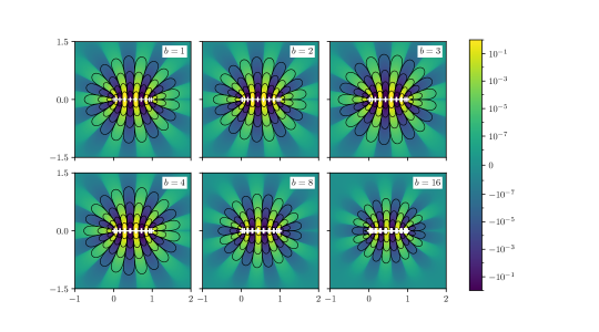
Figure 1: Imaginary part of the top-left entry of $f(z)\textup{{err}}_{k}(z)$ near the spectrum of $\mathbf{H}$ for block size $b=1,2,3,4,8,16$. Note that larger oscillations will result in more slack in the triangle inequality used between Equation 7 and Equation 8.

There are two main sources of slack in our bound. The first is from Equation 7 to Equation 8 due to losses associated with bounding the norm of an integral with the integral of a norm, and the second is from Equation 8 to the result of Theorem 1 due to potential slackness in a sub-multiplicative bound. With block size introduced to the Lanczos algorithm, an interesting question that arises is the impact of block size on the bound given by Theorem 1. In our first experiment, we illustrated relevant quantities for a range of block sizes to illustrate how the block size impacts our bound. For experiments in this section, we use the square root function $f(x)=\sqrt{x}$. We take $\mathbf{V}$ to be an $n\times b$ block-vector with independent standard Gaussian entries, and $w=0$. We set $\mathbf{H}$ to be a $1000\times 1000$ diagonal matrix with linearly spaced diagonal elements between $10^{-2}$ and 1. We will investigate the slackness in our bound across block sizes $b=1,2,3,4,8,16$. Reorthogonalization is used.

We first study the loss from the triangle inequality between Equation 7 and Equation 8. The error introduced by triangle inequality is larger when the function is more oscillatory over the contour. In fact, by the Cauchy–Schwarz inequality, Equation 7 and Equation 8 would be identical only if both real and imaginary parts of the integrand of Equation 7 were constant at every point on the contour.

In Figure 1, we plot the imaginary part of the top-left entry of $f(z)\textup{{err}}_{k}(z)$ on $0\leq\operatorname{Re}(z)\leq 1$ and $0\leq\operatorname{Im}(z)\leq 1$. From Figure 1, we observe that the sign of this entry of the integrand of Equation 7 oscillates as rays shoot out of eigenvalues of $\mathbf{H}$. Furthermore, the oscillation has a larger magnitude near the $\Lambda(\mathbf{H})$, and the magnitude decreases as we move away from $\Lambda(\mathbf{H})$. Most importantly, the qualitative behavior of the plot is similar across block sizes, so block size is not a factor that significantly impacts how we should choose the contour $\Gamma$ to reduce the error introduced by the triangle inequality. The real and imaginary parts of other entries of $f(z)\textup{{err}}_{k}(z)$ exhibit similar behavior.

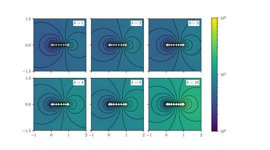
Figure 2: Ratio $T(z)$ defined in Equation 17 (with $w=\lambda_{\textup{min}}/100$) near the spectrum of $\mathbf{H}$ for block sizes $b=1,2,3,4,8,16$. Note that larger values of $T(z)$ result in more slack between Equation 8 and the result of Theorem 1.

To evaluate the difference between the bound defined in Equation 8 and (9), we define

$$T(z)={\|h_{w,z}(\mathbf{H})\|_{2}\|\mathbf{C}(w)^{-1}\mathbf{C}(z)\|_{2}\|\textup{{err}}_{k}(w)\|}{\|\textup{{err}}_{k}(z)\|}^{-1}.$$ (17)

The value of $T(z)$ at a point $z$ is the ratio between the integrands of Equation 8 and (9). If $T(z)=1$ for all points on the contour, then Equation 8 and Equation 9 would be identical. Since Equation 9 is identical to the result of Theorem 1, this ratio at a value $z$ offers us insights into the local difference between our bound and Equation 8.

We plot the ratio $T(z)$ under the same condition as Figure 1. Quantitatively, as block size $b$ increases, the ratio increases. This indicates that large block sizes render our error bound less precise under the same contour and choice of $w$, but the optimal contour $\Gamma$ is similar across various block sizes $b$. Furthermore, the slack ratio has a singularity and is large near the eigenvalue of $\mathbf{H}$, while a small ratio is observed near $w=0$. As we move away from eigenvalues of $\mathbf{H}$ or toward $w=0$, the ratio decreases.

3.2 Impact of contour

Figure 3: Pac-Man contour with parameters $R$, $\Theta$, $O$

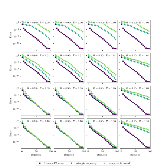
Figure 4: Performance of the Pac-Man contour across various parameters $R$ and $\Theta$ for $f(x)=\sqrt{x}$. The block-Lanczos-FA error is measured with $w=0$. The bound “triangle inequality” is Equation 8 and the bound “computable bound” is Theorem 1, both evaluated numerically. When $R$ and $\Theta$ are both reasonably large, the quality of the bounds is extremely good, but for some parameter choices, the bounds may have significant slack.

We now explore a family of contours and observe their impact on our computable bound in Theorem 1. Specifically, we will be focusing on the “Pac-Man contour”, which is the section of the circle $Re^{i\theta}+O$ with $-\Theta\leq\theta\leq\Theta$ and the lines between $O$ and $Re^{\pm i{\Theta}}$, for some $0<\Theta<\pi$. This contour is shown in Figure 3. To visualize the slackness of this family of contours, we plot the block-Lanczos-FA error Equation 5, triangle inequality error Equation 8, and our computable bound in Theorem 1 across block-Lanczos algorithm iterations between 0 and 100.

We can try to minimize the losses described in the previous section by optimizing the parameters $R$ and $\Theta$ for the Pac-Man contour. From Figure 1, since the magnitude of the oscillation decreases as the point of evaluation moves further from the spectrum of $\mathbf{H}$, it seems reasonable that a larger radius $R$ leads to a smaller triangle inequality error. Similar behavior is observed from Figure 2. Owing to the symmetry across the real axis, it seems reasonable to choose a real origin. Since the square root function has a branch cut at the negative real axis and the origin is a point for the integral term to be evaluated, the origin cannot be on the negative real axis. But making it too close to the spectrum will also cause our bounds to deteriorate.

According to the constraints above, we choose our origin to be $O={\lambda_{\textup{min}}}/{100}$, and allow $R$ and $\Theta$ to vary with $R>\lambda_{\textup{max}}-O$, and $\pi<\theta<0$. We then evaluate the performance of Theorem 1 with the same matrix $\mathbf{H}$, block-vector $\mathbf{V}$, and parameter $w=0$ as in Section 3.1, and show the results in Figure 4. In the previous experiments, we have established empirically that block size does not have a large qualitative impact on the behavior of Theorem 1 for this example. Thus, we choose a fixed block size $b=4$ to focus on the impacts of the contour.

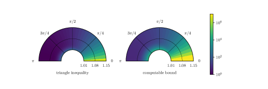
Figure 5: Bound divided by block-Lanczos-FA for the Pac-Man contour across various parameters $R$ and $\Theta$ for $f(x)=\sqrt{x}$ at $k=30$. The block-Lanczos-FA error is measured with $w=0$. The bound “triangle inequality” is Equation 8 and the bound “computable bound” is Theorem 1 evaluated numerically.

Overall, as $k$ increases, the computable bound remains near or converges to the triangle inequality error, while the triangle inequality error remains near or diverges from the block-Lanczos-FA error. Across each column of Figure 4, we observe that with a larger radius, both the triangle inequality error and computable bound converge to block-Lanczos-FA error, offering a tighter bound, which matches our observations from Figure 1 and Figure 2. Across each row of Figure 4, with larger $\Theta$ value, both triangle inequality error and computable bound move further from block-Lanczos-FA error, less to less accurate bound. This is because by the construction of the Pac-Man contour, with smaller $\Theta$ values (especially with $0<\Theta<\frac{\pi}{2}$), the line between $O$ and $Re^{i{\Theta}}$ and between $O$ and $Re^{-i{\Theta}}$ move closer to the spectrum of $\mathbf{H}$. This increases the triangle inequality error and computable bound as observed in Figure 1 and Figure 2, which gives us the behavior observed in the last column of Figure 4.

To better visualize our claim, we focus on the performance of Theorem 1 with the block-Lanczos algorithm at $k=30$ iterations. Under the same construction as Figure 4, we plot the ratio between triangle inequality error and block-Lanczos-FA error, and between computable bound and block-Lanczos-FA error across different values of $R$ and $\Theta$ as Figure 5. We observe that a larger radius leads to a ratio closer to 1 between triangle inequality error and block-Lanczos-FA error and between computable bound and block-Lanczos-FA error, which matches our observation in Figure 4. Furthermore, in general, smaller values of $\Theta$ leads to worse performance. However, when $\Theta>\frac{\pi}{2}$, the performance is rather similar across different values of $\Theta$. This matches our expectations, and suggests that our bounds do not require significant tuning.

3.3 Sign Function

We now study the behavior of our bound on the sign function, another function widely used in a number of application areas. In particular, we consider the approximation of $\operatorname{sign}(\mathbf{H})\mathbf{V}$, where $\mathbf{H}$ is the Wilson fermion matrix from Quantum Chromodynamics (QCD). This quantity is required as part of a larger algorithm in QCD [vdEFL⁺02, FS08b].

For this example, we use $\mathbf{H}=\mathbf{P}(\mathbf{I}-\frac{4}{3}k\mathbf{D})$, where $\mathbf{D}$ is from the QCD collection of the matrix market with file name conf5.0-00l4x4-1000.mtx with $k=0.20611$. $\mathbf{P}$ is the permutation matrix given by

$$\mathbf{P}=\mathbf{I}_{3}\otimes\begin{pmatrix}0&0&1&0\\ 0&0&0&1\\ 1&0&0&0\\ 0&1&0&0\end{pmatrix}\otimes\mathbf{I}_{256}.$$

Let $f(x)$ be the step function; $f(x)=1$ for $x\geq 0$ and $f(x)=0$ for $x<0$. Then $\operatorname{sign}(x)=2f(x)-1$. Since block-Lanczos-FA is linear in the input function, and since the algorithm applies low-degree polynomials (such as $x\mapsto-1$) exactly,

$$\operatorname{sign}(\mathbf{H})\mathbf{V}-\textup{{lan}}_{k}(\operatorname{sign})=2f(\mathbf{H})\mathbf{V}-\mathbf{V}-\big{(}2\textup{{lan}}_{k}(f)-\mathbf{V}\big{)}=2\big{(}f\mathbf{A})\mathbf{V}-\textup{{lan}}_{k}(f)\big{)}.$$

Thus, it suffices to study the behavior of block-Lanczos-FA on the step function.

In order to apply Theorem 1, we require $f$ to be analytic on the interiors of each of the closed curves in the contour $\Gamma$. Extend $f$ to the complex plane by $f(z)=1$ for all $z$ such that $\operatorname{Re}(z)\geq 0$, $f(z)=0$ for all $z$ such that $\operatorname{Re}(z)<0$. Assuming $\Lambda(\mathbf{H})$ and $\Lambda(\mathbf{T})$ are bounded away from zero, we can take $\Gamma$ as the union of two simple closed curves; one encircling $[\lambda_{\textup{min}},-\epsilon]$ and one encircling $[\epsilon,\lambda_{\textup{max}}]$, where $\epsilon>0$ is some sufficiently small value. When we apply Theorem 1, the first contour can be ignored, as $f(z)=0$ for all $z$ on the contour.

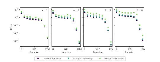
Figure 6: Convergence of the block-Lanczos algorithm for block sizes $b=1,2,4,8$ for the step function $f(x)=1$ if $x>0$ and $f(x)=0$ if $x\leq 0$. The contour used is the Pan-Man contour centered at 0 with $R=2\lambda_{\textup{max}}$ and $\Theta=\frac{1}{2}\pi$. The block-Lanczos-FA error is measured using $\|\cdot\|_{\mathbf{I}}=\|\cdot\|_{\mathsf{F}}$. The bound “triangle inequality” is Equation 8 and the bound “computable bound” is Theorem 1, both evaluated numerically. While there is some deterioration of the bounds as the block size increases, the computable bound appears suitable for use as a stopping criterion.

We investigate the impact of block size on this example problem using a Pac-Man contour centered at $0$ with $\Theta=0.5\pi$ and a radius $R=2\lambda_{\textup{max}}$ large enough to cover all eigenvalues of $\mathbf{H}$. Note that with $\Theta=0.5\pi$, the Pac-Man contour shapes like the letter ”D” and never intersects with the imaginary axis. In Figure 6, we plot the rate of convergence of the block Lanczos algorithm and our bound Theorem 1, where $\mathbf{V}$ is a block-vector of random Gaussian entries. We note that the number of iterations required to converge is almost inversely proportional to the block size. This shows that having larger block sizes significantly decreases the number of matrix loads without increasing the total number of matrix-vector products significantly. Thus, bounds such as Equation 3, which would not change significantly in the different cases, cannot be descriptive of the convergence. Our bounds are qualitatively similar in all cases, degrading slightly with the block size. In this particular example, such degradation is not of major concern, as convergence is very sudden after a certain critical number of iterations have been performed.

3.4 Quadratic forms

In this section we use the same matrix as in Section 3.1 with $f(x)=1/\sqrt{x}$ and compute bounds for the quadratic form error $\|\mathbf{V}^{*}f(\mathbf{H})\mathbf{V}-\mathbf{V}^{*}\textup{{lan}}_{k}(f)\|_{2}$. We use a Pac-Man contour centered at $0$ with $\Theta=0.5\pi$ and a radius $R=2\lambda_{\textup{max}}$ and test our bounds for several block sizes. The results of our experiments are shown in Figure 7. As in other experiments, we observe qualitatively similar results in all cases, with some deterioration as the block size increases.

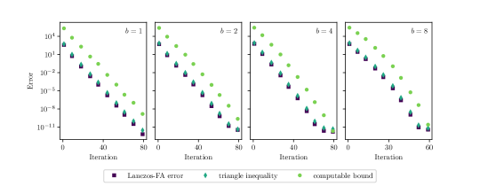
Figure 7: Convergence of the block-Lanczos algorithm for “quadratic forms” for block sizes $b=1,2,4,8$ for $f(x)=1/\sqrt{x}$. The contour used is the Pan-Man contour centered at 0 with $R=2\lambda_{\textup{max}}$ and $\Theta=\frac{\pi}{2}$. The block-Lanczos-FA error is measured using $\|\cdot\|_{2}$. The bound “triangle inequality” is Equation 10 and the bound “computable bound” is Equation 11, both evaluated numerically.

3.5 Finite precision arithmetic

In this experiment, we consider the impact of reorthogonalization in the block-Lanczos algorithm on the quality of our bounds. We again take $\mathbf{V}$ to have $b=4$ columns with independent Gaussian entries and set the eigenvalues of $\mathbf{H}$ to those of the model problem [Str91, SG92]. Explicitly, the eigenvalues are

$$\lambda_{1}=1/\kappa,\qquad\lambda_{n}=1,\qquad\lambda_{i}=\lambda_{1}+\left(\frac{i-1}{n-1}\right)\cdot(\lambda_{n}-\lambda_{1})\cdot\rho^{n-i},\qquad i=2,\ldots,n-1.$$

In our experiment, we use parameters $n=500$, $\kappa=10^{3}$, and $\rho=0.9$ and set $f(x)=1/\sqrt{x}$. We run the block-Lanczos-FA algorithm to convergence with and without reorthogonalization and report the results of our bounds with a Pac-Man contour with $\Theta=\pi/100$ and $R=2$ in Figure 8.

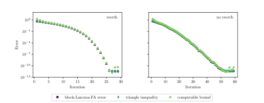
Figure 8: Comparison between the rate of convergence of the block-Lanczos algorithm with and without reorganization for $f(x)=\sqrt{x}$ with block size $b=4$. The contour used is the Pac-Man contour centered at ${\lambda_{\textup{min}}}/{100}$ with $R=2$ and $\Theta=\frac{1}{100}\pi$. The block-Lanczos-FA error is measured with $w={\lambda_{\textup{min}}}/{100}$. The bound “triangle inequality” is Equation 8 and the bound “computable bound” is Theorem 1 evaluated numerically.

Note that the convergence of the block-Lanczos-FA algorithm is delayed when reorthogonalization is not used. However, the algorithm still converges. In both cases, our bound performs well, tracking the actual convergence of the algorithm. This aligns with our expectations from the rounding error analysis performed in Section 2.2 and provides further evidence supporting the potential value of our bound as a practical stopping criterion.

4 Conclusion and outlook

In this paper, we gave an error bound for block-Lanczos-FA used to approximate $f(\mathbf{H})\mathbf{V}$ with piece-wise analytic function $f$. We analyzed the behavior of our error bound and established that block size does not qualitatively alter the behavior of our error bound; the bounds remain reasonably sharp in all cases. This allows us to evaluate the behavior of our error bound with a fixed block size, and generalize our findings to other block sizes. To better understand the impact of contours on our error bound, we investigated the family of the Pac-Man contours and studied its parameters’ impact on the slackness of our bound based on our experiments. This offered us insights into the qualitative behavior of the contour near the spectrum of $\mathbf{H}$ and allowed us to choose parameters of the Pac-Man contour that tighten our bound.

In the future, we have two main goals. We will analyze the performance of different combinations of values of $w$ and contour, and look into various other functions, including the sign function, to study the performance of the error bound on a wider range of examples.

5 Statements and Declarations

The authors have no competing interests to declare that are relevant to the content of this article.

All data generated or analyzed during this study are included in this published article.

Appendix A Estimates for the block-CG error norm

In this section, we discuss how to obtain an error estimate for the $(\mathbf{H}-w\mathbf{I})$-norm of the error of the block-Lanczos algorithm used to approximate $(\mathbf{H}-w\mathbf{I})^{-1}\mathbf{V}$; i.e. with $f(x)=(x-w)^{-1}$. For simplicity, without loss of generality, we will assume $w=0$. Closely related approaches are widely studied for the block size one case [ST02, MT18, EOS19, MPT21, MT22]. Bounds for the block algorithm have also been studied [SST21].

By a simple triangle inequality, we obtain a bound

$$\|\textup{{err}}_{k}(w)\|_{\mathbf{H}} =\|\mathbf{H}^{-1}\mathbf{V}-\textup{{lan}}_{k}(f)\|_{\mathbf{H}}$$

$$\leq\|\mathbf{H}^{-1}\mathbf{V}-\textup{{lan}}_{k+d}(f)\|_{\mathbf{H}}+\|\textup{{lan}}_{k+d}(f)-\textup{{lan}}_{k}(f)\|_{\mathbf{H}}.$$

If we assume that $d$ is chosen sufficiently large so that

$$\|\mathbf{H}^{-1}\mathbf{V}-\textup{{lan}}_{k+d}(f)\|_{\mathbf{H}}\ll\|\textup{{lan}}_{k+d}(f)-\textup{{lan}}_{k}(f)\|_{\mathbf{H}},$$

then we obtain an approximate error bound (error estimate)

$$\|\textup{{err}}_{k}(w)\|_{\mathbf{H}}\lesssim\|\textup{{lan}}_{k+d}(f)-\textup{{lan}}_{k}(f)\|_{\mathbf{H}}.$$ (18)

It is natural to ask why we don’t simply apply this approach to the block-Lanczos-FA algorithm for any function $f$. Such an approach was suggested for the Lanczos-FA algorithm in [ER21], and in many cases can work well. However, if the convergence of the block-Lanczos-FA algorithm is not monotonic, then the critical assumption that $\textup{{lan}}_{k+d}(f)$ is a much better approximation to $f(\mathbf{H})\mathbf{V}$ than $\textup{{lan}}_{k}(f)$ may not hold. Perhaps more importantly, the decomposition in Theorem 1 also allows intuition about how the distribution of eigenvalues of $\mathbf{H}$ impact the convergence of block-CG to be extended to the block-Lanczos-FA algorithm.

In Figure 9 we show a numerical experiment illustrating the quality of Equation 18 for several values of $d$. As expected, increasing $d$ improves the quality of the estimate. However, even for small $d$, Figure 9 appears suitable for use as a practical stopping criterion on this problem. Of course, on problems where the convergence of block-CG stagnates, such an error estimate will require $d$ fairly large. Further study of this topic is outside the scope of the present paper.

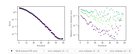
Figure 9: Illustration of the quality of Figure 9 for varying $d$. The block-Lanczos-FA error is measured using $\|\cdot\|_{\mathbf{H}-w\mathbf{I}}$ with $w=0$.

Appendix B Proof of Equation 3

Owing to linearity, in order to show $p(\mathbf{H})\mathbf{V}=\textup{{lan}}_{k}(p)$ for any polynomial $p$ with $\deg(p)<k$, it suffices to consider the case $p(x)=x^{j}$, for $j=0,\ldots,k-1$. Left multiplying Equation 2 by $\mathbf{H}^{j-1}$ and then repeatedly applying Equation 2 we find

$$\mathbf{H}^{j}\mathbf{Q} =\mathbf{H}^{j-1}\mathbf{Q}\mathbf{T}+\mathbf{H}^{j-1}\mathbf{Q}_{k+1}\mathbf{B}_{k}\mathbf{E}_{k}^{*}$$

$$=\mathbf{H}^{j-2}(\mathbf{Q}\mathbf{T}+\mathbf{Q}_{k+1}\mathbf{B}_{k}\mathbf{E}_{k}^{*})\mathbf{T}+\mathbf{H}^{j-1}\mathbf{Q}_{k+1}\mathbf{B}_{k}\mathbf{E}_{k}^{*}$$

$$\mathmakebox[width("{}={}")][c]{\vdots}$$

$$=\mathbf{Q}\mathbf{T}^{j}+\sum_{i=1}^{j}\mathbf{H}^{j-i}\mathbf{Q}_{k+1}\mathbf{B}_{k}\mathbf{E}_{k}^{*}\mathbf{T}^{i-1}.$$

Thus, using that $\mathbf{V}=\mathbf{Q}\mathbf{E}_{1}\mathbf{B}_{0}$,

$$\mathbf{H}^{j}\mathbf{V}=\mathbf{H}^{j}\mathbf{Q}\mathbf{E}_{1}\mathbf{B}_{0}=\mathbf{Q}\mathbf{T}^{j}\mathbf{E}_{1}\mathbf{B}_{0}+\sum_{i=1}^{j}\mathbf{H}^{j-i}\mathbf{Q}_{k+1}\mathbf{B}_{k}\mathbf{E}_{k}^{*}\mathbf{T}^{i-1}\mathbf{E}_{1}\mathbf{B}_{0}.$$

Since $\mathbf{T}$ is banded with half bandwidths $b$, $\mathbf{T}^{i-1}$ is banded with half bandwidth $(i-1)b$. Thus, the bottom left $b\times b$ block of $\mathbf{T}^{i-1}$ is all zero provided $i-1\leq k-2$; i.e. $\mathbf{E}_{k}^{*}\mathbf{T}^{i-1}\mathbf{E}_{1}\mathbf{B}_{0}=\mathbf{0}$ provided $i<k$. We therefore find that for all $j<k$,

$$\mathbf{H}^{j}\mathbf{V}=\mathbf{Q}\mathbf{T}^{j}\mathbf{E}_{1}\mathbf{B}_{0},$$

from which we infer $p(\mathbf{H})\mathbf{V}=\textup{{lan}}_{k}(p)$ for any $p$ with $\deg(p)<k$.

Therefore, using the triangle inequality, for any polynomial $p$ with $\deg(p)<k$,

$$\|f(\mathbf{H})\mathbf{V}-\textup{{lan}}_{k}(f)\|_{2} =\|f(\mathbf{H})\mathbf{V}-\mathbf{Q}f(\mathbf{T})\mathbf{E}_{1}\mathbf{B}_{0}\|_{2}$$

$$\leq\|f(\mathbf{H})\mathbf{V}-p(\mathbf{H})\mathbf{V}\|+\|\mathbf{Q}p(\mathbf{T})\mathbf{E}_{1}\mathbf{B}_{0}-\mathbf{Q}f(\mathbf{T})\mathbf{E}_{1}\mathbf{B}_{0}\|_{2}$$

$$\leq\|f(\mathbf{H})-p(\mathbf{H})\|_{2}\|\mathbf{V}\|_{2}+\|\mathbf{Q}\|_{2}\|p(\mathbf{T})-f(\mathbf{T})\|\|\mathbf{E}_{1}\mathbf{B}_{0}\|_{2}.$$

$$\leq\|\mathbf{V}\|_{2}\left(\|f(\mathbf{H})-p(\mathbf{H})\|_{2}+\|p(\mathbf{T})-f(\mathbf{T})\|_{2}\right).$$

In the final inequality we have use that $\|\mathbf{Q}\|\leq 1$ since $\mathbf{Q}$ has orthonormal columns and that $\|\mathbf{E}_{1}\mathbf{B}_{0}\|=\|\mathbf{Q}^{*}\mathbf{V}\|\leq\|\mathbf{V}\|$. Next, note that

$$\|f(\mathbf{H})-p(\mathbf{H})\|_{2}=\max_{x\in\Lambda(\mathbf{H})}|f(x)-p(x)|,\qquad\|p(\mathbf{T})-f(\mathbf{T})\|_{2}=\max_{x\in\Lambda(\mathbf{T})}|f(x)-p(x)|$$

so, since each of $\Lambda(\mathbf{H})$ and $\Lambda(\mathbf{T})$ are contained in $[\lambda_{\textup{min}}(\mathbf{H}),\lambda_{\textup{max}}(\mathbf{H})]$, we find

$$\|f(\mathbf{H})\mathbf{V}-\textup{{lan}}_{k}(f)\|_{2} \leq 2\|\mathbf{V}\|\max_{x\in[\lambda_{\textup{min}}(\mathbf{H}),\lambda_{\textup{max}}(\mathbf{H})]}|f(x)-p(x)|.$$

Since $p$ was arbitrary, we can optimize over all polynomials $p$ with $\deg(p)<k$.

References

• [ACSS12] Tadashi Ando, Edmond Chow, Yousef Saad, and Jeffrey Skolnick. Krylov subspace methods for computing hydrodynamic interactions in brownian dynamics simulations. The Journal of Chemical Physics, 137(6):064106, August 2012.
• [BBJ15] H. Barkouki, A. H. Bentbib, and K. Jbilou. An adaptive rational block Lanczos-type algorithm for model reduction of large scale dynamical systems. Journal of Scientific Computing, 67(1):221–236, July 2015.
• [BFG96] Zhaojun Bai, Gark Fahey, and Gene Golub. Some large-scale matrix computation problems. Journal of Computational and Applied Mathematics, 74(1-2):71–89, November 1996.
• [Bir18] Sebastian Birk. Deflated shifted block Krylov subspace methods for Hermitian positive definite matrices. 2018.
• [CC22] Tyler Chen and Yu-Chen Cheng. Numerical computation of the equilibrium-reduced density matrix for strongly coupled open quantum systems. The Journal of Chemical Physics, 157(6):064106, August 2022.
• [CGMM22] Tyler Chen, Anne Greenbaum, Cameron Musco, and Christopher Musco. Error bounds for Lanczos-based matrix function approximation. SIAM Journal on Matrix Analysis and Applications, 43(2):787–811, May 2022.
• [CH22] Tyler Chen and Eric Hallman. Krylov-aware stochastic trace estimation, 2022.
• [CLS22] Erin Carson, Jörg Liesen, and Zdeněk Strakoš. 70 years of Krylov subspace methods: The journey continues, 2022.
• [DK92] Vladimir Druskin and Leonid Knizhnerman. Error bounds in the simple Lanczos procedure for computing functions of symmetric matrices and eigenvalues. Comput. Math. Math. Phys., 31(7):20–30, July 1992.
• [DV95] Luca Dieci and Erik S. Van Vleck. Computation of a few lyapunov exponents for continuous and discrete dynamical systems. Applied Numerical Mathematics, 17(3):275–291, July 1995.
• [EOS19] Ron Estrin, Dominique Orban, and Michael Saunders. Euclidean-norm error bounds for SYMMLQ and CG. SIAM Journal on Matrix Analysis and Applications, 40(1):235–253, January 2019.
• [ER21] Nasim Eshghi and Lothar Reichel. Estimating the error in matrix function approximations. Advances in Computational Mathematics, 47(4), August 2021.
• [FGS14] Andreas Frommer, Stefan Güttel, and Marcel Schweitzer. Convergence of restarted Krylov subspace methods for Stieltjes functions of matrices. SIAM Journal on Matrix Analysis and Applications, 35(4):1602–1624, January 2014.
• [FKLR13] Andreas Frommer, Karsten Kahl, Th Lippert, and Hannah Rittich. 2-norm error bounds and estimates for Lanczos approximations to linear systems and rational matrix functions. SIAM Journal on Matrix Analysis and Applications, 34(3):1046–1065, 2013.
• [FLS17] Andreas Frommer, Kathryn Lund, and Daniel B. Szyld. Block Krylov subspace methods for functions of matrices. Electron. Trans. Numer. Anal., 47:100–126, 2017.
• [FMR16] Paraskevi Fika, Marilena Mitrouli, and Paraskevi Roupa. Estimating the diagonal of matrix functions. Mathematical Methods in the Applied Sciences, 41(3):1083–1088, October 2016.
• [FS08a] Andreas Frommer and Valeria Simoncini. Stopping criteria for rational matrix functions of Hermitian and symmetric matrices. SIAM Journal on Scientific Computing, 30(3):1387–1412, January 2008.
• [FS08b] Andreas Frommer and Valeria Simoncini. Stopping criteria for rational matrix functions of Hermitian and symmetric matrices. SIAM Journal on Scientific Computing, 30(3):1387–1412, Jan 2008.
• [FS09] Andreas Frommer and Valeria Simoncini. Error bounds for Lanczos approximations of rational functions of matrices. In Numerical Validation in Current Hardware Architectures, pages 203–216, Berlin, Heidelberg, 2009. Springer Berlin Heidelberg.
• [FS15] Andreas Frommer and Marcel Schweitzer. Error bounds and estimates for Krylov subspace approximations of Stieltjes matrix functions. BIT Numerical Mathematics, 56(3):865–892, December 2015.
• [GM09] Gene H Golub and Gérard Meurant. Matrices, moments and quadrature with applications, volume 30. Princeton University Press, 2009.
• [Gre97] Anne Greenbaum. Iterative Methods for Solving Linear Systems. Society for Industrial and Applied Mathematics, Philadelphia, PA, USA, 1997.
• [GU77] G.H. Golub and R. Underwood. The block Lanczos method for computing eigenvalues. In Mathematical Software, pages 361–377. Elsevier, 1977.
• [ITS09] Marija D. Ilic, Ian W. Turner, and Daniel P. Simpson. A restarted Lanczos approximation to functions of a symmetric matrix. IMA Journal of Numerical Analysis, 30(4):1044–1061, June 2009.
• [LM16] Steven Cheng-Xian Li and Benjamin M Marlin. A scalable end-to-end Gaussian process adapter for irregularly sampled time series classification. In D. Lee, M. Sugiyama, U. Luxburg, I. Guyon, and R. Garnett, editors, Advances in Neural Information Processing Systems, volume 29. Curran Associates, Inc., 2016.
• [MMMW21] Raphael A Meyer, Cameron Musco, Christopher Musco, and David P Woodruff. Hutch++: Optimal stochastic trace estimation. In Symposium on Simplicity in Algorithms (SOSA), pages 142–155. SIAM, 2021.
• [MMS18] Cameron Musco, Christopher Musco, and Aaron Sidford. Stability of the Lanczos method for matrix function approximation. In Proceedings of the Twenty-Ninth Annual ACM-SIAM Symposium on Discrete Algorithms, SODA ’18, page 1605–1624, USA, 2018. Society for Industrial and Applied Mathematics.
• [MPT21] Gérard Meurant, Jan Papež, and Petr Tichý. Accurate error estimation in CG. Numerical Algorithms, April 2021.
• [MT18] Gérard Meurant and Petr Tichý. Approximating the extreme Ritz values and upper bounds for the ${A}$-norm of the error in CG. Numerical Algorithms, 82(3):937–968, November 2018.
• [MT22] Gérard Meurant and Petr Tichý. The behaviour of the Gauss–Radau upper bound of the error norm in cg, 2022.
• [O'L80] Dianne P. O'Leary. The block conjugate gradient algorithm and related methods. Linear Algebra and its Applications, 29:293–322, February 1980.
• [Pai71] Christopher Conway Paige. The computation of eigenvalues and eigenvectors of very large sparse matrices. PhD thesis, University of London, 1971.
• [Pai76] Christopher Conway Paige. Error analysis of the Lanczos algorithm for tridiagonalizing a symmetric matrix. IMA Journal of Applied Mathematics, 18(3):341–349, 12 1976.
• [Pai80] Christopher Conway Paige. Accuracy and effectiveness of the Lanczos algorithm for the symmetric eigenproblem. Linear Algebra and its Applications, 34:235 – 258, 1980.
• [Saa92] Yousef Saad. Analysis of some Krylov subspace approximations to the matrix exponential operator. SIAM Journal on Numerical Analysis, 29(1):209–228, 1992.
• [SG92] Zdenek Strakos and Anne Greenbaum. Open questions in the convergence analysis of the Lanczos process for the real symmetric eigenvalue problem. University of Minnesota, 1992.
• [SRS20] Jürgen Schnack, Johannes Richter, and Robin Steinigeweg. Accuracy of the finite-temperature Lanczos method compared to simple typicality-based estimates. Physical Review Research, 2(1), February 2020.
• [SST21] Christian E. Schaerer, Daniel B. Szyld, and Pedro J. Torres. A posteriori superlinear convergence bounds for block conjugate gradient, 2021.
• [ST02] Zdeněk Strakoš and Petr Tichỳ. On error estimation in the conjugate gradient method and why it works in finite precision computations. ETNA. Electronic Transactions on Numerical Analysis [electronic only], 13:56–80, 2002.
• [Str91] Zdenek Strakos. On the real convergence rate of the conjugate gradient method. Linear Algebra and its Applications, 154-156:535 – 549, 1991.
• [SY20] Kazuhiro Seki and Seiji Yunoki. Thermodynamic properties of an $s=\frac{1}{2}$ ring-exchange model on the triangular lattice. Physical Review B, 101(23), June 2020.
• [Und75] Richard Ray Underwood. An Iterative Block Lanczos Method for the Solution of Large Sparse Symmetric Eigenproblems. PhD thesis, Stanford, CA, USA, 1975. AAI7525622.
• [vdEFL+02] J. van den Eshof, A. Frommer, Th. Lippert, K. Schilling, and H.A. van der Vorst. Numerical methods for the QCDd overlap operator. I. Sign-function and error bounds. Computer Physics Communications, 146(2):203 – 224, 2002.