Separating the blue cloud and the red sequence using Otsu’s method for image segmentation

Abstract

The observed colour bimodality allows a classification of the galaxies into two distinct classes: the ‘blue cloud’ and the ‘red sequence’. Such classification is often carried out using empirical cuts in colour and other galaxy properties that lack solid mathematical justifications. We propose a method for separating the galaxies in the ‘blue cloud’ and the ‘red sequence’ using Otsu’s thresholding technique for image segmentation. We show that this technique is insensitive to the choice of binning. It provides a robust and parameter-free method for the classification of the red and blue galaxies based on the minimization of the intra-class variance and maximization of the inter-class variance. We also apply an iterative triclass thresholding technique based on Otsu’s method to improve the classification. The galaxy colour is known to depend on the stellar mass and the luminosity of galaxies. We obtain the dividing lines between the two populations in the colour-stellar mass plane and the colour-absolute magnitude plane by employing these methods in a number of independent stellar mass bins and absolute magnitude bins.

organization= Department of Physics, Visva-Bharati University,addressline=, city=Santiniketan, postcode=731235, state=West Bengal, country=India

1 Introduction

The galaxies are the fundamental unit of the large-scale structures. They come in various shapes, sizes, luminosity, mass, colour, star formation rate and metallicity. Classifying the galaxies based on their physical properties helps us to understand their formation and evolution.

The colour of a galaxy is defined as the ratio of fluxes in two different filters. It is considered one of the fundamental properties of a galaxy that characterizes its stellar population. It is now well known that the observed distribution of galaxy colour is strongly bimodal (Strateva, et al., 2001; Blanton, et al., 2003; Bell, et al., 2003; Balogh, et al., 2004; Baldry, et al., 2004). The observed colour distribution reveals two distinct peaks corresponding to a ‘blue cloud’ and a ‘red sequence’. The ‘blue cloud’ predominantly hosts the active star-forming galaxies with younger stellar populations, lower stellar mass and disk-like morphology (Strateva, et al., 2001; Blanton, et al., 2003; Kauffmann et al., 2003; Baldry, et al., 2004). On the other hand, the galaxies in the ‘red sequence’ have higher stellar mass with an older stellar population and bulge-dominated morphology.

The bimodal character of the galaxy colour distribution has important implications for galaxy formation and evolution. The colour bimodality is known to exist out to $z=1-2$ (Bell, et al., 2004; Brammer et al., 2009). Observations indicate that the number of massive red galaxies has increased steadily since $z\sim 1$ (Bell, et al., 2004; Faber et al., 2007). It indicates that the blue galaxies transform into red ones via the quenching of star formation. Such quenching may happen through different physical processes and mechanisms. A sharp decline in star formation rate between $z=1$ to present (Madau et al., 1996) also hints towards a significant evolution of the galaxy properties. Such evolution may have played a decisive role in shaping the observed colour bimodality in the present Universe. The colour bimodality also depends on luminosity, stellar mass and environment (Balogh, et al., 2004; Baldry, et al., 2006; Pandey & Sarkar, 2020). Any successful model of galaxy formation must be able to reproduce the observed colour bimodality. The semi-analytic models of galaxy formation has been widely used in a number of works to explain the observed colour bimodality (Menci, et al., 2005; Driver, et al., 2006; Cattaneo, et al., 2006, 2007; Cameron, et al., 2009; Trayford et al., 2016; Nelson, et al., 2018; Correa, Schaye & Trayford, 2019).

The red and blue galaxies are known to have different two-point correlation function (Zehavi, et al., 2011), three-point correlation function (Kayo, et al., 2004), genus (Hoyle et al., 2002), filamentarity (Pandey & Bharadwaj, 2006), local dimension (Pandey & Sarkar, 2020) and mass function (Drory, et al., 2009; Taylor et al., 2015). These measurements provide important inputs to the theories of galaxy formation and evolution. One requires an operational definition of the two classes of galaxies in all such studies. Separating the blue and red galaxies is not a trivial task, as no galaxies can be regarded as either truly ‘blue’ or ‘red’ based on their colours. The primary motivation for such a classification lies in the observed bimodality of the colour distribution. The galaxies in the ‘blue cloud’ and the ‘red sequence’ are usually separated using specific cuts based on empirical arguments (Strateva, et al., 2001; Baldry, et al., 2004; Williams et al., 2009; Bamford et al., 2009; Arnouts et al., 2013; Fritz et al., 2014). For instance, Strateva, et al. (2001) proposed that the red and blue galaxies can be optimally separated using a colour cut of $(u-r)=2.22$. Pandey (2020) propose a fuzzy set theory-based method for classifying the red, blue and transition valley galaxies. Nevertheless, this method also has some arbitrariness in selecting the membership function and the associated parameters. A number of works have been carried out to distinguish the red and blue galaxy populations in the GAMA survey. Taylor et al. (2015) use the phenomenology of the colour–mass diagrams to provide objective operational definitions for the red and blue galaxies in the GAMA survey. Bremer et al. (2018) divide the galaxies into three broad colour bins corresponding to red, green and blue galaxies based on the surface density of points in the colour-mass plane. Turner et al. (2019) use k-means unsupervised clustering and Holwerda et al. (2022) use Self-Organizing Maps, an unsupervised machine learning technique to segregate the galaxies according to their properties. Ideally, it would be most desirable to have a method that can divide the two populations using some mathematically justified definition. One such method for statistical decision-making is Otsu’s thresholding technique (Otsu, 1979), originally proposed by Nobuyuki Otsu for image segmentation. It is a parameter-free method for separating the foreground pixels from the background. Over the years, it has found many important applications in remote sensing, robotic mapping and navigation and identifying tumors. The Otsu’s method has been also applied for object detection in astronomical images (Zheng et al., 2015; Gong et al., 2015).

In this work, we propose an automated method for separating the galaxies in the ‘blue cloud’ and the ‘red sequence’ for any given data set using Otsu’s algorithm (Otsu, 1979) for image segmentation. We also implement an improved iterative triclass thresholding technique (Cai et al., 2014) based on Otsu’s method to classify the red and blue galaxies. It provides a nearly parameter-free method for classifying the red and blue galaxies.

2 SDSS data

We apply the proposed method to the data from the Sloan Digital Sky Survey (SDSS) (York et al., 2000) which is the largest galaxy survey to date. It has collected the photometric and spectroscopic information of more than one million galaxies and quasars in five wave bands across one-quarter of the entire sky. We use the data from the SDSS DR16 (Ahumada et al., 2020) for the current work. We download the data from the SDSS SkyServer using SQL. We identify a contiguous region between the right ascension $135^{\circ}\leq\alpha\leq 225^{\circ}$ and the declination $0^{\circ}\leq\delta\leq 60^{\circ}$ and extract the spectroscopic information of all the galaxies with r-band Petrosian magnitude $13.5\leq r_{p}<17.77$ within redshift $z<0.3$. These cuts provide us with a total $376495$ galaxies. We then prepare a volume limited sample by applying a cut to the K-corrected and extinction corrected $r$-band absolute magnitude. We apply an absolute magnitude cut of $-21\geq M_{r}\geq-23$ that corresponds redshift limit $0.041\leq z\leq 0.120$. We finally have a total $103984$ galaxies in our volume limited sample. We download the stellar mass of these galaxies from a catalogue based on the Flexible Stellar Population Synthesis model (Conroy, Gunn & White, 2009). A $\Lambda$CDM cosmological model with $\Omega_{m0}=0.315$, $\Omega_{\Lambda 0}=0.685$ and $h=0.674$ (Planck Collaboration, et al., 2018) is used for our analysis. We used the same data set earlier to classify the red, green and blue galaxies using a fuzzy set theory based method (Pandey, 2020).

3 Method of Analysis

Figure 1: This shows the $(u-r)$ colour distribution of the SDSS galaxies in our volume limited sample.

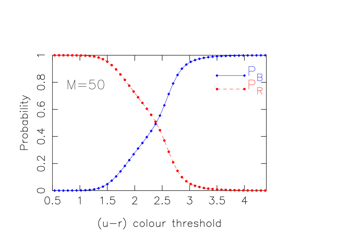
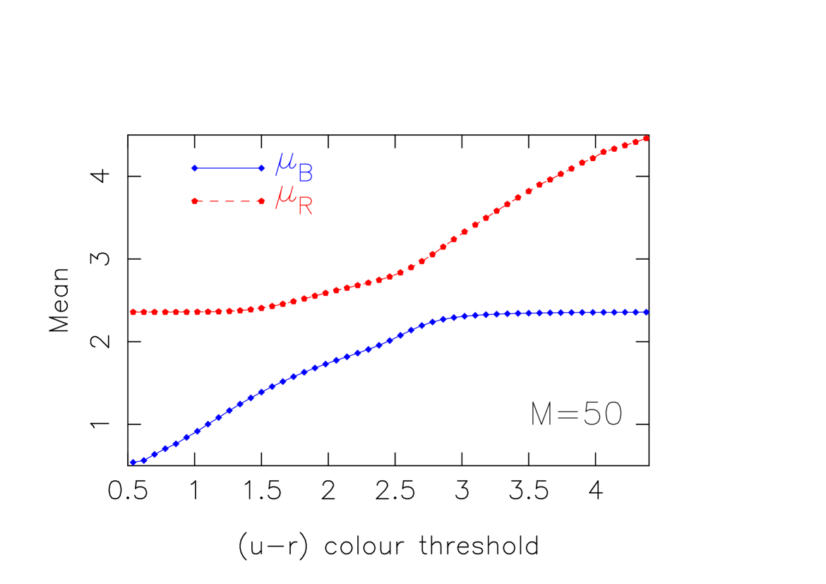
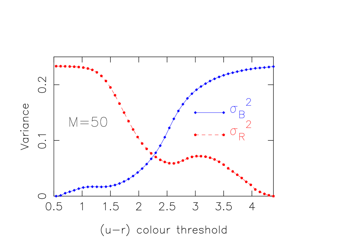
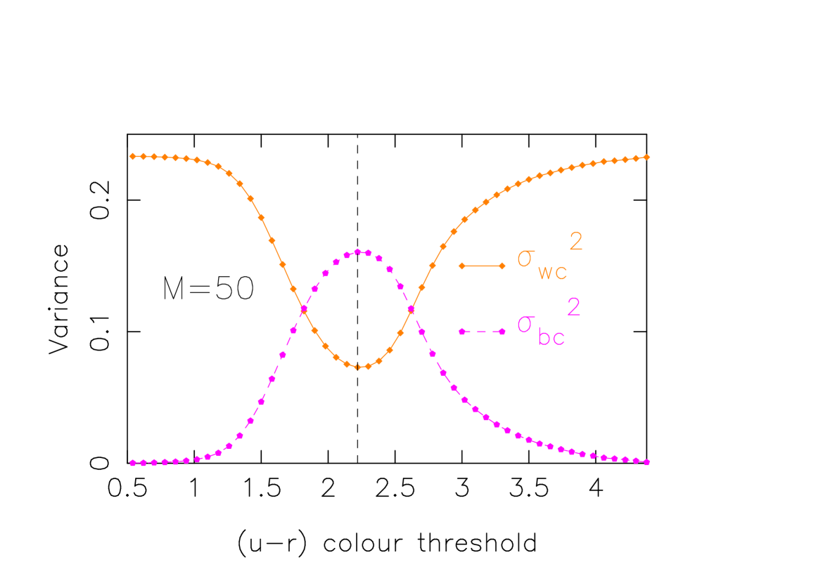
Figure 2: The top left panel shows $P_{B}$ and $P_{R}$ and the top right panel shows $\mu_{B}$ and $\mu_{R}$ as a function of the $(u-r)$ colour threshold. The variances $\sigma_{B}^{2}$, $\sigma_{R}^{2}$ and $\sigma_{wc}^{2}$, $\sigma_{bc}^{2}$ are shown as a function of the $(u-r)$ colour threshold in the bottom left and right panels respectively.

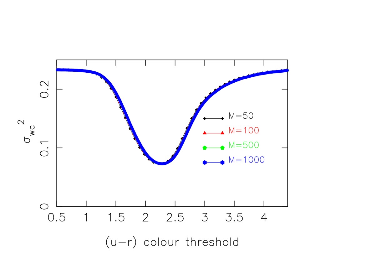
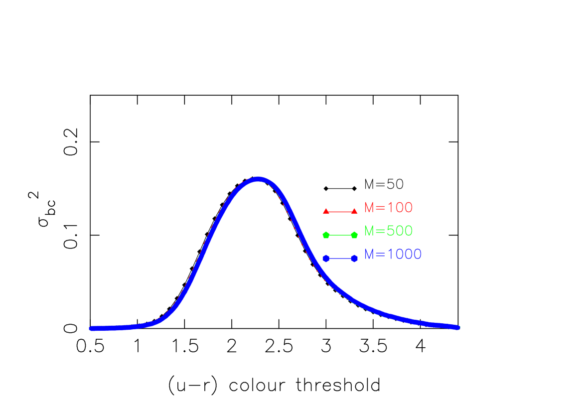
Figure 3: The left panel and the right panel of this figure respectively shows the within-class variance $\sigma_{wc}^{2}$ and the between-class variance $\sigma_{bc}^{2}$ as a function of the $(u-r)$ colour threshold for different choices of the number of bins.

3.1 Implementing Otsu’s thresholding technique to separate the galaxies in the blue cloud and the red sequence

Otsu’s thresholding technique (Otsu, 1979) was originally proposed to separate the foreground pixels from the background pixels in a grayscale image based on their intensities. The pixels with intensities greater than a threshold value are marked as foreground, whereas all pixels with intensity less than or equal to the threshold are labelled as background. It converts the input grayscale image into a binary image. The method iterates through all the possible threshold values and measures the spread of the background and foreground pixels for each threshold. The method aims to find the threshold value for which the ‘intra-class variance’ of the two separate pixel populations is minimum. Interestingly, this maximises the ‘inter-class variance’ of the foreground and background pixels. An optimal threshold that ensures either of these will provide the best separation of the two classes. The method is most efficient when the histogram of the pixel intensities shows a bimodal nature.

The $(u-r)$ colour distribution of the galaxies in the SDSS is strongly bimodal (Strateva, et al., 2001; Balogh, et al., 2004; Baldry, et al., 2004) (Figure 1). It motivates us to use Otsu’s thresholding technique for optimally separating the galaxies in the blue cloud and the red sequence.

We adopt Otsu’s method for this work and outline the primary steps involved in this classification. We consider all the galaxies in our volume limited sample and calculate the histogram of the $(u-r)$ colour using a specific number of bins. We normalize the histogram of the $(u-r)$ colour by the total number of galaxies $N=\sum_{i=1}^{M}n_{i}$ where $n_{i}$ is the number of galaxies in the $i^{th}$ colour bin and $M$ is the total number of bins used in the analysis. This will ensure $\sum_{i=1}^{M}p_{i}=1$ where $p_{i}=\frac{n_{i}}{N}$. The resulting probability distribution can be used to calculate the probabilities of class occurrence for the blue cloud and the red sequence. Let us denote the blue cloud and the reds sequence with $B$ and $R$ respectively. If the threshold corresponds to the $k^{th}$ bin then the bins $[1,....,k]$ belongs to the class $B$ and the class $R$ is represented by the bins $[k+1,....,M]$. The probabilities of the class occurrences for the class $B$ and $R$ can be respectively written as,

$$P_{B}=\sum_{i=1}^{k}p_{i}=w(k)$$ (1)

and

$$P_{R}=\sum_{i=k+1}^{M}p_{i}=1-w(k).$$ (2)

We can use these to calculate the class means for each threshold. They are respectively given by,

$$\mu_{B}=\frac{\sum_{i=1}^{k}c_{i}p_{i}}{P_{B}}=\frac{\mu_{k}}{w(k)}$$ (3)

and

$$\mu_{R}=\frac{\sum_{i=k+1}^{M}c_{i}p_{i}}{P_{R}}=\frac{\mu_{T}-\mu_{k}}{1-w(k)}$$ (4)

where, $c_{i}$ is the $(u-r)$ colour corresponding to the $i^{th}$ bin, $\mu_{k}=\sum_{i=1}^{k}c_{i}p_{i}$ is the mean upto the $k^{th}$ bin and $\mu_{T}=\sum_{i=1}^{M}c_{i}p_{i}$ is the mean of the entire distribution. It may be noted that $P_{B}+P_{R}=1$ and $\mu_{T}=P_{B}\,\mu_{B}+P_{R}\,\mu_{R}$ for each and every threshold.

Similarly, we can also estimate the class variances as,

$$\sigma_{B}^{2}=\frac{\sum_{i=1}^{k}(c_{i}-\mu_{B})^{2}p_{i}}{P_{B}}$$ (5)

and

$$\sigma_{R}^{2}=\frac{\sum_{i=k+1}^{M}(c_{i}-\mu_{R})^{2}p_{i}}{P_{R}}$$ (6)

We can define the classification threshold in two different ways: (i) by minimizing the within-class variance or intra-class variance $\sigma_{wc}^{2}$ or (ii) by maximizing the between-class variance or the inter-class variance $\sigma_{bc}^{2}$.

The within-class variance $\sigma_{wc}^{2}$ and the between-class variance $\sigma_{bc}^{2}$ can be respectively written as,

$$\sigma_{wc}^{2}=P_{B}\,\sigma_{B}^{2}+P_{R}\,\sigma_{R}^{2}$$ (7)

and

$$\sigma_{bc}^{2}=P_{B}\,P_{R}\,(\mu_{B}-\mu_{R})^{2}$$ (8)

The total variance $\sigma_{T}^{2}$ is the sum of the intra-class and inter-class variances,

$$\sigma_{T}^{2}=\sigma_{wc}^{2}+\sigma_{bc}^{2}$$ (9)

It may be noted that both $\sigma_{wc}^{2}$ and $\sigma_{bc}^{2}$ depend on the chosen threshold, but $\sigma_{T}^{2}$ is independent of the threshold. Otsu’s algorithm iteratively searches for the threshold that minimizes the intra-class variance or maximizes the inter-class variance. Fortunately, the threshold that minimizes $\sigma_{wc}^{2}$ also maximizes $\sigma_{bc}^{2}$. So one can choose either Equation 7 or Equation 8 to determine the optimal threshold for the classification. $\sigma_{wc}^{2}$ involves the second-order statistics whereas $\sigma_{bc}^{2}$ is only based on the first-order statistics. Consequently, it is easier to calculate the desired threshold using $\sigma_{bc}^{2}$. In this work, we use both $\sigma_{wc}^{2}$ and $\sigma_{bc}^{2}$ to classify the galaxies in the blue cloud and the red sequence.

Iteration	$\mu_{B}$	$\mu_{R}$	threshold	$|\Delta|$ threshold
1	$1.861672$	$2.681102$	$2.22$
2	$2.074795$	$2.508090$	$2.279581$	$0.059581$
3	$2.188867$	$2.412384$	$2.295775$	$0.016194$
4	$2.244947$	$2.358102$	$2.298391$	$0.002615$
5	$2.273358$	$2.330187$	$2.300393$	$0.002002$
6	$2.287296$	$2.316201$	$2.301204$	$0.000812$

Table 1: This table shows the smaller mean ($\mu_{B}$), the larger mean ($\mu_{R}$), the $(u-r)$ threshold and the absolute difference between two consecutive thresholds ($|\Delta$|) at each iterations of the iterative triclass thresholding method. Here we set a critical $|\Delta|=0.001$ and choose the number of bins to be $50$.

3.2 Iterative triclass thresholding technique: an improved version of Otsu’s method

The primary limitation of Otsu’s method is that the class with the larger variance has a greater influence in determining the classification threshold. It may provide sub-optimal results when one of the classes has a considerably larger variance. Several improvements of the standard Otsu’s method have been proposed in the literature. Here, we have chosen an iterative triclass thresholding technique proposed by Cai et al. (2014).

In this method, we first determine the threshold using the standard Otsu’s algorithm. We then separate the galaxies into three classes based on the mean of the two classes. We define the galaxies in the blue cloud as those with an $(u-r)$ colour less than the smaller mean. The galaxies in the red sequence are defined as those having their $(u-r)$ colour greater than the larger mean. The intervening region between the two means are defined as the "to-be-determined." (TBD) class. In the next iteration, the regions already classified as blue cloud and red sequence are kept unchanged. The standard Otsu’s method is again applied only to the TBD region to divide it into three classes similarly. We get a new threshold after each iteration. The iteration procedure stops when the difference between two consecutive thresholds is less than a preset value. The TBD region is divided into two classes instead of three at the last iteration. Finally, the classified blue cloud is the logical union of all the regions that are previously identified as the blue cloud throughout the different iterations. The final region consisting of the red sequence is determined identically.

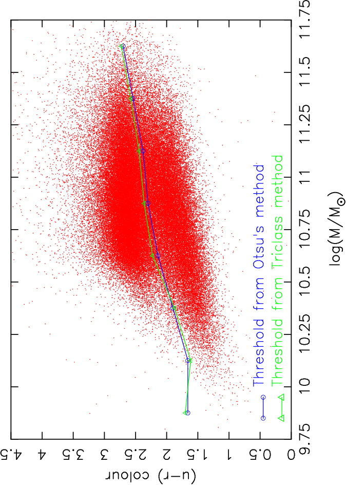
Figure 4: This shows the $(u-r)$ colour thresholds as a function of stellar mass. The dividing lines between the blue cloud and the red sequence are shown together for both the Otsu’s method and the iterative triclass thresholding technique.

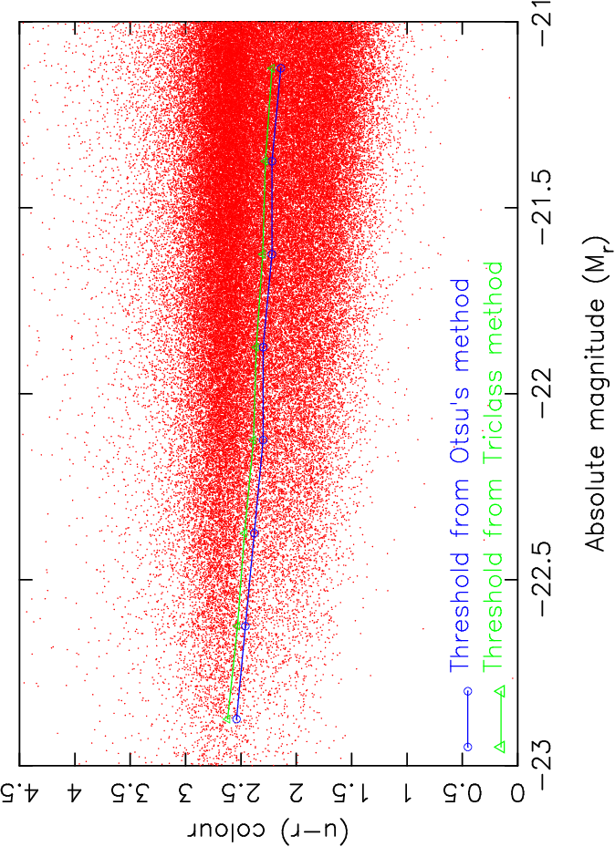
Figure 5: This shows the $(u-r)$ colour thresholds as a function of r-band Absolute magnitude. The boundary lines between the blue cloud and the red sequence are shown together for both the Otsu’s method and the iterative triclass method.

3.3 Results and Conclusions

We show the probability distribution function of the $(u-r)$ colour for the SDSS galaxies in Figure 1. The $(u-r)$ colour distribution clearly shows a bimodal nature that motivates us to use the Otsu’s thresholding technique to classify the two populations associated with the two peaks of the distribution.

We show the probabilities of the class occurrences ( Equation 1 and Equation 2) as a function of the $(u-r)$ colour threshold for the blue cloud and the red sequence in the top left panel of Figure 2. The associated means and variances (Equation 3, Equation 4, Equation 5 and 6) of the two populations as a function of the $(u-r)$ colour threshold are respectively shown in the top right and bottom left panels of Figure 2. We compute the within-class variance $\sigma_{wc}^{2}$ and the between-class variance $\sigma_{bc}^{2}$ of the two populations using Equation 7 and Equation 8. The results are shown in the bottom right panel of Figure 2. We find that the within-class variance $\sigma_{wc}^{2}$ has its minimum at a $(u-r)$ colour threshold of $2.22$. We also note that the between-class variance $\sigma_{bc}^{2}$ has its maximum at $(u-r)=2.22$. Thus $\sigma_{wc}^{2}$ is minimized and $\sigma_{bc}^{2}$ is maximized at exactly the same $(u-r)$ colour threshold.

It may be noted that the results shown in the Figure 1 and Figure 2 correspond to a choice of the number of bins $n=50$. We also test if the locations of the minimum of $\sigma_{wc}^{2}$ and the maximum of $\sigma_{bc}^{2}$ are sensitive to the choice of the number of bins. We repeat our analysis for $n=100$, $500$ and $1000$ and show $\sigma_{wc}^{2}$ and $\sigma_{bc}^{2}$ as a function of the $(u-r)$ colour threshold for four different choices of the number of bins in the left and right panels of Figure 3. Interestingly, the locations of the minimum of $\sigma_{wc}^{2}$ and the maximum of $\sigma_{bc}^{2}$ are independent of the choice of the number of bins. The threshold obtained using this method is insensitive to the choice of binning and thus provides a robust technique for classifying the red and blue galaxies.

We propose Otsu’s technique as a parameter-free method for the automated classification of the galaxies in the blue cloud and the red sequence. It is interesting to note that the $(u-r)$ colour threshold predicted by Otsu’s method in this work matches with the $(u-r)$ colour separator proposed by Strateva, et al. (2001). Strateva, et al. (2001) proposed this as an empirical cut based on the best fit colour-magnitude relations. We also applied the iterative triclass thresholding technique based on Otsu’s method to improve the classification. The threshold values obtained after each iteration in the iterative triclass thresholding scheme are tabulated in Table 1. The iteration is continued until the absolute difference between two consecutive thresholds ($|\Delta|$) is smaller than a preset value. We choose $|\Delta|=10^{-3}$ for the present analysis. It leads to the convergence to an $(u-r)$ colour threshold of $2.301$ after six iterations. We note that the modified version of Otsu’s method is a nearly parameter-free method that can be used effectively for separating red and blue galaxies. It may be noted that the triclass thresholding technique yields a somewhat larger value for the threshold as compared to the Otsu’s method. We know that the differences in the variances of the two classes may bias the classification threshold in the Otsu’s method. The triclass method takes this into account and hence provides an unbiased estimate of the threshold. Further, there exist clear relationships between colour and stellar mass or absolute magnitude. Consequently, a single colour threshold for the galaxies of all masses and luminosity can not be justified. Hence, we divide the entire sample into a number of independent stellar mass bins and separately apply the Otsu’s method and the iterative triclass thresholding technique to each of these stellar mass bins. We show the dividing lines between the blue cloud and the red sequence in the colour-stellar mass plane in Figure 4. A similar analysis is also carried out using a number of absolute magnitude bins. The boundary lines between the two populations in the colour-absolute magnitude plane are shown in Figure 5.

The same dataset has been used earlier to divide the red, green and blue galaxies using a fuzzy set theory based method (Pandey, 2020). This method is also used in an in-depth astronomical study (Das, Pandey, & Sarkar, 2021). The application of a sharp cut would always introduce some contaminations due to the presence of the green valley between the blue cloud and the red sequence. The green valley is populated by transitioning galaxies that evolve from star-forming to quiescent systems. One needs to also identify the green valley in order to separate the blue cloud and the red sequence in an effective manner. Currently, there are no provision for identifying the green valley using Otsu’s method or the triclass thresholding technique used in the present work. Pandey (2020) apply their method to the entire sample without considering the variations of the colour criteria with stellar mass or absolute magnitude. However, we consider these variations in the present work and repeat our analysis in a number of independent stellar mass bins and absolute magnitude bins. This allows us to classify the red and blue populations in the colour-stellar mass plane and colour-absolute magnitude plane. We plan to use the proposed classification scheme in a future in-depth astronomical study.

A caveat in our analysis is that we use observed colour for simplicity. The galaxy colours are affected by the reddening due to redshift and the internal extinction. Ideally, one should use the rest-frame colours for any such classification (Salim, 2014; Taylor et al., 2015).

The distributions of several other galaxy properties, such as the star formation rate, the stellar mass, the bulge to disk mass ratio and the stellar age (Elbaz et al., 2007; Drory, et al., 2009; Driver, et al., 2006; Zibetti et al., 2017) also exhibit a bimodal nature. The galaxies in the red sequence are known to have lower star formation rates and higher stellar masses, higher stellar ages, higher bulge-to-disk mass ratios as compared to the galaxies in the blue cloud. Otsu’s method can be applied to classify the galaxies based on each of these properties. One can employ simultaneous cuts on multiple properties to improve the red-blue classification proposed in this work.

The primary aim of the present work is to find a mathematically justified definition of the red and blue populations in a given data set. We conclude that Otsu’s thresholding technique provides us with a robust and parameter-free method for classifying the galaxies based on the bimodal distributions of galaxy colour.

4 Acknowledgementt

The author thanks the anonymous reviewers for the valuable comments and suggestions. The author would like to acknowledge the financial support from the SERB, DST, Government of India through the project CRG/2019/001110. The author also thanks Suman Sarkar for the help with the SDSS data. Finally, thanks to the SDSS team for making the data public.

References

- Ahumada et al. (2020) Ahumada R., Prieto C. A., Almeida A., Anders F., Anderson S. F., Andrews B. H., Anguiano B., et al., 2020, ApJS, 249, 3
- Arnouts et al. (2013) Arnouts S., Le Floc’h E., Chevallard J., Johnson B. D., Ilbert O., Treyer M., Aussel H., et al., 2013, A&A, 558, A67
- Balogh, et al. (2004) Balogh M. L., Baldry I. K., Nichol R., Miller C., Bower R., Glazebrook K., 2004, ApJL, 615, L101
- Baldry, et al. (2004) Baldry I. K., Glazebrook K., Brinkmann J., Ivezić Ž., Lupton R. H., Nichol R. C., Szalay A. S., 2004, ApJ, 600, 681
- Baldry, et al. (2006) Baldry I. K., Balogh M. L., Bower R. G., Glazebrook K., Nichol R. C., Bamford S. P., Budavari T., 2006, MNRAS, 373, 469
- Bamford et al. (2009) Bamford S. P., Nichol R. C., Baldry I. K., Land K., Lintott C. J., Schawinski K., Slosar A., et al., 2009, MNRAS, 393, 1324
- Bell, et al. (2003) Bell E. F., McIntosh D. H., Katz N., Weinberg M. D., 2003, ApJS, 149, 289
- Bell, et al. (2004) Bell E. F., et al., 2004, ApJ, 608, 752
- Blanton, et al. (2003) Blanton M. R., et al., 2003, ApJ, 594, 186
- Brammer et al. (2009) Brammer G. B., Whitaker K. E., van Dokkum P. G., Marchesini D., Labbé I., Franx M., Kriek M., et al., 2009, ApJL, 706, L173
- Bremer et al. (2018) Bremer M. N., Phillipps S., Kelvin L. S., De Propris R., Kennedy R., Moffett A. J., Bamford S., et al., 2018, MNRAS, 476, 12
- Cai et al. (2014) Cai, H.,Yang, Z., Cao, X., Xia, W., Xu, X.,2014, IEEE Transactions on Image Processing, 23, 1038
- Cattaneo, et al. (2006) Cattaneo A., Dekel A., Devriendt J., Guiderdoni B., Blaizot J., 2006, MNRAS, 370, 1651
- Cattaneo, et al. (2007) Cattaneo A., et al., 2007, MNRAS, 377, 63
- Cameron, et al. (2009) Cameron E., Driver S. P., Graham A. W., Liske J., 2009, ApJ, 699, 105
- Conroy, Gunn & White (2009) Conroy, C., Gunn, J. E., & White, M., 2009, ApJ, 699, 486
- Correa, Schaye & Trayford (2019) Correa C. A., Schaye J., Trayford J. W., 2019, MNRAS, 484, 4401
- Das, Pandey, & Sarkar (2021) Das A., Pandey B., Sarkar S., 2021, JCAP, 2021, 045
- Driver, et al. (2006) Driver S. P., et al., 2006, MNRAS, 368, 414
- Drory, et al. (2009) Drory N., et al., 2009, ApJ, 707, 1595
- Elbaz et al. (2007) Elbaz D., Daddi E., Le Borgne D., Dickinson M., Alexander D. M., Chary R.-R., Starck J.-L., et al., 2007, A&A, 468, 33
- Faber et al. (2007) Faber S. M., Willmer C. N. A., Wolf C., Koo D. C., Weiner B. J., Newman J. A., Im M., et al., 2007, ApJ, 665, 265
- Fritz et al. (2014) Fritz A., Scodeggio M., Ilbert O., Bolzonella M., Davidzon I., Coupon J., Garilli B., et al., 2014, A&A, 563, A92
- Gong et al. (2015) Gong X., Zhong L., Rao R., 2023, A&A, 670, A132
- Holwerda et al. (2022) Holwerda B. W., Smith D., Porter L., Henry C., Porter-Temple R., Cook K., Pimbblet K. A., et al., 2022, MNRAS, 513, 1972
- Hoyle et al. (2002) Hoyle, F., et al. 2002, ApJ, 580, 663
- Kauffmann et al. (2003) Kauffmann G., Heckman T. M., White S. D. M., Charlot S., Tremonti C., Peng E. W., Seibert M., et al., 2003, MNRAS, 341, 54
- Kayo, et al. (2004) Kayo I., et al., 2004, PASJ, 56, 415
- Madau et al. (1996) Madau P., Ferguson H. C., Dickinson M. E., Giavalisco M., Steidel C. C., Fruchter A., 1996, MNRAS, 283, 1388
- Menci, et al. (2005) Menci N., Fontana A., Giallongo E., Salimbeni S., 2005, ApJ, 632, 49
- Nelson, et al. (2018) Nelson D., et al., 2018, MNRAS, 475, 624
- Otsu (1979) Otsu, N., 1979, IEEE Transactions on Systems, Man, and Cybernetics, 9, 62
- Pandey & Bharadwaj (2006) Pandey, B., Bharadwaj, S. 2006, MNRAS, 372, 827
- Pandey & Sarkar (2020) Pandey B., Sarkar S., 2020, MNRAS, 498, 6069
- Pandey (2020) Pandey B., 2020, MNRAS, 499, L31
- Planck Collaboration, et al. (2018) Planck Collaboration, et al., 2018, arXiv, arXiv:1807.06209
- Salim (2014) Salim S., 2014, Serbian Astronomical Journal, 189, 1
- Strateva, et al. (2001) Strateva I., et al., 2001, AJ, 122, 1861
- Taylor et al. (2015) Taylor E. N., Hopkins A. M., Baldry I. K., Bland-Hawthorn J., Brown M. J. I., Colless M., Driver S., et al., 2015, MNRAS, 446, 2144
- Trayford et al. (2016) Trayford, J. W. et al., 2016, MNRAS, 460, 3925
- Turner et al. (2019) Turner S., Kelvin L. S., Baldry I. K., Lisboa P. J., Longmore S. N., Collins C. A., Holwerda B. W., et al., 2019, MNRAS, 482, 126
- Williams et al. (2009) Williams R. J., Quadri R. F., Franx M., van Dokkum P., Labbé I., 2009, ApJ, 691, 1879
- York et al. (2000) York, D. G., et al. 2000, AJ, 120, 1579
- Zehavi, et al. (2011) Zehavi I., et al., 2011, ApJ, 736, 59
- Zheng et al. (2015) Zheng C., Pulido J., Thorman P., Hamann B., 2015, MNRAS, 451, 4445
- Zibetti et al. (2017) Zibetti S., Gallazzi A. R., Ascasibar Y., Charlot S., Galbany L., García Benito R., Kehrig C., et al., 2017, MNRAS, 468, 1902