Convergence Analyses of Davis–Yin Splitting via Scaled Relative Graphs II:
Convex Optimization Problems

Abstract

The prior work of [arXiv:2207.04015, 2022] used scaled relative graphs (SRG) to analyze the convergence of Davis–Yin splitting (DYS) iterations on monotone inclusion problems. In this work, we use this machinery to analyze DYS iterations on convex optimization problems and obtain state-of-the-art linear convergence rates.

[label1] organization=Seoul National University, Department of mathematical sciences, addressline=1 Gwanak-ro, Gwanak-gu, city=Seoul, postcode=08826, country=Korea

1 Introduction

Consider the problem

$$\begin{array}[]{ll}\underset{x\in{\mathcal{H}}}{\mbox{minimize}}&f(x)+g(x)+h(x),\end{array}$$ (1)

where ${\mathcal{H}}$ is a Hilbert space, $f$, $g$, and $h$ are convex, closed, and proper functions, and $h$ is differentiable with $L$-Lipschitz continuous gradients. The Davis–Yin splitting (DYS) [1] solves this problem by performing the fixed-point iteration with

$${\varbbT}={\varbbI}-\mathrm{Prox}_{\alpha g}+\mathrm{Prox}_{\alpha f}(2\mathrm{Prox}_{\alpha g}-{\varbbI}-\alpha\nabla h\mathrm{Prox}_{\alpha g}),$$ (2)

where $\alpha>0$, $\mathrm{Prox}_{\alpha f}$ and $\mathrm{Prox}_{\alpha g}$ are the proximal operators with respect to $\alpha f$ and $\alpha g$, and is the identity mapping. DYS has been used as a building block for various algorithms for a diverse range of optimization problems [2, 3, 4, 5, 6, 7].

Much prior work has been dedicated to analyzing the convergence rate of DYS iterations [1, 8, 9, 10, 11, 12, 13]. Recently, Lee, Yi, and Ryu [14] leveraged the recently introduced scaled relative graphs (SRG) [15] to obtain tighter analyses. However, the focus of [14] was on DYS applied to general class monotone operators, rather than the narrower class of subdifferential operators.

In this paper, we use the SRG theory of [14] to analyze the linear convergence rates of DYS applied to convex optimization problems and obtain state-of-the-art rates.

1.1 Prior works

For explaining and inducing many convex optimization algorithms, splitting methods for monotone inclusion problems has been a potent tool[16, 17, 18]. Renowned examples of this methodology include forward-backward splitting (FBS) [19, 20], Douglas–Rachford splitting (DRS) [21, 22, 23], and alternating directions method of multipliers (ADMM) [24], which have been widely used in application regimes. While FBS and DRS are concerned with the sum of two monotone operators, Davis and Yin proposed a new splitting method for the sum of three monotone operators [1], thereby uniting the aforementioned methods. This has come up with a variety of applications [2, 3, 4, 5, 6, 7] and many variants, including stochastic DYS [25, 26, 27, 28, 29], inexact DYS [30], adaptive DYS [31], inertial DYS [32], and primal-dual DYS[33].

Compared to the substantial amount of these studies on DYS, there is not much literature on linear convergence analysis of the DYS iteration. One approach is to formulate SDPs that numerically find the tight contraction factors of DYS: Ryu, Taylor, Bergeling, and Giselsson [11] and Wang, Fazlyab, Chen, and Preciado [12] carried out this approach using the performance estimation problem (PEP) and integral quadratic constraint (IQC), respectively. However, this approach does not give an analytical expression of the contraction factors. There is far less literature that gives an analytical expression of the contraction factors. Two of them are respectively done by Davis and Yin [1], and Condat and Richtarik [13] via inequality analysis. On the other hand, Lee, Yi, and Ryu [14] made a different approach utilizing scaled relative graphs.

This novel tool, the scaled relative graphs (SRG) [15], renders a new approach to analyzing the behavior of multi-valued operators (in particular, including nonlinear operators) by mapping them to the extended complex plane. This theory was further studied by Huang, Ryu, and Yin [34], where they identified the SRG of normal matrices. Furthermore, Pates leveraged the Toeplitz–Hausdorff theorem to identify SRGs of linear operators [35]. This approach has also been used for analyzing nonlinear operators. To prove the tightness of the averaged coefficient of the composition of averaged operators [36] and the DYS operator [1], Huang, Ryu, and Yin performed analyses of SRGs of those operators [37]. Moreover, there is certain literature on applying SRG to control theory. SRGs have been leveraged by Chaffey, Forni, and Rodolphe to examine input-output properties of feedback systems [38, 39]. Chaffey and Sepulchre have further found its application to characterize behaviors of a given model by leveraging it as an experimental tool [40, 41, 42].

1.2 Preliminaries

Multi-valued operators.

In general, we follow notations regarding multi-valued operators as in [16, 18]. Write ${\mathcal{H}}$ for a real Hilbert space with inner product $\langle\cdot,\cdot\rangle$ and norm $\lVert\cdot\rVert$. To represent that is a multi-valued operator defined on ${\mathcal{H}}$, write ${\varbbA}\colon{\mathcal{H}}\rightrightarrows{\mathcal{H}}$, and define its domain as $\mathrm{dom}\,{\varbbA}=\left\{x\in{\mathcal{H}}\,|\,{\varbbA}x\neq\emptyset\right\}$. We say is single-valued if all outputs of are singletons or the empty set, and identify with the function from $\mathrm{dom}\,{\varbbA}$ to ${\mathcal{H}}$. Define the graph of an operator as

$$\mathrm{graph}({\varbbA})=\{(x,u)\in{\mathcal{H}}\times{\mathcal{H}}\,|\,u\in{\varbbA}x\}.$$

We do not distinguish and $\mathrm{graph}({\varbbA})$ for the sake of notational simplicity. For instance, it is valid to write $(x,u)\in{\varbbA}$ to mean $u\in{\varbbA}x$. Define the inverse of as

$${}^{-1}=\{(u,x)\,|\,(x,u)\in{\varbbA}\},$$

scalar multiplication with an operator as

$$\alpha{\varbbA}=\{(x,\alpha u)\,|\,(x,u)\in{\varbbA}\},$$

the identity operator as

$${\varbbI}=\{(x,x)\,|\,x\in{\mathcal{H}}\},$$

and

$${\varbbI}+\alpha{\varbbA}=\{(x,x+\alpha u)\,|\,(x,u)\in{\varbbA}\}$$

for any $\alpha\in\mathbb{R}$. Define the resolvent of with stepsize $\alpha>0$ as

$${}_{\alpha{\varbbA}}=({\varbbI}+\alpha{\varbbA})^{-1}.$$

Note that _α is a single-valued operator if is monotone, or equivalently if $\langle x-y,u-v\rangle\geq 0$ for all $(x,u)$, $(y,v)\in{\varbbA}$. Define addition and composition of operators ${\varbbA}\colon{\mathcal{H}}\rightrightarrows{\mathcal{H}}$ and ${\varbbB}\colon{\mathcal{H}}\rightrightarrows{\mathcal{H}}$ as

$${\varbbA}+{\varbbB} =\left\{(x,u+v)\,|\,(x,u)\in{\varbbA},(x,v)\in{\varbbB}\right\},$$

$$=\left\{(x,s)\,|\,\exists\,u\;\text{such that}\;(x,u)\in{\varbbB},(u,s)\in{\varbbA}\right\}.$$

We call ${\mathcal{A}}$ a class of operators if it is a set of operators. For any real scalar $\alpha\in\mathbb{R}$, define

$$\alpha{\mathcal{A}}=\{\alpha{\varbbA}\,|\,{\varbbA}\in{\mathcal{A}}\}$$

and

$${\varbbI}+\alpha{\mathcal{A}}=\{{\varbbI}+\alpha{\varbbA}\,|\,{\varbbA}\in{\mathcal{A}}\}.$$

Define

$${\mathcal{A}}^{-1}=\{{}^{-1}\,|\,{\varbbA}\in{\mathcal{A}}\}$$

and ${}_{\alpha{\mathcal{A}}}=({\varbbI}+\alpha{\mathcal{A}})^{-1}$ for $\alpha>0$.

Subdifferential operators.

Unless otherwise stated, functions defined on ${\mathcal{H}}$ are extended real-valued, which means

$$f\colon{\mathcal{H}}\to\mathbb{R}\cup\left\{\pm\infty\right\}.$$

For a function $f$, we define the subdifferential operator $\partial f$ via

$$\partial f(x)=\left\{g\in{\mathcal{H}}\,|\,f(y)\geq f(x)+\langle g,y-x\rangle,\forall y\in{\mathcal{H}}\right\}$$

(we allow $\infty\geq\infty$ and $-\infty\geq-\infty$). In some cases, the subdifferential operator $\partial f$ is a single-valued operator. Then, we write $\nabla f=\partial f$.

Proximal operators.

We call $f$ a CCP function if it is a convex, closed, and proper [18, 16]. For a CCP function $f\colon{\mathcal{H}}\to\mathbb{R}\cup\left\{\pm\infty\right\}$ and $\alpha>0$, we define the proximal operator with respect to $\alpha f$ as

$$\mathrm{Prox}_{\alpha f}(x)=\operatorname*{argmin}_{y\in{\mathcal{H}}}\left\{\alpha f(y)+\frac{1}{2}\lVert x-y\rVert^{2}\right\}.$$

Then, ${}_{\alpha\partial f}=\mathrm{Prox}_{\alpha f}$.

Class of functions and subdifferential operators.

Define $f\colon{\mathcal{H}}\to\mathbb{R}\cup\left\{\pm\infty\right\}$ being $\mu$-strongly convex (for $\mu\in(0,\infty)$) and $L$-smooth (for $L\in(0,\infty)$) as they are defined in [43]. Write

$${\mathcal{F}}_{\mu,L}=\left\{f\,|\,f\text{ is }\mu\text{-strongly convex, }L\text{-smooth, and CCP.}\right\}.$$

for collection of functions that are $\mu$-strongly convex and $L$-smooth at the same time. For notational simplicity, we extend ${\mathcal{F}}_{\mu,L}$ to allow $\mu=0$ or $L=\infty$ by defining

$${\mathcal{F}}_{0,L} =\left\{f\,|\,f\text{ is }L\text{-smooth and CCP.}\right\},$$

$${\mathcal{F}}_{\mu,\infty} =\left\{f\,|\,f\text{ is }\mu\text{-strongly convex and CCP.}\right\},$$

$${\mathcal{F}}_{0,\infty} =\left\{f\,|\,f\text{ is CCP.}\right\}.$$

for $\mu$, $L\in(0,\infty)$.

Subdifferential operators of any functions in ${\mathcal{F}}_{\mu,L}$ are denoted

$$\partial{\mathcal{F}}_{\mu,L}=\left\{\partial f\,|\,f\in{\mathcal{F}}_{\mu,L}\right\}.$$

Complex set notations.

Denote $\overline{\mathbb{C}}=\mathbb{C}\cup\left\{\infty\right\}$, and define $0^{-1}=\infty$ and $\infty^{-1}=0$ in $\overline{\mathbb{C}}$. For $A\subset\overline{\mathbb{C}}$ and $\alpha\in\mathbb{C}$, define

$$\alpha A=\left\{\alpha z\,|\,z\in A\right\},\quad\alpha+A=\left\{\alpha+z\,|\,z\in A\right\},\quad A^{-1}=\left\{z^{-1}\,|\,z\in A\right\}.$$

For $A\subseteq\mathbb{C}$, define the boundary of $A$

$$\partial A=\overline{A}\setminus\mathrm{int}A.$$

We clarify that the usage of $\partial$ operator is different when it is applied to a function or a complex set; the former is the subdifferential operator, and the latter is the boundary operator. For circles and disks on the complex plane, write

$${\mathrm{Circ}}(z,r)=\{w\in\mathbb{C}\,|\,\lvert w-z\rvert=r\},\qquad{\mathrm{Disk}}(z,r)=\{w\in\mathbb{C}\,|\,\lvert w-z\rvert\leq r\}$$

for $z\in\mathbb{C}$ and $r\in(0,\infty)$. Note, ${\mathrm{Circ}}(z,r)=\partial{\mathrm{Disk}}(z,r)$.

Scaled relative graphs [15].

Define the SRG of an operator ${\varbbA}\colon{\mathcal{H}}\rightrightarrows{\mathcal{H}}$ as

$$\mathcal{G}({\varbbA}) =\left\{\frac{\|u-v\|}{\|x-y\|}\exp\left[\pm i\angle(u-v,x-y)\right]\,\Big{|}\,u\in{\varbbA}x,\,v\in{\varbbA}y,\,x\neq y\right\}$$

$$\qquad\qquad\qquad\qquad\qquad\qquad\qquad\bigg{(}\cup\{\infty\}\text{ if ${\varbbA}$ is not single-valued}\bigg{)}.$$

where the angle between $x\in{\mathcal{H}}$ and $y\in{\mathcal{H}}$ is defined as

$$\angle(x,y)=\left\{\begin{array}[]{ll}\arccos\left({\tfrac{\langle x,y\rangle}{\lVert x\rVert\lVert y\rVert}}\right)&\text{ if }x\neq 0,\,y\neq 0\\ 0&\text{ otherwise.}\end{array}\right.$$

Note, SRG is a subset of $\overline{\mathbb{C}}$. Define the SRG of a class of operators ${\mathcal{A}}$ as

$$\mathcal{G}({\mathcal{A}})=\bigcup_{{\varbbA}\in{\mathcal{A}}}\mathcal{G}({\varbbA}).$$

Say ${\mathcal{A}}$ is SRG-full if

$${\varbbA}\in{\mathcal{A}}\quad\Leftrightarrow\quad{\mathcal{G}}({\varbbA})\subseteq{\mathcal{G}}({\mathcal{A}}).$$

Fact 1 (Theorem 4, 5 [15]).

If ${\mathcal{A}}$ is a class of operators, then

$${\mathcal{G}}(\alpha{\mathcal{A}})=\alpha{\mathcal{G}}({\mathcal{A}}),\quad{\mathcal{G}}({\varbbI}+{\mathcal{A}})=1+{\mathcal{G}}({\mathcal{A}}),\quad{\mathcal{G}}({\mathcal{A}}^{-1})={\mathcal{G}}({\mathcal{A}})^{-1}.$$

where $\alpha$ is a nonzero real number. If ${\mathcal{A}}$ is furthermore SRG-full, then $\alpha{\mathcal{A}},{\varbbI}+{\mathcal{A}}$, and ${\mathcal{A}}^{-1}$ are SRG-full.

Fact 2 (Proposition 2 [15]).

Let $0<\mu<L<\infty$. Then

​​​​​​

​​​​​​​​​​​​​​​

​​​​​​​​​​​​​​​​​​

​​​​​​​​​​​​

DYS operators.

Let

_,,,α,λ $$={\varbbI}-\lambda{}_{\alpha{\varbbB}}+\lambda{}_{\alpha{\varbbA}}(2{}_{\alpha{\varbbB}}-{\varbbI}-\alpha{\varbbC}{}_{\alpha{\varbbB}})$$

be the DYS operator for operators ${\varbbA}\colon{\mathcal{H}}\rightrightarrows{\mathcal{H}}$, ${\varbbB}\colon{\mathcal{H}}\rightrightarrows{\mathcal{H}}$, and ${\varbbC}\colon{\mathcal{H}}\rightrightarrows{\mathcal{H}}$ with stepsize $\alpha\in(0,\infty)$ and averaging parameter $\lambda\in(0,\infty)$. In this paper, we usually take ${\varbbA}=\partial f$, ${\varbbB}=\partial g$, and ${\varbbC}=\nabla h$ for some CCP functions $f$, $g$, and $h$ defined on ${\mathcal{H}}$, to obtain

$${}_{\partial f,\partial g,\nabla h,\alpha,\lambda}={\varbbI}-\lambda\mathrm{Prox}_{\alpha g}+\lambda\mathrm{Prox}_{\alpha f}(2\mathrm{Prox}_{\alpha g}-{\varbbI}-\alpha\nabla h\mathrm{Prox}_{\alpha g})$$

what we call the subdifferential DYS operator.

Let

$${}_{{\mathcal{A}},{\mathcal{B}},{\mathcal{C}},\alpha,\lambda}=\left\{{}_{{\varbbA},{\varbbB},{\varbbC},\alpha,\lambda}\,|\,{\varbbA}\in{\mathcal{A}},{\varbbB}\in{\mathcal{B}},{\varbbC}\in{\mathcal{C}}\right\}$$

be the class of DYS operators for operator classes ${\mathcal{A}}$, ${\mathcal{B}}$, and ${\mathcal{C}}$ with $\alpha,\lambda\in(0,\infty)$. Define

$$\zeta_{\text{DYS}}(z_{A},z_{B},z_{C};\alpha,\lambda) =1-\lambda z_{B}+\lambda z_{A}(2z_{B}-1-\alpha z_{C}z_{B})$$

$$=1-\lambda z_{A}-\lambda z_{B}+\lambda(2-\alpha z_{C})z_{A}z_{B},$$

which exhibits symmetry with respect to $z_{A}$ and $z_{B}$, and

$${\mathcal{Z}}^{\text{DYS}}_{{\mathcal{A}},{\mathcal{B}},{\mathcal{C}},\alpha,\lambda}=\left\{\zeta_{\text{DYS}}(z_{A},z_{B},z_{C};\alpha,\lambda)\,|\,z_{A}\in{\mathcal{G}}\left({}_{\alpha{\mathcal{A}}}\right),z_{B}\in{\mathcal{G}}\left({}_{\alpha{\mathcal{B}}}\right),z_{C}\in{\mathcal{G}}\left({\mathcal{C}}\right)\right\}$$

for operator classes ${\mathcal{A}}$, ${\mathcal{B}}$, and ${\mathcal{C}}$ with $\alpha,\lambda\in(0,\infty)$.

Identifying the tight Lipschitz coefficient via SRG.

Say a subset of $\overline{\mathbb{C}}$ is a generalized disk if it is a disk, $\{z\,|\,\operatorname{Re}z\geq a\}\cup\{\infty\}$, or $\{z\,|\,\operatorname{Re}z\leq a\}\cup\{\infty\}$ for a real number $a$. The following is the key fact for calculating the Lipschitz coefficients of the DYS operators via SRG.

Fact 3 (Corollary 1 of [14]).

Let $\alpha,\lambda>0$. Let ${\mathcal{A}}$ and ${\mathcal{B}}$ be SRG-full classes of monotone operators where ${\mathcal{G}}\left({\varbbI}+\alpha{\mathcal{A}}\right)$ forms a generalized disk. Let ${\mathcal{C}}$ be an SRG-full class of single-valued operators. Assume ${\mathcal{G}}\left({\mathcal{A}}\right)$, ${\mathcal{G}}\left({\mathcal{B}}\right)$, and ${\mathcal{G}}\left({\mathcal{C}}\right)$ are nonempty. Then,

$$\sup_{\begin{subarray}{c}{\varbbT}\in{}_{{\mathcal{A}},{\mathcal{B}},{\mathcal{C}},\alpha,\lambda}\\ x,y\in\mathrm{dom}\,{\varbbT},x\neq y\end{subarray}}\frac{\lVert{\varbbT}x-{\varbbT}y\rVert}{\lVert x-y\rVert}=\sup_{z\in{\mathcal{Z}}^{\text{DYS}}_{{\mathcal{A}},{\mathcal{B}},{\mathcal{C}},\alpha,\lambda}}\lvert z\rvert.$$

Indeed, the original version of Fact 3 is consistent with ${\mathcal{G}}\left({\varbbI}+\alpha{\mathcal{A}}\right)$ having a more general property, namely an arc property. We can calculate bounds for the right-hand-side of the equality in Fact 3 efficiently by using the following fact.

Fact 4 (Lemma 1 of [14]).

Let $f\colon\mathbb{C}^{3}\to\mathbb{C}$ be a polynomial of three complex variables. Let $A$, $B$, and $C$ be compact subsets of $\,\mathbb{C}$. Then,

$$\max_{\begin{subarray}{c}z_{A}\in A,z_{B}\in B,\\ z_{C}\in C\end{subarray}}\lvert f(z_{A},z_{B},z_{C})\rvert=\max_{\begin{subarray}{c}z_{A}\in\partial A,z_{B}\in\partial B,\\ z_{C}\in\partial C\end{subarray}}\lvert f(z_{A},z_{B},z_{C})\rvert.$$

2 Lipschitz factors of subdifferential DYS

We present Lipschitz factors of subdifferential DYS operators. To the best of our knowledge, the following results are the best linear convergence rates of the DYS iteration compared to Theorem 9 of [13] and Theorems 3, 4, and 5 of [14]. To clarify, our rates are not slower than the prior rates in all cases and faster in most cases.

Theorem 1.

Let $f\in{\mathcal{F}}_{\mu_{f},L_{f}}$, $g\in{\mathcal{F}}_{\mu_{g},L_{g}}$, and $h\in{\mathcal{F}}_{\mu_{h},L_{h}}$, where

$$0\leq\mu_{f}<L_{f}\leq\infty,\quad 0\leq\mu_{g}<L_{g}\leq\infty,\quad 0\leq\mu_{h}<L_{h}<\infty.$$

Let $\lambda>0$ be an averaging parameter and $\alpha>0$ be a step size. Throughout this theorem, define $r/\infty=0$ for any real number $r$. Write

$$C_{f}=\frac{1}{2}\left(\frac{1}{1+\alpha\mu_{f}}+\frac{1}{1+\alpha L_{f}}\right),\quad C_{g}=\frac{1}{2}\left(\frac{1}{1+\alpha\mu_{g}}+\frac{1}{1+\alpha L_{g}}\right),$$

$$R_{f}=\frac{1}{2}\left(\frac{1}{1+\alpha\mu_{f}}-\frac{1}{1+\alpha L_{f}}\right),\quad R_{g}=\frac{1}{2}\left(\frac{1}{1+\alpha\mu_{g}}-\frac{1}{1+\alpha L_{g}}\right),$$

$$d=\max\{\lvert 2-\lambda-\alpha\mu_{h}\rvert,\lvert 2-\lambda-\alpha L_{h}\rvert\}.$$

If $\lambda<1/C_{f}$, then _{∂f,∂g,∇h,α,λ} is $\rho_{f}$-Lipschitz, where

$$\rho_{f}^{2}=\left(1-\lambda\frac{C_{f}^{2}-R_{f}^{2}}{C_{f}}\right)\max\bigg{\{}\left(1-\frac{\lambda}{1+\alpha\mu_{g}}\right)^{2}+\frac{\lambda d^{2}}{1/C_{f}-\lambda}\left(\frac{1}{1+\alpha\mu_{g}}\right)^{2},$$

$$\qquad\qquad\qquad\qquad\qquad\qquad\quad\left(1-\frac{\lambda}{1+\alpha L_{g}}\right)^{2}+\frac{\lambda d^{2}}{1/C_{f}-\lambda}\left(\frac{1}{1+\alpha L_{g}}\right)^{2}\bigg{\}}.$$

Symmetrically, if $\lambda<1/C_{g}$, then _{∂f,∂g,∇h,α,λ} is $\rho_{g}$-Lipschitz, where

$$\rho_{g}^{2}=\left(1-\lambda\frac{C_{g}^{2}-R_{g}^{2}}{C_{g}}\right)\max\bigg{\{}\left(1-\frac{\lambda}{1+\alpha\mu_{f}}\right)^{2}+\frac{\lambda d^{2}}{1/C_{g}-\lambda}\left(\frac{1}{1+\alpha\mu_{f}}\right)^{2},$$

$$\qquad\qquad\qquad\qquad\qquad\qquad\quad\left(1-\frac{\lambda}{1+\alpha L_{f}}\right)^{2}+\frac{\lambda d^{2}}{1/C_{g}-\lambda}\left(\frac{1}{1+\alpha L_{f}}\right)^{2}\bigg{\}}.$$

Theorem 2.

Let $f$, $g$, $h$, $\mu_{f}$, $L_{f}$, $\mu_{g}$, $L_{g}$, $\mu_{h}$, $L_{h}$, $\lambda$, and $\alpha$ be the same as in Theorem 1. Additionally, assume $\lambda<2-\frac{\alpha(\mu_{h}+L_{h})}{2}$. Define $\infty/\infty^{2}=0$. Write

$$\nu_{f}=\min\left\{\frac{2\mu_{f}+\mu_{h}}{(1+\alpha\mu_{f})^{2}},\frac{2L_{f}+\mu_{h}}{(1+\alpha L_{f})^{2}}\right\},\quad\nu_{g}=\min\left\{\frac{2\mu_{g}+\mu_{h}}{(1+\alpha\mu_{g})^{2}},\frac{2L_{g}+\mu_{h}}{(1+\alpha L_{g})^{2}}\right\},$$

$$\theta=\frac{2}{4-\alpha(\mu_{h}+L_{h})}.$$

Then, _{∂f,∂g,∇h,α,λ} is $\rho$-contractive, where

$$\rho^{2}=1-\lambda\theta+\lambda\sqrt{\left(\theta-\alpha\nu_{f}\right)\left(\theta-\alpha\nu_{g}\right)}.$$

2.1 Proofs of Theorems 1 and 2

To leverage Fact 3, we need to set adequate SRG-full operator classes ${\mathcal{A}}$, ${\mathcal{B}}$, and ${\mathcal{C}}$ to apply it. The most natural choice is to set

$${\mathcal{A}}=\partial{\mathcal{F}}_{\mu_{f},L_{f}},\quad{\mathcal{B}}=\partial{\mathcal{F}}_{\mu_{g},L_{g}},\quad{\mathcal{C}}=\partial{\mathcal{F}}_{\mu_{h},L_{h}}.$$

However, this choice is not appropriate since these are not SRG-full classes. To overcome this issue, we introduce the following operator classes:

$${\mathcal{D}}_{f} =\{{\varbbA}\colon{\mathcal{H}}\rightrightarrows{\mathcal{H}}\,|\,{\mathcal{G}}({\varbbA})\subseteq{\mathcal{G}}(\partial{\mathcal{F}}_{\mu_{f},L_{f}})\},$$

$${\mathcal{D}}_{g} =\{{\varbbB}\colon{\mathcal{H}}\rightrightarrows{\mathcal{H}}\,|\,{\mathcal{G}}({\varbbB})\subseteq{\mathcal{G}}(\partial{\mathcal{F}}_{\mu_{g},L_{g}})\},$$

$${\mathcal{D}}_{h} =\{{\varbbC}\colon{\mathcal{H}}\rightrightarrows{\mathcal{H}}\,|\,{\mathcal{G}}({\varbbC})\subseteq{\mathcal{G}}(\partial{\mathcal{F}}_{\mu_{h},L_{h}})\}.$$

To elaborate, we gather all operators that have its SRG within ${\mathcal{G}}(\partial{\mathcal{F}}_{\mu_{f},L_{f}})$ to form ${\mathcal{D}}_{f}$, and so on. Then, ${\mathcal{D}}_{f}$, ${\mathcal{D}}_{g}$, and ${\mathcal{D}}_{h}$ are SRG-full classes by definition. We now consider ${\mathcal{A}}={\mathcal{D}}_{f}$, ${\mathcal{B}}={\mathcal{D}}_{g}$, and ${\mathcal{C}}={\mathcal{D}}_{h}$ in the following proof.

We mention two elementary facts.

Fact 5.

For $a,b,c,d\in[0,\infty)$,

$$\left(\sqrt{ab}+\sqrt{cd}\right)^{2}\leq(a+c)(b+d).$$

Proof.

This inequality is an instance of Cauchy–Schwartz. ∎

Fact 6.

Let $k$, $l$, and $r$ be positive real numbers, and $b$, $c$ be a real number. For $z\in{\mathrm{Circ}}(c,r)$,

$$k\lvert z-b\rvert^{2}+l\lvert z\rvert^{2}$$

is maximized at $z=c-r$ or $z=c+r$.

Proof to Fact 6.

Observe that

$$k\lvert z-b\rvert^{2}+l\lvert z\rvert^{2}=(k+l)\left|z-\frac{kb}{k+l}\right|^{2}+\frac{klb^{2}}{k+l}.$$

and distance from $\frac{kb}{k+l}$ to $z\in{\mathrm{Circ}}(c,r)$ is maximized at $z=c-r$ if $\frac{kb}{k+l}>c$ and $z=c+r$ otherwise. ∎

We now prove Theorem 1, 2. We use the similar proof technique introduced in the previous work [14].

Proof to Theorem 1.

We first prove the first statement and show the other by the same reasoning. Invoking Fact 3 and Fact 4, it suffices to show that

$$\lvert\zeta_{\text{DYS}}(z_{f},z_{g},z_{h};\alpha,\lambda)\rvert^{2}\leq\rho_{f}^{2}$$

for

$$z_{f} \in\partial{\mathcal{G}}\left({}_{\alpha{\mathcal{D}}_{f}}\right)={\mathrm{Circ}}\left(C_{f},R_{f}\right),$$

$$z_{g} \in\partial{\mathcal{G}}\left({}_{\alpha{\mathcal{D}}_{g}}\right)={\mathrm{Circ}}\left(C_{g},R_{g}\right),$$

$$z_{h} \in\partial{\mathcal{G}}\left({\mathcal{D}}_{h}\right)={\mathrm{Circ}}\left(\frac{L_{h}+\mu_{h}}{2},\frac{L_{h}-\mu_{h}}{2}\right)$$

(refer to Fact 2 and Fact 1 to see why $\partial{\mathcal{G}}\left({}_{\alpha{\mathcal{D}}_{f}}\right)$, $\partial{\mathcal{G}}\left({}_{\alpha{\mathcal{D}}_{g}}\right)$, ${\mathcal{G}}\left({\mathcal{D}}_{h}\right)$ are formed correspondingly) when $\lambda<1/C_{f}$ holds.

Define

$$r=\frac{d}{1/C_{f}-\lambda}.$$

Then,

$$\lvert\zeta_{\text{DYS}}(z_{f},z_{g},z_{h};\alpha,\lambda)\rvert^{2} =\lvert 1-\lambda z_{f}-\lambda z_{g}+\lambda(2-\alpha z_{h})z_{f}z_{g}\rvert^{2}$$

$$=\lvert(1-\lambda z_{f})(1-\lambda z_{g})+\lambda(2-\lambda-\alpha z_{h})z_{f}z_{g}\rvert^{2}$$

$$\leq\left(\lvert(1-\lambda z_{f})(1-\lambda z_{g})\rvert+\lvert\lambda(2-\lambda-\alpha z_{h})z_{f}z_{g}\rvert\right)^{2}$$

$$\stackrel{{\scriptstyle(i)}}{{\leq}}\left(\lvert(1-\lambda z_{f})(1-\lambda z_{g})\rvert+\lambda d\lvert z_{f}z_{g}\rvert\right)^{2}$$

$$\stackrel{{\scriptstyle(ii)}}{{\leq}}\left(\lvert 1-\lambda z_{f}\rvert^{2}+\lambda dr^{-1}\lvert z_{f}\rvert^{2}\right)\left(\lvert 1-\lambda z_{g}\rvert^{2}+\lambda dr\lvert z_{g}\rvert^{2}\right).$$ (3)

We have used $\lvert 2-\lambda-\alpha z_{h}\rvert\leq\max\{\lvert 2-\lambda-\alpha\mu_{h}\rvert,\lvert 2-\lambda-\alpha L_{h}\rvert\}=d$ in $(i)$ and Fact 5 in $(ii)$.

Recall that $\partial{\mathcal{G}}\left({}_{\alpha{\mathcal{D}}_{f}}\right)={\mathrm{Circ}}(C_{f},R_{f})$. This renders

$$\lvert 1-\lambda z_{f}\rvert^{2}+\lambda dr^{-1}\lvert z_{f}\rvert^{2}=\frac{\lambda}{C_{f}}\lvert z_{f}-C_{f}\rvert^{2}+1-\lambda C_{f}=1-\lambda\frac{C_{f}^{2}-R_{f}^{2}}{C_{f}}.$$ (4)

For the latter term, $z_{g}=\frac{1}{1+\alpha\mu_{g}}$ or $z_{g}=\frac{1}{1+\alpha L_{g}}$ give the maximum, invoking Fact 6. Therefore,

$$\lvert 1-\lambda z_{g}\rvert^{2}+\lambda dr\lvert z_{g}\rvert^{2}$$

$$\leq\max\bigg{\{}\left(1-\frac{\lambda}{1+\alpha\mu_{g}}\right)^{2}+\frac{\lambda d^{2}}{1/C_{f}-\lambda}\left(\frac{1}{1+\alpha\mu_{g}}\right)^{2},$$

$$\qquad\qquad\left(1-\frac{\lambda}{1+\alpha L_{g}}\right)^{2}+\frac{\lambda d^{2}}{1/C_{f}-\lambda}\left(\frac{1}{1+\alpha L_{g}}\right)^{2}\bigg{\}}.$$ (5)

(4) and (5) together give

$$\lvert\zeta_{\text{DYS}}(z_{f},z_{g},z_{h};\alpha,\lambda)\rvert^{2}\leq\rho_{f}^{2}$$

which concludes the proof for the first statement. The second statement can be proven in the same reasoning. ∎

Proof to Theorem 2.

By the same reasoning in the proof of Theorem 1, it suffices to show that

$$\lvert\zeta_{\text{DYS}}(z_{f},z_{g},z_{h};\alpha,\lambda)\rvert\leq\rho$$

for

$$z_{f}\in\partial{\mathcal{G}}\left({}_{\alpha{\mathcal{D}}_{f}}\right),\quad z_{g}\in\partial{\mathcal{G}}\left({}_{\alpha{\mathcal{D}}_{g}}\right),\quad z_{h}\in\partial{\mathcal{G}}\left({\mathcal{D}}_{h}\right).$$

Recall that $\theta=\frac{2}{4-\alpha(\mu_{h}+L_{h})}$. Note that

$$\partial{\mathcal{G}}\left({\mathcal{D}}_{h}\right)={\mathrm{Circ}}\left(\frac{L_{h}+\mu_{h}}{2},\frac{L_{h}-\mu_{h}}{2}\right)$$

thus

$$\lvert 2-\theta^{-1}-\alpha z_{h}\rvert=\alpha\bigg{\lvert}z_{h}-\frac{L_{h}+\mu_{h}}{2}\bigg{\rvert}=\alpha\frac{L_{h}-\mu_{h}}{2}=2-\alpha\mu_{h}-\theta^{-1}.$$ (6)

Now, observe

$$\lvert\zeta_{\text{DYS}}(z_{f},z_{g},z_{h};\alpha,\lambda)-(1-\lambda\theta)\rvert^{2}$$

$$=\lambda^{2}\lvert\theta-z_{f}-z_{g}+(2-\alpha z_{h})z_{f}z_{g}\rvert^{2}$$

$$=\lambda^{2}\lvert\theta^{-1}(z_{f}-\theta)(z_{g}-\theta)+(2-\theta^{-1}-\alpha z_{h})z_{f}z_{g}\rvert^{2}$$

$$\leq\lambda^{2}\left(\theta^{-1}\lvert z_{f}-\theta\rvert\lvert z_{g}-\theta\rvert+\lvert 2-\theta^{-1}-\alpha z_{h}\rvert\lvert z_{f}\rvert\lvert z_{g}\rvert\right)^{2}$$

$$\stackrel{{\scriptstyle(i)}}{{=}}\lambda^{2}\left(\theta^{-1}\lvert z_{f}-\theta\rvert\lvert z_{g}-\theta\rvert+(2-\alpha\mu_{h}-\theta^{-1})\lvert z_{f}\rvert\lvert z_{g}\rvert\right)^{2}$$

$$\stackrel{{\scriptstyle(ii)}}{{\leq}}\lambda^{2}\left(\theta^{-1}\lvert z_{f}-\theta\rvert^{2}+(2-\alpha\mu_{h}-\theta^{-1})\lvert z_{f}\rvert^{2}\right)\left(\theta^{-1}\lvert z_{g}-\theta\rvert^{2}+(2-\alpha\mu_{h}-\theta^{-1})\lvert z_{g}\rvert^{2}\right).$$ (7)

Here, $(i)$ follows from (6) and $(ii)$ follows from Fact 5.

Invoking Fact 6,

$$\theta^{-1}\lvert z_{f}-\theta\rvert^{2}+(2-\alpha\mu_{h}-\theta^{-1})\lvert z_{f}\rvert^{2}$$

is maximized at either $z_{f}=\frac{1}{1+\alpha L_{f}}$ or $z_{f}=\frac{1}{1+\alpha\mu_{f}}$. The first term evaluates to

$$\theta^{-1}\lvert z_{f}-\theta\rvert^{2}+(2-\alpha\mu_{h}-\theta^{-1})\lvert z_{f}\rvert^{2}=\theta-\alpha\frac{2L_{f}+\mu_{h}}{(1+\alpha L_{f})^{2}}$$

when $z_{f}=\frac{1}{1+\alpha L_{f}}$ and similarly to

$$\theta^{-1}\lvert z_{f}-\theta\rvert^{2}+(2-\alpha\mu_{h}-\theta^{-1})\lvert z_{f}\rvert^{2}=\theta-\alpha\frac{2\mu_{f}+\mu_{h}}{(1+\alpha\mu_{f})^{2}}$$

when $z_{f}=\frac{1}{1+\alpha\mu_{f}}$. Hence,

$$\theta^{-1}\lvert z_{f}-\theta\rvert^{2}+(2-\alpha\mu_{h}-\theta^{-1})\lvert z_{f}\rvert^{2} \leq\theta-\alpha\min\left\{\frac{2L_{f}+\mu_{h}}{(1+\alpha L_{f})^{2}},\frac{2\mu_{f}+\mu_{h}}{(1+\alpha\mu_{f})^{2}}\right\}$$

$$=\theta-\alpha\nu_{f}.$$ (8)

Similarly, we have

$$\theta^{-1}\lvert z_{g}-\theta\rvert^{2}+(2-\alpha\mu_{h}-\theta^{-1})\lvert z_{g}\rvert^{2}\leq\theta-\alpha\nu_{g}.$$ (9)

Combining (7), (8), and (9), we obtain

$$\lvert\zeta_{\text{DYS}}(z_{f},z_{g},z_{h};\alpha,\lambda)\rvert\leq 1-\lambda\theta+\lambda\sqrt{\left(\theta-\alpha\nu_{f}\right)\left(\theta-\alpha\nu_{g}\right)}.$$

which is the desired bound. ∎

2.2 Comparison with previous results

We now compare our linear convergence rates with prior results and show that our results are better in general.

2.2.1 Comparison with the result of [13].

Condat and Richtarik [13] showed the following rate.

Fact 7 (Setting $\omega=0$ in Theorem 9 of [13]).

Assume $\mu_{g}>0$ or $\mu_{h}>0$, and that $L_{f}$, $L_{h}\in(0,\infty)$. Furthermore, suppose that $\alpha\in(0,2/L_{h})$. Consider problem (1) where $f\in{\mathcal{F}}_{0,L_{f}}$, $g\in{\mathcal{F}}_{\mu_{g},\infty}$, and $h\in{\mathcal{F}}_{\mu_{h},L_{h}}$. Let $x^{\star}$ be a solution for (1). The DYS iteration converges with the geometric rate of,

$$\rho_{\text{old}}^{2}=\max\left\{\frac{(1-\alpha\mu_{h})^{2}}{1+\alpha\mu_{g}},\frac{(1-\alpha L_{h})^{2}}{1+\alpha\mu_{g}},\frac{\alpha L_{f}}{\alpha L_{f}+2}\right\}.$$

Assuming the same setting of Fact 7, we get the following as a direct result of Theorem 1.

Corollary 1.

Assume the same conditions as in Fact 7. Then, _{∂f,∂g,∇h,α,1} is $\rho_{\text{new}}$-contractive, where

$$d=\max\{\lvert 1-\alpha\mu_{h}\rvert,\lvert 1-\alpha L_{h}\rvert\}$$

and

$$\rho_{\text{new}}^{2}=\max\left\{\frac{d^{2}}{1+2\alpha\mu_{g}},\frac{1}{(1+\alpha L_{f})^{2}}\left(\alpha^{2}L_{f}^{2}+\frac{d^{2}}{1+2\alpha\mu_{g}}\right)\right\}.$$ (10)

The following proposition claims that the contraction factor introduced in Corollary 1 is strictly better than that of Fact 7 in general cases.

Proposition 1.

Let $\mu_{g}$, $\mu_{h}$, $L_{f}$, $L_{h}$, $\alpha$ be as in Fact 7. Let $\rho_{\text{old}}$ and $\rho_{\text{new}}$ be as in Fact 7 and Corollary 1, respectively. Then, $\rho_{\text{new}}<\rho_{\text{old}}$ if $\mu_{g}>0$, and $\rho_{\text{new}}=\rho_{\text{old}}$ if $\mu_{g}=0$.

Proof to Proposition 1.

Denote $d=\max\{\lvert 1-\alpha\mu_{h}\rvert,\lvert 1-\alpha L_{h}\rvert\}$ and recall that

$$\rho_{\text{old}}^{2} =\max\left\{\frac{(1-\alpha\mu_{h})^{2}}{1+\alpha\mu_{g}},\frac{(1-\alpha L_{h})^{2}}{1+\alpha\mu_{g}},\frac{\alpha L_{f}}{\alpha L_{f}+2}\right\}=\max\left\{\frac{d^{2}}{1+\alpha\mu_{g}},\frac{\alpha L_{f}}{\alpha L_{f}+2}\right\}$$

$$\rho_{\text{new}}^{2} =\max\left\{\frac{d^{2}}{1+2\alpha\mu_{g}},\frac{1}{(1+\alpha L_{f})^{2}}\left(\alpha^{2}L_{f}^{2}+\frac{d^{2}}{1+2\alpha\mu_{g}}\right)\right\}.$$

First, consider the case where

$$\frac{d^{2}}{1+2\alpha\mu_{g}}\geq\frac{\alpha L_{f}}{\alpha L_{f}+2}.$$

In this case,

$$\frac{d^{2}}{1+2\alpha\mu_{g}}\geq\frac{1}{(1+\alpha L_{f})^{2}}\left(\alpha^{2}L_{f}^{2}+\frac{d^{2}}{1+2\alpha\mu_{g}}\right)$$

holds, and together with the assumption that $\mu_{g}>0$,

$$\rho_{\text{new}}^{2}=\frac{d^{2}}{1+2\alpha\mu_{g}}<\frac{d^{2}}{1+\alpha\mu_{g}}\leq\rho_{\text{old}}^{2}.$$

Otherwise if

$$\frac{d^{2}}{1+2\alpha\mu_{g}}<\frac{\alpha L_{f}}{\alpha L_{f}+2},$$

observe that

$$\rho_{\text{new}}^{2} =\frac{1}{(1+\alpha L_{f})^{2}}\left(\alpha^{2}L_{f}^{2}+\frac{d^{2}}{1+2\alpha\mu_{g}}\right)$$

$$<\frac{1}{(1+\alpha L_{f})^{2}}\left(\alpha^{2}L_{f}^{2}+\frac{\alpha L_{f}}{\alpha L_{f}+2}\right)$$

$$=\frac{\alpha L_{f}}{\alpha L_{f}+2}$$

$$\leq\rho_{\text{old}}^{2}.$$

∎

2.2.2 Comparison with [14].

Lee, Yi, and Ryu introduced contraction factors in Theorems 3, 4, and 5 of [14]. The following proposition exhibits those contraction factors and claims ours are strictly better in most cases due to stronger assumptions on the operators.

Proposition 2.

Let $\mu_{f}$, $\mu_{g}$, $L_{f}$, $L_{g}$, $L_{h}$, $\alpha$, and $\lambda$ be as in Theorem 1. Additionally, assume $\alpha L_{h}<4$ and $\lambda<2-\frac{\alpha L_{h}}{2}$. Then,

1. Assume $f\in{\mathcal{F}}_{\mu_{f},L_{f}}$, $g\in{\mathcal{F}}_{0,\infty}$, and $h\in{\mathcal{F}}_{0,L_{h}}$. Then, Theorem 3 of [14] implies _{∂f,∂g,∇h,α,λ} is $\rho_{\text{old}}$-contractive, where

   $$\rho_{\text{old}}=1-\frac{2\lambda}{4-\alpha L_{h}}+\lambda\sqrt{\frac{2}{4-\alpha L_{h}}\left(\frac{2}{4-\alpha L_{h}}-\frac{2\alpha\mu_{f}}{\alpha^{2}L_{f}^{2}+2\alpha\mu_{f}+1}\right)}.$$

   Meanwhile, Theorem 2 implies _{∂f,∂g,∇h,α,λ} is $\rho_{\text{new}}$-contractive, where

   $$\rho_{\text{new}}=1-\frac{2\lambda}{4-\alpha L_{h}}+\lambda\sqrt{\frac{2}{4-\alpha L_{h}}\left(\frac{2}{4-\alpha L_{h}}-\alpha\min\left\{\frac{2\mu_{f}}{(1+\alpha\mu_{f})^{2}},\frac{2L_{f}}{(1+\alpha L_{f})^{2}}\right\}\right)}.$$

   and $\rho_{\text{new}}<\rho_{\text{old}}$ if $\mu_{f}>0$, and $\rho_{\text{new}}=\rho_{\text{old}}$ if $\mu_{f}=0$.

2. Assume $f\in{\mathcal{F}}_{0,L_{f}}$, $g\in{\mathcal{F}}_{\mu_{g},\infty}$, and $h\in{\mathcal{F}}_{0,L_{h}}$. Then, _{∂f,∂g,∇h,α,λ} is $\rho_{\text{old}}$-contractive where

   $$\rho_{\text{old}}=\sqrt{1-2\lambda\alpha\min\left\{\frac{(2-\lambda)\mu_{g}}{(1+\alpha^{2}L_{f}^{2})(2-\lambda+2\alpha\mu_{g})},\frac{(2-\lambda)(\mu_{g}+L_{f})+2\alpha\mu_{g}L_{f}}{(1+\alpha L_{f})^{2}(2-\lambda+2\alpha\mu_{g})}\right\}}.$$

   Meanwhile, Theorem 1 implies _{∂f,∂g,∇h,α,λ} is $\rho_{\text{new}}$-contractive where

   $$\rho_{\text{new}}=\sqrt{1-2\lambda\alpha\min\left\{\frac{(2-\lambda)\mu_{g}}{2-\lambda+2\alpha\mu_{g}},\frac{(2-\lambda)(\mu_{g}+L_{f})+2\alpha\mu_{g}L_{f}}{(1+\alpha L_{f})^{2}(2-\lambda+2\alpha\mu_{g})}\right\}}.$$

   and $\rho_{\text{new}}\leq\rho_{\text{old}}$, and $\rho_{\text{new}}<\rho_{\text{old}}$ if $(2-\lambda)(1-2\alpha\mu_{g}+\alpha^{2}L_{f}^{2})+2\alpha\mu_{g}(1+\alpha^{2}L_{f}^{2})>0$ and $\mu_{g}>0$.

3. Assume $f\in{\mathcal{F}}_{0,L_{f}}$, $g\in{\mathcal{F}}_{0,\infty}$, and $h\in{\mathcal{F}}_{\mu_{h},L_{h}}$. Then, _{∂f,∂g,∇h,α,λ} is $\rho_{\text{old}}$-contractive where

   $$\rho_{\text{old}}=\sqrt{1-2\lambda\alpha\min\left\{\frac{\mu_{h}\left(1-\frac{\alpha L_{h}}{2(2-\lambda)}\right)}{1+\alpha^{2}L_{f}^{2}},\frac{L_{f}+\mu_{h}\left(1-\frac{\alpha L_{h}}{2(2-\lambda)}\right)}{(1+\alpha L_{f})^{2}}\right\}}.$$

   Meanwhile, Theorem 1 implies _{∂f,∂g,∇h,α,λ} is $\rho_{\text{new}}$-contractive where

   $$\rho_{\text{new}}=\sqrt{1-2\lambda\alpha\min\left\{\xi,\frac{L_{f}+\xi}{(1+\alpha L_{f})^{2}}\right\}}.$$

   where

   $$\xi=\min\left\{\mu_{h}\left(1-\frac{\alpha\mu_{h}}{2(2-\lambda)}\right),L_{h}\left(1-\frac{\alpha L_{h}}{2(2-\lambda)}\right)\right\}.$$

   Furthermore, $\rho_{\text{new}}<\rho_{\text{old}}$ if $\mu_{h}>0$, and $\rho_{\text{new}}=\rho_{\text{old}}$ if $\mu_{h}=0$.

Proof to Proposition 2-1.

To show $\rho_{\text{new}}<\rho_{\text{old}}$ given $\mu_{f}>0$, it suffices to show

$$\min\left\{\frac{2\mu_{f}}{(1+\alpha\mu_{f})^{2}},\frac{2L_{f}}{(1+\alpha L_{f})^{2}}\right\}>\frac{2\mu_{f}}{\alpha^{2}L_{f}^{2}+2\alpha\mu_{f}+1},$$

or equivalently

$$\frac{2\mu_{f}}{(1+\alpha\mu_{f})^{2}}>\frac{2\mu_{f}}{\alpha^{2}L_{f}^{2}+2\alpha\mu_{f}+1}$$

$$\frac{2L_{f}}{(1+\alpha L_{f})^{2}}>\frac{2\mu_{f}}{\alpha^{2}L_{f}^{2}+2\alpha\mu_{f}+1}$$

which are straightforward from $L_{f}>\mu_{f}>0$. ∎

Proof to Proposition 2-2.

$\rho_{\text{new}}\leq\rho_{\text{old}}$ is obvious.

By straightforward calculations, the mentioned conditions imply

$$\frac{(2-\lambda)\mu_{g}}{(1+\alpha^{2}L_{f}^{2})(2-\lambda+2\alpha\mu_{g})}<\frac{(2-\lambda)(\mu_{g}+L_{f})+2\alpha\mu_{g}L_{f}}{(1+\alpha L_{f})^{2}(2-\lambda+2\alpha\mu_{g})}.$$ (11)

Thus,

$$\rho_{\text{old}} =\sqrt{1-2\lambda\alpha\frac{(2-\lambda)\mu_{g}}{(1+\alpha^{2}L_{f}^{2})(2-\lambda+2\alpha\mu_{g})}}$$

$$\rho_{\text{new}} =\sqrt{1-2\lambda\alpha\min\left\{\frac{(2-\lambda)\mu_{g}}{2-\lambda+2\alpha\mu_{g}},\frac{(2-\lambda)(\mu_{g}+L_{f})+2\alpha\mu_{g}L_{f}}{(1+\alpha L_{f})^{2}(2-\lambda+2\alpha\mu_{g})}\right\}}$$

holds. Then,

$$\frac{(2-\lambda)\mu_{g}}{(1+\alpha^{2}L_{f}^{2})(2-\lambda+2\alpha\mu_{g})} <\frac{(2-\lambda)\mu_{g}}{2-\lambda+2\alpha\mu_{g}}$$

together with (11) gives $\rho_{\text{new}}<\rho_{\text{old}}$. ∎

Proof to Proposition 2-3.

First, observe that $0<\mu_{h}<L_{h}$ renders

$$\xi>\mu_{h}\left(1-\frac{\alpha L_{h}}{2(2-\lambda)}\right).$$

Therefore,

$$\xi >\frac{\mu_{h}\left(1-\frac{\alpha L_{h}}{2(2-\lambda)}\right)}{1+\alpha^{2}L_{f}^{2}},$$

$$\frac{L_{f}+\xi}{(1+\alpha L_{f})^{2}} >\frac{L_{f}+\mu_{h}\left(1-\frac{\alpha L_{h}}{2(2-\lambda)}\right)}{(1+\alpha L_{f})^{2}}$$

which give $\rho_{\text{new}}<\rho_{\text{old}}$. ∎

3 Discussion and conclusion

The reduction of Fact 3 allows us to obtain the Lipschitz coefficients Theorems 1 and 2 by characterizing the maximum modulus of

$${\mathcal{Z}}^{\text{DYS}}_{{\mathcal{A}},{\mathcal{B}},{\mathcal{C}},\alpha,\lambda}=\left\{\zeta_{\text{DYS}}(z_{f},z_{g},z_{h};\alpha,\lambda)\,\middle|\,z_{f}\in{\mathcal{G}}\left({}_{\alpha{\mathcal{D}}_{f}}\right),z_{g}\in{\mathcal{G}}\left({}_{\alpha{\mathcal{D}}_{g}}\right),z_{h}\in{\mathcal{G}}\left({\mathcal{D}}_{h}\right)\right\},$$

where $\zeta_{\text{DYS}}=1-\lambda z_{B}+\lambda z_{A}(2z_{B}-1-\alpha z_{C}z_{B})$ is a relatively simple polynomial. This only requires elementary mathematics, and it is considerably easier than directly analyzing

$$\left\{\frac{\lVert{\varbbT}x-{\varbbT}y\rVert}{\lVert x-y\rVert}\,\middle|\,{\varbbT}\in{}_{{\mathcal{D}}_{f},{\mathcal{D}}_{g},{\mathcal{D}}_{h},\alpha,\lambda},\,x,y\in\mathrm{dom}\,{\varbbT},\,x\neq y\right\}.$$

Furthermore, by obtaining tighter bounds on the set ${\mathcal{Z}}^{\text{DYS}}_{{\mathcal{A}},{\mathcal{B}},{\mathcal{C}},\alpha,\lambda}$, one can improve upon the contraction factors presented in this work. We leave the tighter analysis to future work.

We point out that the explicit and simple description of ${\mathcal{Z}}^{\text{DYS}}_{{\mathcal{A}},{\mathcal{B}},{\mathcal{C}},\alpha,\lambda}$ allows one to investigate it in a numerical and computer-assisted manner. Sampling points from ${\mathcal{Z}}^{\text{DYS}}_{{\mathcal{D}}_{f},{\mathcal{D}}_{g},{\mathcal{D}}_{h},\alpha,\lambda}$ is straightforward, and doing so provides a numerical estimate of the maximum modulus. For example, Figure 1 depicts ${\mathcal{Z}}^{\text{DYS}}_{{\mathcal{D}}_{f},{\mathcal{D}}_{g},{\mathcal{D}}_{h},\alpha,\lambda}$ with a specific choice of $\mu_{f}$, $\mu_{g}$, $\mu_{h}$, $L_{f}$, $L_{g}$, $L_{h}$, $\alpha$, and $\lambda$. It shows that $\rho_{g}$, the contraction factor of Theorem 1, is valid but not tight; the gap between ${\mathcal{Z}}^{\text{DYS}}_{{\mathcal{D}}_{f},{\mathcal{D}}_{g},{\mathcal{D}}_{h},\alpha,\lambda}$ and ${\mathrm{Circ}}(0,\rho_{g})$ indicates the contraction factor has room for improvement. Interestingly, if we modify the proof of Theorem 1 to choose $r$ in (3) more carefully, we seem to obtain a tight contraction factor in the instance of Figure 1. Specifically, when we numerically minimize $\rho$ as a function of $r$, we observe that ${\mathrm{Circ}}(0,\rho)$ touches ${\mathcal{Z}}^{\text{DYS}}_{{\mathcal{D}}_{f},{\mathcal{D}}_{g},{\mathcal{D}}_{h},\alpha,\lambda}$ in Figure 1 and the contact indicates tightness.

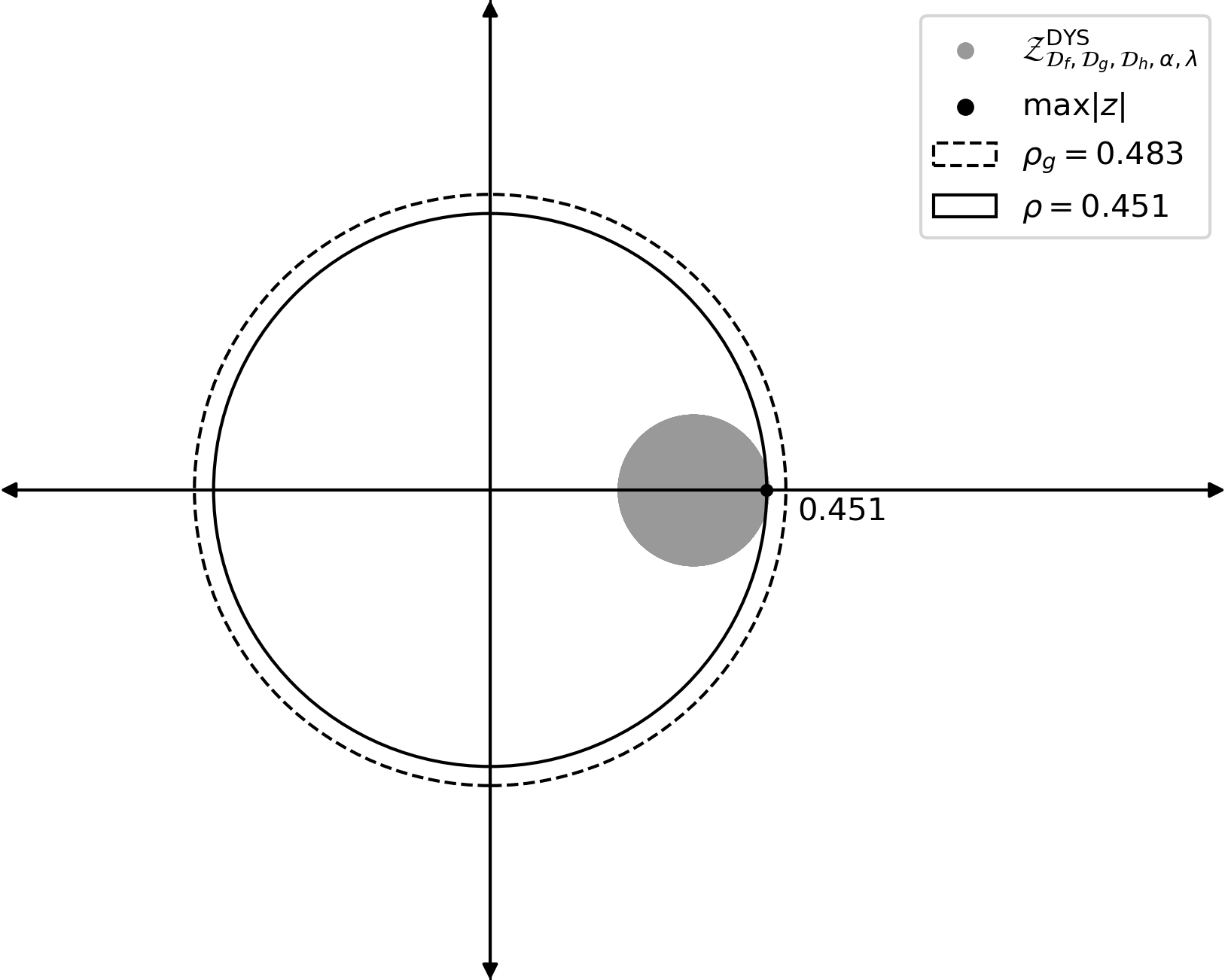
Figure 1: ${\mathcal{Z}}^{\text{DYS}}_{{\mathcal{D}}_{f},{\mathcal{D}}_{g},{\mathcal{D}}_{h},\alpha,\lambda}$ with ${\mathrm{Circ}}(0,\rho_{f})$, ${\mathrm{Circ}}(0,\rho_{g})$, and ${\mathrm{Circ}}(0,\rho)$, where $\mu_{f}=0.7$, $\mu_{g}=2$, $\mu_{h}=0.8$, $L_{f}=1.5$, $L_{g}=3$, $L_{h}=1.3$, $\alpha=0.9$, and $\lambda=1$.

References

• [1] D. Davis, W. Yin, A three-operator splitting scheme and its optimization applications, Set-valued and variational analysis 25 (4) (2017) 829–858.
• [2] M. Yan, A new primal–dual algorithm for minimizing the sum of three functions with a linear operator, Journal of Scientific Computing 76 (3) (2018) 1698–1717.
• [3] Y. Wang, H. Zhou, S. Zu, W. Mao, Y. Chen, Three-operator proximal splitting scheme for 3-d seismic data reconstruction, IEEE Geoscience and Remote Sensing Letters 14 (10) (2017) 1830–1834.
• [4] J. A. Carrillo, K. Craig, L. Wang, C. Wei, Primal dual methods for wasserstein gradient flows, Foundations of Computational Mathematics 22 (2) (2022) 389–443.
• [5] D. Van Hieu, L. Van Vy, P. K. Quy, Three-operator splitting algorithm for a class of variational inclusion problems, Bulletin of the Iranian Mathematical Society 46 (4) (2020) 1055–1071.
• [6] M. Weylandt, Splitting methods for convex bi-clustering and co-clustering, 2019 IEEE Data Science Workshop (2019) 237–242.
• [7] H. Heaton, D. McKenzie, Q. Li, S. W. Fung, S. Osher, W. Yin, Learn to predict equilibria via fixed point networks, arXiv preprint arXiv:2106.00906 (2021).
• [8] F. J. Aragón-Artacho, D. Torregrosa-Belén, A direct proof of convergence of Davis–Yin splitting algorithm allowing larger stepsizes, Set-Valued and Variational Analysis 30 (2022) 1–19.
• [9] M. N. Dao, H. M. Phan, An adaptive splitting algorithm for the sum of three operators, arXiv:2104.05460 (2021).
• [10] F. Pedregosa, On the convergence rate of the three operator splitting scheme, arXiv preprint arXiv:1610.07830 (2016).
• [11] E. K. Ryu, A. B. Taylor, C. Bergeling, P. Giselsson, Operator splitting performance estimation: Tight contraction factors and optimal parameter selection, SIAM Journal on Optimization 30 (3) (2020) 2251–2271.
• [12] H. Wang, M. Fazlyab, S. Chen, V. M. Preciado, Robust convergence analysis of three-operator splitting, Allerton Conference on Communication, Control, and Computing (2019).
• [13] L. Condat, P. Richtárik, RandProx: Primal-Dual Optimization Algorithms with Randomized Proximal Updates (2022). arXiv:2207.12891.
• [14] J. Lee, S. Yi, E. K. Ryu, Convergence Analyses of Davis-Yin Splitting via Scaled Relative Graphs, arXiv preprint arXiv:2207.04015 (2022). arXiv:2207.04015.
• [15] E. K. Ryu, R. Hannah, W. Yin, Scaled relative graphs: Nonexpansive operators via 2D Euclidean geometry, Mathematical Programming 194 (1–2) (2022) 569–619.
• [16] H. H. Bauschke, P. L. Combettes, Convex Analysis and Monotone Operator Theory in Hilbert Spaces, 2nd Edition, Springer, 2017.
• [17] E. K. Ryu, S. Boyd, Primer on monotone operator methods, Appl. Comput. Math 15 (1) (2016) 3–43.
• [18] E. K. Ryu, W. Yin, Large-scale convex optimization via monotone operators, Cambridge University Press, 2022.
• [19] R. E. Bruck, On the weak convergence of an ergodic iteration for the solution of variational inequalities for monotone operators in Hilbert space, Journal of Mathematical Analysis and Applications 61 (1) (1977) 159–164.
• [20] G. B. Passty, Ergodic convergence to a zero of the sum of monotone operators in Hilbert space, Journal of Mathematical Analysis and Applications 72 (2) (1979) 383–390.
• [21] D. W. Peaceman, H. H. Rachford, Jr, The numerical solution of parabolic and elliptic differential equations, Journal of the Society for Industrial and Applied Mathematics 3 (1) (1955) 28–41.
• [22] J. Douglas, H. H. Rachford, On the numerical solution of heat conduction problems in two and three space variables, Transactions of the American Mathematical Society 82 (2) (1956) 421–439.
• [23] P.-L. Lions, B. Mercier, Splitting algorithms for the sum of two nonlinear operators, SIAM Journal on Numerical Analysis 16 (6) (1979) 964–979.
• [24] D. Gabay, B. Mercier, A dual algorithm for the solution of nonlinear variational problems via finite element approximation, Computers & Mathematics with Applications 2 (1) (1976) 17–40.
• [25] A. Yurtsever, A. Gu, S. Sra, Three operator splitting with subgradients, stochastic gradients, and adaptive learning rates, NeurIPS (2021).
• [26] A. Yurtsever, B. C. Vũ, V. Cevher, Stochastic three-composite convex minimization, NeurIPS (2016).
• [27] V. Cevher, B. C. Vũ, A. Yurtsever, Stochastic forward Douglas–Rachford splitting method for monotone inclusions, in: A. R. Pontus Giselsson (Ed.), Large-Scale and Distributed Optimization, Springer, 2018, pp. 149–179.
• [28] A. Yurtsever, V. Mangalick, S. Sra, Three Operator Splitting with a Nonconvex Loss Function, ICML (2021).
• [29] F. Pedregosa, K. Fatras, M. Casotto, Proximal splitting meets variance reduction, in: AISTATS, 2019.
• [30] C. Zong, Y. Tang, Y. J. Cho, Convergence analysis of an inexact three-operator splitting algorithm, Symmetry 10 (11) (2018) 563.
• [31] F. Pedregosa, G. Gidel, Adaptive three operator splitting, ICML (2018).
• [32] F. Cui, Y. Tang, Y. Yang, An inertial three-operator splitting algorithm with applications to image inpainting, Applied Set-Valued Analysis and Optimization 1 (2019).
• [33] A. Salim, L. Condat, K. Mishchenko, P. Richtárik, Dualize, split, randomize: Toward fast nonsmooth optimization algorithms, Journal of Optimization Theory and Applications (2022).
• [34] X. Huang, E. K. Ryu, W. Yin, Scaled relative graph of normal matrices, arXiv preprint arXiv:2001.02061 (2019).
• [35] R. Pates, The Scaled Relative Graph of a Linear Operator, arXiv preprint arXiv:2106.05650 (2021).
• [36] N. Ogura, I. Yamada, Non-strictly convex minimization over the fixed point set of an asymptotically shrinking nonexpansive mapping, Numerical Functional Analysis and Optimization 23 (1-2) (2002) 113–137.
• [37] X. Huang, E. K. Ryu, W. Yin, Tight coefficients of averaged operators via scaled relative graph, Journal of Mathematical Analysis and Applications 490 (1) (2020) 124211.
• [38] T. Chaffey, F. Forni, R. Sepulchre, Graphical Nonlinear System Analysis, arXiv preprint arXiv:2107.11272 (2021).
• [39] T. Chaffey, F. Forni, R. Sepulchre, Scaled relative graphs for system analysis, IEEE Conference on Decision and Control (2021).
• [40] T. Chaffey, R. Sepulchre, Monotone one-port circuits, arXiv preprint arXiv:2111.15407 (2021).
• [41] T. Chaffey, A rolled-off passivity theorem, Systems & Control Letters 162 (2022) 105198.
• [42] T. Chaffey, A. Padoan, Circuit model reduction with scaled relative graphs, arXiv preprint arXiv:2204.01434 (2022).
• [43] Y. Nesterov, Introductory Lectures on Convex Optimization: A Basic Course (2014).