Double Data Piling for Heterogeneous Covariance Models

Abstract

In this work, we characterize two data piling phenomenon for a high-dimensional binary classification problem with heterogeneous covariance models. The data piling refers to the phenomenon where projections of the training data onto a direction vector have exactly two distinct values, one for each class. This first data piling phenomenon occurs for any data when the dimension $p$ is larger than the sample size $n$. We show that the second data piling phenomenon, which refers to a data piling of independent test data, can occur in an asymptotic context where $p$ grows while $n$ is fixed. We further show that a second maximal data piling direction, which gives an asymptotic maximal distance between the two piles of independent test data, can be obtained by projecting the first maximal data piling direction onto the nullspace of the common leading eigenspace. This observation provides a theoretical explanation for the phenomenon where the optimal ridge parameter can be negative in the context of high-dimensional linear classification. Based on the second data piling phenomenon, we propose various linear classification rules which ensure perfect classification of high-dimension low-sample-size data under generalized heterogeneous spiked covariance models.

Keywords: High dimension low sample size, Classification, Maximal data piling, Spiked covariance model, High-dimensional asymptotics

1 Introduction

High-Dimension Low-Sample-Size (HDLSS) data have often been found in many of scientific fields, such as microarray gene expression analysis, chemometrics, and image processing. Such HDLSS data are oftentimes best classified by linear classifiers since the dimension of data $p$ is much larger than the sample size $n$. For binary classification with $p>n$, Ahn and Marron (2010) observed the data piling phenomenon, that is, projections of the training data onto a direction vector $w$ are identical for each class. Among such directions exhibiting data piling, the maximal data piling direction uniquely gives the largest distance between the two piles of training data. The maximal data piling direction is defined as

$w_{\textup{MDP}}=\mathop{\rm argmax}\limits_{w:\|w\|=1}{\left(w^{\top}\mathbf{S}_{B}w\right)}$ subject to $w^{\top}\mathbf{S}_{W}w=0$,

where $\mathbf{S}_{W}$ is the $p\times p$ within-class scatter matrix and $\mathbf{S}_{B}$ is the $p\times p$ between-class scatter matrix of training dataset $\mathcal{X}$. Ahn and Marron (2010) observed that a classification rule using $w_{\textup{MDP}}$ as the normal vector to a discriminative hyperplane achieves better classification performance than classical linear classifiers when there are significantly correlated variables.

However, the maximal data piling direction has not been considered as an appropriate classifier since it depends too much on training data, resulting in poor generalization performances (Marron et al., 2007; Lee et al., 2013). In general, while the training data are piled on $w_{\textup{MDP}}$, independent test data are not piled on $w_{\textup{MDP}}$. Recently, Chang et al. (2021) revealed the existence of the second data piling direction, which gives a data piling of independent test data, under the HDLSS asymptotic regime of Hall et al. (2005) where the dimension of data $p$ tends to grow while the sample size $n$ is fixed. In addition, they showed that a negatively ridged linear discriminant vector, projected onto a low-dimensional subspace, can be a second maximal data piling direction, which yields a maximal asymptotic distance between two piles of independent test data.

A second data piling direction is defined asymptotically as $p\to\infty$, unlike the first data piling of training dataset $\mathcal{X}$ for any fixed $p>n$. For a sequence of directions $\left\{w\right\}=(w^{(1)},\ldots,w^{(p-1)},w^{(p)},w^{(p+1)},\ldots)$, in which $w^{(q)}\in\mathbb{R}^{q}$ for $q\in\mathbb{N}$, we write $w\in\mathbb{R}^{p}$ for the $p$th element of $\left\{w\right\}$. Let $Y,Y^{\prime}$ be independent random vectors from the same population of $\mathcal{X}$, and write $\pi(Y)=k$ if $Y$ belongs to class $k$. Chang et al. (2021) defined the collection of all sequences of second data piling directions as

$$\mathcal{A}=\left\{\left\{w\right\}\in\mathfrak{W}_{X}:\text{ for any }Y,Y^{\prime}\text{ with }\pi(Y)=\pi(Y^{\prime}),~{}p^{-1/2}w^{\top}(Y-Y^{\prime})\xrightarrow{P}0\text{ as }p\to\infty\right\}$$

where $\mathfrak{W}_{X}=\left\{\left\{w\right\}:w\in\mathcal{S}_{X},\|w\|=1\text{ for all }p\right\}$, and $\mathcal{S}_{X}={\rm span}(\mathbf{S}_{W})\cup{\rm span}(\mathbf{S}_{B})$ is the sample space. Furthermore, among the sequences of second data piling directions in $\mathcal{A}$, if $\left\{v\right\}\in\mathcal{A}$ satisfies

$\left\{v\right\}\in\mathop{\rm argmax}\limits_{\left\{w\right\}\in\mathcal{A}}{D(w)}$,

where $D(w)$ is the probability limit of $p^{-1/2}|w^{\top}(Y_{1}-Y_{2})|$ for $\pi(Y_{k})=k$ $(k=1,2)$, then we call $v$ a second maximal data piling direction. Note that a second maximal data piling direction does not uniquely exist as opposed to $w_{\textup{MDP}}$: For $\left\{v_{1}\right\}\in\mathcal{A}$ satisfying $D(w)\leq D(v_{1})$ for any $\left\{w\right\}\in\mathcal{A}$, if $\|v_{1}-v_{2}\|\xrightarrow{P}0$ as $p\to\infty$ for some $\left\{v_{2}\right\}\in\mathcal{A}$, then $\left\{v_{2}\right\}$ also satisfies $D(w)\leq D(v_{2})$ for any $\left\{w\right\}\in\mathcal{A}$.

Chang et al. (2021) showed that the second maximal data piling direction exists and by using such a direction, asymptotic perfect classification of independent test data is possible. They assumed that the population mean difference is as large as $\|\mbox{\boldmath{$\mu$}}_{(1)}-\mbox{\boldmath{$\mu$}}_{(2)}\|=O(p^{1/2})$ and each of two populations has a homogeneous spiked covariance matrix. The spiked covariance model, first introduced by Johnstone (2001), refers to high-dimensional population covariance matrix structures in which a few eigenvalues of the matrix are much larger than the other nearly constant eigenvalues (Ahn et al., 2007; Jung and Marron, 2009; Shen et al., 2016). More precisely, Chang et al. (2021) assumed the common covariance matrix $\Sigma$ has $m$ spikes, that is, $m$ eigenvalues increase at the order of $p^{\beta}$ as $p\to\infty$ with some $\beta\in[0,1]$, while the other eigenvalues are nearly constant, averaging to $\tau^{2}>0$.

With such assumptions, Chang et al. (2021) showed that if $\Sigma$ has weak spikes (that is, $0\leq\beta<1$), then projections of independent test data are asymptotically piled on two distinct points on $w_{\textup{MDP}}$ as $p\to\infty$, similar to the projections of the training data. However, if $\Sigma$ has strong spikes (that is, $\beta=1$), then projections of independent test data tend to be respectively distributed along two parallel affine subspaces in a low-dimensional subspace $\mathcal{S}={\rm span}(\hat{\mathbf{u}}_{1},\ldots,\hat{\mathbf{u}}_{m},w_{\textup{MDP}})\subset\mathcal{S}_{X}$, where $\hat{\mathbf{u}}_{i}$ is the $i$th eigenvector of $\mathbf{S}_{W}$. See Figure 1 for an illustration. Furthermore, they showed that $v_{\alpha}$, which is obtained by projecting a ridged linear discrimination vector onto $\mathcal{S}$, is asymptotically orthogonal to these affine subspaces when the negative ridge parameter $\alpha:=-\tau^{2}$ is used. Figure 1 displays that the projections of independent test data onto $v_{-\tau^{2}}$ are asymptotically piled on two distinct points, one for each class.

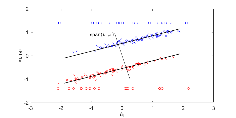
Figure 1: Double data piling phenomenon for homogeneous covariance model with one strong spike ($m=1$). The projections of training dataset are piled on two distinct points on $w_{\textup{MDP}}$. The projections of independent test dataset are distributed along parallel lines in $\mathcal{S}={\rm span}(\hat{\mathbf{u}}_{1},w_{\textup{MDP}})$, which appear to be orthogonal to $v_{-\tau^{2}}$.

In this work, we show that, under generalized heterogeneous spiked covariance models, the second data piling phenomenon occurs when the dimension of data $p$ grows while the sample size $n$ is fixed, and a second maximal data piling direction can be also obtained purely from the training data. We assume that for $k=1,2$, the $k$th class has the covariance matrix $\mbox{\boldmath{$\Sigma$}}_{(k)}$, which has $m_{k}$ spikes such that $m_{k}$ eigenvalues increase at the order of $p^{\beta_{k}}$ as $p\to\infty$ while the other eigenvalues are nearly constant, averaging to $\tau_{k}^{2}>0$. We say that $\mbox{\boldmath{$\Sigma$}}_{(k)}$ has strong spikes if $\beta_{k}=1$, or weak spikes if $0\leq\beta_{k}<1$. Also, we say that two covariance matrices have equal tail eigenvalues if $\tau_{1}^{2}=\tau_{2}^{2}$, or unequal tail eigenvalues if $\tau_{1}^{2}\neq\tau_{2}^{2}$.

Main Contributions

We provide a complete characterization of the second data piling phenomenon under generalized heterogeneous spiked covariance models, which includes a wide range of scenarios where both covariance matrices have either strong spikes ($\beta_{k}=1$) or weak spikes ($\beta_{k}<1$), and have either equal tail eigenvalues ($\tau_{1}^{2}=\tau_{2}^{2}$) or unequal tail eigenvalues ($\tau_{1}^{2}\neq\tau_{2}^{2}$). We show that projections of independent test data tend to be respectively distributed along two affine subspaces, denoted $L_{1}$ and $L_{2}$, in a low-dimensional subspace $\mathcal{S}\subset\mathcal{S}_{X}$. The ‘signal’ subspace $\mathcal{S}$, spanned by some sample eigenvectors of $\mathbf{S}_{W}$ and $w_{\textup{MDP}}$, is obtained by removing the noisy directions from $\mathcal{S}_{X}$, and is also characterized for each of the scenarios. Both affine subspaces $L_{1}$ and $L_{2}$ may not be parallel to each other under heterogeneous covariance assumptions, but we show that there are two parallel affine subspaces of greater dimension, containing each of these affine subspaces, in $\mathcal{S}$. Also, under heterogeneous covariance assumptions, we find a counter-intuitive phenomenon that the eigenvectors of $\mathbf{S}_{W}$ corresponding to the largest eigenvalues do not always contribute to $\mathcal{S}$, but some other seemingly unimportant eigenvectors capture important variability of independent test data. Nonetheless, we show that second data piling occurs for any direction which is asymptotically perpendicular to the parallel affine subspaces. Moreover, we provide a unified view on the second maximal data piling direction for heterogeneous covariance models: The second maximal data piling direction can be obtained by projecting $w_{\textup{MDP}}$ onto the nullspace of the common leading eigenspace.

Based on the characterization of the second data piling phenomenon, we propose various linear classification rules that achieve perfect classification under heterogeneous covariance models. Firstly, for the case of weak spikes ($\beta_{1},\beta_{2}<1$), we show that $w_{\textup{MDP}}$, which is a ridgeless estimator in the context of linear classification setting, also interpolates independent test data. We further show that a bias-corrected maximal data piling classification rule, which is a bias-corrected version of the original maximal data piling classification rule of Ahn and Marron (2010), achieves asymptotic perfect classification for this case. However, for the case of strong spikes ($\beta_{1}=\beta_{2}=1$), linear classification rules based on $w_{\textup{MDP}}$ do not provide the asymptotic perfect classification. For the case where $\beta_{1}\leq 1$ and $\beta_{2}\leq 1$ but with equal tail eigenvalues $(\tau_{1}^{2}=\tau_{2}^{2})$, we show that the negatively ridged linear discriminant vector, projected onto $\mathcal{S}$, can be a second maximal data piling direction even under heterogeneous covariance models. We further show that this direction can be obtained purely from training data, and the original projected ridge classification rule of Chang et al. (2021) achieves perfect classification in more general settings. However, for the case of strong spikes and unequal tail eigenvalues ($\beta_{1}=\beta_{2}=1$ and $\tau_{1}^{2}\neq\tau_{2}^{2}$), the projected ridged linear discriminant vector may not be a second maximal data piling direction, or may not even yield second data piling for any ridge parameter. For all cases mentioned above, we propose Second Maximal Data Piling (SMDP) algorithms, which estimate a second maximal data piling direction by projecting $w_{\textup{MDP}}$ onto the nullspace of the common leading eigenspace, based on a data-splitting approach, and compute discrimination rules based on the estimated directions. The resulting classifiers achieve asymptotic perfect classification for generalized heterogeneous spiked covariance models.

Our main contributions are summarized in the following:

• A complete characterization of the second data piling phenomenon.

  • We categorize the second data piling phenomenon by the magnitude of spikes with equal or unequal tail eigenvalues; see Section 3 and Appendix B.

  • We provide a unified view on the second maximal data piling direction for heterogeneous covariance models: The second maximal data piling direction can be obtained by projecting $w_{\textup{MDP}}$ onto the nullspace of the common leading eigenspace; see Section 5.3.

• Perfect classification based on the second data piling phenomenon.

  • We show that the second data piling direction asymptotically interpolates independent test data, and thus can yield perfect classification.

  • We reveal exact conditions for which the projected ridged linear discriminant vector with a negative ridge parameter yields perfect classification, under the HDLSS asymptotics; see Section 4, Sections 5.1–5.2 and Appendices A and B.

  • We develop Second Maximal Data Piling (SMDP) algorithms which ensure perfect classification for generalized heterogeneous spiked covariance models; see Sections 5.4–5.5.

Related Works

There has been relatively scarce works on a binary classification problem for cases where $\mbox{\boldmath{$\Sigma$}}_{(1)}$ or $\mbox{\boldmath{$\Sigma$}}_{(2)}$ has strong spikes, which reflects much more realistic and interesting situations for HDLSS data. Aoshima and Yata (2019) proposed a distance-based classifier, while Ishii et al. (2022) proposed geometrical quadratic discriminant analysis for this problem. Both assume not only the dimension of data $p$ but also training sample sizes of each class $n_{1}$ and $n_{2}$ tend to infinity to achieve perfect classification. Ishii (2020) proposed another distance-based classifier which achieves perfect classification even when $n_{1}$ and $n_{2}$ are fixed, but limited to the one-component covariance model (with $m_{1}=m_{2}=1$). All of these works are based on a data transformation technique, which essentially projecting the independent test data onto the nullspace of the leading eigenspace. Our results are also based on a similar idea of removing the leading eigenspace, but we further suggest the concept of double data piling phenomenon and reveal the relationship between the maximal data piling direction of training data and the second maximal data piling direction of independent test data under generalized heterogeneous spiked covariance models.

It has been frequently observed that extremely complicated models which interpolate training data can also achieve nearly zero generalization error, which contradicts an important concept of the classical statistical learning framework in which a careful regularization is inevitable to achieve small generalization error (Zhang et al., 2017; Belkin et al., 2019). Recently, this phenomenon has been confirmed both empirically and theoretically in the context of linear regression (Bartlett et al., 2020; Holzmüller, 2020; Hastie et al., 2022), and it turned out that a (nearly) zero ridge parameter can be optimal in the overparameterized regime of $p>n$ (called benign overfitting). Kobak et al. (2020) showed that the optimal ridge parameter can be negative using one-component covariance model in the overparameterized regime, and Tsigler and Bartlett (2020) further showed that negative regularization can achieve small generalization error than nearly zero regularization under specific spiked covariance models. Wu and Xu (2020) also provided general conditions when the optimal ridge parameter is negative in the overparameterized regime. Our findings are consistent with the above results concerning linear regression, and provide conditions when negative regularization is needed in the context of linear classification. Note that $w_{\textup{MDP}}$, which is a ridgeless estimator in the classification setting, successfully interpolates independent test data when the variables are weakly correlated. The projected ridged linear discriminant vector with a negative ridge parameter interpolates independent test data when the variables are strongly correlated and both classes have equal tail eigenvalues. In the linear classification setting, the generalization error of maximum margin classifiers is also examined in the overparameterized regime (Montanari et al., 2019; Chatterji and Long, 2021).

Organization

The rest of this paper is organized as follows. In Section 2, we specifically define the generalized heterogeneous spiked covariance models. In Section 3, we characterize the second data piling phenomenon under the heterogeneous covariance models for $\beta_{1},\beta_{2}<1$ or $\beta_{1}=\beta_{2}=1$ (Discussions for $\beta_{1}=1,\beta_{2}<1$ or $\beta_{1}<1,\beta_{2}=1$ are given in Appendix B). In Section 4, we study the case for which the projected ridged linear discriminant vector with a negative ridge parameter is a second maximal data piling direction. In Section 5, we show that a second maximal data piling direction can be obtained by projecting $w_{\textup{MDP}}$ onto the common leading eigenspace. By noting this fact, we propose Second Maximal Data Piling (SMDP) algorithms to estimate a second maximal data piling direction. In Section 6, we numerically confirm performances of classification rules based on the projected ridged linear discriminant vector and SMDP algorithms. The bias-corrected projected ridge classification rule is given in Appendix A. We provide asymptotic properties of high-dimensional sample within-scatter matrix $\mathbf{S}_{W}$ in Appendix C. The proofs of main lemmas and theorems are contained in Appendix D.

2 Heterogeneous Covariance Models

We assume that for $k=1,2$, $X|\pi(X)=k$ follows an absolutely continuous distribution on $\mathbb{R}^{p}$ with mean $\mbox{\boldmath{$\mu$}}_{(k)}$ and covariance matrix $\mbox{\boldmath{$\Sigma$}}_{(k)}$. Also, we assume $\mathbb{P}(\pi(X)=k)=\pi_{k},$ where $\pi_{k}>0$ and $\pi_{1}+\pi_{2}=1$. Write the eigen-decomposition of $\mbox{\boldmath{$\Sigma$}}_{(k)}$ by $\mbox{\boldmath{$\Sigma$}}_{(k)}=\mathbf{U}_{(k)}\mbox{\boldmath{$\Lambda$}}_{(k)}\mathbf{U}_{(k)}^{\top}$, where $\mbox{\boldmath{$\Lambda$}}_{(k)}=\mbox{Diag}{(\lambda_{(k),1},\ldots,\lambda_{(k),p})}$ in which the eigenvalues are arranged in descending order, and $\mathbf{U}_{(k)}=[\mathbf{u}_{(k),1},\ldots,\mathbf{u}_{(k),p}]$ for $k=1,2$. Let the horizontally concatenated data matrix

$$\mathbf{X}=[X_{11},\ldots,X_{1n_{1}},X_{21},\ldots,X_{2n_{2}}]$$

be the $p\times n$ data matrix consisting of the $n:=n_{1}+n_{2}$ observations arranged so that $\pi(X_{kj})=k$ for any $k,j$. We assume $n_{1}$ and $n_{2}$ are fixed and denote $\eta_{k}=n_{k}/n$ for $k=1,2$. We write class-wise sample mean vectors $\bar{X}_{k}={n_{k}}^{-1}\sum_{j=1}^{n_{k}}X_{kj}$, and total sample mean vector $\bar{X}=\eta_{1}\bar{X}_{1}+\eta_{2}\bar{X}_{2}$. Also, we write

$$\mathbf{S}_{k}=(\mathbf{X}_{k}-\bar{\mathbf{X}}_{k})(\mathbf{X}_{k}-\bar{\mathbf{X}}_{k})^{\top}$$

for $k=1,2$ and the within-class scatter matrix

$$\mathbf{S}_{W}=\mathbf{S}_{1}+\mathbf{S}_{2}=(\mathbf{X}-\bar{\mathbf{X}})(\mathbf{X}-\bar{\mathbf{X}})^{\top},$$

where $\bar{\mathbf{X}}_{k}=\bar{X}_{k}\mathbf{1}_{n_{k}}^{\top}$ for $k=1,2$ and $\bar{\mathbf{X}}=[\bar{\mathbf{X}}_{1}~{}\bar{\mathbf{X}}_{2}]$. We write an eigen-decomposition of $\mathbf{S}_{W}$ by $\mathbf{S}_{W}=\hat{\mathbf{U}}\hat{}\mbox{\boldmath{$\Lambda$}}\hat{\mathbf{U}}^{\top}$, where $\hat{}\mbox{\boldmath{$\Lambda$}}=\mbox{Diag}{(\hat{\lambda}_{1},\ldots,\hat{\lambda}_{p})}$ in which the eigenvalues are arranged in descending order, and $\hat{\mathbf{U}}=[\hat{\mathbf{u}}_{1},\ldots,\hat{\mathbf{u}}_{p}]$. Since $\hat{\lambda}_{1}\geq\ldots\geq\hat{\lambda}_{n-2}\geq\hat{\lambda}_{n-1}=\ldots=\hat{\lambda}_{p}=0$ with probability $1$, we can write $\mathbf{S}_{W}=\hat{\mathbf{U}}_{1}\hat{}\mbox{\boldmath{$\Lambda$}}_{1}\hat{\mathbf{U}}_{1}^{\top}$ where $\hat{\mathbf{U}}_{1}=[\hat{\mathbf{u}}_{1},\ldots,\hat{\mathbf{u}}_{n-2}]$ and $\hat{}\mbox{\boldmath{$\Lambda$}}_{1}=\mbox{Diag}{(\hat{\lambda}_{1},\ldots,\hat{\lambda}_{n-2})}$. Also, we write $\hat{\mathbf{U}}_{2}=[\hat{\mathbf{u}}_{n-1},\ldots,\hat{\mathbf{u}}_{p}]$. We denote the sample space as $\mathcal{S}_{X}$, which is the $(n-1)$-dimensional subspace spanned by $X_{kj}-\bar{X}$ for $k=1,2$ and $1\leq j\leq n_{k}$. Note that the sample space $\mathcal{S}_{X}$ can be equivalently expressed as ${\rm span}(\hat{\mathbf{u}}_{1},\ldots,\hat{\mathbf{u}}_{n-2},w_{\textup{MDP}})$ (Ahn and Marron, 2010; Chang et al., 2021). We denote the sample mean difference vector as $\mathbf{d}=\bar{\mathbf{X}}_{1}-\bar{\mathbf{X}}_{2}$. Note that the sphered data matrix of $\mathbf{X}_{k}$ is

$$\mathbf{Z}_{(k)}=\mbox{\boldmath{$\Lambda$}}_{(k)}^{-\frac{1}{2}}\mathbf{U}_{(k)}^{\top}(\mathbf{X}_{k}-\mbox{\boldmath{$\mu$}}_{(k)}\mathbf{1}_{n_{k}}^{\top})=\begin{pmatrix}z_{(k),1}^{\top}\\ \vdots\\ z_{(k),p}^{\top}\end{pmatrix}\in\mathbb{R}^{p\times n_{k}}$$

for $k=1,2$. Then the elements of $\mathbf{Z}_{(k)}$ are uncorrelated with each other, and have mean zero and unit variance. We make the following assumptions for generalized heterogeneous spiked covariance models.

Assumption 1

For the population mean difference vector $\mbox{\boldmath{$\mu$}}=\mbox{\boldmath{$\mu$}}_{(1)}-\mbox{\boldmath{$\mu$}}_{(2)}$, there exists $\delta>0$ such that $p^{-1/2}\|\mbox{\boldmath{$\mu$}}\|\to\delta$ as $p\to\infty$.

Assumption 2

For a fixed integer $m_{k}\geq 1$, $\sigma_{(k),i}^{2},\tau_{(k),i}^{2}>0$ and $\beta_{k}\in[0,1]$ $(k=1,2)$, assume that $\lambda_{(k),i}=\sigma_{(k),i}^{2}p^{\beta_{k}}+\tau_{(k),i}^{2}$ for $1\leq i\leq m_{k}$ and $\lambda_{(k),i}=\tau_{(k),i}^{2}$ for $m_{k}+1\leq i\leq p$. Also, $\left\{\tau_{(k),i}^{2}:k=1,2,~{}i=1,2,\ldots\right\}$ is uniformly bounded and $p^{-1}\sum_{i=1}^{p}\tau_{(k),i}^{2}\rightarrow\tau_{k}^{2}$ as $p\to\infty$ for some $\tau_{k}^{2}>0$.

Assumption 1 ensures that nearly all variables are meaningfully contributing to discrimination (Hall et al., 2005; Qiao et al., 2010; Jung, 2018). Assumption 2 allows heterogeneous covariance matrices for different classes, including the homogeneous case, that is, $\mbox{\boldmath{$\Sigma$}}_{(1)}=\mbox{\boldmath{$\Sigma$}}_{(2)}$. We assume for $k=1,2$, $\mbox{\boldmath{$\Sigma$}}_{(k)}$ has $m_{k}$ spikes, that is, $m_{k}$ eigenvalues increase at the order of $p^{\beta_{k}}$ as $p\to\infty$ while the other eigenvalues are nearly constant as $\tau_{k}^{2}$. We call the first $m_{k}$ eigenvalues and their corresponding eigenvectors leading eigenvalues and eigenvectors of the $k$th class for $k=1,2$. We say that $\mbox{\boldmath{$\Sigma$}}_{(k)}$ has strong spikes if $\beta_{k}=1$, or weak spikes if $0\leq\beta_{k}<1$. Also, we say that two covariance matrices have equal tail eigenvalues if $\tau_{1}^{2}=\tau_{2}^{2}$, or unequal tail eigenvalues if $\tau_{1}^{2}\neq\tau_{2}^{2}$. Note that if $\beta_{k}>1$, then $\mbox{\boldmath{$\Sigma$}}_{(k)}$ has extremely strong signals within the leading eigenspace, and thus the classification problem becomes straightforward (Jung and Marron, 2009). Hence, we pay an attention to the cases of $\beta_{1},\beta_{2}\in[0,1]$. Assumption 2 may be relaxed so that the first $m_{k}$ eigenvalues have different orders of magnitude, for example, for some $N_{k}>0$, we may assume $\lambda_{(k),i}=\sigma_{(k),i}^{2}p^{\beta_{k,i}}+\tau_{(k),i}^{2}$ for $1\geq\beta_{k,1}\geq\ldots\geq\beta_{k,N_{k}}\geq 0$. However, asymptotic results under this relaxed model are equivalent with the results under Assumption 2 with some $m_{k}$ under the HDLSS asymptotic regime (see Chang et al., 2021, Remark 2.1).

Also, we regulate the dependency of the principal components by introducing the concept of $\rho$-mixing condition (Kolmogorov and Rozanov, 1960; Bradley, 2005). For any $\sigma$-field $\mathcal{E}$, denote the class of square-integrable and $\mathcal{E}$-measurable random variables as $L_{2}(\mathcal{E})$. Suppose $\left\{Z_{i}:-\infty\leq i\leq\infty\right\}$ is a sequence of random variables. For $-\infty\leq J\leq L\leq\infty$, denote $\mathcal{F}_{J}^{L}$ as the $\sigma$-field of events generated by the random variables $\left\{Z_{i}:J\leq i\leq K\right\}$. Then, for the $\rho$-mixing coefficient

$$\rho(k):=\sup\limits_{j\in\mathbb{Z}}\rho(\mathcal{F}_{-\infty}^{j},\mathcal{F}_{j+n}^{\infty})=\sup\limits_{j\in\mathbb{Z}}\sup\left\{\left|\mbox{Corr}{(f,g)}\right|:f\in\mathcal{L}^{2}(\mathcal{F}_{-\infty}^{j}),g\in\mathcal{L}^{2}(\mathcal{F}_{j+n}^{\infty})\right\},$$

the sequence $\left\{Z_{i}:-\infty\leq i\leq\infty\right\}$ is said to be $\rho$-mixing if $\rho(k)\rightarrow 0$ as $k\to\infty$. We now give a following assumption on the true principal component scores $z_{kj}=\mbox{\boldmath{$\Lambda$}}_{(k)}^{-1/2}\mathbf{U}_{(k)}^{\top}(X_{kj}-\mbox{\boldmath{$\mu$}}_{(k)})\in\mathbb{R}^{p}$ for $k=1,2$ and $1\leq j\leq n_{k}$. This allows us to make use of the law of large numbers applied to $p\to\infty$ introduced in Hall et al. (2005) and Jung and Marron (2009).

Assumption 3

The elements of the $p$-vector $z_{kj}$ have uniformly bounded fourth moments, and for each $p$, $z_{kj}$ consists of the first $p$ elements of an infinite random sequence

$$(z_{(k),1},z_{(k),2},...)_{j},$$

which is $\rho$-mixing under some permutation.

We define ${\rm Angle}(w_{1},w_{2}):=\arccos\left(w_{1}^{\top}w_{2}/\left(\|w_{1}\|_{2}\|w_{2}\|_{2}\right)\right)$ for $w_{1},w_{2}\in\mathbb{R}^{p}\setminus\left\{\mathbf{0}_{p}\right\}$. For $w\in\mathbb{R}^{p}\setminus\left\{\mathbf{0}_{p}\right\}$ and a subspace $\mathcal{V}$ of $\mathbb{R}^{p}$, let $P_{\mathcal{V}}w$ be the orthogonal projection of $w$ onto $\mathcal{V}$ and define ${\rm Angle}(w,\mathcal{V}):=\arccos\left(w^{\top}P_{\mathcal{V}}w/\left(\|w\|_{2}\|P_{\mathcal{V}}w\|_{2}\right)\right)$. Also, for subspaces $\mathcal{H}={\rm span}(h_{1},\ldots,h_{k})$ and $\mathcal{V}$ of $\mathbb{R}^{p}$, we define the projection of $\mathcal{H}$ onto $\mathcal{V}$ as $P_{\mathcal{V}}\mathcal{H}={\rm span}(P_{\mathcal{V}}h_{1},\ldots,P_{\mathcal{V}}h_{k})$. Assumption 4 specifies limiting angles between leading eigenvectors of each class and the population mean difference vector $\mu$. Without loss of generality, we assume $\mathbf{u}_{(k),i}^{\top}\mbox{\boldmath{$\mu$}}\geq 0$ for all $k=1,2$ and $1\leq i\leq m_{k}$.

Assumption 4

For $\theta_{(k),i}\in[0,\pi/2]$, ${\rm Angle}(\mathbf{u}_{(k),i},\mbox{\boldmath{$\mu$}})\to\theta_{(k),i}$ as $p\to\infty$ for $1\leq i\leq m_{k}$ and $k=1,2$.

We write a $p\times m_{k}$ orthonormal matrix of leading eigenvectors of each class as

$$\mathbf{U}_{(k),1}=[\mathbf{u}_{(k),1},\ldots,\mathbf{u}_{(k),m_{k}}]$$

for $k=1,2$. We call $\mathcal{U}_{(k)}={\rm span}(\mathbf{U}_{(k),1})$ the leading eigenspace of the $k$th class. Furthermore, let $\mathcal{U}$ be the subspace spanned by leading eigenvectors whose corresponding eigenvalues increase at the order of $p$, that is,

$$\mathcal{U}=\begin{cases}\mathbf{0}_{p},&\text{if}~{}\beta_{1}<1,\beta_{2}<1,\\ \mathcal{U}_{(1)},&\text{if}~{}\beta_{1}=1,\beta_{2}<1,\\ \mathcal{U}_{(2)},&\text{if}~{}\beta_{1}<1,\beta_{2}=1,\\ {\rm span}(\mathcal{U}_{(1)}\cup\mathcal{U}_{(2)}),&\text{if}~{}\beta_{1}=1,\beta_{2}=1.\end{cases}$$

We call $\mathcal{U}$ the common leading eigenspace of both classes. We assume that the dimension of $\mathcal{U}$,

$$m=\dim{(\mathcal{U})},$$

is a fixed constant for all $p$. Note that

$$m=\begin{cases}0,&\text{if}~{}\beta_{1}<1,\beta_{2}<1,\\ m_{1},&\text{if}~{}\beta_{1}=1,\beta_{2}<1,\\ m_{2},&\text{if}~{}\beta_{1}<1,\beta_{2}=1.\end{cases}$$

Also, note that if $\beta_{1}=1$ and $\beta_{2}=1$, then $\max{(m_{1},m_{2})}\leq m\leq m_{1}+m_{2}$. Write an orthogonal basis of $\mathcal{U}$ as $\mathbf{U}_{1}=[\mathbf{u}_{1},\ldots,\mathbf{u}_{m}]$, satisfying $\mathbf{u}_{i}^{\top}\mbox{\boldmath{$\mu$}}\geq 0$ for all $1\leq i\leq m$. If $\beta_{1}=1$ and $\beta_{2}=1$, then there exist orthogonal matrices $\mathbf{R}_{(k)}^{(p)}\in\mathbb{R}^{m\times m_{k}}$ satisfying $\mathbf{U}_{(k),1}=\mathbf{U}_{1}\mathbf{R}_{(k)}^{(p)}$ for $k=1,2$. Note that the matrix $\mathbf{R}_{(k)}^{(p)}$ catches the angles between the $m_{k}$ leading eigenvectors in $\mathbf{U}_{(k),1}$ and the $m$ basis in $\mathbf{U}_{1}$. We assume the following.

Assumption 5

For $\theta_{i}\in[0,\pi/2]$, there exists a basis $\mathbf{u}_{1},\ldots,\mathbf{u}_{m}$ such that ${\rm Angle}(\mathbf{u}_{i},\mbox{\boldmath{$\mu$}})\to\theta_{i}$ as $p\to\infty$ for $1\leq i\leq m$ and for an orthogonal matrix $\mathbf{R}_{(k)}\in\mathbb{R}^{m\times m_{k}}$, $\mathbf{R}^{(p)}_{(k)}\to\mathbf{R}_{(k)}$ as $p\to\infty$ for $k=1,2$. Moreover, $\mathbf{R}=[\mathbf{R}_{(1)}~{}\mathbf{R}_{(2)}]$ is of rank $m$.

Finally, let $\varphi_{k}$ denote the limiting angle between $\mu$ and $\mathcal{U}_{(k)}$ for $k=1,2$. Also, let $\varphi$ denote the limiting angle between $\mu$ and $\mathcal{U}$. Then we have $\cos^{2}\varphi_{1}=\sum_{i=1}^{m_{1}}\cos^{2}\theta_{(1),i}$, $\cos^{2}\varphi_{2}=\sum_{i=1}^{m_{2}}\cos^{2}\theta_{(2),i}$ and $\cos^{2}\varphi=\sum_{i=1}^{m}\cos^{2}\theta_{i}$. Note that $\cos^{2}\varphi=\cos^{2}\varphi_{1}$ if $\beta_{1}=1,\beta_{2}<1$ and $\cos^{2}\varphi=\cos^{2}\varphi_{2}$ if $\beta_{1}<1,\beta_{2}=1$. Also, we use the convention that if the dimension $m$ of $\mathcal{U}$ is zero $(\beta_{1}<1,\beta_{2}<1)$, then $\varphi=\pi/2$ and $\cos^{2}\varphi=0$.

3 Data Piling of Independent Test Data

In this section, we show that independent test data, projected onto a low-dimensional signal subspace $\mathcal{S}$ of the sample space $\mathcal{S}_{X}$, tend to be respectively distributed along two affine subspaces as $p\to\infty$. Chang et al. (2021) showed that there are two affine subspaces, each with dimension $m=m_{1}=m_{2}$, such that they are parallel to each other if each class has common covariance matrix, that is, $\mbox{\boldmath{$\Sigma$}}_{(1)}=\mbox{\boldmath{$\Sigma$}}_{(2)}$. We show that if $\mbox{\boldmath{$\Sigma$}}_{(1)}\neq\mbox{\boldmath{$\Sigma$}}_{(2)}$, these affine subspaces may not be parallel to each other, but there exist parallel affine subspaces, of greater dimension, containing each of these affine subspaces.

To illustrate this phenomenon, we first consider a simple one-component covariance model for each covariance matrix, that is, $m_{1}=1$ and $m_{2}=1$ in Assumption 2. In Section 3.1, this phenomenon is demonstrated under the one-component covariance model with various conditions on covariance matrices. In Section 3.2, we characterize the signal subspace $\mathcal{S}$, which captures important variability of independent test data, for each scenario of two covariance matrices. In Section 3.3, we provide the main theorem (Theorem 6) that generalizes propositions in Section 3.1 to the cases where $m_{1}\geq 1$ and $m_{2}\geq 1$.

Let $\mathcal{Y}_{k}$ be an independent test data of the $k$th class whose element $Y\in\mathcal{Y}_{k}$ satisfies $\pi(Y)=k$ for $k=1,2$ and is independent to training data $\mathcal{X}$. Write $\mathcal{Y}=\mathcal{Y}_{1}\cup\mathcal{Y}_{2}$.

3.1 One-component Covariance Model

In this subsection, we investigate the data piling phenomenon of independent test data under the one-component covariance model as follows:

$$\mbox{\boldmath{$\Sigma$}}_{(1)}=\sigma_{(1),1}^{2}p\mathbf{u}_{(1),1}\mathbf{u}_{(1),1}^{\top}+\tau_{1}^{2}\mathbf{I}_{p};$$ (1)

$$\mbox{\boldmath{$\Sigma$}}_{(2)}=\sigma_{(2),1}^{2}p\mathbf{u}_{(2),1}\mathbf{u}_{(2),1}^{\top}+\tau_{2}^{2}\mathbf{I}_{p}.$$

Note that this model assumes that both classes have strongly correlated variables, that is, $\beta_{1}=\beta_{2}=1$. We consider various settings where both covariance matrices have either equal tail eigenvalues or unequal tail eigenvalues, and have either a common leading eigenvector or uncommon leading eigenvectors. We provide an overview of our settings in the following.

	$\mathbf{u}_{(1),1}=\mathbf{u}_{(2),1}$	$\mathbf{u}_{(1),1}\neq\mathbf{u}_{(2),1}$
$\tau_{1}^{2}=\tau_{2}^{2}$	Example 1	Example 2
$\tau_{1}^{2}\neq\tau_{2}^{2}$	Example 3	Example 4

We assume the distribution of $X|\pi(X)=k$ for $k=1,2$ is Gaussian in the following examples.

3.1.1 One-component Covariance Model with Equal Tail Eigenvalues

First, we assume that two covariance matrices have equal tail eigenvalues, that is, $\tau_{1}^{2}=\tau_{2}^{2}$. For the sake of simplicity, denote $\tau^{2}:=\tau_{1}^{2}=\tau_{2}^{2}$.

Example 1

We first consider the case where both classes have the common leading eigenvector, that is, $\mathbf{u}_{(1),1}=\mathbf{u}_{(2),1}=\mathbf{u}_{1}$. Note that if $\sigma_{(1),1}^{2}=\sigma_{(2),1}^{2}$, then this model is equivalent to the homogeneous covariance model $\mbox{\boldmath{$\Sigma$}}_{(1)}=\mbox{\boldmath{$\Sigma$}}_{(2)}$, studied in Chang et al. (2021).

It turns out that the angle between $\hat{\mathbf{u}}_{1}$ and $\mathbf{u}_{1}$ converges to a random quantity between $0$ and $\pi/2$, while $\hat{\mathbf{u}}_{2},\ldots,\hat{\mathbf{u}}_{n-2}$ are strongly inconsistent with $\mathbf{u}_{1}$ in the sense that ${\rm Angle}(\hat{\mathbf{u}}_{i},\mathbf{u}_{1})\xrightarrow{P}\pi/2$ as $p\to\infty$ for $2\leq i\leq n-2$. For this case, let $\mathcal{D}=\left\{1\right\}$. We can check that even if $\sigma_{(1),1}^{2}\neq\sigma_{(2),1}^{2}$, projections of independent test data $\mathcal{Y}$ onto $\mathcal{S}={\rm span}(\left\{\hat{\mathbf{u}}_{i}\right\}_{i\in\mathcal{D}},w_{\textup{MDP}})={\rm span}(\hat{\mathbf{u}}_{1},w_{\textup{MDP}})$ tend to be distributed along two parallel lines, while those of training data $\mathcal{X}$ are piled on two distinct points along $w_{\textup{MDP}}$. This result is consistent with the findings of Chang et al. (2021) where $\mbox{\boldmath{$\Sigma$}}_{(1)}=\mbox{\boldmath{$\Sigma$}}_{(2)}$; see Figure 1. Also, the direction of these lines are asymptotically parallel to $P_{\mathcal{S}}\mathbf{u}_{1}$, which is the projection of common leading eigenvector $\mathbf{u}_{1}$ onto $\mathcal{S}$; see Proposition 1.

Example 2

Two classes do not have a common leading eigenvector, that is, $\mathbf{u}_{(1),1}\neq\mathbf{u}_{(2),1}$, such that the angle between $\mathbf{u}_{(1),1}$ and $\mathbf{u}_{(2),1}$ is $\pi/4$. Under this model, the common leading eigenspace has the dimension $m=2$ (In contrast, $m=1$ in the model of Example 1).

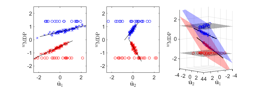
Figure 2: $2$-dimensional projections onto $\mathcal{S}_{1}={\rm span}(\hat{\mathbf{u}}_{1},w_{\textup{MDP}})$ and $\mathcal{S}_{2}={\rm span}(\hat{\mathbf{u}}_{2},w_{\textup{MDP}})$ and $3$-dimensional projections onto $\mathcal{S}={\rm span}(\left\{\hat{\mathbf{u}}_{i}\right\}_{i\in\mathcal{D}},w_{\textup{MDP}})$ with $\mathcal{D}=\left\{1,2\right\}$ of training data $\mathcal{X}$ (class 1: blue circles, class 2: red circles) and independent test data $\mathcal{Y}$ (class 1: blue crosses, class 2: red crosses) under the model in Example 2.

In this case, it turns out that the angle between $\hat{\mathbf{u}}_{i}$ and $\mathcal{U}={\rm span}(\mathbf{u}_{(1),1},\mathbf{u}_{(2),1})$ converges to a random quantity between $0$ and $\pi/2$ for $i=1,2$, while the other sample eigenvectors are strongly inconsistent with $\mathcal{U}$. Let $\mathcal{D}=\left\{1,2\right\}$. In Figure 2, independent test data $\mathcal{Y}$ projected onto $\mathcal{S}_{1}={\rm span}(\hat{\mathbf{u}}_{1},w_{\textup{MDP}})$ and $\mathcal{S}_{2}={\rm span}(\hat{\mathbf{u}}_{2},w_{\textup{MDP}})$ are also concentrated along lines, but in both subspaces these lines are not parallel to each other. However, within the $3$-dimensional subspace $\mathcal{S}={\rm span}(\left\{\hat{\mathbf{u}}_{i}\right\}_{i\in\mathcal{D}},w_{\textup{MDP}})={\rm span}(\hat{\mathbf{u}}_{1},\hat{\mathbf{u}}_{2},w_{\textup{MDP}})$, there are two parallel $2$-dimensional planes including these lines, one for each line. In fact, $\mathcal{Y}_{1}$ is distributed along the direction $P_{\mathcal{S}}\mathbf{u}_{(1),1}$, while $\mathcal{Y}_{2}$ is distributed along the direction $P_{\mathcal{S}}\mathbf{u}_{(2),1}$. Thus, these lines are asymptotically contained in $2$-dimensional affine subspaces, that are parallel to $P_{\mathcal{S}}\mathcal{U}={\rm span}(P_{\mathcal{S}}\mathbf{u}_{(1),1},P_{\mathcal{S}}\mathbf{u}_{(2),1})$.

We formally state the above results. Write the training data piling distance as

$$\kappa_{\textup{MDP}}=p^{-1/2}\|w_{\textup{MDP}}^{\top}(\bar{X}_{1}-\bar{X}_{2})\|.$$ (2)

For $Y\in\mathcal{Y}$ and a subspace $\mathcal{S}$ of $\mathbb{R}^{p}$, let $Y_{\mathcal{S}}=p^{-1/2}P_{\mathcal{S}}Y$, which is a scaled projection of $Y$ onto $\mathcal{S}$. Similarly, write ${\bar{X}}_{\mathcal{S}}=p^{-1/2}P_{\mathcal{S}}\bar{X}$. Recall that $\mathbf{u}_{1},\ldots,\mathbf{u}_{m}$ are orthogonal basis of the common leading eigenspace $\mathcal{U}={\rm span}(\mathbf{u}_{1},\ldots,\mathbf{u}_{m})$. Let projections of $\mathbf{u}_{i}$ onto $\mathcal{S}$ as $\mathbf{u}_{i,\mathcal{S}}=P_{\mathcal{S}}\mathbf{u}_{i}$ and write $\mathbf{U}_{1,\mathcal{S}}=[\mathbf{u}_{1,\mathcal{S}},\ldots,\mathbf{u}_{m,\mathcal{S}}]$. The following proposition states that for $m=1,2$, projections of $\mathcal{Y}$ onto the $(m+1)$-dimensional subspace $\mathcal{S}={\rm span}(\hat{\mathbf{u}}_{1},\ldots,\hat{\mathbf{u}}_{m},w_{\textup{MDP}})$ are distributed along two $m$-dimensional affine subspaces, which become parallel to each other, and also to $P_{\mathcal{S}}\mathcal{U}={\rm span}(\mathbf{u}_{1,\mathcal{S}},\ldots,\mathbf{u}_{m,\mathcal{S}})$, as $p$ increases.

Proposition 1

Suppose Assumptions 1—5 hold and assume $\beta_{1}=\beta_{2}=1$, $\tau_{1}^{2}=\tau_{2}^{2}$ and $m_{1}=m_{2}=1$. Also,

• if $m=1$, let $\mathcal{S}={\rm span}(\hat{\mathbf{u}}_{1},w_{\textup{MDP}})$ and $L_{k}=\left\{\mathbf{u}_{1,{\mathcal{S}}}t+\nu_{k}w_{\textup{MDP}}+\bar{X}_{\mathcal{S}}:t\in\mathbb{R}\right\}$,

• if $m=2$, let $\mathcal{S}={\rm span}(\hat{\mathbf{u}}_{1},\hat{\mathbf{u}}_{2},w_{\textup{MDP}})$ and $L_{k}=\left\{\mathbf{U}_{1,{\mathcal{S}}}\mathbf{t}+\nu_{k}w_{\textup{MDP}}+\bar{X}_{\mathcal{S}}:\mathbf{t}\in\mathbb{R}^{2}\right\}$

for $k=1,2$ where $\nu_{1}=\kappa_{\textup{MDP}}^{-1}\left(\eta_{2}(1-\cos^{2}\varphi)\delta^{2}\right)$ and $\nu_{2}=\kappa_{\textup{MDP}}^{-1}\left(-\eta_{1}(1-\cos^{2}\varphi)\delta^{2}\right)$. Then for any independent observation $Y\in\mathcal{Y}$ and for any $\epsilon>0$,

$$\lim\limits_{p\to\infty}\mathbb{P}\left(\inf\limits_{a\in L_{k}}\|Y_{\mathcal{S}}-a\|>\epsilon|\pi(Y)=k\right)=0$$

for $k=1,2$.

Note that if $m=1$, then $\mathcal{Y}_{k}$ is concentrated along the line $L_{k}$ in $\mathcal{S}={\rm span}(\hat{\mathbf{u}}_{1},w_{\textup{MDP}})$, for $k=1,2$. If $m=2$, then $\mathcal{Y}_{k}$ is concentrated along a line $L_{k}^{\prime}$, which is parallel to $P_{\mathcal{S}}\mathbf{u}_{(k),1}$ in $\mathcal{S}={\rm span}(\hat{\mathbf{u}}_{1},\hat{\mathbf{u}}_{2},w_{\textup{MDP}})$, for $k=1,2$. Then each of the $2$-dimensional subspaces $L_{1}$ and $L_{2}$ contains $L_{1}^{\prime}$ and $L_{2}^{\prime}$ respectively, and these subspaces are parallel to each other.

3.1.2 One-component Covariance Model with Unequal Tail Eigenvalues

We now assume that two covariance matrices have unequal tail eigenvalues, that is, $\tau_{1}^{2}\neq\tau_{2}^{2}$. Without loss of generality, we assume $\tau_{1}^{2}>\tau_{2}^{2}$. In this case, asymptotic properties of sample eigenvectors of $\mathbf{S}_{W}$ are quite different from the case where $\tau_{1}^{2}=\tau_{2}^{2}$. See Remark 1.

Remark 1

Let $Y=\tau_{1}Y_{1}U+\tau_{2}Y_{2}(1-U)=(y_{1},\ldots,y_{p})^{\top}\in\mathbb{R}^{p}$, where $Y_{1},Y_{2}$ are two independent $\mathcal{N}_{p}(\mathbf{0}_{p},\mathbf{I}_{p})$ random vectors, $U=0$ with probability $\pi_{2}$, $U=1$ with probability $\pi_{1}$ and $U$ is independent of $Y_{1},Y_{2}$. Note that the population covariance matrix $\Sigma_{(0)}:=\mbox{Cov}{(Y)}=(\pi_{1}\tau_{1}^{2}+\pi_{2}\tau_{2}^{2})\mathbf{I}_{p}$. Then, the $\rho$-mixing condition for $Z=(z_{1},\ldots,z_{p})^{\top}=\Sigma_{(0)}^{-1/2}Y$ may or may not hold depending on whether $\tau_{1}^{2}=\tau_{2}^{2}$ or not. Specifically, $Z$ satisfies

$$\mbox{Cov}(z_{i}^{2},z_{j}^{2})=\frac{1}{(\pi_{1}\tau_{1}^{2}+\pi_{2}\tau_{2}^{2})^{2}}\mbox{Cov}(y_{i}^{2},y_{j}^{2})=\frac{\pi_{1}\pi_{2}(\tau_{1}^{2}-\tau_{2}^{2})^{2}}{(\pi_{1}\tau_{1}^{2}+\pi_{2}\tau_{2}^{2})^{2}}.$$

Then in case of $\tau_{1}^{2}=\tau_{2}^{2}$, the sequence $\left\{z_{1},z_{2},\ldots\right\}$ is $\rho$-mixing since for all $i\neq j$, $\mbox{Cov}(z_{i}^{2},z_{j}^{2})=0$. However, in case of $\tau_{1}^{2}\neq\tau_{2}^{2}$, the $\rho$-mixing condition does not hold for any permuted sequence of $\left\{z_{1},z_{2},\ldots\right\}$ since $\mbox{Cov}(z_{i}^{2},z_{j}^{2})>0$ for all $i\neq j$.

This fact is relevant to different asymptotic behaviors of eigenvectors of $\mathbf{S}_{W}$ depending on whether $\tau_{1}^{2}=\tau_{2}^{2}$ or not. Assume that for $k=1,2$, $X_{k1},\ldots,X_{kn_{k}}$ are independent $\mathcal{N}_{p}(\mathbf{0}_{p},\tau_{k}^{2}\mathbf{I}_{p})$ random vectors. For the case where $\tau_{1}^{2}=\tau_{2}^{2}=:\tau^{2}$, Hall et al. (2005) showed that data from both classes are asymptotically located at the vertices of an $n$-simplex of edge length $\sqrt{2}\tau\sqrt{p}$ and data points tend to be orthogonal to one another, when $p$ is extremely large. Hence, the sample eigenvectors $\hat{\mathbf{u}}_{1},\ldots,\hat{\mathbf{u}}_{n-2}$ tend to be an arbitrary choice, since all data points are indistinguishable whether they come from the first class or the second class.

On the other hand, for the case where $\tau_{1}^{2}>\tau_{2}^{2}$, they showed that data from the first class tend to lie deterministically at the vertices of an $n_{1}$-simplex of edge length $\sqrt{2}\tau_{1}\sqrt{p}$, while data from the second class tend to lie deterministically at the vertices of an $n_{2}$-simplex of edge length $\sqrt{2}\tau_{2}\sqrt{p}$ and all pairwise angles are asymptotically orthogonal. Hence, data from the first class can asymptotically be explained only by the first $(n_{1}-1)$ sample eigenvectors in $S_{1}=\left\{\hat{\mathbf{u}}_{1}\ldots,\hat{\mathbf{u}}_{n_{1}-1}\right\}$, while data from the second class can be explained only by the rest of sample eigenvectors in $S_{2}=\left\{\hat{\mathbf{u}}_{n_{1}},\ldots,\hat{\mathbf{u}}_{n-2}\right\}$. Also, these eigenvectors can be arbitrarily chosen in each set. For further detailed asymptotic properties of $\mathbf{S}_{W}$ under various conditions, see Appendix C.

We will see that how assuming unequal tail eigenvalues affects data piling of independent test data.

Example 3

We consider both classes have a common leading eigenvector, that is, $\mathbf{u}_{(1),1}=\mathbf{u}_{(2),1}=\mathbf{u}_{1}$, but this time we assume $\tau_{1}^{2}>\tau_{2}^{2}$ instead of $\tau_{1}^{2}=\tau_{2}^{2}$ in Example 1.

In this case, it turns out that both of $\hat{\mathbf{u}}_{1}$ and $\hat{\mathbf{u}}_{n_{1}}$ are not strongly inconsistent with $\mathbf{u}_{1}$, while $\hat{\mathbf{u}}_{2},\ldots,\hat{\mathbf{u}}_{n_{1}-1}$ and $\hat{\mathbf{u}}_{n_{1}+1},\ldots,\hat{\mathbf{u}}_{n-2}$ are strongly inconsistent with $\mathbf{u}_{1}$. Let $\mathcal{D}=\left\{1,n_{1}\right\}$. In Figure 3, independent test data $\mathcal{Y}$ projected onto $\mathcal{S}_{n_{1}}={\rm span}(\hat{\mathbf{u}}_{n_{1}},w_{\textup{MDP}})$ as well as those onto $\mathcal{S}_{1}={\rm span}(\hat{\mathbf{u}}_{1},w_{\textup{MDP}})$ are also concentrated along parallel lines, one for each class. Thus, within the $3$-dimensional subspace $\mathcal{S}={\rm span}(\left\{\hat{\mathbf{u}}_{i}\right\}_{i\in\mathcal{D}},w_{\textup{MDP}})={\rm span}(\hat{\mathbf{u}}_{1},\hat{\mathbf{u}}_{n_{1}},w_{\textup{MDP}})$, the lines are parallel to each other. Also, they are asymptotically parallel to $P_{\mathcal{S}}\mathbf{u}_{1}$, which is the projection of the common leading eigenvector $\mathbf{u}_{1}$ onto $\mathcal{S}$. It implies that the variation of data along $\mathbf{u}_{1}$ is captured not only by $\hat{\mathbf{u}}_{1}$ but also by $\hat{\mathbf{u}}_{n_{1}}$.

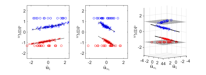
Figure 3: $2$-dimensional projections onto $\mathcal{S}_{1}={\rm span}(\hat{\mathbf{u}}_{1},w_{\textup{MDP}})$ and $\mathcal{S}_{n_{1}}={\rm span}(\hat{\mathbf{u}}_{n_{1}},w_{\textup{MDP}})$ and $3$-dimensional projections onto $\mathcal{S}={\rm span}(\left\{\hat{\mathbf{u}}_{i}\right\}_{i\in\mathcal{D}},w_{\textup{MDP}})$ with $\mathcal{D}=\left\{1,n_{1}\right\}$ of training data $\mathcal{X}$ (class 1: blue circles, class 2: red circles) and independent test data $\mathcal{Y}$ (class 1: blue crosses, class 2: red crosses) under the model in Example 3.

To understand this phenomenon, we focus on the geometric representation of HDLSS data. Jung et al. (2012) showed that in one class case, HDLSS data from strongly spiked covariance model (that is, $\beta_{k}=1$) can asymptotically be decomposed into random and deterministic parts; the random variation remains in ${\rm span}(\mathbf{u}_{1})$, while the deterministic structure (that is, the simplex described in Remark 1) remains in the orthogonal complement of ${\rm span}(\mathbf{u}_{1})$. For sufficiently large $p$, $\hat{\mathbf{u}}_{1}$ explains the most important variation along $\mathbf{u}_{1}$ in the data from both classes, while $\hat{\mathbf{u}}_{2},\ldots,\hat{\mathbf{u}}_{n_{1}-1}$ account for the deterministic simplex with edge length $\sqrt{2}\tau_{1}\sqrt{p}$ for data only from the first class. Then $\hat{\mathbf{u}}_{n_{1}}$ explains remaining variation along $\mathbf{u}_{1}$ in the data from both classes, which is smaller than the variance $\tau_{1}^{2}$ of the first class but larger than the variance $\tau_{2}^{2}$ of the second class. Lastly, $\hat{\mathbf{u}}_{n_{1}+1},\ldots,\hat{\mathbf{u}}_{n-2}$ account for the deterministic simplex with edge length $\sqrt{2}\tau_{2}\sqrt{p}$ for data only from the second class. We emphasize that this result can be obtained with probability $1$. Note that if $\tau_{1}^{2}=\tau_{2}^{2}$, then only $\hat{\mathbf{u}}_{1}$ explains variation along $\mathbf{u}_{1}$ in the data, while the other sample eigenvectors explain the deterministic simplex for data from both classes.

Example 4

Two classes do not have a common leading eigenvector, that is, $\mathbf{u}_{(1),1}\neq\mathbf{u}_{(2),1}$ such that leading eigenvectors of each class form an angle of $\pi/4$, but this time we assume $\tau_{1}^{2}>\tau_{2}^{2}$ instead of $\tau_{1}^{2}=\tau_{2}^{2}$ in Example 2.

As in the previous examples, it turns out that $\hat{\mathbf{u}}_{1}$ estimates the largest variation within the common leading eigenspace $\mathcal{U}$ from the data. However, in this example, the remaining variation may be either larger or smaller than $\tau_{1}^{2}$ in contrast to the other examples. If the remaining variation within $\mathcal{U}$ is smaller than $\tau_{1}^{2}$, then this variation is captured by $\hat{\mathbf{u}}_{n_{1}}$, while $\hat{\mathbf{u}}_{2}$ explains the deterministic simplex of data from the first class. Otherwise, $\hat{\mathbf{u}}_{2}$ captures the remaining variation, while $\hat{\mathbf{u}}_{n_{1}}$ explains the deterministic simplex of data from the first class. The other remaining sample eigenvectors are strongly inconsistent with $\mathcal{U}$. Hence, let $\mathcal{D}=\left\{1,2,n_{1}\right\}$.

In Figure 4, independent test data $\mathcal{Y}$ projected onto $\mathcal{S}_{1}={\rm span}(\hat{\mathbf{u}}_{1},w_{\textup{MDP}})$ and $\mathcal{S}_{n_{1}}={\rm span}(\hat{\mathbf{u}}_{n_{1}},w_{\textup{MDP}})$ are concentrated along lines, but in both subspaces these lines are not parallel to each other. Also, independent test data $\mathcal{Y}$ projected onto $\mathcal{S}_{2}={\rm span}(\hat{\mathbf{u}}_{2},w_{\textup{MDP}})$ are concentrated along lines, which is parallel to $w_{\textup{MDP}}$, but these lines can completely overlap. However, within the $3$-dimensional subspace $\mathcal{S}_{1,n_{1}}={\rm span}(\hat{\mathbf{u}}_{1},\hat{\mathbf{u}}_{n_{1}},w_{\textup{MDP}})$, there are two parallel $2$-dimensional planes respectively including those lines. Similar to Example 2, $\mathcal{Y}_{1}$ is distributed along the direction $P_{\mathcal{S}_{1,n_{1}}}\mathbf{u}_{(1),1}$, while $\mathcal{Y}_{2}$ is distributed along the direction $P_{\mathcal{S}_{1,n_{1}}}\mathbf{u}_{(2),1}$. Thus, these lines are asymptotically contained in $2$-dimensional affine subspaces, that are parallel to $P_{\mathcal{S}_{1,n_{1}}}\mathcal{U}={\rm span}(P_{\mathcal{S}_{1,n_{1}}}\mathbf{u}_{(1),1},P_{\mathcal{S}_{1,n_{1}}}\mathbf{u}_{(2),1})$.

Note that $\hat{\mathbf{u}}_{2}$ instead of $\hat{\mathbf{u}}_{n_{1}}$ can capture the remaining variability within $\mathcal{U}$ depending on the true leading principal components scores of training data $\mathcal{X}$. Then $2$-dimensional parallel affine subspaces can be observed in $\mathcal{S}_{1,2}={\rm span}(\hat{\mathbf{u}}_{1},\hat{\mathbf{u}}_{2},w_{\textup{MDP}})$ instead of $\mathcal{S}_{1,n_{1}}={\rm span}(\hat{\mathbf{u}}_{1},\hat{\mathbf{u}}_{n_{1}},w_{\textup{MDP}})$. However, we can always observe $2$-dimensional parallel affine subspaces in $\mathcal{S}={\rm span}(\left\{\hat{\mathbf{u}}_{i}\right\}_{i\in\mathcal{D}},w_{\textup{MDP}})$.

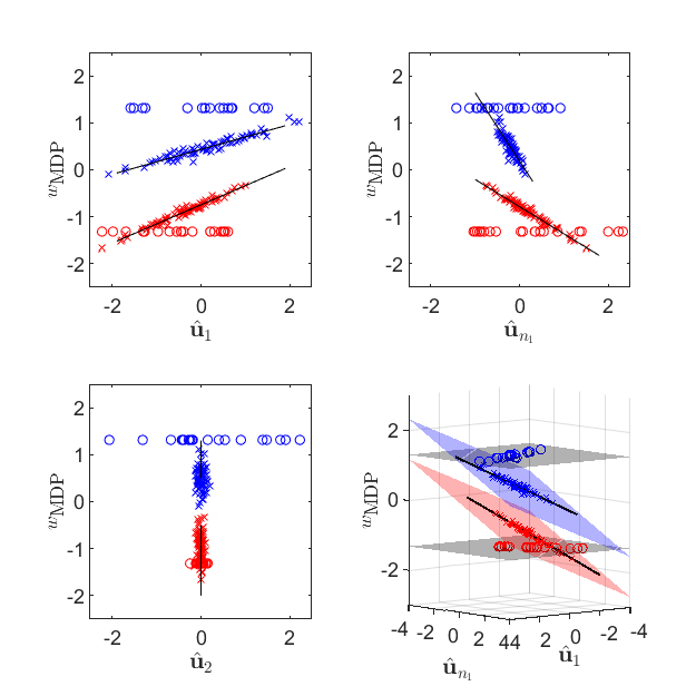
Figure 4: $2$-dimensional projections onto $\mathcal{S}_{1}={\rm span}(\hat{\mathbf{u}}_{1},w_{\textup{MDP}})$, $\mathcal{S}_{2}={\rm span}(\hat{\mathbf{u}}_{2},w_{\textup{MDP}})$ and $\mathcal{S}_{n_{1}}={\rm span}(\hat{\mathbf{u}}_{n_{1}},w_{\textup{MDP}})$ and $3$-dimensional projections onto $\mathcal{S}_{1,n_{1}}={\rm span}(\hat{\mathbf{u}}_{1},\hat{\mathbf{u}}_{n_{1}},w_{\textup{MDP}})$ of training data $\mathcal{X}$ (class 1: blue circles, class 2: red circles) and independent test data $\mathcal{Y}$ (class 1: blue crosses, class 2: red crosses) under the model in Example 4.

The following proposition states that even if $\tau_{1}^{2}>\tau_{2}^{2}$, projections of $\mathcal{Y}$ onto $\mathcal{S}$, which is a low-dimensional subspace of $\mathcal{S}_{X}$, are distributed along two parallel affine subspaces as $p$ increases. However, in this case, $\mathcal{S}$ is not the subspace spanned by the first $m$ eigenvectors of $\mathbf{S}_{W}$ and $w_{\textup{MDP}}$.

Proposition 2

Suppose Assumptions 1—5 hold. Also, assume $\beta_{1}=\beta_{2}=1$, $\tau_{1}^{2}>\tau_{2}^{2}$ and $m_{1}=m_{2}=1$.

• If $m=1$, let $\mathcal{S}={\rm span}(\hat{\mathbf{u}}_{1},\hat{\mathbf{u}}_{n_{1}},w_{\textup{MDP}})$ and $L_{k}=\left\{\mathbf{u}_{1,{\mathcal{S}}}t+\nu_{k}w_{\textup{MDP}}+\bar{X}_{\mathcal{S}}:t\in\mathbb{R}\right\}$

• If $m=2$, let $\mathcal{S}={\rm span}(\hat{\mathbf{u}}_{1},\hat{\mathbf{u}}_{2},\hat{\mathbf{u}}_{n_{1}},w_{\textup{MDP}})$ and $L_{k}=\left\{\mathbf{U}_{1,{\mathcal{S}}}\mathbf{t}+\nu_{k}w_{\textup{MDP}}+\bar{X}_{\mathcal{S}}:\mathbf{t}\in\mathbb{R}^{2}\right\}$

for $k=1,2$ where $\nu_{1}=\kappa_{\textup{MDP}}^{-1}(\eta_{2}(1-\cos^{2}\varphi)\delta^{2}-(\tau_{1}^{2}-\tau_{2}^{2})/n)$ and $\nu_{2}=\kappa_{\textup{MDP}}^{-1}(-\eta_{1}(1-\cos^{2}\varphi)\delta^{2}-(\tau_{1}^{2}-\tau_{2}^{2})/n).$ Then, for any independent observation $Y\in\mathcal{Y}$ and for any $\epsilon>0$,

$$\lim\limits_{p\to\infty}\mathbb{P}\left(\inf\limits_{a\in L_{k}}\|Y_{\mathcal{S}}-a\|>\epsilon|\pi(Y)=k\right)=0$$

for $k=1,2$.

3.2 Characterization of the Signal Subspace $\mathcal{S}$

In Section 3.1, we have seen that there exists a low-dimensional subspace $\mathcal{S}$ such that projections of independent test data $\mathcal{Y}$ onto $\mathcal{S}$ tend to lie on parallel affine subspaces, one for each class. The subspace $\mathcal{S}$ was either ${\rm span}(\hat{\mathbf{u}}_{1},w_{\textup{MDP}})$, ${\rm span}(\hat{\mathbf{u}}_{1},\hat{\mathbf{u}}_{2},w_{\textup{MDP}})$, ${\rm span}(\hat{\mathbf{u}}_{1},\hat{\mathbf{u}}_{n_{1}},w_{\textup{MDP}})$ or ${\rm span}(\hat{\mathbf{u}}_{1},\hat{\mathbf{u}}_{2},\hat{\mathbf{u}}_{n_{1}},w_{\textup{MDP}})$, which was spanned by some sample eigenvectors of $\mathbf{S}_{W}$, which explain the variability within the common leading eigenspace $\mathcal{U}$, and $w_{\textup{MDP}}$.

In this subsection, we characterize the signal subspace $\mathcal{S}$ for general cases where $m_{1}\geq 1$ and $m_{2}\geq 1$. For this, we investigate the asymptotic behavior of sample eigenvalues and eigenvectors of $\mathbf{S}_{W}$. For each $k=1,2$, denote the $n_{k}\times m_{k}$ matrix of the leading $m_{k}$ principal component scores of the $k$th class as $\mathbf{W}_{(k)}=[\sigma_{(k),1}z_{(k),1},\ldots,\sigma_{(k),m_{k}}z_{(k),m_{k}}]$. Also, denote the scaled covariance matrix of the leading $m_{k}$ principal component scores of the $k$th class as

$$\mbox{\boldmath{$\Phi$}}_{k}=\mathbf{W}_{(k)}^{\top}(\mathbf{I}_{n_{k}}-\frac{1}{n_{k}}\mathbf{J}_{n_{k}})\mathbf{W}_{(k)}$$ (3)

where $\mathbf{J}_{n_{k}}$ is the matrix of size $n_{k}\times n_{k}$ whose all entries are $1$. Note that $\mbox{\boldmath{$\Phi$}}_{1}$, $\mbox{\boldmath{$\Phi$}}_{2}$ are symmetric positive definite matrices with probability $1$. Let $\mathbf{W}=[\mathbf{R}_{(1)}\mathbf{W}_{(1)}^{\top}~{}\mathbf{R}_{(2)}\mathbf{W}_{(2)}^{\top}]^{\top}$ and

$$\mbox{\boldmath{$\Phi$}}=\mathbf{W}^{\top}(\mathbf{I}_{n}-\mathbf{J})\mathbf{W}$$ (4)

where $\mathbf{J}=\begin{pmatrix}\frac{1}{n_{1}}\mathbf{J}_{n_{1}}&\mathbf{O}_{n_{1}\times n_{2}}\\ \mathbf{O}_{n_{2}\times n_{1}}&\frac{1}{n_{2}}\mathbf{J}_{n_{2}}\end{pmatrix}$. Finally, let

$$\mbox{\boldmath{$\Phi$}}_{\tau_{1},\tau_{2}}=\begin{pmatrix}\mbox{\boldmath{$\Phi$}}_{1}+\tau_{1}^{2}\mathbf{I}_{m_{1}}&\mbox{\boldmath{$\Phi$}}_{1}^{1/2}\mathbf{R}_{(1)}^{\top}\mathbf{R}_{(2)}\mbox{\boldmath{$\Phi$}}_{2}^{1/2}\\ \mbox{\boldmath{$\Phi$}}_{2}^{1/2}\mathbf{R}_{(2)}^{\top}\mathbf{R}_{(1)}\mbox{\boldmath{$\Phi$}}_{1}^{1/2}&\mbox{\boldmath{$\Phi$}}_{2}+\tau_{2}^{2}\mathbf{I}_{m_{2}}\end{pmatrix}.$$ (5)

Note that $\Phi$ and $\mbox{\boldmath{$\Phi$}}_{\tau_{1},\tau_{2}}$ are also symmetric positive definite matrices with probability $1$. For any square matrix $\mathbf{M}\in\mathbb{R}^{l\times l}$ ($l\in\mathbb{N}$), let $\phi_{i}(\mathbf{M})$ and $v_{i}(\mathbf{M})$ denote the $i$th largest eigenvalue of $\mathbf{M}$ and its corresponding eigenvector, respectively. The following lemma shows asymptotic behavior of sample eigenvalues of $\mathbf{S}_{W}$. Throughout, we assume $\tau_{1}^{2}\geq\tau_{2}^{2}$.

Lemma 3

Suppose Assumptions 1—5 hold. Then, the following hold as $p\to\infty$.

• If $\beta_{1}=\beta_{2}=1$ and $\tau_{1}^{2}=\tau_{2}^{2}=:\tau^{2}$, then conditional to $\mathbf{W}_{(1)}$ and $\mathbf{W}_{(2)}$,

  $$p^{-1}\hat{\lambda}_{i}\xrightarrow{P}\begin{cases}\phi_{i}(\mbox{\boldmath{$\Phi$}})+\tau^{2},&1\leq i\leq m,\\ \tau^{2},&m+1\leq i\leq n-2.\end{cases}$$

• If $\beta_{1}=\beta_{2}=1$ and $\tau_{1}^{2}>\tau_{2}^{2}$, then conditional to $\mathbf{W}_{(1)}$ and $\mathbf{W}_{(2)}$,

  $$p^{-1}\hat{\lambda}_{i}\xrightarrow{P}\begin{cases}\phi_{i}(\mbox{\boldmath{$\Phi$}}_{\tau_{1},\tau_{2}}),&1\leq i\leq k_{0},\\ \tau_{1}^{2},&k_{0}+1\leq i\leq k_{0}+(n_{1}-m_{1}-1),\\ \phi_{i-(n_{1}-m_{1}-1)}(\mbox{\boldmath{$\Phi$}}_{\tau_{1},\tau_{2}}),&k_{0}+(n_{1}-m_{1})\leq i\leq n_{1}+m_{2}-1,\\ \tau_{2}^{2},&n_{1}+m_{2}\leq i\leq n-2,\end{cases}$$

  where $k_{0}$ $(m_{1}\leq k_{0}\leq m_{1}+m_{2})$ is an integer which satisfies $\phi_{k_{0}}(\mbox{\boldmath{$\Phi$}}_{\tau_{1},\tau_{2}})\geq\tau_{1}^{2}\geq\phi_{k_{0}+1}(\mbox{\boldmath{$\Phi$}}_{\tau_{1},\tau_{2}})$ if we denote $\phi_{m_{1}+m_{2}+1}(\mbox{\boldmath{$\Phi$}}_{\tau_{1},\tau_{2}})=0$.

Remark 2

$(i)$ If $\tau_{1}^{2}=\tau_{2}^{2}=:\tau^{2}$, then

$$\phi_{i}(\mbox{\boldmath{$\Phi$}}_{\tau_{1},\tau_{2}})=\begin{cases}\phi_{i}(\mbox{\boldmath{$\Phi$}})+\tau^{2},&1\leq i\leq m,\\ \tau^{2},&m+1\leq i\leq m_{1}+m_{2}.\end{cases}.$$

Thus, Lemma 3 $(i)$ can be seen as a special case of Lemma 3 $(ii)$.

$(ii)$ If $\beta_{1}=\beta_{2}=1$, $\tau_{1}^{2}>\tau_{2}^{2}$ and $m=m_{1}$, then $k_{0}$ in Lemma 3 $(ii)$ is $m_{1}$ with probability $1$ by Weyl’s inequality.

Lemma 3 shows that for the case of strong spikes $(\beta_{1}=\beta_{2}=1)$, the asymptotic behavior of sample eigenvalues of $\mathbf{S}_{W}$ is quite different depending on whether both covariance matrices have equal tail eigenvalues or unequal tail eigenvalues. If $\tau_{1}^{2}=\tau_{2}^{2}$, then the first $m$ sample eigenvalues explain true leading principal component scores of both classes, while the other sample eigenvalues do not. In contrast, if $\tau_{1}^{2}\neq\tau_{2}^{2}$, we observe a counter-intuitive phenomenon that some non-leading sample eigenvalues can explain true leading principal component scores instead of some leading sample eigenvalues.

The following lemma gives the limiting angle between $\hat{\mathbf{u}}_{i}$ and the common leading eigenspace $\mathcal{U}$.

Lemma 4

Suppose Assumptions 1—5 hold. Then, the following hold as $p\to\infty$.

$(i)$ If $\beta_{1}=\beta_{2}=1$ and $\tau_{1}^{2}=\tau_{2}^{2}=:\tau^{2}$, then conditional to $\mathbf{W}_{(1)}$ and $\mathbf{W}_{(2)}$,

$$\cos{\left(\mbox{Angle}{(\hat{\mathbf{u}}_{i},\mathcal{U})}\right)}\xrightarrow{P}\begin{cases}C_{i},&1\leq i\leq m,\\ 0,&m+1\leq i\leq n-2\end{cases}$$

where

$$C_{i}=\sqrt{\frac{\phi_{i}(\mbox{\boldmath{$\Phi$}})}{\phi_{i}(\mbox{\boldmath{$\Phi$}})+\tau^{2}}}>0.$$ (6)

$(ii)$ If $\beta_{1}=\beta_{2}=1$, $\tau_{1}^{2}>\tau_{2}^{2}$ and $m=m_{1}$, then conditional to $\mathbf{W}_{(1)}$ and $\mathbf{W}_{(2)}$,

$$\cos{\left(\mbox{Angle}{(\hat{\mathbf{u}}_{i},\mathcal{U})}\right)}\xrightarrow{P}\begin{cases}D_{i},&1\leq i\leq m_{1},\\ 0,&m_{1}+1\leq i\leq n_{1}-1,\\ D_{i-(n_{1}-m_{1}-1)},&n_{1}\leq i\leq n_{1}+m_{2}-1,\\ 0,&n_{1}+m_{2}\leq i\leq n-2\end{cases}$$

where

$$D_{i}=\sqrt{\frac{\|\sum_{k=1}^{2}\mathbf{R}_{(k)}\mbox{\boldmath{$\Phi$}}_{k}^{1/2}\tilde{v}_{ik}(\mbox{\boldmath{$\Phi$}}_{\tau_{1},\tau_{2}})\|^{2}}{\phi_{i}(\mbox{\boldmath{$\Phi$}}_{\tau_{1},\tau_{2}})}}>0.$$ (7)

and $v_{i}(\mbox{\boldmath{$\Phi$}}_{\tau_{1},\tau_{2}})=(\tilde{v}_{i1}(\mbox{\boldmath{$\Phi$}}_{\tau_{1},\tau_{2}})^{\top},\tilde{v}_{i2}(\mbox{\boldmath{$\Phi$}}_{\tau_{1},\tau_{2}})^{\top})^{\top}$ with $\tilde{v}_{i1}(\mbox{\boldmath{$\Phi$}}_{\tau_{1},\tau_{2}})\in\mathbb{R}^{m_{1}}$ and $\tilde{v}_{i2}(\mbox{\boldmath{$\Phi$}}_{\tau_{1},\tau_{2}})\in\mathbb{R}^{m_{2}}$.

$(iii)$ If $\beta_{1}=\beta_{2}=1$, $\tau_{1}^{2}>\tau_{2}^{2}$ and $m>m_{1}$, then conditional to $\mathbf{W}_{(1)}$ and $\mathbf{W}_{(2)}$,

$$\cos{\left(\mbox{Angle}{(\hat{\mathbf{u}}_{i},\mathcal{U})}\right)}\xrightarrow{P}\begin{cases}D_{i},&1\leq i\leq k_{0},\\ 0,&k_{0}+1\leq i\leq k_{0}+(n_{1}-m_{1}-1),\\ D_{i-(n_{1}-m_{1}-1)}I(k_{0}<i-(n_{1}-m_{1}-1)),&k_{0}+(n_{1}-m_{1})\leq i\leq n_{1}+m_{2}-1,\\ 0,&n_{1}+m_{2}\leq i\leq n-2\end{cases}$$

where $k_{0}$ is defined in Lemma 3 $(ii)$ and $D_{i}$ is defined in (7).

From Lemmas 3 and 4, we summarize the asymptotic behavior of sample eigenvectors for general cases where $m_{1}\geq 1$ and $m_{2}\geq 1$.

• If $\tau_{1}^{2}=\tau_{2}^{2}$, then the first $m$ leading eigenvectors of $\mathbf{S}_{W}$ explain the variation within the common leading eigenspace $\mathcal{U}$. The other sample eigenvectors are asymptotically orthogonal to $\mathcal{U}$, which implies that these eigenvectors do not capture the variability within $\mathcal{U}$. In this case, the first $m$ sample eigenvectors are needed to explain the variation within $\mathcal{U}$.

• If $\tau_{1}^{2}>\tau_{2}^{2}$, then some non-leading eigenvectors of $\mathbf{S}_{W}$ may capture the variability within $\mathcal{U}$ instead of some leading eigenvectors, in contrast to the case of $\tau_{1}^{2}=\tau_{2}^{2}$.

  • If $m=m_{1}$, then $\hat{\mathbf{u}}_{1},\ldots,\hat{\mathbf{u}}_{m}$ explain the most important variation within $\mathcal{U}$, while $\hat{\mathbf{u}}_{n_{1}},\ldots,\hat{\mathbf{u}}_{n_{1}+m_{2}-1}$ explain the remaining variation within $\mathcal{U}$, which is smaller than the variance $\tau_{1}^{2}$ of the first class but larger than the variance $\tau_{2}^{2}$ of the second class. The other sample eigenvectors do not explain the variability. That is, $(m_{1}+m_{2})$ sample eigenvectors are needed to explain the variation within $\mathcal{U}$.

  • If $m>m_{1}$, then $\hat{\mathbf{u}}_{1},\ldots,\hat{\mathbf{u}}_{k_{0}}$ explain the most important variation within $\mathcal{U}$, while $\hat{\mathbf{u}}_{k_{0}+(n_{1}-m_{1})},\ldots,\hat{\mathbf{u}}_{n_{1}+m_{2}-1}$ explain the remaining variation, where $k_{0}$ is defined in Lemma 3 $(ii)$. The other sample eigenvectors do not contribute to capture the variability within $\mathcal{U}$. It implies that $(m_{1}+m_{2})$ eigenvectors are needed to explain the variation within $\mathcal{U}$. However, $k_{0}$ $(m_{1}\leq k_{0}\leq m_{1}+m_{2})$ is a random number depending on true leading principal component scores $\mathbf{W}_{(1)}$ and $\mathbf{W}_{(2)}$, thus we can not identify $k_{0}$ unless we know true leading principal component scores. If $P(k_{0}=i)>0$ for $m_{1}\leq i\leq m_{1}+m_{2}$, then $(m_{1}+2m_{2})$ sample eigenvectors, which are $\hat{\mathbf{u}}_{1},\ldots,\hat{\mathbf{u}}_{m_{1}+m_{2}}$ and $\hat{\mathbf{u}}_{n_{1}},\ldots,\hat{\mathbf{u}}_{n_{1}+m_{2}-1}$, are needed to explain the variation within $\mathcal{U}$.

Remark 3

Under the one-component covariance model in Example 4, $P(k_{0}=i)$ $(i=1,2)$ depends on the magnitude of signals $\sigma_{(1),1}^{2}$ and $\sigma_{(2),1}^{2}$, the tail eigenvalues $\tau_{1}^{2}$ and $\tau_{2}^{2}$, and the angle between $\mathbf{u}_{(1),1}$ and $\mathbf{u}_{(2),1}$. See Figure 5.

Figure 5: Under the model in Example 4, we assume $(\sigma_{(1),1}^{2},\sigma_{(2),1}^{2})=(2,1)$, $(\tau_{1}^{2},\tau_{2}^{2})=(40,20)$ and $\cos{(\mbox{Angle}{(\mathbf{u}_{(1),1},\mathbf{u}_{(2),1})})}=1/2$. $P(k_{0}=1)$ is empirically estimated using $(n_{1},n_{2})=(20,20)$ with Gaussian assumption. The first/second/last panel shows the estimates with different $\tau_{2}^{2}$/$\sigma_{(2),1}^{2}$/$\mbox{Angle}{(\mathbf{u}_{(1),1},\mathbf{u}_{(2),1})}$ while the other parameters are fixed, respectively.

We define an index set $\mathcal{D}\subset\left\{1,\ldots,n-2\right\}$ for general cases where $m_{1}\geq 1$ and $m_{2}\geq 1$. Let $i\in\mathcal{D}$ if and only if there exists $\epsilon>0$ such that $\lim\limits_{p\to\infty}P(\cos{(\mbox{Angle}{(\hat{\mathbf{u}}_{i},\mathcal{U})})}>\epsilon)>0$. In contrast, $i\notin\mathcal{D}$ if and only if $\hat{\mathbf{u}}_{i}$ is strongly inconsistent with the common leading eigenspace $\mathcal{U}$ in the sense that $\mbox{Angle}(\hat{\mathbf{u}}_{i},\mathcal{U})\xrightarrow{P}\pi/2$ as $p\to\infty$. In other words, $\hat{\mathbf{u}}_{i}$ with $i\notin\mathcal{D}$ is a noisy direction which does not capture important variability within the common leading eigenspace $\mathcal{U}$, while $\hat{\mathbf{u}}_{i}$ with $i\in\mathcal{D}$ may explain important variability. From Lemma 4, we characterize $\mathcal{D}$ for general cases where $m_{1}\geq 1$ and $m_{2}\geq 1$.

Proposition 5

Suppose Assumptions 1—5 hold. Also, assume $\beta_{1}=\beta_{2}=1$.

$(i)$ If $\tau_{1}^{2}=\tau_{2}^{2}$, then $\mathcal{D}=\left\{1,\ldots,m\right\}$.

$(ii)$ If $\tau_{1}^{2}>\tau_{2}^{2}$ and $m=m_{1}$, then $\mathcal{D}=\left\{1,\ldots,m_{1},n_{1},\ldots,n_{1}+m_{2}-1\right\}$.

$(iii)$ If $\tau_{1}^{2}>\tau_{2}^{2}$, $m>m_{1}$ and $P(k_{0}=i)>0$ for all $m_{1}\leq i\leq m_{1}+m_{2}$, then $\mathcal{D}=\left\{1,\ldots,m_{1}+m_{2},n_{1},\ldots,n_{1}+m_{2}-1\right\}$.

For the case of weak spikes ($\beta_{1},\beta_{2}<1$), we have $\mathcal{U}=\mathbf{0}_{p}$ in Section 2 and $\mathcal{D}=\emptyset$. In this case, the sample eigenvectors $\hat{\mathbf{u}}_{1},\ldots,\hat{\mathbf{u}}_{n-2}$ are strongly inconsistent with the leading eigenspace of the $k$th class $\mathcal{U}_{(k)}$ $(k=1,2)$; see Appendix C for details. We summarize $\mathcal{D}$ in Table 1 for each case. For the cases where only one class has meaningfully diverging components while the other class does not (that is, $(i)$ $\beta_{1}=1,\beta_{2}<1$ and $(ii)$ $\beta_{1}<1,\beta_{2}=1$), the results are given in Appendix B.

Case	$\beta_{1},\beta_{2}$	Condition	$\mathcal{D}$	$|\mathcal{D}|$
Weak spikes	$\beta_{1}<1$	-	$\emptyset$	$0$
	$\beta_{2}<1$
Strong spikes		$\tau_{1}^{2}=\tau_{2}^{2}$	$\left\{1,\ldots,m\right\}$	$m$
	$\beta_{1}=1$	$\tau_{1}^{2}>\tau_{2}^{2}$	$\left\{1,\ldots,m_{1},n_{1},\ldots,n_{1}+m_{2}-1\right\}$	$m_{1}+m_{2}$
	$\beta_{2}=1$	$m=m_{1}$
		$\tau_{1}^{2}>\tau_{2}^{2}$	$\left\{1,\ldots,m_{1}+m_{2},n_{1},\ldots,n_{1}+m_{2}-1\right\}$	$m_{1}+2m_{2}$
		$m>m_{1}$

Table 1: The index set $\mathcal{D}$ for each case.

In general, we define the signal subspace $\mathcal{S}$ as

$$\mathcal{S}={\rm span}(\left\{\hat{\mathbf{u}}_{i}\right\}_{i\in\mathcal{D}},w_{\textup{MDP}}),$$ (8)

which is obtained by removing the noisy directions in the sample space $\mathcal{S}_{X}$.

Remark 4

For the case of strong spikes with unequal tail eigenvalues $(\beta_{1}=\beta_{2}=1,\tau_{1}^{2}\neq\tau_{2}^{2})$, let $\mathcal{D}^{\prime}=\left\{1,\ldots,k_{0},k_{0}+(n_{1}-m_{1}),\ldots,n_{1}+m_{2}-1\right\}$ for any given training data $\mathcal{X}$ where $k_{0}$ is defined in Lemma 3. Note that $|\mathcal{D}^{\prime}|=m_{1}+m_{2}$. Also, let $\mathcal{S}^{\prime}={\rm span}(\left\{\hat{\mathbf{u}}_{i}\right\}_{i\in\mathcal{D}^{\prime}},w_{\textup{MDP}})$ so that $\mathcal{S}=\mathcal{S}^{\prime}\oplus{\rm span}(\left\{\hat{\mathbf{u}}_{i}\right\}_{i\in\mathcal{D}\setminus\mathcal{D}^{\prime}})$. In fact, the subspace of interest is $\mathcal{S}^{\prime}$, which is obtained by further removing a noisy subspace ${\rm span}(\left\{\hat{\mathbf{u}}_{i}\right\}_{i\in\mathcal{D}\setminus\mathcal{D}^{\prime}})$ from $\mathcal{S}$. However, if $P(k_{0}=i)>0$ for all $m_{1}\leq i\leq m_{1}+m_{2}$, then it is impossible to determine $\mathcal{S}^{\prime}$ unless we know true leading principal component scores.

3.3 Main Theorem

In this subsection, we extend Propositions 1 and 2 to the general cases where $m_{1}\geq 1$ and $m_{2}\geq 1$. We confirm that projections of $\mathcal{Y}$ onto $\mathcal{S}$ in (8), which is a low-dimensional subspace of the sample space $\mathcal{S}_{X}$, are distributed along parallel affine subspaces, one for each class, and that those affine subspaces do not coincide. Recall that $\kappa_{\textup{MDP}}$ is the training data piling distance defined in (2).

Theorem 6

Suppose Assumptions 1—5 hold. Let $\mathcal{S}={\rm span}(\left\{\hat{\mathbf{u}}_{i}\right\}_{i\in\mathcal{D}},w_{\textup{MDP}})$ with $\mathcal{D}$ be given in Table 1 for each case. Also, let

$$L_{k}=\left\{\mathbf{U}_{1,{\mathcal{S}}}\mathbf{t}+\nu_{k}w_{\textup{MDP}}+\bar{X}_{\mathcal{S}}:\mathbf{t}\in\mathbb{R}^{m}\right\}$$

for $k=1,2$ where

$$\nu_{1}=\kappa_{\textup{MDP}}^{-1}\left(\eta_{2}(1-\cos^{2}\varphi)\delta^{2}-(\tau_{1}^{2}-\tau_{2}^{2})/n\right)$$

and

$$\nu_{2}=\kappa_{\textup{MDP}}^{-1}\left(-\eta_{1}(1-\cos^{2}\varphi)\delta^{2}-(\tau_{1}^{2}-\tau_{2}^{2})/n\right)$$

Then for any independent observation $Y\in\mathcal{Y}$ and for any $\epsilon>0$,

$$\lim\limits_{p\to\infty}\mathbb{P}\left(\inf\limits_{a\in L_{k}}\|Y_{\mathcal{S}}-a\|>\epsilon|\pi(Y)=k\right)=0$$

for $k=1,2$. Recall that if $m=0$, then $L_{k}=\nu_{k}w_{\textup{MDP}}+\bar{X}_{\mathcal{S}}$ for $k=1,2$ and $\cos^{2}\varphi=0$.

Write the projections of $\mathbf{u}_{(k),i}$ $(k=1,2)$ onto a subspace $\mathcal{S}$ of $\mathbb{R}^{p}$ as $\mathbf{u}_{(k),i,\mathcal{S}}=P_{\mathcal{S}}\mathbf{u}_{(k),i}$ and write $\mathbf{U}_{(k),1,\mathcal{S}}=[\mathbf{u}_{(k),1,\mathcal{S}},\ldots,\mathbf{u}_{(k),m_{k},\mathcal{S}}]$ for $k=1,2$.

Remark 5

$(i)$ For the case of weak spikes ($\beta_{1}<1$ and $\beta_{2}<1$), projections of $\mathcal{Y}_{1}$ and $\mathcal{Y}_{2}$ are asymptotically piled on two distinct points on $w_{\textup{MDP}}$, one for each class. $(ii)$ For the case of strong spikes ($\beta_{1}=1$ and $\beta_{2}=1$), projections of $\mathcal{Y}_{1}$ are distributed along an $m_{1}$-dimensional affine subspace $L_{1}^{\prime}$, which is parallel to ${\rm span}(\mathbf{U}_{(1),1,\mathcal{S}})$, while projections of $\mathcal{Y}_{2}$ are distributed along an $m_{2}$-dimensional affine subspace $L_{2}^{\prime}$, which is parallel to ${\rm span}(\mathbf{U}_{(2),1,\mathcal{S}})$. For each $k=1,2$, the $m$-dimensional affine subspace $L_{k}$ contains $L_{k}^{\prime}$.

Theorem 6 tells that independent test data are asymptotically distributed along parallel $m$-dimensional affine subspaces $L_{1}$ and $L_{2}$ in $\mathcal{S}$. It implies that if we find a direction $w\in\mathcal{S}$ such that $w$ is asymptotically orthogonal to $L_{1}$ and $L_{2}$, then $P_{w}\mathcal{Y}$ yields the second data piling and in turn achieves perfect classification of independent test data.

For the case of strong spikes, if $\tau_{1}^{2}=\tau_{2}^{2}$, then $\dim{\mathcal{S}}-m=1$, which implies that a second data piling direction in $\mathcal{S}$ is asymptotically unique. In contrast, if $\tau_{1}^{2}>\tau_{2}^{2}$ then $\dim{\mathcal{S}}-m\geq 1$, which implies that there may be a multi-dimensional subspace in $\mathcal{S}$ such that any direction in this subspace yields second data piling. Hence, for all cases, we can conclude that there exists a direction $w\in\mathcal{S}$ which yields second data piling. Meanwhile, a direction $w\in\mathcal{S}_{X}\setminus\mathcal{S}$ also yields second data piling since this direction is asymptotically orthogonal to the common leading eigenspace $\mathcal{U}$, resulting in projections of $\mathcal{Y}_{1}$ and $\mathcal{Y}_{2}$ converge to a same location. Among these second data piling directions, we will find a second maximal data piling direction, which provides asymptotic maximal distance between the two piles of independent test data, in the following sections.

4 Ridged Discriminant Directions and Second Maximal Data Piling

In this section, we reveal the relationship between a ridged linear discriminant vector and the second data piling phenomenon under various heterogeneous covariance assumptions. For the case of weak spikes, we will show that $w_{\textup{MDP}}$, which is a ridgeless estimator in the context of linear classification, is in fact a second maximal data piling direction for independent test data. In contrast, for the case of strong spikes with equal tail eigenvalues, we will show that a negatively ridged linear discriminant vector, projected onto $\mathcal{S}$ defined in Section 3, not only yields second data piling of independent test data, but also is a second maximal data piling direction.

Write a ridged linear discriminant vector $w_{\alpha}$,

$${w}_{\alpha}\varpropto\alpha_{p}(\mathbf{S}_{W}+\alpha_{p}\mathbf{I}_{p})^{-1}\mathbf{d}=\sum\limits_{i=1}^{n-2}\frac{\alpha_{p}}{\hat{\lambda}_{i}+\alpha_{p}}\hat{\mathbf{u}}_{i}\hat{\mathbf{u}}_{i}^{\top}\mathbf{d}+\hat{\mathbf{U}}_{2}\hat{\mathbf{U}}_{2}^{\top}\mathbf{d},$$ (9)

satisfying $\|w_{\alpha}\|=1$ where $\alpha_{p}=\alpha p$ for a ridge parameter $\alpha\in[-\infty,\infty]$. Note that allowing negative values of the ridge parameter can yield ill-posed problems since $\mathbf{S}_{W}+\alpha_{p}\mathbf{I}_{p}$ may be rank-deficit. We observe that the ridged linear discriminant vector $w_{\alpha}$ concentrates toward $\mathcal{S}$, defined in (8), in high dimensions under heterogeneous covariance assumptions.

Theorem 7

Suppose Assumptions 1—5 hold. Let $\mathcal{S}={\rm span}(\left\{\hat{\mathbf{u}}_{i}\right\}_{i\in\mathcal{D}},w_{\textup{MDP}})$ with $\mathcal{D}$ be given in Table 1 for each case. For any $\alpha\in\mathbb{R}\setminus\left\{-\tau_{1}^{2},-\tau_{2}^{2}\right\}$ for which (9) is defined,

$${\rm Angle}{(w_{\alpha},\mathcal{S})}\xrightarrow{P}0$$

as $p\to\infty$.

Based on this, we consider removing noise terms in $w_{\alpha}$ and define a projected ridged linear discriminant vector $v_{\alpha}$,

$$v_{\alpha}\varpropto\sum\limits_{i\in\mathcal{D}}\frac{\alpha_{p}}{\hat{\lambda}_{i}+\alpha_{p}}\hat{\mathbf{u}}_{i}\hat{\mathbf{u}}_{i}^{\top}\mathbf{d}+\hat{\mathbf{U}}_{2}\hat{\mathbf{U}}_{2}^{\top}\mathbf{d}$$ (10)

satisfying $\|v_{\alpha}\|=1$. Note that $v_{\alpha}$ is $P_{\mathcal{S}}w_{\alpha}/\|P_{\mathcal{S}}w_{\alpha}\|$ for almost all $\alpha\in\mathbb{R}$ except when $\alpha=-\hat{\lambda}_{i}/p$ for $1\leq i\leq n-2$. Also, for the case of weak spikes, $\mathcal{D}=\emptyset$ and $v_{\alpha}$ is $w_{\textup{MDP}}$ for any $\alpha\in\mathbb{R}$. If $\mbox{\boldmath{$\Sigma$}}_{(1)}=\mbox{\boldmath{$\Sigma$}}_{(2)}$ with $m$ strong spikes, then $\mathcal{D}=\left\{1,\ldots,m\right\}$ and

$$v_{\alpha}\varpropto\sum\limits_{i=1}^{m}\frac{\alpha_{p}}{\hat{\lambda}_{i}+\alpha_{p}}\hat{\mathbf{u}}_{i}\hat{\mathbf{u}}_{i}^{\top}\mathbf{d}+\hat{\mathbf{U}}_{2}\hat{\mathbf{U}}_{2}^{\top}\mathbf{d},$$ (11)

which is consistent with the definition of the projected ridged linear discriminant vector in Chang et al. (2021). They showed that if $\mbox{\boldmath{$\Sigma$}}_{(1)}=\mbox{\boldmath{$\Sigma$}}_{(2)}$, then $v_{\alpha}$ is a second maximal data piling direction when $\alpha=\hat{\alpha}$, where $\hat{\alpha}$ is any HDLSS-consistent estimator of $-\tau^{2}$ (that is, $\hat{\alpha}\xrightarrow{P}-\tau^{2}$ as $p\to\infty$). In this section, we generalize the results of Chang et al. (2021) for the case where two populations have heterogeneous covariance matrices.

4.1 The Case of Weak Spikes

In this subsection, we first assume that $\beta_{1}<1$ and $\beta_{2}<1$. For this case, we have seen in Theorem 6 that projections of $\mathcal{Y}_{1}$ and $\mathcal{Y}_{2}$ onto $w_{\textup{MDP}}$ are asymptotically piled on two distinct points, one for each class. It implies that independent test data from weakly correlated populations are asymptotically piled on $w_{\textup{MDP}}$, even if both classes have heterogeneous leading eigenspaces or unequal tail eigenvalues.

Theorem 8

Suppose Assumptions 1—5 hold and assume $\beta_{1},\beta_{2}<1$. For any independent observation $Y$,

$$\frac{1}{\sqrt{p}}v_{\alpha}^{\top}(Y-\bar{X})\xrightarrow{P}\begin{cases}\kappa_{0}^{-1}(\eta_{2}\delta^{2}-(\tau_{1}^{2}-\tau_{2}^{2})/n),&\pi(Y)=1,\\ \kappa_{0}^{-1}(-\eta_{1}\delta^{2}-(\tau_{1}^{2}-\tau_{2}^{2})/n),&\pi(Y)=2\end{cases}$$ (12)

for any $\alpha\in\mathbb{R}$ as $p\to\infty$ where $\kappa_{0}$ is the probability limit of $\kappa_{\textup{MDP}}$ defined in (2). Note that in this case, $v_{\alpha}$ for any $\alpha\in\mathbb{R}$ is $w_{\textup{MDP}}$.

See (67) in Appendix D for the definition of $\kappa_{0}$.

For this case, any sequence $\left\{w\right\}\in\mathfrak{W}_{X}$ is a sequence of second data piling directions, since projections of independent test data from the same class converge to a single point in the sample space $\mathcal{S}_{X}$. Note that $w_{\textup{MDP}}$ gives a meaningful distance between the two piles of independent test data, while the sample eigenvector $\hat{\mathbf{u}}_{i}$ ($1\leq i\leq n-2$) does not. Then it is obvious that $w_{\textup{MDP}}$ is a second maximal data piling direction.

Theorem 9

Suppose Assumptions 1—5 hold assume $\beta_{1},\beta_{2}<1$.

• For any given $\left\{w\right\}\in\mathcal{A}$, there exists a sequence $\left\{v\right\}\in\mathfrak{W}_{X}$ such that $\|w-v\|\xrightarrow{P}0$ as $p\to\infty$.

• For any $\left\{w\right\}\in\mathcal{A}$ such that $D(w)$ exists, $\left\{w\right\}\in\mathcal{A}$ is a sequence of second maximal data piling directions if and only if $\|w-w_{\textup{MDP}}\|\xrightarrow{P}0$ as $p\to\infty$.

From (12), we can check that the original maximal data piling classification rule (Ahn and Marron, 2010),

$$\phi_{\textup{MDP}}(Y;\mathcal{X})=\begin{cases}1,&w_{\textup{MDP}}^{\top}(Y-\bar{X})\geq 0,\\ 2,&w_{\textup{MDP}}^{\top}(Y-\bar{X})<0,\end{cases}$$ (13)

achieves perfect classification if $\tau_{1}^{2}=\tau_{2}^{2}$. However, if $\tau_{1}^{2}\neq\tau_{2}^{2}$, then $\phi_{\textup{MDP}}$ may fail to achieve perfect classification, since the total mean threshold in $\phi_{\textup{MDP}}$ should be adjusted by the bias term in (12). It implies that correct classification rates of each class using $\phi_{\textup{MDP}}$ converge to either $1$ or $0$ as $p$ increases. In the following, we provide a bias-corrected classification rule using $w_{\textup{MDP}}$ to achieve perfect classification even if $\tau_{1}^{2}\neq\tau_{2}^{2}$.

Bias-corrected maximal data piling classification rule

We define the bias-corrected maximal data piling classification rule as

$$\phi_{\textup{b-MDP}}(Y;\mathcal{X})=\begin{cases}1,&p^{-1/2}w_{\textup{MDP}}^{\top}(Y-\bar{X})-(\hat{\alpha}_{1}-\hat{\alpha}_{2})/(n\kappa_{\textup{MDP}})\geq 0,\\ 2,&p^{-1/2}w_{\textup{MDP}}^{\top}(Y-\bar{X})-(\hat{\alpha}_{1}-\hat{\alpha}_{2})/(n\kappa_{\textup{MDP}})<0,\end{cases}$$ (14)

where $\hat{\alpha}_{k}$ is an HDLSS-consistent estimator of $-\tau_{k}^{2}$ for $k=1,2$. From (12), we can check that perfect classification of independent test data is possible using $\phi_{\textup{b-MDP}}$ when $\beta_{1},\beta_{2}<1$.

For the case of $\tau_{1}^{2}=\tau_{2}^{2}$, Hall et al. (2005) showed that Support Vector Machine (SVM) (Vapnik, 1995) and Distance Weighted Discrimination (DWD) (Marron et al., 2007) achieve perfect classification of independent test data under proper conditions. Similarly, weighted Distance Weighted Discrimination (wDWD) (Qiao et al., 2010) also achieves perfect classification under the HDLSS asymptotic regime. However, if $\tau_{1}^{2}\neq\tau_{2}^{2}$, then these classifiers can also suffer from similar problems with $\phi_{\textup{MDP}}$ due to the bias term in (12). We have shown that $w_{\textup{MDP}}$ can achieve perfect classification for independent test data with bias-correction even if $\tau_{1}^{2}\neq\tau_{2}^{2}$.

4.2 The Case of Strong Spikes with Equal Tail Eigenvalues

In this subsection, we assume that $\beta_{1}=\beta_{2}=1$ and $\tau_{1}^{2}=\tau_{2}^{2}=:\tau^{2}$. In this case, recall that $\mathcal{S}$ is the subspace spanned by the first $m$ sample eigenvectors and $w_{\textup{MDP}}$, that is, ${\rm span}(\hat{\mathbf{u}}_{1},\ldots,\hat{\mathbf{u}}_{m},w_{\textup{MDP}})$ and $\dim{\mathcal{S}}-m=1$. Hence, a second data piling direction in $\mathcal{S}$ is asymptotically unique.

Theorem 6 implies that second data piling occurs when a direction $w\in\mathcal{S}$ is asymptotically orthogonal to the common leading eigenspace $\mathcal{U}$ if $\beta_{1}=\beta_{2}=1$. Theorem 10 confirms that for $\hat{\alpha}$ chosen as an HDLSS-consistent estimator of $-\tau^{2}$, $v_{\hat{\alpha}}$ is such a direction, even if two populations do not have a common covariance matrix.

Theorem 10

Suppose Assumptions 1—5 hold and assume $\beta_{1}=\beta_{2}=1$ and $\tau_{1}^{2}=\tau_{2}^{2}$. For $\hat{\alpha}$ chosen as an HDLSS-consistent estimator of $-\tau^{2}$, $\mbox{Angle}{(v_{\hat{\alpha}},\mathbf{u}_{i,\mathcal{S}})}\xrightarrow{P}\pi/2$ as $p\to\infty$ for $1\leq i\leq m$.

From Theorem 6 and Theorem 10, $v_{\hat{\alpha}}$ is asymptotically orthogonal to both of $L_{1}$ and $L_{2}$ defined in Theorem 6. We conclude that both of $P_{v_{\hat{\alpha}}}\mathcal{Y}_{1}$ and $P_{v_{\hat{\alpha}}}\mathcal{Y}_{2}$ asymptotically pile on a single point.

We remark that $v_{\hat{\alpha}}$ can be obtained purely from the training data $\mathcal{X}$. Note that $\hat{\alpha}$ can be estimated purely from the sample eigenvalues of $\mathbf{S}_{W}$ since $\hat{\lambda}_{i}/p\xrightarrow{P}\tau^{2}$ for $m+1\leq i\leq n-2$ as $p\to\infty$ (see Lemma 3). From now on, we fix

$$\hat{\alpha}=-\frac{1}{n-m-2}\sum_{i=m+1}^{n-2}\frac{\hat{\lambda}_{i}}{p}.$$ (15)

In order to achieve perfect classification of independent test data, the two piles of $P_{v_{\hat{\alpha}}}\mathcal{Y}_{1}$ and $P_{v_{\hat{\alpha}}}\mathcal{Y}_{2}$ should also be apart from each other. Theorem 11 shows that projections of $\mathcal{Y}_{1}$ and $\mathcal{Y}_{2}$ onto $v_{\hat{\alpha}}$ are also asymptotically piled on two distinct points, one for each class.

Theorem 11

Suppose Assumptions 1—5 hold and assume $\beta_{1}=\beta_{2}=1$ and $\tau_{1}^{2}=\tau_{2}^{2}$. For any independent observation $Y$,

$$\frac{1}{\sqrt{p}}v_{\hat{\alpha}}^{\top}(Y-\bar{X})\xrightarrow{P}\begin{cases}\gamma(\eta_{2}(1-\cos^{2}\varphi)\delta^{2}),&\pi(Y)=1,\\ \gamma(-\eta_{1}(1-\cos^{2}\varphi)\delta^{2}),&\pi(Y)=2\end{cases}$$ (16)

as $p\to\infty$ where $\gamma$ is a strictly positive random variable depending on the true principal component scores of $\mathcal{X}$.

See (66) in Appendix D for the definition of $\gamma$.

Recall that we write the collection of sequences of second data piling directions as $\mathcal{A}$. Chang et al. (2021) showed that if $\mbox{\boldmath{$\Sigma$}}_{(1)}=\mbox{\boldmath{$\Sigma$}}_{(2)}$ with $m$ strong spikes, then $\mathcal{A}$ is equivalent to a collection of sequences of directions which is asymptotically orthogonal to the common leading eigenspace $\mathcal{U}$, that is,

$$\mathcal{A}=\left\{\left\{w\right\}\in\mathfrak{W}_{X}:w^{\top}\mathbf{u}_{i}\xrightarrow{P}0,1\leq i\leq m\text{ as }p\to\infty\right\}.$$

This fact can be shown similarly for the case of $\mbox{\boldmath{$\Sigma$}}_{(1)}\neq\mbox{\boldmath{$\Sigma$}}_{(2)}$ (see Theorem 3.3 of Chang et al. (2021)).

Theorem 12 shows that $\left\{w\right\}\in\mathcal{A}$ is asymptotically close to a sequence $\left\{v\right\}$ such that $v$ is in the subspace spanned by $v_{\hat{\alpha}}$ and the sample eigenvectors which are strongly inconsistent with $\mathcal{U}$, that is, $\left\{\hat{\mathbf{u}}_{i}\right\}_{i=m+1}^{n-2}$. Among sequences of second data piling directions, note that $v_{\hat{\alpha}}$ provides a meaningful distance between the two piles of independent test data, while $\hat{\mathbf{u}}_{i}$ ($m+1\leq i\leq n-2$) does not, since independent test data tend to be distributed in $\mathcal{S}$, which is orthogonal to $\hat{\mathbf{u}}_{i}$ for $m+1\leq i\leq n-2$, as $p$ increases. This naturally leads to the conclusion that $v_{\hat{\alpha}}$ is a second maximal data piling direction. It can also be seen that a ‘closest’ direction to $w_{\textup{MDP}}$ among second data piling directions is a second maximal data piling direction.

Theorem 12

Suppose Assumptions 1—5 hold and assume $\beta_{1}=\beta_{2}=1$ and $\tau_{1}^{2}=\tau_{2}^{2}$.

• For any given $\left\{w\right\}\in\mathcal{A}$, there exists a sequence $\left\{v\right\}\in\mathcal{B}$ such that $\|w-v\|\xrightarrow{P}0$ as $p\to\infty$, where

  $$\mathcal{B}=\left\{\left\{v\right\}\in\mathfrak{W}_{X}:v\in{\rm span}(v_{\hat{\alpha}})\oplus{\rm span}(\left\{\hat{\mathbf{u}}_{i}\right\}_{i=m+1}^{n-2})\right\}$$

• For any $\left\{w\right\}\in\mathcal{A}$ such that $D(w)$ exists, $\left\{w\right\}\in\mathcal{A}$ is a sequence of second maximal data piling directions if and only if $\|w-v_{\hat{\alpha}}\|\xrightarrow{P}0$ as $p\to\infty$.

Note that from (16), the original projected ridge classification rule $\phi_{\textup{PRD},\alpha}(Y;\mathcal{X})$ for a given $\alpha$ (Chang et al., 2021),

$$\phi_{\textup{PRD},\alpha}(Y;\mathcal{X})=\begin{cases}1,&v_{\alpha}^{\top}(Y-\bar{X})\geq 0,\\ 2,&v_{\alpha}^{\top}(Y-\bar{X})<0,\end{cases}$$ (17)

also achieves perfect classification with $\alpha:=\hat{\alpha}$ under heterogeneous covariance assumptions if $\tau_{1}^{2}=\tau_{2}^{2}$. Our result extends the conclusion of Chang et al. (2021) in the sense that $\phi_{\textup{PRD},\alpha}$ yields perfect classification not only in case of $\mbox{\boldmath{$\Sigma$}}_{(1)}=\mbox{\boldmath{$\Sigma$}}_{(2)}$ but also in case of $\mbox{\boldmath{$\Sigma$}}_{(1)}\neq\mbox{\boldmath{$\Sigma$}}_{(2)}$ and $\tau_{1}^{2}=\tau_{2}^{2}$.

4.3 Perfect Classification at Negative Ridge Parameter

In this subsection, we show that $\phi_{\textup{PRD},\alpha}$ achieves perfect classification only at a negative ridge parameter. Denote the limits of correct classification rates of $\phi_{\textup{PRD},\alpha}$ by

$$\mathcal{P}_{k}(\alpha)=\lim_{p\to\infty}\mathbb{P}\left(\phi_{\textup{PRD},\alpha}(Y;\mathcal{X})=k|\pi(Y)=k\right)$$

for $k=1,2$ and

$$\mathcal{P}(\alpha)=\lim_{p\to\infty}\mathbb{P}\left(\phi_{\textup{PRD},\alpha}(Y;\mathcal{X})=\pi(Y)\right)=\sum_{k=1}^{2}\pi_{k}\mathcal{P}_{k}(\alpha).$$

For $X_{kj}\in\mathcal{X}$, write the probability limit of principal component scores $p^{-1/2}\mathbf{u}_{i}^{\top}X_{kj}$ as $x_{i,kj}$ and $x_{kj}=(x_{1,kj},\ldots,x_{m,kj})^{\top}$. Also, we write $\bar{x}_{k}=\sum_{j=1}^{n_{k}}x_{kj}/n_{k}$ and $\bar{x}=\eta_{1}\bar{x}_{1}+\eta_{2}\bar{x}_{2}$. Note that $\mbox{\boldmath{$\Phi$}}_{k}=\sum_{j=1}^{n_{k}}(x_{kj}-\bar{x}_{k})(x_{kj}-\bar{x}_{k})^{\top}$ for $k=1,2$. For any test data point $Y\in\mathcal{Y}$, write the probability limit of test principal component scores $p^{-1/2}\mathbf{u}_{i}^{\top}Y$ as $y_{i}$ and $y=(y_{1},\ldots,y_{m})^{\top}$. Lemma 13 shows that $\mathcal{P}(\alpha)$ depends on the true leading principal component scores of both of $\mathcal{X}$ and $Y$.

Lemma 13

Suppose Assumptions 1—5 hold and assume $\beta_{1}=\beta_{2}=1$ and $\tau_{1}^{2}=\tau_{2}^{2}$. For a given $\alpha\in\mathbb{R}$, let

$$\xi_{\alpha}=(\alpha+\tau^{2})(\bar{x}_{1}-\bar{x}_{2})^{\top}(\mbox{\boldmath{$\Phi$}}+(\alpha+\tau^{2})\mathbf{I}_{m})^{-1}(y-\bar{x})$$

and $C_{k}=(1-\eta_{k})(1-\cos^{2}\varphi)\delta^{2}>0$ for $k=1,2$. Then,

$$\mathcal{P}_{1}(\alpha)=\lim\limits_{p\to\infty}\mathbb{P}\left(\xi_{\alpha}+C_{1}\geq 0|\pi(Y)=1\right),$$

$$\mathcal{P}_{2}(\alpha)=\lim\limits_{p\to\infty}\mathbb{P}\left(\xi_{\alpha}-C_{2}<0|\pi(Y)=2\right).$$

With a regularizing condition on the distribution of $(z_{(k),1},\ldots,z_{(k),m_{k}})^{\top}$, $\mathcal{P}(\alpha)$ is uniquely maximized at the negative ridge parameter.

Theorem 14

Suppose Assumptions 1—5 hold and assume $\beta_{1}=\beta_{2}=1$ and $\tau_{1}^{2}=\tau_{2}^{2}$. For each $k=1,2$, assume $\left\{x:f_{z_{(k)}}(x)>0\right\}=\mathbb{R}^{m_{k}}$ where $f_{z_{(k)}}$ is the joint density of $(z_{(k),1},\ldots,z_{(k),m_{k}})^{\top}$. Then, $\alpha=-\tau^{2}$ is the unique maximizer of $\mathcal{P}(\alpha)$ and $\mathcal{P}(-\tau^{2})=1$.

5 Estimation of Second Maximal Data Piling Direction

In Section 4, we have seen that the projected ridged linear discriminant vector $v_{\alpha}$ with a negative ridge parameter is a second maximal data piling direction for the case of strong spikes with equal tail eigenvalues. We now focus on the case of strong spikes with unequal tail eigenvalues, that is, $\beta_{1}=\beta_{2}=1$ and $\tau_{1}^{2}\neq\tau_{2}^{2}$. For this case, we have seen in Section 3 that some non-leading eigenvectors of $\mathbf{S}_{W}$ instead of some leading eigenvectors may contribute to the signal subspace $\mathcal{S}$, and $\dim{\mathcal{S}}-m\geq 1$ in contrast to the case of equal tail eigenvalues where $\dim{\mathcal{S}}-m=1$, which implies that a second data piling direction in $\mathcal{S}$ may not be asymptotically unique.

In this section, we investigate whether $v_{\alpha}$ with a negative ridge parameter is a second maximal data piling direction or not for the case of strong spikes with unequal tail eigenvalues. If not, we examine which direction in $\mathcal{S}$ can be a second maximal data piling direction. For this, we first consider a simple one-component covariance model (with $m_{1}=1$ and $m_{2}=1$).

5.1 One-component Covariance Model with $m=1$

We have seen that in Section 3.1, if $m=1$ (that is, $\mathbf{u}_{(1),1}=\mathbf{u}_{(2),1}=\mathbf{u}_{1}$), then $\mathcal{S}$ is ${\rm span}(\hat{\mathbf{u}}_{1},\hat{\mathbf{u}}_{n_{1}},w_{\textup{MDP}})$ and $\dim{\mathcal{S}}-m=2$. It implies that there may exist two sequences of directions $\left\{f_{0}\right\}\in\mathcal{A}$ and $\left\{f_{1}\right\}\in\mathcal{A}$ such that $f_{0}$ and $f_{1}$ is orthogonal not only to each other but also to $\mathbf{u}_{1,\mathcal{S}}$ for all $p$.

Assume that $\hat{\alpha}_{k}$ is an HDLSS-consistent estimator of $-\tau_{k}^{2}$. For this case, Proposition 15 shows that both $v_{\hat{\alpha}_{1}}$ and $v_{\hat{\alpha}_{2}}$ are asymptotically orthogonal to $\mathbf{u}_{1}$, which is the common leading eigenvector.

Proposition 15

Suppose Assumptions 1—5 hold and assume $\beta_{1}=\beta_{2}=1$, $\tau_{1}^{2}>\tau_{2}^{2}$ and $m_{1}=m_{2}=m=1$. For $\hat{\alpha}_{k}$ chosen as an HDLSS-consistent estimator of $-\tau_{k}^{2}$, $\mbox{Angle}{(v_{\hat{\alpha}_{k}},\mathbf{u}_{1,\mathcal{S}})}\xrightarrow{P}\pi/2$ as $p\to\infty$ for $k=1,2$.

Proposition 15 implies that projections of independent test data from same class onto $v_{\hat{\alpha}_{k}}$ are asymptotically piled on a single point. Proposition 16 states that for each $k=1,2$, the two piles of $P_{v_{\hat{\alpha}_{k}}}\mathcal{Y}_{1}$ and $P_{v_{\hat{\alpha}_{k}}}\mathcal{Y}_{2}$ are apart from each other.

Proposition 16

Suppose Assumptions 1—5 hold and assume $\beta_{1}=\beta_{2}=1$, $\tau_{1}^{2}>\tau_{2}^{2}$ and $m_{1}=m_{2}=m=1$. For any independent observation $Y$ and $k=1,2$,

$$\frac{1}{\sqrt{p}}v_{\hat{\alpha}_{k}}^{\top}(Y-\bar{X})\xrightarrow{P}\begin{cases}\gamma_{k}(\eta_{2}(1-\cos^{2}\varphi)\delta^{2}-(\tau_{1}^{2}-\tau_{2}^{2})/n),&\pi(Y)=1,\\ \gamma_{k}(-\eta_{1}(1-\cos^{2}\varphi)\delta^{2}-(\tau_{1}^{2}-\tau_{2}^{2})/n),&\pi(Y)=2\end{cases}$$ (18)

as $p\to\infty$ where $\gamma_{k}$ $(k=1,2)$ is a strictly positive random variable depending on the true principal component scores of $\mathcal{X}$.

See (74) and (75) in Appendix D for definitions of $\gamma_{1}$ and $\gamma_{2}$.

From (18), if $\tau_{1}^{2}\neq\tau_{2}^{2}$, we can check that the original projected ridge classification rule $\phi_{\textup{PRD},\alpha}$ in (17) may fail to achieve perfect classification due to the bias term. In this case, we can achieve perfect classification using the projected ridged linear discriminant vector with bias-correction. See the bias-corrected projected ridge classification rule $\phi_{\textup{b-PRD},\alpha}$ in (26) in Appendix A, which ensures perfect classification even if $\tau_{1}^{2}\neq\tau_{2}^{2}$.

Note that the asymptotic distance between $P_{v_{\hat{\alpha}_{k}}}\mathcal{Y}_{1}$ and $P_{v_{\hat{\alpha}_{k}}}\mathcal{Y}_{2}$ is $\gamma_{k}(1-\cos^{2}\varphi)\delta^{2}$ for $k=1,2$. In contrast to the case of strong spikes and equal tail eigenvalues discussed in Section 4, the projected ridged linear discriminant vector achieves perfect classification with two negative ridge parameters. This naturally gives a question that among $v_{\hat{\alpha}_{1}}$ and $v_{\hat{\alpha}_{2}}$, which one gives a larger asymptotic distance between the two piles of independent test data. Theorem 17 shows that neither $v_{\hat{\alpha}_{1}}$ nor $v_{\hat{\alpha}_{2}}$ necessarily gives a larger asymptotic distance of the two piles than the other. Recall that $D(w)$ is an asymptotic distance between the two piles of independent test data of $\left\{w\right\}\in\mathcal{A}$.

Theorem 17

Suppose Assumptions 1—5 hold and assume $\beta_{1}=\beta_{2}=1$, $\tau_{1}^{2}>\tau_{2}^{2}$ and $m_{1}=m_{2}=m=1$. Then,

• $D(v_{\hat{\alpha}_{1}})\leq D(v_{\hat{\alpha}_{2}})\Leftrightarrow\tau_{1}^{-2}\mbox{\boldmath{$\Phi$}}_{1}\leq\tau_{2}^{-2}\mbox{\boldmath{$\Phi$}}_{2}$ and $D(v_{\hat{\alpha}_{1}})>D(v_{\hat{\alpha}_{2}})\Leftrightarrow\tau_{1}^{-2}\mbox{\boldmath{$\Phi$}}_{1}>\tau_{2}^{-2}\mbox{\boldmath{$\Phi$}}_{2}$ where $\mbox{\boldmath{$\Phi$}}_{1}$ and $\mbox{\boldmath{$\Phi$}}_{2}$ are defined in (3).

• If the distribution of $X|\pi(X)=k$ is Gaussian, then for $\zeta=\mathbb{P}\left(\tau_{1}^{-2}\mbox{\boldmath{$\Phi$}}_{1}\leq\tau_{2}^{-2}\mbox{\boldmath{$\Phi$}}_{2}\right)$,

  $$\zeta=\mathbb{P}\left(F\leq\frac{(n_{2}-1)\tau_{2}^{-2}\sigma_{(2),1}^{2}}{(n_{1}-1)\tau_{1}^{-2}\sigma_{(1),1}^{2}}\right)$$

  where $F\sim F(n_{1}-1,n_{2}-1)$.

Note that $\tau_{k}^{-2}\sigma_{(k),1}^{2}$ is a signal to noise ratio of the $k$th class. We remark that $v_{\alpha}$ yields second data piling only at the two negative ridge parameters $\alpha=-\tau_{1}^{2}$ and $\alpha=-\tau_{2}^{2}$.

Theorem 18

Suppose Assumptions 1—5 hold and assume $\beta_{1}=\beta_{2}=1$, $\tau_{1}^{2}>\tau_{2}^{2}$ and $m_{1}=m_{2}=m=1$. Then, $\left\{v_{\alpha}\right\}\in\mathcal{A}$ if and only if $\alpha=-\tau_{1}^{2}$ or $\alpha=-\tau_{2}^{2}$.

Our next question is whether $v_{\hat{\alpha}_{1}}$ or $v_{\hat{\alpha}_{2}}$ can be a second maximal data piling direction or not. If not, which direction in $\mathcal{S}$ gives an asymptotic maximal distance between the two piles of independent test data? To answer these questions, recall that second data piling occurs when a direction $w\in\mathcal{S}$ is asymptotically orthogonal to $\mathbf{u}_{1,\mathcal{S}}=(\hat{\mathbf{u}}_{1}^{\top}\mathbf{u}_{1})\hat{\mathbf{u}}_{1}+(\hat{\mathbf{u}}_{n_{1}}^{\top}\mathbf{u}_{1})\hat{\mathbf{u}}_{n_{1}}+(w_{\textup{MDP}}^{\top}\mathbf{u}_{1})w_{\textup{MDP}}$, and there are two linearly independent directions in $\mathcal{S}$ which are orthogonal to $\mathbf{u}_{1,\mathcal{S}}$ for all $p$.

There exists a sequence of directions $\left\{f_{1}\right\}\in\mathfrak{W}_{X}$ such that $f_{1}\in\mathcal{S}$, and $f_{1}$ is orthogonal to both of $\mathbf{u}_{1,\mathcal{S}}$ and $w_{\textup{MDP}}$ for all $p$. To be specific, we define $f_{1}\varpropto(-\hat{\mathbf{u}}_{n_{1}}^{\top}\mathbf{u}_{1})\hat{\mathbf{u}}_{1}+(\hat{\mathbf{u}}_{1}^{\top}\mathbf{u}_{1})\hat{\mathbf{u}}_{n_{1}}$. Also, we define another sequence of directions $\left\{f_{0}\right\}\in\mathfrak{W}_{X}$ such that $f_{0}\in\mathcal{S}$, and $f_{0}$ is orthogonal to both of $\mathbf{u}_{1,\mathcal{S}}$ and $f_{1}$ for all $p$. Proposition 19 implies that $f_{0}$ always gives much larger asymptotic distance between the two piles of independent test data than $v_{\hat{\alpha}_{1}}$ and $v_{\hat{\alpha}_{2}}$. In contrast, $f_{1}$ is not a meaningful second data piling direction since both of $P_{f_{1}}\mathcal{Y}_{1}$ and $P_{f_{1}}\mathcal{Y}_{2}$ converge to a same location.

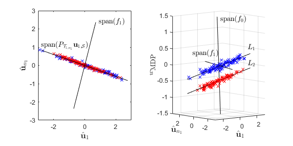
Figure 6: $2$-dimensional projections onto $\mathcal{T}_{1,n_{1}}={\rm span}(\hat{\mathbf{u}}_{1},\hat{\mathbf{u}}_{n_{1}})$ and $3$-dimensional projections onto $\mathcal{S}=\mathcal{T}_{1,n_{1}}\oplus{\rm span}(w_{\textup{MDP}})$ of independent test data $\mathcal{Y}$ (class 1: blue crosses, class 2: red crosses) under the model in Example 3. The left panel shows that projections of $\mathcal{Y}$ onto $\mathcal{T}_{1,n_{1}}$ are concentrated along the direction of ${\rm span}(P_{\mathcal{T}_{1,n_{1}}}\mathbf{u}_{1,\mathcal{S}})$. However, $f_{1}\in\mathcal{T}_{1,n_{1}}$, which is orthogonal to $\mathbf{u}_{1,\mathcal{S}}$, is not a meaningful second data piling direction since projections of $\mathcal{Y}_{1}$ and $\mathcal{Y}_{2}$ onto $f_{1}$ will be piled on a same location. The right panel shows that projections of $\mathcal{Y}$ onto $\mathcal{S}$ are concentrated along parallel lines $L_{1}$ and $L_{2}$, which are also parallel to $\mathbf{u}_{1,\mathcal{S}}$ (See Proposition 2 and Theorem 6). Then $f_{0}\in\mathcal{S}$, which is orthogonal to both of $\mathbf{u}_{1,\mathcal{S}}$ and $f_{1}$, gives a meaningful distance between the two piles of independent test data $\mathcal{Y}$.

Figure 7: Projections of $v_{-\tau_{1}^{2}}$ and $v_{-\tau_{2}^{2}}$ onto ${\rm span}(f_{0})\oplus{\rm span}(f_{1})$. Note that any direction $w\in{\rm span}(f_{0})\oplus{\rm span}(f_{1})$ yields second data piling. Both of $v_{-\tau_{1}^{2}}$ and $v_{-\tau_{2}^{2}}$ are not the same directions with $f_{0}$, which is a second maximal data piling direction.

Proposition 19

Suppose Assumptions 1—5 hold and assume $\beta_{1}=\beta_{2}=1$, $\tau_{1}^{2}>\tau_{2}^{2}$ and $m_{1}=m_{2}=m=1$. Then,

• $$\frac{1}{\sqrt{p}}f_{1}^{\top}(Y-\bar{X})\xrightarrow{P}\begin{cases}0,&\pi(Y)=1,\\ 0,&\pi(Y)=2\end{cases}$$

  as $p\to\infty$.

• $$\frac{1}{\sqrt{p}}f_{0}^{\top}(Y-\bar{X})\xrightarrow{P}\begin{cases}\upsilon_{0}(\eta_{2}(1-\cos^{2}\varphi)\delta^{2}-(\tau_{1}^{2}-\tau_{2}^{2})/n),&\pi(Y)=1,\\ \upsilon_{0}(-\eta_{1}(1-\cos^{2}\varphi)\delta^{2}-(\tau_{1}^{2}-\tau_{2}^{2})/n),&\pi(Y)=2\end{cases}$$

  as $p\to\infty$ where $\upsilon_{0}$ is a strictly positive random variable depending on the true principal component scores of $\mathcal{X}$.

• For $k=1,2$, $\upsilon_{0}>\gamma_{k}$ with probability $1$ where $\gamma_{k}$ is defined in Proposition 16.

See (82) in Appendix D for the definition of $\upsilon_{0}$.

In fact, $f_{0}$ gives the largest distance between the two piles of independent test data. To see this, we characterize the collection of all second data piling directions using $f_{0}$, $f_{1}$ and $\left\{\hat{\mathbf{u}}_{i}\right\}_{i\in\left\{1,\ldots,n-2\right\}\setminus\mathcal{D}}$. In particular, Proposition 20 states that any given $\left\{w\right\}\in\mathcal{A}$ is asymptotically close to a sequence $\left\{v\right\}$, where $v$ is in a subspace spanned by $f_{0}$, $f_{1}$ and $\left\{\hat{\mathbf{u}}_{i}\right\}_{i\in\left\{1,\ldots,n-2\right\}\setminus\mathcal{D}}$. Since $f_{0}$ gives meaningful asymptotic distance between the two piles of independent test data while $f_{1}$ and $\left\{\hat{\mathbf{u}}_{i}\right\}_{i\in\left\{1,\ldots,n-2\right\}\setminus\mathcal{D}}$ do not, $f_{0}$ naturally becomes a second maximal data piling direction.

Proposition 20

Suppose Assumptions 1—5 hold and assume $\beta_{1}=\beta_{2}=1$, $\tau_{1}^{2}>\tau_{2}^{2}$ and $m_{1}=m_{2}=m=1$. Then,

• For any given $\left\{w\right\}\in\mathcal{A}$, there exists a sequence $\left\{v\right\}\in\mathcal{B}$ such that $\|w-v\|\xrightarrow{P}0$ as $p\to\infty$, where $\mathcal{B}=\left\{\left\{v\right\}\in\mathfrak{W}_{X}:v\in{\rm span}(f_{0})\oplus{\rm span}(f_{1})\oplus{\rm span}(\left\{\hat{\mathbf{u}}_{i}\right\}_{i\in\left\{1,\ldots,n-2\right\}\setminus\mathcal{D}})\right\}$.

• For any $\left\{w\right\}\in\mathcal{A}$ such that $D(w)$ exists, $\left\{w\right\}$ is a sequence of second maximal data piling directions if and only if $\|w-f_{0}\|\xrightarrow{P}0$ as $p\to\infty$.

Note that each of $\left\{v_{\hat{\alpha}_{1}}\right\}$ and $\left\{v_{\hat{\alpha}_{2}}\right\}$ is asymptotically close to a sequence $\left\{w\right\}$ respectively, where $w\in{\rm span}(f_{0})\oplus{\rm span}(f_{1})$. It can be seen that neither $v_{\hat{\alpha}_{1}}$ nor $v_{\hat{\alpha}_{2}}$ is a second maximal data piling direction since these classifiers are affected by the noisy direction $f_{1}$ (See Figure 7).

5.2 One-component Covariance Model with $m=2$

Next, assume $m=2$ (that is, $\mathbf{u}_{(1),1}\neq\mathbf{u}_{(2),1}$). Note that $\mathcal{S}={\rm span}(\hat{\mathbf{u}}_{1},\hat{\mathbf{u}}_{2},\hat{\mathbf{u}}_{n_{1}},w_{\textup{MDP}})$ and $\dim{\mathcal{S}}-m=2$. For this case, a direction $w\in\mathcal{S}$ yields second data piling if $w$ is asymptotically orthogonal to the $2$-dimensional common leading eigenspace $P_{\mathcal{S}}\mathcal{U}={\rm span}(\mathbf{u}_{(1),1,\mathcal{S}},\mathbf{u}_{(2),1,\mathcal{S}})$.

As seen in Example 4, either $\hat{\mathbf{u}}_{2}$ or $\hat{\mathbf{u}}_{n_{1}}$ is a noisy direction which explains the deterministic simplex of data from the first class, not the variability within the common leading eigenspace $\mathcal{U}$. Hence, the projected ridged linear discriminant vector,

$$v_{\alpha}\varpropto\sum_{i\in\left\{1,2,n_{1}\right\}}\frac{\alpha_{p}}{\hat{\lambda}_{i}+\alpha_{p}}\hat{\mathbf{u}}_{i}\hat{\mathbf{u}}_{i}^{\top}\mathbf{d}+\hat{\mathbf{U}}_{2}\hat{\mathbf{U}}_{2}^{\top}\mathbf{d},$$

is affected by the noisy direction (either $\hat{\mathbf{u}}_{2}$ or $\hat{\mathbf{u}}_{n_{1}}$). For any given training data $\mathcal{X}$, we define the ‘conditioned’ projected ridged linear discriminant vector $v_{\alpha}^{c}$ as

$$v_{\alpha}^{c}\varpropto v_{\alpha}-\sum_{i\in\mathcal{D}\setminus\mathcal{D}^{\prime}}\frac{\alpha_{p}}{\hat{\lambda}_{i}+\alpha_{p}}\hat{\mathbf{u}}_{i}\hat{\mathbf{u}}_{i}^{\top}\mathbf{d}=\sum_{i\in\mathcal{D}^{\prime}}\frac{\alpha_{p}}{\hat{\lambda}_{i}+\alpha_{p}}\hat{\mathbf{u}}_{i}\hat{\mathbf{u}}_{i}^{\top}\mathbf{d}+\hat{\mathbf{U}}_{2}\hat{\mathbf{U}}_{2}^{\top}\mathbf{d}$$ (19)

satisfying $\|v_{\alpha}^{c}\|=1$ to remove all the noisy terms in the ridged linear discriminant vector $w_{\alpha}$. Recall that in this case $\mathcal{D}^{\prime}$ is either $\left\{1,2\right\}$ or $\left\{1,n_{1}\right\}$ depending on the true leading principal component scores. Proposition 21 implies that $v_{\hat{\alpha}_{k}}^{c}$ is asymptotically orthogonal to $\mathbf{u}_{(k),1}$, which is the leading eigenvector of the $k$th class.

Proposition 21

Suppose Assumptions 1—5 hold and assume $\beta_{1}=\beta_{2}=1$, $\tau_{1}^{2}>\tau_{2}^{2}$, $m_{1}=m_{2}=1$ and $m=2$. For any given training data $\mathcal{X}$ and $\hat{\alpha}_{k}$ chosen as an HDLSS-consistent estimator of $-\tau_{k}^{2}$, $\mbox{Angle}{(v_{\hat{\alpha}_{k}}^{c},\mathbf{u}_{(k),i,\mathcal{S}})}\xrightarrow{P}\pi/2$ as $p\to\infty$ for $k=1,2$.

However, Theorem 22 shows that there is no ridge parameter $\alpha\in\mathbb{R}$ which induces $v_{\alpha}^{c}$ to be asymptotically orthogonal to both of $\mathbf{u}_{(1),1}$ and $\mathbf{u}_{(2),1}$.

Theorem 22

Suppose Assumptions 1—5 hold and assume $\beta_{1}=\beta_{2}=1$, $\tau_{1}^{2}>\tau_{2}^{2}$, $m_{1}=m_{2}=1$ and $m=2$. For any given training data $\mathcal{X}$, $\left\{v_{\alpha}^{c}\right\}\notin\mathcal{A}$ for any ridge parameter $\alpha\in\mathbb{R}$.

Hence, for any given training data $\mathcal{X}$, $v_{\alpha}^{c}$ does not yield second data piling for all $\alpha\in\mathbb{R}$. It implies that $v_{\alpha}$ can also not be a second data piling direction for all $\alpha\in\mathbb{R}$.

In general, we can show that $v_{\hat{\alpha}_{k}}^{c}$ is asymptotically orthogonal to $\mathcal{U}_{(k)}$, which is the leading eigenspace of the $k$th class for $k=1,2$. However, as shown in the above, this fact does not imply that $v_{\alpha}^{c}$ yields second data piling for some $\alpha\in\mathbb{R}$. Nonetheless, if the leading eigenspace of the one class includes that of the other class (as in Section 5.1), then $v_{\alpha}^{c}$ can yield second data piling with a negative ridge parameter. See Appendix A for more details.

5.3 Second Maximal Data Piling Direction for Generalized Heterogeneous Spiked Covariance Model

So far, we have seen that $v_{\alpha}$ may not be a second maximal data piling direction, and may not even yield second data piling for any ridge parameter $\alpha\in\mathbb{R}$. In this subsection, we introduce the idea of characterizing the collection of sequences of second data piling directions $\mathcal{A}$ for general $m_{1}\geq 1$ and $m_{2}\geq 1$. For any given training data $\mathcal{X}$, note that $\hat{\mathbf{u}}_{i}$ for $i\in\left\{1,\ldots,n-2\right\}\setminus\mathcal{D}^{\prime}$ is asymptotically orthogonal to ${\rm span}(\mathbf{U}_{1,\mathcal{S}})$. Next, as in Section 5.1, we can find $(m_{1}+m_{2}-m)$-dimensional subspace $\mathcal{T}_{p}\leq{\rm span}(\left\{\hat{\mathbf{u}}_{i}\right\}_{i\in\mathcal{D}^{\prime}})$ such that any direction $w\in\mathcal{T}_{p}$ is asymptotically orthogonal to $m$-dimensional subspace ${\rm span}(\mathbf{U}_{1,\mathcal{S}})$. Note that $w\in\mathcal{T}_{p}$ is also orthogonal to $w_{\textup{MDP}}$. We define a collection of sequences

$$\mathcal{T}=\left\{\left\{w\right\}\in\mathfrak{W}_{X}:w\in\mathcal{T}_{p}\oplus{\rm span}(\left\{\hat{\mathbf{u}}_{i}\right\}_{i\in\mathcal{D}\setminus\mathcal{D}^{\prime}})\leq\mathcal{S}\text{ for all }p\right\}.$$

Lastly, we can find $\left\{f_{0}\right\}$ such that $f_{0}\in\mathcal{S}^{\prime}$, and $f_{0}$ is not only orthogonal to $\mathcal{T}_{p}$ and but also asymptotically orthogonal to ${\rm span}(\mathbf{U}_{1,\mathcal{S}})$. For detailed construction of $\mathcal{T}_{p}$ and $f_{0}$, see Appendix D.12.

Theorem 23

Suppose Assumptions 1—5 hold and assume $\beta_{1}=\beta_{2}=1$, $\tau_{1}^{2}>\tau_{2}^{2}$. Then,

• For any $\left\{w\right\}\in\mathcal{T}$,

  $$\frac{1}{\sqrt{p}}w^{\top}(Y-\bar{X})\xrightarrow{P}\begin{cases}0,&\pi(Y)=1,\\ 0,&\pi(Y)=2\end{cases}$$

  as $p\to\infty$.

• $$\frac{1}{\sqrt{p}}f_{0}^{\top}(Y-\bar{X})\xrightarrow{P}\begin{cases}\upsilon_{0}(\eta_{2}(1-\cos^{2}\varphi)\delta^{2}-(\tau_{1}^{2}-\tau_{2}^{2})/n)&\pi(Y)=1,\\ \upsilon_{0}(-\eta_{1}(1-\cos^{2}\varphi)\delta^{2}-(\tau_{1}^{2}-\tau_{2}^{2})/n)&\pi(Y)=2\end{cases}$$

  as $p\to\infty$ with a strictly positive random variable $\upsilon_{0}$.

See (86) for the definition of $\upsilon_{0}$. Theorem 23 shows that $\left\{f_{0}\right\}$ gives a meaningful distance between the two piles of independent test data while $\left\{w\right\}\in\mathcal{T}$ does not. It naturally implies that $f_{0}$ is a second maximal data piling direction.

Theorem 24

Suppose Assumptions 1—5 hold and assume $\beta_{1}=\beta_{2}=1$, $\tau_{1}^{2}>\tau_{2}^{2}$. Then,

• For any given $\left\{w\right\}\in\mathcal{A}$, there exists a sequence $\left\{v\right\}\in\mathcal{B}$ such that $\|w-v\|\xrightarrow{P}0$ as $p\to\infty$, where $\mathcal{B}=\left\{\left\{v\right\}\in\mathfrak{W}_{X}:v\in{\rm span}(f_{0})\oplus\mathcal{T}_{p}\oplus{\rm span}(\left\{\hat{\mathbf{u}}_{i}\right\}_{i\in\left\{1,\ldots,n-2\right\}\setminus\mathcal{D}^{\prime}})\right\}$.

• For any $\left\{w\right\}\in\mathcal{A}$ such that $D(w)$ exists, $\left\{w\right\}$ is a sequence of second maximal data piling directions if and only if $\|w-f_{0}\|\xrightarrow{P}0$ as $p\to\infty$.

It is important to note that a second maximal data piling direction is a direction $w\in\mathcal{S}^{\prime}$ which is asymptotically orthogonal to both of ${\rm span}(\mathbf{U}_{1,\mathcal{S}})$ and $\mathcal{T}_{p}$. The dimension of the orthogonal complement of ${\rm span}(\mathbf{U}_{1,\mathcal{S}})$ within $\mathcal{S}$, say $\mathbf{U}_{1,\mathcal{S}}^{\perp}$, is in general greater than one. A second maximal data piling direction lies in $\mathbf{U}_{1,\mathcal{S}}^{\perp}$, but is also orthogonal to $\mathcal{T}_{p}$ that is orthogonal to $w_{\textup{MDP}}$. That is, second maximal data piling direction can be achieved when $w_{\textup{MDP}}$ is projected onto the orthogonal complement of ${\rm span}(\mathbf{U}_{1,\mathcal{S}})$. This observation gives a unified view on the theoretical second maximal data piling direction and the estimates of such directions ($w_{\textup{MDP}},v_{\hat{\alpha}}$ in Section 4): These directions are the projection of $w_{\textup{MDP}}$ onto the orthogonal complement of ${\rm span}(\mathbf{U}_{1,\mathcal{S}})$ (or its estimate).

5.4 Data-splitting Approach for Second Maximal Data Piling Direction

In this subsection, we propose a data-splitting approach to estimate a second maximal data piling direction, which can be applied to all cases we have discussed. Let $\mathbf{V}=[\hat{\mathbf{u}}_{1},\ldots,\hat{\mathbf{u}}_{n-2},w_{\textup{MDP}}]$, which collects an orthonormal basis of the sample space $\mathcal{S}_{X}$. Also, in this subsection, we assume that an independent test dataset $\mathcal{Y}$ is available to us (It is possible by splitting the original training dataset $\mathcal{X}$ into the new training dataset $\mathcal{X}$ and the test dataset $\mathcal{Y}$). Denote the horizontally concatenated data matrix of the given independent test dataset $\mathcal{Y}$ by

$$\mathbf{Y}=[Y_{11},\ldots,Y_{1n_{1}^{*}},Y_{21},\ldots,Y_{2n_{2}^{*}}].$$

The $p\times n^{*}$ data matrix $\mathbf{Y}$ consists of the $n^{*}:=n_{1}^{*}+n_{2}^{*}$ observations independent to $\mathcal{X}$ and arranged so that $\pi(Y_{kj})=k$ for any $k,j$. We assume that $n_{k}^{*}$ is fixed and $n_{k}^{*}>m_{k}$ for $k=1,2$. Write class-wise sample mean vectors $\bar{Y}_{k}=n_{k}^{*-1}\sum_{j=1}^{n_{k}^{*}}Y_{kj}$. We define the within-scatter matrix of $\mathcal{Y}$ as

$$\mathbf{S}_{W}^{*}=\sum_{k=1}^{2}(\mathbf{Y}_{k}-\bar{\mathbf{Y}}_{k})(\mathbf{Y}_{k}-\bar{\mathbf{Y}}_{k})^{\top}=(\mathbf{Y}-\bar{\mathbf{Y}})(\mathbf{Y}-\bar{\mathbf{Y}})^{\top},$$

where $\bar{\mathbf{Y}}_{k}=\bar{Y}_{k}\mathbf{1}_{n_{k}^{*}}^{\top}$ for $k=1,2$ and $\bar{\mathbf{Y}}=[\bar{\mathbf{Y}}_{1}~{}\bar{\mathbf{Y}}_{2}]$.

We will find a sequence of directions $\left\{w\right\}\in\mathfrak{W}_{X}$ which yields second data piling for given independent test dataset $\mathcal{Y}$. The condition that $p^{-1/2}w^{\top}(Y-Y^{\prime})\xrightarrow{P}0$ as $p\to\infty$ for any $Y,Y^{\prime}\in\mathcal{Y}$ with $\pi(Y)=\pi(Y^{\prime})$ is equivalent to the condition that

$$\frac{1}{p}w^{\top}\mathbf{S}_{W}^{*}w\xrightarrow{P}0$$

as $p\to\infty$. Thus, we define the collection of sequences of second data piling directions for $\mathcal{Y}$ as

$$\bar{\mathcal{A}}=\left\{\left\{w\right\}\in\mathfrak{W}_{X}:\frac{1}{p}w^{\top}\mathbf{S}_{W}^{*}w\xrightarrow{P}0\text{ as }p\to\infty\right\}.$$

For any $\left\{w\right\}\in\mathfrak{W}_{X}$, we can write $w=\mathbf{V}\mathbf{a}$ for some $\mathbf{a}=(a_{1},\ldots,a_{n-2},a_{\textup{MDP}})^{\top}\in\mathbb{R}^{n-1}$. Without loss of generality, we assume $a_{\textup{MDP}}\geq 0$ for all $p$. For $\left\{w\right\}\in\bar{\mathcal{A}}$, we can write

$$\frac{1}{p}w^{\top}\mathbf{S}_{W}^{*}w=\frac{1}{p}\mathbf{a}^{\top}\mathbf{V}^{\top}\mathbf{S}_{W}^{*}\mathbf{V}\mathbf{a}=\mathbf{a}^{\top}\left(\frac{1}{p}\mathbf{V}^{\top}\mathbf{S}_{W}^{*}\mathbf{V}\right)\mathbf{a}.$$ (20)

Note that the $(n-1)\times(n-1)$ matrix $p^{-1}\mathbf{V}^{\top}\mathbf{S}_{W}^{*}\mathbf{V}$ can be understood as the scatter of the independent test data $\mathcal{Y}$ projected onto the sample space $\mathcal{S}_{X}$. Theorem 25 shows that independent test data $\mathcal{Y}$ are asymptotically supported on a $m$-dimensional subspace in $\mathcal{S}_{X}$.

Theorem 25

$p^{-1}\mathbf{V}^{\top}\mathbf{S}_{W}^{*}\mathbf{V}$ converges to a rank $m$ matrix in probability as $p\to\infty$.

We write an eigen-decomposition of $p^{-1}\mathbf{V}^{\top}\mathbf{S}_{W}^{*}\mathbf{V}=\hat{\mathbf{Q}}\mathbf{H}\hat{\mathbf{Q}}^{\top}$, where $\mathbf{H}=\mbox{Diag}{(h_{1},\ldots,h_{n-1})}$ arranged in descending order, and $\hat{\mathbf{Q}}=[\hat{\mathbf{Q}}_{1}~{}\hat{\mathbf{Q}}_{2}]$ with $\hat{\mathbf{Q}}_{1}=[\hat{\mathbf{q}}_{1},\ldots,\hat{\mathbf{q}}_{m}]$ and $\hat{\mathbf{Q}}_{2}=[\hat{\mathbf{q}}_{m+1},\ldots,\hat{\mathbf{q}}_{n-1}]$. Meanwhile, $\mathbf{a}$ can be written as $\mathbf{a}=\hat{\mathbf{Q}}\mbox{\boldmath{$\iota$}}=\sum_{i=1}^{n-1}\iota_{i}\hat{\mathbf{q}}_{i}$ for some sequence of $\mbox{\boldmath{$\iota$}}=(\iota_{1},\ldots,\iota_{n-1})^{\top}$. Since

$$\frac{1}{p}w^{\top}\mathbf{S}_{W}^{*}w=\mathbf{a}^{\top}\left(\frac{1}{p}\mathbf{V}^{\top}\mathbf{S}_{W}^{*}\mathbf{V}\right)\mathbf{a}=\sum_{i=1}^{n-1}h_{i}\iota_{i}^{2}=\sum_{i=1}^{m}h_{i}\iota_{i}^{2}+o_{p}(1)$$

by Theorem 25 and (20), $\left\{w\right\}\in\bar{\mathcal{A}}$ if and only if $\iota_{1},\ldots,\iota_{m}\xrightarrow{P}0$ as $p\to\infty$. In other words, for any given $\left\{w\right\}\in\bar{\mathcal{A}}$, there exists a sequence of directions $\left\{v\right\}$ such that $v\in{\rm span}(\mathbf{V}\hat{\mathbf{Q}}_{2})$ for all $p$ and $\|w-v\|\xrightarrow{P}0$ as $p\to\infty$. This fact plays a crucial role in our next observation: $\left\{w\right\}\in\bar{\mathcal{A}}$ is indeed asymptotically orthogonal to the common leading eigenspace $\mathcal{U}$.

Theorem 26

Suppose Assumptions 1—5 hold. For any given $\left\{w\right\}\in\bar{\mathcal{A}}$, $w^{\top}\mathbf{u}_{j}\xrightarrow{P}0$ for $1\leq j\leq m$.

Furthermore, $\left\{w\right\}\in\bar{\mathcal{A}}$ can also achieve perfect classification of any independent observation $Y$, which is independent to both of $\mathcal{X}$ and $\mathcal{Y}$. Theorem 27 confirms that we can achieve perfect classification if we choose $\mathbf{a}$ so that for $w=\mathbf{V}\mathbf{a}$, $\left\{w\right\}\in\bar{\mathcal{A}}$ and $\lim_{p\to\infty}a_{\textup{MDP}}>0$. Note that $\mathbf{a}$ can be viewed as a function of training data $\mathcal{X}$ (that is, $\mathbf{a}=\mathbf{a}(\mathcal{X})$).

Theorem 27

Suppose Assumptions 1—5 hold. For any given $\left\{w\right\}\in\bar{\mathcal{A}}$, write

$$w=\mathbf{V}\mathbf{a}=\sum_{k=1}^{n-2}a_{k}\hat{\mathbf{u}}_{k}+a_{\textup{MDP}}w_{\textup{MDP}}$$

with $\mathbf{a}=(a_{1},\ldots,a_{n-2},a_{\textup{MDP}})^{\top}$ and assume $a_{\textup{MDP}}\xrightarrow{P}\psi_{\textup{MDP}}$ as $p\to\infty$. Then for any independent observation $Y$, which is independent to both of $\mathcal{X}$ and $\mathcal{Y}$,

$$\frac{1}{\sqrt{p}}w^{\top}(Y-\bar{X})\xrightarrow{P}\begin{cases}\frac{\psi_{\textup{MDP}}}{\kappa}(\eta_{2}(1-\cos^{2}\varphi)\delta^{2}-(\tau_{1}^{2}-\tau_{2}^{2})/n),&\pi(Y)=1,\\ \frac{\psi_{\textup{MDP}}}{\kappa}(-\eta_{1}(1-\cos^{2}\varphi)\delta^{2}-(\tau_{1}^{2}-\tau_{2}^{2})/n),&\pi(Y)=2,\end{cases}$$

as $p\to\infty$, where $\kappa$ is the probability limit of $\kappa_{\textup{MDP}}$ defined in (2).

Theorem 27 also shows that an asymptotic distance between the two piles of independent test data, which are independent to both of $\mathcal{X}$ and $\mathcal{Y}$, can be maximized if $\left\{w\right\}\in\bar{\mathcal{A}}$ with $w=\mathbf{V}\mathbf{a}$ has a maximal limit of $a_{\textup{MDP}}$. Theorem 28 confirms that a projection of $w_{\textup{MDP}}$ onto ${\rm span}(\mathbf{V}\hat{\mathbf{Q}}_{2})$ is an estimate of a second maximal data piling direction. Recall that $\mathbf{V}\hat{\mathbf{Q}}_{2}$ is obtainable by using $\mathcal{X}$ and $\mathcal{Y}$, and the dimension of ${\rm span}(\mathbf{V}\hat{\mathbf{Q}}_{2})$ is $n-m-1$. It implies that a second maximal data piling direction can be obtained by projecting $w_{\textup{MDP}}$ onto the nullspace of the common leading eigenspace $\mathcal{U}$.

Theorem 28

Suppose Assumptions 1—5 hold. Write $\mathbf{e}_{\textup{MDP}}=(\mathbf{0}_{n-2}^{\top},~{}1)^{\top}$ so that $w_{\textup{MDP}}=\mathbf{V}\mathbf{e}_{\textup{MDP}}$. Also, let $\left\{w_{\textup{SMDP}}\right\}$ be a sequence of directions such that $w_{\textup{SMDP}}=\mathbf{V}\mathbf{a}_{\textup{SMDP}}$ where

$$\mathbf{a}_{\textup{SMDP}}=\frac{P_{{\rm span}(\hat{\mathbf{Q}}_{2})}{\mathbf{e}_{\textup{MDP}}}}{\|P_{{\rm span}(\hat{\mathbf{Q}}_{2})}{\mathbf{e}_{\textup{MDP}}}\|}=\frac{\hat{\mathbf{Q}}_{2}\hat{\mathbf{Q}}_{2}^{\top}\mathbf{e}_{\textup{MDP}}}{\|\hat{\mathbf{Q}}_{2}\hat{\mathbf{Q}}_{2}^{\top}\mathbf{e}_{\textup{MDP}}\|}\in\mathbb{R}^{n-1}.$$

Then $\left\{w\right\}\in\bar{\mathcal{A}}$ is a sequence of second maximal data piling directions if and only if $\|w-w_{\textup{SMDP}}\|\xrightarrow{P}0$ as $p\to\infty$.

5.5 Computational Algorithm

We have shown that a second maximal data piling direction in the sample space $\mathcal{S}_{X}$ can be obtained with a help of independent test data. As such, we randomly split $\mathcal{X}_{k}$, which is the original training dataset of the $k$th class, into training dataset $\mathcal{X}_{k,tr}$ and test dataset $\mathcal{X}_{k,te}$ so that the sample size of test data of $k$th class $n_{k,te}$ is larger than $m_{k}$ for $k=1,2$. Then we can find a second maximal data piling direction in the sample space of $\mathcal{X}_{tr}=\mathcal{X}_{1,tr}\cup\mathcal{X}_{2,tr}$ with a help of $\mathcal{X}_{te}=\mathcal{X}_{1,te}\cup\mathcal{X}_{2,te}$.

The fact that the sample size of HDLSS data is very small implies that classification using one data split may be unreliable (albeit theoretically true). In order to resolve this concern, we repeat the above procedure several times and set a final estimate of a second maximal data piling direction as the average of estimates of a second maximal data piling direction obtained from each repetition. A detailed algorithm is given in Algorithm 1. In practice, we should estimate $m_{1}$, $m_{2}$ and $m$, which are the true numbers of leading eigenvalues of $\mbox{\boldmath{$\Sigma$}}_{(1)}$, $\mbox{\boldmath{$\Sigma$}}_{(2)}$ and $\mbox{\boldmath{$\Sigma$}}_{(0)}=\pi_{1}\mbox{\boldmath{$\Sigma$}}_{(1)}+\pi_{2}\mbox{\boldmath{$\Sigma$}}_{(2)}$ for Algorithm 1. Estimating those numbers is feasible by Kritchman and Nadler (2008), Leek (2010), Passemier and Yao (2014) and Jung et al. (2018).

Algorithm 1 Second Maximal Data Piling (SMDP) algorithm (Type I)

1:Original training data matrix of the $k$th class $\mathbf{X}_{k}$ for $k=1,2$.

2:The number of repetitions $K$, estimated $m_{1}$, $m_{2}$ and $m$

3:for $j=1,\ldots,K$ do

4:     Randomly split $\mathbf{X}_{k}$ into $\begin{cases}\mathbf{X}_{k,tr}=[X_{k,1},\ldots,X_{k,n_{k,tr}}]\\ \mathbf{X}_{k,te}=[X_{k,1}^{*},\ldots,X_{k,n_{k,te}}^{*}]\end{cases}$ so that $n_{k,te}>m_{k}$ ($k=1,2$)

5:     Set $n_{tr}=n_{1,tr}+n_{2,tr}$, $\bar{X}_{k,tr}=n_{k}^{-1}\mathbf{X}_{k,tr}\mathbf{1}_{n_{k,tr}}$ and $\bar{\mathbf{X}}_{k,tr}=\bar{X}_{k,tr}\mathbf{1}_{n_{k,tr}}^{\top}$ ($k=1,2$)

6:     Set $\mathbf{S}_{tr}=\sum_{k=1}^{2}(\mathbf{X}_{k,tr}-\bar{\mathbf{X}}_{k,tr})(\mathbf{X}_{k,tr}-\bar{\mathbf{X}}_{k,tr})^{\top}$ and $\mathbf{d}_{tr}=\bar{X}_{1,tr}-\bar{X}_{2,tr}$

7:     Write an eigen-decomposition of $\mathbf{S}_{tr}$ by $\mathbf{S}_{tr}=\hat{\mathbf{U}}\hat{}\mbox{\boldmath{$\Lambda$}}\hat{\mathbf{U}}^{\top}=\hat{\mathbf{U}}_{1}\hat{}\mbox{\boldmath{$\Lambda$}}_{1}\hat{\mathbf{U}}_{1}^{\top}$ where $\hat{}\mbox{\boldmath{$\Lambda$}}=\mbox{Diag}{(\hat{\lambda}_{1},\ldots,\hat{\lambda}_{n_{tr}-2},0,\ldots,0)}$ arranged in descending order, and $\hat{\mathbf{U}}=[\hat{\mathbf{U}}_{1}~{}\hat{\mathbf{U}}_{2}]$ with $\hat{\mathbf{U}}_{1}=[\hat{\mathbf{u}}_{1},\ldots,\hat{\mathbf{u}}_{n_{tr}-2}]$, $\hat{\mathbf{U}}_{2}=[\hat{\mathbf{u}}_{n_{tr}-1},\ldots,\hat{\mathbf{u}}_{p}]$

8:     Set $w_{\textup{MDP}}=\|\hat{\mathbf{U}}_{2}\hat{\mathbf{U}}_{2}^{\top}\mathbf{d}_{tr}\|^{-1}\hat{\mathbf{U}}_{2}\hat{\mathbf{U}}_{2}^{\top}\mathbf{d}_{tr}$ and $\kappa_{\textup{MDP}}=p^{-1/2}\|\hat{\mathbf{U}}_{2}\hat{\mathbf{U}}_{2}^{\top}\mathbf{d}_{tr}\|$

9:     Set $\mathbf{V}=[\hat{\mathbf{u}}_{1},\ldots,\hat{\mathbf{u}}_{n_{tr}-2},w_{\textup{MDP}}]$

10:     Set $\bar{X}_{k,te}=n_{k,te}^{-1}\mathbf{X}_{k,te}\mathbf{1}_{n_{k,te}}$ and $\bar{\mathbf{X}}_{k,te}=\bar{X}_{k,te}\mathbf{1}_{n_{k,te}}^{\top}$ ($k=1,2$)

11:     Set $\mathbf{S}_{te}=\sum_{k=1}^{2}(\mathbf{X}_{k,te}-\bar{\mathbf{X}}_{k,te})(\mathbf{X}_{k,te}-\bar{\mathbf{X}}_{k,te})^{\top}$

12:     Write an eigen-decomposition of $p^{-1}\mathbf{V}^{\top}\mathbf{S}_{te}\mathbf{V}$ by $p^{-1}\mathbf{V}^{\top}\mathbf{S}_{te}\mathbf{V}=\hat{\mathbf{Q}}\mathbf{H}\hat{\mathbf{Q}}^{\top}$ where $\mathbf{H}=\mbox{Diag}{(h_{1},\ldots,h_{n_{tr}-1})}$ arranged in descending order, and $\hat{\mathbf{Q}}=[\hat{\mathbf{Q}}_{1}~{}\hat{\mathbf{Q}}_{2}]$ with $\hat{\mathbf{Q}}_{1}=[\hat{\mathbf{q}}_{1},\ldots,\hat{\mathbf{q}}_{m}]$ and $\hat{\mathbf{Q}}_{2}=[\hat{\mathbf{q}}_{m+1},\ldots,\hat{\mathbf{q}}_{n_{tr}-1}]$

13:     Set $\mathbf{a}_{j,\textup{SMDP}}=\|\hat{\mathbf{Q}}_{2}\hat{\mathbf{Q}}_{2}^{\top}\mathbf{e}_{\textup{MDP}}\|^{-1}\hat{\mathbf{Q}}_{2}\hat{\mathbf{Q}}_{2}^{\top}\mathbf{e}_{\textup{MDP}}$ where $\mathbf{e}_{\textup{MDP}}=(\mathbf{0}_{n-2}^{\top},1)^{\top}$

14:     Set $w_{j,\textup{SMDP}}=\mathbf{V}\mathbf{a}_{j,\textup{SMDP}}$

15:     Set $\bar{X}_{j,\textup{SMDP}}=n_{tr}^{-1}(n_{1,tr}\bar{X}_{1,tr}+n_{2,tr}\bar{X}_{2,tr})$

16:     Set $\hat{\alpha}_{k}=-p^{-1}\sum_{k=m_{k}+1}^{n_{k,tr}-1}\hat{\lambda}_{(k),l}$ where $\hat{\lambda}_{(k),l}$ is $l$th largest eigenvalue of

$$\mathbf{S}_{k,tr}=(\mathbf{X}_{k,tr}-\bar{\mathbf{X}}_{k,tr})(\mathbf{X}_{k,tr}-\bar{\mathbf{X}}_{k,tr})^{\top}$$

17:     Set $g_{j,\textup{SMDP}}=(n_{tr}\kappa_{\textup{MDP}})^{-1}(\mathbf{e}_{\textup{MDP}}^{\top}\mathbf{a}_{j,\textup{SMDP}})(\hat{\alpha}_{1}-\hat{\alpha}_{2})$

18:end for

19:Set $w_{\textup{SMDP}}=K^{-1}\sum_{j=1}^{K}w_{j,\textup{SMDP}}$

20:Set $\bar{X}_{\textup{SMDP}}=K^{-1}\sum_{j=1}^{K}w_{j,\textup{SMDP}}^{\top}\bar{X}_{j,\textup{SMDP}}$

21:Set $g_{\textup{SMDP}}=K^{-1}\sum_{j=1}^{K}g_{j,\textup{SMDP}}$

22:Use the following classification rule:

$$\phi_{\textup{SMDP-I}}(Y;\mathcal{X})=\begin{cases}1,&p^{-1/2}(w_{\textup{SMDP}}^{\top}Y-\bar{X}_{\textup{SMDP}})-g_{\textup{SMDP}}\geq 0,\\ 2,&p^{-1/2}(w_{\textup{SMDP}}^{\top}Y-\bar{X}_{\textup{SMDP}})-g_{\textup{SMDP}}<0.\end{cases}$$ (21)

Algorithm 2 Second Maximal Data Piling (SMDP) algorithm (Type II)

1:Original training data matrix of the $k$th class $\mathbf{X}_{k}$ for $k=1,2$.

2:The number of repetitions $K$, estimated $m$

3:for $j=1,\ldots,K$ do

4:     Randomly split $\mathbf{X}_{k}$ into $\begin{cases}\mathbf{X}_{k,tr}=[X_{k,1},\ldots,X_{k,n_{k,tr}}]\\ \mathbf{X}_{k,te}=[X_{k,1}^{*},\ldots,X_{k,n_{k,te}}^{*}]\end{cases}$ so that $n_{k,te}>m_{k}$ ($k=1,2$)

5:     Set $n_{tr}=n_{1,tr}+n_{2,tr}$, $\bar{X}_{k,tr}=n_{k}^{-1}\mathbf{X}_{k,tr}\mathbf{1}_{n_{k,tr}}$ and $\bar{\mathbf{X}}_{k,tr}=\bar{X}_{k,tr}\mathbf{1}_{n_{k,tr}}^{\top}$ ($k=1,2$)

6:     Set $\mathbf{S}_{tr}=\sum_{k=1}^{2}(\mathbf{X}_{k,tr}-\bar{\mathbf{X}}_{k,tr})(\mathbf{X}_{k,tr}-\bar{\mathbf{X}}_{k,tr})^{\top}$ and $\mathbf{d}_{tr}=\bar{X}_{1,tr}-\bar{X}_{2,tr}$

7:     Write an eigen-decomposition of $\mathbf{S}_{tr}$ by $\mathbf{S}_{tr}=\hat{\mathbf{U}}\hat{}\mbox{\boldmath{$\Lambda$}}\hat{\mathbf{U}}^{\top}=\hat{\mathbf{U}}_{1}\hat{}\mbox{\boldmath{$\Lambda$}}_{1}\hat{\mathbf{U}}_{1}^{\top}$ where $\hat{}\mbox{\boldmath{$\Lambda$}}=\mbox{Diag}{(\hat{\lambda}_{1},\ldots,\hat{\lambda}_{n_{tr}-2},0,\ldots,0)}$ arranged in descending order, and $\hat{\mathbf{U}}=[\hat{\mathbf{U}}_{1}~{}\hat{\mathbf{U}}_{2}]$ with $\hat{\mathbf{U}}_{1}=[\hat{\mathbf{u}}_{1},\ldots,\hat{\mathbf{u}}_{n_{tr}-2}]$, $\hat{\mathbf{U}}_{2}=[\hat{\mathbf{u}}_{n_{tr}-1},\ldots,\hat{\mathbf{u}}_{p}]$

8:     Set $w_{\textup{MDP}}=\|\hat{\mathbf{U}}_{2}\hat{\mathbf{U}}_{2}^{\top}\mathbf{d}_{tr}\|^{-1}\hat{\mathbf{U}}_{2}\hat{\mathbf{U}}_{2}^{\top}\mathbf{d}_{tr}$

9:     Set $\mathbf{V}=[\hat{\mathbf{u}}_{1},\ldots,\hat{\mathbf{u}}_{n_{tr}-2},w_{\textup{MDP}}]$

10:     Set $\bar{X}_{k,te}=n_{k,te}^{-1}\mathbf{X}_{k,te}\mathbf{1}_{n_{k,te}}$ and $\bar{\mathbf{X}}_{k,te}=\bar{X}_{k,te}\mathbf{1}_{n_{k,te}}^{\top}$ ($k=1,2$)

11:     Set $\mathbf{S}_{te}=\sum_{k=1}^{2}(\mathbf{X}_{k,te}-\bar{\mathbf{X}}_{k,te})(\mathbf{X}_{k,te}-\bar{\mathbf{X}}_{k,te})^{\top}$

12:     Write an eigen-decomposition of $p^{-1}\mathbf{V}^{\top}\mathbf{S}_{te}\mathbf{V}$ by $p^{-1}\mathbf{V}^{\top}\mathbf{S}_{te}\mathbf{V}=\hat{\mathbf{Q}}\mathbf{H}\hat{\mathbf{Q}}^{\top}$ where $\mathbf{H}=\mbox{Diag}{(h_{1},\ldots,h_{n_{tr}-1})}$ arranged in descending order, and $\hat{\mathbf{Q}}=[\hat{\mathbf{Q}}_{1}~{}\hat{\mathbf{Q}}_{2}]$ with $\hat{\mathbf{Q}}_{1}=[\hat{\mathbf{q}}_{1},\ldots,\hat{\mathbf{q}}_{m}]$ and $\hat{\mathbf{Q}}_{2}=[\hat{\mathbf{q}}_{m+1},\ldots,\hat{\mathbf{q}}_{n_{tr}-1}]$

13:     Set $\mathbf{a}_{j,\textup{SMDP}}=\|\hat{\mathbf{Q}}_{2}\hat{\mathbf{Q}}_{2}^{\top}\mathbf{e}_{\textup{MDP}}\|^{-1}\hat{\mathbf{Q}}_{2}\hat{\mathbf{Q}}_{2}^{\top}\mathbf{e}_{\textup{MDP}}$ where $\mathbf{e}_{\textup{MDP}}=(\mathbf{0}_{n-2}^{\top},1)^{\top}$

14:     Set $w_{j,\textup{SMDP}}=\mathbf{V}\mathbf{a}_{j,\textup{SMDP}}$

15:     Apply Linear Discriminant Analysis to $p^{-1/2}w_{j,\textup{SMDP}}^{\top}\mathbf{X}_{te}$ where $\mathbf{X}_{te}=[\mathbf{X}_{1,te}~{}\mathbf{X}_{2,te}]$ and achieve a classification threshold $b_{j}$.

16:end for

17:Set $w_{\textup{SMDP}}=K^{-1}\sum_{j=1}^{K}w_{j,\textup{SMDP}}$

18:Set $b_{\textup{SMDP}}=K^{-1}\sum_{j=1}^{K}b_{j}$

19:Use the following classification rule:

$$\phi_{\textup{SMDP-II}}(Y;\mathcal{X})=\begin{cases}1,&p^{-1/2}w_{\textup{SMDP}}^{\top}Y\geq b_{\textup{SMDP}},\\ 2,&p^{-1/2}w_{\textup{SMDP}}^{\top}Y<b_{\textup{SMDP}}.\end{cases}$$ (22)

Algorithm 1 ensures perfect classification of independent test data under the HDLSS asymptotic regime by Theorem 27. In Algorithm 1, we also estimate a bias term as $g_{j,\textup{SMDP}}$ for each repetition. In fact, we do not need to estimate this term since projections of $\mathcal{X}_{te}$ onto $w_{\textup{SMDP}}$ converges two distinct points for each class, one for each class. In Algorithm 2, we simply achieve a threshold for binary classification of this one-dimensional well-separated data by using Linear Discriminant Analysis (LDA) by Fisher (1936). Taking this approach eliminates the need to estimate $m_{1}$ and $m_{2}$. A detailed algorithm is given in Algorithm 2.

We illustrate Algorithm 2 with simulation results. Assume $n_{1}=20$, $n_{2}=20$, $p=10,000$, $\mbox{\boldmath{$\mu$}}_{(1)}=\sqrt{8}/\sqrt{p}(\mathbf{1}_{p/8}^{\top},\mathbf{0}_{7p/8}^{\top})^{\top}$ and $\mbox{\boldmath{$\mu$}}_{(2)}=\mathbf{0}_{p}$. Also, assume $\mbox{\boldmath{$\Sigma$}}_{(1)}=40\mathbf{I}_{p}+2\mathbf{u}_{(1),1}\mathbf{u}_{(1),1}^{\top}$ and $\mbox{\boldmath{$\Sigma$}}_{(2)}=20\mathbf{I}_{p}+4\mathbf{u}_{(2),1}\mathbf{u}_{(2),1}^{\top}$ where $\mathbf{u}_{(1),1}=p^{-1/2}\mathbf{1}_{p}$ and $\mathbf{u}_{(2),1}=p^{-1/2}(\sqrt{2}\mathbf{1}_{p/2}^{\top},\mathbf{0}_{p/2}^{\top})^{\top}$. Note that in this case $m_{1}=1$, $m_{2}=1$ and $m=2$. For clearer explanation, we do not estimate $m$ but instead use true $m=2$ for this simulation.

Figure 8 shows simulation results with $K=3$ in Algorithm 2. For each repetition, we randomly split original dataset $\mathcal{X}$ into $\mathcal{X}_{tr}$ and $\mathcal{X}_{te}$ so that $\mathcal{X}_{te}$ consists of $6$ observations of each class. For $j=1,2,3$, we can see that projections of $\mathcal{X}_{te}$ onto $w_{j,\textup{SMDP}}$ can be clearly classified by the threshold $b_{j}$, which is obtained by LDA, in the $j$th row of Figure 8. We set $w_{\textup{SMDP}}$ as the average of $w_{j,\textup{SMDP}}$ ($j=1,2,3$). Then projections of $\mathcal{Y}$, which is given as an independent test dataset containing $100$ observations of each class, onto $w_{\textup{SMDP}}$ are well-separated as can be seen in the last row of Figure 8. Also, the final classification threshold $b_{\textup{SMDP}}$, which is the average of $b_{j}$ ($j=1,2,3$), successfully classifies $\mathcal{Y}$.

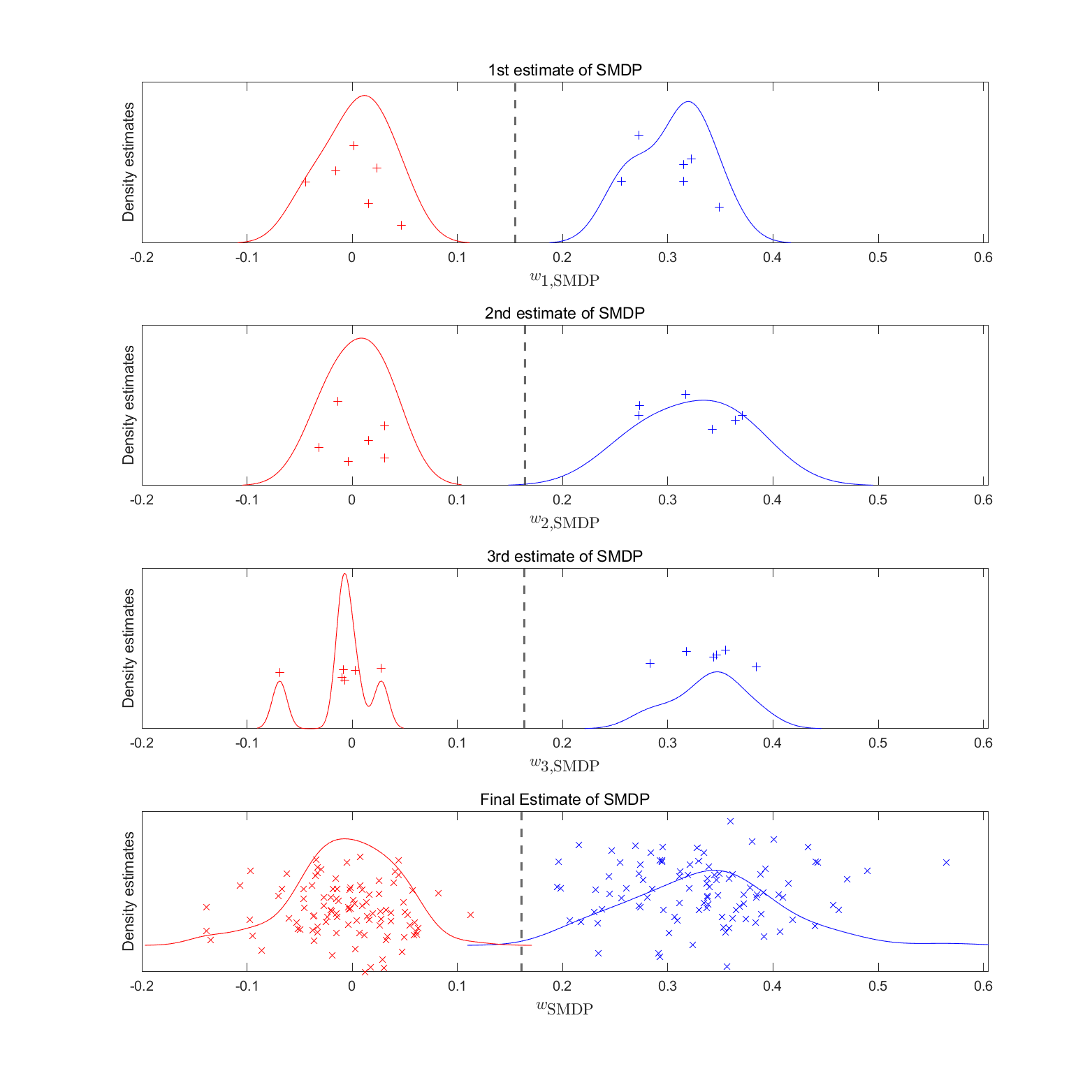
Figure 8: The first three panels show projections of $\mathcal{X}_{te}$ (class 1: blue pluses, class 2: red pluses) onto $w_{j,\textup{SMDP}}$ and classification threshold $b_{j}$ (dotted line) for $j=1,2,3$. The last panel shows projections of independent test data $\mathcal{Y}$ (class 1: blue crosses, class 2: red crosses) onto $w_{\textup{SMDP}}$ and final classification threshold $b_{\textup{SMDP}}$ (dotted line).

6 Simulation

In this section, we numerically show that $\phi_{\textup{MDP}}$ in (13), $\phi_{\textup{b-MDP}}$ in (14), $\phi_{\textup{PRD},\alpha}$ in (17), $\phi_{\textup{b-PRD},\alpha}$ in (26), $\phi_{\textup{SMDP-I}}$ in (21) and $\phi_{\textup{SMDP-II}}$ in (22) can achieve asymptotic perfect classification under various heterogeneous covariance models. We demonstrate that bias-corrected classification rules $\phi_{\textup{b-MDP}}$ and $\phi_{\textup{b-PRD},\alpha}$ with a negative ridge parameter achieve better classification performances than $\phi_{\textup{MDP}}$ and $\phi_{\textup{PRD},\alpha}$ for the cases of unequal tail eigenvalues. Also, we confirm that $\phi_{\textup{SMDP-I}}$ and $\phi_{\textup{SMDP-II}}$ achieve nearly perfect classification in various settings. We compare classification rates of these classification rules with those of weighted Distance Weighted Discrimination (wDWD) by Qiao et al. (2010), Support Vector Machine (SVM) by Vapnik (1995), Distance-Based Discriminant Analysis (DBDA) by Aoshima and Yata (2013), Transformed Distance-Based Discriminant Analysis (T-DBDA) by Aoshima and Yata (2019), the distance-based linear classifier using the data transformation procedure (DT) by Ishii (2020), Geometrical Quadratic Discriminant Analysis (GQDA) by Aoshima and Yata (2011) and Transformed Geometrical Quadratic Discriminant Analysis (T-GQDA) by Ishii et al. (2022).

Our model, which assumed to be satisfying Assumptions 1—5, is that $X_{kj}\sim\mathcal{N}_{p}(\mbox{\boldmath{$\mu$}}_{(k)},\mbox{\boldmath{$\Sigma$}}_{(k)})$ for $k=1,2$, $1\leq j\leq 20$ and $p=10,000$. We set $\mbox{\boldmath{$\mu$}}_{(1)}=p^{-1/2}(\sqrt{8}\mathbf{1}_{p/8}^{\top},\mathbf{0}_{7p/8}^{\top})^{\top}$, $\mbox{\boldmath{$\mu$}}_{(2)}=\mathbf{0}_{p}$. Note that in this case $\delta^{2}=1$. $\mbox{\boldmath{$\Sigma$}}_{(1)}$ and $\mbox{\boldmath{$\Sigma$}}_{(2)}$ will be given differently for each setting. We consider ten settings to reflect various covariance assumptions.

• $(\mbox{\boldmath{$\Sigma$}}_{(1)}=\mbox{\boldmath{$\Sigma$}}_{(2)})$ : In Setting I and Setting II, we assume two population have the common covariance matrix, that is,

  $$\mbox{\boldmath{$\Sigma$}}_{(1)}=\mbox{\boldmath{$\Sigma$}}_{(2)}=\sum\limits_{i=1}^{2}\sigma_{i}^{2}\mathbf{u}_{i}\mathbf{u}_{i}^{\top}+\tau^{2}\mathbf{I}_{p}$$

  where $(\sigma_{1}^{2},\sigma_{2}^{2})=(20p^{\beta},10p^{\beta})$,

  $$(\mathbf{u}_{1},\mathbf{u}_{2})=\frac{1}{\sqrt{p}}\begin{bmatrix}\sqrt{2}\mathbf{1}_{p/4}&\mathbf{0}_{p/4}\\ \sqrt{2}\mathbf{1}_{p/4}&\mathbf{0}_{p/4}\\ \mathbf{0}_{p/4}&\sqrt{2}\mathbf{1}_{p/4}\\ \mathbf{0}_{p/4}&\sqrt{2}\mathbf{1}_{p/4}\end{bmatrix}$$

  and $\tau^{2}=30$. We assume $\beta=1/2$ (then, $m=0$) in Setting I while $\beta=1$ (then, $m=2$) in Setting II.

• $(\mbox{\boldmath{$\Sigma$}}_{(1)}\neq\mbox{\boldmath{$\Sigma$}}_{(2)}$ and $\tau_{1}^{2}=\tau_{2}^{2})$ : In Setting III to Setting VI, we assume heterogeneous covariance models with equal tail eigenvalues, that is, $\tau_{1}^{2}=\tau_{2}^{2}=:\tau^{2}$. To be specific, in Setting III to Setting V, we assume

  $$\mbox{\boldmath{$\Sigma$}}_{(1)}=\sum\limits_{i=1}^{2}\sigma_{(1),i}^{2}\mathbf{u}_{(1),i}\mathbf{u}_{(1),i}^{\top}+\tau_{1}^{2}\mathbf{I}_{p}$$ (23)

  and

  $$\mbox{\boldmath{$\Sigma$}}_{(2)}=\sum\limits_{i=1}^{3}\sigma_{(2),i}^{2}\mathbf{u}_{(2),i}\mathbf{u}_{(2),i}^{\top}+\tau_{2}^{2}\mathbf{I}_{p}$$ (24)

  where $(\sigma_{(1),1}^{2},\sigma_{(1),2}^{2})=(20p^{\beta_{1}},10p^{\beta_{1}}),(\sigma_{(2),1}^{2},\sigma_{(2),2}^{2},\sigma_{(2),3}^{2})=(20p^{\beta_{2}},10p^{\beta_{2}},5p^{\beta_{2}})$,

  $$(\mathbf{u}_{(1),1},\mathbf{u}_{(1),2})=\frac{1}{\sqrt{p}}\begin{bmatrix}\sqrt{2}\mathbf{1}_{p/4}&\mathbf{0}_{p/4}\\ \sqrt{2}\mathbf{1}_{p/4}&\mathbf{0}_{p/4}\\ \mathbf{0}_{p/4}&\sqrt{2}\mathbf{1}_{p/4}\\ \mathbf{0}_{p/4}&\sqrt{2}\mathbf{1}_{p/4}\end{bmatrix},$$

  $$(\mathbf{u}_{(2),1},\mathbf{u}_{(2),2},\mathbf{u}_{(2),3})=\frac{1}{\sqrt{p}}\begin{bmatrix}\mathbf{1}_{p/4}&\sqrt{2}\mathbf{1}_{p/4}&\mathbf{0}_{p/4}\\ \mathbf{1}_{p/4}&\mathbf{0}_{p/4}&\sqrt{2}\mathbf{1}_{p/4}\\ \mathbf{1}_{p/4}&-\sqrt{2}\mathbf{1}_{p/4}&\mathbf{0}_{p/4}\\ \mathbf{1}_{p/4}&\mathbf{0}_{p/4}&-\sqrt{2}\mathbf{1}_{p/4}\end{bmatrix}$$

  and $\tau_{1}^{2}=\tau_{2}^{2}=:\tau^{2}=30$. We assume $(\beta_{1},\beta_{2})=(1/2,1/2)$ (then, $m=0$) in Setting III, $(\beta_{1},\beta_{2})=(1,1/2)$ (then, $m=2$) in Setting IV, $(\beta_{1},\beta_{2})=(1,1)$ (then, $m=3$) in Setting V. In Setting VI, we assume

  $$\mbox{\boldmath{$\Sigma$}}_{(1)}=\sum\limits_{i=1}^{3}\sigma_{(1),i}^{2}\mathbf{u}_{(1),i}\mathbf{u}_{(1),i}^{\top}+\tau_{1}^{2}\mathbf{I}_{p}$$ (25)

  where $\sigma_{(1),1}^{2},\sigma_{(1),2}^{2},\mathbf{u}_{(1),1},\mathbf{u}_{(1),2}$ and $\tau_{1}^{2}$ are same with those in $\mbox{\boldmath{$\Sigma$}}_{(1)}$ in (23), $\sigma_{(1),3}^{2}=5p^{\beta_{1}}$ and $\mathbf{u}_{(1),3}=p^{-1/2}(\mathbf{1}_{p/4}^{\top},-\mathbf{1}_{p/4}^{\top},\mathbf{1}_{p/4}^{\top},-\mathbf{1}_{p/4}^{\top})^{\top}$. Also, we continue to assume $\mbox{\boldmath{$\Sigma$}}_{(2)}$ in (24) and $(\beta_{1},\beta_{2})=(1,1)$ (then, $m=4$) in Setting VI. Note that in Setting VI, $m>\max{(m_{1},m_{2})}$ in contrast to Setting V where $m=m_{2}$.

• $(\mbox{\boldmath{$\Sigma$}}_{(1)}\neq\mbox{\boldmath{$\Sigma$}}_{(2)}$ and $\tau_{1}^{2}>\tau_{2}^{2})$ : In Setting VII to Setting X, we assume heterogeneous covariance models with unequal tail eigenvalues, that is, $\tau_{1}^{2}>\tau_{2}^{2}$. To be specific, in Setting VII to Setting IX, we continue to assume $\mbox{\boldmath{$\Sigma$}}_{(1)}$ in (23) and $\mbox{\boldmath{$\Sigma$}}_{(2)}$ in (24) but $\tau_{1}^{2}=30$ and $\tau_{2}^{2}=15$. We assume $(\beta_{1},\beta_{2})=(1/2,1/2)$ (then, $m=0$) in Setting VII, $(\beta_{1},\beta_{2})=(1,1/2)$ (then, $m=2$) in Setting VIII, $(\beta_{1},\beta_{2})=(1,1)$ (then, $m=3$) in Setting IX. In Setting X, we continue to assume $\mbox{\boldmath{$\Sigma$}}_{(1)}$ in (25) and $\mbox{\boldmath{$\Sigma$}}_{(2)}$ in (24) but $\tau_{1}^{2}=30$ and $\tau_{2}^{2}=15$. We assume $(\beta_{1},\beta_{2})=(1,1)$ (then, $m=4$) in Setting X. Note that in Setting X, $m>\max{(m_{1},m_{2})}$ in contrast to Setting IX where $m=m_{2}$.

For Settings II, IV and VIII where $(\beta_{1},\beta_{2})=(1,1/2)$ and $m=2$, note that $\cos^{2}\varphi=1/4$. For Settings V, IX where $(\beta_{1},\beta_{2})=(1,1)$ and $m=3$, $\cos^{2}\varphi=3/8$. For Settings VI, X where $(\beta_{1},\beta_{2})=(1,1)$ and $m=4$, $\cos^{2}\varphi=1/2$.

To clearly check classification performances of each classification rule, we use the true numbers of $m_{1}$, $m_{2}$ and $m$ for $\phi_{\textup{PRD},\hat{\alpha}}$, $\phi_{\textup{b-PRD},\hat{\alpha}_{1}}$, $\phi_{\textup{b-PRD},\hat{\alpha}_{2}}$ ($\hat{\alpha}$, $\hat{\alpha}_{1}$ and $\hat{\alpha}_{2}$ are defined in (15) and (27)), $\phi_{\textup{SMDP-I}}$ and $\phi_{\textup{SMDP-II}}$. Also, we use the true number of strongly spiked eigenvalues for T-DBDA (Aoshima and Yata, 2019) and T-GQDA (Ishii et al., 2022). For $\phi_{\textup{SMDP-I}}$ and $\phi_{\textup{SMDP-II}}$, we set $n_{1,te}=n_{2,te}=6$ so that $\mathcal{X}_{te}$ consists of $30\%$ of original training data $\mathcal{X}$. The classification rates are obtained using $1,000$ independent observations ($500$ independent observations for each class). We repeat this procedure $100$ times and average classification rates to estimate classification accuracy of each classification rule. Table 2 provides a summary of our simulation settings. Table 3 shows all simulation results from Setting I to Setting X and these results are consistent with the theoretical findings in Sections 4 and 5.

Note that both of $\phi_{\textup{MDP}}$ and $\phi_{\textup{b-MDP}}$ achieve nearly perfect classification in Settings I and III where $\mbox{\boldmath{$\Sigma$}}_{(1)}$ and $\mbox{\boldmath{$\Sigma$}}_{(2)}$ have weak spikes and equal tail eigenvalues. However, only $\phi_{\textup{b-MDP}}$ achieves nearly perfect classification in Setting VII where two covariance matrices have weak spikes but unequal tail eigenvalues. These classification rules do not achieve perfect classification in the other settings where $\mbox{\boldmath{$\Sigma$}}_{(1)}$ or $\mbox{\boldmath{$\Sigma$}}_{(2)}$ has strong spikes.

Setting	($\mbox{\boldmath{$\Sigma$}}_{(1)},\mbox{\boldmath{$\Sigma$}}_{(2)}$)	($\tau_{1}^{2},\tau_{2}^{2}$)	($\beta_{1},\beta_{2}$)	$m$	$\phi_{\textup{MDP}}$	$\phi_{\textup{b-MDP}}$	$\phi_{\textup{PRD},\hat{\alpha}}$	$\phi_{\textup{b-PRD},\hat{\alpha}_{1}}$	$\phi_{\textup{b-PRD},\hat{\alpha}_{2}}$	$\phi_{\textup{SMDP-I}}$	$\phi_{\textup{SMDP-II}}$
I	$\mbox{\boldmath{$\Sigma$}}_{(1)}=\mbox{\boldmath{$\Sigma$}}_{(2)}$	$\tau_{1}^{2}=\tau_{2}^{2}$	$(1/2,1/2)$	$m=0$	O	O	O	O	O	O	O
II			$(1,1)$	$m=m_{1}=m_{2}$	X	X	O	O	O	O	O
III	$\mbox{\boldmath{$\Sigma$}}_{(1)}\neq\mbox{\boldmath{$\Sigma$}}_{(2)}$	$\tau_{1}^{2}=\tau_{2}^{2}$	$(1/2,1/2)$	$m=0$	O	O	O	O	O	O	O
IV			$(1,1/2)$	$m=m_{1}$	X	X	O	O	O	O	O
V			$(1,1)$	$m=m_{2}$	X	X	O	O	O	O	O
VI			$(1,1)$	$m>\max{(m_{1},m_{2})}$	X	X	O	O	O	O	O
VII	$\mbox{\boldmath{$\Sigma$}}_{(1)}\neq\mbox{\boldmath{$\Sigma$}}_{(2)}$	$\tau_{1}^{2}\neq\tau_{2}^{2}$	$(1/2,1/2)$	$m=0$	X	O	X	O	O	O	O
VIII			$(1,1/2)$	$m=m_{1}$	X	X	X	O	X	O	O
IX			$(1,1)$	$m=m_{2}$	X	X	X	X	O	O	O
X			$(1,1)$	$m>\max{(m_{1},m_{2})}$	X	X	X	X	X	O	O

Table 2: Classification rules that theoretically achieve perfect classification in each setting are marked as ‘O’, while the others are marked as ‘X’.

Setting	MDP		PRD			SMDP
	$\phi_{\textup{MDP}}$	$\phi_{\textup{b-MDP}}$	$\phi_{\textup{PRD},\hat{\alpha}}$	$\phi_{\textup{b-PRD},\hat{\alpha}_{1}}$	$\phi_{\textup{b-PRD},\hat{\alpha}_{2}}$	$\phi_{\textup{SMDP-I}}$		$\phi_{\textup{SMDP-II}}$		wDWD	SVM	T-DBDA	DT	T-GQDA
						$K=5$	$K=10$	$K=5$	$K=10$
I	0.9846	0.9846	0.9846	0.9846	0.9846	0.9807	0.9809	0.9801	0.9807	0.9807	0.9846	0.9961	0.9936	0.9808
	0.0012	0.0013	0.0012	0.0013	0.0013	0.0013	0.0014	0.0014	0.0014	0.0014	0.0012	0.0005	0.0010	0.0010
II	0.8589	0.8590	0.9995	0.9995	0.9995	0.9989	0.9993	0.9988	0.9992	0.7012	0.8585	0.7837	0.5807	0.6782
	0.0102	0.0102	0.0001	0.0001	0.0001	0.0001	0.0001	0.0001	0.0001	0.0097	0.0103	0.0101	0.0073	0.0083
III	0.9809	0.9811	0.9809	0.9811	0.9811	0.9776	0.9779	0.9773	0.9777	0.9779	0.9809	0.9916	0.9823	0.9764
	0.0012	0.0012	0.0012	0.0012	0.0012	0.0013	0.0014	0.0014	0.0014	0.0014	0.0012	0.0006	0.0015	0.0010
IV	0.8759	0.8766	0.9962	0.9961	0.9961	0.9932	0.9947	0.9930	0.9949	0.8177	0.8759	0.8295	0.7504	0.9464
	0.0067	0.0067	0.0003	0.0003	0.0003	0.0007	0.0004	0.0010	0.0005	0.0072	0.0067	0.0134	0.0046	0.0075
V	0.7917	0.7918	0.9964	0.9964	0.9964	0.9918	0.9942	0.9919	0.9940	0.6548	0.7912	0.7014	0.5559	0.7527
	0.0091	0.0091	0.0003	0.0003	0.0003	0.0006	0.0005	0.0006	0.0005	0.0070	0.0092	0.0074	0.0048	0.0066
VI	0.7281	0.7281	0.9824	0.9826	0.9823	0.9677	0.9746	0.9657	0.9742	0.6217	0.7275	0.6536	0.5501	0.8698
	0.0076	0.0076	0.0008	0.0008	0.0009	0.0018	0.0014	0.0019	0.0014	0.0055	0.0077	0.0055	0.0041	0.0042
VII	0.8373	0.9876	0.8373	0.9876	0.9876	0.9843	0.9844	0.9839	0.9842	0.8402	0.8373	0.9960	0.9881	1.0000
	0.0035	0.0010	0.0035	0.0010	0.0010	0.0011	0.0012	0.0012	0.0012	0.0035	0.0035	0.0005	0.0014	0.0000
VIII	0.7255	0.8785	0.7264	0.9991	0.9386	0.9980	0.9987	0.9975	0.9985	0.7231	0.7258	0.8533	0.7595	0.9989
	0.0029	0.0068	0.0039	0.0001	0.0054	0.0004	0.0002	0.0006	0.0003	0.0029	0.0028	0.0143	0.0062	0.0004
IX	0.6981	0.8579	0.6361	0.9518	0.9989	0.9989	0.9993	0.9988	0.9993	0.6486	0.6963	0.7032	0.5560	0.9757
	0.0038	0.0089	0.0039	0.0085	0.0036	0.0001	0.0001	0.0001	0.0001	0.0062	0.0040	0.0755	0.0484	0.0254
X	0.6689	0.7823	0.5755	0.9181	0.9508	0.9902	0.9931	0.9891	0.9928	0.6197	0.6673	0.6543	0.5501	0.9909
	0.0036	0.0080	0.0036	0.0102	0.0060	0.0007	0.0005	0.0009	0.0006	0.0048	0.0037	0.0056	0.0042	0.0012

Table 3: Estimates of the classification accuracy of Setting I to Setting X are given in the first row of each cell, and standard errors are given in the second row of each cell.

Also, all of $\phi_{\textup{PRD},\hat{\alpha}}$, $\phi_{\textup{b-PRD},\hat{\alpha}_{1}}$ and $\phi_{\textup{b-PRD},\hat{\alpha}_{2}}$ achieve nearly perfect classification in Settings I—VI where $\mbox{\boldmath{$\Sigma$}}_{(1)}$ and $\mbox{\boldmath{$\Sigma$}}_{(2)}$ have equal tail eigenvalues even when they have strong spikes. However, $\phi_{\textup{PRD},\hat{\alpha}}$ does not achieve perfect classification if $\mbox{\boldmath{$\Sigma$}}_{(1)}$ and $\mbox{\boldmath{$\Sigma$}}_{(2)}$ have unequal tail eigenvalues. For example, $\phi_{\textup{b-PRD},\hat{\alpha}_{1}}$ and $\phi_{\textup{b-PRD},\hat{\alpha}_{2}}$ achieves nearly perfect classification in Setting VII, where $\mbox{\boldmath{$\Sigma$}}_{(1)}$ and $\mbox{\boldmath{$\Sigma$}}_{(2)}$ have weak spikes and unequal tail eigenvalues while $\phi_{\textup{PRD},\hat{\alpha}}$ does not (in fact, $\phi_{\textup{b-PRD},\alpha}$ achieves perfect classification for all $\alpha\in\mathbb{R}$ in this setting). Also, only $\phi_{\textup{b-PRD},\hat{\alpha}_{1}}$ achieves nearly perfect classification in Setting VIII where only $\mbox{\boldmath{$\Sigma$}}_{(1)}$ has strong spikes and $\mbox{\boldmath{$\Sigma$}}_{(1)}$ and $\mbox{\boldmath{$\Sigma$}}_{(2)}$ have unequal eigenvalues. Note that $\phi_{\textup{b-PRD},\hat{\alpha}_{2}}$ do not achieve perfect classification in this setting, since $\phi_{\textup{b-PRD},\alpha}$ achieves perfect classification only with the negative ridge parameter $\alpha:=\hat{\alpha}_{1}$ (see Theorem 40 in Appendix B). In contrast, in Setting IX, only $\phi_{\textup{b-PRD},\hat{\alpha}_{2}}$ achieves nearly perfect classification while $\phi_{\textup{b-PRD},\hat{\alpha}_{1}}$ do not, since in this setting the leading eigenspace of the second class includes that of the first class (that is, $m=m_{2}>m_{1}$) (see Appendix A). However, both of $\phi_{\textup{b-PRD},\hat{\alpha}_{1}}$ and $\phi_{\textup{b-PRD},\hat{\alpha}_{2}}$ do not achieve nearly perfect classification in Setting X, where $\mbox{\boldmath{$\Sigma$}}_{(1)}$ and $\mbox{\boldmath{$\Sigma$}}_{(2)}$ have strong spikes, unequal eigenvalues and $m>\max{(m_{1},m_{2})}$.

We can check that $\phi_{\textup{SMDP-I}}$ and $\phi_{\textup{SMDP-II}}$ achieve nearly perfect classification in all of the settings. Note that in Setting X, only $\phi_{\textup{SMDP-I}}$ and $\phi_{\textup{SMDP-II}}$ achieve nearly perfect classification among the classification rules except T-GQDA by Ishii et al. (2022). These results confirm that our approach, projecting $w_{\textup{MDP}}$ onto the nullspace of the common leading eigenspace, successfully work under various heterogeneous covariance models.

We exclude the results of DBDA by Aoshima and Yata (2013) and GQDA by Aoshima and Yata (2011), since T-DBDA by Aoshima and Yata (2019) and T-GQDA by Ishii et al. (2022) show better performances than these classification rules in all settings. It implies that the data transformation technique, which removes excessive variability within the leading eigenspace, contributes to achieve better classification performances when $\mbox{\boldmath{$\Sigma$}}_{(1)}$ or $\mbox{\boldmath{$\Sigma$}}_{(2)}$ has meaningfully diverging components. In particular, T-GQDA achieves nearly perfect classification in Setting VII—X where $\mbox{\boldmath{$\Sigma$}}_{(1)}\neq\mbox{\boldmath{$\Sigma$}}_{(2)}$ and $\tau_{1}^{2}\neq\tau_{2}^{2}$. However, these classification rules and DT (Ishii, 2020) estimate the structure of the leading eigenspace of each class, which may degrade classification performances when the sample size is small but the data has strong signals as in our simulation models.

A Bias-corrected projected ridge classification rule

In this section, we provide a bias-corrected projected ridge classification rule, which is a bias-corrected version of $\phi_{\textup{PRD},\alpha}$ in (17).

For the case of strong spikes with unequal tail eigenvalues, Propositions 15 and 21 state that $v_{\hat{\alpha}_{k}}^{c}$ is asymptotically orthogonal to $\mathbf{u}_{(k),1}$, which is the leading eigenvector of the $k$th class if $m_{1}=m_{2}=1$. These results can be extended to the general cases where $m_{1}\geq 1$ and $m_{2}\geq 1$. Theorem 29 tells that the ‘conditioned’ projected ridged linear discriminant vector $v_{\hat{\alpha}_{k}}^{c}$ is asymptotically orthogonal to $\mathcal{U}_{(k)}$, which is the leading eigenspace of the $k$th class.

Theorem 29

Suppose Assumptions 1—5 hold and assume $\beta_{1}=\beta_{2}=1$ and $\tau_{1}^{2}>\tau_{2}^{2}$. For any given training data $\mathcal{X}$ and $\hat{\alpha}_{k}$ chosen as an HDLSS-consistent estimator of $-\tau_{k}^{2}$, $\mbox{Angle}{(v_{\hat{\alpha}_{k}}^{c},\mathbf{u}_{(k),i,\mathcal{S}})}\xrightarrow{P}\pi/2$ as $p\to\infty$ for $k=1,2$ and $1\leq i\leq m_{k}$.

Since $v_{\hat{\alpha}_{k}}^{c}$ is asymptotically orthogonal to ${\rm span}(\mathbf{U}_{(k),1,\mathcal{S}})$, $P_{v_{\hat{\alpha}_{k}}^{c}}\mathcal{Y}_{k}$ converges to a single point as $p$ increases for each $k=1,2$. It implies that if $\mathcal{U}_{(1)}$ includes $\mathcal{U}_{(2)}$ (or $\mathcal{U}_{(2)}$ includes $\mathcal{U}_{(1)}$), then both of $\mathcal{Y}_{1}$ and $\mathcal{Y}_{2}$ are piled on $v_{\hat{\alpha}_{1}}^{c}$ (or $v_{\hat{\alpha}_{2}}^{c}$), respectively.

Theorem 30

Suppose Assumptions 1—5 hold and assume $\beta_{1}=\beta_{2}=1$, $\tau_{1}^{2}>\tau_{2}^{2}$. Also, for $1\leq k\neq s\leq 2$, further assume that $m=m_{k}\geq m_{s}$ (that is, $\mathcal{U}_{(k)}$ includes $\mathcal{U}_{(s)}$). Then

$$\frac{1}{\sqrt{p}}v_{\hat{\alpha}_{k}}^{c\top}(Y-\bar{X})\xrightarrow{P}\begin{cases}\gamma_{k}(\eta_{2}(1-\cos^{2}\varphi)\delta^{2}-(\tau_{1}^{2}-\tau_{2}^{2})/n),&\pi(Y)=1,\\ \gamma_{k}(-\eta_{1}(1-\cos^{2}\varphi)\delta^{2}-(\tau_{1}^{2}-\tau_{2}^{2})/n),&\pi(Y)=2\end{cases}$$

as $p\to\infty$ where $\gamma_{k}$ is a strictly positive random variable depending on the true principal component scores of $\mathcal{X}$.

See (72) and (73) in Appendix D for definitions of $\gamma_{1}$ and $\gamma_{2}$.

Note that Theorem 30 is a generalized version of Proposition 16. For the case of strong spikes with unequal eigenvalues, if $m=m_{k}$, Theorem 30 tells that $v_{\hat{\alpha}_{k}}^{c}$ is a second data piling direction. It implies that if $m=m_{1}$, then both $v_{\hat{\alpha}_{1}}$ can yield perfect classification since $v_{\hat{\alpha}_{1}}=v_{\hat{\alpha}_{1}}^{c}$. Also, if $m=m_{2}$, then $v_{\hat{\alpha}_{2}}$ also yields perfect classification since $\|v_{\hat{\alpha}_{2}}-v_{\hat{\alpha}_{2}}^{c}\|\xrightarrow{P}0$ as $p\to\infty$. In the following, we introduce the bias-corrected projected ridge classification rule.

Bias-corrected projected ridge classification rule

We define the bias-corrected projected ridge classification rule as

$$\phi_{\textup{b-PRD},\alpha}(Y;\mathcal{X})=\begin{cases}1,&p^{-1/2}v_{\alpha}^{\top}(Y-\bar{X})-(\hat{\alpha}_{1}-\hat{\alpha}_{2})/(n\|\tilde{v}_{\alpha}\|)\geq 0,\\ 2,&p^{-1/2}v_{\alpha}^{\top}(Y-\bar{X})-(\hat{\alpha}_{1}-\hat{\alpha}_{2})/(n\|\tilde{v}_{\alpha}\|)<0,\end{cases}$$ (26)

where $\tilde{v}_{\alpha}$ is given as

$$\tilde{v}_{\alpha}=\sum\limits_{i\in\mathcal{D}}\frac{\alpha_{p}}{\hat{\lambda}_{i}+\alpha_{p}}\hat{\mathbf{u}}_{i}\left(\frac{1}{\sqrt{p}}\hat{\mathbf{u}}_{i}^{\top}\mathbf{d}\right)+\frac{1}{\sqrt{p}}\hat{\mathbf{U}}_{2}\hat{\mathbf{U}}_{2}^{\top}\mathbf{d}.$$

Note that $v_{\alpha}\varpropto\tilde{v}_{\alpha}$. We can show that $\|\tilde{v}_{\hat{\alpha}_{k}}\|\xrightarrow{P}\gamma_{k}^{-1}$ as $p\to\infty$ for $k=1,2$ if $\beta_{1}=\beta_{2}=1$ and $\tau_{1}^{2}>\tau_{2}^{2}$ (See Appendix D). Also, $\hat{\alpha}_{1}$ and $\hat{\alpha}_{2}$ can be obtained purely from training data $\mathcal{X}$. Note that $\hat{\lambda}_{(k),i}/p\xrightarrow{P}\tau_{k}^{2}$ as $p\to\infty$ for $m_{k}+1\leq i\leq n_{k}-1$ where $\hat{\lambda}_{(k),i}$ is $i$th largest eigenvalue of $\mathbf{S}_{k}$ (Jung et al., 2012). Based on this fact, from now on, we fix

$$\hat{\alpha}_{k}=-\frac{1}{n_{k}-m_{k}-1}\sum_{i=m_{k}+1}^{n_{k}-1}\frac{\hat{\lambda}_{(k),i}}{p}$$ (27)

for $k=1,2$. From Theorem 30, we can check that $\phi_{\textup{b-PRD},\hat{\alpha}_{1}}$ achieves perfect classification if $m=m_{1}$, and $\phi_{\textup{b-PRD},\hat{\alpha}_{2}}$ achieves perfect classification if $m=m_{2}$.

B Double Data Piling for the Case of Strong and Weak Spikes

In this section, we show that double data piling phenomenon also occurs for the cases where only one class has meaningfully diverging components while the other class does not, that is, $(i)$ $\beta_{1}=1$ and $\beta_{2}<1$ or $(ii)$ $\beta_{1}<1$ and $\beta_{2}=1$. Furthermore, we show that the projected ridged linear discriminant vector $v_{\alpha}$ with a negative ridge parameter $\alpha=-\tau_{1}^{2}$ or $\alpha=-\tau_{2}^{2}$ can be a second maximal data piling direction for these cases. As stated in Section 2, allowing $\beta_{k}<1$ results in similar asymptotic results as $m_{k}=0$ in Assumption 2 for $k=1,2$.

B.1 Data Piling of Independent Test Data

We investigate data piling phenomenon of independent test data under the one-component covariance model as in Section 3.1, but we consider the cases where $(i)$ $\beta_{1}=1$ and $\beta_{2}<1$ or $(ii)$ $\beta_{1}<1$ and $\beta_{2}=1$ in (28).

$$\mbox{\boldmath{$\Sigma$}}_{(1)}=\sigma_{(1),1}^{2}p^{\beta_{1}}\mathbf{u}_{(1),1}\mathbf{u}_{(1),1}^{\top}+\tau_{1}^{2}\mathbf{I}_{p};$$ (28)

$$\mbox{\boldmath{$\Sigma$}}_{(2)}=\sigma_{(2),1}^{2}p^{\beta_{2}}\mathbf{u}_{(2),1}\mathbf{u}_{(2),1}^{\top}+\tau_{2}^{2}\mathbf{I}_{p}.$$

First, we assume that both covariance matrices have equal tail eigenvalues, that is, $\tau_{1}^{2}=\tau_{2}^{2}$.

Example 5

We assume $\mathbf{u}_{(1),1}=\mathbf{u}_{(2),1}=:\mathbf{u}_{1}$, $\tau_{1}^{2}=\tau_{2}^{2}=:\tau^{2}$ and $(i)$ $\beta_{1}=1$ and $\beta_{2}<1$ in (28). In this case, the angle between $\hat{\mathbf{u}}_{1}$ and $\mathbf{u}_{1}$ does not degenerate, while the other sample eigenvectors $\hat{\mathbf{u}}_{2},\ldots,\hat{\mathbf{u}}_{n-2}$ are strongly inconsistent with $\mathbf{u}_{1}$, thus let $\mathcal{D}=\left\{1\right\}$.

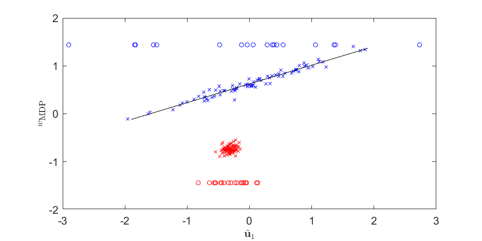
Figure 9: $2$-dimensional projections onto $\mathcal{S}={\rm span}(\left\{\hat{\mathbf{u}}_{i}\right\}_{i\in\mathcal{D}},w_{\textup{MDP}})$ with $\mathcal{D}=\left\{1\right\}$ of training data $\mathcal{X}$ (class 1: blue circles, class 2: red circles) and independent test data $\mathcal{Y}$ (class 1: blue crosses, class 2: red crosses) under the model in Example 5.

In Figure 9, independent test data $\mathcal{Y}_{1}$ are concentrated along straight line while $\mathcal{Y}_{2}$ converges to a single point in $\mathcal{S}={\rm span}(\left\{\hat{\mathbf{u}}_{i}\right\}_{i\in\mathcal{D}},w_{\textup{MDP}})={\rm span}(\hat{\mathbf{u}}_{1},w_{\textup{MDP}})$. Notice that the line formed by $\mathcal{Y}_{1}$ gives a meaningful distance from the point formed by $\mathcal{Y}_{2}$. Thus, we can find a line that passes through the point formed by $\mathcal{Y}_{2}$ and is parallel to the line formed by $\mathcal{Y}_{1}$. It can be shown that this line is asymptotically parallel to $P_{\mathcal{S}}\mathbf{u}_{1}$, which is the projection of the leading eigenvector of the first class $\mathbf{u}_{1}$ onto $\mathcal{S}$. In case where $\mathbf{u}_{(1),1}\neq\mathbf{u}_{(2),1}$, similar results are obtained since variation along $\mathbf{u}_{(2),1}$ is negligible.

The following proposition states that projections of $\mathcal{Y}$ onto $2$-dimensional subspace $\mathcal{S}={\rm span}(\hat{\mathbf{u}}_{1},w_{\textup{MDP}})$ are distributed along two lines, which become parallel to each other, and to $P_{\mathcal{S}}\mathbf{u}_{1}$, as $p$ increases.

Proposition 31

Suppose Assumptions 1—5 hold and assume $\beta_{1}=1$, $\beta_{2}<1$, $\tau_{1}^{2}=\tau_{2}^{2}$ and $m_{1}=m_{2}=1$. Also, let $\mathcal{S}={\rm span}(\hat{\mathbf{u}}_{1},w_{\textup{MDP}})$ and

$$L_{k}=\left\{\mathbf{u}_{1,{\mathcal{S}}}t+\nu_{k}w_{\textup{MDP}}+\bar{X}_{\mathcal{S}}:t\in\mathbb{R}\right\}$$

for $k=1,2$ where $\nu_{1}=\kappa_{\textup{MDP}}^{-1}\left(\eta_{2}(1-\cos^{2}\varphi)\delta^{2}\right)$ and $\nu_{2}=\kappa_{\textup{MDP}}^{-1}\left(-\eta_{1}(1-\cos^{2}\varphi)\delta^{2}\right)$. Then, for any independent observation $Y\in\mathcal{Y}$ and for any $\epsilon>0$,

$$\lim\limits_{p\to\infty}\mathbb{P}\left(\inf\limits_{a\in L_{k}}\|Y_{\mathcal{S}}-a\|>\epsilon|\pi(Y)=k\right)=0$$

for $k=1,2$.

Note that projections of $\mathcal{Y}_{1}$ are concentrated along the line $L_{1}$, while $\mathcal{Y}_{2}$ are piled on some point on the line $L_{2}$, which is parallel to $L_{1}$. Allowing $\beta_{1}<1$ and $\beta_{2}=1$ also brings similar results with Proposition 31. In this case, projections of $\mathcal{Y}_{2}$ is concentrated along the line $L_{2}$, while $\mathcal{Y}_{1}$ is piled on some point on the line $L_{1}$, which is parallel to $L_{2}$.

We now investigate the case of $\tau_{1}^{2}\neq\tau_{2}^{2}$. Without loss of generality, we assume $\tau_{1}^{2}>\tau_{2}^{2}$. Even in this case, the conclusion of Proposition 31 also holds for the setting $(i)$ $\beta_{1}=1$, $\beta_{2}<1$, as long as $\nu_{1}$ and $\nu_{2}$ in Proposition 31 are replaced by $\nu_{1}=\kappa_{\textup{MDP}}^{-1}\left(\eta_{2}(1-\cos^{2}\varphi)\delta^{2}-(\tau_{1}^{2}-\tau_{2}^{2})/n\right)$ and $\nu_{2}=\kappa_{\textup{MDP}}^{-1}\left(-\eta_{1}(1-\cos^{2}\varphi)\delta^{2}-(\tau_{1}^{2}-\tau_{2}^{2})/n\right)$. However, the assumption $\tau_{1}^{2}>\tau_{2}^{2}$ now makes a difference for the setting $(ii)$ $\beta_{1}<1$ and $\beta_{2}=1$.

Example 6

We assume $\mathbf{u}_{(1),1}=\mathbf{u}_{(2),1}=:\mathbf{u}_{1}$, $\tau_{1}^{2}>\tau_{2}^{2}$ and $(ii)$ $\beta_{1}<1$ and $\beta_{2}=1$ in (28). In this case, the important variation along $\mathbf{u}_{1}$ can be captured by either $\hat{\mathbf{u}}_{1}$ or $\hat{\mathbf{u}}_{n_{1}}$. To be specific, when the variation along $\mathbf{u}_{1}$ in the data from the second class is smaller than the variance $\tau_{1}^{2}$ of the first class, then $\hat{\mathbf{u}}_{n_{1}}$ explains the variation while $\hat{\mathbf{u}}_{1},\ldots,\hat{\mathbf{u}}_{n_{1}-1}$ explain the deterministic simplex with edge length $\sqrt{2}\tau_{1}\sqrt{p}$ for data only from the first class. The rest of sample eigenvectors $\hat{\mathbf{u}}_{n_{1}+1},\ldots,\hat{\mathbf{u}}_{n-2}$ explain the deterministic simplex with edge length $\sqrt{2}\tau_{2}\sqrt{p}$ for data only from the second class. On the other hand, if the sample variance of projection scores along $\mathbf{u}_{1}$ is larger than $\tau_{1}^{2}$, then $\hat{\mathbf{u}}_{1}$ explains the variation along $\mathbf{u}_{1}$ in the data instead of $\hat{\mathbf{u}}_{n_{1}}$. Hence, let $\mathcal{D}=\left\{1,n_{1}\right\}$.

Figure 10: $2$-dimensional projections onto $\mathcal{S}_{n_{1}}={\rm span}(\hat{\mathbf{u}}_{n_{1}},w_{\textup{MDP}})$ of training data $\mathcal{X}$ (class 1: blue circles, class 2: red circles) and independent test data $\mathcal{Y}$ (class 1: blue crosses, class 2: red crosses) under the model in Example 6.

In Figure 10, we observe that independent test data $\mathcal{Y}_{2}$ forms a straight line while $\mathcal{Y}_{1}$ converges to a point in $\mathcal{S}_{n_{1}}={\rm span}(\hat{\mathbf{u}}_{n_{1}},w_{\textup{MDP}})$, and the line and the point do not overlap. It turns out the direction of the straight line in $\mathcal{S}_{n_{1}}$ is parallel to $P_{\mathcal{S}_{n_{1}}}\mathbf{u}_{1}$, which is the projection of the leading eigenvector $\mathbf{u}_{1}$ onto $\mathcal{S}_{n_{1}}$. It implies that important variation of data from the second class is captured by $\hat{\mathbf{u}}_{n_{1}}$.

We remark that we can observe the separation of two groups of test data on $\mathcal{S}_{1}$ instead of $\mathcal{S}_{n_{1}}$ depending on the true leading principal component scores of the data from the second class. However, we can always observe this phenomenon in $\mathcal{S}={\rm span}(\left\{\hat{\mathbf{u}}_{i}\right\}_{i\in\mathcal{D}},w_{\textup{MDP}})$. In case where $\mathbf{u}_{(1),1}\neq\mathbf{u}_{(2),1}$, similar results are obtained since the variation along $\mathbf{u}_{(1),1}$ is negligible.

The following proposition states that even if $\tau_{1}^{2}>\tau_{2}^{2}$, projections of $\mathcal{Y}$ onto $\mathcal{S}$, which is a low-dimensional subspace of $\mathcal{S}_{X}$, are distributed along two parallel lines as $p$ increases. However, in this case, $\mathcal{S}$ may not be ${\rm span}(\hat{\mathbf{u}}_{1},w_{\textup{MDP}})$.

Proposition 32

Suppose Assumptions 1—5 hold. Also, assume $\beta_{1}<1$, $\beta_{2}=1$, $\tau_{1}^{2}>\tau_{2}^{2}$ and $m_{1}=m_{2}=1$. Also, let $\mathcal{S}={\rm span}(\hat{\mathbf{u}}_{1},\hat{\mathbf{u}}_{n_{1}},w_{\textup{MDP}})$ and

$$L_{k}=\left\{\mathbf{u}_{1,{\mathcal{S}}}t+\nu_{k}w_{\textup{MDP}}+\bar{X}_{\mathcal{S}}:t\in\mathbb{R}\right\}$$

for $k=1,2$ where $\nu_{1}=\kappa_{\textup{MDP}}^{-1}(\eta_{2}(1-\cos^{2}\varphi)\delta^{2}-(\tau_{1}^{2}-\tau_{2}^{2})/n)$ and $\nu_{2}=\kappa_{\textup{MDP}}^{-1}(-\eta_{1}(1-\cos^{2}\varphi)\delta^{2}-(\tau_{1}^{2}-\tau_{2}^{2})/n).$ Then, for any independent observation $Y\in\mathcal{Y}$ and for any $\epsilon>0$,

$$\lim\limits_{p\to\infty}\mathbb{P}\left(\inf\limits_{a\in L_{k}}\|Y_{\mathcal{S}}-a\|>\epsilon|\pi(Y)=k\right)=0$$

for $k=1,2$.

From Examples 5 and 6, we can check that projections of independent test data $\mathcal{Y}_{k}$ onto $\mathcal{S}$ tend to lie on a line if $\beta_{k}=1$, or a point if $\beta_{k}<1$. The signal subspace $\mathcal{S}$ was either ${\rm span}(\hat{\mathbf{u}}_{1},w_{\textup{MDP}})$ or ${\rm span}(\hat{\mathbf{u}}_{1},\hat{\mathbf{u}}_{n_{1}},w_{\textup{MDP}})$. To determine the signal subspace $\mathcal{S}$ for general cases where $m_{1}\geq 1$ and $m_{2}\geq 1$, we investigate the asymptotic behavior of sample eigenvalues and eigenvectors of $\mathbf{S}_{W}$. Recall that we assume $\tau_{1}^{2}\geq\tau_{2}^{2}$.

Lemma 33

Suppose Assumptions 1—5 hold. Then, the following hold as $p\to\infty$.

• If $\beta_{1}=1$ and $0\leq\beta_{2}<1$, then conditional on $\mathbf{W}_{(1)}$ and $\mathbf{W}_{(2)}$,

  $$p^{-1}\hat{\lambda}_{i}\xrightarrow{P}\begin{cases}\phi_{i}(\mbox{\boldmath{$\Phi$}}_{1})+\tau_{1}^{2},&1\leq i\leq m_{1},\\ \tau_{1}^{2},&m_{1}+1\leq i\leq n_{1}-1,\\ \tau_{2}^{2},&n_{1}\leq i\leq n-2.\end{cases}$$

• If $0\leq\beta_{1}<1$ and $\beta_{2}=1$, then conditional on $\mathbf{W}_{(1)}$ and $\mathbf{W}_{(2)}$,

  $$p^{-1}\hat{\lambda}_{i}\xrightarrow{P}\begin{cases}\phi_{i}(\mbox{\boldmath{$\Phi$}}_{2})+\tau_{2}^{2},&1\leq i\leq k_{1},\\ \tau_{1}^{2},&k_{1}+1\leq i\leq k_{1}+(n_{1}-1),\\ \phi_{i-(n_{1}-1)}(\mbox{\boldmath{$\Phi$}}_{2})+\tau_{2}^{2},&k_{1}+n_{1}\leq i\leq n_{1}+m_{2}-1,\\ \tau_{2}^{2},&n_{1}+m_{2}\leq i\leq n-2,\end{cases}$$

  where $k_{1}$ $(0\leq k_{1}\leq m_{2})$ is an integer which satisfies $\phi_{k_{1}}(\mbox{\boldmath{$\Phi$}}_{2})+\tau_{2}^{2}\geq\tau_{1}^{2}\geq\phi_{k_{1}+1}(\mbox{\boldmath{$\Phi$}}_{2})+\tau_{2}^{2}$ if we denote $\phi_{0}(\mbox{\boldmath{$\Phi$}}_{2})=\infty$ and $\phi_{m_{2}+1}(\mbox{\boldmath{$\Phi$}}_{2})=0$.

Lemma 34

Suppose Assumptions 1—5 hold. Then, the following hold as $p\to\infty$.

$(i)$ if $\beta_{1}=1$ and $\beta_{2}<1$, then conditional on $\mathbf{W}_{(1)}$ and $\mathbf{W}_{(2)}$,

$$\cos{\left(\mbox{Angle}{(\hat{\mathbf{u}}_{i},\mathcal{U})}\right)}\xrightarrow{P}\begin{cases}A_{i}&1\leq i\leq m_{1},\\ 0,&m_{1}+1\leq i\leq n-2\end{cases}$$

where

$$A_{i}=\sqrt{\frac{\phi_{i}(\mbox{\boldmath{$\Phi$}}_{1})}{\phi_{i}(\mbox{\boldmath{$\Phi$}}_{1})+\tau_{1}^{2}}}.$$

$(ii)$ If $\beta_{1}<1$ and $\beta_{2}=1$, then conditional on $\mathbf{W}_{(1)}$ and $\mathbf{W}_{(2)}$,

$$\cos{\left(\mbox{Angle}{(\hat{\mathbf{u}}_{i},\mathcal{U})}\right)}\xrightarrow{P}\begin{cases}B_{i},&1\leq i\leq k_{1},\\ 0,&k_{1}+1\leq i\leq k_{1}+(n_{1}-1),\\ B_{i-(n_{1}-1)},&k_{1}+n_{1}\leq i\leq n_{1}+m_{2}-1,\\ 0,&n_{1}+m_{2}\leq i\leq n-2\end{cases}$$

where $k_{1}$ is defined in Lemma 33 $(ii)$ and

$$B_{i}=\sqrt{\frac{\phi_{i}(\mbox{\boldmath{$\Phi$}}_{2})}{\phi_{i}(\mbox{\boldmath{$\Phi$}}_{2})+\tau_{2}^{2}}}.$$

We summarize the asymptotic behavior of sample eigenvectors obtained from Lemmas 33 and 34 as follows.

• Case I ($\beta_{1}=1,\beta_{2}<1$) : The first $m_{1}$ sample eigenvectors explain the variation within $\mathcal{U}=\mathcal{U}_{(1)}$ in the data from the first class, while the other sample eigenvectors are strongly inconsistent with $\mathcal{U}$. Note that this result can be obtained whether $\tau_{1}^{2}=\tau_{2}^{2}$ or not.

• Case II ($\beta_{1}<1,\beta_{2}=1$) : The asymptotic behavior of sample eigenvectors of $\mathbf{S}_{W}$ is quite different depending on whether $\tau_{1}^{2}=\tau_{2}^{2}$ or $\tau_{1}^{2}>\tau_{2}^{2}$.

  • $\tau_{1}^{2}=\tau_{2}^{2}$ : The first $m_{2}$ sample eigenvectors explain the variation within $\mathcal{U}=\mathcal{U}_{(2)}$ in the data from the second class, while the other sample eigenvectors are strongly inconsistent with $\mathcal{U}$.

  • $\tau_{1}^{2}>\tau_{2}^{2}$ : It turns out that $m_{2}$ sample eigenvectors explain the variation within $\mathcal{U}=\mathcal{U}_{(2)}$ in the data from the second class, but some of these can appear outside the first $m_{2}$ sample eigenvectors. To be specific, among these $m_{2}$ sample eigenvectors, there is a random number $k_{1}$ $(0\leq k_{1}\leq m_{2})$ such that the variation explained by $k_{1}$ sample eigenvectors is larger than the variance $\tau_{1}^{2}$ of the first class, while the variation explained by the other sample eigenvectors is smaller than that ($k_{1}$ is defined in Lemma 3 $(iii)$). However, $k_{1}$ depends on the true principal component scores from the second class. If $P(k_{1}=i)>0$ for $0\leq i\leq m_{2}$, then $2m_{2}$ sample eigenvectors, which are $\hat{\mathbf{u}}_{1},\ldots,\hat{\mathbf{u}}_{m_{2}}$ and $\hat{\mathbf{u}}_{n_{1}},\ldots,\hat{\mathbf{u}}_{n_{1}+m_{2}-1}$ are needed to capture the variation within $\mathcal{U}$.

From Lemma 34, we characterize $\mathcal{D}$ for general cases where $m_{1}\geq 1$ and $m_{2}\geq 1$. Recall the definition of $\mathcal{D}$ in Section 3.2.

Proposition 35

Suppose Assumptions 1—5 hold.

$(i)$ If $\beta_{1}=1$ and $\beta_{2}<1$, then $\mathcal{D}=\left\{1,\ldots,m_{1}\right\}$.

$(ii)$ If $\beta_{1}<1$, $\beta_{2}=1$ and $\tau_{1}^{2}=\tau_{2}^{2}$, then $\mathcal{D}=\left\{1,\ldots,m_{2}\right\}$.

$(iii)$ If $\beta_{1}<1$, $\beta_{2}=1$, $\tau_{1}^{2}>\tau_{2}^{2}$ and $P(k_{1}=i)>0$ for all $0\leq i\leq m_{2}$, then $\mathcal{D}=\left\{1,\ldots,m_{2},n_{1},\ldots,n_{1}+m_{2}-1\right\}$.

Propositions 31 and  32 can be extended to the general cases where $m_{1}\geq 1$ and $m_{2}\geq 1$. Let $\mathcal{S}={\rm span}(\left\{\hat{\mathbf{u}}_{i}\right\}_{i\in\mathcal{D}},w_{\textup{MDP}})$ with $\mathcal{D}$ be given in Table 4 for each case. We can check that Theorem 6 also holds for the case of $(i)$ $\beta_{1}=1,\beta_{2}<1$ or $(ii)$ $\beta_{1}<1,\beta_{2}=1$.

Remark 6

For the case where $(i)$ $\beta_{1}=1$ and $\beta_{2}<1$, projections of $\mathcal{Y}_{1}$ are distributed along the $m_{1}$-dimensional affine subspace $L_{1}$ in Theorem 6, while projections of $\mathcal{Y}_{2}$ are piled on some point in $L_{2}$ in Theorem 6. A similar argument can be given to the case where $(ii)$ $\beta_{1}<1$ and $\beta_{2}=1$.

Case	$\beta_{1},\beta_{2}$	Condition	$\mathcal{D}$	$|\mathcal{D}|$
Case I	$\beta_{1}=1$	-	$\left\{1,\ldots,m_{1}\right\}$	$m_{1}$
	$\beta_{2}<1$
Case II	$\beta_{1}<1$	$\tau_{1}^{2}=\tau_{2}^{2}$	$\left\{1,\ldots,m_{2}\right\}$	$m_{2}$
	$\beta_{2}=1$	$\tau_{1}^{2}>\tau_{2}^{2}$	$\left\{1,\ldots,m_{2},n_{1},\ldots,n_{1}+m_{2}-1\right\}$	$2m_{2}$

Table 4: The index set $\mathcal{D}$ for each case.

B.2 Negative Ridged Discriminant Directions and Second Maximal Data Piling

We now show that the projected ridged linear discriminant vector $v_{\alpha}$ with $\alpha=\hat{\alpha}_{1}$ (or $\alpha=\hat{\alpha}_{2}$) is a second maximal data piling direction. Theorem 36 shows that $v_{\alpha}$ with $\alpha=\hat{\alpha}_{1}$ (or $\alpha=\hat{\alpha}_{2}$) is asymptotically orthogonal to the common leading eigenspace $\mathcal{U}$.

Theorem 36

Suppose Assumptions 1—5 hold and assume $\beta_{k}=1$, $\beta_{s}<1$ $(1\leq k\neq s\leq 2)$. For $\hat{\alpha}_{k}$ chosen as an HDLSS-consistent estimator of $-\tau_{k}^{2}$, $\mbox{Angle}{(v_{\hat{\alpha}_{k}},\mathbf{u}_{(k),i,\mathcal{S}})}\xrightarrow{P}\pi/2$ as $p\to\infty$ $1\leq i\leq m_{k}$.

From Theorem 36, $v_{\hat{\alpha}_{1}}$ (and $v_{\hat{\alpha}_{2}}$) are both asymptotically orthogonal to both $L_{1}$ and $L_{2}$ in Theorem 6 for Case I (and Case II, respectively). Thus, both of $P_{v_{\hat{\alpha}_{1}}}\mathcal{Y}_{1}$ and $P_{v_{\hat{\alpha}_{1}}}\mathcal{Y}_{2}$ are asymptotically piled on a single point for Case I; a similar statement can be made for Case II. We remark that $v_{\hat{\alpha}_{1}}$ and $v_{\hat{\alpha}_{2}}$ can also be obtained purely from the training data $\mathcal{X}$.

Theorem 37 shows that projections of independent test data onto $v_{\hat{\alpha}_{1}}$ or $v_{\hat{\alpha}_{2}}$ are also asymptotically piled on two distinct points, one for each class.

Theorem 37

Suppose Assumptions 1—5 hold and assume $\beta_{k}=1$, $\beta_{s}<1$ $(1\leq k\neq s\leq 2)$. For any independent observation $Y$,

$$\frac{1}{\sqrt{p}}v_{\hat{\alpha}_{k}}^{\top}(Y-\bar{X})\xrightarrow{P}\begin{cases}\gamma_{A,k}(\eta_{2}(1-\cos^{2}\varphi)\delta^{2}-(\tau_{1}^{2}-\tau_{2}^{2})/n),&\pi(Y)=1,\\ \gamma_{A,k}(-\eta_{1}(1-\cos^{2}\varphi)\delta^{2}-(\tau_{1}^{2}-\tau_{2}^{2})/n),&\pi(Y)=2\end{cases}$$ (29)

as $p\to\infty$ where $\gamma_{A,k}$ is a strictly positive random variable depending on the true principal component scores of $\mathcal{X}$.

Similar to the case of strong spikes with equal tail eigenvalues in Section 4.2, we can show that $\left\{w\right\}\in\mathcal{A}$ is asymptotically close to the subspace spanned by the projected ridged linear discriminant vector $v_{\hat{\alpha}_{1}}$ (or $v_{\hat{\alpha}_{2}}$, respectively) and sample eigenvectors which are strongly inconsistent with $\mathcal{U}$, that is, $\left\{\hat{\mathbf{u}}_{i}\right\}_{i\in\left\{1,\ldots,n-2\right\}\setminus\mathcal{D}}$. Moreover, $v_{\hat{\alpha}_{1}}$ or $v_{\hat{\alpha}_{2}}$ is a second maximal data piling direction for each case.

Theorem 38

Suppose Assumptions 1—5 hold and assume $\beta_{k}=1$, $\beta_{s}<1$ $(1\leq k\neq s\leq 2)$.

• For any given $\left\{w\right\}\in\mathcal{A}$, there exists a sequence $\left\{v\right\}\in\mathcal{B}$ such that $\|w-v\|\xrightarrow{P}0$ as $p\to\infty$, where $\mathcal{B}=\begin{cases}\left\{\left\{v\right\}\in\mathfrak{W}_{X}:v\in{\rm span}(v_{\hat{\alpha}_{k}})\oplus{\rm span}(\left\{\hat{\mathbf{u}}_{i}\right\}_{i\in\left\{1,\ldots,n-2\right\}\setminus\mathcal{D}})\right\}.\end{cases}$

• For any $\left\{w\right\}\in\mathcal{A}$ such that $D(w)$ exists, $\left\{w\right\}\in\mathcal{A}$ is a sequence of second maximal data piling directions if and only if $\|w-v_{\hat{\alpha}_{k}}\|\xrightarrow{P}0$ as $p\to\infty$.

We can also show that the bias-corrected projected ridge classification rule $\phi_{\textup{b-PRD},\alpha}$ in (26) achieves perfect classification only at the negative ridge parameter $\alpha=-\tau_{1}^{2}$ for Case I (or $\alpha=-\tau_{2}^{2}$ for Case II). Denote the limits of correct classification rates of $\phi_{\textup{b-PRD},\alpha}$ by

$$\mathcal{P}_{\textup{b},k}(\alpha)=\lim_{p\to\infty}\mathbb{P}\left(\phi_{\textup{b-PRD},\alpha}(Y;\mathcal{X})=k|\pi(Y)=k\right)$$

for $k=1,2$ and

$$\mathcal{P}_{\textup{b}}(\alpha)=\lim_{p\to\infty}\mathbb{P}\left(\phi_{\textup{b-PRD},\alpha}(Y;\mathcal{X})=\pi(Y)\right)=\sum_{k=1}^{2}\pi_{k}\mathcal{P}_{\textup{b},k}(\alpha).$$

Lemma 39

Suppose Assumptions 1—5 hold. For a given $\alpha\in\mathbb{R}$, let

$$\xi_{\textup{b},\alpha}=(\bar{x}_{1}-\bar{x}_{2})^{\top}Q(\alpha)(y-\bar{x})$$

where

$$Q(\alpha)=\begin{cases}(\alpha+\tau_{1}^{2})(\mbox{\boldmath{$\Phi$}}_{1}+(\alpha+\tau_{1}^{2})\mathbf{I}_{m_{1}})^{-1},&\text{if~{}}\beta_{1}=1,\beta_{2}<1,\\ (\alpha+\tau_{2}^{2})(\mbox{\boldmath{$\Phi$}}_{2}+(\alpha+\tau_{2}^{2})\mathbf{I}_{m_{2}})^{-1},&\text{if~{}}\beta_{1}<1,\beta_{2}=1,\end{cases}$$

and let $C_{k}=(1-\eta_{k})(1-\cos^{2}\varphi_{k})\delta^{2}>0$ for $k=1,2$. Then,

$$\mathcal{P}_{\textup{b},1}(\alpha)=\lim\limits_{p\to\infty}\mathbb{P}\left(\xi_{\textup{b},\alpha}+C_{1}\geq 0|\pi(Y)=1\right),$$

$$\mathcal{P}_{\textup{b},2}(\alpha)=\lim\limits_{p\to\infty}\mathbb{P}\left(\xi_{\textup{b},\alpha}-C_{2}<0|\pi(Y)=2\right).$$

We remark that if $\beta_{k}<1$, then $\mathcal{P}_{\textup{b},k}(\alpha)$ depends solely on true leading principal component scores of $\mathcal{X}$, in turn $\mathcal{P}_{\textup{b},k}(\alpha)=0$ or $1$ for any given $\alpha$. This is because if $\beta_{k}<1$, then the variation within the leading eigenspace of $Y$ from the $k$th class is negligible, in turn the distribution of $y-\bar{x}$ solely depends on the true leading principal component scores of $\mathcal{X}$. In contrast, if $\beta_{k}=1$, then $\mathcal{P}_{\textup{b},k}(\alpha)$ depends on true leading principal component scores of both of $\mathcal{X}$ and $Y$. With a regularizing condition, we can show that $\mathcal{P}_{\textup{b}}(\alpha)$ achieves its maximum only at the negative ridge parameter.

Theorem 40

Suppose Assumptions 1—5 hold. For each $k=1,2$, if $\beta_{k}=1$, assume $\left\{x:f_{z_{(k)}}(x)>0\right\}=\mathbb{R}^{m_{k}}$ where $f_{z_{(k)}}$ is the joint density of $(z_{(k),1},\ldots,z_{(k),m_{k}})^{\top}$. Then,

• Case I ($\beta_{1}=1$ and $\beta_{2}<1$) : $\alpha=-\tau_{1}^{2}$ is the unique maximizer of $\mathcal{P}_{\textup{b}}(\alpha)$ and $\mathcal{P}_{\textup{b}}(-\tau_{1}^{2})=1$.

• Case II ($\beta_{1}<1$ and $\beta_{2}=1$) : $\alpha=-\tau_{2}^{2}$ is the unique maximizer of $\mathcal{P}_{\textup{b}}(\alpha)$ and $\mathcal{P}_{\textup{b}}(-\tau_{2}^{2})=1$.

C Asymptotic Properties of High-dimensional Sample Within-scatter Matrix

Throughout, for any vector $v\in\mathbb{R}^{l}$ ($l\in\mathbb{N}$), let $[v]_{i}$ denote the $i$th element of $v$. For any matrix $\mathbf{M}\in\mathbb{R}^{l\times l^{\prime}}$ ($l,l^{\prime}\in\mathbb{N}$), let $[\mathbf{M}]_{i}$ and $[\mathbf{M}]^{j}$ denote the $i$th row and the $j$th column of $\mathbf{M}$, respectively. Also, let $[\mathbf{M}]_{i,j}$ denote the $(i,j)$-coordinate of $\mathbf{M}$. Let $\mathbf{1}_{l}\in\mathbb{R}^{l}$ (and $\mathbf{0}_{l}\in\mathbb{R}^{l}$) denote a vector whose all entries are $1$ (and $0$, respectively). Write an $(l\times l)$ identity matrix as $\mathbf{I}_{l}$, and an $(l\times l^{\prime})$ matrix whose entries are all zero as $\mathbf{O}_{l\times l^{\prime}}$.

Recall that the matrix of true principal component scores of $\mathbf{X}_{k}=[X_{k1},\ldots,X_{kn_{k}}]$ is

$$\mathbf{Z}_{(k)}=\mbox{\boldmath{$\Lambda$}}_{(k)}^{-1/2}\mathbf{U}_{(k)}^{\top}(\mathbf{X}_{k}-\mathbb{E}\mathbf{X}_{k})=\begin{pmatrix}z_{(k),1}^{\top}\\ \vdots\\ z_{(k),p}^{\top},\end{pmatrix}$$

where $z_{(k),j}$ is a vector of $j$th principal component scores of the $k$th class. We write $\bar{z}_{(k),i}=n_{k}^{-1}z_{(k),i}^{\top}\mathbf{1}_{n_{k}}$. Also, denote a vector of true principal component scores of independent observation $Y$ by $\zeta=(\zeta_{1},\ldots,\zeta_{p})^{\top}$. Note that each element of $\mathbf{Z}_{(k)}$ and $\zeta$ is uncorrelated, and has mean zero and unit variance.

The following lemma follows directly from Lemma C.1 of Chang et al. (2021).

Lemma 41

Suppose Assumptions 1—5 hold. For $k=1,2$, the following hold as $p\to\infty$.

• $p^{-1}\mbox{\boldmath{$\mu$}}^{\top}\mathbf{U}_{(k)}\mbox{\boldmath{$\Lambda$}}_{(k)}^{1/2}\zeta\xrightarrow{P}\begin{cases}\sum_{i=1}^{m_{k}}\sigma_{(k),i}\cos\theta_{(k),i}\delta\zeta_{i},&\beta_{k}=1,\\ 0,&0\leq\beta_{k}<1.\end{cases}$

• $p^{-1}\mbox{\boldmath{$\mu$}}^{\top}\mathbf{U}_{(k)}\mbox{\boldmath{$\Lambda$}}_{(k)}^{1/2}\mathbf{Z}_{(k)}\xrightarrow{P}\begin{cases}\sum_{i=1}^{m_{k}}\sigma_{(k),i}\cos\theta_{(k),i}\delta z_{(k),i}^{\top},&\beta_{k}=1,\\ 0,&0\leq\beta_{k}<1.\end{cases}$

• $p^{-1}\mathbf{Z}_{(k)}^{\top}\mbox{\boldmath{$\Lambda$}}_{(k)}\zeta\xrightarrow{P}\begin{cases}\sum_{i=1}^{m_{k}}\sigma_{(k),i}^{2}z_{(k),i}\zeta_{i},&\beta_{k}=1,\\ 0,&0\leq\beta_{k}<1.\end{cases}$

• $p^{-1}\mathbf{Z}_{(k)}^{\top}\mbox{\boldmath{$\Lambda$}}_{(k)}\mathbf{Z}_{(k)}\xrightarrow{P}\begin{cases}\sum_{i=1}^{m_{k}}\sigma_{(k),i}^{2}z_{(k),i}z_{(k),i}^{\top}+\tau_{k}^{2}\mathbf{I}_{n_{k}},&\beta_{k}=1,\\ \tau_{k}^{2}\mathbf{I}_{n_{k}},&0\leq\beta_{k}<1.\end{cases}$

From now on, we examine asymptotic properties of the sample within-scatter matrix

$$\mathbf{S}_{W}=(\mathbf{X}-\bar{\mathbf{X}})(\mathbf{X}-\bar{\mathbf{X}})^{\top}=\sum_{i=1}^{n-2}\hat{\lambda}_{i}\hat{\mathbf{u}}_{i}\hat{\mathbf{u}}_{i}^{\top}.$$

Since the dimension of $\mathbf{S}_{W}$ grows as $p\to\infty$, we instead use the $n\times n$ dual matrix, $\mathbf{S}_{D}=(\mathbf{X}-\bar{\mathbf{X}})^{\top}(\mathbf{X}-\bar{\mathbf{X}})$, which shares its nonzero eigenvalues with $\mathbf{S}_{W}$. We write the singular-value-decomposition of $\mathbf{X}-\bar{\mathbf{X}}=\hat{\mathbf{U}}_{1}\mathbf{D}_{1}\hat{\mathbf{V}}_{1}^{\top}=\sum_{i=1}^{n-2}d_{i}\hat{\mathbf{u}}_{i}\hat{\mathbf{v}}_{i}^{\top}$, where $\hat{\mathbf{u}}_{i}$ is the $i$th eigenvector of $\mathbf{S}_{W}$, $d_{i}$ is the $i$th largest nonzero singular value, and $\hat{\mathbf{v}}_{i}$ is the vector of normalized sample principal component scores. Write $\hat{\mathbf{v}}_{i}=(\hat{\mathbf{v}}_{i,1}^{\top},\hat{\mathbf{v}}_{i,2}^{\top})^{\top}$ where $\hat{\mathbf{v}}_{i,1}\in\mathbb{R}^{n_{1}}$ and $\hat{\mathbf{v}}_{i,2}\in\mathbb{R}^{n_{2}}$. Then for $1\leq i\leq n-2$, we can write

$$\hat{\mathbf{u}}_{i} =d_{i}^{-1}(\mathbf{X}-\bar{\mathbf{X}})\hat{\mathbf{v}}_{i}$$ (30)

$$=\hat{\lambda}_{i}^{-1/2}(\mathbf{X}-\bar{\mathbf{X}})\hat{\mathbf{v}}_{i}$$

$$=\hat{\lambda}_{i}^{-1/2}[\mathbf{U}_{(1)}\mbox{\boldmath{$\Lambda$}}_{(1)}^{1/2}\mathbf{Z}_{(1)}~{}\mathbf{U}_{(2)}\mbox{\boldmath{$\Lambda$}}_{(2)}^{1/2}\mathbf{Z}_{(2)}](\mathbf{I}_{n}-\mathbf{J})\hat{\mathbf{v}}_{i}$$

$$=\hat{\lambda}_{i}^{-1/2}\sum_{k=1}^{2}\mathbf{U}_{(k)}\mbox{\boldmath{$\Lambda$}}_{(k)}^{1/2}\mathbf{Z}_{(k)}(\mathbf{I}_{n_{k}}-\frac{1}{n_{k}}\mathbf{J}_{n_{k}})\hat{\mathbf{v}}_{i,k}.$$

Recall that $\mathbf{W}_{(k)}=[\sigma_{(k),1}z_{(k),1},\ldots,\sigma_{(k),m_{k}}z_{(k),m_{k}}]$ is $n_{k}\times m_{k}$ matrix of the leading $m_{k}$ principal component scores of the $k$th class for each $k=1,2$.

Lemma 42

Suppose Assumptions 1—5 hold. Then,

$$p^{-1}\mathbf{S}_{D}\xrightarrow{P}\mathbf{S}_{0}=\begin{pmatrix}\mathbf{S}_{0,11}&\mathbf{S}_{0,12}\\ \mathbf{S}_{0,21}&\mathbf{S}_{0,22}\end{pmatrix}$$

as $p\to\infty$ where

$$\mathbf{S}_{0,ii}=\begin{cases}(\mathbf{I}_{n_{i}}-\frac{1}{n_{i}}\mathbf{J}_{n_{i}})(\mathbf{W}_{(i)}\mathbf{W}_{(i)}^{\top}+\tau_{i}^{2}\mathbf{I}_{n_{i}})(\mathbf{I}_{n_{i}}-\frac{1}{n_{i}}\mathbf{J}_{n_{i}}),&\beta_{i}=1,\\ \tau_{i}^{2}(\mathbf{I}_{n_{i}}-\frac{1}{n_{i}}\mathbf{J}_{n_{i}}),&0\leq\beta_{i}<1\end{cases}$$

for $i=1,2$ and

$$\mathbf{S}_{0,ij}=\begin{cases}(\mathbf{I}_{n_{i}}-\frac{1}{n_{i}}\mathbf{J}_{n_{i}})(\mathbf{W}_{(i)}\mathbf{R}_{(i)}^{\top}\mathbf{R}_{(j)}\mathbf{W}_{(j)}^{\top})(\mathbf{I}_{n_{j}}-\frac{1}{n_{j}}\mathbf{J}_{n_{j}}),&\beta_{1}=\beta_{2}=1,\\ \mathbf{O}_{n_{i}\times n_{j}},&o.w\end{cases}$$

for $1\leq i\neq j\leq 2$.

Proof  Observe that $\mathbf{X}-\bar{\mathbf{X}}=\mathbf{X}(\mathbf{I}_{n}-\mathbf{J})=[\mathbf{U}_{(1)}\mbox{\boldmath{$\Lambda$}}_{(1)}^{1/2}\mathbf{Z}_{(1)}~{}\mathbf{U}_{(2)}\mbox{\boldmath{$\Lambda$}}_{(2)}^{1/2}\mathbf{Z}_{(2)}](\mathbf{I}_{n}-\mathbf{J})$. Then we can write

$$\frac{\mathbf{S}_{D}}{p} =\frac{(\mathbf{X}-\bar{\mathbf{X}})^{\top}(\mathbf{X}-\bar{\mathbf{X}})}{p}$$

$$=(\mathbf{I}_{n}-\mathbf{J})\begin{pmatrix}p^{-1}\mathbf{Z}_{(1)}^{\top}\mbox{\boldmath{$\Lambda$}}_{(1)}\mathbf{Z}_{(1)}&p^{-1}\mathbf{Z}_{(1)}^{\top}\mbox{\boldmath{$\Lambda$}}_{(1)}^{1/2}\mathbf{U}_{(1)}^{\top}\mathbf{U}_{(2)}\mbox{\boldmath{$\Lambda$}}_{(2)}^{1/2}\mathbf{Z}_{(2)}\\ p^{-1}\mathbf{Z}_{(2)}^{\top}\mbox{\boldmath{$\Lambda$}}_{(2)}^{1/2}\mathbf{U}_{(2)}^{\top}\mathbf{U}_{(1)}\mbox{\boldmath{$\Lambda$}}_{(1)}^{1/2}\mathbf{Z}_{(1)}&p^{-1}\mathbf{Z}_{(2)}^{\top}\mbox{\boldmath{$\Lambda$}}_{(2)}\mathbf{Z}_{(2)}\end{pmatrix}(\mathbf{I}_{n}-\mathbf{J}).$$

By Lemma 41 $(d)$, we have

$$p^{-1}\mathbf{Z}_{(i)}^{\top}\mbox{\boldmath{$\Lambda$}}_{(i)}\mathbf{Z}_{(i)}\xrightarrow{P}\begin{cases}\mathbf{W}_{(i)}\mathbf{W}_{(i)}^{\top}+\tau_{i}^{2}\mathbf{I}_{n_{i}},&\beta_{i}=1,\\ \tau_{i}^{2}(\mathbf{I}_{n_{i}}-\frac{1}{n_{i}}\mathbf{J}_{n_{i}}),&0\leq\beta_{i}<1\end{cases}$$

as $p\to\infty$. Thus, it suffices to show that

$$p^{-1}\mathbf{Z}_{(1)}^{\top}\mbox{\boldmath{$\Lambda$}}_{(1)}^{1/2}\mathbf{U}_{(1)}^{\top}\mathbf{U}_{(2)}\mbox{\boldmath{$\Lambda$}}_{(2)}^{1/2}\mathbf{Z}_{(2)}\xrightarrow{P}\begin{cases}\mathbf{W}_{(1)}\mathbf{R}_{(1)}^{\top}\mathbf{R}_{(2)}\mathbf{W}_{(2)}^{\top},&\beta_{1}=\beta_{2}=1,\\ \mathbf{O}_{n_{1}\times n_{2}},&o.w\end{cases}$$

as $p\to\infty$. Write $\mathbf{U}_{(k),2}=[\mathbf{u}_{(k),m_{k}+1},\ldots,\mathbf{u}_{(k),p}]$ so that $\mathbf{U}_{(k)}=[\mathbf{U}_{(k),1}~{}\mathbf{U}_{(k),2}]$. Also, write $\mbox{\boldmath{$\Lambda$}}_{(k),1}=\mbox{Diag}{(\lambda_{(k),1},\ldots,\lambda_{(k),m_{k}})}$ and $\mbox{\boldmath{$\Lambda$}}_{(k),2}=\mbox{Diag}{(\lambda_{(k),m_{k}+1},\ldots,\lambda_{(k),p})}$ so that

$$\mbox{\boldmath{$\Lambda$}}_{(k)}=\begin{pmatrix}\mbox{\boldmath{$\Lambda$}}_{(k),1}&\mathbf{O}_{m_{k}\times(p-m_{k})}\\ \mathbf{O}_{(p-m_{k})\times m_{k}}&\mbox{\boldmath{$\Lambda$}}_{(k),2}\end{pmatrix}.$$

Finally, write $\mathbf{Z}_{(k),1}=[z_{(k),1},\ldots,z_{(k),m_{k}}]^{\top}$ and $\mathbf{Z}_{(k),2}=[z_{(k),m_{k}+1},\ldots,z_{(k),p}]^{\top}$ so that $\mathbf{Z}_{(k)}=\begin{pmatrix}\mathbf{Z}_{(k),1}\\ \mathbf{Z}_{(k),2}\end{pmatrix}$. Then, we can decompose $\mathbf{Z}_{(1)}^{\top}\mbox{\boldmath{$\Lambda$}}_{(1)}^{1/2}\mathbf{U}_{(1)}^{\top}\mathbf{U}_{(2)}\mbox{\boldmath{$\Lambda$}}_{(2)}^{1/2}\mathbf{Z}_{(2)}$ as

$$\mathbf{Z}_{(1)}^{\top}\mbox{\boldmath{$\Lambda$}}_{(1)}^{1/2}\mathbf{U}_{(1)}^{\top}\mathbf{U}_{(2)}\mbox{\boldmath{$\Lambda$}}_{(2)}^{1/2}\mathbf{Z}_{(2)}$$

$$=\mathbf{Z}_{(1),1}^{\top}\mbox{\boldmath{$\Lambda$}}_{(1),1}^{1/2}\mathbf{U}_{(1),1}^{\top}\mathbf{U}_{(2),1}\mbox{\boldmath{$\Lambda$}}_{(2),1}^{1/2}\mathbf{Z}_{(2),1}+\mathbf{Z}_{(1),1}^{\top}\mbox{\boldmath{$\Lambda$}}_{(1),1}^{1/2}\mathbf{U}_{(1),1}^{\top}\mathbf{U}_{(2),2}\mbox{\boldmath{$\Lambda$}}_{(2),2}^{1/2}\mathbf{Z}_{(2),2}$$

$$+\mathbf{Z}_{(1),2}^{\top}\mbox{\boldmath{$\Lambda$}}_{(1),2}^{1/2}\mathbf{U}_{(1),2}^{\top}\mathbf{U}_{(2),1}\mbox{\boldmath{$\Lambda$}}_{(2),1}^{1/2}\mathbf{Z}_{(2),1}+\mathbf{Z}_{(1),2}^{\top}\mbox{\boldmath{$\Lambda$}}_{(1),2}^{1/2}\mathbf{U}_{(1),2}^{\top}\mathbf{U}_{(2),2}\mbox{\boldmath{$\Lambda$}}_{(2),2}^{1/2}\mathbf{Z}_{(2),2}$$

$$:=\mathbf{A}_{11}+\mathbf{A}_{12}+\mathbf{A}_{21}+\mathbf{A}_{22}.$$

We claim that

$$(a)~{}p^{-1}\mathbf{A}_{12},p^{-1}\mathbf{A}_{21},p^{-1}\mathbf{A}_{22}\xrightarrow{P}\mathbf{O}_{n_{1}\times n_{2}}$$

and

$$(b)~{}p^{-1}\mathbf{A}_{11}\xrightarrow{P}\begin{cases}\mathbf{W}_{(1)}\mathbf{R}_{(1)}^{\top}\mathbf{R}_{(2)}\mathbf{W}_{(2)}^{\top},&\beta_{1}=\beta_{2}=1,\\ \mathbf{O}_{n_{1}\times n_{2}},&o.w\end{cases}$$

as $p\to\infty$. We first prove the claim $(a)$. By Assumption 2, there exists $M_{k}<\infty$ such that $\tau_{(k),i}\leq M_{k}$ for all $i$. Thus,

$$p^{-2}\mathbb{E}\left\|\mathbf{A}_{12}\right\|_{F}^{2}$$

$$=p^{-2}\mathbb{E}\mbox{trace}{(\mathbf{A}_{12}^{\top}\mathbf{A}_{12})}$$

$$=p^{-2}\mathbb{E}\mbox{trace}{(\mathbf{Z}_{(2),2}^{\top}\mbox{\boldmath{$\Lambda$}}_{(2),2}^{1/2}\mathbf{U}_{(2),2}^{\top}\mathbf{U}_{(1),1}\mbox{\boldmath{$\Lambda$}}_{(1),1}^{1/2}\mathbf{Z}_{(1),1}\mathbf{Z}_{(1),1}^{\top}\mbox{\boldmath{$\Lambda$}}_{(1),1}^{1/2}\mathbf{U}_{(1),1}^{\top}\mathbf{U}_{(2),2}\mbox{\boldmath{$\Lambda$}}_{(2),2}^{1/2}\mathbf{Z}_{(2),2})}$$

$$=p^{-2}\mathbb{E}\mbox{trace}{(\mathbf{U}_{(2),2}^{\top}\mathbf{U}_{(1),1}\mbox{\boldmath{$\Lambda$}}_{(1),1}^{1/2}\mathbf{Z}_{(1),1}\mathbf{Z}_{(1),1}^{\top}\mbox{\boldmath{$\Lambda$}}_{(1),1}^{1/2}\mathbf{U}_{(1),1}^{\top}\mathbf{U}_{(2),2}\mbox{\boldmath{$\Lambda$}}_{(2),2}^{1/2}\mathbf{Z}_{(2),2}\mathbf{Z}_{(2),2}^{\top}\mbox{\boldmath{$\Lambda$}}_{(2),2}^{1/2})}$$

$$=p^{-2}\mbox{trace}{(\mathbf{U}_{(2),2}^{\top}\mathbf{U}_{(1),1}\mbox{\boldmath{$\Lambda$}}_{(1),1}^{1/2}\mathbb{E}(\mathbf{Z}_{(1),1}\mathbf{Z}_{(1),1}^{\top})\mbox{\boldmath{$\Lambda$}}_{(1),1}^{1/2}\mathbf{U}_{(1),1}^{\top}\mathbf{U}_{(2),2}\mbox{\boldmath{$\Lambda$}}_{(2),2}^{1/2}\mathbb{E}(\mathbf{Z}_{(2),2}\mathbf{Z}_{(2),2}^{\top})\mbox{\boldmath{$\Lambda$}}_{(2),2}^{1/2})}$$

$$=p^{-2}n_{1}n_{2}\mbox{trace}{(\mathbf{U}_{(2),2}^{\top}\mathbf{U}_{(1),1}\mbox{\boldmath{$\Lambda$}}_{(1),1}\mathbf{U}_{(1),1}^{\top}\mathbf{U}_{(2),2}\mbox{\boldmath{$\Lambda$}}_{(2),2})}$$

$$=p^{-2}n_{1}n_{2}\sum_{l=1}^{m_{1}}\sum_{l^{\prime}=m_{2}+1}^{p}(p^{\beta_{1}}\sigma_{(1),l}^{2}+\tau_{(1),l}^{2})\tau_{(2),l^{\prime}}^{2}(\mathbf{u}_{(1),l}^{\top}\mathbf{u}_{(2),l^{\prime}})^{2}$$

$$\leq p^{-2}n_{1}n_{2}(p^{\beta_{1}}\sigma_{(1),1}^{2}+M_{1}^{2})M_{2}^{2}\sum_{l=1}^{m_{1}}\sum_{l^{\prime}=m_{2}+1}^{p}(\mathbf{u}_{(1),l}^{\top}\mathbf{u}_{(2),l^{\prime}})^{2}$$

$$\leq p^{-2}n_{1}n_{2}m_{1}(p^{\beta_{1}}\sigma_{(1),1}^{2}+M_{1}^{2})M_{2}^{2}\rightarrow 0$$

as $p\to\infty$ where $\left\|~{}\cdot~{}\right\|_{F}$ denotes the Frobenius norm of a matrix. Thus, $p^{-1}\mathbf{A}_{12}\xrightarrow{P}\mathbf{O}_{n_{1}\times n_{2}}$ as $p\to\infty$, and $p^{-1}\mathbf{A}_{21}\xrightarrow{P}\mathbf{O}_{n_{1}\times n_{2}}$ can be shown in a similar manner. Similarly, we can show that

$$p^{-2}\mathbb{E}\left\|\mathbf{A}_{22}\right\|_{F}^{2}$$

$$=p^{-2}n_{1}n_{2}\sum_{l=m_{1}+1}^{p}\sum_{l^{\prime}=m_{2}+1}^{p}\tau_{(1),l}^{2}\tau_{(2),l^{\prime}}^{2}(\mathbf{u}_{(1),l}^{\top}\mathbf{u}_{(2),l^{\prime}})^{2}$$

$$\leq p^{-2}n_{1}n_{2}M_{1}^{2}M_{2}^{2}\sum_{l=m_{1}+1}^{p}\sum_{l^{\prime}=m_{2}+1}^{p}(\mathbf{u}_{(1),l}^{\top}\mathbf{u}_{(2),l^{\prime}})^{2}$$

$$\leq p^{-2}n_{1}n_{2}M_{1}^{2}M_{2}^{2}p\rightarrow 0$$

as $p\to\infty$. This implies $p^{-1}\mathbf{A}_{22}\xrightarrow{P}\mathbf{O}_{n_{1}\times n_{2}}$ as $p\to\infty$ and we complete the proof of the claim $(a)$.

Next, we prove the claim $(b)$. First, assume that $\beta_{1}<1$ or $\beta_{2}<1$. Then,

$$p^{-2}\mathbb{E}\left\|\mathbf{A}_{11}\right\|_{F}^{2}$$

$$=p^{-2}n_{1}n_{2}\sum_{l=1}^{m_{1}}\sum_{l^{\prime}=1}^{m_{2}}(p^{\beta_{1}}\sigma_{(1),l}^{2}+\tau_{(1),l}^{2})(p^{\beta_{2}}\sigma_{(2),l^{\prime}}^{2}+\tau_{(2),l^{\prime}}^{2})(\mathbf{u}_{(1),l}^{\top}\mathbf{u}_{(2),l^{\prime}})^{2}$$

$$\leq p^{-2}n_{1}n_{2}m_{1}m_{2}(p^{\beta_{1}}\sigma_{(1),1}^{2}+M_{1}^{2})(p^{\beta_{2}}\sigma_{(2),1}^{2}+M_{2}^{2})\rightarrow 0$$

as $p\to\infty$ since $\beta_{1}+\beta_{2}<2$. Thus, if $\beta_{1}<1$ or $\beta_{2}<1$, $p^{-1}\mathbf{A}_{11}\xrightarrow{P}0$ as $p\to\infty$. Lastly, assume that $\beta_{1}=\beta_{2}=1$. Then,

$$p^{-1}\mathbf{A}_{11}=p^{-1}\mathbf{Z}_{(1),1}^{\top}\mbox{\boldmath{$\Lambda$}}_{(1),1}^{1/2}\mathbf{R}_{(1)}^{(p)\top}\mathbf{R}_{(2)}^{(p)}\mbox{\boldmath{$\Lambda$}}_{(2),1}^{1/2}\mathbf{Z}_{(2),1}\xrightarrow{P}\mathbf{W}_{(1)}\mathbf{R}_{(1)}^{\top}\mathbf{R}_{(2)}\mathbf{W}_{(2)}^{\top}$$

as $p\to\infty$. These complete the proof of the claim $(b)$.  

Let $\mathbf{S}_{0}$ denote the probability limit of $p^{-1}\mathbf{S}_{D}$. Also, let $\mathbf{W}=[\mathbf{R}_{(1)}\mathbf{W}_{(1)}^{\top}~{}\mathbf{R}_{(2)}\mathbf{W}_{(2)}^{\top}]^{\top}$. From Theorem 42, we have

$$\mathbf{S}_{0}=\begin{cases}(\mathbf{I}_{n}-\mathbf{J})\begin{pmatrix}\tau_{1}^{2}\mathbf{I}_{n_{1}}&\mathbf{O}_{n_{1}\times n_{2}}\\ \mathbf{O}_{n_{2}\times n_{1}}&\tau_{2}^{2}\mathbf{I}_{n_{2}}\end{pmatrix}(\mathbf{I}_{n}-\mathbf{J}),&0\leq\beta_{1},\beta_{2}<1,\\ (\mathbf{I}_{n}-\mathbf{J})\begin{pmatrix}\mathbf{W}_{(1)}\mathbf{W}_{(1)}^{\top}+\tau_{1}^{2}\mathbf{I}_{n_{1}}&\mathbf{O}_{n_{1}\times n_{2}}\\ \mathbf{O}_{n_{2}\times n_{1}}&\tau_{2}^{2}\mathbf{I}_{n_{2}}\end{pmatrix}(\mathbf{I}_{n}-\mathbf{J}),&\beta_{1}=1,0\leq\beta_{2}<1,\\ (\mathbf{I}_{n}-\mathbf{J})\begin{pmatrix}\tau_{1}^{2}\mathbf{I}_{n_{1}}&\mathbf{O}_{n_{1}\times n_{2}}\\ \mathbf{O}_{n_{2}\times n_{1}}&\mathbf{W}_{(2)}\mathbf{W}_{(2)}^{\top}+\tau_{2}^{2}\mathbf{I}_{n_{2}}\end{pmatrix}(\mathbf{I}_{n}-\mathbf{J}),&0\leq\beta_{1}<1,\beta_{2}=1,\\ (\mathbf{I}_{n}-\mathbf{J})\left(\mathbf{W}\mathbf{W}^{\top}+\begin{pmatrix}\tau_{1}^{2}\mathbf{I}_{n_{1}}&\mathbf{O}_{n_{1}\times n_{2}}\\ \mathbf{O}_{n_{2}\times n_{1}}&\tau_{2}^{2}\mathbf{I}_{n_{2}}\end{pmatrix}\right)(\mathbf{I}_{n}-\mathbf{J}),&\beta_{1}=1,\beta_{2}=1.\end{cases}$$

Lemma 41 and Lemma 42 play an important role in the proof of the asymptotic behavior of sample eigenvalues and eigenvectors of $\mathbf{S}_{W}$. For asymptotic behavior of sample eigenvalues, see Lemma 3 and Lemma 33. For asymptotic behavior of sample eigenvectors, see Lemma 4 and Lemma 34. In the following, we provide the proof of these lemmas. We use the fact that $d_{i}\xrightarrow{P}\sqrt{\phi_{i}(\mathbf{S}_{0})}$, $\hat{\mathbf{v}}_{i}\xrightarrow{P}v_{i}(\mathbf{S}_{0})$ for $1\leq i\leq n-2$ as $p\to\infty$. Recall that for any square matrix $\mathbf{M}$, $\phi_{i}(\mathbf{M})$ and $v_{i}(\mathbf{M})$ denote the $i$th largest eigenvalue of $\mathbf{M}$ and its corresponding eigenvector, respectively. Also, let $v_{ij}(\mathbf{M})$ be the $j$th coefficient of $v_{i}(\mathbf{M})$. We write $v_{i}(\mathbf{S}_{0})=(\tilde{v}_{i1}(\mathbf{S}_{0})^{\top},\tilde{v}_{i2}(\mathbf{S}_{0})^{\top})^{\top}$ where $\tilde{v}_{i1}(\mathbf{S}_{0})\in\mathbb{R}^{n_{1}}$ and $\tilde{v}_{i2}(\mathbf{S}_{0})\in\mathbb{R}^{n_{2}}$. Also, write $v_{i}(\mbox{\boldmath{$\Phi$}}_{\tau_{1},\tau_{2}})=(\tilde{v}_{i1}(\mbox{\boldmath{$\Phi$}}_{\tau_{1},\tau_{2}})^{\top},\tilde{v}_{i2}(\mbox{\boldmath{$\Phi$}}_{\tau_{1},\tau_{2}})^{\top})^{\top}$ where $\tilde{v}_{i1}(\mbox{\boldmath{$\Phi$}}_{\tau_{1},\tau_{2}})\in\mathbb{R}^{m_{1}}$ and $\tilde{v}_{i2}(\mbox{\boldmath{$\Phi$}}_{\tau_{1},\tau_{2}})\in\mathbb{R}^{m_{2}}$.

C.1 Proof of Lemmas 3, 33

Proof  Recall that $\mathbf{S}_{W}$ shares its nonzero eigenvalues with $\mathbf{S}_{D}$, and since $\phi_{i}$ is a continuous function of elements of a symmetric matrix, we have $\phi_{i}(p^{-1}\mathbf{S}_{W})\xrightarrow{P}\phi_{i}(\mathbf{S}_{0})$ as $p\to\infty$ for $1\leq i\leq n-2$.

$(i)$ Assume that $0\leq\beta_{1},\beta_{2}<1$. Then,

$$\mathbf{S}_{0}=\begin{pmatrix}\tau_{1}^{2}(\mathbf{I}_{n_{1}}-\frac{1}{n_{1}}\mathbf{J}_{n_{1}})&\mathbf{O}_{n_{1}\times n_{2}}\\ \mathbf{O}_{n_{2}\times n_{1}}&\tau_{2}^{2}(\mathbf{I}_{n_{2}}-\frac{1}{n_{2}}\mathbf{J}_{n_{2}})\end{pmatrix}$$

and we immediately obtain the result.

$(ii)$ Assume that $\beta_{1}=1$ and $0\leq\beta_{2}<1$. Then,

$$\mathbf{S}_{0}=\begin{pmatrix}(\mathbf{I}_{n_{1}}-\frac{1}{n_{1}}\mathbf{J}_{n_{1}})(\mathbf{W}_{(1)}\mathbf{W}_{(1)}^{\top}+\tau_{1}^{2}\mathbf{I}_{n_{1}})(\mathbf{I}_{n_{1}}-\frac{1}{n_{1}}\mathbf{J}_{n_{1}})&\mathbf{O}_{n_{1}\times n_{2}}\\ \mathbf{O}_{n_{2}\times n_{1}}&\tau_{2}^{2}(\mathbf{I}_{n_{2}}-\frac{1}{n_{2}}\mathbf{J}_{n_{2}})\end{pmatrix}.$$

First, let $\lambda$ and $u$ be a nonzero eigenvalue of $(\mathbf{I}_{n_{1}}-\frac{1}{n_{1}}\mathbf{J}_{n_{1}})\mathbf{W}_{(1)}\mathbf{W}_{(1)}^{\top}(\mathbf{I}_{n_{1}}-\frac{1}{n_{1}}\mathbf{J}_{n_{1}})$ and its corresponding eigenvector, respectively. Then there exists $v$ satisfying $u=(\mathbf{I}_{n_{1}}-\frac{1}{n_{1}}\mathbf{J}_{n_{1}})v$ and

$$(\mathbf{I}_{n_{1}}-\frac{1}{n_{1}}\mathbf{J}_{n_{1}})(\mathbf{W}_{(1)}\mathbf{W}_{(1)}^{\top}+\tau_{1}^{2}\mathbf{I}_{n_{1}})(\mathbf{I}_{n_{1}}-\frac{1}{n_{1}}\mathbf{J}_{n_{1}})u$$

$$=(\mathbf{I}_{n_{1}}-\frac{1}{n_{1}}\mathbf{J}_{n_{1}})(\mathbf{W}_{(1)}\mathbf{W}_{(1)}^{\top}+\tau_{1}^{2}\mathbf{I}_{n_{1}})(\mathbf{I}_{n_{1}}-\frac{1}{n_{1}}\mathbf{J}_{n_{1}})v$$

$$=(\lambda+\tau_{1}^{2})(\mathbf{I}_{n_{1}}-\frac{1}{n_{1}}\mathbf{J}_{n_{1}})v=(\lambda+\tau_{1}^{2})u.$$

Since $(\mathbf{I}_{n_{1}}-\frac{1}{n_{1}}\mathbf{J}_{n_{1}})\mathbf{W}_{(1)}\mathbf{W}_{(1)}^{\top}(\mathbf{I}_{n_{1}}-\frac{1}{n_{1}}\mathbf{J}_{n_{1}})$ shares its nonzero eigenvalues with $\mbox{\boldmath{$\Phi$}}_{1}$, we have

$$\phi_{i}\left((\mathbf{I}_{n_{1}}-\frac{1}{n_{1}}\mathbf{J}_{n_{1}})(\mathbf{W}_{(1)}\mathbf{W}_{(1)}^{\top}+\tau_{1}^{2}\mathbf{I}_{n_{1}})(\mathbf{I}_{n_{1}}-\frac{1}{n_{1}}\mathbf{J}_{n_{1}})\right)=\begin{cases}\phi_{i}(\mbox{\boldmath{$\Phi$}}_{1})+\tau_{1}^{2},&1\leq i\leq m_{1},\\ \tau_{1}^{2},&m_{1}+1\leq i\leq n_{1}-1.\end{cases}$$

Also, we have $\phi_{i}(\tau_{2}^{2}(\mathbf{I}_{n_{2}}-\frac{1}{n_{2}}\mathbf{J}_{n_{2}}))=\tau_{2}^{2}$ for $1\leq i\leq n_{2}-1$. By noting the fact that $\mathbf{S}_{0}$ is a block diagonal matrix and we assumed $\tau_{1}^{2}\geq\tau_{2}^{2}$, we have $(ii)$. Also, we have $(\mathbf{I}_{n_{1}}-\frac{1}{n_{1}}\mathbf{J}_{1})\mathbf{W}_{(1)}v_{i}(\mbox{\boldmath{$\Phi$}}_{1})=\sqrt{\phi_{i}(\mbox{\boldmath{$\Phi$}}_{1})}\tilde{v}_{i1}(\mathbf{S}_{0})$ for all $1\leq i\leq n_{1}-1$ and $\tilde{v}_{i1}(\mathbf{S}_{0})=\mathbf{0}_{n_{1}}$ for $n_{1}\leq i\leq n-2$. Thus,

$$\mathbf{W}_{(1)}^{\top}(\mathbf{I}_{n_{1}}-\frac{1}{n_{1}}\mathbf{J}_{n_{1}})\tilde{v}_{i1}(\mathbf{S}_{0})=\begin{cases}\sqrt{\phi_{i}(\mbox{\boldmath{$\Phi$}}_{1})}v_{i}(\mbox{\boldmath{$\Phi$}}_{1}),&1\leq i\leq m_{1},\\ 0,&m_{1}+1\leq i\leq n-2.\end{cases}$$ (31)

$(iii)$ Assume $0\leq\beta_{1}<1$ and $\beta_{2}=1$. Then,

$$\mathbf{S}_{0}=\begin{pmatrix}\tau_{1}^{2}(\mathbf{I}_{n_{1}}-\frac{1}{n_{1}}\mathbf{J}_{n_{1}})&\mathbf{O}_{n_{1}\times n_{2}}\\ \mathbf{O}_{n_{2}\times n_{1}}&(\mathbf{I}_{n_{2}}-\frac{1}{n_{2}}\mathbf{J}_{n_{2}})(\mathbf{W}_{(2)}\mathbf{W}_{(2)}^{\top}+\tau_{2}^{2}\mathbf{I}_{n_{2}})(\mathbf{I}_{n_{2}}-\frac{1}{n_{2}}\mathbf{J}_{n_{2}})\end{pmatrix}.$$

In a similar way to $(ii)$, we can conclude that $\mathbf{S}_{0}$ has nonzero eigenvalues which are $\phi_{i}(\mbox{\boldmath{$\Phi$}}_{2})+\tau_{2}^{2}$ for $1\leq i\leq m_{2}$, $\tau_{2}^{2}$ of multiplicity $(n_{2}-m_{2}-1)$ and $\tau_{1}^{2}$ of multiplicity $(n_{1}-1)$. If we denote $\phi_{0}(\mbox{\boldmath{$\Phi$}}_{2})=\infty$ and $\phi_{m_{2}+1}(\mbox{\boldmath{$\Phi$}}_{2})=0$, then there exists $k_{1}$ $(0\leq k_{1}\leq m_{2})$ such that $\phi_{k_{1}}(\mbox{\boldmath{$\Phi$}}_{2})+\tau_{2}^{2}\geq\tau_{1}^{2}\geq\phi_{k_{1}+1}(\mbox{\boldmath{$\Phi$}}_{2})+\tau_{2}^{2}$ and we have $(iii)$. Since $\mathbf{S}_{0}$ is also a block diagonal matrix as in $(ii)$, we have

$$\mathbf{W}_{(2)}^{\top}(\mathbf{I}_{n_{2}}-\frac{1}{n_{2}}\mathbf{J}_{n_{2}})\tilde{v}_{i2}(\mathbf{S}_{0})=\begin{cases}\sqrt{\phi_{i}(\mbox{\boldmath{$\Phi$}}_{2})}v_{i}(\mbox{\boldmath{$\Phi$}}_{2}),&1\leq i\leq k_{1},\\ 0,&k_{1}+1\leq i\leq k_{1}+(n_{1}-1),\\ \sqrt{\phi_{i-(n_{1}-1)}(\mbox{\boldmath{$\Phi$}}_{2})}v_{i-(n_{1}-1)}(\mbox{\boldmath{$\Phi$}}_{2}),&k_{1}+n_{1}\leq i\leq n_{1}+m_{2}-1,\\ 0,&n_{1}+m_{2}\leq i\leq n-2.\end{cases}$$ (32)

$(iv)$ Assume that $\beta_{1}=\beta_{2}=1$ and $\tau_{1}^{2}=\tau_{2}^{2}=:\tau^{2}$. Then,

$$\mathbf{S}_{0}=(\mathbf{I}_{n}-\mathbf{J})(\mathbf{W}\mathbf{W}^{\top}+\tau^{2}\mathbf{I}_{n})(\mathbf{I}_{n}-\mathbf{J})$$

and in a similar way to $(ii)$, we have $\phi_{i}(\mathbf{S}_{0})=\phi_{i}(\mbox{\boldmath{$\Phi$}})+\tau^{2}$ for $1\leq i\leq m$ and $\phi_{i}(\mathbf{S}_{0})=\tau^{2}$ for $m+1\leq i\leq n-2$. Also, since $(\mathbf{I}_{n}-\mathbf{J})\mathbf{W}v_{i}(\mbox{\boldmath{$\Phi$}})=\sqrt{\phi_{i}(\mbox{\boldmath{$\Phi$}})}{v_{i}}(\mathbf{S}_{0})$ for all $1\leq i\leq n-2$, we have

$$\mathbf{W}^{\top}(\mathbf{I}_{n}-\mathbf{J})v_{i}(\mathbf{S}_{0})=\begin{cases}\sqrt{\phi_{i}(\mbox{\boldmath{$\Phi$}})}v_{i}(\mbox{\boldmath{$\Phi$}}),&1\leq i\leq m,\\ 0,&m+1\leq i\leq n-2.\end{cases}$$ (33)

$(v)$ Assume that $\beta_{1}=\beta_{2}=1$ and $\tau_{1}^{2}>\tau_{2}^{2}$. Then,

$$\mathbf{S}_{0}=(\mathbf{I}_{n}-\mathbf{J})\begin{pmatrix}\mathbf{W}_{(1)}\mathbf{W}_{(1)}^{\top}+\tau_{1}^{2}\mathbf{I}_{n_{1}}&\mathbf{W}_{(1)}\mathbf{R}_{(1)}^{\top}\mathbf{R}_{(2)}\mathbf{W}_{(2)}^{\top}\\ \mathbf{W}_{(2)}\mathbf{R}_{(2)}^{\top}\mathbf{R}_{(1)}\mathbf{W}_{(1)}^{\top}&\mathbf{W}_{(2)}\mathbf{W}_{(2)}^{\top}+\tau_{2}^{2}\mathbf{I}_{n_{2}}\end{pmatrix}(\mathbf{I}_{n}-\mathbf{J}).$$

First, let $u=(u_{1}^{\top},\mathbf{0}_{n_{2}}^{\top})^{\top}\in\mathbb{R}^{n}$ be an unit vector satisfying $\mathbf{W}_{(1)}^{\top}(\mathbf{I}_{n_{1}}-\frac{1}{n_{1}}\mathbf{J}_{n_{1}})u_{1}=\mathbf{0}_{m_{1}}$ and $\mathbf{1}_{n_{1}}^{\top}u_{1}=0$. Then,

$$\mathbf{S}_{0}u=\begin{pmatrix}(\mathbf{I}_{n_{1}}-\frac{1}{n_{1}}\mathbf{J}_{n_{1}})(\mathbf{W}_{(1)}\mathbf{W}_{(1)}^{\top}+\tau_{1}^{2}\mathbf{I}_{n_{1}})(\mathbf{I}_{n_{1}}-\frac{1}{n_{1}}\mathbf{J}_{n_{1}})u_{1}\\ (\mathbf{I}_{n_{2}}-\frac{1}{n_{2}}\mathbf{J}_{n_{2}})\mathbf{W}_{(2)}\mathbf{R}_{(2)}^{\top}\mathbf{R}_{(1)}\mathbf{W}_{(1)}^{\top}(\mathbf{I}_{n_{1}}-\frac{1}{n_{1}}\mathbf{J}_{n_{1}})u_{1}\end{pmatrix}=\tau_{1}^{2}\begin{pmatrix}u_{1}\\ \mathbf{0}_{n_{2}}\end{pmatrix}=\tau_{1}^{2}u.$$ (34)

It implies that $\mathbf{S}_{0}$ has an eigenvalue $\tau_{1}^{2}$ of multiplicity $(n_{1}-m_{1}-1)$.

Next, let $u=(\mathbf{0}_{n_{1}}^{\top},u_{2}^{\top})^{\top}\in\mathbb{R}^{n}$ be an unit vector satisfying $\mathbf{W}_{(2)}^{\top}(\mathbf{I}_{n_{2}}-\frac{1}{n_{2}}\mathbf{J}_{n_{2}})u_{2}=\mathbf{0}_{m_{2}}$ and $\mathbf{1}_{n_{2}}^{\top}u_{2}=0$. Then,

$$\mathbf{S}_{0}u=\begin{pmatrix}(\mathbf{I}_{n_{1}}-\frac{1}{n_{1}}\mathbf{J}_{n_{1}})\mathbf{W}_{(1)}\mathbf{R}_{(1)}^{\top}\mathbf{R}_{(2)}\mathbf{W}_{(2)}^{\top}(\mathbf{I}_{n_{2}}-\frac{1}{n_{2}}\mathbf{J}_{n_{2}})u_{2}\\ (\mathbf{I}_{n_{2}}-\frac{1}{n_{2}}\mathbf{J}_{n_{2}})(\mathbf{W}_{(2)}\mathbf{W}_{(2)}^{\top}+\tau_{2}^{2}\mathbf{I}_{n_{2}})(\mathbf{I}_{n_{2}}-\frac{1}{n_{2}}\mathbf{J}_{n_{2}})u_{2}\end{pmatrix}=\tau_{2}^{2}\begin{pmatrix}\mathbf{0}_{n_{1}}\\ u_{2}\end{pmatrix}=\tau_{2}^{2}u.$$ (35)

Likewise, it implies that $\mathbf{S}_{0}$ has an eigenvalue $\tau_{2}^{2}$ of multiplicity $(n_{2}-m_{2}-1)$.

Lastly, let $u_{i}=(u_{i1}^{\top},u_{i2}^{\top})^{\top}\in\mathbb{R}^{n}$ $(1\leq i\leq m_{1}+m_{2})$ be an unit vector with $u_{i1}=(\mathbf{I}_{n_{1}}-\frac{1}{n_{1}}\mathbf{J}_{n_{1}})\mathbf{W}_{(1)}\mbox{\boldmath{$\Phi$}}_{1}^{-1/2}\tilde{v}_{i1}(\mbox{\boldmath{$\Phi$}}_{\tau_{1},\tau_{2}})$ and $u_{i2}=(\mathbf{I}_{n_{2}}-\frac{1}{n_{2}}\mathbf{J}_{n_{2}})\mathbf{W}_{(2)}\mbox{\boldmath{$\Phi$}}_{2}^{-1/2}\tilde{v}_{i2}(\mbox{\boldmath{$\Phi$}}_{\tau_{1},\tau_{2}})$. Then,

$$\mathbf{S}_{0}u_{i}$$ (36)

$$=\begin{pmatrix}(\mathbf{I}_{n_{1}}-\frac{1}{n_{1}}\mathbf{J}_{n_{1}})\mathbf{W}_{(1)}\mbox{\boldmath{$\Phi$}}_{1}^{-1/2}((\mbox{\boldmath{$\Phi$}}_{1}+\tau_{1}^{2}\mathbf{I}_{m_{1}})\tilde{v}_{i1}(\mbox{\boldmath{$\Phi$}}_{\tau_{1},\tau_{2}})+\mbox{\boldmath{$\Phi$}}_{1}^{1/2}\mathbf{R}_{(1)}^{\top}\mathbf{R}_{(2)}\mbox{\boldmath{$\Phi$}}_{2}^{1/2}\tilde{v}_{i2}(\mbox{\boldmath{$\Phi$}}_{\tau_{1},\tau_{2}}))\\ (\mathbf{I}_{n_{2}}-\frac{1}{n_{2}}\mathbf{J}_{n_{2}})\mathbf{W}_{(2)}\mbox{\boldmath{$\Phi$}}_{2}^{-1/2}(\mbox{\boldmath{$\Phi$}}_{2}^{1/2}\mathbf{R}_{(2)}^{\top}\mathbf{R}_{(1)}\mbox{\boldmath{$\Phi$}}_{1}^{1/2}\tilde{v}_{i1}(\mbox{\boldmath{$\Phi$}}_{\tau_{1},\tau_{2}})+(\mbox{\boldmath{$\Phi$}}_{2}+\tau_{2}^{2}\mathbf{I}_{m_{2}})\tilde{v}_{i2}(\mbox{\boldmath{$\Phi$}}_{\tau_{1},\tau_{2}}))\end{pmatrix}$$

$$=\phi_{i}(\mbox{\boldmath{$\Phi$}}_{\tau_{1},\tau_{2}})\begin{pmatrix}(\mathbf{I}_{n_{1}}-\frac{1}{n_{1}}\mathbf{J}_{n_{1}})\mathbf{W}_{(1)}\mbox{\boldmath{$\Phi$}}_{1}^{-1/2}\tilde{v}_{i1}(\mbox{\boldmath{$\Phi$}}_{\tau_{1},\tau_{2}})\\ (\mathbf{I}_{n_{2}}-\frac{1}{n_{2}}\mathbf{J}_{n_{2}})\mathbf{W}_{(2)}\mbox{\boldmath{$\Phi$}}_{2}^{-1/2}\tilde{v}_{i2}(\mbox{\boldmath{$\Phi$}}_{\tau_{1},\tau_{2}})\end{pmatrix}$$

$$=\phi_{i}(\mbox{\boldmath{$\Phi$}}_{\tau_{1},\tau_{2}})u_{i}$$

for all $1\leq i\leq m_{1}+m_{2}$. Thus, $\mathbf{S}_{0}$ has eigenvalues $\phi_{i}(\mbox{\boldmath{$\Phi$}}_{\tau_{1},\tau_{2}})$ for $1\leq i\leq m_{1}+m_{2}$.

In summary, $\mathbf{S}_{0}$ has eigenvalues $\tau_{1}^{2}$ of multiplicity $(n_{1}-m_{1}-1)$, $\tau_{2}^{2}$ of multiplicity $(n_{2}-m_{2}-1)$ and $\phi_{i}(\mbox{\boldmath{$\Phi$}}_{\tau_{1},\tau_{2}})$ for $1\leq i\leq m_{1}+m_{2}$. Note that $\mbox{\boldmath{$\Phi$}}_{\tau_{1},\tau_{2}}$ can be decomposed as follows:

$$\mbox{\boldmath{$\Phi$}}_{\tau_{1},\tau_{2}} =\begin{pmatrix}\mbox{\boldmath{$\Phi$}}_{1}&\mbox{\boldmath{$\Phi$}}_{1}^{1/2}\mathbf{R}_{(1)}^{\top}\mathbf{R}_{(2)}\mbox{\boldmath{$\Phi$}}_{2}^{1/2}\\ \mbox{\boldmath{$\Phi$}}_{2}^{1/2}\mathbf{R}_{(2)}^{\top}\mathbf{R}_{(1)}\mbox{\boldmath{$\Phi$}}_{1}^{1/2}&\mbox{\boldmath{$\Phi$}}_{2}\end{pmatrix}+\begin{pmatrix}\tau_{1}^{2}\mathbf{I}_{m_{1}}&\mathbf{O}_{m_{1}\times m_{2}}\\ \mathbf{O}_{m_{2}\times m_{1}}&\tau_{2}^{2}\mathbf{I}_{m_{2}}\end{pmatrix}$$

$$:=\mbox{\boldmath{$\Phi$}}_{D}+\mathbf{N}.$$

Since

$$\mbox{\boldmath{$\Phi$}}_{D}=\begin{pmatrix}\mbox{\boldmath{$\Phi$}}_{1}^{1/2}&\mathbf{O}_{m_{1}\times m_{2}}\\ \mathbf{O}_{m_{2}\times m_{1}}&\mbox{\boldmath{$\Phi$}}_{2}^{1/2}\end{pmatrix}\begin{pmatrix}\mathbf{R}_{(1)}^{\top}\\ \mathbf{R}_{(2)}^{\top}\end{pmatrix}\begin{pmatrix}\mathbf{R}_{(1)}&\mathbf{R}_{(2)}\end{pmatrix}\begin{pmatrix}\mbox{\boldmath{$\Phi$}}_{1}^{1/2}&\mathbf{O}_{m_{1}\times m_{2}}\\ \mathbf{O}_{m_{2}\times m_{1}}&\mbox{\boldmath{$\Phi$}}_{2}^{1/2}\end{pmatrix},$$

$\mbox{\boldmath{$\Phi$}}_{D}$ is of rank $m$ and shares its nonzero eigenvalues with $\Phi$. By Weyl’s inequality, we have $\phi_{m_{1}}(\mbox{\boldmath{$\Phi$}}_{\tau_{1},\tau_{2}})\geq\phi_{m_{1}+m_{2}}(\mbox{\boldmath{$\Phi$}}_{D})+\phi_{m_{1}}(\mathbf{N})\geq\tau_{1}^{2}$ and $\phi_{m_{1}+m_{2}}(\mbox{\boldmath{$\Phi$}}_{\tau_{1},\tau_{2}})\geq\phi_{m_{1}+m_{2}}(\mbox{\boldmath{$\Phi$}}_{D})+\phi_{m_{1}+m_{2}}(\mathbf{N})\geq\tau_{2}^{2}$. Hence, if we denote $\phi_{m_{1}+m_{2}+1}(\mbox{\boldmath{$\Phi$}}_{\tau_{1},\tau_{2}})=0$, then there exists $k_{0}$ $(m_{1}\leq k_{0}\leq m_{1}+m_{2})$ such that $\phi_{k_{0}}(\mbox{\boldmath{$\Phi$}}_{\tau_{1},\tau_{2}})\geq\tau_{1}^{2}\geq\phi_{k_{0}+1}(\mbox{\boldmath{$\Phi$}}_{\tau_{1},\tau_{2}})$ and we have $(v)$. As a special case, if $m=m_{1}$, then $k_{0}=m=m_{1}$ with probability $1$ since $\phi_{m}(\mbox{\boldmath{$\Phi$}}_{\tau_{1},\tau_{2}})\geq\tau_{1}^{2}$ and $\phi_{m+1}(\mbox{\boldmath{$\Phi$}}_{\tau_{1},\tau_{2}})\leq\phi_{m+1}(\mbox{\boldmath{$\Phi$}}_{D})+\phi_{1}(\mathbf{N})=\tau_{1}^{2}$ by Weyl’s inequality.

Note that from (34), (35), and (36), we also have

$$\mathbf{W}^{\top}(\mathbf{I}_{n}-\mathbf{J})v_{i}(\mathbf{S}_{0})$$ (37)

$$=\begin{cases}\sum_{k=1}^{2}\mathbf{R}_{(k)}\mbox{\boldmath{$\Phi$}}_{k}^{1/2}\tilde{v}_{ik}(\mbox{\boldmath{$\Phi$}}_{\tau_{1},\tau_{2}}),&1\leq i\leq k_{0},\\ 0,&k_{0}+1\leq i\leq k_{0}+(n_{1}-m_{1}-1),\\ \sum_{k=1}^{2}\mathbf{R}_{(k)}\mbox{\boldmath{$\Phi$}}_{k}^{1/2}\tilde{v}_{(i-(n_{1}-m_{1}-1))k}(\mbox{\boldmath{$\Phi$}}_{\tau_{1},\tau_{2}}),&k_{0}+(n_{1}-m_{1})\leq i\leq n_{1}+m_{2}-1,\\ 0&n_{1}+m_{2}\leq i\leq n-2.\end{cases}$$

 

C.2 Proof of Lemmas 4, 34

For the proof of Lemmas 4, 34, we will use Lemma 43 in the following.

Lemma 43

Suppose Assumptions 1—5 hold. Then, the following hold as $p\to\infty$ conditional to $\mathbf{W}_{(1)}$ and $\mathbf{W}_{(2)}$.

• If $0\leq\beta_{1},\beta_{2}<1$,

  $$\hat{\mathbf{u}}_{i}^{\top}\mathbf{u}_{(1),j}\xrightarrow{P}0$$

  for $1\leq i\leq n-2$, $1\leq j\leq m_{1}$ and

  $$\hat{\mathbf{u}}_{i}^{\top}\mathbf{u}_{(2),j}\xrightarrow{P}0$$

  for $1\leq i\leq n-2$, $1\leq j\leq m_{2}$.

• If $\beta_{1}=1$ and $0\leq\beta_{2}<1$, then

  $$\hat{\mathbf{u}}_{i}^{\top}\mathbf{u}_{j}\xrightarrow{P}\begin{cases}A_{i,j},&1\leq i\leq m_{1},\\ 0,&m_{1}+1\leq i\leq n-2\end{cases}$$

  where

  $$A_{i,j}:=\sqrt{\frac{\phi_{i}(\mbox{\boldmath{$\Phi$}}_{1})}{\phi_{i}(\mbox{\boldmath{$\Phi$}}_{1})+\tau_{1}^{2}}}v_{ij}(\mbox{\boldmath{$\Phi$}}_{1})$$

  for $1\leq i,j\leq m_{1}$.

• If $0\leq\beta_{1}<1$ and $\beta_{2}=1$, then

  $$\hat{\mathbf{u}}_{i}^{\top}\mathbf{u}_{j}\xrightarrow{P}\begin{cases}B_{i,j},&1\leq i\leq k_{1},\\ 0,&k_{1}+1\leq i\leq k_{1}+(n_{1}-1),\\ B_{i-(n_{1}-1),j},&k_{1}+n_{1}\leq i\leq n_{1}+m_{2}-1,\\ 0,&n_{1}+m_{2}\leq i\leq n-2\end{cases}$$

  where $k_{1}$ $(0\leq k_{1}\leq m_{2})$ is defined in Lemma 33 $(ii)$ and

  $$B_{i,j}:=\sqrt{\frac{\phi_{i}(\mbox{\boldmath{$\Phi$}}_{2})}{\phi_{i}(\mbox{\boldmath{$\Phi$}}_{2})+\tau_{2}^{2}}}v_{ij}(\mbox{\boldmath{$\Phi$}}_{2})$$

  for $1\leq i,j\leq m_{2}$.

• If $\beta_{1}=\beta_{2}=1$ and $\tau_{1}^{2}=\tau_{2}^{2}=:\tau^{2}$, then

  $$\hat{\mathbf{u}}_{i}^{\top}\mathbf{u}_{j}\xrightarrow{P}\begin{cases}C_{i,j},&1\leq i\leq m,\\ 0,&m+1\leq i\leq n-2\end{cases}$$

  where

  $$C_{i,j}:=\sqrt{\frac{\phi_{i}(\mbox{\boldmath{$\Phi$}})}{\phi_{i}(\mbox{\boldmath{$\Phi$}})+\tau^{2}}}v_{ij}(\mbox{\boldmath{$\Phi$}})$$

  for $1\leq i,j\leq m$.

• If $\beta_{1}=\beta_{2}=1$ and $\tau_{1}^{2}>\tau_{2}^{2}$, then

  $$\hat{\mathbf{u}}_{i}^{\top}\mathbf{u}_{j}\xrightarrow{P}\begin{cases}D_{i,j},&1\leq i\leq k_{0},\\ 0,&k_{0}+1\leq i\leq k_{0}+(n_{1}-m_{1}-1),\\ D_{i-(n_{1}-m_{1}-1),j},&k_{0}+(n_{1}-m_{1})\leq i\leq n_{1}+m_{2}-1,\\ 0,&n_{1}+m_{2}\leq i\leq n-2\end{cases}$$

  where $k_{0}$ $(m_{1}\leq k_{0}\leq m_{1}+m_{2})$ is defined in Lemma 3 $(ii)$ and

  $$D_{i,j}:=\frac{1}{\sqrt{\phi_{i}(\mbox{\boldmath{$\Phi$}}_{\tau_{1},\tau_{2}})}}\sum_{k=1}^{2}[\mathbf{R}_{(k)}]_{j}\mbox{\boldmath{$\Phi$}}_{k}^{1/2}\tilde{v}_{ik}(\mbox{\boldmath{$\Phi$}}_{\tau_{1},\tau_{2}})$$

  for $1\leq i\leq m_{1}+m_{2}$ and $1\leq j\leq m$.

Proof [Proof of Lemma 43] From (30), we can write

$$\mathbf{u}_{j}^{\top}\hat{\mathbf{u}}_{i}=\left(\frac{\hat{\lambda}_{i}}{p}\right)^{-1/2}\sum_{k=1}^{2}\frac{1}{\sqrt{p}}\mathbf{u}_{j}^{\top}\mathbf{U}_{(k)}\mbox{\boldmath{$\Lambda$}}_{(k)}^{1/2}\mathbf{Z}_{(k)}(\mathbf{I}_{n_{k}}-\frac{1}{n_{k}}\mathbf{J}_{n_{k}})\hat{\mathbf{v}}_{i,k}.$$

Note that $p^{-1/2}\mathbf{u}_{j}^{\top}\mathbf{U}_{(k)}\mbox{\boldmath{$\Lambda$}}_{(k)}^{1/2}\mathbf{Z}_{(k)}$ can be decomposed into two terms:

$$\frac{1}{\sqrt{p}}\mathbf{u}_{j}^{\top}\mathbf{U}_{(k)}\mbox{\boldmath{$\Lambda$}}_{(k)}^{1/2}\mathbf{Z}_{(k)}=\sum_{i=1}^{m_{k}}\frac{1}{\sqrt{p}}\mathbf{u}_{j}^{\top}\mathbf{u}_{(k),i}\lambda_{(k),i}^{1/2}z_{(k),i}^{\top}+\sum_{i=m_{k}+1}^{p}\frac{1}{\sqrt{p}}\mathbf{u}_{j}^{\top}\mathbf{u}_{(k),i}\lambda_{(k),i}^{1/2}z_{(k),i}^{\top}$$

for $1\leq j\leq m$. The first term converges as $p\to\infty$:

$$\sum_{i=1}^{m_{k}}\frac{1}{\sqrt{p}}\mathbf{u}_{j}^{\top}\mathbf{u}_{(k),i}\lambda_{(k),i}^{1/2}z_{(k),i}^{\top}\xrightarrow{P}\begin{cases}[\mathbf{R}_{(k)}]_{j}\mathbf{W}_{(k)}^{\top},&\beta_{k}=1,\\ 0,&0\leq\beta_{k}<1.\end{cases}$$ (38)

The second term converges to zero in probability since for any $\epsilon>0$, by Chebyshev’s inequality,

$$\mathbb{P}\left(\left\|\sum_{i=m_{k}+1}^{p}\frac{1}{\sqrt{p}}\mathbf{u}_{j}^{\top}\mathbf{u}_{(k),i}\lambda_{(k),i}^{1/2}z_{(k),i}\right\|>\epsilon\right)\leq\frac{1}{p\epsilon^{2}}\mathbb{E}\left(\left\|\sum_{i=m_{k}+1}^{p}\mathbf{u}_{j}^{\top}\mathbf{u}_{(k),i}\tau_{(k),i}z_{(k),i}\right\|^{2}\right)$$ (39)

$$=\frac{1}{p\epsilon^{2}}\mathbb{E}\left(\sum_{i=m_{k}+1}^{p}(\mathbf{u}_{j}^{\top}\mathbf{u}_{(k),i})^{2}\tau_{(k),i}^{2}z_{(k),i}^{\top}z_{(k),i}+\sum_{m_{k}+1\leq i\neq l\leq p}(\mathbf{u}_{j}^{\top}\mathbf{u}_{(k),i})(\mathbf{u}_{j}^{\top}\mathbf{u}_{(k),l})\tau_{(k),i}\tau_{(k),l}z_{(k),i}^{\top}z_{(k),l}\right)$$

$$=\frac{1}{p\epsilon^{2}}\mathbb{E}\left(\sum_{i=m_{k}+1}^{p}(\mathbf{u}_{j}^{\top}\mathbf{u}_{(k),i})^{2}\tau_{(k),i}^{2}z_{(k),i}^{\top}z_{(k),i}\right)\leq\frac{n_{k}M_{k}^{2}}{p\epsilon^{2}}\rightarrow 0$$

as $p\to\infty$. By combining (38) and (39), we have

$$\frac{1}{\sqrt{p}}\mathbf{u}_{j}^{\top}\mathbf{U}_{(k)}\mbox{\boldmath{$\Lambda$}}_{(k)}^{1/2}\mathbf{Z}_{(k)}\xrightarrow{P}\begin{cases}[\mathbf{R}_{(k)}]_{j}\mathbf{W}_{(k)}^{\top},&\beta_{k}=1,\\ 0,&0\leq\beta_{k}<1\end{cases}$$

as $p\to\infty$ for $k=1,2$. Hence,

$$\mathbf{u}_{j}^{\top}\hat{\mathbf{u}}_{i}\xrightarrow{P}\begin{cases}\phi_{i}(\mathbf{S}_{0})^{-1/2}\mathbf{e}_{j}^{\top}\mathbf{W}^{\top}(\mathbf{I}_{n}-\mathbf{J})v_{i}(\mathbf{S}_{0}),&\beta_{1}=\beta_{2}=1,\\ \phi_{i}(\mathbf{S}_{0})^{-1/2}\mathbf{e}_{j}^{\top}\mathbf{W}_{(1)}^{\top}(\mathbf{I}_{n_{1}}-n_{1}^{-1}\mathbf{J}_{n_{1}})\tilde{v}_{i1}(\mathbf{S}_{0}),&\beta_{1}=1,0\leq\beta_{2}<1,\\ \phi_{i}(\mathbf{S}_{0})^{-1/2}\mathbf{e}_{j}^{\top}\mathbf{W}_{(2)}^{\top}(\mathbf{I}_{n_{2}}-n_{2}^{-1}\mathbf{J}_{n_{2}})\tilde{v}_{i2}(\mathbf{S}_{0}),&0\leq\beta_{1}<1,\beta_{2}=1,\\ 0,&0\leq\beta_{1},\beta_{2}<1\end{cases}$$

as $p\to\infty$ for $1\leq j\leq m$ where $\mathbf{e}_{j}\in\mathbb{R}^{m}$ is a vector whose $j$th coordinate is $1$ and other coordinates are zero. Then $(i)$—$(v)$ follows from Lemma 3 and (31), (32), (33) and (37).  

Proof [Proof of Lemmas 4, 34] Note that

$$\cos{\left(\mbox{Angle}{(\hat{\mathbf{u}}_{i},\mathcal{U})}\right)}=\frac{\hat{\mathbf{u}}_{i}^{\top}P_{\mathcal{U}}\hat{\mathbf{u}}_{i}}{\|\hat{\mathbf{u}}_{i}\|\|P_{\mathcal{U}}\hat{\mathbf{u}}_{i}\|}=\sqrt{\sum_{j=1}^{m}(\hat{\mathbf{u}}_{i}^{\top}\mathbf{u}_{j})^{2}}.$$

Then the limit of $\cos{\left(\mbox{Angle}{(\hat{\mathbf{u}}_{i},\mathcal{U})}\right)}$ can be obtained by Lemma 43.  

Note that Lemma 43 can also be used to investigate the asymptotic behavior of $\hat{\mathbf{u}}_{i}^{\top}\mathbf{d}$, where $\mathbf{d}$ is the sample mean difference vector. Lemma 44 will be used in the proof of main lemmas and theorems.

Lemma 44

Suppose Assumptions 1—5 hold. Then, the following hold as $p\to\infty$ conditional to $\mathbf{W}_{(1)}$ and $\mathbf{W}_{(2)}$.

• If $0\leq\beta_{1},\beta_{2}<1$, then

  $$p^{-1/2}\mathbf{d}^{\top}\hat{\mathbf{u}}_{i}\xrightarrow{P}0$$

  for $1\leq i\leq n-2$.

• If $\beta_{1}=1$ and $0\leq\beta_{2}<1$, then

  $$p^{-1/2}\mathbf{d}^{\top}\hat{\mathbf{u}}_{i}\xrightarrow{P}\begin{cases}\sum_{j=1}^{m_{1}}r_{1j}A_{i,j},&1\leq i\leq m_{1},\\ 0,&m_{1}+1\leq i\leq n-2\end{cases}$$

  for $1\leq j\leq m_{1}$ where $A_{i,j}$ is defined in Lemma 43 $(ii)$ and $r_{1j}:=\cos\theta_{(1),j}\delta+\sigma_{(1),j}\bar{z}_{(1),j}$.

• If $0\leq\beta_{1}<1$ and $\beta_{2}=1$, then

  $$p^{-1/2}\mathbf{d}^{\top}\hat{\mathbf{u}}_{i}\xrightarrow{P}\begin{cases}\sum_{j=1}^{m_{2}}r_{2j}B_{i,j},&1\leq i\leq k_{1},\\ 0,&k_{1}+1\leq i\leq k_{1}+(n_{1}-1),\\ \sum_{j=1}^{m_{2}}r_{2j}B_{i-(n_{1}-1),j},&k_{1}+n_{1}\leq i\leq n_{1}+m_{2}-1,\\ 0,&n_{1}+m_{1}\leq i\leq n-2\end{cases}$$

  for $1\leq j\leq m_{2}$ where $k_{1}$ is defined Lemma 33 $(ii)$, $B_{i,j}$ is defined in Lemma 43 $(iii)$ and $r_{2j}:=\cos\theta_{(2),j}\delta-\sigma_{(2),j}\bar{z}_{(2),j}$.

• If $\beta_{1}=\beta_{2}=1$ and $\tau_{1}^{2}=\tau_{2}^{2}=:\tau^{2}$, then

  $$p^{-1/2}\mathbf{d}^{\top}\hat{\mathbf{u}}_{i}\xrightarrow{P}\begin{cases}\sum_{j=1}^{m}r_{j}C_{i,j},&1\leq i\leq m,\\ 0,&m+1\leq i\leq n-2\end{cases}$$

  for $1\leq j\leq m$ where $C_{i,j}$ is defined in Lemma 43 $(iv)$ and $r_{j}:=\cos\theta_{j}\delta+\sum_{k=1}^{m_{1}}[\mathbf{R}_{(1)}]_{jk}\sigma_{(1),k}\bar{z}_{(1),k}-\sum_{k=1}^{m_{2}}[\mathbf{R}_{(2)}]_{jk}\sigma_{(2),k}\bar{z}_{(2),k}$.

• If $\beta_{1}=\beta_{2}=1$ and $\tau_{1}^{2}>\tau_{2}^{2}$, then

  $$p^{-1/2}\mathbf{d}^{\top}\hat{\mathbf{u}}_{i}\xrightarrow{P}\begin{cases}\sum_{j=1}^{m}r_{j}D_{i,j},&1\leq i\leq k_{0},\\ 0,&k_{0}+1\leq i\leq k_{0}+(n_{1}-m_{1}-1),\\ \sum_{j=1}^{m}r_{j}D_{i-(n_{1}-m_{1}-1),j},&k_{0}+(n_{1}-m_{1})\leq i\leq n_{1}+m_{2}-1,\\ 0,&n_{1}+m_{2}\leq i\leq n-2\end{cases}$$

  for $1\leq j\leq m$ where $k_{0}$ is defined in Lemma 3 $(ii)$, $r_{j}$ is defined in Lemma 44 $(iv)$ and $D_{i,j}$ is defined in Lemma 43 $(v)$.

Proof  Observe that $\mathbf{d}=\bar{X}_{1}-\bar{X}_{2}=\mbox{\boldmath{$\mu$}}+\frac{1}{n_{1}}\mathbf{U}_{(1)}\mbox{\boldmath{$\Lambda$}}_{(1)}^{1/2}\mathbf{Z}_{(1)}\mathbf{1}_{n_{1}}-\frac{1}{n_{2}}\mathbf{U}_{(2)}\mbox{\boldmath{$\Lambda$}}_{(2)}^{1/2}\mathbf{Z}_{(2)}\mathbf{1}_{n_{2}}$ and

$$\frac{1}{\sqrt{p}}\mathbf{d}^{\top}\hat{\mathbf{u}}_{i}=\frac{1}{\sqrt{p}}\mbox{\boldmath{$\mu$}}^{\top}\hat{\mathbf{u}}_{i}+\frac{1}{n_{1}\sqrt{p}}\mathbf{1}_{n_{1}}^{\top}\mathbf{Z}_{(1)}^{\top}\mbox{\boldmath{$\Lambda$}}_{(1)}^{1/2}\mathbf{U}_{(1)}^{\top}\hat{\mathbf{u}}_{i}-\frac{1}{n_{2}\sqrt{p}}\mathbf{1}_{n_{2}}^{\top}\mathbf{Z}_{(2)}^{\top}\mbox{\boldmath{$\Lambda$}}_{(2)}^{1/2}\mathbf{U}_{(2)}\hat{\mathbf{u}}_{i}.$$

First, by (30), we can write

$$\frac{1}{\sqrt{p}}\mbox{\boldmath{$\mu$}}^{\top}\hat{\mathbf{u}}_{i}=\left(\frac{\hat{\lambda}_{i}}{p}\right)^{-1/2}\left(\frac{\mbox{\boldmath{$\mu$}}^{\top}\mathbf{U}_{(1)}\mbox{\boldmath{$\Lambda$}}_{(1)}^{1/2}\mathbf{Z}_{(1)}}{p}~{}\frac{\mbox{\boldmath{$\mu$}}^{\top}\mathbf{U}_{(2)}\mbox{\boldmath{$\Lambda$}}_{(2)}^{1/2}\mathbf{Z}_{(2)}}{p}\right)(\mathbf{I}_{n}-\mathbf{J})\hat{\mathbf{v}}_{i}.$$

Write $\mathbf{c}=(\cos\theta_{1},\ldots,\cos\theta_{m})^{\top}\in\mathbb{R}^{m}$ and $\mathbf{c}_{k}=(\cos\theta_{(k),1},\ldots,\cos\theta_{(k),m_{k}})^{\top}\in\mathbb{R}^{m_{k}}$. Then we have

$$\frac{1}{p}\mbox{\boldmath{$\mu$}}^{\top}\mathbf{U}_{(k)}\mbox{\boldmath{$\Lambda$}}_{(k)}^{1/2}\mathbf{Z}_{(k)}\xrightarrow{P}\begin{cases}\mathbf{c}_{k}^{\top}\mathbf{W}_{(k)}^{\top}\delta,&\beta_{k}=1,\\ 0,&0\leq\beta_{k}<1\end{cases}$$

as $p\to\infty$ from Lemma 41 $(ii)$. Thus,

$$\frac{1}{\sqrt{p}}\mbox{\boldmath{$\mu$}}^{\top}\hat{\mathbf{u}}_{i}\xrightarrow{P}\begin{cases}\phi_{i}(\mathbf{S}_{0})^{-1/2}\delta\mathbf{c}^{\top}\mathbf{W}^{\top}(\mathbf{I}_{n}-\mathbf{J})v_{i}(\mathbf{S}_{0}),&\beta_{1}=\beta_{2}=1,\\ \phi_{i}(\mathbf{S}_{0})^{-1/2}\delta\mathbf{c}_{1}^{\top}\mathbf{W}_{(1)}^{\top}(\mathbf{I}_{n_{1}}-n_{1}^{-1}\mathbf{J}_{n_{1}})\tilde{v}_{i1}(\mathbf{S}_{0}),&\beta_{1}=1,0<\beta_{2}\leq 1,\\ \phi_{i}(\mathbf{S}_{0})^{-1/2}\delta\mathbf{c}_{2}^{\top}\mathbf{W}_{(2)}^{\top}(\mathbf{I}_{n_{2}}-n_{2}^{-1}\mathbf{J}_{n_{2}})\tilde{v}_{i2}(\mathbf{S}_{0}),&0<\beta_{1}\leq 1,\beta_{2}=1,\\ 0,&0\leq\beta_{1},\beta_{2}<1\\ \end{cases}$$ (40)

as $p\to\infty$. Also, by (30), we can write

$$\frac{1}{n_{1}p}\mathbf{1}_{n_{1}}^{\top}\mathbf{Z}_{(1)}^{\top}\mbox{\boldmath{$\Lambda$}}_{(1)}^{1/2}\mathbf{U}_{(1)}^{\top}\hat{\mathbf{u}}_{i}$$

$$=\frac{1}{n_{1}}\left(\frac{\hat{\lambda}_{i}}{p}\right)^{-1/2}\mathbf{1}_{n_{1}}^{\top}\left(\frac{\mathbf{Z}_{(1)}^{\top}\mbox{\boldmath{$\Lambda$}}_{(1)}\mathbf{Z}_{(1)}}{p}~{}\frac{\mathbf{Z}_{(1)}^{\top}\mbox{\boldmath{$\Lambda$}}_{(1)}^{1/2}\mathbf{U}_{(1)}^{\top}\mathbf{U}_{(2)}\mbox{\boldmath{$\Lambda$}}_{(2)}^{1/2}\mathbf{Z}_{(2)}}{p}\right)(\mathbf{I}_{n}-\mathbf{J})\hat{\mathbf{v}}_{i}.$$

From Lemma 41 $(iv)$ and Theorem 42, we have

$$\frac{\mathbf{Z}_{(1)}^{\top}\mbox{\boldmath{$\Lambda$}}_{(1)}\mathbf{Z}_{(1)}}{p}\xrightarrow{P}\begin{cases}\mathbf{W}_{(1)}\mathbf{W}_{(1)}^{\top}+\tau_{1}^{2}\mathbf{I}_{n_{1}},&\beta_{1}=1,\\ \tau_{1}^{2}\mathbf{I}_{n_{1}},&0\leq\beta_{1}<1\end{cases}$$ (41)

and

$$\frac{\mathbf{Z}_{(1)}^{\top}\mbox{\boldmath{$\Lambda$}}_{(1)}^{1/2}\mathbf{U}_{(1)}^{\top}\mathbf{U}_{(2)}\mbox{\boldmath{$\Lambda$}}_{(2)}^{1/2}\mathbf{Z}_{(2)}}{p}\xrightarrow{P}\begin{cases}\mathbf{W}_{(1)}\mathbf{R}_{(1)}^{\top}\mathbf{R}_{(2)}\mathbf{W}_{(2)}^{\top},&\beta_{1}=\beta_{2}=1,\\ \mathbf{O}_{n_{1}\times n_{2}},&o.w\end{cases}$$ (42)

as $p\to\infty$ for each $k=1,2$. Combining (41) and (42) gives

$$\frac{1}{n_{1}p}\mathbf{1}_{n_{1}}^{\top}\mathbf{Z}_{(1)}^{\top}\mbox{\boldmath{$\Lambda$}}_{(1)}^{1/2}\mathbf{U}_{(1)}^{\top}\hat{\mathbf{u}}_{i}$$ (43)

$$\xrightarrow{P}\begin{cases}\phi_{i}(\mathbf{S}_{0})^{-1/2}n_{1}^{-1}\mathbf{1}_{n_{1}}^{\top}\mathbf{W}_{(1)}\mathbf{R}_{(1)}^{\top}\mathbf{W}^{\top}(\mathbf{I}_{n}-\mathbf{J})v_{i}(\mathbf{S}_{0}),&\beta_{1}=\beta_{2}=1,\\ \phi_{i}(\mathbf{S}_{0})^{-1/2}n_{1}^{-1}\mathbf{1}_{n_{1}}^{\top}\mathbf{W}_{(1)}\mathbf{W}_{(1)}^{\top}(\mathbf{I}_{n_{1}}-n_{1}^{-1}\mathbf{J}_{n_{1}})\tilde{v}_{i1}(\mathbf{S}_{0}),&\beta_{1}=1,0\leq\beta_{2}<1,\\ 0,&0\leq\beta_{1}<1\end{cases}$$

as $p\to\infty$. Similarly, we can show that

$$\frac{1}{n_{2}p}\mathbf{1}_{n_{2}}^{\top}\mathbf{Z}_{(2)}^{\top}\mbox{\boldmath{$\Lambda$}}_{(2)}^{1/2}\mathbf{U}_{(2)}^{\top}\hat{\mathbf{u}}_{i}$$ (44)

$$\xrightarrow{P}\begin{cases}\phi_{i}(\mathbf{S}_{0})^{-1/2}n_{2}^{-1}\mathbf{1}_{n_{2}}^{\top}\mathbf{W}_{(2)}\mathbf{R}_{(2)}^{\top}\mathbf{W}^{\top}(\mathbf{I}_{n}-\mathbf{J})v_{i}(\mathbf{S}_{0}),&\beta_{1}=\beta_{2}=1,\\ \phi_{i}(\mathbf{S}_{0})^{-1/2}n_{2}^{-1}\mathbf{1}_{n_{2}}^{\top}\mathbf{W}_{(2)}\mathbf{W}_{(2)}^{\top}(\mathbf{I}_{n_{2}}-n_{2}^{-1}\mathbf{J}_{n_{2}})\tilde{v}_{i2}(\mathbf{S}_{0}),&0\leq\beta_{1}<1,\beta_{2}=1,\\ 0,&0\leq\beta_{2}<1\end{cases}$$

as $p\to\infty$. Combining (40), (43) and (44) gives

$$\frac{1}{\sqrt{p}}\mathbf{d}^{\top}\hat{\mathbf{u}}_{i}$$

$$\xrightarrow{P}\begin{cases}\phi_{i}(\mathbf{S}_{0})^{-1/2}(\delta\mathbf{c}^{\top}+n_{1}^{-1}\mathbf{1}_{n_{1}}^{\top}\mathbf{W}_{(1)}\mathbf{R}_{(1)}^{\top}-n_{2}^{-1}\mathbf{1}_{n_{2}}^{\top}\mathbf{W}_{(2)}\mathbf{R}_{(2)}^{\top})\mathbf{W}^{\top}(\mathbf{I}_{n}-\mathbf{J})v_{i}(\mathbf{S}_{0}),&\beta_{1}=\beta_{2}=1,\\ \phi_{i}(\mathbf{S}_{0})^{-1/2}(\delta\mathbf{c}_{1}^{\top}+n_{1}^{-1}\mathbf{1}_{n_{1}}^{\top}\mathbf{W}_{(1)})\mathbf{W}_{(1)}^{\top}(\mathbf{I}_{n_{1}}-n_{1}^{-1}\mathbf{J}_{n_{1}})\tilde{v}_{i1}(\mathbf{S}_{0}),&\beta_{1}=1,0\leq\beta_{2}<1,\\ \phi_{i}(\mathbf{S}_{0})^{-1/2}(\delta\mathbf{c}_{2}^{\top}-n_{2}^{-1}\mathbf{1}_{n_{2}}^{\top}\mathbf{W}_{(2)})\mathbf{W}_{(2)}^{\top}(\mathbf{I}_{n_{2}}-n_{2}^{-1}\mathbf{J}_{n_{2}})\tilde{v}_{i2}(\mathbf{S}_{0}),&0\leq\beta_{1}<1,\beta_{2}=1,\\ 0,&0\leq\beta_{1},\beta_{2}<1\end{cases}$$

as $p\to\infty$. Hence, we have $(i)$—$(v)$ from Lemma 3 and (31), (32), (33) and (37).  

D Technical Details of Main Results

In this section, we give the proofs of main lemmas and theorems. Unless otherwise stated, we only give the proofs for cases of strong spikes ($\beta_{1}=\beta_{2}=1$) since the proofs for the other cases are quite similar to, but much simpler than, those for the case of strong spikes with equal tail eigenvalues.

D.1 Proof of Theorem 6

Proof  $(i)$ Assume that $\beta_{1}=\beta_{2}=1$ and $\tau_{1}^{2}=\tau_{2}^{2}=:\tau^{2}$. For $Y\in\mathcal{Y}$, assume $\pi(Y)=1$. Recall that in this case, we defined $\mathcal{D}=\left\{i:1\leq i\leq m\right\}$ and $\mathcal{S}={\rm span}(\hat{\mathbf{u}}_{1},\ldots,\hat{\mathbf{u}}_{m},w_{\textup{MDP}})$. Let $\mathbf{t}^{0}=(t_{1},\ldots,t_{m})^{\top}\in\mathbb{R}^{m}$ with

$$t_{j}=\eta_{2}\cos\theta_{j}\delta+\sum_{k=1}^{m_{1}}[\mathbf{R}_{(1)}]_{jk}\sigma_{(1),k}(\zeta_{k}-\eta_{1}\bar{z}_{(1),k})-\eta_{2}\sum_{k=1}^{m_{2}}[\mathbf{R}_{(2)}]_{jk}\sigma_{(2),k}\bar{z}_{(2),k}$$ (45)

for $1\leq j\leq m$ and $\mbox{\boldmath{$\nu$}}^{0}=\mathbf{U}_{1,\mathcal{S}}\mathbf{t}^{0}+\nu_{1}w_{\textup{MDP}}+\bar{X}_{\mathcal{S}}$. Note that $\mbox{\boldmath{$\nu$}}^{0}\in L_{1}$. We claim that $\|Y_{\mathcal{S}}-\mbox{\boldmath{$\nu$}}^{0}\|\xrightarrow{P}0$ as $p\to\infty$. For this, we need to show that $(a)$ $\hat{\mathbf{u}}_{i}^{\top}(Y_{\mathcal{S}}-\mbox{\boldmath{$\nu$}}^{0})\xrightarrow{P}0$ for $1\leq i\leq m$ and $(b)$ $w_{\textup{MDP}}^{\top}(Y_{\mathcal{S}}-\mbox{\boldmath{$\nu$}}^{0})\xrightarrow{P}0$ as $p\to\infty$.

First, we show that $(a)$ $\hat{\mathbf{u}}_{i}^{\top}(Y_{\mathcal{S}}-\mbox{\boldmath{$\nu$}}^{0})=p^{-1/2}\hat{\mathbf{u}}_{i}^{\top}(Y-\bar{X})-\hat{\mathbf{u}}_{i}^{\top}\mathbf{U}_{1,\mathcal{S}}\mathbf{t}^{0}\xrightarrow{P}0$ for $1\leq i\leq m$ as $p\to\infty$. Note that

$$\frac{1}{\sqrt{p}}\hat{\mathbf{u}}_{i}^{\top}(Y-\bar{X})$$ (46)

$$=\frac{1}{\sqrt{p}}\hat{\mathbf{u}}_{i}^{\top}(\eta_{2}\mbox{\boldmath{$\mu$}}+\mathbf{U}_{(1)}\mbox{\boldmath{$\Lambda$}}_{(1)}^{1/2}(\zeta-\frac{1}{n}\mathbf{Z}_{(1)}\mathbf{1}_{n_{1}})-\frac{1}{n}\mathbf{U}_{(2)}\mbox{\boldmath{$\Lambda$}}_{(2)}^{1/2}\mathbf{Z}_{(2)}\mathbf{1}_{n_{2}})$$

$$=\frac{\eta_{2}}{\sqrt{p}}\hat{\mathbf{u}}_{i}^{\top}\mbox{\boldmath{$\mu$}}+\frac{1}{\sqrt{p}}\hat{\mathbf{u}}_{i}^{\top}\mathbf{U}_{(1)}\mbox{\boldmath{$\Lambda$}}_{(1)}^{1/2}(\zeta-\frac{1}{n}\mathbf{Z}_{(1)}\mathbf{1}_{n_{1}})-\frac{1}{\sqrt{p}n}\hat{\mathbf{u}}_{i}^{\top}\mathbf{U}_{(2)}\mbox{\boldmath{$\Lambda$}}_{(2)}^{1/2}\mathbf{Z}_{(2)}\mathbf{1}_{n_{2}}$$

$$=\frac{\eta_{2}}{\sqrt{p}}\hat{\mathbf{u}}_{i}^{\top}\mbox{\boldmath{$\mu$}}+\sum_{k=1}^{m_{1}}\hat{\mathbf{u}}_{i}^{\top}\mathbf{u}_{(1),k}\sigma_{(1),k}(\zeta_{k}-\eta_{1}\bar{z}_{(1),k})-\eta_{2}\sum_{k=1}^{m_{2}}\hat{\mathbf{u}}_{i}^{\top}\mathbf{u}_{(2),k}\sigma_{(2),k}\bar{z}_{(2),k}+o_{p}(1).$$

and from (40), we have

$$\frac{1}{\sqrt{p}}\hat{\mathbf{u}}_{i}^{\top}\mbox{\boldmath{$\mu$}} \xrightarrow{P}\sqrt{\frac{\phi_{i}(\mbox{\boldmath{$\Phi$}})}{\phi_{i}(\mbox{\boldmath{$\Phi$}})+\tau^{2}}}\sum_{j=1}^{m}\cos\theta_{j}\delta$$

as $p\to\infty$. Also, from Lemma 3 $(i)$ and Lemma 43 $(iv)$,

$$\sum_{k=1}^{m_{1}}\hat{\mathbf{u}}_{i}^{\top}\mathbf{u}_{(1),k}\sigma_{(1),k}(\zeta_{k}-\eta_{1}\bar{z}_{(1),k})$$ (47)

$$\xrightarrow{P}\sqrt{\frac{\phi_{i}(\mbox{\boldmath{$\Phi$}})}{\phi_{i}(\mbox{\boldmath{$\Phi$}})+\tau^{2}}}\sum_{j=1}^{m}\left(\sum_{k=1}^{m_{1}}[\mathbf{R}_{(1)}]_{jk}\sigma_{(1),k}(\zeta_{k}-\eta_{1}\bar{z}_{(1),k})\right)v_{ij}(\mbox{\boldmath{$\Phi$}})$$

and

$$\sum_{k=1}^{m_{2}}\hat{\mathbf{u}}_{i}^{\top}\mathbf{u}_{(2),k}\sigma_{(2),k}\bar{z}_{(2),k}\xrightarrow{P}\sqrt{\frac{\phi_{i}(\mbox{\boldmath{$\Phi$}})}{\phi_{i}(\mbox{\boldmath{$\Phi$}})+\tau^{2}}}\sum_{j=1}^{m}\left(\sum_{k=1}^{m_{2}}[\mathbf{R}_{(2)}]_{jk}\sigma_{(2),k}\bar{z}_{(2),k}\right)v_{ij}(\mbox{\boldmath{$\Phi$}})$$ (48)

as $p\to\infty$. Combining (47) and (48) leads to

$$\frac{1}{\sqrt{p}}\hat{\mathbf{u}}_{i}^{\top}(Y-\bar{X})\xrightarrow{P}\sqrt{\frac{\phi_{i}(\mbox{\boldmath{$\Phi$}})}{\phi_{i}(\mbox{\boldmath{$\Phi$}})+\tau^{2}}}\sum_{j=1}^{m}t_{j}v_{ij}(\mbox{\boldmath{$\Phi$}}),$$ (49)

and since $\hat{\mathbf{u}}_{i}^{\top}\mathbf{U}_{1,\mathcal{S}}\mathbf{t}^{0}=\sum_{j=1}^{m}t_{j}(\hat{\mathbf{u}}_{i}^{\top}\mathbf{u}_{j})\xrightarrow{P}\sqrt{\phi_{i}(\mbox{\boldmath{$\Phi$}})/(\phi_{i}(\mbox{\boldmath{$\Phi$}})+\tau^{2})}\sum_{j=1}^{m}t_{j}v_{ij}(\mbox{\boldmath{$\Phi$}})$, we have $\hat{\mathbf{u}}_{i}^{\top}(Y_{\mathcal{S}}-\mbox{\boldmath{$\nu$}}^{0})\xrightarrow{P}0$ as $p\to\infty$.

Next, we show that $(b)$ $w_{\textup{MDP}}^{\top}(Y_{\mathcal{S}}-\mbox{\boldmath{$\nu$}}^{0})=p^{-1/2}w_{\textup{MDP}}^{\top}(Y-\bar{X})-w_{\textup{MDP}}^{\top}\mathbf{U}_{1,\mathcal{S}}\mathbf{t}^{0}-\nu_{1}\xrightarrow{P}0$ as $p\to\infty$. We decompose $p^{-1/2}w_{\textup{MDP}}^{\top}(Y-\bar{X})$ into the two terms:

$$\frac{1}{\sqrt{p}}w_{\textup{MDP}}^{\top}(Y-\bar{X}) =\frac{\sqrt{p}}{\|\hat{\mathbf{U}}_{2}\hat{\mathbf{U}}_{2}^{\top}\mathbf{d}\|}\left(\frac{\mathbf{d}^{\top}(Y-\bar{X})}{p}-\frac{(\hat{\mathbf{U}}_{1}\hat{\mathbf{U}}_{1}^{\top}\mathbf{d})^{\top}(Y-\bar{X})}{p}\right)$$

$$=\frac{1}{\kappa_{\textup{MDP}}}(K_{1}-K_{2})$$

where $K_{1}=\mathbf{d}^{\top}(Y-\bar{X})/p$ and $K_{2}=(\hat{\mathbf{U}}_{1}\hat{\mathbf{U}}_{1}^{\top}\mathbf{d})^{\top}(Y-\bar{X})/p$. By Lemma 41 and Lemma 42, we have

$$K_{1} =\frac{1}{p}\left(\mbox{\boldmath{$\mu$}}+\frac{1}{n_{1}}\mathbf{U}_{(1)}\mbox{\boldmath{$\Lambda$}}_{(1)}^{1/2}\mathbf{Z}_{(1)}\mathbf{1}_{n_{1}}-\frac{1}{n_{2}}\mathbf{U}_{(2)}\mbox{\boldmath{$\Lambda$}}_{(2)}^{1/2}\mathbf{Z}_{(2)}\mathbf{1}_{n_{2}}\right)^{\top}$$ (50)

$$\quad\left(\eta_{2}\mbox{\boldmath{$\mu$}}+\mathbf{U}_{(1)}\mbox{\boldmath{$\Lambda$}}_{(1)}^{1/2}(\zeta-\frac{1}{n}\mathbf{Z}_{(1)}\mathbf{1}_{n_{1}})-\frac{1}{n}\mathbf{U}_{(2)}\mbox{\boldmath{$\Lambda$}}_{(2)}^{1/2}\mathbf{Z}_{(2)}\mathbf{1}_{n_{2}}\right)$$

$$\xrightarrow{P}\eta_{2}(1-\cos^{2}\varphi)\delta^{2}+\sum_{j=1}^{m}t_{j}r_{j}$$

as $p\to\infty$ where $r_{j}$ is defined in Lemma 44 $(iv)$. Also, from Lemma 44 $(iv)$ and (49),

$$K_{2} =\frac{(\hat{\mathbf{U}}_{1}\hat{\mathbf{U}}_{1}^{\top}\mathbf{d})^{\top}(Y-\bar{X})}{p}=\sum_{i=1}^{m}\left(\frac{1}{\sqrt{p}}\hat{\mathbf{u}}_{i}^{\top}\mathbf{d}\right)\left(\frac{1}{\sqrt{p}}\hat{\mathbf{u}}_{i}^{\top}(Y-\bar{X})\right)+o_{p}(1)$$ (51)

$$\xrightarrow{P}\sum_{i=1}^{m}\sum_{j=1}^{m}\sum_{j^{\prime}=1}^{m}\frac{\phi_{i}(\mbox{\boldmath{$\Phi$}})}{\phi_{i}(\mbox{\boldmath{$\Phi$}})+\tau^{2}}t_{j}r_{j^{\prime}}v_{ij}(\mbox{\boldmath{$\Phi$}})v_{ij^{\prime}}(\mbox{\boldmath{$\Phi$}}).$$

as $p\to\infty$. Note that the limit of $\kappa_{\textup{MDP}}^{2}$ can be obtained from the limit of $p^{-1}\|\mathbf{d}\|^{2}$ and $p^{-1}\|\hat{\mathbf{U}}_{1}\hat{\mathbf{U}}_{1}^{\top}\mathbf{d}\|^{2}$. From Lemma 41 and Lemma 44 $(iv)$, we have

$$\frac{1}{p}\|\mathbf{d}\|^{2}\xrightarrow{P} ~{}\delta^{2}+\left(\frac{1}{n_{1}}+\frac{1}{n_{2}}\right)\tau^{2}+\sum_{j=1}^{m}\left(\sum_{k=1}^{m_{1}}[\mathbf{R}_{(1)}]_{jk}\sigma_{(1),k}\bar{z}_{(1),k}-\sum_{k=1}^{m_{2}}[\mathbf{R}_{(2)}]_{jk}\sigma_{(2),k}\bar{z}_{(2),k}\right)^{2}$$ (52)

$$+2\sum_{j=1}^{m}\cos\theta_{j}\delta\left(\sum_{k=1}^{m_{1}}[\mathbf{R}_{(1)}]_{jk}\sigma_{(1),k}\bar{z}_{(1),k}-\sum_{k=1}^{m_{2}}[\mathbf{R}_{(2)}]_{jk}\sigma_{(2),k}\bar{z}_{(2),k}\right)$$

and

$$\frac{1}{p}\|\hat{\mathbf{U}}_{1}\hat{\mathbf{U}}_{1}^{\top}\mathbf{d}\|^{2}=\sum_{i=1}^{m}\left(\frac{1}{\sqrt{p}}\hat{\mathbf{u}}_{i}^{\top}\mathbf{d}\right)^{2}+o_{p}(1)\xrightarrow{P}\sum_{i=1}^{m}\frac{\phi_{i}(\mbox{\boldmath{$\Phi$}})}{\phi_{i}(\mbox{\boldmath{$\Phi$}})+\tau^{2}}\left(\sum_{j=1}^{m}r_{j}v_{ij}(\mbox{\boldmath{$\Phi$}})\right)^{2}$$ (53)

as $p\to\infty$. Then from (52) and (53), we have

$$\kappa_{\textup{MDP}}^{2} =\frac{1}{p}\|\mathbf{d}\|^{2}-\frac{1}{p}\|\hat{\mathbf{U}}_{1}\hat{\mathbf{U}}_{1}^{\top}\mathbf{d}\|^{2}$$ (54)

$$\xrightarrow{P}(1-\cos^{2}\varphi)\delta^{2}+\left(\frac{1}{n_{1}}+\frac{1}{n_{2}}\right)\tau^{2}+\sum_{i=1}^{m}\frac{\tau^{2}}{\phi_{i}(\mbox{\boldmath{$\Phi$}})+\tau^{2}}\left(\sum_{j=1}^{m}r_{j}v_{ij}(\mbox{\boldmath{$\Phi$}})\right)^{2}$$

$$=:\kappa_{1}^{2}>0$$

as $p\to\infty$. Combining (50), (51) and (54) gives

$$\frac{1}{\sqrt{p}}w_{\textup{MDP}}^{\top}(Y-\bar{X})\xrightarrow{P}\frac{1}{\kappa_{1}}\left(\eta_{2}(1-\cos^{2}\varphi)\delta^{2}+\sum_{i=1}^{m}\sum_{j=1}^{m}\sum_{j^{\prime}=1}^{m}\frac{\tau^{2}}{\phi_{i}(\mbox{\boldmath{$\Phi$}})+\tau^{2}}t_{j}r_{j^{\prime}}v_{ij}(\mbox{\boldmath{$\Phi$}})v_{ij^{\prime}}(\mbox{\boldmath{$\Phi$}})\right)$$ (55)

as $p\to\infty$. Also, observe that

$$w_{\textup{MDP}}^{\top}\mathbf{U}_{1,\mathcal{S}}\mathbf{t}^{0}=\sum_{j=1}^{m}t_{j}w_{\textup{MDP}}^{\top}\mathbf{u}_{j}=\frac{1}{\kappa_{\textup{MDP}}}\sum_{j=1}^{m}t_{j}\left\{\frac{1}{\sqrt{p}}\mathbf{u}_{j}^{\top}\mathbf{d}-\mathbf{u}_{j}^{\top}\hat{\mathbf{U}}_{1}\left(\frac{1}{\sqrt{p}}\hat{\mathbf{U}}_{1}^{\top}\mathbf{d}\right)\right\}.$$

Then from Lemma 43 $(iv)$ and Lemma 44 $(iv)$, we obtain

$$\frac{1}{\sqrt{p}}\mathbf{u}_{j}^{\top}\mathbf{d}=\frac{1}{\sqrt{p}}\mathbf{u}_{j}^{\top}\mbox{\boldmath{$\mu$}}+\frac{1}{\sqrt{p}n_{1}}\mathbf{u}_{j}^{\top}\mathbf{U}_{(1)}\mbox{\boldmath{$\Lambda$}}_{(1)}^{1/2}\mathbf{Z}_{(1)}\mathbf{1}_{n_{1}}-\frac{1}{\sqrt{p}n_{2}}\mathbf{u}_{j}^{\top}\mathbf{U}_{(2)}\mbox{\boldmath{$\Lambda$}}_{(2)}^{1/2}\mathbf{Z}_{(2)}\mathbf{1}_{n_{2}}\xrightarrow{P}r_{j}$$

as $p\to\infty$ and

$$\mathbf{u}_{j}^{\top}\hat{\mathbf{U}}_{1}\left(\frac{1}{\sqrt{p}}\hat{\mathbf{U}}_{1}^{\top}\mathbf{d}\right)=\sum_{i=1}^{m}(\hat{\mathbf{u}}_{i}^{\top}\mathbf{u}_{j})\left(\frac{1}{\sqrt{p}}\hat{\mathbf{u}}_{i}^{\top}\mathbf{d}\right)\xrightarrow{P}\sum_{i=1}^{m}\sum_{j^{\prime}=1}^{m}\frac{\phi_{i}(\mbox{\boldmath{$\Phi$}})}{\phi_{i}(\mbox{\boldmath{$\Phi$}})+\tau^{2}}r_{j^{\prime}}v_{ij}(\mbox{\boldmath{$\Phi$}})v_{ij^{\prime}}(\mbox{\boldmath{$\Phi$}})$$

as $p\to\infty$ for $1\leq j\leq m$. From the fact that $\sum_{i=1}^{m}v_{ij}(\mbox{\boldmath{$\Phi$}})v_{ij^{\prime}}(\mbox{\boldmath{$\Phi$}})=\delta_{jj^{\prime}}$ where $\delta_{jj^{\prime}}$ stands for the Kronecker delta, we have

$$w_{\textup{MDP}}^{\top}\mathbf{U}_{1,\mathcal{S}}\mathbf{t}^{0}\xrightarrow{P}\frac{1}{\kappa_{1}}\sum_{j=1}^{m}t_{j}\left(\sum_{i=1}^{m}\sum_{j^{\prime}=1}^{m}\frac{\tau^{2}}{\phi_{i}(\mbox{\boldmath{$\Phi$}})+\tau^{2}}r_{j^{\prime}}v_{ij}(\mbox{\boldmath{$\Phi$}})v_{ij^{\prime}}(\mbox{\boldmath{$\Phi$}})\right)$$ (56)

as $p\to\infty$. Hence, combining (55) and (56) gives $w_{\textup{MDP}}^{\top}(Y_{\mathcal{S}}-\mbox{\boldmath{$\nu$}}^{0})\xrightarrow{P}0$ as $p\to\infty$. From $(a)$ and $(b)$, we have $\|Y_{\mathcal{S}}-\nu^{0}\|\xrightarrow{P}0$ as $p\to\infty$ for $Y\in\mathcal{Y}$ with $\pi(Y)=1$. Similarly, we can show for $Y\in\mathcal{Y}$ with $\pi(Y)=2$.

$(ii)$ Assume that $\beta_{1}=\beta_{2}=1$ and $\tau_{1}^{2}>\tau_{2}^{2}$. For $Y\in\mathcal{Y}$, assume $\pi(Y)=1$. Recall that in this case, $\mathcal{D}=\left\{1,\ldots,m_{1}+m_{2},n_{1},\ldots,n_{1}+m_{2}-1\right\}$ and $\mathcal{S}={\rm span}(\left\{\hat{\mathbf{u}}_{i}\right\}_{i\in\mathcal{D}},w_{\textup{MDP}})$. Also, recall that $\mathcal{D}^{\prime}=\left\{i:1\leq i\leq k_{0},k_{0}+(n_{1}-m_{1})\leq i\leq n_{1}+m_{2}-1\right\}$ where $k_{0}$ is defined in Lemma 3 $(ii)$. For notational simplicity, we write $\mathcal{D}^{\prime}=\left\{i_{1},\ldots,i_{m_{1}+m_{2}}\right\}$ so that $i_{l}<i_{l^{\prime}}$ if $l<l^{\prime}$. We continue to use notations $\mathbf{t}_{0}=(t_{1},\ldots,t_{m})^{\top}$ and $r_{j}$ for $1\leq j\leq m$ in the proof of $(i)$, and claim that $\mbox{\boldmath{$\nu$}}^{0}=\mathbf{U}_{1,\mathcal{S}}\mathbf{t}^{0}+\nu_{1}w_{\textup{MDP}}+p^{-1/2}P_{\mathcal{S}}\bar{X}$ satisfies $(a)$ $\hat{\mathbf{u}}_{i}^{\top}(Y_{\mathcal{S}}-\mbox{\boldmath{$\nu$}}^{0})\xrightarrow{P}0$ for $i\in\mathcal{D}$ and $(b)$ $w_{\textup{MDP}}^{\top}(Y_{\mathcal{S}}-\mbox{\boldmath{$\nu$}}^{0})\xrightarrow{P}0$ as $p\to\infty$.

First, we show that $(a)$ $\hat{\mathbf{u}}_{i}^{\top}(Y_{\mathcal{S}}-\mbox{\boldmath{$\nu$}}^{0})\xrightarrow{P}0$ for $i\in\mathcal{D}$ as $p\to\infty$. Using similar arguments to (46), (47), (48) and from Lemma 43 $(v)$, we have

$$\frac{1}{\sqrt{p}}\hat{\mathbf{u}}_{i_{l}}^{\top}(Y-\bar{X})\xrightarrow{P}\frac{1}{\sqrt{\phi_{l}(\mbox{\boldmath{$\Phi$}}_{\tau_{1},\tau_{2}})}}\sum_{j=1}^{m}t_{j}\mbox{\boldmath{$\Phi$}}_{lj}$$ (57)

as $p\to\infty$ where $\mbox{\boldmath{$\Phi$}}_{lj}=\sum_{k=1}^{2}[\mathbf{R}_{(k)}]_{j}\mbox{\boldmath{$\Phi$}}_{k}^{1/2}\tilde{v}_{lk}(\mbox{\boldmath{$\Phi$}}_{\tau_{1},\tau_{2}})$ for $1\leq l\leq m_{1}+m_{2}$ and $1\leq j\leq m$. Also, from Lemma 43 $(v)$ we have

$$\hat{\mathbf{u}}_{i_{l}}^{\top}\mathbf{U}_{1,\mathcal{S}}\mathbf{t}^{0}\xrightarrow{P}\frac{1}{\sqrt{\phi_{l}(\mbox{\boldmath{$\Phi$}}_{\tau_{1},\tau_{2}})}}\sum_{j=1}^{m}t_{j}\mbox{\boldmath{$\Phi$}}_{lj}$$

as $p\to\infty$. Hence, $\hat{\mathbf{u}}_{i_{l}}^{\top}(Y_{\mathcal{S}}-\mbox{\boldmath{$\nu$}}^{0})=p^{-1/2}\hat{\mathbf{u}}_{i_{l}}^{\top}(Y-\bar{X})-\hat{\mathbf{u}}_{i_{l}}^{\top}\mathbf{U}_{1,\mathcal{S}}\mathbf{t}^{0}\xrightarrow{P}0$ as $p\to\infty$ for $1\leq l\leq m_{1}+m_{2}$. Similarly we can show that $\hat{\mathbf{u}}_{i}^{\top}(Y_{\mathcal{S}}-\mbox{\boldmath{$\nu$}}^{0})\xrightarrow{P}0$ as $p\to\infty$ for $i\in\mathcal{D}\setminus\mathcal{D}^{\prime}$.

Next, we show that $(b)$ $w_{\textup{MDP}}^{\top}(Y_{\mathcal{S}}-\mbox{\boldmath{$\nu$}}^{0})\xrightarrow{P}0$ as $p\to\infty$. Using similar arguments to (50), (51) and (54), we obtain

$$K_{1}=\frac{\mathbf{d}^{\top}(Y-\bar{X})}{p}\xrightarrow{P}\eta_{2}(1-\cos^{2}\varphi)\delta^{2}-\frac{\tau_{1}^{2}-\tau_{2}^{2}}{n}+\sum_{j=1}^{m}t_{j}r_{j}$$ (58)

$$K_{2}=\frac{(\hat{\mathbf{U}}_{1}\hat{\mathbf{U}}_{1}^{\top}\mathbf{d})^{\top}(Y-\bar{X})}{p}\xrightarrow{P}\sum_{l=1}^{m_{1}+m_{2}}\sum_{j=1}^{m}\sum_{j^{\prime}=1}^{m}\frac{1}{\phi_{l}(\mbox{\boldmath{$\Phi$}}_{\tau_{1},\tau_{2}})}t_{j}r_{j^{\prime}}\mbox{\boldmath{$\Phi$}}_{lj}\mbox{\boldmath{$\Phi$}}_{lj^{\prime}}$$ (59)

and

$$\kappa_{\textup{MDP}}^{2} \xrightarrow{P}(1-\cos^{2}\varphi)\delta^{2}+\frac{\tau_{1}^{2}}{n_{1}}+\frac{\tau_{2}^{2}}{n_{2}}+\sum_{j=1}^{m}\sum_{j^{\prime}=1}^{m}r_{j}r_{j^{\prime}}\left(\delta_{jj^{\prime}}-\sum_{l=1}^{m_{1}+m_{2}}\frac{1}{\phi_{l}(\mbox{\boldmath{$\Phi$}}_{\tau_{1}\tau_{2}})}\mbox{\boldmath{$\Phi$}}_{lj}\mbox{\boldmath{$\Phi$}}_{lj^{\prime}}\right)$$ (60)

$$=(1-\cos^{2}\varphi)\delta^{2}+\frac{\tau_{1}^{2}}{n_{1}}+\frac{\tau_{2}^{2}}{n_{2}}$$

$$\quad~{}+\mathbf{r}^{\top}\left(\mathbf{I}_{m}-\begin{pmatrix}\mathbf{R}_{(1)}\mbox{\boldmath{$\Phi$}}_{1}^{1/2}~{}\mathbf{R}_{(2)}\mbox{\boldmath{$\Phi$}}_{2}^{1/2}\end{pmatrix}\mbox{\boldmath{$\Phi$}}_{\tau_{1},\tau_{2}}^{-1}\begin{pmatrix}\mbox{\boldmath{$\Phi$}}_{1}^{1/2}\mathbf{R}_{(1)}^{\top}\\ \mbox{\boldmath{$\Phi$}}_{2}^{1/2}\mathbf{R}_{(2)}^{\top}\end{pmatrix}\right)\mathbf{r}$$

$$=:\kappa_{2}^{2}$$

as $p\to\infty$ where $\mathbf{r}=(r_{1},\ldots,r_{m})^{\top}$. Note that $\kappa_{2}^{2}\geq(1-\cos^{2}\varphi)\delta^{2}+\tau_{1}^{2}/n_{1}+\tau_{2}^{2}/n_{2}>0$. Combining (58), (59) and (60) gives

$$\frac{1}{\sqrt{p}}w_{\textup{MDP}}^{\top}(Y-\bar{X})=\frac{1}{\kappa_{\textup{MDP}}}(K_{1}-K_{2})$$ (61)

$$\xrightarrow{P}\frac{1}{\kappa_{2}}\left\{\eta_{2}(1-\cos^{2}\varphi)\delta^{2}-\frac{\tau_{1}^{2}-\tau_{2}^{2}}{n}+\sum_{j=1}^{m}\sum_{j^{\prime}=1}^{m}t_{j}r_{j^{\prime}}\left(\delta_{jj^{\prime}}-\sum_{l=1}^{m_{1}+m_{2}}\frac{1}{\phi_{l}(\mbox{\boldmath{$\Phi$}}_{\tau_{1},\tau_{2}})}\mbox{\boldmath{$\Phi$}}_{lj}\mbox{\boldmath{$\Phi$}}_{lj^{\prime}}\right)\right\}$$

as $p\to\infty$. Also, in a similar way to (56), we have

$$w_{\textup{MDP}}^{\top}\mathbf{U}_{1,\mathcal{S}}\mathbf{t}^{0}\xrightarrow{P}\frac{1}{\kappa_{2}}\sum_{j=1}^{m}\sum_{j^{\prime}=1}^{m}t_{j}r_{j^{\prime}}\left(\delta_{jj^{\prime}}-\sum_{l=1}^{m_{1}+m_{2}}\frac{1}{\phi_{l}(\mbox{\boldmath{$\Phi$}}_{\tau_{1},\tau_{2}})}\mbox{\boldmath{$\Phi$}}_{lj}\mbox{\boldmath{$\Phi$}}_{lj^{\prime}}\right)$$ (62)

as $p\to\infty$. From (61) and (62), we have $w_{\textup{MDP}}^{\top}(Y_{\mathcal{S}}-\mbox{\boldmath{$\nu$}}^{0})\xrightarrow{P}0$ as $p\to\infty$. Hence, from $(a)$ and $(b)$, we have $\|Y_{\mathcal{S}}-\nu^{0}\|\xrightarrow{P}0$ as $p\to\infty$ for $Y\in\mathcal{Y}$ with $\pi(Y)=1$. Using similar arguments, we can show for $Y\in\mathcal{Y}$ with $\pi(Y)=2$.  

D.2 Proof of Theorem 7

Proof  Write

$$\tilde{w}_{\alpha}=\sum_{i=1}^{n-2}\frac{\alpha_{p}}{\hat{\lambda}_{i}+\alpha_{p}}\hat{\mathbf{u}}_{i}\left(\frac{1}{\sqrt{p}}\hat{\mathbf{u}}_{i}^{\top}\mathbf{d}\right)+\frac{1}{\sqrt{p}}\|\hat{\mathbf{U}}_{2}\hat{\mathbf{U}}_{2}^{\top}\mathbf{d}\|w_{\textup{MDP}}.$$

Note that $w_{\alpha}\varpropto\tilde{w}_{\alpha}$ for any $\alpha\in\mathbb{R}$ where $w_{\alpha}$ is defined and

$${\rm Angle}(w_{\alpha},\mathcal{S})=\arccos{\left(\frac{\tilde{w}_{\alpha}^{\top}P_{\mathcal{S}}\tilde{w}_{\alpha}}{\|\tilde{w}_{\alpha}\|\|P_{\mathcal{S}}\tilde{w}_{\alpha}\|}\right)}=\arccos{\left(\frac{\|P_{\mathcal{S}}\tilde{w}_{\alpha}\|}{\|\tilde{w}_{\alpha}\|}\right)}.$$

We decompose $\|\tilde{w}_{\alpha}\|^{2}$ into the two terms:

$$\|\tilde{w}_{\alpha}\|^{2}=\|P_{\mathcal{S}}\tilde{w}_{\alpha}\|^{2}+\sum_{i\in\left\{1,\ldots,n-2\right\}\setminus\mathcal{D}}\left(\frac{\alpha_{p}}{\hat{\lambda}_{i}+\alpha_{p}}\right)^{2}\left(\frac{1}{\sqrt{p}}\hat{\mathbf{u}}_{i}^{\top}\mathbf{d}\right)^{2}.$$ (63)

From Lemma 3 and Lemma 44, the second term in (63) converges to zero in probability for $\alpha\in\mathbb{R}\setminus\left\{-\tau_{1}^{2},-\tau_{2}^{2}\right\}$ in all cases. Then it suffices to show that $\|P_{\mathcal{S}}\tilde{w}_{\alpha}\|$ is stochastically bounded.

$(i)$ Assume that $\beta_{1}=\beta_{2}=1$ and $\tau_{1}^{2}=\tau_{2}^{2}=:\tau^{2}$. Then

$$\|P_{\mathcal{S}}\tilde{w}_{\alpha}\|^{2}=\sum_{i=1}^{m}\left(\frac{\alpha_{p}}{\hat{\lambda}_{i}+\alpha_{p}}\right)^{2}\left(\frac{1}{\sqrt{p}}\hat{\mathbf{u}}_{i}^{\top}\mathbf{d}\right)^{2}+\kappa_{\textup{MDP}}^{2}$$

and from Lemma 3 $(i)$ and Lemma 44 $(iv)$, the first term converges in probability since

$$\sum_{i=1}^{m}\left(\frac{\alpha_{p}}{\hat{\lambda}_{i}+\alpha_{p}}\right)^{2}\left(\frac{1}{\sqrt{p}}\hat{\mathbf{u}}_{i}^{\top}\mathbf{d}\right)^{2}\xrightarrow{P}\sum_{i=1}^{m}\left(\frac{\alpha}{\phi_{i}(\mbox{\boldmath{$\Phi$}})+\tau^{2}+\alpha}\right)^{2}\left(\sum_{j=1}^{m}\sqrt{\frac{\phi_{i}(\mbox{\boldmath{$\Phi$}})}{\phi_{i}(\mbox{\boldmath{$\Phi$}})+\tau^{2}}}r_{j}v_{ij}(\mbox{\boldmath{$\Phi$}})\right)^{2}$$

as $p\to\infty$ where $r_{j}$ is defined in Lemma 44 $(iv)$. Also, from (54), we can check that $\kappa_{\textup{MDP}}^{2}$ converges to $\kappa_{1}^{2}>0$. Hence, $\|P_{\mathcal{S}}\tilde{w}_{\alpha}\|$ converges to a strictly positive variable and we obtain the desired result.

$(ii)$ Assume that $\beta_{1}=\beta_{2}=1$ and $\tau_{1}^{2}>\tau_{2}^{2}$. Then

$$\|P_{\mathcal{S}}\tilde{w}_{\alpha}\|^{2}=\sum_{i\in\mathcal{D}}\left(\frac{\alpha_{p}}{\hat{\lambda}_{i}+\alpha_{p}}\right)^{2}\left(\frac{1}{\sqrt{p}}\hat{\mathbf{u}}_{i}^{\top}\mathbf{d}\right)^{2}+\kappa_{\textup{MDP}}^{2}$$

where $\mathcal{D}=\left\{1,\ldots,m_{1}+m_{2},n_{1},\ldots,n_{1}+m_{2}-1\right\}$. From Lemma 3 $(ii)$ and Lemma 44 $(v)$, the first term converges in probability since

$$\sum_{i\in\mathcal{D}}\left(\frac{\alpha_{p}}{\hat{\lambda}_{i}+\alpha_{p}}\right)^{2}\left(\frac{1}{\sqrt{p}}\hat{\mathbf{u}}_{i}^{\top}\mathbf{d}\right)^{2}\xrightarrow{P}\sum_{l=1}^{m_{1}+m_{2}}\left(\frac{\alpha}{\phi_{l}(\mbox{\boldmath{$\Phi$}}_{\tau_{1},\tau_{2}})+\alpha}\right)^{2}\left(\sum_{j=1}^{m}\frac{1}{\sqrt{\phi_{l}(\mbox{\boldmath{$\Phi$}}_{\tau_{1},\tau_{2}})}}r_{j}\mbox{\boldmath{$\Phi$}}_{lj}\right)^{2}$$

as $p\to\infty$ where $\mbox{\boldmath{$\Phi$}}_{lj}=\sum_{k=1}^{2}[\mathbf{R}_{(k)}]_{j}\mbox{\boldmath{$\Phi$}}_{k}^{1/2}\tilde{v}_{lk}(\mbox{\boldmath{$\Phi$}}_{\tau_{1},\tau_{2}})$. Also, from (60), we can check that $\kappa_{\textup{MDP}}^{2}$ converges to $\kappa_{2}^{2}>0$. These complete the proof.  

D.3 Proof of Theorem 10

Proof  Write

$$\tilde{v}_{\alpha}=\sum_{i\in\mathcal{D}}\frac{\alpha_{p}}{\hat{\lambda}_{i}+\alpha_{p}}\left(\frac{1}{\sqrt{p}}\hat{\mathbf{u}}_{i}^{\top}\mathbf{d}\right)\hat{\mathbf{u}}_{i}+\frac{1}{\sqrt{p}}\|\hat{\mathbf{U}}_{2}\hat{\mathbf{U}}_{2}^{\top}\mathbf{d}\|w_{\textup{MDP}}.$$ (64)

Assume that $\beta_{1}=\beta_{2}=1$ and $\tau_{1}^{2}=\tau_{2}^{2}=:\tau^{2}$. Also, assume that $\hat{\alpha}$ is an HDLSS-consistent estimator of $-\tau^{2}$. Note that the angle between ${v}_{\hat{\alpha}}$ and $\mathbf{u}_{\iota,\mathcal{S}}$ is

$$\mbox{Angle}{({v}_{\hat{\alpha}},\mathbf{u}_{\iota,\mathcal{S}})}=\arccos{\left(\frac{\tilde{v}_{\hat{\alpha}}^{\top}\mathbf{u}_{\iota,\mathcal{S}}}{\|\tilde{v}_{\hat{\alpha}}\|\|\mathbf{u}_{\iota,\mathcal{S}}\|}\right)}$$

for $1\leq\iota\leq m$. From Lemma 3 $(i)$, Lemma 43 $(iv)$, Lemma 44 $(iv)$ and (56), we have

$$\tilde{v}_{\hat{\alpha}}^{\top}\mathbf{u}_{\iota,\mathcal{S}} =\sum_{i=1}^{m}\frac{\hat{\alpha}}{\hat{\lambda}_{i}/p+\hat{\alpha}}\left(\frac{1}{\sqrt{p}}\hat{\mathbf{u}}_{i}^{\top}\mathbf{d}\right)(\mathbf{u}_{\iota}^{\top}\hat{\mathbf{u}}_{i})+\frac{1}{\sqrt{p}}\|\hat{\mathbf{U}}_{2}\hat{\mathbf{U}}_{2}^{\top}\mathbf{d}\|(\mathbf{u}_{\iota}^{\top}w_{\textup{MDP}})$$

$$\xrightarrow{P}\sum\limits_{i=1}^{m}\frac{-\tau^{2}}{\phi_{i}(\mbox{\boldmath{$\Phi$}})}\sum_{j=1}^{m}\frac{\phi_{i}(\mbox{\boldmath{$\Phi$}})}{\phi_{i}(\mbox{\boldmath{$\Phi$}})+\tau^{2}}r_{j}v_{ij}(\mbox{\boldmath{$\Phi$}})v_{i\iota}(\mbox{\boldmath{$\Phi$}})+\kappa_{1}\times\frac{1}{\kappa_{1}}\sum_{i=1}^{m}\sum_{j=1}^{m}r_{j}\frac{\tau^{2}}{\phi_{i}(\mbox{\boldmath{$\Phi$}})+\tau^{2}}v_{ij}(\mbox{\boldmath{$\Phi$}})v_{i\iota}(\mbox{\boldmath{$\Phi$}})$$

$$=0$$

as $p\to\infty$ where $r_{j}$ is defined in Lemma 44 $(iv)$. We can also show that $\|\mathbf{u}_{\iota,\mathcal{S}}\|$ and $\|\tilde{v}_{\hat{\alpha}}\|$ converge to strictly positive random variables. From Lemma 43 $(iv)$, Lemma 44 $(iv)$ and (56), we have

$$\|\mathbf{u}_{\iota,\mathcal{S}}\|^{2} =\sum_{i=1}^{m}(\mathbf{u}_{\iota}^{\top}\hat{\mathbf{u}}_{i})^{2}+(\mathbf{u}_{\iota}^{\top}w_{\textup{MDP}})^{2}$$ (65)

$$\xrightarrow{P}\sum_{i=1}^{m}\frac{\phi_{i}(\mbox{\boldmath{$\Phi$}})}{\phi_{i}(\mbox{\boldmath{$\Phi$}})+\tau^{2}}v_{i\iota}^{2}(\mbox{\boldmath{$\Phi$}})+\frac{1}{\kappa_{1}^{2}}\left(\sum_{i=1}^{m}\sum_{j=1}^{m}\frac{\tau^{2}}{\phi_{i}(\mbox{\boldmath{$\Phi$}})+\tau^{2}}r_{j}v_{ij}(\mbox{\boldmath{$\Phi$}})v_{i\iota}(\mbox{\boldmath{$\Phi$}})\right)^{2}>0$$

and

$$\|\tilde{v}_{\hat{\alpha}}\|^{2}\xrightarrow{P} \sum_{i=1}^{m}\frac{\tau^{4}}{\phi_{i}(\mbox{\boldmath{$\Phi$}})(\phi_{i}(\mbox{\boldmath{$\Phi$}})+\tau^{2})}\left(\sum_{j=1}^{m}r_{j}v_{ij}(\mbox{\boldmath{$\Phi$}})\right)^{2}+\kappa_{1}^{2}=:\frac{1}{\gamma^{2}}>0$$ (66)

as $p\to\infty$. Hence, $\mbox{Angle}{(v_{\hat{\alpha}},\mathbf{u}_{\iota,\mathcal{S}})}\xrightarrow{P}\pi/2$ as $p\to\infty$ for all $1\leq\iota\leq m$.  

D.4 Proof of Theorems 8, 11

Proof  We provide the proof of Theorem 11. Theorem 8 can be shown in a similar manner. Assume that $\beta_{1}=\beta_{2}=1$ and $\tau_{1}^{2}=\tau_{2}^{2}=:\tau^{2}$. For $Y\in\mathcal{Y}$, assume that $\pi(Y)=1$ and denote $M(\alpha)=p^{-1/2}\tilde{v}_{\alpha}^{\top}(Y-\bar{X})$ where $\tilde{v}_{\alpha}$ is defined in (64). Also, assume that $\hat{\alpha}$ is an HDLSS-consistent estimator of $-\tau^{2}$. From Lemma 3 $(i)$, Lemma 43 $(iv)$, Lemma 44 $(iv)$, (49) and (55), we obtain

$$M(\hat{\alpha}) =\frac{1}{\sqrt{p}}\tilde{v}_{\hat{\alpha}}^{\top}(Y-\bar{X})$$

$$=\sum_{i=1}^{m}\frac{\hat{\alpha}}{\hat{\lambda}_{i}/p+\hat{\alpha}}\left(\frac{1}{\sqrt{p}}\hat{\mathbf{u}}_{i}^{\top}\mathbf{d}\right)\left(\frac{1}{\sqrt{p}}\hat{\mathbf{u}}_{i}^{\top}(Y-\bar{X})\right)+\frac{1}{\sqrt{p}}\|\hat{\mathbf{U}}_{2}\hat{\mathbf{U}}_{2}^{\top}\mathbf{d}\|\left(\frac{1}{\sqrt{p}}w_{\textup{MDP}}^{\top}(Y-\bar{X})\right)$$

$$\xrightarrow{P}\sum_{i=1}^{m}\frac{-\tau^{2}}{\phi_{i}(\mbox{\boldmath{$\Phi$}})}\sum_{j=1}^{m}\sqrt{\frac{\phi_{i}(\mbox{\boldmath{$\Phi$}})}{\phi_{i}(\mbox{\boldmath{$\Phi$}})+\tau^{2}}}r_{j}v_{ij}(\mbox{\boldmath{$\Phi$}})\sum_{j^{\prime}=1}^{m}\sqrt{\frac{\phi_{i}(\mbox{\boldmath{$\Phi$}})}{\phi_{i}(\mbox{\boldmath{$\Phi$}})+\tau^{2}}}t_{j^{\prime}}v_{ij^{\prime}}(\mbox{\boldmath{$\Phi$}})$$

$$+\kappa_{1}\times\frac{1}{\kappa_{1}}\left(\eta_{2}(1-\cos^{2}\varphi)\delta^{2}-\frac{\tau_{1}^{2}-\tau_{2}^{2}}{n}+\sum_{i=1}^{m}\sum_{j=1}^{m}\sum_{j^{\prime}=1}^{m}r_{j}t_{j^{\prime}}\frac{\tau^{2}}{\phi_{i}(\mbox{\boldmath{$\Phi$}})+\tau^{2}}v_{ij}(\mbox{\boldmath{$\Phi$}})v_{ij^{\prime}}(\mbox{\boldmath{$\Phi$}})\right)$$

$$=\eta_{2}(1-\cos^{2}\varphi)\delta^{2}>0$$

as $p\to\infty$ where $t_{j}$ is defined in (45) and $r_{j}$ is defined in Lemma 44 $(iv)$. Hence, we have

$$\frac{1}{\sqrt{p}}v_{\hat{\alpha}}^{\top}(Y-\bar{X})=\frac{1}{\|\tilde{v}_{\hat{\alpha}}\|}\frac{1}{\sqrt{p}}\tilde{v}_{\hat{\alpha}}^{\top}(Y-\bar{X})\xrightarrow{P}\gamma\eta_{2}(1-\cos^{2}\varphi)\delta^{2}$$

as $p\to\infty$ where $\gamma$ is defined in (66). Similarly, we can show that $p^{-1/2}v_{\hat{\alpha}}^{\top}(Y-\bar{X})\xrightarrow{P}\gamma(-\eta_{1}(1-\cos^{2}\varphi)\delta^{2})$ as $p\to\infty$ for $Y\in\mathcal{Y}$ with $\pi(Y)=2$.

Note that in Theorem 8, $\kappa_{0}$ in (12) is the probability limit of $\kappa_{\textup{MDP}}$ under the assumption of $\beta_{1},\beta_{2}<1$ and

$$\|\tilde{v}_{\alpha}\|^{2}=\kappa_{\textup{MDP}}^{2}\xrightarrow{P}\delta^{2}+\frac{\tau_{1}^{2}}{n_{1}}+\frac{\tau_{2}^{2}}{n_{2}}=:\kappa_{0}^{2}>0.$$ (67)

as $p\to\infty$ for any $\alpha\in\mathbb{R}\setminus\left\{-\tau_{1}^{2},-\tau_{2}^{2}\right\}$.  

D.5 Proof of Theorems 9, 12

Proof  We provide the proof of Theorem 12. Theorem 9 can be shown in a similar manner. Assume that $\beta_{1}=\beta_{2}=1$ and $\tau_{1}^{2}=\tau_{2}^{2}=:\tau^{2}$.

$(i)$ We use the fact that $\mathcal{A}$ is equivalent to a collection of sequences of directions asymptotically orthogonal to the common leading eigenspace $\mathcal{U}$, that is,

$$\mathcal{A}=\left\{\left\{w\right\}\in\mathfrak{W}_{X}:w^{\top}\mathbf{u}_{j}\xrightarrow{P}0,~{}1\leq j\leq m\text{ as }p\to\infty\right\}.$$

For the proof of this fact, see Lemma 3.3 of Chang et al. (2021). Write $\mathcal{B}_{p}={\rm span}(v_{\hat{\alpha}})\oplus{\rm span}(\left\{\hat{\mathbf{u}}_{i}\right\}_{i=m+1}^{n-2})$. Also, for each $p$, write an orthonormal basis of $\mathcal{S}$ as $\left\{v_{\hat{\alpha}},g_{1},\ldots,g_{m}\right\}$ and that of $\mathcal{S}_{X}$ as $\left\{v_{\hat{\alpha}},g_{1},\ldots,g_{m},\hat{\mathbf{u}}_{m+1},\ldots,\hat{\mathbf{u}}_{n-2}\right\}$. Then for any fixed $\left\{w\right\}\in\mathcal{A}$, write $w=a_{0}v_{\hat{\alpha}}+\sum_{i=1}^{m}b_{i}g_{i}+\sum_{i=m+1}^{n-2}c_{i}\hat{\mathbf{u}}_{i}$. Note that from Lemma 43 $(iv)$ and Theorem 10, we have $v_{\hat{\alpha}}^{\top}\mathbf{u}_{j}=v_{\hat{\alpha}}^{\top}\mathbf{u}_{j,\mathcal{S}}\xrightarrow{P}0$ and $\hat{\mathbf{u}}_{i}^{\top}\mathbf{u}_{j}\xrightarrow{P}0$ ($m+1\leq i\leq n-2$) as $p\to\infty$ for $1\leq j\leq m$. Then $b_{i}\xrightarrow{P}0$ as $p\to\infty$ for $1\leq i\leq m$ since $w^{\top}\mathbf{u}_{j}\xrightarrow{P}0$. Hence, $\|P_{\mathcal{B}_{p}}w\|\xrightarrow{P}1$ as $p\to\infty$ and for $\left\{v\right\}\in\mathcal{B}$ with $v=P_{\mathcal{B}_{p}}w/\|P_{\mathcal{B}_{p}}w\|$, we have $\|w-v\|\xrightarrow{P}0$ as $p\to\infty$.

$(ii)$ For any given $\left\{w\right\}\in\mathcal{A}$ such that $D(w)$ exists, we continue to write $w=a_{0}v_{\hat{\alpha}}+\sum_{i=1}^{m}b_{i}f_{i}+\sum_{i=m+1}^{n-2}c_{i}\hat{\mathbf{u}}_{i}$. For $Y_{1},Y_{2}\in\mathcal{Y}$, assume $\pi(Y_{1})=1$ and $\pi(Y_{2})=2$. Observe that

$$\left|\frac{1}{\sqrt{p}}w^{\top}\mbox{\boldmath{$\mu$}}-D(w)\right|\leq\left|\frac{1}{\sqrt{p}}w^{\top}(Y_{1}-\mbox{\boldmath{$\mu$}}_{(1)})\right|+\left|\frac{1}{\sqrt{p}}w^{\top}(Y_{2}-\mbox{\boldmath{$\mu$}}_{(2)})\right|+o_{p}(1)$$

and thus $p^{-1/2}w^{\top}\mbox{\boldmath{$\mu$}}\xrightarrow{P}D(w)$ as $p\to\infty$. Then from (40), we have $D(\hat{\mathbf{u}}_{i})=0$ for $m+1\leq i\leq n-2$. Also, recall that $b_{i}=o_{p}(1)$ for all $1\leq i\leq m$. These lead to

$$\left|\frac{1}{\sqrt{p}}w^{\top}(Y_{1}-Y_{2})\right| \leq\frac{1}{\sqrt{p}}\left(\left|a_{0}v_{\hat{\alpha}}^{\top}(Y_{1}-Y_{2})\right|+\sum_{i=1}^{m}\left|b_{i}f_{i}^{\top}(Y_{1}-Y_{2})\right|+\sum_{i=m+1}^{n-2}\left|c_{i}\hat{\mathbf{u}}_{i}^{\top}(Y_{1}-Y_{2})\right|\right)$$

$$=\left|a_{0}\right|D(v_{\hat{\alpha}})+o_{p}(1).$$

Since $\left|a_{0}\right|\leq 1$, $D(w)\leq D(v_{\hat{\alpha}})$ for any given $\left\{w\right\}\in\mathcal{A}$. Also, $\left\{w\right\}$ is a second maximal data piling direction if and only if $a_{0}\xrightarrow{P}1$, which is equivalent to $\|w-v_{\hat{\alpha}}\|\xrightarrow{P}0$ as $p\to\infty$.  

D.6 Proof of Lemma 13 and Theorem 14

Proof [Proof of Lemma 13 and Theorem 14] First, we give the proof of Lemma 13. Assume that $\beta_{1}=\beta_{2}=1$ and $\tau_{1}^{2}=\tau_{2}^{2}=:\tau^{2}$. Also, assume that $\pi(Y)=1$ for $Y\in\mathcal{Y}$. Then

$$\frac{1}{\sqrt{p}}\mathbf{U}_{1}^{\top}\mathbf{d}\xrightarrow{P}\bar{x}_{1}-\bar{x}_{2}=(r_{1},\ldots,r_{m})^{\top}$$

and

$$\frac{1}{\sqrt{p}}\mathbf{U}_{1}^{\top}(Y-\bar{X})\xrightarrow{P}y-\bar{x}=(t_{1},\ldots,t_{m})^{\top}$$

as $p\to\infty$ where $r_{j}$ is defined in Lemma 44 $(iv)$ and $t_{j}$ is defined in (45). From Lemma 3 $(i)$, Lemma 43 $(i)$, Lemma 44 $(iv)$, (49) and (55),

$$N(\alpha)=\frac{1}{\sqrt{p}}\tilde{v}_{\alpha}^{\top}(Y-\bar{X})$$

$$=\sum_{i=1}^{m}\frac{\alpha}{\hat{\lambda}_{i}/p+\alpha}\left(\frac{1}{\sqrt{p}}\hat{\mathbf{u}}_{i}^{\top}\mathbf{d}\right)\left(\frac{1}{\sqrt{p}}\hat{\mathbf{u}}_{i}^{\top}(Y-\bar{X})\right)+\frac{1}{\sqrt{p}}\|\hat{\mathbf{U}}_{2}\hat{\mathbf{U}}_{2}^{\top}\mathbf{d}\|\left(\frac{1}{\sqrt{p}}w_{\textup{MDP}}^{\top}(Y-\bar{X})\right)$$

$$\xrightarrow{P}\sum_{i=1}^{m}\frac{\alpha}{\phi_{i}(\mbox{\boldmath{$\Phi$}})+\tau^{2}+\alpha}\frac{\phi_{i}(\mbox{\boldmath{$\Phi$}})}{\phi_{i}(\mbox{\boldmath{$\Phi$}})+\tau^{2}}\sum_{j=1}^{m}r_{j}v_{ij}(\mbox{\boldmath{$\Phi$}})\sum_{j^{\prime}=1}^{m}t_{j^{\prime}}v_{ij^{\prime}}(\mbox{\boldmath{$\Phi$}})$$

$$+\kappa_{1}\times\frac{1}{\kappa_{1}}\left(\eta_{2}(1-\cos^{2}\varphi)\delta^{2}-\frac{\tau_{1}^{2}-\tau_{2}^{2}}{n}+\sum_{i=1}^{m}\sum_{j=1}^{m}\sum_{j^{\prime}=1}^{m}r_{j}t_{j^{\prime}}\frac{\tau^{2}}{\phi_{i}(\mbox{\boldmath{$\Phi$}})+\tau^{2}}v_{ij}(\mbox{\boldmath{$\Phi$}})v_{ij^{\prime}}(\mbox{\boldmath{$\Phi$}})\right)$$

$$=\eta_{2}(1-\cos^{2}\varphi)\delta^{2}+\sum_{i=1}^{m}\sum_{j=1}^{m}\sum_{j^{\prime}=1}^{m}\frac{\tau^{2}+\alpha}{\phi_{i}(\mbox{\boldmath{$\Phi$}})+\tau^{2}+\alpha}r_{j}t_{j^{\prime}}v_{ij}(\mbox{\boldmath{$\Phi$}})v_{ij^{\prime}}(\mbox{\boldmath{$\Phi$}})$$

$$=\eta_{2}(1-\cos^{2}\varphi)\delta^{2}+(\alpha+\tau^{2})(\bar{x}_{1}-\bar{x}_{2})^{\top}(\mbox{\boldmath{$\Phi$}}+(\alpha+\tau^{2})\mathbf{I}_{m})^{-1}(y-\bar{x})=:\xi_{\alpha}+C_{1}$$

as $p\to\infty$ where $C_{1}=\eta_{2}(1-\cos^{2}\varphi)\delta^{2}$. Hence,

$$\mathcal{P}_{1}(\alpha) =\lim\limits_{p\to\infty}\mathbb{P}(\phi_{\textup{PRD},\alpha}(Y;\mathcal{X})=1|\pi(Y)=1)$$

$$=\lim\limits_{p\to\infty}\mathbb{P}(N(\alpha)\geq 0|\pi(Y)=1)$$

$$=\lim\limits_{p\to\infty}\mathbb{P}(\xi_{\alpha}+C_{1}\geq 0|\pi(Y)=1).$$

Similarly, we can show that $\mathcal{P}_{2}(\alpha)=\mathbb{P}(\xi_{\alpha}-C_{2}<0|\pi(Y)=2)$ where $C_{2}=-\eta_{1}(1-\cos^{2}\varphi)\delta^{2}$. Note that in this case, $\xi_{\alpha}$ depends on the true leading principal component scores of both of $\mathcal{X}$ and $Y$ whether $\pi(Y)=1$ or $\pi(Y)=2$. These complete the proof of Lemma 13. The proof of Theorem 14 can be obtained by Theorem 3.7 of Chang et al. (2021).  

D.7 Proof of Propositions 15, 21 and Theorem 29

Proof [Proof of Theorem 29] We provide the proof of Theorem 29. Note that Propositions 15,  21 are special cases of Theorem 29. Assume that $\beta_{1}=\beta_{2}=1$ and $\tau_{1}^{2}>\tau_{2}^{2}$. For notational simplicity, we write $\mathcal{D}^{\prime}=\left\{i_{1},\ldots,i_{m_{1}+m_{2}}\right\}$ so that $i_{l}<i_{l^{\prime}}$ if $l<l^{\prime}$. Similar to $\tilde{v}_{\alpha}$ in (64), we write

$$\tilde{v}_{\alpha}^{c} =\sum_{i\in\mathcal{D}^{\prime}}\frac{\alpha_{p}}{\hat{\lambda}_{i}+\alpha_{p}}\left(\frac{1}{\sqrt{p}}\hat{\mathbf{u}}_{i}^{\top}\mathbf{d}\right)\hat{\mathbf{u}}_{i}+\frac{1}{\sqrt{p}}\|\hat{\mathbf{U}}_{2}\hat{\mathbf{U}}_{2}^{\top}\mathbf{d}\|w_{\textup{MDP}}$$ (68)

$$=\sum_{l=1}^{m_{1}+m_{2}}\frac{\alpha}{\hat{\lambda}_{i_{l}}/p+\alpha}\left(\frac{1}{\sqrt{p}}\hat{\mathbf{u}}_{i_{l}}^{\top}\mathbf{d}\right)\hat{\mathbf{u}}_{i_{l}}+\frac{1}{\sqrt{p}}\|\hat{\mathbf{U}}_{2}\hat{\mathbf{U}}_{2}^{\top}\mathbf{d}\|w_{\textup{MDP}}.$$

Assume that for each $k=1,2$, $\hat{\alpha}_{k}$ is an HDLSS-consistent estimator of $-\tau_{k}^{2}$. First, we show that $\mbox{Angle}{(v_{\hat{\alpha}_{1}}^{c},\mathbf{u}_{(1),\iota,\mathcal{S}})}\xrightarrow{P}\pi/2$ as $p\to\infty$ for $1\leq\iota\leq m_{1}$. Note that the angle between ${v}_{\hat{\alpha}_{1}}^{c}$ and $\mathbf{u}_{(1),\iota,\mathcal{S}}$ is

$$\mbox{Angle}{({v}_{\hat{\alpha}_{1}}^{c},\mathbf{u}_{(1),\iota,\mathcal{S}})}=\arccos{\left(\frac{\tilde{v}_{\hat{\alpha}_{1}}^{c\top}\mathbf{u}_{(1),\iota,\mathcal{S}}}{\|\tilde{v}_{\hat{\alpha}_{1}}^{c}\|\|\mathbf{u}_{(1),\iota,\mathcal{S}}\|}\right)}$$

for $1\leq\iota\leq m_{1}$. From Lemma 3 $(ii)$, Lemma 43 $(v)$ and Lemma 44 $(v)$, the inner product between $\tilde{v}_{\hat{\alpha}_{1}}^{c}$ and $\mathbf{u}_{(1),\iota,\mathcal{S}}$ becomes

$$\tilde{v}_{\hat{\alpha}_{1}}^{c\top}\mathbf{u}_{(1),\iota,\mathcal{S}}$$

$$=\sum_{l=1}^{m_{1}+m_{2}}\frac{\hat{\alpha}_{1}}{\hat{\lambda}_{i_{l}}/p+\hat{\alpha}_{1}}\left(\frac{1}{\sqrt{p}}\hat{\mathbf{u}}_{i_{l}}^{\top}\mathbf{d}\right)(\mathbf{u}_{(1),\iota}^{\top}\hat{\mathbf{u}}_{i_{l}})+\frac{1}{\sqrt{p}}\|\hat{\mathbf{U}}_{2}\hat{\mathbf{U}}_{2}^{\top}\mathbf{d}\|(\mathbf{u}_{(1),\iota}^{\top}w_{\textup{MDP}})$$

$$=\sum_{j=1}^{m}\left(\sum_{l=1}^{m_{1}+m_{2}}\frac{\hat{\alpha}_{1}}{\hat{\lambda}_{i_{l}}/p+\hat{\alpha}_{1}}\left(\frac{1}{\sqrt{p}}\hat{\mathbf{u}}_{i_{l}}^{\top}\mathbf{d}\right)(\mathbf{u}_{j}^{\top}\hat{\mathbf{u}}_{i_{l}})+\frac{1}{\sqrt{p}}\|\hat{\mathbf{U}}_{2}\hat{\mathbf{U}}_{2}^{\top}\mathbf{d}\|(\mathbf{u}_{j}^{\top}w_{\textup{MDP}})\right)[\mathbf{R}_{(1)}^{(p)}]_{j\iota}$$

$$\xrightarrow{P}\sum_{j=1}^{m}\left[\sum_{j^{\prime}=1}^{m}\sum_{l=1}^{m_{1}+m_{2}}\frac{-\tau_{1}^{2}}{(\phi_{l}(\mbox{\boldmath{$\Phi$}}_{\tau_{1},\tau_{2}})-\tau_{1}^{2})\phi_{l}(\mbox{\boldmath{$\Phi$}}_{\tau_{1},\tau_{2}})}r_{j^{\prime}}\mbox{\boldmath{$\Phi$}}_{lj}\mbox{\boldmath{$\Phi$}}_{lj^{\prime}}\right.$$

$$~{}\quad\left.+~{}\kappa_{2}\times\frac{1}{\kappa_{2}}\left\{\sum_{j^{\prime}=1}^{m}r_{j^{\prime}}\left(\delta_{jj^{\prime}}-\sum_{l=1}^{m_{1}+m_{2}}\frac{1}{\phi_{l}(\mbox{\boldmath{$\Phi$}}_{\tau_{1},\tau_{2}})}\mbox{\boldmath{$\Phi$}}_{lj}\mbox{\boldmath{$\Phi$}}_{lj^{\prime}}\right)\right\}\right][\mathbf{R}_{(1)}]_{j\iota}$$

$$=\sum_{j=1}^{m}\sum_{j^{\prime}=1}^{m}r_{j^{\prime}}\left(\delta_{jj^{\prime}}-\sum_{l=1}^{m_{1}+m_{2}}\frac{1}{\phi_{l}(\mbox{\boldmath{$\Phi$}}_{\tau_{1},\tau_{2}})-\tau_{1}^{2}}\mbox{\boldmath{$\Phi$}}_{lj}\mbox{\boldmath{$\Phi$}}_{lj^{\prime}}\right)[\mathbf{R}_{(1)}]_{j\iota}$$

as $p\to\infty$ where $r_{j}$ is defined in Lemma 44 $(iv)$, $\delta_{jj^{\prime}}$ stands for the Kronecker delta and $\mbox{\boldmath{$\Phi$}}_{lj}=\sum_{k=1}^{2}[\mathbf{R}_{(k)}]_{j}\mbox{\boldmath{$\Phi$}}_{k}^{1/2}\tilde{v}_{lk}(\mbox{\boldmath{$\Phi$}}_{\tau_{1},\tau_{2}})$. Write

$$\mathbf{D}(\mbox{\boldmath{$\Phi$}}_{\tau_{1},\tau_{2}})=\mbox{Diag}{(\phi_{1}(\mbox{\boldmath{$\Phi$}}_{\tau_{1},\tau_{2}}),\ldots,\phi_{m_{1}+m_{2}}(\mbox{\boldmath{$\Phi$}}_{\tau_{1},\tau_{2}}))}$$

$$\tilde{\mathbf{V}}_{k}(\mbox{\boldmath{$\Phi$}}_{\tau_{1},\tau_{2}})=[\tilde{v}_{1k}(\mbox{\boldmath{$\Phi$}}_{\tau_{1},\tau_{2}}),\ldots,\tilde{v}_{(m_{1}+m_{2})k}(\mbox{\boldmath{$\Phi$}}_{\tau_{1},\tau_{2}})]$$

$$\mathbf{V}(\mbox{\boldmath{$\Phi$}}_{\tau_{1},\tau_{2}})=[v_{1}(\mbox{\boldmath{$\Phi$}}_{\tau_{1},\tau_{2}}),\ldots,v_{m_{1}+m_{2}}(\mbox{\boldmath{$\Phi$}}_{\tau_{1},\tau_{2}})]=[\tilde{\mathbf{V}}_{1}(\mbox{\boldmath{$\Phi$}}_{\tau_{1},\tau_{2}})^{\top}~{}\tilde{\mathbf{V}}_{2}(\mbox{\boldmath{$\Phi$}}_{\tau_{1},\tau_{2}})^{\top}]^{\top}.$$

Then we can write

$$\tilde{v}_{\hat{\alpha}_{1}}^{c\top}\mathbf{u}_{(1),\iota,\mathcal{S}}\xrightarrow{P}\mathbf{r}^{\top}(\mathbf{I}_{m}- (\mathbf{R}_{(1)}\mbox{\boldmath{$\Phi$}}_{1}^{1/2}\tilde{\mathbf{V}}_{1}(\mbox{\boldmath{$\Phi$}}_{\tau_{1},\tau_{2}})+\mathbf{R}_{(2)}\mbox{\boldmath{$\Phi$}}_{2}^{1/2}\tilde{\mathbf{V}}_{2}(\mbox{\boldmath{$\Phi$}}_{\tau_{1},\tau_{2}}))(\mathbf{D}(\mbox{\boldmath{$\Phi$}}_{\tau_{1},\tau_{2}})-\tau_{1}^{2}\mathbf{I}_{m_{1}+m_{2}})^{-1}$$ (69)

$$(\mathbf{R}_{(1)}\mbox{\boldmath{$\Phi$}}_{1}^{1/2}\tilde{\mathbf{V}}_{1}(\mbox{\boldmath{$\Phi$}}_{\tau_{1},\tau_{2}})+\mathbf{R}_{(2)}\mbox{\boldmath{$\Phi$}}_{2}^{1/2}\tilde{\mathbf{V}}_{2}(\mbox{\boldmath{$\Phi$}}_{\tau_{1},\tau_{2}}))^{\top})[\mathbf{R}_{(1)}]^{\iota}$$

as $p\to\infty$ where $\mathbf{r}=(r_{1},\ldots,r_{m})^{\top}$. Note that $\tilde{\mathbf{V}}_{k}(\mbox{\boldmath{$\Phi$}}_{\tau_{1},\tau_{2}})\tilde{\mathbf{V}}_{k}(\mbox{\boldmath{$\Phi$}}_{\tau_{1},\tau_{2}})^{\top}=\mathbf{I}_{m_{k}}$ for $k=1,2$ and $\tilde{\mathbf{V}}_{1}(\mbox{\boldmath{$\Phi$}}_{\tau_{1},\tau_{2}})\tilde{\mathbf{V}}_{2}(\mbox{\boldmath{$\Phi$}}_{\tau_{1},\tau_{2}})^{\top}=\mathbf{O}_{m_{1}\times m_{2}}$. Also, since $\mbox{\boldmath{$\Phi$}}_{\tau_{1},\tau_{2}}\mathbf{V}(\mbox{\boldmath{$\Phi$}}_{\tau_{1},\tau_{2}})=\mathbf{V}(\mbox{\boldmath{$\Phi$}}_{\tau_{1},\tau_{2}})\mathbf{D}(\mbox{\boldmath{$\Phi$}}_{\tau_{1},\tau_{2}})$, we have

$$\mbox{\boldmath{$\Phi$}}_{1}\tilde{\mathbf{V}}_{1}(\mbox{\boldmath{$\Phi$}}_{\tau_{1},\tau_{2}})+\mbox{\boldmath{$\Phi$}}_{1}^{1/2}\mathbf{R}_{(1)}^{\top}\mathbf{R}_{(2)}\mbox{\boldmath{$\Phi$}}_{2}^{1/2}\tilde{\mathbf{V}}_{2}(\mbox{\boldmath{$\Phi$}}_{\tau_{1},\tau_{2}})$$

$$=\tilde{\mathbf{V}}_{1}(\mbox{\boldmath{$\Phi$}}_{\tau_{1},\tau_{2}})(\mathbf{D}(\mbox{\boldmath{$\Phi$}}_{\tau_{1},\tau_{2}})-\tau_{1}^{2}\mathbf{I}_{m_{1}+m_{2}})$$

and thus

$$(\mathbf{R}_{(1)}\mbox{\boldmath{$\Phi$}}_{1}^{1/2}\tilde{\mathbf{V}}_{1}(\mbox{\boldmath{$\Phi$}}_{\tau_{1},\tau_{2}})+\mathbf{R}_{(2)}\mbox{\boldmath{$\Phi$}}_{2}^{1/2}\tilde{\mathbf{V}}_{2}(\mbox{\boldmath{$\Phi$}}_{\tau_{1},\tau_{2}}))^{\top}\mathbf{R}_{(1)}$$ (70)

$$=(\mathbf{D}(\mbox{\boldmath{$\Phi$}}_{\tau_{1},\tau_{2}})-\tau_{1}^{2}\mathbf{I}_{m_{1}+m_{2}})\tilde{\mathbf{V}}_{1}(\mbox{\boldmath{$\Phi$}}_{\tau_{1},\tau_{2}})^{\top}\mbox{\boldmath{$\Phi$}}_{1}^{-1/2}.$$

Combining (69) and (70) gives

$$\tilde{v}_{\hat{\alpha}_{1}}^{c\top}\mathbf{u}_{(1),\iota,\mathcal{S}}$$ (71)

$$\xrightarrow{P}\mathbf{r}^{\top}[\mathbf{R}_{(1)}-(\mathbf{R}_{(1)}\mbox{\boldmath{$\Phi$}}_{1}^{1/2}\tilde{\mathbf{V}}_{1}(\mbox{\boldmath{$\Phi$}}_{\tau_{1},\tau_{2}})+\mathbf{R}_{(2)}\mbox{\boldmath{$\Phi$}}_{2}^{1/2}\tilde{\mathbf{V}}_{2}(\mbox{\boldmath{$\Phi$}}_{\tau_{1},\tau_{2}}))\tilde{\mathbf{V}}_{1}(\mbox{\boldmath{$\Phi$}}_{\tau_{1},\tau_{2}})^{\top}\mbox{\boldmath{$\Phi$}}_{1}^{-1/2}]^{\iota}$$

$$=\mathbf{r}^{\top}[\mathbf{R}_{(1)}-\mathbf{R}_{(1)}]^{\iota}=\mathbf{r}^{\top}[\mathbf{O}^{m\times m_{1}}]^{\iota}=0$$

as $p\to\infty$ for all $1\leq\iota\leq m_{1}$. In a similar manner to (65) and (66), we can easily check that $\|\tilde{v}_{\hat{\alpha}_{1}}^{c}\|$ and $\|\mathbf{u}_{(1),\iota,\mathcal{S}}\|$ converge to strictly positive random variables. Specifically,

$$\|\tilde{v}_{\hat{\alpha}_{1}}^{c}\|^{2}\xrightarrow{P}\sum_{l=1}^{m_{1}+m_{2}}\frac{\tau_{1}^{4}}{(\phi_{l}(\mbox{\boldmath{$\Phi$}}_{\tau_{1},\tau_{2}})-\tau_{1}^{2})^{2}\phi_{l}(\mbox{\boldmath{$\Phi$}}_{\tau_{1},\tau_{2}})}\left(\sum_{j=1}^{m}r_{j}\mbox{\boldmath{$\Phi$}}_{lj}\right)^{2}+\kappa_{2}^{2}=:\frac{1}{\gamma_{1}^{2}}>0.$$ (72)

We will use $\gamma_{1}$ in the proof of Proposition 16 and Theorem 30. Hence, $\mbox{Angle}{(v_{\hat{\alpha}_{1}}^{c},\mathbf{u}_{(1),\iota,\mathcal{S}})}\xrightarrow{P}\pi/2$ as $p\to\infty$ for all $1\leq\iota\leq m_{1}$. Similarly, we can show that $\mbox{Angle}{(v_{\hat{\alpha}_{2}}^{c},\mathbf{u}_{(2),\iota,\mathcal{S}})}\xrightarrow{P}\pi/2$ as $p\to\infty$ for all $1\leq\iota\leq m_{2}$ and

$$\|\tilde{v}_{\hat{\alpha}_{2}}^{c}\|^{2}\xrightarrow{P}\sum_{l=1}^{m_{1}+m_{2}}\frac{\tau_{2}^{4}}{(\phi_{l}(\mbox{\boldmath{$\Phi$}}_{\tau_{1},\tau_{2}})-\tau_{2}^{2})^{2}\phi_{l}(\mbox{\boldmath{$\Phi$}}_{\tau_{1},\tau_{2}})}\left(\sum_{j=1}^{m}r_{j}\mbox{\boldmath{$\Phi$}}_{lj}\right)^{2}+\kappa_{2}^{2}=:\frac{1}{\gamma_{2}^{2}}>0.$$ (73)

We will also use $\gamma_{2}$ in the proof of Proposition 16 and Theorem 30.  

D.8 Proof of Proposition 16 and Theorem 30

Proof  We provide the proof of Theorem 30. Note that Proposition 16 is a special case of Theorem 30. Assume that $\beta_{1}=\beta_{2}=1$ and $\tau_{1}^{2}>\tau_{2}^{2}$. We continue to use the same notations as in Theorem 29. For $k=1,2$, assume that $\pi(Y_{k})=k$ for $Y_{k}\in\mathcal{Y}$ and denote $M_{k}(\alpha)=p^{-1/2}\tilde{v}_{\alpha}^{c\top}(Y_{k}-\bar{X})$.

First, assume that $m=m_{1}$. From Lemma 3 $(ii)$, Lemma 43 $(v)$, Lemma 44 $(v)$, (57) and (61), we have

$$M_{1}(\hat{\alpha}_{1})=\frac{1}{\sqrt{p}}\tilde{v}_{\hat{\alpha}_{1}}^{c\top}(Y_{1}-\bar{X})$$

$$=\sum_{l=1}^{m_{1}+m_{2}}\frac{\hat{\alpha}_{1}}{\hat{\lambda}_{i_{l}}/p+\hat{\alpha}_{1}}\left(\frac{1}{\sqrt{p}}\hat{\mathbf{u}}_{i_{l}}^{\top}\mathbf{d}\right)\left(\frac{1}{\sqrt{p}}\hat{\mathbf{u}}_{i_{l}}^{\top}(Y_{1}-\bar{X})\right)+\frac{1}{\sqrt{p}}\|\hat{\mathbf{U}}_{2}\hat{\mathbf{U}}_{2}^{\top}\mathbf{d}\|\left(\frac{1}{\sqrt{p}}w_{\textup{MDP}}^{\top}(Y_{1}-\bar{X})\right)$$

$$\xrightarrow{P}\sum_{l=1}^{m_{1}+m_{2}}\sum_{j=1}^{m}\sum_{j^{\prime}=1}^{m}\frac{-\tau_{1}^{2}}{(\phi_{l}(\mbox{\boldmath{$\Phi$}}_{\tau_{1},\tau_{2}})-\tau_{1}^{2})\phi_{l}(\mbox{\boldmath{$\Phi$}}_{\tau_{1},\tau_{2}})}t_{j}r_{j^{\prime}}\mbox{\boldmath{$\Phi$}}_{lj}\mbox{\boldmath{$\Phi$}}_{lj^{\prime}}$$

$$~{}+\kappa_{2}\times\frac{1}{\kappa_{2}}\left\{\eta_{2}(1-\cos^{2}\varphi)\delta^{2}-\frac{\tau_{1}^{2}-\tau_{2}^{2}}{n}+\sum_{j=1}^{m}\sum_{j^{\prime}=1}^{m}t_{j}r_{j^{\prime}}\left(\delta_{jj^{\prime}}-\sum_{l=1}^{m_{1}+m_{2}}\frac{1}{\phi_{l}(\mbox{\boldmath{$\Phi$}}_{\tau_{1},\tau_{2}})}\mbox{\boldmath{$\Phi$}}_{lj}\mbox{\boldmath{$\Phi$}}_{lj^{\prime}}\right)\right\}$$

$$=\eta_{2}(1-\cos^{2}\varphi)\delta^{2}-\frac{\tau_{1}^{2}-\tau_{2}^{2}}{n}+\sum_{j=1}^{m}\sum_{j^{\prime}=1}^{m}t_{j}r_{j^{\prime}}\left(\delta_{jj^{\prime}}-\sum_{l=1}^{m_{1}+m_{2}}\frac{1}{\phi_{l}(\mbox{\boldmath{$\Phi$}}_{\tau_{1},\tau_{2}})-\tau_{1}^{2}}\mbox{\boldmath{$\Phi$}}_{lj}\mbox{\boldmath{$\Phi$}}_{lj^{\prime}}\right)$$

as $p\to\infty$. Note that in this case $\mathbf{R}_{(1)}$ is invertible since $m=m_{1}$. Thus, from (71), we have

$$\delta_{jj^{\prime}}-\sum_{l=1}^{m_{1}+m_{2}}\frac{1}{\phi_{l}(\mbox{\boldmath{$\Phi$}}_{\tau_{1},\tau_{2}})-\tau_{1}^{2}}\mbox{\boldmath{$\Phi$}}_{lj}\mbox{\boldmath{$\Phi$}}_{lj^{\prime}}=0$$

for all $1\leq j,j^{\prime}\leq m$. Therefore, we have

$$\frac{1}{\sqrt{p}}v_{\hat{\alpha}_{1}}^{c\top}(Y-\bar{X})=\frac{1}{\|\tilde{v}_{\hat{\alpha}_{1}}^{c}\|}\frac{1}{\sqrt{p}}\tilde{v}_{\hat{\alpha}_{1}}^{c\top}(Y-\bar{X})\xrightarrow{P}\gamma_{1}\left(\eta_{2}(1-\cos^{2}\varphi)\delta^{2}-\frac{\tau_{1}^{2}-\tau_{2}^{2}}{n}\right)$$

as $p\to\infty$ where $\gamma_{1}$ is defined in (72). In a similar way, we can show that

$$M_{2}(\hat{\alpha}_{1})=\frac{1}{\sqrt{p}}\tilde{v}_{\hat{\alpha}_{1}}^{c\top}(Y_{2}-\bar{X})$$

$$\xrightarrow{P}-\eta_{1}(1-\cos^{2}\varphi)\delta^{2}-\frac{\tau_{1}^{2}-\tau_{2}^{2}}{n}+\sum_{j=1}^{m}\sum_{j^{\prime}=1}^{m}s_{j}r_{j^{\prime}}\left(\delta_{jj^{\prime}}-\sum_{l=1}^{m_{1}+m_{2}}\frac{1}{\phi_{l}(\mbox{\boldmath{$\Phi$}}_{\tau_{1},\tau_{2}})-\tau_{1}^{2}}\mbox{\boldmath{$\Phi$}}_{lj}\mbox{\boldmath{$\Phi$}}_{lj^{\prime}}\right)$$

$$=-\eta_{1}(1-\cos^{2}\varphi)\delta^{2}-\frac{\tau_{1}^{2}-\tau_{2}^{2}}{n}$$

as $p\to\infty$ where $s_{j}=-\eta_{1}\cos\theta_{j}\delta-\eta_{1}\sum_{k=1}^{m_{1}}[\mathbf{R}_{(1)}]_{jk}\sigma_{(1),k}\bar{z}_{(1),k}+\sum_{k=1}^{m_{2}}[\mathbf{R}_{(2)}]_{jk}\sigma_{(2),k}(\zeta_{k}-\eta_{2}\bar{z}_{(2),k})$ for $1\leq j\leq m$. Hence, we have

$$\frac{1}{\sqrt{p}}v_{\hat{\alpha}_{1}}^{c\top}(Y_{2}-\bar{X})=\frac{1}{\|\tilde{v}_{\hat{\alpha}_{1}}^{c}\|}\frac{1}{\sqrt{p}}\tilde{v}_{\hat{\alpha}_{1}}^{c\top}(Y_{2}-\bar{X})\xrightarrow{P}\gamma_{1}\left(-\eta_{1}(1-\cos^{2}\varphi)\delta^{2}-\frac{\tau_{1}^{2}-\tau_{2}^{2}}{n}\right)$$

as $p\to\infty$. These complete the proof of Theorem 30 $(i)$. Using similar arguments, we can show Theorem 30 $(ii)$. Proposition 16 is a special case of Theorem 30 with $m_{1}=m_{2}=m=1$.  

D.9 Proof of Theorem 17

Proof  Assume that $\beta_{1}=\beta_{2}=1$ and $\tau_{1}^{2}>\tau_{2}^{2}$. Also, assume $m_{1}=m_{2}=m=1$ ($\mathbf{u}_{(1),1}=\mathbf{u}_{(2),1}=\mathbf{u}_{1}$). From Proposition 16, we can check that $D(v_{\hat{\alpha}_{k}})$, the asymptotic distance between $P_{v_{\hat{\alpha}_{k}}}\mathcal{Y}_{1}$ and $P_{v_{\hat{\alpha}_{k}}}\mathcal{Y}_{2}$, is $\gamma_{k}(1-\cos\theta^{2})\delta^{2}$ for each $k=1,2$, where $\gamma_{1}$ and $\gamma_{2}$ are defined in (72) and (73), respectively. To be specific, when $m_{1}=m_{2}=m=1$,

$$\gamma_{1}=\left(\kappa_{2}^{2}+r_{1}^{2}\sum_{l=1}^{2}\frac{\tau_{1}^{4}}{(\phi_{l}(\mbox{\boldmath{$\Phi$}}_{\tau_{1},\tau_{2}})-\tau_{1}^{2})^{2}\phi_{l}(\mbox{\boldmath{$\Phi$}}_{\tau_{1},\tau_{2}})}\mbox{\boldmath{$\Phi$}}_{l1}^{2}\right)^{-1/2}$$ (74)

and

$$\gamma_{2}=\left(\kappa_{2}^{2}+r_{1}^{2}\sum_{l=1}^{2}\frac{\tau_{2}^{4}}{(\phi_{l}(\mbox{\boldmath{$\Phi$}}_{\tau_{1},\tau_{2}})-\tau_{2}^{2})^{2}\phi_{l}(\mbox{\boldmath{$\Phi$}}_{\tau_{1},\tau_{2}})}\mbox{\boldmath{$\Phi$}}_{l1}^{2}\right)^{-1/2}$$ (75)

as $p\to\infty$ where $r_{1}=\cos\theta_{1}\delta+\sigma_{(1),1}\bar{z}_{(1),1}-\sigma_{(2),1}\bar{z}_{(2),1}$, $\mbox{\boldmath{$\Phi$}}_{11}=\mbox{\boldmath{$\Phi$}}_{1}^{1/2}v_{11}(\mbox{\boldmath{$\Phi$}}_{\tau_{1},\tau_{2}})+\mbox{\boldmath{$\Phi$}}_{2}^{1/2}v_{12}(\mbox{\boldmath{$\Phi$}}_{\tau_{1},\tau_{2}})$ and $\mbox{\boldmath{$\Phi$}}_{21}=\mbox{\boldmath{$\Phi$}}_{1}^{1/2}v_{21}(\mbox{\boldmath{$\Phi$}}_{\tau_{1},\tau_{2}})+\mbox{\boldmath{$\Phi$}}_{2}^{1/2}v_{22}(\mbox{\boldmath{$\Phi$}}_{\tau_{1},\tau_{2}})$. Note that

$$\mbox{\boldmath{$\Phi$}}_{11}^{2} =\phi_{1}(\mbox{\boldmath{$\Phi$}}_{\tau_{1},\tau_{2}})-\tau_{1}^{2}v_{11}^{2}(\mbox{\boldmath{$\Phi$}}_{\tau_{1},\tau_{2}})-\tau_{2}^{2}v_{12}^{2}(\mbox{\boldmath{$\Phi$}}_{\tau_{1},\tau_{2}})$$ (76)

$$=\phi_{1}(\mbox{\boldmath{$\Phi$}}_{\tau_{1},\tau_{2}})-\tau_{2}^{2}-v_{11}^{2}(\mbox{\boldmath{$\Phi$}}_{\tau_{1},\tau_{2}})(\tau_{1}^{2}-\tau_{2}^{2})$$

and

$$\mbox{\boldmath{$\Phi$}}_{21}^{2} =\phi_{2}(\mbox{\boldmath{$\Phi$}}_{\tau_{1},\tau_{2}})-\tau_{1}^{2}v_{21}^{2}(\mbox{\boldmath{$\Phi$}}_{\tau_{1},\tau_{2}})-\tau_{2}^{2}v_{22}^{2}(\mbox{\boldmath{$\Phi$}}_{\tau_{1},\tau_{2}})$$ (77)

$$=\phi_{2}(\mbox{\boldmath{$\Phi$}}_{\tau_{1},\tau_{2}})-\tau_{1}^{2}-v_{22}^{2}(\mbox{\boldmath{$\Phi$}}_{\tau_{1},\tau_{2}})(\tau_{2}^{2}-\tau_{1}^{2}).$$

Also, from the facts that $(\mbox{\boldmath{$\Phi$}}_{1}+\tau_{1}^{2})v_{k1}(\mbox{\boldmath{$\Phi$}}_{\tau_{1},\tau_{2}})+(\mbox{\boldmath{$\Phi$}}_{1}^{1/2}\mbox{\boldmath{$\Phi$}}_{2}^{1/2})v_{k2}(\mbox{\boldmath{$\Phi$}}_{\tau_{1},\tau_{2}})=\phi_{k}(\mbox{\boldmath{$\Phi$}}_{\tau_{1},\tau_{2}})v_{k1}(\mbox{\boldmath{$\Phi$}}_{\tau_{1},\tau_{2}})$, $v_{k1}^{2}(\mbox{\boldmath{$\Phi$}}_{\tau_{1},\tau_{2}})+v_{k2}^{2}(\mbox{\boldmath{$\Phi$}}_{\tau_{1},\tau_{2}})^{2}=1$ for $k=1,2$, $v_{11}(\mbox{\boldmath{$\Phi$}}_{\tau_{1},\tau_{2}})v_{21}(\mbox{\boldmath{$\Phi$}}_{\tau_{1},\tau_{2}})+v_{12}(\mbox{\boldmath{$\Phi$}}_{\tau_{1},\tau_{2}})v_{22}(\mbox{\boldmath{$\Phi$}}_{\tau_{1},\tau_{2}})=0$ and

$$\phi_{1}(\mbox{\boldmath{$\Phi$}}_{\tau_{1},\tau_{2}})=\frac{\tau_{1}^{2}+\tau_{2}^{2}+\mbox{\boldmath{$\Phi$}}_{1}+\mbox{\boldmath{$\Phi$}}_{2}}{2}+\sqrt{\left(\frac{\tau_{1}^{2}-\tau_{2}^{2}+\mbox{\boldmath{$\Phi$}}_{1}-\mbox{\boldmath{$\Phi$}}_{2}}{2}\right)^{2}+\mbox{\boldmath{$\Phi$}}_{1}\mbox{\boldmath{$\Phi$}}_{2}}$$ (78)

$$\phi_{2}(\mbox{\boldmath{$\Phi$}}_{\tau_{1},\tau_{2}})=\frac{\tau_{1}^{2}+\tau_{2}^{2}+\mbox{\boldmath{$\Phi$}}_{1}+\mbox{\boldmath{$\Phi$}}_{2}}{2}-\sqrt{\left(\frac{\tau_{1}^{2}-\tau_{2}^{2}+\mbox{\boldmath{$\Phi$}}_{1}-\mbox{\boldmath{$\Phi$}}_{2}}{2}\right)^{2}+\mbox{\boldmath{$\Phi$}}_{1}\mbox{\boldmath{$\Phi$}}_{2}},$$

we can check that

$$v_{11}^{2}(\mbox{\boldmath{$\Phi$}}_{\tau_{1},\tau_{2}})=v_{22}^{2}(\mbox{\boldmath{$\Phi$}}_{\tau_{1},\tau_{2}}) =\frac{1}{2}+\frac{1}{2}\frac{\mbox{\boldmath{$\Phi$}}_{1}-\mbox{\boldmath{$\Phi$}}_{2}+\tau_{1}^{2}-\tau_{2}^{2}}{\sqrt{(\mbox{\boldmath{$\Phi$}}_{1}-\mbox{\boldmath{$\Phi$}}_{2}+\tau_{1}^{2}-\tau_{2}^{2})^{2}+4\mbox{\boldmath{$\Phi$}}_{1}\mbox{\boldmath{$\Phi$}}_{2}}}$$ (79)

$$=\frac{(\phi_{1}(\mbox{\boldmath{$\Phi$}}_{\tau_{1},\tau_{2}})-\tau_{2}^{2})(\tau_{1}^{2}-\phi_{2}(\mbox{\boldmath{$\Phi$}}_{\tau_{1},\tau_{2}}))}{(\tau_{1}^{2}-\tau_{2}^{2})(\phi_{1}(\mbox{\boldmath{$\Phi$}}_{\tau_{1},\tau_{2}})-\phi_{2}(\mbox{\boldmath{$\Phi$}}_{\tau_{1},\tau_{2}}))}.$$

and

$$v_{12}^{2}(\mbox{\boldmath{$\Phi$}}_{\tau_{1},\tau_{2}})=v_{21}^{2}(\mbox{\boldmath{$\Phi$}}_{\tau_{1},\tau_{2}}) =\frac{1}{2}-\frac{1}{2}\frac{\mbox{\boldmath{$\Phi$}}_{1}-\mbox{\boldmath{$\Phi$}}_{2}+\tau_{1}^{2}-\tau_{2}^{2}}{\sqrt{(\mbox{\boldmath{$\Phi$}}_{1}-\mbox{\boldmath{$\Phi$}}_{2}+\tau_{1}^{2}-\tau_{2}^{2})^{2}+4\mbox{\boldmath{$\Phi$}}_{1}\mbox{\boldmath{$\Phi$}}_{2}}}$$ (80)

$$=\frac{(\phi_{1}(\mbox{\boldmath{$\Phi$}}_{\tau_{1},\tau_{2}})-\tau_{1}^{2})(\phi_{2}(\mbox{\boldmath{$\Phi$}}_{\tau_{1},\tau_{2}})-\tau_{2}^{2})}{(\tau_{1}^{2}-\tau_{2}^{2})(\phi_{1}(\mbox{\boldmath{$\Phi$}}_{\tau_{1},\tau_{2}})-\phi_{2}(\mbox{\boldmath{$\Phi$}}_{\tau_{1},\tau_{2}}))}.$$

Combining (76), (77), (79) and (80) gives

$$D(v_{\hat{\alpha}_{1}})\leq D(v_{\hat{\alpha}_{2}})\Leftrightarrow\gamma_{1}^{2}\leq\gamma_{2}^{2}$$

$$\Leftrightarrow\sum_{l=1}^{2}\frac{\tau_{1}^{4}}{(\phi_{l}(\mbox{\boldmath{$\Phi$}}_{\tau_{1},\tau_{2}})-\tau_{1}^{2})^{2}\phi_{l}(\mbox{\boldmath{$\Phi$}}_{\tau_{1},\tau_{2}})}\mbox{\boldmath{$\Phi$}}_{l1}^{2}\geq\sum_{l=1}^{2}\frac{\tau_{2}^{4}}{(\phi_{l}(\mbox{\boldmath{$\Phi$}}_{\tau_{1},\tau_{2}})-\tau_{2}^{2})^{2}\phi_{l}(\mbox{\boldmath{$\Phi$}}_{\tau_{1},\tau_{2}})}\mbox{\boldmath{$\Phi$}}_{l1}^{2}$$

$$\Leftrightarrow\tau_{1}^{4}\left(\frac{\phi_{1}(\mbox{\boldmath{$\Phi$}}_{\tau_{1},\tau_{2}})-\tau_{2}^{2}}{\phi_{1}(\mbox{\boldmath{$\Phi$}}_{\tau_{1},\tau_{2}})(\phi_{1}(\mbox{\boldmath{$\Phi$}}_{\tau_{1},\tau_{2}})-\tau_{1}^{2})}+\frac{\tau_{2}^{2}-\phi_{2}(\mbox{\boldmath{$\Phi$}}_{\tau_{1},\tau_{2}})}{\phi_{2}(\mbox{\boldmath{$\Phi$}}_{\tau_{1},\tau_{2}})(\phi_{2}(\mbox{\boldmath{$\Phi$}}_{\tau_{1},\tau_{2}})-\tau_{1}^{2})}\right)$$

$$\quad\geq\tau_{2}^{4}\left(\frac{\phi_{1}(\mbox{\boldmath{$\Phi$}}_{\tau_{1},\tau_{2}})-\tau_{1}^{2}}{\phi_{1}(\mbox{\boldmath{$\Phi$}}_{\tau_{1},\tau_{2}})(\phi_{1}(\mbox{\boldmath{$\Phi$}}_{\tau_{1},\tau_{2}})-\tau_{2}^{2})}+\frac{\tau_{1}^{2}-\phi_{2}(\mbox{\boldmath{$\Phi$}}_{\tau_{1},\tau_{2}})}{\phi_{2}(\mbox{\boldmath{$\Phi$}}_{\tau_{1},\tau_{2}})(\phi_{2}(\mbox{\boldmath{$\Phi$}}_{\tau_{1},\tau_{2}})-\tau_{2}^{2})}\right)$$

$$\Leftrightarrow\tau_{1}^{4}\left(\frac{\phi_{2}(\mbox{\boldmath{$\Phi$}}_{\tau_{1},\tau_{2}})(\phi_{1}(\mbox{\boldmath{$\Phi$}}_{\tau_{1},\tau_{2}})-\tau_{2}^{2})}{\phi_{1}(\mbox{\boldmath{$\Phi$}}_{\tau_{1},\tau_{2}})-\tau_{1}^{2}}+\frac{\phi_{1}(\mbox{\boldmath{$\Phi$}}_{\tau_{1},\tau_{2}})(\tau_{2}^{2}-\phi_{2}(\mbox{\boldmath{$\Phi$}}_{\tau_{1},\tau_{2}}))}{\phi_{2}(\mbox{\boldmath{$\Phi$}}_{\tau_{1},\tau_{2}})-\tau_{1}^{2}}\right)$$

$$\quad\geq\tau_{2}^{4}\left(\frac{\phi_{2}(\mbox{\boldmath{$\Phi$}}_{\tau_{1},\tau_{2}})(\phi_{1}(\mbox{\boldmath{$\Phi$}}_{\tau_{1},\tau_{2}})-\tau_{1}^{2})}{\phi_{1}(\mbox{\boldmath{$\Phi$}}_{\tau_{1},\tau_{2}})-\tau_{2}^{2}}+\frac{\phi_{1}(\mbox{\boldmath{$\Phi$}}_{\tau_{1},\tau_{2}})(\tau_{1}^{2}-\phi_{2}(\mbox{\boldmath{$\Phi$}}_{\tau_{1},\tau_{2}}))}{\phi_{2}(\mbox{\boldmath{$\Phi$}}_{\tau_{1},\tau_{2}})-\tau_{2}^{2}}\right)$$

$$\Leftrightarrow\tau_{1}^{4}\left(\frac{\mbox{\boldmath{$\Phi$}}_{2}+\tau_{2}^{2}}{\mbox{\boldmath{$\Phi$}}_{1}}\right)\geq\tau_{2}^{4}\left(\frac{\mbox{\boldmath{$\Phi$}}_{1}+\tau_{1}^{2}}{\mbox{\boldmath{$\Phi$}}_{2}}\right)\Leftrightarrow\frac{\mbox{\boldmath{$\Phi$}}_{2}}{\tau_{2}^{2}}\geq\frac{\mbox{\boldmath{$\Phi$}}_{1}}{\tau_{1}^{2}}.$$

Now, assume further that $X|\pi(X)=k\sim\mathcal{N}_{p}(\mbox{\boldmath{$\mu$}}_{(k)},\mbox{\boldmath{$\Sigma$}}_{(k)})$. For each $k=1,2$, note that $\mbox{\boldmath{$\Phi$}}_{k}=\mathbf{W}_{(k)}^{\top}(\mathbf{I}_{n_{k}}-\frac{1}{n_{k}}\mathbf{J}_{n_{k}})\mathbf{W}_{(k)}\sim\sigma_{(k),1}^{2}V_{k}$ where $V_{k}\sim\chi^{2}(n_{k}-1)$ and $V_{1}$ and $V_{2}$ are independent to each other. Then,

$$\zeta =\mathbb{P}(D(v_{\hat{\alpha}_{1}})\leq D(v_{\hat{\alpha}_{2}}))=\mathbb{P}(\tau_{1}^{-2}\mbox{\boldmath{$\Phi$}}_{1}\leq\tau_{2}^{-2}\mbox{\boldmath{$\Phi$}}_{2})$$

$$=\mathbb{P}\left(\frac{(n_{1}-1)^{-1}V_{1}}{(n_{2}-1)^{-1}V_{2}}\leq\frac{(n_{2}-1)\tau_{2}^{-2}\sigma_{(2),1}^{2}}{(n_{1}-1)\tau_{1}^{-2}\sigma_{(1),1}^{2}}\right)$$

$$=\mathbb{P}\left(F\leq\frac{(n_{2}-1)\tau_{2}^{-2}\sigma_{(2),1}^{2}}{(n_{1}-1)\tau_{1}^{-2}\sigma_{(1),1}^{2}}\right)$$

where $F\sim F(n_{1}-1,n_{2}-1)$.  

D.10 Proof of Theorem 18

Proof  Assume that $\beta_{1}=\beta_{2}=1$ and $\tau_{1}^{2}>\tau_{2}^{2}$. Also, assume $m_{1}=m_{2}=m=1$. We use the same notations as in the proof of Theorem 17. For any given $\alpha\in\mathbb{R}$, $\left\{v_{\alpha}\right\}\in\mathcal{A}$ if and only if $v_{\alpha}^{\top}\mathbf{u}_{1}\xrightarrow{P}0$ as $p\to\infty$. From Lemma 3 $(v)$, Lemma 43 $(v)$ and Lemma 44 $(v)$, we have

$$\tilde{v}_{\alpha}^{\top}\mathbf{u}_{1}\xrightarrow{P}r_{1}\left(1-\sum_{l=1}^{2}\frac{1}{\phi_{l}(\mbox{\boldmath{$\Phi$}}_{\tau_{1},\tau_{2}})+\alpha}\mbox{\boldmath{$\Phi$}}_{l1}^{2}\right)$$

as $p\to\infty$. From (71), we have

$$r_{1}\left(1-\sum_{l=1}^{2}\frac{1}{\phi_{l}(\mbox{\boldmath{$\Phi$}}_{\tau_{1},\tau_{2}})-\tau_{1}^{2}}\mbox{\boldmath{$\Phi$}}_{l1}^{2}\right)=0\text{ and }r_{1}\left(1-\sum_{l=1}^{2}\frac{1}{\phi_{l}(\mbox{\boldmath{$\Phi$}}_{\tau_{1},\tau_{2}})-\tau_{2}^{2}}\mbox{\boldmath{$\Phi$}}_{l1}^{2}\right)=0$$ (81)

since $\mathbf{R}_{1}$ is a scalar in this case. Hence,

$$\tilde{v}_{\alpha}^{\top}\mathbf{u}_{1}\xrightarrow{P}\frac{r_{1}(\alpha+\tau_{1}^{2})(\alpha+\tau_{2}^{2})}{(\alpha+\phi_{1}(\mbox{\boldmath{$\Phi$}}_{\tau_{1},\tau_{2}}))(\alpha+\phi_{2}(\mbox{\boldmath{$\Phi$}}_{\tau_{1},\tau_{2}}))}$$

as $p\to\infty$ and since $\|\tilde{v}_{\alpha}\|$ is stochastically bounded, $v_{\alpha}^{\top}\mathbf{u}_{1}\xrightarrow{P}0$ as $p\to\infty$ if and only if $\alpha=-\tau_{1}^{2}$ or $\alpha=-\tau_{2}^{2}$.  

D.11 Proof of Proposition 19

Proof  Assume that $\beta_{1}=\beta_{2}=1$ and $\tau_{1}^{2}>\tau_{2}^{2}$. Also, assume further that $m_{1}=m_{2}=m=1$. Recall that in this case $\mathcal{D}=\mathcal{D}^{\prime}=\left\{1,n_{1}\right\}$ and $\mathcal{S}={\rm span}(\hat{\mathbf{u}}_{1},\hat{\mathbf{u}}_{n_{1}},w_{\textup{MDP}})$.

$(i)$ Let $\tilde{f}_{1}=(-\hat{\mathbf{u}}_{n_{1}}^{\top}\mathbf{u}_{1})\hat{\mathbf{u}}_{1}+(\hat{\mathbf{u}}_{1}^{\top}\mathbf{u}_{1})\hat{\mathbf{u}}_{n_{1}}$. Note that $f_{1}=\tilde{f}_{1}/\|\tilde{f}_{1}\|\in\mathcal{S}$ and $f_{1}$ is orthogonal to $\mathbf{u}_{1,\mathcal{S}}$ and $w_{\textup{MDP}}$ for all $p$. From Lemma 43 $(v)$, we can check that $\|\tilde{f}_{1}\|^{2}=(\hat{\mathbf{u}}_{n_{1}}^{\top}\mathbf{u}_{1})^{2}+(\hat{\mathbf{u}}_{1}^{\top}\mathbf{u}_{1})^{2}$ converges to some strictly positive random variable $\upsilon_{1}^{-2}$ as $p\to\infty$. For $Y\in\mathcal{Y}$, assume $\pi(Y)=1$. Then from Lemma 43 $(v)$ and (57), we have

$$\frac{1}{\sqrt{p}}{f}_{1}^{\top}(Y-\bar{X}) =\frac{1}{\|\tilde{f}_{1}\|}\frac{1}{\sqrt{p}}{\tilde{f}_{1}}^{\top}(Y-\bar{X})$$

$$=\frac{1}{\|\tilde{f}_{1}\|}\left((-\hat{\mathbf{u}}_{n_{1}}^{\top}\mathbf{u}_{1})\frac{1}{\sqrt{p}}\hat{\mathbf{u}}_{1}^{\top}(Y-\bar{X})+(\hat{\mathbf{u}}_{1}^{\top}\mathbf{u}_{1})\frac{1}{\sqrt{p}}\hat{\mathbf{u}}_{n_{1}}^{\top}(Y-\bar{X})\right)$$

$$\xrightarrow{P}\upsilon_{1}\left(-\frac{t_{1}\mbox{\boldmath{$\Phi$}}_{11}\mbox{\boldmath{$\Phi$}}_{21}}{\sqrt{\phi_{1}(\mbox{\boldmath{$\Phi$}}_{\tau_{1},\tau_{2}})\phi_{2}(\mbox{\boldmath{$\Phi$}}_{\tau_{1},\tau_{2}})}}+\frac{t_{1}\mbox{\boldmath{$\Phi$}}_{11}\mbox{\boldmath{$\Phi$}}_{21}}{\sqrt{\phi_{1}(\mbox{\boldmath{$\Phi$}}_{\tau_{1},\tau_{2}})\phi_{2}(\mbox{\boldmath{$\Phi$}}_{\tau_{1},\tau_{2}})}}\right)$$

$$=0$$

as $p\to\infty$. Similarly, we can show that $p^{-1/2}f_{1}^{\top}(Y-\bar{X})\xrightarrow{P}0$ as $p\to\infty$ for $Y\in\mathcal{Y}$ with $\pi(Y)=2$.

$(ii)$ Let $\tilde{f}_{0}=-(\hat{\mathbf{u}}_{1}^{\top}\mathbf{u}_{1})(w_{\textup{MDP}}^{\top}\mathbf{u}_{1})\hat{\mathbf{u}}_{1}-(\hat{\mathbf{u}}_{n_{1}}^{\top}\mathbf{u}_{1})(w_{\textup{MDP}}^{\top}\mathbf{u}_{1})\hat{\mathbf{u}}_{n_{1}}+((\hat{\mathbf{u}}_{1}^{\top}\mathbf{u}_{1})^{2}+(\hat{\mathbf{u}}_{n_{1}}^{\top}\mathbf{u}_{1})^{2})w_{\textup{MDP}}$. Then note that $f_{0}=\tilde{f}_{0}/\|\tilde{f}_{0}\|\in\mathcal{S}$ and $f_{0}$ is orthogonal to both of $\mathbf{u}_{1,\mathcal{S}}$ and $f_{1}$. From Lemma 43 $(v)$ and (62), we can check that $\|\tilde{f}_{0}\|^{2}$ converges to a strictly positive random variable $\tilde{\upsilon}_{0}^{-2}$:

$$\|\tilde{f}_{0}\|^{2} =((\hat{\mathbf{u}}_{1}^{\top}\mathbf{u}_{1})^{2}+(\hat{\mathbf{u}}_{n_{1}}^{\top}\mathbf{u}_{1})^{2}+(w_{\textup{MDP}}^{\top}\mathbf{u}_{1})^{2})((\hat{\mathbf{u}}_{1}^{\top}\mathbf{u}_{1})^{2}+(\hat{\mathbf{u}}_{n_{1}}^{\top}\mathbf{u}_{1})^{2})$$

$$\xrightarrow{P}\left(\frac{\mbox{\boldmath{$\Phi$}}_{11}^{2}}{\phi_{1}(\mbox{\boldmath{$\Phi$}}_{\tau_{1},\tau_{2}})}+\frac{\mbox{\boldmath{$\Phi$}}_{21}^{2}}{\phi_{2}(\mbox{\boldmath{$\Phi$}}_{\tau_{1},\tau_{2}})}+\frac{r_{1}^{2}}{\kappa_{2}^{2}}\left(1-\frac{\mbox{\boldmath{$\Phi$}}_{11}^{2}}{\phi_{1}(\mbox{\boldmath{$\Phi$}}_{\tau_{1},\tau_{2}})}-\frac{\mbox{\boldmath{$\Phi$}}_{21}^{2}}{\phi_{2}(\mbox{\boldmath{$\Phi$}}_{\tau_{1},\tau_{2}})}\right)^{2}\right)$$

$$\quad\times\left(\frac{\mbox{\boldmath{$\Phi$}}_{11}^{2}}{\phi_{1}(\mbox{\boldmath{$\Phi$}}_{\tau_{1},\tau_{2}})}+\frac{\mbox{\boldmath{$\Phi$}}_{21}^{2}}{\phi_{2}(\mbox{\boldmath{$\Phi$}}_{\tau_{1},\tau_{2}})}\right)$$

$$=:\tilde{\upsilon}_{0}^{-2}.$$

For $Y\in\mathcal{Y}$, assume $\pi(Y)=1$. Then from (62), we have

$$\frac{1}{\sqrt{p}}f_{0}^{\top}(Y-\bar{X})=\frac{1}{\|\tilde{f}_{0}\|}\frac{1}{\sqrt{p}}\tilde{f}_{0}^{\top}(Y-\bar{X})$$

$$=\frac{1}{\|\tilde{f}_{0}\|}\left(-(\hat{\mathbf{u}}_{1}^{\top}\mathbf{u}_{1})(w_{\textup{MDP}}^{\top}\mathbf{u}_{1})\frac{1}{\sqrt{p}}\hat{\mathbf{u}}_{1}^{\top}(Y-\bar{X})-(\hat{\mathbf{u}}_{n_{1}}^{\top}\mathbf{u}_{1})(w_{\textup{MDP}}^{\top}\mathbf{u}_{1})\frac{1}{\sqrt{p}}\hat{\mathbf{u}}_{n_{1}}^{\top}(Y-\bar{X})\right.$$

$$\quad\quad\quad\quad\left.~{}+((\hat{\mathbf{u}}_{1}^{\top}\mathbf{u}_{1})^{2}+(\hat{\mathbf{u}}_{n_{1}}^{\top}\mathbf{u}_{1})^{2})\frac{1}{\sqrt{p}}w_{\textup{MDP}}^{\top}(Y-\bar{X})\right)$$

$$\xrightarrow{P}\tilde{\upsilon}_{0}\left\{\left(-\frac{t_{1}\mbox{\boldmath{$\Phi$}}_{11}^{2}}{\phi_{1}(\mbox{\boldmath{$\Phi$}}_{\tau_{1},\tau_{2}})}-\frac{t_{1}\mbox{\boldmath{$\Phi$}}_{21}^{2}}{\phi_{2}(\mbox{\boldmath{$\Phi$}}_{\tau_{1},\tau_{2}})}\right)\frac{r_{1}}{\kappa_{2}}\left(1-\frac{\mbox{\boldmath{$\Phi$}}_{11}^{2}}{\phi_{1}(\mbox{\boldmath{$\Phi$}}_{\tau_{1},\tau_{2}})}-\frac{\mbox{\boldmath{$\Phi$}}_{21}^{2}}{\phi_{2}(\mbox{\boldmath{$\Phi$}}_{\tau_{1},\tau_{2}})}\right)\right.$$

$$\quad\quad\quad\left.~{}+\left(\frac{\mbox{\boldmath{$\Phi$}}_{11}^{2}}{\phi_{1}(\mbox{\boldmath{$\Phi$}}_{\tau_{1},\tau_{2}})}+\frac{\mbox{\boldmath{$\Phi$}}_{21}^{2}}{\phi_{2}(\mbox{\boldmath{$\Phi$}}_{\tau_{1},\tau_{2}})}\right)\right.$$

$$\quad\quad\quad\left.~{}\times\frac{1}{\kappa_{2}}\left(\eta_{2}(1-\cos^{2}\varphi)\delta^{2}-\frac{\tau_{1}^{2}-\tau_{2}^{2}}{n}+t_{1}r_{1}\left(1-\frac{\mbox{\boldmath{$\Phi$}}_{11}^{2}}{\phi_{1}(\mbox{\boldmath{$\Phi$}}_{\tau_{1},\tau_{2}})}-\frac{\mbox{\boldmath{$\Phi$}}_{21}^{2}}{\phi_{2}(\mbox{\boldmath{$\Phi$}}_{\tau_{1},\tau_{2}})}\right)\right)\right\}$$

$$=\frac{\tilde{\upsilon}_{0}}{\kappa_{2}}\left(\frac{\mbox{\boldmath{$\Phi$}}_{11}^{2}}{\phi_{1}(\mbox{\boldmath{$\Phi$}}_{\tau_{1},\tau_{2}})}+\frac{\mbox{\boldmath{$\Phi$}}_{21}^{2}}{\phi_{2}(\mbox{\boldmath{$\Phi$}}_{\tau_{1},\tau_{2}})}\right)\left(\eta_{2}(1-\cos^{2}\varphi)\delta^{2}-\frac{\tau_{1}^{2}-\tau_{2}^{2}}{n}\right)$$

$$=:\upsilon_{0}\left(\eta_{2}(1-\cos^{2}\varphi)\delta^{2}-\frac{\tau_{1}^{2}-\tau_{2}^{2}}{n}\right)$$

as $p\to\infty$ where

$$\upsilon_{0}=\left(\kappa_{2}^{2}+r_{1}^{2}\left(1-\frac{\mbox{\boldmath{$\Phi$}}_{11}^{2}}{\phi_{1}(\mbox{\boldmath{$\Phi$}}_{\tau_{1},\tau_{2}})}-\frac{\mbox{\boldmath{$\Phi$}}_{21}^{2}}{\phi_{2}(\mbox{\boldmath{$\Phi$}}_{\tau_{1},\tau_{2}})}\right)^{2}\left(\frac{\mbox{\boldmath{$\Phi$}}_{11}^{2}}{\phi_{1}(\mbox{\boldmath{$\Phi$}}_{\tau_{1},\tau_{2}})}+\frac{\mbox{\boldmath{$\Phi$}}_{21}^{2}}{\phi_{2}(\mbox{\boldmath{$\Phi$}}_{\tau_{1},\tau_{2}})}\right)^{-1}\right)^{-1/2}$$ (82)

is a strictly positive random variable. Similarly, we can show that $p^{-1/2}f_{0}^{\top}(Y-\bar{X})\xrightarrow{P}\upsilon_{0}(-\eta_{1}(1-\cos^{2}\varphi)\delta^{2}-(\tau_{1}^{2}-\tau_{2}^{2})/n)$ as $p\to\infty$ for $Y\in\mathcal{Y}$ with $\pi(Y)=2$.

$(iii)$ To show that $\upsilon_{0}$ defined in (82) is greater than $\gamma_{1}$ and $\gamma_{2}$ defined in (74) and (75), respectively, it suffices to show that

$$\left(1-\frac{\mbox{\boldmath{$\Phi$}}_{11}^{2}}{\phi_{1}(\mbox{\boldmath{$\Phi$}}_{\tau_{1},\tau_{2}})}-\frac{\mbox{\boldmath{$\Phi$}}_{21}^{2}}{\phi_{2}(\mbox{\boldmath{$\Phi$}}_{\tau_{1},\tau_{2}})}\right)^{2}\left(\frac{\mbox{\boldmath{$\Phi$}}_{11}^{2}}{\phi_{1}(\mbox{\boldmath{$\Phi$}}_{\tau_{1},\tau_{2}})}+\frac{\mbox{\boldmath{$\Phi$}}_{21}^{2}}{\phi_{2}(\mbox{\boldmath{$\Phi$}}_{\tau_{1},\tau_{2}})}\right)^{-1}$$

$$~{}<\frac{\tau_{k}^{4}\mbox{\boldmath{$\Phi$}}_{11}^{2}}{(\phi_{1}(\mbox{\boldmath{$\Phi$}}_{\tau_{1},\tau_{2}})-\tau_{k}^{2})^{2}\phi_{1}(\mbox{\boldmath{$\Phi$}}_{\tau_{1},\tau_{2}})}+\frac{\tau_{k}^{4}\mbox{\boldmath{$\Phi$}}_{21}^{2}}{(\phi_{2}(\mbox{\boldmath{$\Phi$}}_{\tau_{1},\tau_{2}})-\tau_{k}^{2})^{2}\phi_{2}(\mbox{\boldmath{$\Phi$}}_{\tau_{1},\tau_{2}})}$$

for $k=1,2$. From (81), we have

$$1-\frac{\mbox{\boldmath{$\Phi$}}_{11}^{2}}{\phi_{1}(\mbox{\boldmath{$\Phi$}}_{\tau_{1},\tau_{2}})-\tau_{k}^{2}}-\frac{\mbox{\boldmath{$\Phi$}}_{21}^{2}}{\phi_{2}(\mbox{\boldmath{$\Phi$}}_{\tau_{1},\tau_{2}})-\tau_{k}^{2}}=0$$

for $k=1,2$ and thus

$$\left(1-\frac{\mbox{\boldmath{$\Phi$}}_{11}^{2}}{\phi_{1}(\mbox{\boldmath{$\Phi$}}_{\tau_{1},\tau_{2}})}-\frac{\mbox{\boldmath{$\Phi$}}_{21}^{2}}{\phi_{2}(\mbox{\boldmath{$\Phi$}}_{\tau_{1},\tau_{2}})}\right)^{2}$$

$$~{}=\tau_{k}^{4}\left(\frac{\mbox{\boldmath{$\Phi$}}_{11}^{2}}{\phi_{1}(\mbox{\boldmath{$\Phi$}}_{\tau_{1},\tau_{2}})(\phi_{1}(\mbox{\boldmath{$\Phi$}}_{\tau_{1},\tau_{2}})-\tau_{k}^{2})}+\frac{\mbox{\boldmath{$\Phi$}}_{21}^{2}}{\phi_{2}(\mbox{\boldmath{$\Phi$}}_{\tau_{1},\tau_{2}})(\phi_{2}(\mbox{\boldmath{$\Phi$}}_{\tau_{1},\tau_{2}})-\tau_{k}^{2})}\right)^{2}$$

$$~{}\leq\tau_{k}^{4}\left(\frac{\mbox{\boldmath{$\Phi$}}_{11}^{2}}{\phi_{1}(\mbox{\boldmath{$\Phi$}}_{\tau_{1},\tau_{2}})}+\frac{\mbox{\boldmath{$\Phi$}}_{21}^{2}}{\phi_{2}(\mbox{\boldmath{$\Phi$}}_{\tau_{1},\tau_{2}})}\right)\left(\frac{\mbox{\boldmath{$\Phi$}}_{11}^{2}}{(\phi_{1}(\mbox{\boldmath{$\Phi$}}_{\tau_{1},\tau_{2}})-\tau_{k}^{2})^{2}\phi_{1}(\mbox{\boldmath{$\Phi$}}_{\tau_{1},\tau_{2}})}+\frac{\mbox{\boldmath{$\Phi$}}_{21}^{2}}{(\phi_{2}(\mbox{\boldmath{$\Phi$}}_{\tau_{1},\tau_{2}})-\tau_{k}^{2})^{2}\phi_{2}(\mbox{\boldmath{$\Phi$}}_{\tau_{1},\tau_{2}})}\right)$$

by the Cauchy-Schwarz inequality. Note that the equality does not hold since $\phi_{1}(\mbox{\boldmath{$\Phi$}}_{\tau_{1},\tau_{2}})>\phi_{2}(\mbox{\boldmath{$\Phi$}}_{\tau_{1},\tau_{2}})$ with probability $1$.  

D.12 Construction of $\mathcal{T}_{p}$ and $f_{0}$ in Section 5.3

We provide the detailed construction of $\mathcal{T}_{p}$ and $f_{0}$ in Section 5.3. Assume that $\beta_{1}=\beta_{2}=1$ and $\tau_{1}^{2}>\tau_{2}^{2}$. For notational simplicity, we write $\mathcal{D}^{\prime}=\left\{i_{1},\ldots,i_{m_{1}+m_{2}}\right\}$ so that $i_{l}<i_{l^{\prime}}$ if $l<l^{\prime}$. We define the $(m_{1}+m_{2})\times m$ matrix $\tilde{\mbox{\boldmath{$\Omega$}}}_{1}$ such that

$$[\tilde{\mbox{\boldmath{$\Omega$}}}_{1}]_{i,j}=\frac{1}{\sqrt{\phi_{i}(\mbox{\boldmath{$\Phi$}}_{\tau_{1},\tau_{2}})}}\mbox{\boldmath{$\Phi$}}_{ij}$$ (83)

where $\mbox{\boldmath{$\Phi$}}_{ij}=\sum_{k=1}^{2}[\mathbf{R}_{(k)}]_{j}\mbox{\boldmath{$\Phi$}}_{k}^{1/2}\tilde{v}_{ik}(\mbox{\boldmath{$\Phi$}}_{\tau_{1},\tau_{2}})$ for $1\leq i\leq m_{1}+m_{2}$ and $1\leq j\leq m$. Also, we define the $(m_{1}+m_{2}+1)\times m$ matrix $\tilde{\mbox{\boldmath{$\Omega$}}}=[\tilde{\mbox{\boldmath{$\Omega$}}}_{1}^{\top}~{}\mbox{\boldmath{$\omega$}}_{1}]^{\top}$ where $\mbox{\boldmath{$\omega$}}_{1}$ is a $m\times 1$ vector such that

$$\mbox{\boldmath{$\omega$}}_{1}=\frac{1}{\kappa_{2}}(\mathbf{I}_{m}-\tilde{\mbox{\boldmath{$\Omega$}}}_{1}^{\top}\tilde{\mbox{\boldmath{$\Omega$}}}_{1})\mathbf{r}$$ (84)

where $\mathbf{r}=(r_{1},\ldots,r_{m})^{\top}$ with $r_{j}$ defined in Lemma 44 $(iv)$.

Let $\hat{\mathbf{V}}_{1}=[\hat{\mathbf{u}}_{i_{1}},\ldots,\hat{\mathbf{u}}_{i_{m_{1}+m_{2}}}]$ and $\tilde{\mathbf{V}}=[\hat{\mathbf{V}}_{1}~{}w_{\textup{MDP}}]$. Note that the columns of $\tilde{\mathbf{V}}$ is orthonormal basis of $\mathcal{S}^{\prime}$. For $1\leq j\leq m$, write $\mathbf{u}_{j,\mathcal{S}}=\tilde{\mathbf{V}}\mathbf{b}_{j}$ for some $\mathbf{b}_{j}\in\mathbb{R}^{m_{1}+m_{2}+1}$. Then note that $\mathbf{b}_{j}\xrightarrow{P}[\tilde{\mbox{\boldmath{$\Omega$}}}]^{j}$ as $p\to\infty$. Also, note that $\tilde{\mbox{\boldmath{$\Omega$}}}_{1}$ and $\tilde{\mbox{\boldmath{$\Omega$}}}$ are of rank $m$. Then ${\rm span}(\tilde{\mbox{\boldmath{$\Omega$}}}_{1})^{\perp}$, which is the orthogonal complement of ${\rm span}(\tilde{\mbox{\boldmath{$\Omega$}}}_{1})$, is $(m_{1}+m_{2}-m)$-dimensional subspace and let $\left\{\tilde{\mbox{\boldmath{$\psi$}}}_{1,1},\ldots,\tilde{\mbox{\boldmath{$\psi$}}}_{m_{1}+m_{2}-m,1}\right\}$ be an orthonormal basis of ${\rm span}(\tilde{\mbox{\boldmath{$\Omega$}}}_{1})$. Also, let $\tilde{\mbox{\boldmath{$\psi$}}}_{i}=(\tilde{\mbox{\boldmath{$\psi$}}}_{i,1}^{\top},0)^{\top}\in\mathbb{R}^{m_{1}+m_{2}+1}$ for all $1\leq i\leq m_{1}+m_{2}-m$. Then $\tilde{\mbox{\boldmath{$\psi$}}}_{1},\ldots,\tilde{\mbox{\boldmath{$\psi$}}}_{m_{1}+m_{2}-m}$ are orthogonal to each other and $\tilde{\mbox{\boldmath{$\psi$}}}_{i}\in{\rm span}(\tilde{\mbox{\boldmath{$\Omega$}}})^{\perp}$, which is the orthogonal complement of ${\rm span}(\tilde{\mbox{\boldmath{$\Omega$}}})$ and $(m_{1}+m_{2}-m+1)$-dimensional subspace, for all $1\leq i\leq m_{1}+m_{2}-m$.

Now, let $\tilde{\mbox{\boldmath{$\psi$}}}_{0}=(\tilde{\mbox{\boldmath{$\psi$}}}_{0,1}^{\top},\psi_{0,\textup{MDP}})^{\top}\in\mathbb{R}^{m_{1}+m_{2}+1}$ such that

$$\tilde{\mbox{\boldmath{$\psi$}}}_{0,1}=\frac{\psi_{0,\textup{MDP}}}{\kappa_{2}}\tilde{\mbox{\boldmath{$\Omega$}}}_{1}(\mathbf{I}_{m}-(\tilde{\mbox{\boldmath{$\Omega$}}}_{1}^{\top}\tilde{\mbox{\boldmath{$\Omega$}}}_{1})^{-1})\mathbf{r}$$

and

$$\psi_{0,\textup{MDP}}=\frac{\kappa_{2}}{\sqrt{\kappa_{2}^{2}+\mathbf{r}^{\top}(\mathbf{I}_{m}-(\tilde{\mbox{\boldmath{$\Omega$}}}_{1}^{\top}\tilde{\mbox{\boldmath{$\Omega$}}}_{1})^{-1})\tilde{\mbox{\boldmath{$\Omega$}}}_{1}^{\top}\tilde{\mbox{\boldmath{$\Omega$}}}_{1}(\mathbf{I}_{m}-(\tilde{\mbox{\boldmath{$\Omega$}}}_{1}^{\top}\tilde{\mbox{\boldmath{$\Omega$}}}_{1})^{-1})\mathbf{r}}}.$$ (85)

Note that $\tilde{\mbox{\boldmath{$\psi$}}}_{0}$ is a unit vector. Then since

$$\tilde{\mbox{\boldmath{$\Omega$}}}^{\top}\tilde{\mbox{\boldmath{$\psi$}}}_{0} =\tilde{\mbox{\boldmath{$\Omega$}}}_{1}^{\top}\tilde{\mbox{\boldmath{$\psi$}}}_{0,1}+\psi_{0,\textup{MDP}}\mbox{\boldmath{$\omega$}}_{1}$$

$$=\frac{\psi_{0,\textup{MDP}}}{\kappa_{2}}\tilde{\mbox{\boldmath{$\Omega$}}}_{1}^{\top}\tilde{\mbox{\boldmath{$\Omega$}}}_{1}(\mathbf{I}_{m}-(\tilde{\mbox{\boldmath{$\Omega$}}}_{1}^{\top}\tilde{\mbox{\boldmath{$\Omega$}}}_{1})^{-1})\mathbf{r}+\frac{\psi_{0,\textup{MDP}}}{\kappa_{2}}(\mathbf{I}_{m}-\tilde{\mbox{\boldmath{$\Omega$}}}_{1}^{\top}\tilde{\mbox{\boldmath{$\Omega$}}}_{1})\mathbf{r}$$

$$=\mathbf{0}_{m},$$

we have $\tilde{\mbox{\boldmath{$\psi$}}}_{0}\in{\rm span}(\tilde{\mbox{\boldmath{$\Omega$}}})^{\perp}$. It is obvious that $\tilde{\mbox{\boldmath{$\psi$}}}_{0}$ is orthogonal to $\tilde{\mbox{\boldmath{$\psi$}}}_{i}$ for all $1\leq i\leq m_{1}+m_{2}-m$, and thus $\left\{\tilde{\mbox{\boldmath{$\psi$}}}_{0},\tilde{\mbox{\boldmath{$\psi$}}}_{1},\ldots,\tilde{\mbox{\boldmath{$\psi$}}}_{m_{1}+m_{2}-m}\right\}$ is an orthonormal basis of ${\rm span}(\tilde{\mbox{\boldmath{$\Omega$}}})^{\perp}$. Let $f_{i}=\tilde{\mathbf{V}}\tilde{\mbox{\boldmath{$\psi$}}}_{i}=\tilde{\mathbf{V}}_{1}\tilde{\mbox{\boldmath{$\psi$}}}_{i,1}$ for $1\leq i\leq m_{1}+m_{2}-m$ and $\mathcal{T}_{p}={\rm span}(\left\{f_{i}\right\}_{i=1}^{m_{1}+m_{2}-m})$. Also, let $f_{0}=\tilde{\mathbf{V}}\tilde{\mbox{\boldmath{$\psi$}}}_{0}$.

D.13 Proof of Theorem 23

Proof  We now give the proof of Theorem 23, which is a generalized version of Proposition 19 $(i)$ and $(ii)$.

$(i)$ For each $p$, recall that $\left\{f_{1},\ldots,f_{m_{1}+m_{2}-m}\right\}$ be an orthonormal basis of $\mathcal{T}_{p}$. For $Y\in\mathcal{Y}$, assume $\pi(Y)=1$. From (57), we have

$$\frac{1}{\sqrt{p}}f_{i}^{\top}(Y-\bar{X})=\tilde{\mbox{\boldmath{$\psi$}}}_{i,1}^{\top}\frac{1}{\sqrt{p}}\hat{\mathbf{V}}_{1}^{\top}(Y-\bar{X})\xrightarrow{P}\sum_{j=1}^{m}t_{j}\tilde{\mbox{\boldmath{$\psi$}}}_{i,1}^{\top}[\tilde{\mbox{\boldmath{$\Omega$}}}_{1}]^{j}=0$$

as $p\to\infty$ where $t_{j}$ is defined in (45). Also, we already have seen that $p^{-1/2}\hat{\mathbf{u}}_{i}^{\top}(Y-\bar{X})\xrightarrow{P}0$ as $p\to\infty$ for $i\in\mathcal{D}\setminus\mathcal{D}^{\prime}$. For any given $\left\{w\right\}\in\mathcal{T}$, since $w\in\mathcal{T}_{p}\oplus{\rm span}(\left\{\hat{\mathbf{u}}_{i}\right\}_{i\in\mathcal{D}\setminus\mathcal{D}^{\prime}})$, we have $p^{-1/2}w^{\top}(Y-\bar{X})\xrightarrow{P}0$ as $p\to\infty$. Similarly, we can show the same result for $Y\in\mathcal{Y}$ with $\pi(Y)=2$.

$(ii)$ For $Y\in\mathcal{Y}$, assume $\pi(Y)=1$. Then,

$$\frac{1}{\sqrt{p}}f_{0}^{\top}(Y-\bar{X}) =\mbox{\boldmath{$\psi$}}_{0}^{\top}\frac{1}{\sqrt{p}}\tilde{\mathbf{V}}^{\top}(Y-\bar{X})$$

$$\xrightarrow{P}\frac{\psi_{0,\textup{MDP}}}{\kappa_{2}}\left(\eta_{2}(1-\cos^{2}\varphi)\delta^{2}-\frac{\tau_{1}^{2}-\tau_{2}^{2}}{n}\right)+\sum_{j=1}^{m}t_{j}\tilde{\mbox{\boldmath{$\psi$}}}_{0}^{\top}[\tilde{\mbox{\boldmath{$\Omega$}}}]^{j}$$

$$=\frac{\psi_{0,\textup{MDP}}}{\kappa_{2}}\left(\eta_{2}(1-\cos^{2}\varphi)\delta^{2}-\frac{\tau_{1}^{2}-\tau_{2}^{2}}{n}\right)$$

$$=:\upsilon_{0}\left(\eta_{2}(1-\cos^{2}\varphi)\delta^{2}-\frac{\tau_{1}^{2}-\tau_{2}^{2}}{n}\right)$$

as $p\to\infty$ where

$$\upsilon_{0}=\left(\kappa_{2}^{2}+\mathbf{r}^{\top}(\mathbf{I}_{m}-\tilde{\mbox{\boldmath{$\Omega$}}}_{1}^{\top}\tilde{\mbox{\boldmath{$\Omega$}}}_{1}^{-1})\tilde{\mbox{\boldmath{$\Omega$}}}_{1}^{\top}\tilde{\mbox{\boldmath{$\Omega$}}}_{1}(\mathbf{I}_{m}-(\tilde{\mbox{\boldmath{$\Omega$}}}_{1}^{\top}\tilde{\mbox{\boldmath{$\Omega$}}}_{1})^{-1})\mathbf{r}\right)^{-1/2}$$ (86)

is a strictly positive random variable. Note that $\upsilon_{0}$ in (82) in the proof of Proposition 19 is a special case of (86) when $m_{1}=m_{2}=m=1$. Similarly, we can show that $p^{-1/2}f_{0}^{\top}(Y-\bar{X})\xrightarrow{P}\upsilon_{0}(-\eta_{1}(1-\cos^{2}\varphi)\delta^{2}-(\tau_{1}^{2}-\tau_{2}^{2})/n)$ as $p\to\infty$ for $Y\in\mathcal{Y}$ with $\pi(Y)=2$.  

D.14 Proof of Proposition 20 and Theorem 24

Proof  We provide the proof of Theorem 24. Note that Proposition 20 is a special case of Theorem 24 when $m_{1}=m_{2}=m=1$.

Assume that $\beta_{1}=\beta_{2}=1$ and $\tau_{1}^{2}>\tau_{2}^{2}$. We use the same notations as in the proof of Theorem 23. Note that for each $p$, $\left\{f_{1},\ldots,f_{m_{1}+m_{2}-m}\right\}$ is an orthonormal basis of $\mathcal{T}_{p}$. Write $\mathcal{B}_{p}={\rm span}(f_{0})\oplus{\rm span}(\left\{f_{i}\right\}_{i=1}^{m_{1}+m_{2}-m})\oplus{\rm span}(\left\{\hat{\mathbf{u}}_{i}\right\}_{i\in\left\{1,\ldots,n-2\right\}\setminus\mathcal{D}^{\prime}})$. Also, for each $p$, write an orthonormal basis of $\mathcal{S}^{\prime}$ as $\left\{f_{0},f_{1},\ldots,f_{m_{1}+m_{2}-m},g_{1},\ldots,g_{m}\right\}$. Then $\left\{f_{0},f_{1},\ldots,f_{m_{1}+m_{2}-m},g_{1},\ldots,g_{m},\left\{\hat{\mathbf{u}}_{i}\right\}_{i\in\left\{1,\ldots,n-2\right\}\setminus\mathcal{D}^{\prime}}\right\}$ is an orthonormal basis of $\mathcal{S}_{X}$. For any given $\left\{w\right\}\in\mathcal{A}$, write $w=a_{0}f_{0}+\sum_{i=1}^{m_{1}+m_{2}-m}a_{i}f_{i}+\sum_{i=1}^{m}b_{i}g_{i}+\sum_{i\in\left\{1,\ldots,n-2\right\}\setminus\mathcal{D}^{\prime}}c_{i}\hat{\mathbf{u}}_{i}$. Then similar to the proof of Theorem 38, we can show that $b_{i}=o_{p}(1)$ for $1\leq i\leq m$ and this completes the proof of Theorem 24 $(i)$.

From Theorem 23, we have $D(f_{i})=0$ for all $1\leq i\leq m_{1}+m_{2}-m$. Also, recall that in the proof of Theorem 12, we have shown that $p^{-1/2}w^{\top}\mbox{\boldmath{$\mu$}}\xrightarrow{P}D(w)$ as $p\to\infty$, and thus $D(\hat{\mathbf{u}}_{i})=0$ for $i\in\left\{1,\ldots,n-2\right\}\setminus\mathcal{D}^{\prime}$. Then in a similar way to the proof of Theorem 12, we can show that $p^{-1/2}(Y_{1}-Y_{2})\leq\left|a_{0}\right|D(f_{0})+o_{p}(1)$ for $Y_{i}\in\mathcal{Y}$ with $\pi(Y_{i})=i$ $(i=1,2)$ and this completes the proof of Theorem 24 $(ii)$.  

D.15 Proof of Theorem 22

Proof  Assume that $\beta_{1}=\beta_{2}=1$ and $\tau_{1}^{2}>\tau_{2}^{2}$. We further assume $m_{1}=m_{2}=1$ and $m=2$ ($\mathbf{u}_{(1),1}\neq\mathbf{u}_{(2),1}$). For any given $\alpha\in\mathbb{R}$, $\left\{v_{\alpha}^{c}\right\}\in\mathcal{A}$ if and only if $v_{\alpha}^{c\top}\mathbf{u}_{(1),1}\xrightarrow{P}0$ and $v_{\alpha}^{c\top}\mathbf{u}_{(2),1}\xrightarrow{P}0$ as $p\to\infty$. Since $\|\tilde{v}_{\alpha}^{c}\|$ is stochastically bounded for all $\alpha\in\mathbb{R}$ where $\tilde{v}_{\alpha}^{c}$ is defined, it suffices to show that there is no ridge parameter $\alpha\in\mathbb{R}$ such that both of $\tilde{v}_{\alpha}^{c\top}\mathbf{u}_{(1),1}$ and $\tilde{v}_{\alpha}^{c\top}\mathbf{u}_{(2),1}$ converge to zero as $p\to\infty$. From the facts that $(\mbox{\boldmath{$\Phi$}}_{1}+\tau_{1}^{2})v_{k1}(\mbox{\boldmath{$\Phi$}}_{\tau_{1},\tau_{2}})+(\mbox{\boldmath{$\Phi$}}_{1}^{1/2}\mathbf{R}_{(1)}^{\top}\mathbf{R}_{(2)}\mbox{\boldmath{$\Phi$}}_{2}^{1/2})v_{k2}(\mbox{\boldmath{$\Phi$}}_{\tau_{1},\tau_{2}})=\phi_{k}(\mbox{\boldmath{$\Phi$}}_{\tau_{1},\tau_{2}})v_{k1}(\mbox{\boldmath{$\Phi$}}_{\tau_{1},\tau_{2}})$, $v_{k1}^{2}(\mbox{\boldmath{$\Phi$}}_{\tau_{1},\tau_{2}})+v_{k2}^{2}(\mbox{\boldmath{$\Phi$}}_{\tau_{1},\tau_{2}})^{2}=1$ for $k=1,2$, $v_{11}(\mbox{\boldmath{$\Phi$}}_{\tau_{1},\tau_{2}})v_{21}(\mbox{\boldmath{$\Phi$}}_{\tau_{1},\tau_{2}})+v_{12}(\mbox{\boldmath{$\Phi$}}_{\tau_{1},\tau_{2}})v_{22}(\mbox{\boldmath{$\Phi$}}_{\tau_{1},\tau_{2}})=0$ and

$$\phi_{1}(\mbox{\boldmath{$\Phi$}}_{\tau_{1},\tau_{2}})=\frac{\tau_{1}^{2}+\tau_{2}^{2}+\mbox{\boldmath{$\Phi$}}_{1}+\mbox{\boldmath{$\Phi$}}_{2}}{2}+\sqrt{\left(\frac{\tau_{1}^{2}-\tau_{2}^{2}+\mbox{\boldmath{$\Phi$}}_{1}-\mbox{\boldmath{$\Phi$}}_{2}}{2}\right)^{2}+(\mathbf{R}_{(1)}\mathbf{R}_{(2)})^{2}\mbox{\boldmath{$\Phi$}}_{1}\mbox{\boldmath{$\Phi$}}_{2}}$$ (87)

$$\phi_{2}(\mbox{\boldmath{$\Phi$}}_{\tau_{1},\tau_{2}})=\frac{\tau_{1}^{2}+\tau_{2}^{2}+\mbox{\boldmath{$\Phi$}}_{1}+\mbox{\boldmath{$\Phi$}}_{2}}{2}-\sqrt{\left(\frac{\tau_{1}^{2}-\tau_{2}^{2}+\mbox{\boldmath{$\Phi$}}_{1}-\mbox{\boldmath{$\Phi$}}_{2}}{2}\right)^{2}+(\mathbf{R}_{(1)}\mathbf{R}_{(2)})^{2}\mbox{\boldmath{$\Phi$}}_{1}\mbox{\boldmath{$\Phi$}}_{2}},$$

we can check that

$$v_{11}^{2}(\mbox{\boldmath{$\Phi$}}_{\tau_{1},\tau_{2}})=v_{22}^{2}(\mbox{\boldmath{$\Phi$}}_{\tau_{1},\tau_{2}}) =\frac{(\mathbf{R}_{(1)}^{\top}\mathbf{R}_{(2)})^{2}\mbox{\boldmath{$\Phi$}}_{1}\mbox{\boldmath{$\Phi$}}_{2}}{(\phi_{1}(\mbox{\boldmath{$\Phi$}}_{\tau_{1},\tau_{2}})-\tau_{1}^{2}-\mbox{\boldmath{$\Phi$}}_{1})^{2}+(\mathbf{R}_{(1)}^{\top}\mathbf{R}_{(2)})^{2}\mbox{\boldmath{$\Phi$}}_{1}\mbox{\boldmath{$\Phi$}}_{2}}$$ (88)

and

$$v_{12}^{2}(\mbox{\boldmath{$\Phi$}}_{\tau_{1},\tau_{2}})=v_{21}^{2}(\mbox{\boldmath{$\Phi$}}_{\tau_{1},\tau_{2}})=\frac{(\phi_{1}(\mbox{\boldmath{$\Phi$}}_{\tau_{1},\tau_{2}})-\tau_{1}^{2}-\mbox{\boldmath{$\Phi$}}_{1})^{2}}{(\phi_{1}(\mbox{\boldmath{$\Phi$}}_{\tau_{1},\tau_{2}})-\tau_{1}^{2}-\mbox{\boldmath{$\Phi$}}_{1})^{2}+(\mathbf{R}_{(1)}^{\top}\mathbf{R}_{(2)})^{2}\mbox{\boldmath{$\Phi$}}_{1}\mbox{\boldmath{$\Phi$}}_{2}}.$$ (89)

Similar to (69), we can obtain the probability limit of the inner product of $\tilde{v}_{\alpha}^{c}$ and $\mathbf{u}_{(1),1}$. Combining (88) and (89) gives

$$\tilde{v}_{\alpha}^{c\top}\mathbf{u}_{(1),1} \xrightarrow{P}\mathbf{r}^{\top}(\mathbf{I}_{2}-(\mathbf{R}_{(1)}\mbox{\boldmath{$\Phi$}}_{1}^{1/2}\tilde{\mathbf{V}}_{1}(\mbox{\boldmath{$\Phi$}}_{\tau_{1},\tau_{2}})+\mathbf{R}_{(2)}\mbox{\boldmath{$\Phi$}}_{2}^{1/2}\tilde{\mathbf{V}}_{2}(\mbox{\boldmath{$\Phi$}}_{\tau_{1},\tau_{2}}))(\mathbf{D}(\mbox{\boldmath{$\Phi$}}_{\tau_{1},\tau_{2}})+\alpha\mathbf{I}_{2})^{-1}$$

$$\quad\quad\quad(\mathbf{R}_{(1)}\mbox{\boldmath{$\Phi$}}_{1}^{1/2}\tilde{\mathbf{V}}_{1}(\mbox{\boldmath{$\Phi$}}_{\tau_{1},\tau_{2}})+\mathbf{R}_{(2)}\mbox{\boldmath{$\Phi$}}_{2}^{1/2}\tilde{\mathbf{V}}_{2}(\mbox{\boldmath{$\Phi$}}_{\tau_{1},\tau_{2}}))^{\top})\mathbf{R}_{(1)}$$

$$=\mathbf{r}^{\top}\mathbf{R}_{(1)}\frac{(\alpha+\tau_{1}^{2})(\alpha+\mbox{\boldmath{$\Phi$}}_{2}+\tau_{2}^{2})}{(\alpha+\phi_{1}(\mbox{\boldmath{$\Phi$}}_{\tau_{1},\tau_{2}}))(\alpha+\phi_{2}(\mbox{\boldmath{$\Phi$}}_{\tau_{1},\tau_{2}}))}-\mathbf{r}^{\top}\mathbf{R}_{(2)}\frac{(\alpha+\tau_{1}^{2})(\mathbf{R}_{(1)}^{\top}\mathbf{R}_{(2)})\mbox{\boldmath{$\Phi$}}_{2}}{(\alpha+\phi_{1}(\mbox{\boldmath{$\Phi$}}_{\tau_{1},\tau_{2}}))(\alpha+\phi_{2}(\mbox{\boldmath{$\Phi$}}_{\tau_{1},\tau_{2}}))}$$

$$=\frac{(\mathbf{r}^{\top}\mathbf{R}_{(1)})(\alpha+\tau_{1}^{2})}{(\alpha+\phi_{1}(\mbox{\boldmath{$\Phi$}}_{\tau_{1},\tau_{2}}))(\alpha+\phi_{2}(\mbox{\boldmath{$\Phi$}}_{\tau_{1},\tau_{2}}))}(\alpha+\mbox{\boldmath{$\Phi$}}_{2}+\tau_{2}^{2}-(\mathbf{r}^{\top}\mathbf{R}_{(1)})^{-1}(\mathbf{r}^{\top}\mathbf{R}_{(2)})(\mathbf{R}_{(1)}^{\top}\mathbf{R}_{(2)})\mbox{\boldmath{$\Phi$}}_{2})$$

as $p\to\infty$. Hence, $\tilde{v}_{\alpha}^{\top}\mathbf{u}_{(1),1}\xrightarrow{P}0$ as $p\to\infty$ if and only if $\alpha=-\tau_{1}^{2}$ and $\alpha=-\mbox{\boldmath{$\Phi$}}_{2}-\tau_{2}^{2}+(\mathbf{r}^{\top}\mathbf{R}_{(1)})^{-1}(\mathbf{r}^{\top}\mathbf{R}_{(2)})(\mathbf{R}_{(1)}^{\top}\mathbf{R}_{(2)})\mbox{\boldmath{$\Phi$}}_{2}$. Similarly, we can show that

$$\tilde{v}_{\alpha}^{c\top}\mathbf{u}_{(2),1} \xrightarrow{P}\mathbf{r}^{\top}(\mathbf{I}_{2}-(\mathbf{R}_{(1)}\mbox{\boldmath{$\Phi$}}_{1}^{1/2}\tilde{\mathbf{V}}_{1}(\mbox{\boldmath{$\Phi$}}_{\tau_{1},\tau_{2}})+\mathbf{R}_{(2)}\mbox{\boldmath{$\Phi$}}_{2}^{1/2}\tilde{\mathbf{V}}_{2}(\mbox{\boldmath{$\Phi$}}_{\tau_{1},\tau_{2}}))(\mathbf{D}(\mbox{\boldmath{$\Phi$}}_{\tau_{1},\tau_{2}})+\alpha\mathbf{I}_{2})^{-1}$$

$$\quad\quad\quad(\mathbf{R}_{(1)}\mbox{\boldmath{$\Phi$}}_{1}^{1/2}\tilde{\mathbf{V}}_{1}(\mbox{\boldmath{$\Phi$}}_{\tau_{1},\tau_{2}})+\mathbf{R}_{(2)}\mbox{\boldmath{$\Phi$}}_{2}^{1/2}\tilde{\mathbf{V}}_{2}(\mbox{\boldmath{$\Phi$}}_{\tau_{1},\tau_{2}}))^{\top})\mathbf{R}_{(2)}$$

$$=-\mathbf{r}^{\top}\mathbf{R}_{(1)}\frac{(\alpha+\tau_{2}^{2})(\mathbf{R}_{(1)}^{\top}\mathbf{R}_{(2)})\mbox{\boldmath{$\Phi$}}_{1}}{(\alpha+\phi_{1}(\mbox{\boldmath{$\Phi$}}_{\tau_{1},\tau_{2}}))(\alpha+\phi_{2}(\mbox{\boldmath{$\Phi$}}_{\tau_{1},\tau_{2}}))}+\mathbf{r}^{\top}\mathbf{R}_{(2)}\frac{(\alpha+\tau_{2}^{2})(\alpha+\mbox{\boldmath{$\Phi$}}_{1}+\tau_{1}^{2})}{(\alpha+\phi_{1}(\mbox{\boldmath{$\Phi$}}_{\tau_{1},\tau_{2}}))(\alpha+\phi_{2}(\mbox{\boldmath{$\Phi$}}_{\tau_{1},\tau_{2}}))}$$

$$=\frac{(\mathbf{r}^{\top}\mathbf{R}_{(2)})(\alpha+\tau_{2}^{2})}{(\alpha+\phi_{1}(\mbox{\boldmath{$\Phi$}}_{\tau_{1},\tau_{2}}))(\alpha+\phi_{2}(\mbox{\boldmath{$\Phi$}}_{\tau_{1},\tau_{2}}))}(\alpha+\mbox{\boldmath{$\Phi$}}_{1}+\tau_{1}^{2}-(\mathbf{r}^{\top}\mathbf{R}_{(2)})^{-1}(\mathbf{r}^{\top}\mathbf{R}_{(1)})(\mathbf{R}_{(1)}^{\top}\mathbf{R}_{(2)})\mbox{\boldmath{$\Phi$}}_{1})$$

as $p\to\infty$. Hence, $\tilde{v}_{\alpha}^{\top}\mathbf{u}_{(2),1}\xrightarrow{P}0$ as $p\to\infty$ if and only if $\alpha=-\tau_{2}^{2}$ and $\alpha=-\mbox{\boldmath{$\Phi$}}_{1}-\tau_{1}^{2}+(\mathbf{r}^{\top}\mathbf{R}_{(2)})^{-1}(\mathbf{r}^{\top}\mathbf{R}_{(1)})(\mathbf{R}_{(1)}^{\top}\mathbf{R}_{(2)})\mbox{\boldmath{$\Phi$}}_{1}$ and there is no ridge parameter $\alpha\in\mathbb{R}$ such that both of $\tilde{v}_{\alpha}^{\top}\mathbf{u}_{(1),1}$ and $\tilde{v}_{\alpha}^{\top}\mathbf{u}_{(2),1}$ converge to zero as $p\to\infty$.  

D.16 Proof of Theorems 25, 26, 27 and 28

For the proof of theorems in Section 5.4, write an eigen-decomposition of

$$\mathbf{S}_{W}^{*}=(\mathbf{Y}-\bar{\mathbf{Y}})(\mathbf{Y}-\bar{\mathbf{Y}})^{\top}$$

by $\hat{\mathbf{U}}_{1}^{*}\hat{}\mbox{\boldmath{$\Lambda$}}_{1}^{*}\hat{\mathbf{U}}_{1}^{*\top}$, where $\hat{}\mbox{\boldmath{$\Lambda$}}_{1}^{*}=\mbox{Diag}{(\hat{\lambda}_{1}^{*},\ldots,\hat{\lambda}_{n^{*}-2}^{*})}$ in which the eigenvalues are arranged in descending order and $\hat{\mathbf{U}}_{1}^{*}=[\hat{\mathbf{u}}_{1}^{*},\ldots,\hat{\mathbf{u}}_{n^{*}-2}^{*}]$. Also, write the singular-value-decomposition of $\mathbf{Y}-\bar{\mathbf{Y}}=\hat{\mathbf{U}}_{1}^{*}\mathbf{D}_{1}^{*}\hat{\mathbf{V}}_{1}^{*\top}=\sum_{i=1}^{n^{*}-2}d_{i}^{*}\hat{\mathbf{u}}_{i}^{*}\hat{\mathbf{v}}_{i}^{*\top}$ where $\hat{\mathbf{u}}_{i}^{*}$ is the $i$th eigenvector of $\mathbf{S}_{W}^{*}$, $d_{i}^{*}$ is the $i$th nonzero largest singular value, and $\mathbf{v}_{i}^{*}$ is the vector of normalized sample principal component scores. Denote true principal components scores matrix of $\mathbf{Y}_{k}=[Y_{k1},\ldots,Y_{kn_{k}^{*}}]$ by

$$\mathbf{Z}_{(k)}^{*}=\mbox{\boldmath{$\Lambda$}}_{(k)}^{-1/2}\mathbf{U}_{(k)}^{\top}(\mathbf{Y}_{k}-\mathbb{E}\mathbf{Y}_{k})=\begin{pmatrix}z_{(k),1}^{*\top}\\ \vdots\\ z_{(k),p}^{*\top}\end{pmatrix}$$

and similar to (30), we can write

$$\hat{\mathbf{u}}_{i}^{*} =\hat{\lambda}_{i}^{*-1/2}\sum_{k=1}^{2}\mathbf{U}_{(k)}\mbox{\boldmath{$\Lambda$}}_{(k)}^{1/2}\mathbf{Z}_{(k)}^{*}(\mathbf{I}_{n_{k}^{*}}-\frac{1}{n_{k}^{*}}\mathbf{J}_{n_{k}^{*}})\hat{\mathbf{v}}_{i,k}^{*}.$$

We write $\mathbf{W}_{(k)}^{*}=[\sigma_{(k),1}z_{(k),1}^{*},\ldots,\sigma_{(k),m_{k}}z_{(k),m_{k}}^{*}]$, $\mathbf{W}^{*\top}=[\mathbf{R}_{(1)}\mathbf{W}_{(1)}^{*\top}~{}\mathbf{R}_{(2)}\mathbf{W}_{(2)}^{*\top}]$, $\mbox{\boldmath{$\Phi$}}_{(k)}^{*}=\mathbf{W}_{(k)}^{*\top}(\mathbf{I}_{n_{k}^{*}}-\frac{1}{n_{k}^{*}}\mathbf{J}_{n_{k}}^{*})\mathbf{W}_{(k)}^{*}$, $\mbox{\boldmath{$\Phi$}}^{*}=\mathbf{W}^{*\top}(\mathbf{I}_{n^{*}}-\mathbf{J}^{*})\mathbf{W}^{*}$ and

$$\mbox{\boldmath{$\Phi$}}_{\tau_{1},\tau_{2}}^{*}=\begin{pmatrix}\mbox{\boldmath{$\Phi$}}_{1}^{*}+\tau_{1}^{2}\mathbf{I}_{m_{1}}&\mbox{\boldmath{$\Phi$}}_{1}^{*1/2}\mathbf{R}_{(1)}^{\top}\mathbf{R}_{(2)}\mbox{\boldmath{$\Phi$}}_{2}^{*1/2}\\ \mbox{\boldmath{$\Phi$}}_{2}^{*1/2}\mathbf{R}_{(2)}^{\top}\mathbf{R}_{(1)}\mbox{\boldmath{$\Phi$}}_{1}^{*1/2}&\mbox{\boldmath{$\Phi$}}_{2}^{*}+\tau_{2}^{2}\mathbf{I}_{m_{2}}\end{pmatrix}$$

where $\mathbf{J}^{*}=\begin{pmatrix}\frac{1}{n_{1}^{*}}\mathbf{J}_{n_{1}^{*}}&\mathbf{O}_{n_{1}^{*}\times n_{2}^{*}}\\ \mathbf{O}_{n_{2}^{*}\times n_{1}^{*}}&\frac{1}{n_{2}^{*}}\mathbf{J}_{n_{2}^{*}}\end{pmatrix}$. Also, we define an index set ${\mathcal{D}^{\prime}}^{*}$ such that $j\notin{\mathcal{D}^{\prime}}^{*}$ if and only if $\cos({\rm Angle}(\hat{\mathbf{u}}_{j}^{*},\mathcal{U}))\xrightarrow{P}0$ as $p\to\infty$.

From now on, we give the proof for strong spikes with unequal tail eigenvalues ($\beta_{1}=\beta_{2}=1,\tau_{1}^{2}>\tau_{2}^{2}$). The proof for the other cases can be obtained in a similar manner. We can show that the cardinality of ${\mathcal{D}^{\prime}}^{*}$ is $(m_{1}+m_{2})$ (See Lemma 43 $(v)$). For notational simplicity, we write $\mathcal{D}^{\prime}=\left\{i_{1},\ldots,i_{m_{1}+m_{2}}\right\}$ and ${\mathcal{D}^{\prime}}^{*}=\left\{j_{1},\ldots,j_{m_{1}+m_{2}}\right\}$ so that $i_{l}<i_{l^{\prime}}$ and $j_{l}<j_{l^{\prime}}$ if $l<l^{\prime}$.

Proof  [Proof of Theorem 25] Assume that $\beta_{1}=\beta_{2}=1$ and $\tau_{1}^{2}>\tau_{2}^{2}$. First, we obtain the probability limit of $\hat{\mathbf{u}}_{i}^{\top}\hat{\mathbf{u}}_{j}^{*}$. From Lemma 42 and Lemma 3 $(ii)$, the inner product $\hat{\mathbf{u}}_{i}^{\top}\hat{\mathbf{u}}_{j}^{*}$ becomes

$$\hat{\mathbf{u}}_{i}^{\top}\hat{\mathbf{u}}_{j}^{*} =\left(\frac{\hat{\lambda}_{i}}{p}\right)^{-1/2}\left(\frac{1}{\sqrt{p}}\mathbf{U}_{(1)}\mbox{\boldmath{$\Lambda$}}_{(1)}^{1/2}\mathbf{Z}_{(1)}(\mathbf{I}_{n_{1}}-\frac{1}{n_{1}}\mathbf{J}_{n_{1}})\hat{\mathbf{v}}_{i,1}+\frac{1}{\sqrt{p}}\mathbf{U}_{(2)}\mbox{\boldmath{$\Lambda$}}_{(2)}^{1/2}\mathbf{Z}_{(2)}(\mathbf{I}_{n_{2}}-\frac{1}{n_{2}}\mathbf{J}_{n_{1}})\hat{\mathbf{v}}_{i,2}\right)^{\top}$$

$$\quad\left(\frac{\hat{\lambda}_{j}^{*}}{p}\right)^{-1/2}\left(\frac{1}{\sqrt{p}}\mathbf{U}_{(1)}\mbox{\boldmath{$\Lambda$}}_{(1)}^{1/2}\mathbf{Z}_{(1)}^{*}(\mathbf{I}_{n_{1}^{*}}-\frac{1}{n_{1}^{*}}\mathbf{J}_{n_{1}^{*}})\hat{\mathbf{v}}_{j,1}^{*}+\frac{1}{\sqrt{p}}\mathbf{U}_{(2)}\mbox{\boldmath{$\Lambda$}}_{(2)}^{1/2}\mathbf{Z}_{(2)}^{*}(\mathbf{I}_{n_{2}^{*}}-\frac{1}{n_{2}^{*}}\mathbf{J}_{n_{2}^{*}})\hat{\mathbf{v}}_{j,2}^{*}\right)$$

$$\xrightarrow{P}\frac{1}{\sqrt{\phi_{i}(\mathbf{S}_{0})\phi_{j}(\mathbf{S}_{0}^{*})}}(\mathbf{W}^{\top}(\mathbf{I}_{n}-\mathbf{J})v_{i}(\mathbf{S}_{0}))^{\top}(\mathbf{W}^{*\top}(\mathbf{I}_{n^{*}}-\mathbf{J}^{*})v_{j}(\mathbf{S}_{0}^{*}))$$

as $p\to\infty$ where $\mathbf{S}_{0}^{*}$ is the probability limit of $p^{-1}(\mathbf{Y}-\bar{\mathbf{Y}})^{\top}(\mathbf{Y}-\bar{\mathbf{Y}})$. Hence, from (37), $\hat{\mathbf{u}}_{i}^{\top}\hat{\mathbf{u}}_{j}^{*}\xrightarrow{P}0$ as $p\to\infty$ if $i\notin{\mathcal{D}^{\prime}}$ or $j\notin{\mathcal{D}^{\prime}}^{*}$. Also, for $i_{l}\in\mathcal{D}^{\prime}$ and $j_{l^{\prime}}\in{\mathcal{D}^{\prime}}^{*}$, we have

$$\hat{\mathbf{u}}_{i_{l}}^{\top}\hat{\mathbf{u}}_{j_{l^{\prime}}}^{*}\xrightarrow{P} ~{}\frac{1}{\sqrt{\phi_{l}(\mbox{\boldmath{$\Phi$}}_{\tau_{1},\tau_{2}})\phi_{l^{\prime}}(\mbox{\boldmath{$\Phi$}}_{\tau_{1},\tau_{2}}^{*})}}\sum_{k=1}^{m}\mbox{\boldmath{$\Phi$}}_{lk}\mbox{\boldmath{$\Phi$}}_{l^{\prime}k}^{*}$$ (90)

as $p\to\infty$ where $\mbox{\boldmath{$\Phi$}}_{lk}=\sum_{i=1}^{2}[\mathbf{R}_{(i)}]_{k}\mbox{\boldmath{$\Phi$}}_{(i)}^{1/2}\tilde{v}_{li}(\mbox{\boldmath{$\Phi$}}_{\tau_{1},\tau_{2}})$ and $\mbox{\boldmath{$\Phi$}}_{l^{\prime}k}^{*}=\sum_{i=1}^{2}[\mathbf{R}_{(i)}]_{k}\mbox{\boldmath{$\Phi$}}_{(i)}^{1/2*}\tilde{v}_{l^{\prime}i}(\mbox{\boldmath{$\Phi$}}_{\tau_{1},\tau_{2}}^{*})$.

Next, to obtain the probability limit of $w_{\textup{MDP}}^{\top}\hat{\mathbf{u}}_{j}^{*}$, note that

$$w_{\textup{MDP}}^{\top}\hat{\mathbf{u}}_{j}^{*} =\hat{\mathbf{u}}_{j}^{*\top}\frac{\hat{\mathbf{U}}_{2}\hat{\mathbf{U}}_{2}^{\top}\mathbf{d}}{\|\hat{\mathbf{U}}_{2}\hat{\mathbf{U}}_{2}^{\top}\mathbf{d}\|}=\frac{1}{\kappa_{\textup{MDP}}}\left(\frac{1}{\sqrt{p}}\hat{\mathbf{u}}_{j}^{*\top}\mathbf{d}-\frac{1}{\sqrt{p}}\hat{\mathbf{u}}_{j}^{*\top}\hat{\mathbf{U}}_{1}\hat{\mathbf{U}}_{1}^{\top}\mathbf{d}\right).$$

Using similar arguments to the proof of Lemma 44 $(v)$, for $j_{l^{\prime}}\in{\mathcal{D}^{\prime}}^{*}$, we can show that

$$\frac{1}{\sqrt{p}}\hat{\mathbf{u}}_{j_{l^{\prime}}}^{*\top}\mathbf{d}\xrightarrow{P}\frac{1}{\sqrt{\phi_{l^{\prime}}(\mbox{\boldmath{$\Phi$}}_{\tau_{1},\tau_{2}}^{*})}}\sum_{k=1}^{m}r_{k}\mbox{\boldmath{$\Phi$}}_{l^{\prime}k}^{*}$$ (91)

and

$$\frac{1}{\sqrt{p}}\hat{\mathbf{u}}_{j_{l^{\prime}}}^{*\top}\hat{\mathbf{U}}_{1}\hat{\mathbf{U}}_{1}^{\top}\mathbf{d} =\sum_{i\in\mathcal{D}^{\prime}}(\hat{\mathbf{u}}_{j_{l^{\prime}}}^{*\top}\hat{\mathbf{u}}_{i})\left(\frac{1}{\sqrt{p}}\hat{\mathbf{u}}_{i}^{\top}\mathbf{d}\right)+o_{p}(1)$$ (92)

$$\xrightarrow{P}\frac{1}{\sqrt{\phi_{l^{\prime}}(\mbox{\boldmath{$\Phi$}}_{\tau_{1},\tau_{2}}^{*})}}\sum_{i=1}^{m_{1}+m_{2}}\sum_{k=1}^{m}\sum_{k^{\prime}=1}^{m}\frac{1}{\phi_{i}(\mbox{\boldmath{$\Phi$}}_{\tau_{1},\tau_{2}})}r_{k^{\prime}}\mbox{\boldmath{$\Phi$}}_{ik}\mbox{\boldmath{$\Phi$}}_{ik^{\prime}}\mbox{\boldmath{$\Phi$}}_{l^{\prime}k}^{*}$$

as $p\to\infty$ where $r_{k}$ is defined in Lemma 44 $(iv)$. Combining (91) and (92) gives

$$w_{\textup{MDP}}^{\top}\hat{\mathbf{u}}_{j_{l^{\prime}}}^{*}\xrightarrow{P}\frac{1}{\kappa_{2}\sqrt{\phi_{l^{\prime}}(\mbox{\boldmath{$\Phi$}}_{\tau_{1},\tau_{2}}^{*})}}\sum_{k=1}^{m}\sum_{k^{\prime}=1}^{m}\left(\delta_{kk^{\prime}}-\sum_{i=1}^{m_{1}+m_{2}}\frac{1}{\phi_{i}(\mbox{\boldmath{$\Phi$}}_{\tau_{1},\tau_{2}})}\mbox{\boldmath{$\Phi$}}_{ik}\mbox{\boldmath{$\Phi$}}_{ik^{\prime}}\right)r_{k^{\prime}}\mbox{\boldmath{$\Phi$}}_{{l^{\prime}}k}^{*}$$ (93)

as $p\to\infty$. In contrast, for $j\notin{\mathcal{D}^{\prime}}^{*}$, $p^{-1/2}\hat{\mathbf{u}}_{j}^{*\top}\mathbf{d}\xrightarrow{P}0$, $p^{-1/2}\hat{\mathbf{u}}_{j}^{*\top}\hat{\mathbf{U}}_{1}\hat{\mathbf{U}}_{1}^{\top}\mathbf{d}\xrightarrow{P}0$ and thus $w_{\textup{MDP}}^{\top}\hat{\mathbf{u}}_{j}^{*}\xrightarrow{P}0$ as $p\to\infty$.

Let $\xi_{i,j}$ be the probability limit of $\hat{\mathbf{u}}_{i}^{\top}\hat{\mathbf{u}}_{j}^{*}$ and $\xi_{\textup{MDP},j}$ be the probability limit of $w_{\textup{MDP}}^{\top}\hat{\mathbf{u}}_{j}^{*}$, and write $\mbox{\boldmath{$\xi$}}_{j}=(\xi_{1,j},\ldots,\xi_{n-2,j},\xi_{\textup{MDP},j})^{\top}$ for $1\leq j\leq m$. Also, let $\mathbf{V}=[\hat{\mathbf{u}}_{1},\ldots,\hat{\mathbf{u}}_{n-2},w_{\textup{MDP}}]$ and denote the probability limit of the $(n-1)\times(n-1)$ matrix $p^{-1}\mathbf{V}^{\top}\mathbf{S}_{W}^{*}\mathbf{V}$ by $\mathbf{L}$. Since $\hat{\mathbf{u}}_{i}^{\top}\hat{\mathbf{u}}_{j}^{*}\xrightarrow{P}0$ and $w_{\textup{MDP}}^{\top}\hat{\mathbf{u}}_{j}^{*}\xrightarrow{P}0$ as $p\to\infty$ for $j\notin{\mathcal{D}^{\prime}}^{*}$, we have $\mbox{\boldmath{$\xi$}}_{j}=\mathbf{0}_{n-1}$ for $j\notin{\mathcal{D}^{\prime}}^{*}$ and

$${\mathbf{L}}=\sum_{l^{\prime}=1}^{m_{1}+m_{2}}\phi_{l^{\prime}}(\mbox{\boldmath{$\Phi$}}_{\tau_{1},\tau_{2}}^{*})\mbox{\boldmath{$\xi$}}_{j_{l^{\prime}}}\mbox{\boldmath{$\xi$}}_{j_{l^{\prime}}}^{\top}.$$

Meanwhile, we define the $(n-2)\times m$ matrix $\mbox{\boldmath{$\Omega$}}_{1}$ such that

$$[\mbox{\boldmath{$\Omega$}}_{1}]_{i_{l},j}=[\tilde{\mbox{\boldmath{$\Omega$}}}_{1}]_{l,j}$$ (94)

for $1\leq l\leq m_{1}+m_{2}$ and $1\leq j\leq m$ where $\tilde{\mbox{\boldmath{$\Omega$}}}_{1}$ is defined in (83), and $[\mbox{\boldmath{$\Omega$}}_{1}]_{i,j}=0$ for $i\notin\mathcal{D}^{\prime}$ and $1\leq j\leq m$. Also, we define the $(n-1)\times m$ matrix $\mbox{\boldmath{$\Omega$}}=[\mbox{\boldmath{$\Omega$}}_{1}^{\top}~{}\mbox{\boldmath{$\omega$}}_{1}]^{\top}$ where $\mbox{\boldmath{$\omega$}}_{1}$ is the $m\times 1$ vector defined in (84). Lastly, we define the $(m_{1}+m_{2})\times m$ matrix $\tilde{\mbox{\boldmath{$\Omega$}}}_{1}^{*}$ such that

$$[\tilde{\mbox{\boldmath{$\Omega$}}}_{1}^{*}]_{i,j}=\frac{1}{\sqrt{\phi_{i}(\mbox{\boldmath{$\Phi$}}_{\tau_{1},\tau_{2}}^{*})}}\mbox{\boldmath{$\Phi$}}_{ij}^{*}$$ (95)

for $1\leq i\leq m_{1}+m_{2}$ and $1\leq j\leq m$. Then from (90) and (93),

$${\mbox{\boldmath{$\Xi$}}}=[\mbox{\boldmath{$\xi$}}_{j_{1}},\ldots,\mbox{\boldmath{$\xi$}}_{j_{m_{1}+m_{2}}}]=\mbox{\boldmath{$\Omega$}}\tilde{\mbox{\boldmath{$\Omega$}}}_{1}^{*\top}.$$ (96)

Since both of $\Omega$ and $\tilde{\mbox{\boldmath{$\Omega$}}}_{1}^{*}$ are of rank $m$, by Sylvester’s rank inequality, we have $\mbox{rank}{(\mathbf{L})}=\mbox{rank}{(\mbox{\boldmath{$\Xi$}})}={\rm span}(\mbox{\boldmath{$\Omega$}})=m$.  

Proof [Proof of Theorem 26] Assume that $\beta_{1}=\beta_{2}=1$ and $\tau_{1}^{2}>\tau_{2}^{2}$. For any given $\left\{w\right\}\in\bar{\mathcal{A}}$, there exists $\left\{v\right\}$ such that $v\in{\rm span}(\mathbf{V}\hat{\mathbf{Q}}_{2})$ and $\|w-v\|\xrightarrow{P}0$ as $p\to\infty$. Thus it suffices to show that $v^{\top}\mathbf{u}_{j}\xrightarrow{P}0$ as $p\to\infty$. Let $v=\mathbf{V}\mathbf{b}$ such that $\mathbf{b}\in{\rm span}(\hat{\mathbf{Q}}_{2})$. Note that for all $1\leq i\leq m$, $\hat{\mathbf{q}}_{i}$ converges to $v_{i}(\mathbf{L})$ in the $m$-dimensional subspace ${\rm span}({\mbox{\boldmath{$\Xi$}}})={\rm span}(\mbox{\boldmath{$\Omega$}})$. Hence, for $\mathbf{b}\in{\rm span}(\hat{\mathbf{Q}}_{2})$, $\mathbf{b}$ is asymptotically orthogonal to ${\rm span}(\mbox{\boldmath{$\Omega$}})$. From Lemma 43 $(v)$ and (62), we have

$$v^{\top}\mathbf{u}_{j} =\mathbf{b}^{\top}\mathbf{V}^{\top}\mathbf{u}_{j}=\mathbf{b}^{\top}[\mbox{\boldmath{$\Omega$}}]^{j}+o_{p}(1)\xrightarrow{P}0$$ (97)

as $p\to\infty$.  

Proof [Proof of Theorem 27] Assume that $\beta_{1}=\beta_{2}=1$ and $\tau_{1}^{2}>\tau_{2}^{2}$. For any given $\left\{w\right\}\in\bar{\mathcal{A}}$, we assume $w=\mathbf{V}\mathbf{a}$ where $\mathbf{a}=(a_{1},\ldots,a_{n-2},a_{\textup{MDP}})^{\top}$ satisfies $a_{\textup{MDP}}\xrightarrow{P}\psi_{\textup{MDP}}$ as $p\to\infty$. Recall that there exists $\left\{v\right\}$ such that $v\in{\rm span}(\mathbf{V}\hat{\mathbf{Q}}_{2})$ and $\|w-v\|\xrightarrow{P}0$ as $p\to\infty$. Write $v=\mathbf{V}\mathbf{b}$ with $\mathbf{b}=(b_{1},\ldots,b_{n-2},b_{\textup{MDP}})^{\top}$. Then $\|w-v\|=\|\mathbf{a}-\mathbf{b}\|\xrightarrow{P}0$ and $b_{\textup{MDP}}\xrightarrow{P}\psi_{\textup{MDP}}$ as $p\to\infty$. Thus, by (57) and (61),

$$\frac{1}{\sqrt{p}}w^{\top}(Y-\bar{X})=\frac{1}{\sqrt{p}}v^{\top}(Y-\bar{X})+o_{p}(1)$$

and it suffices to obtain the probability limit of $p^{-1/2}v^{\top}(Y-\bar{X})$. For any observation $Y$, which is independent to both of $\mathcal{X}$ and $\mathcal{Y}$, assume that $\pi(Y)=1$. Combining (57), (61) and (97) gives

$$\frac{1}{\sqrt{p}}v^{\top}(Y-\bar{X}) =\frac{1}{\sqrt{p}}\mathbf{b}^{\top}\mathbf{V}^{\top}(Y-\bar{X})$$

$$=\sum_{j=1}^{m}t_{j}\mathbf{b}^{\top}[\mbox{\boldmath{$\Omega$}}]^{j}+\frac{\psi_{\textup{MDP}}}{\kappa_{2}}\left(\eta_{2}(1-\cos^{2}\varphi)\delta^{2}-\frac{\tau_{1}^{2}-\tau_{2}^{2}}{n}\right)+o_{p}(1)$$

$$\xrightarrow{P}\frac{\psi_{\textup{MDP}}}{\kappa_{2}}\left(\eta_{2}(1-\cos^{2}\varphi)\delta^{2}-\frac{\tau_{1}^{2}-\tau_{2}^{2}}{n}\right)$$

as $p\to\infty$ where $t_{j}$ is defined in (45). Similarly, we can show that

$$\frac{1}{\sqrt{p}}w^{\top}(Y-\bar{X})\xrightarrow{P}\frac{\psi_{\textup{MDP}}}{\kappa_{2}}\left(-\eta_{1}(1-\cos^{2}\varphi)\delta^{2}-\frac{\tau_{1}^{2}-\tau_{2}^{2}}{n}\right)$$

as $p\to\infty$ for any observation $Y$, independent to both of $\mathcal{X}$ and $\mathcal{Y}$, with $\pi(Y)=2$.

 

Proof [Proof of Theorem 28] Assume that $\beta_{1}=\beta_{2}=1$ and $\tau_{1}^{2}>\tau_{2}^{2}$. From Theorem 27, for $\left\{w\right\}\in\bar{\mathcal{A}}$ with $w=\mathbf{V}\mathbf{a}$ and $a_{\textup{MDP}}\xrightarrow{P}\psi_{\textup{MDP}}$ as $p\to\infty$, we can check that an asymptotic distance between the two piles of independent test data is $D(w)=\kappa_{2}^{-1}\psi_{\textup{MDP}}(1-\cos^{2}\varphi)\delta^{2}$. Let $w_{\textup{SMDP}}=\mathbf{V}\mathbf{a}_{\textup{SMDP}}=\|\hat{\mathbf{Q}}_{2}\hat{\mathbf{Q}}_{2}^{\top}\mathbf{e}_{\textup{MDP}}\|^{-1}\mathbf{V}\hat{\mathbf{Q}}_{2}\hat{\mathbf{Q}}_{2}^{\top}\mathbf{e}_{\textup{MDP}}$ where $\mathbf{e}_{\textup{MDP}}=(\mathbf{0}_{n-2}^{\top},1)^{\top}$. Note that

$$\mathbf{e}_{\textup{MDP}}^{\top}\frac{\hat{\mathbf{Q}}_{2}\hat{\mathbf{Q}}_{2}^{\top}\mathbf{e}_{\textup{MDP}}}{\|\hat{\mathbf{Q}}_{2}\hat{\mathbf{Q}}_{2}^{\top}\mathbf{e}_{\textup{MDP}}\|}=\|\hat{\mathbf{Q}}_{2}^{\top}\mathbf{e}_{\textup{MDP}}\|.$$ (98)

Using similar arguments in the proof of Theorem 23, we can show that the probability limit of (98) is $\kappa_{2}\upsilon_{0}$, where $\upsilon_{0}$ is defined in (86). Hence, we have

$$D(w_{\textup{SMDP}})=\upsilon_{0}(1-\cos^{2}\varphi)\delta^{2}>0$$

with probability $1$. For each $p$, let $\left\{w_{\textup{SMDP}},\mathbf{f}_{1},\ldots,\mathbf{f}_{n-m-2}\right\}$ be an orthonormal basis of ${\rm span}(\mathbf{V}\hat{\mathbf{Q}}_{2})$ and $\left\{w_{\textup{SMDP}},\mathbf{f}_{1},\ldots,\mathbf{f}_{n-m-2},g_{1},\ldots,g_{m}\right\}$ be an orthonormal basis of $\mathcal{S}_{X}$. For $1\leq i\leq n-m-2$, write $\mathbf{f}_{i}=\|\hat{\mathbf{Q}}_{2}\hat{\mathbf{Q}}_{2}^{\top}\mathbf{a}_{i}\|^{-1}\mathbf{V}\hat{\mathbf{Q}}_{2}\hat{\mathbf{Q}}_{2}^{\top}\mathbf{a}_{i}$. To obtain $D(\mathbf{f}_{i})$, we need to derive the probability limit of

$$\mathbf{e}_{\textup{MDP}}^{\top}\frac{\hat{\mathbf{Q}}_{2}\hat{\mathbf{Q}}_{2}^{\top}\mathbf{a}_{i}}{\|\hat{\mathbf{Q}}_{2}\hat{\mathbf{Q}}_{2}^{\top}\mathbf{a}_{i}\|}=\frac{\mathbf{e}_{\textup{MDP}}^{\top}\hat{\mathbf{Q}}_{2}\hat{\mathbf{Q}}_{2}^{\top}\mathbf{a}_{i}}{\|\hat{\mathbf{Q}}_{2}^{\top}\mathbf{a}_{i}\|}.$$ (99)

Since $w_{\textup{SMDP}}$ is orthogonal to $\mathbf{f}_{i}$, we have

$$w_{\textup{SMDP}}^{\top}\mathbf{f}_{i}=\frac{\mathbf{e}_{\textup{MDP}}^{\top}\hat{\mathbf{Q}}_{2}\hat{\mathbf{Q}}_{2}^{\top}\mathbf{a}_{i}}{\|\hat{\mathbf{Q}}_{2}^{\top}\mathbf{e}_{\textup{MDP}}\|\|\hat{\mathbf{Q}}_{2}^{\top}\mathbf{a}_{i}\|}=0$$

for all $p$. Note that $\|\hat{\mathbf{Q}}_{2}^{\top}\mathbf{e}_{\textup{MDP}}\|$ converges to a strictly positive random variable, thus the probability limit of (99) is zero and $D(\mathbf{f}_{i})=0$ for $1\leq i\leq n-m-2$.

We now show that $w_{\textup{SMDP}}$ is a second maximal data piling direction. For any given $\left\{w\right\}\in\bar{\mathcal{A}}$, write $w=a_{0}w_{\textup{SMDP}}+\sum_{i=1}^{n-m-2}a_{i}\mathbf{f}_{i}+\sum_{i=1}^{m}b_{i}g_{i}$. Recall that for $\left\{w\right\}\in\bar{\mathcal{A}}$, there exists $\left\{v\right\}$ such that $v\in{\rm span}(\mathbf{V}\hat{\mathbf{Q}}_{2})$ and $\|w-v\|\xrightarrow{P}0$ as $p\to\infty$. Hence, $b_{i}=o_{p}(1)$ for $1\leq i\leq m$. Then using similar arguments in the proof of Theorem 12 we can show that $D(w)\leq D(w_{\textup{SMDP}})$ for any $\left\{w\right\}\in\bar{\mathcal{A}}$ and the equality holds when $\|w-w_{\textup{SMDP}}\|\xrightarrow{P}0$ as $p\to\infty$.

References

- Ahn and Marron (2010) J. Ahn and J. S. Marron. The maximal data piling direction for discrimination. Biometrika, 97(1):254–259, 2010.
- Ahn et al. (2007) J. Ahn, J. S. Marron, K. M. Muller, and Y.-Y. Chi. The high-dimension, low-sample-size geometric representation holds under mild conditions. Biometrika, 94(3):760–766, 2007.
- Aoshima and Yata (2011) M. Aoshima and K. Yata. Two-stage procedures for high-dimensional data. Sequential Analysis, 30(4):356–399, 2011.
- Aoshima and Yata (2013) M. Aoshima and K. Yata. A distance-based, misclassification rate adjusted classifier for multiclass, high-dimensional data. Annals of the Institute of Statistical Mathematics, 66(5):983–1010, 2013.
- Aoshima and Yata (2019) M. Aoshima and K. Yata. Distance-based classifier by data transformation for high-dimension, strongly spiked eigenvalue models. Annals of the Institute of Statistical Mathematics, 71(3):473–503, 2019.
- Bartlett et al. (2020) P. L. Bartlett, P. M. Long, G. Lugosi, and A. Tsigler. Benign overfitting in linear regression. Proceedings of the National Academy of Sciences, 117(48):30063–30070, 2020.
- Belkin et al. (2019) M. Belkin, D. Hsu, S. Ma, and S. Mandal. Reconciling modern machine-learning practice and the classical bias–variance trade-off. Proceedings of the National Academy of Sciences, 116(32):15849–15854, 2019.
- Bradley (2005) R. C. Bradley. Basic properties of strong mixing conditions. A survey and some open questions. Probability Surveys, 2:107–144, 2005.
- Chang et al. (2021) W. Chang, J. Ahn, and S. Jung. Double data piling leads to perfect classification. Electronic Journal of Statistics, 15(2):6382–6428, 2021.
- Chatterji and Long (2021) N. S. Chatterji and P. M. Long. Finite-sample analysis of interpolating linear classifiers in the overparameterized regime. Journal of Machine Learning Research, 22(129):1–30, 2021.
- Fisher (1936) R. A. Fisher. The use of multiple measurements in taxonomic problems. Annals of Eugenics, 7(2):179–188, 1936.
- Hall et al. (2005) P. Hall, J. S. Marron, and A. Neeman. Geometric representation of high dimension, low sample size data. Journal of the Royal Statistical Society: Series B (Statistical Methodology), 67(3):427–444, 2005.
- Hastie et al. (2022) T. Hastie, A. Montanari, S. Rosset, and R. J. Tibshirani. Surprises in high-dimensional ridgeless least squares interpolation. The Annals of Statistics, 50(2):949–986, 2022.
- Holzmüller (2020) D. Holzmüller. On the universality of the double descent peak in ridgeless regression. arXiv preprint arXiv:2010.01851, 2020.
- Ishii (2020) A. Ishii. A classifier under the strongly spiked eigenvalue model in high-dimension, low-sample-size context. Communications in Statistics - Theory and Methods, 49(7):1561–1577, 2020.
- Ishii et al. (2022) A. Ishii, K. Yata, and M. Aoshima. Geometric classifiers for high-dimensional noisy data. Journal of Multivariate Analysis, 188:104850, 2022.
- Johnstone (2001) I. M. Johnstone. On the distribution of the largest eigenvalue in principal components analysis. The Annals of Statistics, 29(2):295–327, 2001.
- Jung (2018) S. Jung. Continuum directions for supervised dimension reduction. Computational Statistics & Data Analysis, 125:27–43, 2018.
- Jung and Marron (2009) S. Jung and J. S. Marron. PCA consistency in high dimension, low sample size context. The Annals of Statistics, 37(6B):4104–4130, 2009.
- Jung et al. (2012) S. Jung, A. Sen, and J. Marron. Boundary behavior in high dimension, low sample size asymptotics of PCA. Journal of Multivariate Analysis, 109:190–203, 2012.
- Jung et al. (2018) S. Jung, M. H. Lee, and J. Ahn. On the number of principal components in high dimensions. Biometrika, 105(2):389–402, 2018.
- Kobak et al. (2020) D. Kobak, J. Lomond, and B. Sanchez. The optimal ridge penalty for real-world high-dimensional data can be zero or negative due to the implicit ridge regularization. Journal of Machine Learning Research, 21(169):1–16, 2020.
- Kolmogorov and Rozanov (1960) A. N. Kolmogorov and Y. A. Rozanov. On strong mixing conditions for stationary gaussian processes. Theory of Probability & Its Applications, 5(2):204–208, 1960.
- Kritchman and Nadler (2008) S. Kritchman and B. Nadler. Determining the number of components in a factor model from limited noisy data. Chemometrics and Intelligent Laboratory Systems, 94(1):19–32, 2008.
- Lee et al. (2013) M. H. Lee, J. Ahn, and Y. Jeon. HDLSS discrimination with adaptive data piling. Journal of Computational and Graphical Statistics, 22(2):433–451, 2013.
- Leek (2010) J. T. Leek. Asymptotic conditional singular value decomposition for high-dimensional genomic data. Biometrics, 67(2):344–352, 2010.
- Marron et al. (2007) J. S. Marron, M. J. Todd, and J. Ahn. Distance-weighted discrimination. Journal of the American Statistical Association, 102(480):1267–1271, 2007.
- Montanari et al. (2019) A. Montanari, F. Ruan, Y. Sohn, and J. Yan. The generalization error of max-margin linear classifiers: High-dimensional asymptotics in the overparametrized regime. arXiv preprint arXiv:1911.01544, 2019.
- Passemier and Yao (2014) D. Passemier and J. Yao. Estimation of the number of spikes, possibly equal, in the high-dimensional case. Journal of Multivariate Analysis, 127:173–183, 2014.
- Qiao et al. (2010) X. Qiao, H. H. Zhang, Y. Liu, M. J. Todd, and J. S. Marron. Weighted distance weighted discrimination and its asymptotic properties. Journal of the American Statistical Association, 105(489):401–414, 2010.
- Shen et al. (2016) D. Shen, H. Shen, and J. S. Marron. A general framework for consistency of principal component analysis. Journal of Machine Learning Research, 17(150):1–34, 2016.
- Tsigler and Bartlett (2020) A. Tsigler and P. L. Bartlett. Benign overfitting in ridge regression. arXiv preprint arXiv:2009.14286, 2020.
- Vapnik (1995) V. N. Vapnik. The Nature of Statistical Learning Theory. Springer, 1995.
- Wu and Xu (2020) D. Wu and J. Xu. On the optimal weighted regularization in overparameterized linear regression. In Advances in Neural Information Processing Systems, volume 33, pages 10112–10123. Curran Associates, Inc., 2020.
- Zhang et al. (2017) C. Zhang, S. Bengio, M. Hardt, B. Recht, and O. Vinyals. Understanding deep learning requires rethinking generalization. In International Conference on Learning Representations, 2017.