Graph Neural Networks for Cancer Data Integration

Shapiro Jonathan 2021-2022 abstract dedic

I dedicate this project to Nicolae Reu, my grandpa, who asked me at the age of seven to compute $\pi$ with a string and a ruler, and to my grandma’s - Săndina Haja - memory.

Chapter 1 Introduction

Someday my paintings will be hanging in the Louvre.

Lust for life, Irving Stone

Biomedicine is the field of science that takes the research findings of medical science and applies them in clinical practice. For a long time, it has based its conclusions on the correlation analysis of various events. For example, when a patient exhibits symptoms A, B, and C, there is a certain probability that they have disease X. Medical practitioners learn the correlations between symptoms and conditions, with the savviest easily finding associations leading to the correct diagnosis i.e. based on the inputs they can generate an output with high confidence. This can be pictured as having a space with N dimensions resembling all possible symptoms, and a doctor embedding the patients as data points in this space. Thus, if a new subject resembles the symptoms of previously diagnosed patients, the doctor can produce a list of possible conditions based on the similarity to the previous patients. In technical terms, the output is based on the proximity to the already classified data points.

This represents a viable way to understand biomedical data, with the addition that over the past decade, a wide range of new data types describing patients has been collected, ranging from graphical data such as X-ray or MRI scans to cellular quantities of proteins or genes and concentrations of minerals in the blood, among many others. These collections contain large volumes of data of various shapes and sources, both sparse and dense, encompassing categorical and continuous values. Despite these recent efforts, medical experts still face difficulties in making diagnoses given the broad set of possible symptoms, hence the demand for AI models which can learn the correlations that the human brain might overlook.

In the next sections, we will introduce the efforts in collecting cell-related data (referred to as multi-omic or multi-genomic) from various organisms, followed by the existing research aiming to better understand these data, i.e. by further categorizing the types of diseases. Finally, we will present the case for why unsupervised learning with Graph Neural Networks has the potential to show promising results and what these would look like, and then, the goal of this project.

1.1 Efforts on collecting data

On the past decade, many projects provided comprehensive catalogues of cells coming from organisms with certain diseases. By using cutting-edge single-cell and spatial genomics alongside computational techniques, the Human Cell Atlas [RTL⁺17] researchers revealed that approximately 20,000 genes in a individual cell can be switched on, creating a unique identity for each cell. This has been studied on more than 24.6 million cells coming from multiple organs such as: Brain, Pancreas, Blood, Kidney etc. Another notable cell atlas is Brain Research through Advancing Innovative Techniques (BRAIN) [EGK⁺17] which studies single cells during health and disease periods. Other examples of such atlases are: Cell Atlas of Worm [DSLC⁺20], Fly Cell Atlas [LJDW⁺22], and Tabula Muris [C⁺18].

Among the consortia representing large collections of cancer data, the most notable are The Cancer Genome Atlas (TCGA), and the Molecular Taxonomy of Breast Cancer International Consortium (METABRIC), which describes 2000 breast cancer patients by using multi-omic and clinical data.

1.2 Efforts on integrating heterogeneous cancer data

Multiple sources such as [BC20] and [YK15] argue that in order to give better treatment to cancer patients the integration of multi-omic (cell mRNA expression, DNA methylation) and clinical data would be preferable. They suggest that patients with the same cancer type should be given different treatments based on their integrated results, thus leading to a further sub-categorisation of the usual types of cancer.

This can be achieved by clustering patient data points based on their multi-omic and clinical results, many models that attempt integration of such data have been tried over the last decade. Since, the sub-categories of cancer types are yet unknown, unsupervised models were trained on patients data to underline different categories of the same cancer type. For example, knowing that patients from a found sub-category received two types of treatments, with a higher survival rate for one of the treatments, could help practitioners decide which treatment works best for that sub-category of patients.

The different integration types can be observed in the table below.

Integration Type	Method	Comments	Citations
Early	Plain concatenation of every dataset into a single, large matrix, and then apply models	- The resulting dataset is noisier and high dimensional, which makes learning more difficult - Overlooks omics with smaller feature dimension - Ignores the specific data distribution of each omic	[XDK+19] [CPLG18]
Mixed	Concatenation of lower latent space representations takes place in the middle of the learning process.	- Addresses the short comings of the early integration types - Some of the proposed models are: Kernel Learning, Graph Based, ANN	[HZYZ21] [WZP+17] [WMD+14] [MZ18] [LZPX20] [ZAL18]
Late	Applies the model on the datasets independently, followed by an aggregation function over the output for cancer prognosis	- Cannot capture the inter-omic interactions - The models do not share information about the learned features	[SWL18] [WSH+20]
Hierarchical	Generates a different representation for each genomic in part, which are concatenated and used to train an encoding model	- Some of the proposed models are: iBag (integration Bayesian analysis of genomics), LRMs(linear regulatory modules), ARMI(Assisted Robust Marker Identification)	[WBM+13] [ZZZM16] [CSZ+17]

Table 1.1: Table of state-of-the-art cancer data integration approaches inspired by the review [PSBB⁺21]

Next subsections show relevant projects to what this project’s goal will be.

Autoencoders

In [CPLG18], they used unsupervised and supervised learning on two subgroups with significant survival differences. Extending the study to multiple types of cohorts of varying ethnicity has helped identify 10 consensus driving genes by association with patients survival [CPL⁺19].

In [XWC⁺19], the stacked autoencoder was used on each modality, and then the extracted representation represented the input to another autoencoder. Finally, a supervised method was used to evaluate the quality of the lower space representations.

In [SBT⁺19] the authors use several variational autoencoders architectures to integrate multi-omic and clinical data. They evaluate their integrative approaches by combining pairs of modalities, and by testing if their lower latent space where sensitive enough to resemble certain cancer sub-types.

Similarity network fusion

In [WMD⁺14] the way Similarity Network Fusion (SNF) constructed networks using multi-genomic data is related to this project, since that it attempts learning on constructed graph on multi-omic and clinical data. Given two or more types of data for the same objects (e.g. patients), SNF will firstly create one individual network for each modality, by using a similarity patient-to-patient similarity measure. After that, a network fusion step will take place, which uses a nonlinear method based on message passing theory [MTMG03] applied iteratively to the two networks. After a few iterations, SNF converges to a single network. Their method is robust and has a lot of the hyper-parameter settings. The advantage of their approach is that weak similarities will disappear in time, and strong similarities will become even stronger over time.

In the next section, we will present promising models which perform unsupervised learning over graph shaped like data, and get very good results on a clustering task.

1.3 Unsupervised Graph Neural Networks

Among many unsupervised Graph Neural Networks, some of the notable ones are Autoencoder [KW16b] and Deep Graph Infomax [VFH⁺19].

Variational Graph Autoencoders (VGAEs) have shown very promising results summarizing graph’s structure, by leveraging very good results on link prediction task. The experiment is based on encoding the graph’s structure (with randomly missing edges) in lower space representation, attempt reconstruction of the adjacency matrix, and then compare the reproduced adjacency matrix, with the complete input adjacency matrix. They compared their models against spectral clustering and against DeepWalk, and got significantly better results on Cora, Citeseer, Pubmed [SNB⁺08].

Another, very promising unsupervised Graph Neural Network is Deep Graph Infomax (DGIs), showing very promising results on getting lower space representations on graph shaped datasets. The implicit Deep Infomax even obtains better lower latent space representations on datasets such as CIFAR10, Tiny ImageNet then variational Autoencoders [HFLM⁺18]. The Deep Graph Infomax obtains amazing results on datasets such as Cora, Citesse, Pubmed, Reddit and PPI. In this case the unsupervised DGI gives better results even than supervised learning on a classification task (for supervised learning models use in additions the labels of the object, in unsupervised learning the labels are never seen). The DGI shows itself as a very promising unsupervised model architecture.

1.4 Goal of the project

This project leverages integrative unsupervised learning on Graph Neural Networks, such as VGAEs and DGIs, and aims to obtain competitive results in line with state-of-the-art for cancer data integration [SBT⁺19]. The ultimate goal is to construct robust graphs comprising patient-to-patient relations based on the available data modalities. This can be achieved by training models in an unsupervised fashion and attempting to combine data sets at different stages throughout the learning process, followed by generating lower-latent space representations. In order to confirm that the resulting embeddings are sensitive enough to underline various sub-types of cancer, we will assess their quality by performing a classification task with a benchmark method such as Naive Bayes on the already remarked sub-types of the breast cancer in the METABRIC dataset.

A successful project will be characterised by building this novel Machine Learning pipeline - from data source integration and patient-relationship graph construction, to designing models learning lower-dimensional representations which would improve the performance metrics obtained on classification tasks. Ideally, these lower-latent space embeddings will resemble new clusters of data points leading to the discovery of new sub-categories of breast cancer that would help medical practitioners in offering accurate treatments to patients.

This paper will discuss in depth the following:

• Datasets along with each modality in part, the label classes, and the construction of a synthetic dataset which will be used to judge the quality of the proposed models

• Artificial neural networks, from Multilayer Perceptron to Autoencoders and Deep Graph Infomax, in order to build knowledge over the models used for unsupervised learning

• The recreation of two state-of-the-art models that is useful as a benchmark for the evaluation of the novel models

• Building a graph learning pipeline on a non-graph shaped data

• Novel models that attempt integration and correctly evaluate the lower latent space embeddings

Chapter 2 Datasets

2.1 METABRIC Dataset

The METABRIC project is a joint English-Canadian effort to classify breast tumours based on numerous genomic, transcriptomic, and imaging data types collected from over 2000 patient samples [CSC⁺12]. This data collection is one of the most comprehensive worldwide studies of breast cancer ever undertaken. Similarly to [SBT⁺19], we will conduct integrative experiments on CNAs, mRNA and clinical data defined below.

The work in [You21] proposes that gene expression is the process by which instructions in our DNA (deoxyribonucleic acid) are covered into a functional product, such as a protein. Gene expressions are tightly related to cell responses to changing environments. The process of getting or coping genes chains out of DNA, through messenger-RNA (messenger-ribonucleic acid, or mRNA), is called transcription. RNA is a chemical structure with similar properties as the DNA, with the difference that while DNA has two strands, RNA has only one strand, and instead of the base thymine (T), RNA has a base called uracil (U). The secret of this process is that, if one knows one strand of mRNA, they can guess the other half, and this is because bases come in pairs. For example, if we have a strand ACUGU in a mRNA the other half will be TGACA (because we have Guanine (G) and Cytosine (C) pairs and then Thymine (T) (or Uracil (U) if mRNA) and Adenine (A)). The key property of DNA is the complementarity of its two strands, which allows for accurate replication (DNA to DNA) and information transfer DNA to RNA). This can be easily be seen in Figure 2.1.

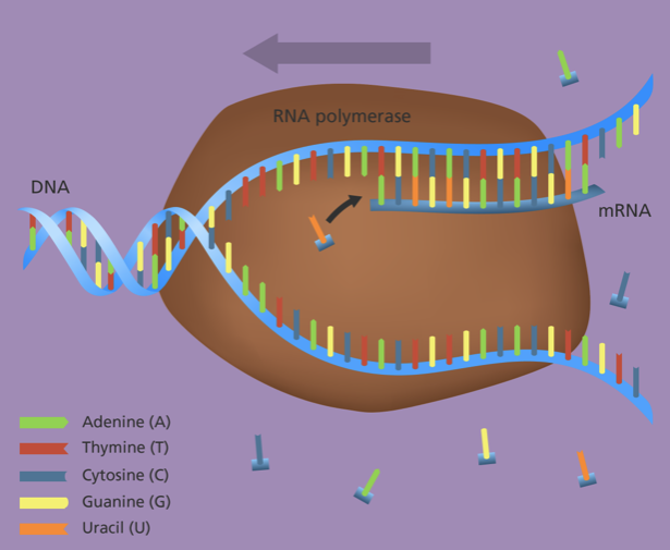
Figure 2.1: Process of transcription borrowed from “Genome Research Limited

"

[ZR20] describes that an evolutionary process in which somatic (non-multiplicative cells, so neither ovule, sperm) mutations that accumulate in a population of tumor cells result in cancer development. Copy number aberrations (CNAs), which are the deletion or amplification of large genomic regions, are a type of somatic mutation common to many types of cancer, including breast cancer. CNAs are classified into multiple types and can cover a broad range of sizes, from thousands of kilobases to entire chromosomes and even chromosome arms. A critical role played by CNAs is in driving the development of cancer, and thus the characterization of these events is crucial in the diagnosis, prognosis and treatment of diseases. Furthermore, CNAs act as an important point of reference for reconstructing the evolution of tumors. Although somatic CNAs are the dominant feature discovered in sporadic breast cancer cases, the elucidation of driving events in tumorigenesis is hampered by the large variety of random, non-pathogenic passenger alterations and copy number variants.

METABRIC consists of 1980 breast-cancer patients split in groups based on two immunohistochemistry sub-types, ER+ and ER-, 6 intrinsic gene-expression subtypes (PAM50) [PPK⁺], 10 Integrative Clusters (IC10)[CSC⁺12], and two groups based on Distance Relapse (the cancer metastasised to another organ after initial treatment or not).

The dataset which we are going to use is the one already pre-processed by [SBT⁺19], because the is already split in five-fold cross evaluation, for each labels class, in order to obtain proportional number of object which same class allover the folds. CNA modality has been processed as well, for it’s feature to come from a Bernoulli distribution, and the clinical data has been filtered through one-hot-encoding process.

2.2 Synthetic Dataset

When developing novel models on top of complex datasets such as METABRIC, it is hard to segregate the source of any errors or results that fail to meet expectations due to the multitude of stages in the learning pipeline: the data integration and graph building cycle, the model training or the classification task. Thus, we will leverage a testing methodology popular in literature to help us point out any errors or inconsistencies, either from a data, architecture design or implementation perspective. Specifically, we will generate a synthetic dataset coming from a Gaussian distribution; this is advantageous because edges can be predefined based on the labels of the artificial data points, and we are also in control of dataset characteristics such as homophily levels.

The requirements of this synthetic dataset are enumerated below along with the design decisions behind them:

1. The dataset will contain objects from two classes as we want to perform a classification task in the final stage to assess the quality of our lower-latent space embeddings

2. To perform data integration, the objects will be described by two modalities, where each modality is sampled from a different normal distribution

3. The distributions used to generate the modality data must be intractable for a Principal Component Analysis i.e. there must be no clear separation of classes after appying PCA, such as in Figure 2.2 (a), because having the objects already clustered would defeat the purpose of the experiment

4. To easily build edges between samples of same class (intra-class) and samples belonging to different classes (inter-class) in order to evaluate how various graph building algorithms reflect on the quality of the lower-space embeddings

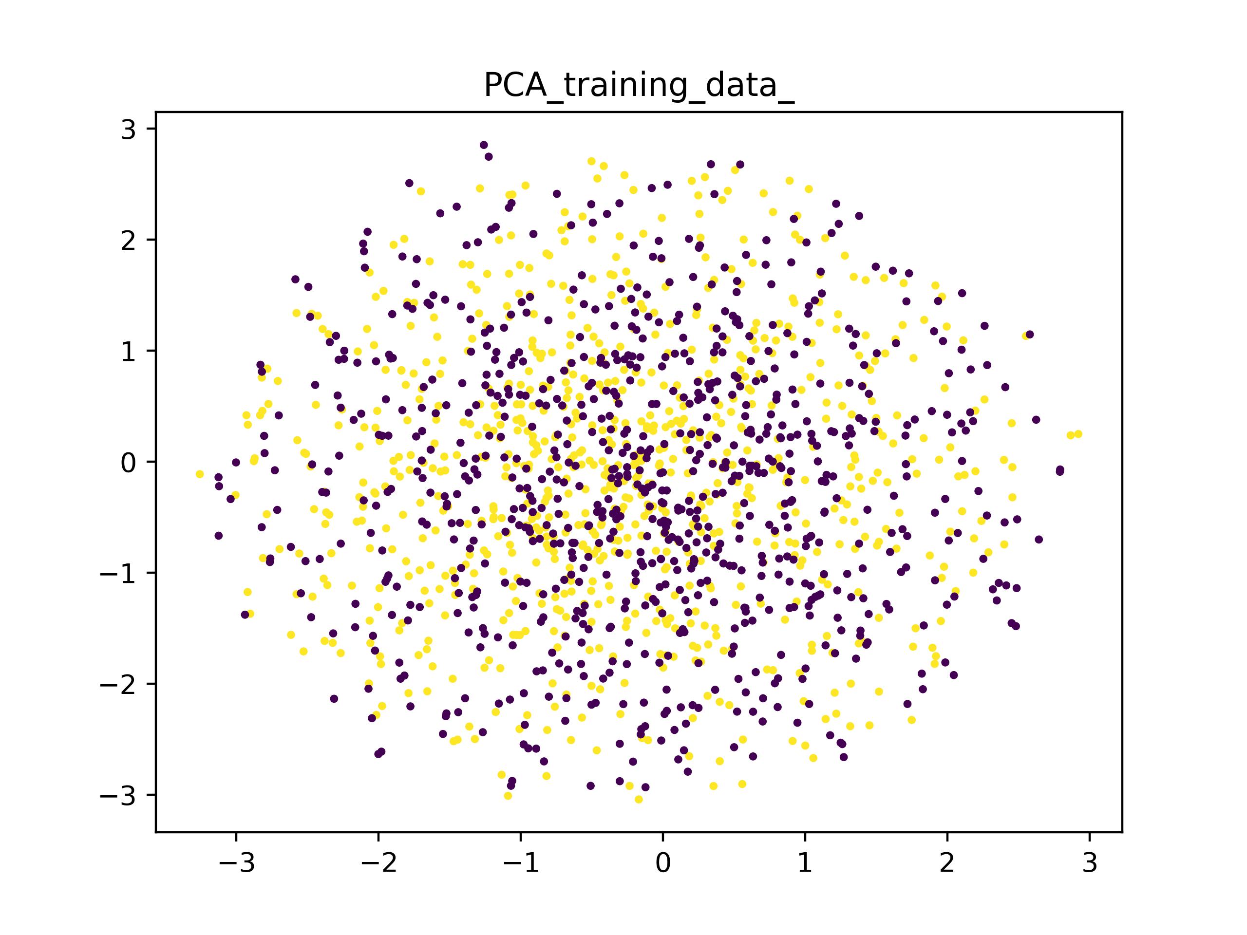
(a)

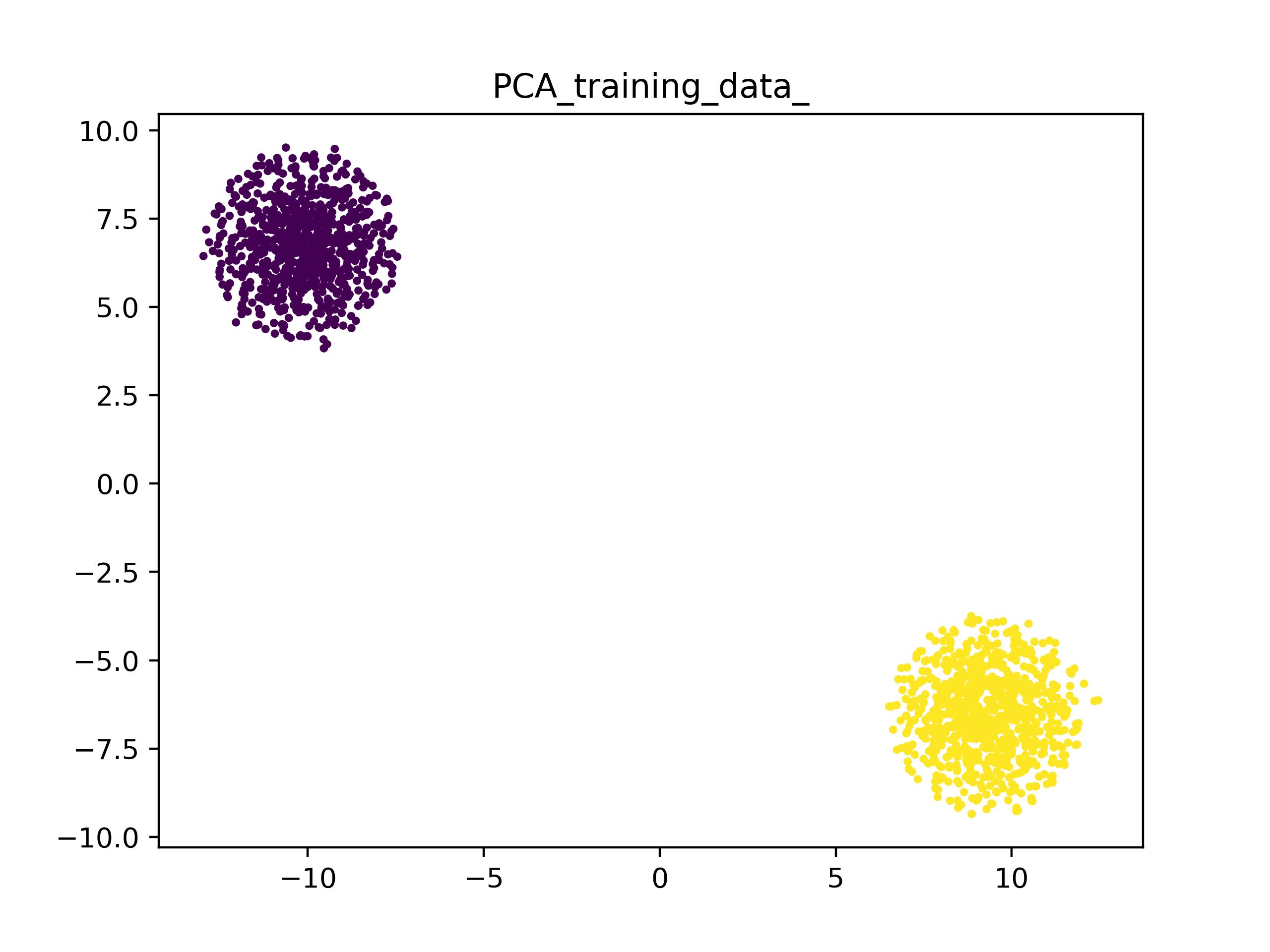
(b)

Figure 2.2: Example of two synthetic datasets, a good one, and a bad one

After considering these matters, we decided that for each class of objects we should sample points with features coming from two multi-Gaussian with high standard deviation, such the feature spaces would overlap with the others class feature space. Let $A$ and $B$ be my two classes of labels. Let $\alpha$ and $\beta$ my two modalities. Now, let’s assume feature space for $\alpha$ has $n$ dimensions, and $\beta$’s feature space has m. Let’s define $\vec{\mu_{\alpha}}$ and $\vec{\mu_{\beta}}$, with $\mu_{\alpha,i}$ and $\mu_{\beta,i}$ are coming from a two uniform distribution with different parameters, that can be freely chosen. We will define $\vec{\mu}_{\alpha,A}=\vec{\mu}_{\alpha}-\theta_{\alpha}$, where $\theta_{\alpha}$ can be again chosen by as, and $\vec{\mu}_{\alpha,B}=\vec{\mu}_{\alpha}+\theta_{\alpha}$. For the second modality the process is similar, by replacing $\alpha$ with $\beta$.

Now we sample $X_{\alpha,A}$ from $\mathcal{N}(\vec{\mu}_{\alpha,A},\vec{\sigma})$, $X_{\beta,A}$ from $\mathcal{N}(\vec{\mu}_{\beta,A},\vec{\sigma})$, $X_{\alpha,B}$ from $\mathcal{N}(\vec{\mu}_{\alpha,B},\vec{\sigma})$ and $X_{\beta,B}$ from $\mathcal{N}(\vec{\mu}_{\beta,B},\vec{\sigma}))$ where $\vec{\sigma}$ is big enough to cause overlap between each modalities feature space. For example, in Figure (a) we have good choice of $\vec{\sigma}$, but in Figure (b) we cannot say the same thing anymore.

2.3 Synthetic Graph

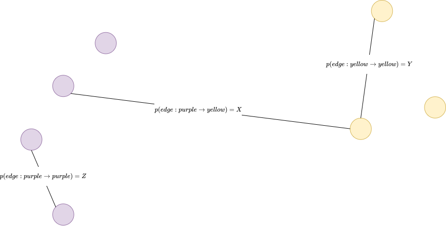
Figure 2.3: Building a graph from the synthetic dataset

In order to build node relations between the data points coming from the Synthetic dataset, we decided to implement a statistical approach over the task. Let purple and yellow be the two possible labels. Our interest was to manipulate graph configurations in such a manner that we would be in control of the number of the edges between nodes with same label and with opposite label. And this is important for many reasons, we will latter explain, but for now the reader must just trust that the performance of the models applied over the dataset will be heavily influenced by this fact. As you can see in 2.3, we will build edges between two purple nodes with probability $Z$, between purple and yellow with probability $X$, and between yellow nodes with probability $Y$. In the experiments and evaluation section we wanted to show of how model’s performance can be influenced by different graphs structures.

While, it might seem a counter-intuitive to build edges this way, it can be rationalized in the following way: if $p(edge:purple\to purple)=1/2$ and $p(edge:yellow\to yellow)=1/2$ then the $p(edge:purple\to yellow)=0$ (we would get two isolated graphs), or if $p(edge:purple\to purple)=1/3$ and $p(edge:yellow\to yellow)=1/3$ then the $p(edge:purple\to yellow)=1/3$. This is the probabilistic approach.

As we mentioned we will used a statistical approach which works the other way around. We will generate random samples of edges between purple-to-purple, purple-to-yellow, yellow-to-yellow nodes and this their number will be x, y , and y. In order to get back to the probabilistic approach, we need to compute $X=\frac{x}{x+y+z}$, $Y=\frac{y}{x+y+z}$, and $Z=\frac{z}{x+y+z}$. If we want to obtain $p(edge:purple\to purple)=1/2$ and $p(edge:yellow\to yellow)=1/2$ then the $p(edge:purple\to yellow)=0$ probabilities, we will just generate for example, $2000$ edges between purple-to-purple nodes and $2000$ edges between yellow-to-yellow nodes. Our decision to build graphs this way, will make further explained in the chapter Graph Neural Networks for Cancer Data Integration.

Chapter 3 Deep Neural Networks

This chapter provides a summary of the most prominent neural network architectures, their potent variants and applicability. We will first introduce the multi-layer perception as a knowledge base for the following models leveraged in this work: Variational Autoencoders (VAE), and Graph Neural Networks (GNN).

In the experiments detailed further in the paper these models have been used in an unsupervised fashion: rather than carrying out regression or classification tasks, the goal is to generate lower-latent space representations of the unlabeled data points. The Variational Autoencoder is at the core of the implemented models, and the convolutional layers are deeply explained as they come up in the graph learning techniques based on order-invariant convolutions. Finally, we introduce GNNs and describe the main approaches to performing unsupervised learning to generate lower-space embeddings of data points: Deep Graph Infomax, which maximizes mutual local information, and Variational Graph Autoencoder, which builds up from the traditional Variational Autoencoder with the addition that the decoder reconstructs the adjacency matrix.

3.1 Multilayer Perceptron

Neural networks are Machine Learning models composed of simple processing units that can compute linear or nonlinear transformations (based on the activation function used) on vector inputs; these processing units are called perceptrons. One perceptron receives a vector $\vec{x}\in\mathbf{R^{n}}$, on which it applies a linear combination by multiplying with a weight vector $\vec{w}\in\mathbf{R^{n}}$ and adding a bias value $b$. Afterwards, a nonlinear function $\sigma$ can be applied to the result to obtain the final value for an output, $y$. The are a multitude of activation functions which are chosen based on the learning task.

$$y=\sigma\left(b+\sum_{i=1}^{n}w_{i}x_{i}\right)=\sigma\left(b+\vec{w}^{T}\vec{x}\right)$$

Multilayer perceptron neural networks are formed of layers of perceptron units which receive inputs from previous layers, and apply the linear combination and activation functions described above to return the output values. For each individual layer, we can compute the output values with the matrix form as follows:

$$\vec{y}=\sigma\left(W\vec{x}+\vec{b}\right)$$ (3.1)

For a two layered perceptron neural network the formula is similar. On top of the $\vec{y}$ obtained in (2.1), we apply another linear transformation by multiplying with the second layer’s weight matrix, adding its bias value and, finally, computing the same or a different activation function. The new result is:

$$\vec{y}=\sigma\left(W\vec{y}_{previous}+\vec{b}\right)=\sigma\left(W\sigma_{previous}\left(W_{previous}\vec{x}+\vec{b}_{previous}\right)+\vec{b}\right)$$ (3.2)

Networks with more than one intermediate layer are called deep neural networks. A natural question that comes with such networks is: "How many layers?". It is argued by Cybenko in [Cyb89] that any bounded continous real function can be approximated with only one layer and a sigmoidal activation layer. However, if this were the truth this chapter would end here, which is not case. There is no perfect architecture and finding a neural network that works for a specific kind of data is an engineering task where a lot of experiments and searching needs to be carried out, in order to find what works better.

3.2 Autoencoders

Generally, an autoencoder is a model that consists of two networks: the encoder, which constructs lower-latent space embeddings from the data points, and the decoder, which reconstructs the input data. The encoder function $E(\dot{)}$ takes $\theta$ as parameter, and the decoder function $D(\dot{)}$ takes $\phi$ as parameter. The lower-space embedding is learned from $E_{\theta}(x)$ and the reconstructed input is $y=D_{\phi}(E_{\theta}(x))$. The two parameters are learned together on the reconstructed data through a loss function chosen upon the underlying data, named reconstruction loss, which is Binary Cross Entropy (BCE) for categorical data, or Mean Square Error (MSE) for continuous data.

$$L_{MSE}(\theta,\phi)=\frac{1}{n}\sum_{i=1}^{n}(x_{i}-D_{\phi}(E_{\theta}(x_{i}))^{2}$$ (3.3)

Let m be the number of classes, then we have:

$$L_{BCE}(\theta,\phi)=\frac{1}{n}\sum_{i=1}^{n}\sum_{j}^{m}x_{ij}log(D_{\phi}(E_{\theta}(x_{i}))$$ (3.4)

Many variants of autoencoders have been proposed to overcome the shortcomings of simple autoencoders: poor generalization, disentanglement, and modification to sequence input models. Among these models are the Denoising Autoencoder (DAE) [VLBM08], which randomly filters-out some of the input features to learn the defining characteristics of the input object; Sparse Autoencoder (SAE) [CNL11] adds a regularization term to the loss function to restrict the lower-latent representations from being sparse (i.e. many zero-valued entries in the feature vectors). Finally, Variational Autoencoder (VAE) [KW13] is presented in the next section.

3.2.1 Variational Autoencoders

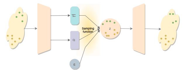
Figure 3.1: Generate low-dimensional representation of the input, regularize it in a Multi-Gaussian distribution, and attempt reconstruction of the original input

Typically, VAE assumes that latent variables to be a centered isotropic multivariate Gaussian $p_{\phi}(z)=\mathbf{N}(z;0,I)$, and $p_{\theta}(z|x)$ a multivariate Gaussian with parameters approximated by using a fully connected neural network. Since the true posterior $p_{\theta}(z|x)$ is untractable, we assume it takes the form of a Gaussian distribution with an approximately diagonal covariance. This allows the variational inference to approximate the true posterior, thus becoming an optimisation problem. In this case, the variational approximate posterior will also take a Gaussian with diagonal covariance structure:

$$q_{\phi}(z|x_{i})=\mathbf{N}(z;\mu_{i},\sigma_{i}I)$$

where $\mu$ and $\sigma$ will be outputs of the encoder. Since both $p_{\theta}(z)$ and $q_{\phi}(z|x_{i})$ are Gaussian, we can compute the discrepancy between the two:

$$l_{i}(\theta,\phi)=-E_{q_{\phi}(z|x_{i})}[logp_{\theta}(x|Z)]+KL(q_{\phi}(z|x_{i})||p_{\theta}(z))$$ (3.5)

with

$$KL(P(x)||Q(x))=P(x)log\left(\frac{P(x)}{Q(x)}\right)$$ (3.6)

The first part of the loss function represents the reconstruction loss i.e. how different is the decoder output from the initial input, and the second part represents the reparametrisation loss. We used both Kullback-Leiber (KL) divergence (reconstruction loss which is used in the original paper describing Variational Autoencoders) and Maximum Mean Discrepancy (MMD) (which has been proved to give better by [SBT⁺19]), which will be employed as an alternative to the KL divergence. While KL restricts the latent space embedding to reside within a centered isotropic multivariate Gaussian distribution, MDD is based on same principle, but uses the fact that two distributions are identical if, and only if, their moments are identical, with:

$$MMD(P(x)||Q(x))=E_{p(x),p(x^{\prime})}[k(x,x^{\prime})]+E_{q(x),q(x^{\prime})}[k(x,x^{\prime})]-2E_{q(x),q(x^{\prime})}[k(x,x^{\prime})]$$ (3.7)

where $k(x,x^{\prime})$ denotes the Gaussian kernel with $k(x,x^{\prime})=e^{-\frac{||z-z^{\prime}||^{2}}{2\sigma^{2}}}$.

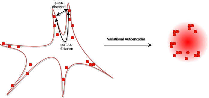
Figure 3.2: Although two points on the initial manifold might be close to each other space-wise, the distance on the actual surface might actually be larger, so a multivariate Gaussian representation of the data will ’flatten’ the manifold’s surface to better represent the similarity or disparity of the points. This is an intuitive picture.

3.3 Convolutional layers

Datasets can take a plethora of shapes and forms as particular data sources are better described by different modalities, ranging from graphical and textual, to physiological signals and many other biomedical formats. Hence, the way we infer outcomes or define functions to describe the data must be adapted to the underlying characteristics of the dataset. For example, in most visual examples it is important to note that an area of neighbouring points present similar features, and leveraging this information helps in building a better performing model than just analysing all points in separation. This builds the case for convolutional layers that can summarise and learn functions for neighbourhoods of points, which is better suited for image-based datasets than multilayer perceptrons. Visual data generally has an $h\times w\times d$ shape where $h$ is the height, $w$ the weight, and $d$ the number of channels (e.g. colour images have three channels, RGB).

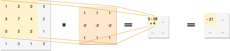
Figure 3.3: Convolutional layer applied on a single-channel data point

Let $X\in\mathbf{R}^{h\times w}$ and a kernel matrix $K\in\mathbf{R}^{n\times m}$ (ex. $m=n=3$). The new image $X^{\prime}$ has the following formula:

$$X_{ab}^{\prime}=\sum_{i=1}^{n}\sum_{j=1}^{m}K_{ij}X_{a+i-1,b+j-1}$$

3.4 Graph Neural Network

This section presents Graph Neural Networks (or Graph Convolutional Networks, based on the source of the [BG17], [BZSL13], [DBV16]), which are learning techniques dealing with graph structured data that build intermediate feature representations, $\vec{x}^{\prime}_{i}$, for each node i.

What must be noted is that all the architectures mentioned can be reformulated as an instance of message-passing neural networks [KW16a].

3.4.1 Graph Convolutional Layer

Convolutional layers were introduced because most graph neural networks adopt the convolutional element of it. Intuitively, when dealing with graph-like data we can say that nodes being neighbours with each other should be significant for the way we try to learn lower space embeddings. In our graph-shaped data, filters are applied to patches of neighbourhoods just as in CNN’s example. These filters that we apply need to be order invariant because by taking the immediate neighbourhood of a node we cannot define a precise order of the neighbour nodes.

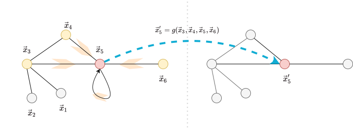
Figure 3.4: Convolutional layer applied on a single-node

Let $\mathcal{G}=(\mathcal{V},\mathcal{E},X)$ a graph where $\mathcal{V}$ is the vertex set, $\mathcal{E}$ is the set of edges, and X is the feature matrix, each row describing the features of vertex i from $\mathcal{V}$. From $\mathcal{E}$ we can build $A$, the adjacency matrix, with following the rule: if $(i,j)\in\mathcal{E}$, then $A_{ij}=1$ else $A_{ij}=0$. A simple way to aggregate is to multiply X, the node feature matrix, with A.

$$X^{\prime}=\sigma(AXW)$$ (3.8)

where W is a parametrized learnable linear-transformation, shared by all nodes, and $\sigma$ is a non-linearity, an activation function. A problem with this exact shape of the function is that after passing our inputs through it, we lose for each node it’s own features, because $A_{ii}=0$, as $(i,i)\notin\mathcal{E}$. A simple solution to this is to write $A^{\prime}=A+I_{n}$ where $n=|\mathcal{V}|$. And now we have:

$$X^{\prime}=\sigma(A^{\prime}XW)$$ (3.9)

Because $A^{\prime}$ may modify the scale of the output features, a normalisation is needed. So we define $D$ with $D^{\prime}_{ii}=\sum_{j}A^{\prime}_{ij}$, returning the degree matrix,

$$X^{\prime}=\sigma(D^{\prime-1}A^{\prime}XW)$$ (3.10)

Node-wise, the same equation can be rewritten as below, which resembles mean-pooling from CNNs:

$$\vec{x}^{\prime}_{i}=\sigma(\sum_{j\in N_{i}}\frac{1}{|N_{i}|}W\vec{x}^{\prime}_{j})$$ (3.11)

By using symmetric-normalisation we get to the GCN update rule:

$$X^{\prime}=\sigma(D^{\prime-\frac{1}{2}}A^{\prime}D^{\prime-\frac{1}{2}}XW)$$ (3.12)

Which node-wise has following equation:

$$\vec{x}^{\prime}_{i}=\sigma(\sum_{j\in N_{i}}\frac{1}{\sqrt{|N_{i}||N_{j}|}}W\vec{x}^{\prime}_{j})$$ (3.13)

3.4.2 Variational Graph Autoencoder

Variational Graph Autoencoders and Graph Autoencoders were demonstrated by [KW16b] to learn meaningful latent representation on a link prediction task on popular citation network datasets such as Cora, Citeseer, and Pubmed.

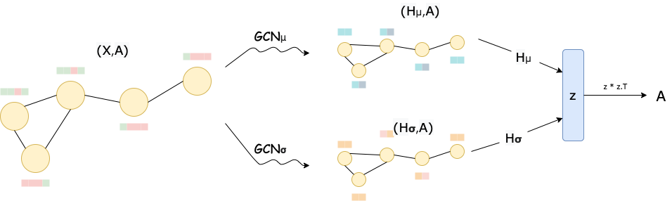
Figure 3.5: Convolutional layer applied on a single-channel point

Let $\mathcal{G}=(\mathcal{V},\mathcal{\epsilon})$ an undirected and unweighted graph with $N=|\mathcal{V}|$ nodes. Let $\mathbf{A}$ be the adjacency matrix of $\mathcal{G}$. Node features are summarized in the vector $X\in\mathbf{R}^{N\times F}$, and $\mathbf{D}$ is the degree matrix. The authors further introduce the stochastic latent variables $\mathbf{z}_{i}$, summarized in $\mathbf{R}^{N\times F^{\prime}}$

Similar to the Variational Autoencoder, a mean vector and logarithmic variation vector are produced, with two Encoder functions which can be composed by Graph Convolutional Layers, and then, by using a sampling function, the stochastic latent variables are reproduced. The loss function used for this learning task is exactly the same as the one used for a variational autoencoder, with the difference that for the reconstruction, the authors use inner dot product of the latent variables and compare the output with the input adjacency matrix.

$$\mathcal{L}=\mathbf{E}_{q(Z|X,Z)}[log_{p}(A|Z)]-KL(q(Z|X,A)||p(Z))$$ (3.14)

As Z has $N\times F^{\prime}$ dimension, we notice that $Z\cdot Z.T$ will have $N\times N$ size, so it is possible to apply a loss function on $Z\cdot Z.T$ and adjacency matrix.

3.4.3 Deep Graph Infomax

Deep Graph Infomax was first described by Velickovic in [VFH⁺19]. The approach is based on maximizing local mutual information, and was inspired from [HFLM⁺18] Deep Infomax.

For a generic graph-based unsupervised Machine Learning task setup, we will use the following notations. Let $X=\{\vec{x_{1}},\vec{x_{2}},...\vec{x_{n}}\}$ be node feature set, where N is the number of nodes in our graph. Let $A\in\mathbf{R^{N\times N}}$ be the adjacency matrix with $A_{i,j}=1$ if and only if there is an edge between node i and j. The objective is to learn an encoder, $\epsilon:\mathbf{R^{N\times F}}\times\mathbf{R^{N\times N}}\to\mathbf{R^{N\times F^{\prime}}}$, such that $\epsilon(X,A)=H=\{\vec{h_{1}},\vec{h_{2}},...\vec{h_{n}}\},$ The representations can be latter used for a classification task, and this will also represent a way we can evaluate the quality of our embeddings.

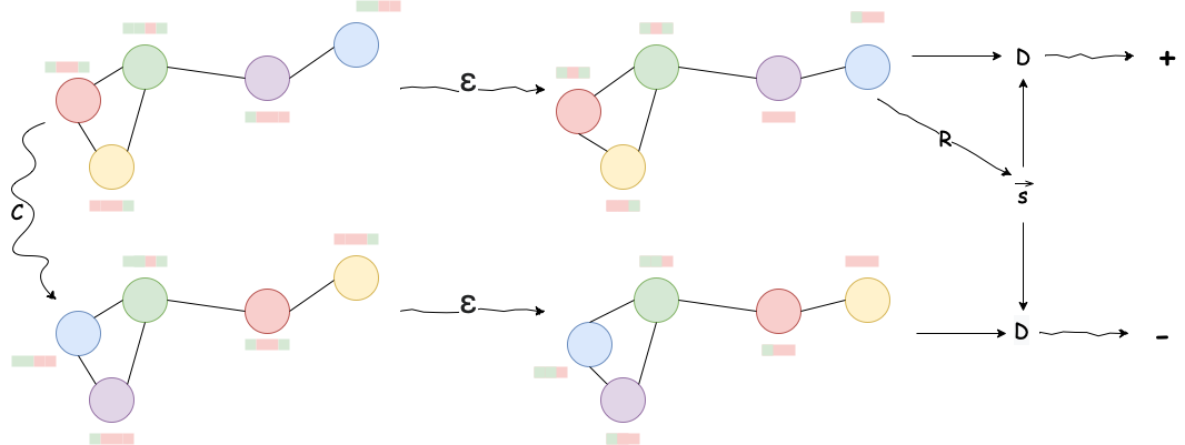
Figure 3.6: High-level overview of Deep Graph Infomax

In order to obtain graph-level summary vectors, $\vec{s}$, the authors leverage a readout function $R:\mathbf{R}^{N\times F}\to\mathbf{R}^{F}$ to summarise the obtained patch representation into a graph-level representation, $\vec{s}=R(\epsilon(X))$. For maximizing the local mutual information, $\mathit{D}:\mathbf{R}^{F}\times\mathbf{R}^{F}\to\mathbf{R}$, the discriminator is deployed. $\mathit{D(\vec{h_{i},\vec{s}})}$ should score higher if the patch representation is found in the summary.

The negative samples for D, are computed with a corruption function $\mathit{C}:\mathbf{R}^{N\times F}\times\mathbf{R}^{N\times N}\to\mathbf{R}^{M\times F}\times\mathbf{R}^{N\times N}$. The choice of the corruption function governs the specific kind of information that will be maximized. In my case, I have solely used a simple shuffling of the nodes features, letting the edges to stay in place. $(\tilde{X},\tilde{A})=\mathit{C}(X,A)=(X_{shuffled},A)$ for this precise case.

The authors followed the original paper, which was not concerned with graph shaped like data [HFLM⁺18], and use a noise-constrastive type object with with a standard binary cross entropy loss between the samples from the joint and product of the marginals.

$$\mathit{L}=\frac{1}{N+M}\left(\sum_{i=1}^{N}\mathbf{E}_{(X,A)}\left[log\mathit{D}\left(\vec{h}_{i},\vec{s}\right)\right]+\sum_{j=1}^{M}\mathbf{E}_{(\tilde{X},\tilde{A})}\left[log\left(1-\mathit{D}\left(\vec{h}_{i},\vec{s}\right)\right]\right)\right)$$ (3.15)

Chapter 4 Recreating Two State-of-the-Art Models

4.1 Description of Models

The authors in “Variational Autoencoders for Cancer Data Integration: Design Principles and Computational Practice" [SBT⁺19] use several variational autoencoder architectures to integrate the METABRIC subsets containing CNA, mRNA and clinical data; the approaches in the paper are evaluated by combining pairs of modalities. We reproduce two models from this work, specifically CNC-VAE (Concatenation Variational Autoencoder) and H-VAE (Hierarchical Variational Autoencoder), both based on the VAE architecture. The difference between the two designs is where in the model the data integration is performed, with CNC-VAE concatenating the input features at the earliest stage, and H-VAE using hierarchical ordering, i.e. lower-latent space representations will be learned for each modality in part by a separate lower-level VAE, after which another higher-level VAE is applied on concatenation of the previously learned representations.

Generally, the integrative models obtain higher results than the raw data with CNC-VAE obtaining accuracies as high as 82% on PAM50 with an SVM classifier. X-VAE obtains good results on DR (77%), and IC10 (85%), while H-VAE obtains accuracies from DR (77%) and PAM50 (82%).

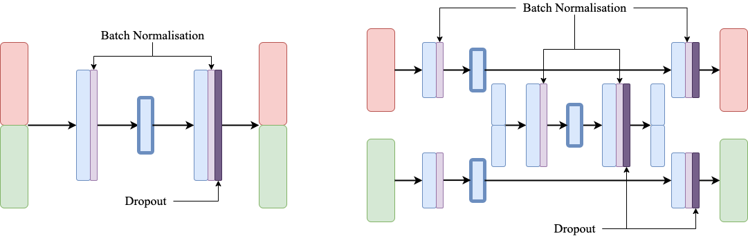
Figure 4.1: CNC-VAE and H-VAE. The two feature matrices are represented with red and green.

For CNC-VAE, the feature matrices of the inputs are concatenated and then fed to a Variational Autoencoder. The model is employed as a benchmark and as a proof-of-principle by the authors for learning a homogeneous representations from heterogeneous data sources. Even though early concatenation is prone to cause more noise, and modalities with lower-dimensional feature spaces will carry a weaker weight compared to the higher-latent feature vectors, this approach obtains competitive results (up to 84%) with the other architectures. While the complexity of this simple architecture lies in the highly domain-specific data preprocessing, utilising a single objective function of combined heterogeneous inputs might not be ideal in other settings.

Unlike CNC-VAE, H-VAE learns lower-latent representations for all heterogeneous sources independently, and then concatenates the resulting homogeneous representations. The learning process takes place by training a lower-level Variational Autoencoder on each separate modality. After training these autoencoders, we concatenate the resulting lower-space embeddings for all modalities, and then train a higher-level Variational Autoencoder to learn the summarised embeddings of all intermediate representations. While for CNC-VAE we need to train only one network, for H-VAE we are going to train N + 1 neural networks, where N is the number of modalities.

Both models use Batch Normalization (light violet) and Dropout(0.2) (dark violet) layers which are marked in Figure 4.1. Dense layers use ELU activation function, with the exception of last dense layer which can also use according to case sigmoid activation(when the integration task is for CNA+Clin, categorical data). Where possible the reconstruction loss, is Binary Cross Entropy if data is categorical, and Mean Squared Error if data is continuous. For reparametrisation loss I have chosen MMD, because it gave significantly better results for the authors. Among the hyper-parameters we have the dense layer size $ds$, the latent layer size $ds$, and $\beta$ the weight balancing between the reconstruction loss and the reparametrisation loss.

$$\mathcal{L}=\mathcal{L}_{Reconstruction}+\beta\times\mathcal{L}_{Reparametrisation}$$

As an optimizer, all models use Adam with a learning rate of $0.001$

4.2 Evaluation and results

The environment in which I chose to reproduce CNC-VAE and H-VAE coming from [SBT⁺19] is PyThorch [PGM⁺19], the originating one being TensorFlow with Keras [AAB⁺16]. I encountered a few challenges in the process of translating the models since some of the libraries in Tensorflow with Keras were outdated. Also, in the original code, the correct version of the H-VAE model was located in a different folder than the other models.

The method of evaluation used is 5-fold cross validation. Each class of folds corresponding to a class of labels, being stratified, so making sure the distribution of labels over the folds is uniform.

4.2.1 Hyper-parameter analysis

For evaluating the quality of the reproduced models we carry out two experiments. The first one is performed to understand what hyper-parameter settings would be optional for each modality and each label, which is also the testing approach followed by the recreated paper [SBT⁺19]. As we wanted to avoid repetition of results, the hyper-parameter search was done on Clin+CNA and DR (distance relapse) label. As noted by the authors, Naive Bayes classifier does not have any parameters, so it would be a good choice as the classifier used on top of our lower-space representations.

For my hyper-parameter setting I have picked $ds\in\{128,256,512\}$, $ls\in\{32,64\}$, and $\beta\in\{1,25,50,100\}$. The results can be seen in Figures 4.2 and 4.3.

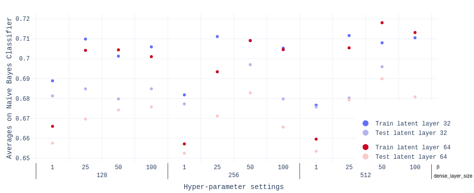
Figure 4.2: CNC-VAE performance with different hyper parameters settings.

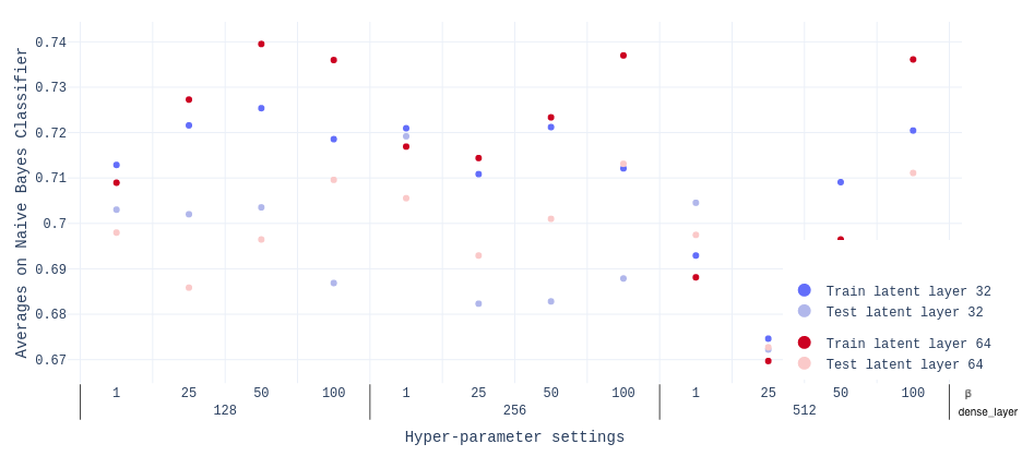
Figure 4.3: H-VAE performance with different hyper parameters settings.

4.2.2 Best model assessment

For the final experiment, we have picked fixed vales for ls, ds, $\beta$, and compared the accuracies of three classifiers: Naive Bayes, Support Vector Machine, and Random Forest, applied on the latent-lower space representations produced by H-VAE, and CNC-VAE. Because for $ls=32$, $ds=128$, $\beta=25$ the results where generally good, I ran both my models with these parameters, and obtained the results in Table 4.1. Generally, the results obtained in the original paper are better, but it must be noted that the aim of the authors was to fine-tune their models, while my goal was to show that I am able to reproduce models, and obtaining competitive results with the original ones. Another likely factor might is the difference in the learning time for H-VAE, which uses three different autoencoder networks. In our experiments, we allowed 150 epochs for each network.

		CNC-VAE			H-VAE
		CNA + mRNA	Clin + mRNA	Clin + CNA	CNA + mRNA	Clin + mRNA	Clin + CNA
ER	NB	90	92	85	87	89	81
	SVM	93	94	88	92	92	85
	RF	88	90	83	87	88	80
DR	NB	66	69	70	67	68	70
	SVM	68	71	70	62	69	72
	RF	67	69	56	67	69	69
PAM50	NB	63	67	55	60	65	51
	SVM	68	73	59	67	72	54
	RF	62	67	54	57	58	47
IC	NB	68	74	59	66	62	53
	SVM	75	79	63	73	73	56
	RF	63	64	55	58	53	45

Table 4.1: Test results for classification with Naive Bayes (NB), Suport Vector Machine (SVM), and Random Forest (RF) of lower-latent representations produced by CNC-VAE and H-VAE, in percentages (%).

Finally, we will discuss the contrast between the results we obtained and those in the original paper [SBT⁺19]. Although we carried out our own hyper-parameter search on the same architectures, we arrived at a different setting that obtained better results on a small subset of modality and label class combinations but generally performed worse. Secondly, the implementation of our project was written in PyTorch, while the underlying Machine Learning framework leveraged in the reference paper was Tensorflow with Keras. Even though both frameworks overlap in supported functionalities overall, there are several methods that exist in Tensorflow but not in Pytorch, and custom implementations often have a minor impact on the model training. One of the main differences is training in batches, which comes out of the box with TensorFlow, but had to be manually implemented in PyTorch in our experiments. Another potential issue is the implementation of Maximum Discrepancy Loss function in PyTorch, because the variants found in other publications were different from the one written in TensorFlow, which was not directly transferable in PyTorch.

For fixed hyper-parameters, there is a total of $5(folds)\times 3(modalities)\times 4(labels)=60$ models to train. For the hyper-parameters sets that the reference paper proposes and the two models, we would need to train $60\times 108=6480$ different models. A model trains in cca. 2 minutes. That would be approximately 300 hours, which is 12 whole days to get best hyper-parameter settings for the two models. Thus, we only trained on a single fold to reduce the training time by five. For the best hyper-parameter setting we found, CNC-VAE clearly out-performs H-VAE.

Chapter 5 Graph Neural Networks for Cancer Data Integration

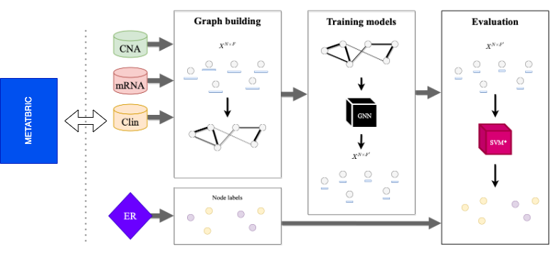
Figure 5.1: This chapter is split in three modules: Graph Construction, Introducing novel Unsupervised Integrative Graph Neural Network, and Evaluate the quality of the lower latent space representations.

This chapter presents the approaches used to generate lower-dimensional representations for multiple integrated modalities. We will first introduce the graph construction algorithms along with the advantages and downsides, followed by the proposed integrative unsupervised models. Finally, we are evaluating the quality of the obtained lower-space representation.

The data sets employed for graph construction are METABRIC and the synthetic dataset described earlier. The synthetic data will be used to discover the best settings for the proposed Graph Neural Networks and to demonstrate the functionality of the proposed models. Furthermore, METABRIC will be leveraged in hyper-parameter fine-tuning for the graph construction modules thanks to the varied distribution of the four classes of labels (ER, DR, PAM, IC).

Finally, we will present best results obtained by the proposed models for each class of labels and then discuss conclusions in the final chapter.

5.1 Graph Construction Algorithms

Graph Neural Networks require the input data to conform to a graph shape i.e. to have a matrix of features, $X$, containing all node information, and a matrix of adjacency, $A$. Since METABRIC does not store the relationship between patients , we need to define a module that builds graphs from feature matrix, X. The quality of the resulting graph will influence the final results - we will describe what graph quality is in a quantitative manner over the next sections, but to give the reader an initial intuition, the following question can be posed: “Should nodes with the same or different labels be connected by edges?".

5.1.1 From feature matrix to graph

Assume a feature matrix $X\in\mathbf{R}^{N\times F}$, for which N is the number of objects and F is the number of features which define the space coordinates of the samples. To transition from a static data set to a graph, one needs to “draw" edges between the objects, which will in turn be visualised as nodes. One naive but working solution is to link data points if they are “close" to each other, where the metric describing closeness is the Euclidean distance. Assume a and b are the coordinates of two points A and B from X

$$dist_{Euclidian}(A,B)=\sqrt{a^{2}-b^{2}}$$

In specialised literature, the most popular ways to connect points in space that rely on Euclidean distance are:

• Use a radius, $r$, as a threshold, and trace edges between nodes if the Euclidean distance between them is lower than $r$.

• Use the K-Nearest Neighbours (KNN) method, which for a node A will return the $k$ nearest neighbours based on the Euclidean distance between nodes.

• Employ a combination of the two approaches presented above for different values of $k$ and $r$.

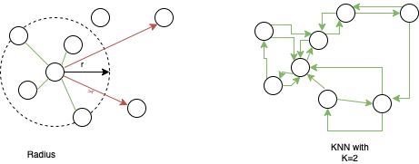
Figure 5.2: Graphic representation for choosing a threshold, $r$, for the radius method, or $k$ for KNN and the results of applying the two methods in separation

Furthermore, to objectively assess the quality of the graphs presented in the next sections, we will introduce a metric cited by multiple sources in literature, namely homophily. Intuitively, it is employed to analyze the ratio of nodes connected by edges that have the same label.

5.1.2 Quantifying the quality of a graph

Homophily is a metric that has been defined in many ways by different papers: edge homophily [ZYZ⁺20], node homophily [PWC⁺20] and edge insensitive [LHL⁺21]. In the context of this project we will refer mainly to edge homophily.

Definition 1

(Edge Homophily) Given a $\mathcal{G}=\{\mathcal{V},\mathcal{E}\}$ and a node label vector $y$, the edge homophily is defined as the ratio of edges that connect nodes with same label. Formally, it is defined as:

$$h(\mathcal{G},{y_{i},i\in\mathcal{V}})=\frac{1}{|\mathcal{E}|}\sum_{(j,k)\in\mathcal{E}}\mathbf{1}(y_{j}=y_{k})$$ (5.1)

where $|\mathcal{E}|$ is the number of edges in the graph and $\mathbf{1}(A=B)$ returns $1$ if $A$ and $B$ have the same label, and $0$ if they do not.

A graph is typically considered homophilous when $h(\cdot)$ is large (typically, $0.5<h(\cdot)<1$), given a suitable label context. Graphs with low edge homophily ratio are considered to be heterophilous.

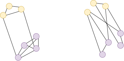
Figure 5.3: Left graph has a higher homophily than the right one, where the ’yellow’ ’purple’ colours represent the labels of the nodes

The works in [AEHPK⁺19], [CPLM21], [CJP⁺18] argue that strong homophily is needed in order to achieve good performances. The next subsection presents an analysis of the homophily levels in different graph construction settings.

5.1.3 Graphs build out of METABRIC modalities

In this section, we analyse how different values for $r$ and $k$ influence the overall homophily levels for each modality in part and all label classes. As previously mentioned, homophily is a metric that measures how labels are distributed over neighbouring nodes (linked through an edge), hence, measure these levels is helpful because it creates an expectation for the lower-dimensional embeddings produced by the GNN. For example, if some related nodes belong to different labels, the lower-latent space representations will not be very accurate for those nodes.

The next sub-sections present the obtained homophily levels over the three modalities for the four classes of labels: ER, DR, PAM and IC. Each patient can be described in terms of ER+ or ER-, positive DR and negative DR, 5 sub-types of breast cancer - PAM, and 10 identified through research clusters - IC.

Homophily levels for each class of labels on: Clinical data, and multi-omic data (mRNA, CNA), by using K Nearest Neighbours

By looking at the tables below, we can learn the following aspects: in the KNN case, the homophily levels don’t vary a a lot, in fact the remain at the same levels over an increase in the number of edges. In the case of the IC class of labels, notice that the results coming from CNA (40%) and Clin (17%) are very low.

[respect all]csv/k/clin.txt

Table 5.1: Homophily of graph build on Clin

[respect all]csv/k/rnanp.txt

Table 5.2: Homophily of graph build on mRNA

[respect all]csv/k/cnanp.txt

Table 5.3: Homophily of graph build on CNA

Homophily levels for each class of labels on: Clinical data, and multi-omic data (mRNA, CNA), by using Radius R

[respect all]csv/r/clin.txt

Table 5.4: Homophily of graph build on Clin

[respect all]csv/r/rnanp.txt

Table 5.5: Homophily of graph build on mRNA

[respect all]csv/r/cnanp.txt

Table 5.6: Homophily of graph build on CNA

By looking at the tables we can learn following aspects. In the Radius case homophily levels vary a lot, sometimes even 40% (in the mRNA $H_{IC}$ case). This means that or choice of R matters a lot. Another aspect that can be noticed is that for good levels (above 70%) of homophily, most of the time that graph conformation will have lots of isolated nodes, fact which can be disastrous for graph neural networks.

Now, with some intuition build on how graphs would behave like, we will reveal to the reader that a combination of the two methods will be used in order to get the most out of both. By using KNN we will ensure that no nodes are isolated, and by using the radius method we will ensure that the clusters of nodes close in space will be related through edges regardless of their number (limitation of the KNN).

The next section will present the proposed 4 models that attempt integration on graph structured data. While the fist two: CNC-VGAE and CNC-DGI attept early integration (by direct concatenation of the featuers), 2G-DGI and Hetero-DGI will attempt mixed integration, by concatenating their lower latent features in the middle of the learning phase.

5.2 Graph Neural Network Models For Data Integration

We researched unsupervised learning approaches and models that could aid in the integration of two feature matrices that describe the same items in different ways for a data integration task. A first strategy would be to concatenate the two feature matrices and construct a graph on top of that, then apply either a Variational Graph Autoencoder or a Deep Graph Infomax. A second technique is to integrate two graphs on which will apply GCN layers, and then use a Dense Layer to ’filter’ the two concatenated feature matrices during the integration phase. A third option is to create a hetero graph and concatenate the upper layer and bottom layer features at some point. Both the second and third method will imply at some point the use of Deep Graph Infomax.

We have selected the Deep Graph Infomax architecture type to integrate two graphs or a hetero graph. This is because for readout and discrimination the only inputs are latent feature vectors, with no adjacency matrix. The adjacency matrix can be very tricky to work with, and we will give two scenarios to prove our point. It is necessary to know that when applying a GCN layer over data points both their feature matrix and their adjacency matrix is needed.

• Consider applying two GCN layers to two graphs in order to integrate them. Then we wish to concatenate the resulted feature matrices and apply another GCN layer. A question is which adjacency matrix should we keep, the one from the first graph or the one from the second graph? Obviously the two graphs have different adjacency matrices.

• Another problem specific to VGAE is that, even if we can get lower-latent variables to incorporate the information from two graphs, when reconstructing, if we only use inner product we can only build one adjacency matrix, since the inner product of the lower latent-variables has no parameters to train. Alternatively, two layers could be added before generating the two adjacency matrices, and then rebuilt with the inner product. However, in the original paper the adjacency matrix is built directly from the latent space with a function that doesn’t have any parameters.

5.2.1 Notation and background knowledge

Let $X_{1}^{N\times F_{1}}$ and $X_{2}^{N\times F_{2}}$ be the two modalities we want to integrate. Let $\mathcal{G}:R^{N\times F_{i}}\to R^{N\times F_{i}}\times R^{|\mathcal{E}_{i}|\times 2}\times R^{|\mathcal{E}_{i}|}$, where $\mathcal{G}$ will return the feature matrix together with the edges set $\mathcal{E}_{i}$, and a list of their attributes.

Each architecture in part, will have a component $Encoder$, this will return the latent lower space representation and will have the following shape, with $ls$ the dimension of the lower latent space:

A graph encoder in this case will represent a function

$$Encoder:\mathbf{R}^{N\times F}\times\mathbf{R}^{|\mathcal{E}|\times 2}\times R^{|\mathcal{E}|}\to\mathbf{R}^{N\times ls}$$

or

$$Encoder:2\times\mathbf{R}^{N\times F_{i}}\times\mathbf{R}^{|\mathcal{E}_{i}|\times 2}\times R^{|\mathcal{E}_{i}|}\to\mathbf{R}^{N\times ls}$$

for the Two Graphs Deep Infomax, which will be present in the next sections.

The encoder will be an ensemble of graph convolutional layers, plus some special integrative layer which will describe depending to case. Even thought there are a lot of current choices for the graph convolutional layers: ChebConv [DBV16], SAGEConv [HYL17], GATConv [VCC⁺17], GCNConv, etc, because it permits for edge attributes, GCNConv has been chosen. The number of layers will represent a parameter, which will be studied in the upcoming sections by varying their number from 1-3, literature mentioning that 3 layers are usually ideal for encoding task [VFH⁺19].

For an edge with size $s$ it’s value of the feature will be $e^{-s}$. This is a good way to write edge features because edges that unite close neighbour points will have values between $1$ and $0.5$ and far apart nodes which will be united will have values bellow $0.1$. This mapping for edges features is also used by Similarity Fusion Network’s paper [WMD⁺14].

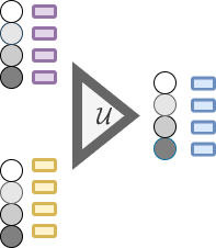
Figure 5.4: $\mathbf{\mathcal{U}}$: Special integration layer

The special integration layer from 5.4 will be defined for each model in part (2G-DGI and Hetero-DGI), and will work differently for each of the two mentioned models.

In order to simplify notation, we will not mention edge attributes in the following subsections, but they will be used in thetraining of the models.

5.2.2 Concatenation Of Features: CNC-DGI and CNC-VGAE

This method of integrating the two datasets is pretty straight forward. Having two feature matrices $X_{1}\in\mathbf{R}^{N\times F_{2}}$ and $X_{2}\in\mathbf{R}^{N\times F_{2}}$, the concatenation of them both would result in a matrix $X_{12}\in\mathbf{R}^{N\times(F_{1}+F_{2})}$. On top of this we apply our building graph method, and then we take our graph through the unsupervised method for getting lower space embeddings of our choice.

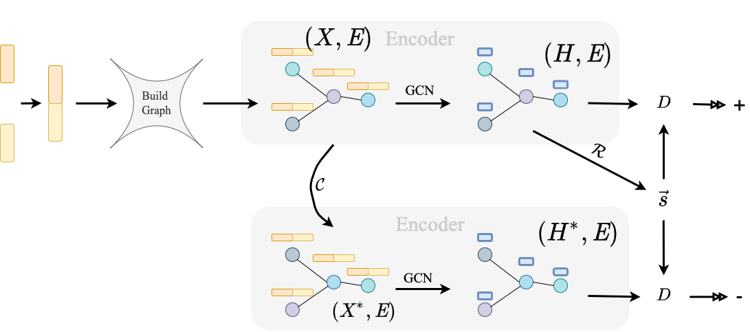
Figure 5.5: CNC-DGI: Apply Variational Autoencoder on top of the graph built on concatenated inputs.

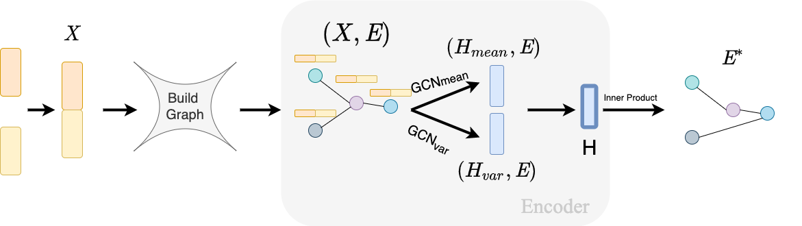
Figure 5.6: CNC-VGAE: Apply Variational Autoencoder on top of the graph built on concatenated inputs

After training, the $\mathit{Encoder}$ from both will return lower-latent space embeddings with shape $\mathbf{R}^{N\times\mathit{ls}}$ where $\mathit{ls}$ is the dimension of the latent space. For 5.5 and 5.6 the encoder will return $H^{N\times\mathit{ls}}$.

5.2.3 Two Graphs: 2G-DGI

Take $X_{1}\in\mathbf{R}^{N\times F_{1}}$ and $X_{2}\in\mathbf{R}^{N\times F_{2}}$ and build two graphs, $\mathcal{G}_{1}=(X_{1}^{N\times F_{1}},\mathit{E}_{1})$ and $\mathcal{G}_{2}=(X_{2}^{N\times F_{2}},\mathit{E}_{2})$. The $GCN_{1}:R^{N\times F_{1}}\to R^{N\times\mathit{ls}}$ and $GCN_{2}:R^{N\times F_{2}}\to R^{N\times\mathit{ls}}$ are different for $\mathcal{G}_{1}$ and for $\mathcal{G}_{2}$ because the nodes have different feature size.

Here the encoder, $\mathit{Encoder}:\mathbf{R}^{N\times F_{1}}\times\mathbf{R}^{N\times F_{2}}\to\mathbf{R}^{N\times\mathit{ls}}$ and

$$\mathit{Encoder}(X_{1},\mathit{E}_{1},X_{2},\mathit{E}_{2})=\mathcal{U}(GCN_{1}(X_{1},\mathit{E}_{1}),GCN_{2}(X_{2},\mathit{E}_{2}))$$

where $\mathcal{U}$ can have for example the following shapes:

$$\mathcal{U}_{Dense}(GCN_{1}(X_{1},\mathit{E}_{1}),GCN_{2}(X_{2},\mathit{E}_{2}))=$$

$$=Dense^{(2\times\mathit{ls}\to\mathit{ls})}((GCN_{1}(X_{1},\mathit{E}_{1})||GCN_{2}(X_{2},\mathit{E}_{2})))=$$

$$=Dense^{(2\times\mathit{ls}\to\mathit{ls})}(H_{1}||H_{2})=H$$ (5.2)

$$\mathcal{U}_{avg}(GCN_{1}(X_{1},\mathit{E}_{1}),GCN_{2}(X_{2},\mathit{E}_{2}))=\frac{GCN_{1}(X_{1},\mathit{E}_{1})+GCN_{2}(X_{2},\mathit{E}_{2})}{2}=\frac{H_{1}+H_{2}}{2}=H$$ (5.3)

One observation worth making is that while $\mathcal{U}_{Dense}$ has parameters, $\mathcal{U}_{Avg}$ does not. We propose those two different special integration layers because we can learn what works better in the DGI context.

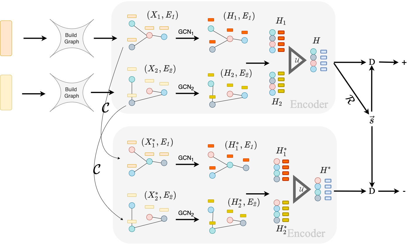
Figure 5.7: 2G-DGI: Two graphs integration

5.2.4 Heterogeneous Graph: Hetero-DGI

In [WJS⁺19] heterogeneous graphs have the following definition:

Definition 2

A heterogeneous graph denoted as $\mathcal{G}=(\mathcal{V},\mathcal{E})$ , consists of an object set $\mathcal{V}$ and a link set $\mathcal{E}$. A heterogeneous graph is also associated with a node type function $\theta:\mathcal{V}\to\mathcal{A}$ and a link type mapping function $\omega:\mathcal{E}\to\mathcal{R}$. $\mathcal{A}$ and $\mathcal{R}$ denote two sets of predefined object types and link types, where $|\mathcal{A}|+|\mathcal{R}|>2$.

Take $X_{1}\in\mathbf{R}^{N\times F_{1}}$ and $X_{2}\in\mathbf{R}^{N\times F_{2}}$ and build two graphs, $\mathcal{G}_{1}=(X_{1}^{N\times F_{1}},\mathit{E}_{1})$ and $\mathcal{G}_{2}=(X_{2}^{N\times F_{2}},\mathit{E}_{2})$. In order to get our heterogeneous graph we will add edges between the nodes that describe same objects, and we will say these edges belong to $\mathcal{E}_{3}$. Now, the two node types are defined by the graph the node is originating from. For edges, $\mathit{e}$ is of type $i$ if it belongs to $\mathcal{E}_{i}$.

In here $\mathit{Encoder}:\mathbf{R}^{2N\times F}\to\mathbf{R}^{N\times\mathit{ls}}$

$$\mathit{Encoder}(X,\mathit{E})=\mathcal{U}(GCN(X,\mathit{E}))$$ (5.4)

In here, $\mathit{U}$ must do more than just concatenate. We have $\mathit{U}:\mathbf{R}^{2N\times ls}\to\mathbf{R}^{N\times ls}$. So we must have define a split function $\mathit{S}:\mathbf{R}^{2N\times ls}\to\mathbf{R}^{N\times ls},\mathbf{R}^{N\times ls}$, split the feature matrix on the nodes axes. Next we will define $\mathcal{U}_{Avg}$ and $\mathcal{U}_{Dense}$:

$$\mathcal{U}_{Avg}(GCN(X,\mathit{E}))=\frac{{\sum(S(GCN(X,\mathit{E})))}}{2}=\frac{H_{1}+H_{2}}{2}=H$$ (5.5)

$$\mathcal{U}_{Dense}(GCN(X,\mathit{E}))=Dense^{(2\times\mathit{ls}\to\mathit{ls})}(||(S(GCN(X,\mathit{E}))))=$$

$$=Dense^{(2\times\mathit{ls}\to\mathit{ls})}(H_{1}||H_{2})=H$$ (5.6)

Just as in previous case, we are taking two $\mathcal{U}$: a parametric one, and a fixed one. In the evaluation section

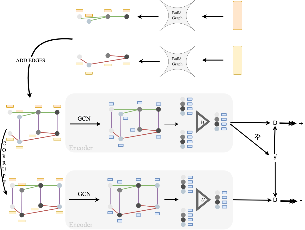
Figure 5.8: Build graph on concatenated features

5.3 Evaluation and results

In order to evaluate the quality of the proposed models, we have decided to proceed with two testing methods. Evaluation of the models on METABRIC dataset has one big problem which is that for one hyper-parameter setting 60 models need to be trained, in order to correctly evaluate the models performance. We thought that a synthetic dataset which needs to train only one model in order to asses the quality of a hyper-parameter setting would be more fitted, since it has only one label class would be helpful, and only one combination of modalities which can be integrated.

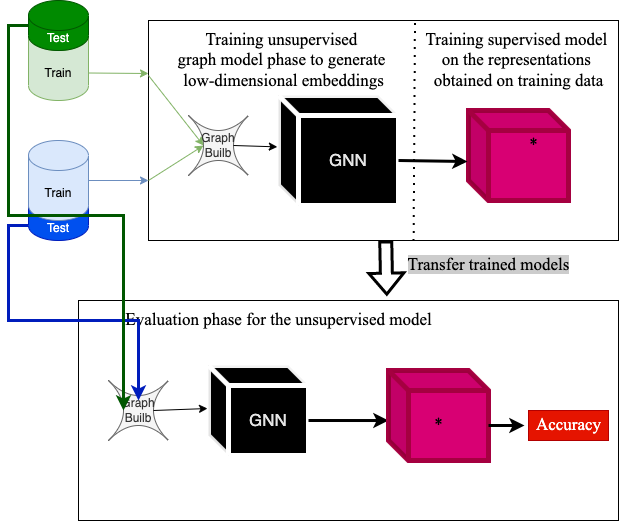
Figure 5.9: Evaluation pipeline for this project

The supervised models in use will be: Naive Bayes [M⁺06], Support Vector Machine [Nob06] and Random Forest [Qi12].

5.4 Evaluation on Synthetic-Data

In order to test these models on synthetic data, we have split each modality of the synthetic dataset in Training and Testing, with 75% of the samples for training and 25% of the samples for testing. While, a five-fold cross validation, would have been more suitable, the number of models we would have tested with different hyper-parameter settings would have been $\times 5$, because we need to re-train each model when the fold changes. The next subsections, will present the evaluation of CNC-DGI, CNC-VGAE, 2G-DGI and Hetero-DGI for various parameters.

CNC-DGI

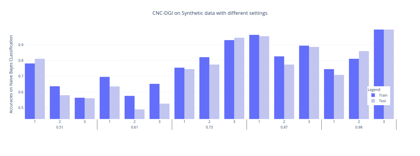
Figure 5.10: Accuracies of lower-latent representation obtained from CNC-DGI

For CNC-DGI the parameters chose are the depth of the Encoder, i.e. how many convolution layers there were going to be used $conv_{nr}=\{1,2,3\}$, in the context of five homophily levels $homophily_{levels}=\{0.51,0.61,0.73,0.87,0.98\}$.

CNC-VGAE

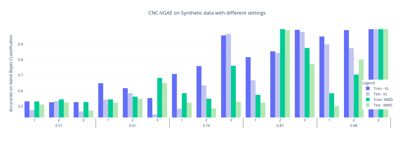
Figure 5.11: Accuracies of lower-latent representation obtained from CNC-VGAE

For CNC-VGAE the parameters chose are the depth of the Encoder $conv_{nr}=\{1,2,3\}$, and the reparametrisation loss function, which could be either MMD or KL diveregence loss, in the context of five homophily levels. From this diagram we can see that KL loss is more persistent as homophily levels increase, and as the number of layers increase. The best configuration for CNC-VAE can be with 3 GCN layers and using KL reparametrisation loss, even though [SBT⁺19] use MMD for reparametrisation loss. at the same time METABRIC homophily levels will be quite small maybe bellow 50% and from this diagram we can see that MDD gives better accuracies than KL on smaller homophily levels.

2G-DGI

For the 2G-DGI, the parameters chose where the number of convolution used from 1 to 3, and the concatenation layer shape (either dense layer or average), in the context of different homophily levels in $\{0.51,0.67,0.74,0.97\}$

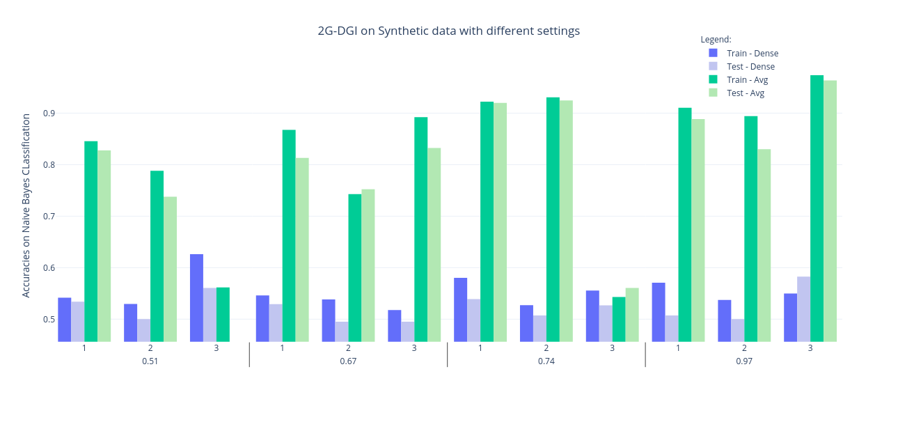
Figure 5.12: Accuracies of lower-latent representation obtained from 2G-DGI

One can see that, generally the results obtained with two GCN layers and with an average filter are better than the results obtained with a dense layer on other depths on the encoder, over various levels of homophily.

HeteroDGI

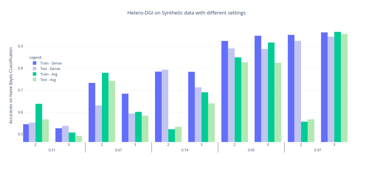
Figure 5.13: Accuracies of lower-latent representation obtained from Hetero-DGI

For the Hetero-DGI the evaluation setting is similar with 2G-DGI with the difference that encoders with one convolutional layers have been ignored. From the results one can learn that generally encoders with two convolutional layers work and with an dense layer give better results than all the other settings over various levels of homophily.

Conclusions

From these diagrams, one can learn that the homophily levels will greatly influence the quality of the lower-latent space representations produced by the proposed models. This means that when looking for best hyper-parameter setting for the METABRIC dataset, we should maximize the homophily levels of our graph by trying different values for $k$ (KNN) and $r$ Radius.

Since it can be noticed that for bigger homophily levels the accuracies also increase, we can conclude that the proposed models do separate the two classes of nodes for graph structures in which nodes with same class are favor an edge between them.

Another conclusion which can be drawn from the diagrams is that, the models do work. For example for homophily levels of 74%:

• CNC-VGAE will produce representations that will return 90% accuracy with a Naive Bayes classifier.

• CNC-DGI will produce representations that attain 90% accuracy with a Naive Bayes classifier.

• 2G-DGI will produce representations that attain an accuracy of 90% with a Naive Bayes classifier

• Hetero-DGI will produce representations that attain an accuracy of 80% with a Naive Bayes classifier

Another aspect that can be observed is that for small homophily, less layers of GCN give better result. This can happen because as the number of GCN layers increases, nodes will get information from further neighbours, which might be of different label, so not representative for the for the original node’s label.

5.5 Evaluation on METABRIC

This section, will introduce two evaluation procedures of the novel models on the METABRIC dataset. Since, the previous section has proved how increasing homophily levels also increase accuracies of the proposed models in the first evaluation experiment, we will carry experiments

5.5.1 Graph hyper-parameter selection

Since for pairs of modalities, and label class the construction of the graph is different the hyper-parameter search has been done on all pairs of modalities and all labels. What we have noticed is that the behavior of the results was constant through the modality change, but very different trough the label change class. Next, the results will be posted for all models on interaction of Clin+mRNA for all classes of labels.

The tests we will carry vary the value of $k\in\{2,4,16,64\}$ and $r\in\{0.005,0.05,0.5,1,5\}$. For all models the latent-lower space representation has 64 dimension. The dense layers have 128 dimensions. Each convolution has an PReLU (Parametric- ReLU) activation function. For each model in part the individual decisions we have took are:

• For CNC-VGAE in special the reparametrisation function will be MMD, even thought the synthetic dataset the results where questionable.

• For 2G-DGI the special integration layer will be a simple average of the two lower representations, because on the synthetic dataset

• For Hetero-DGI the special integration layer will be the dense layer

All the other tables can be find in the Appendix section.

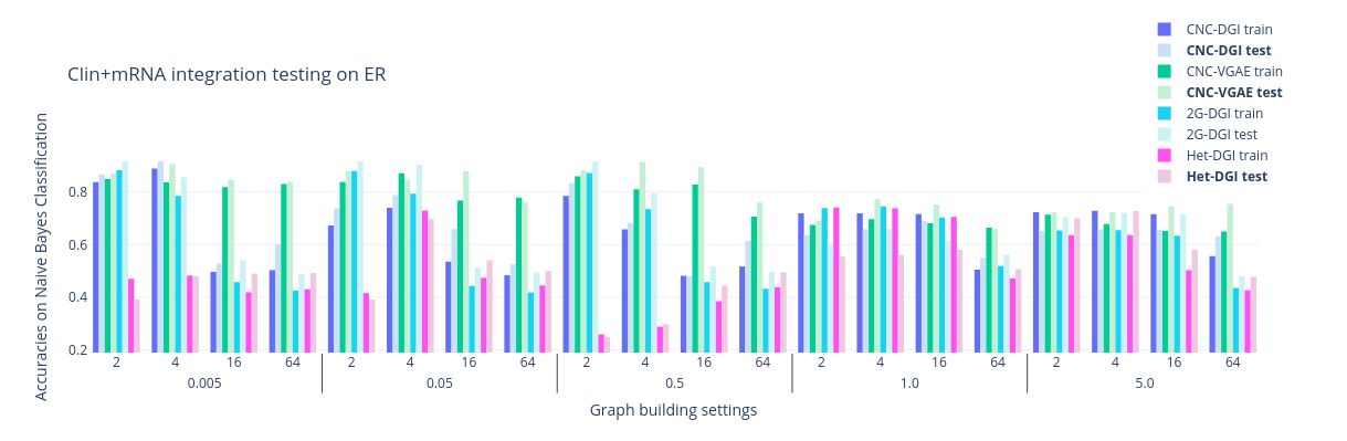
Figure 5.14: Accuracies of lower-latent representation obtained from CNC-VGAE

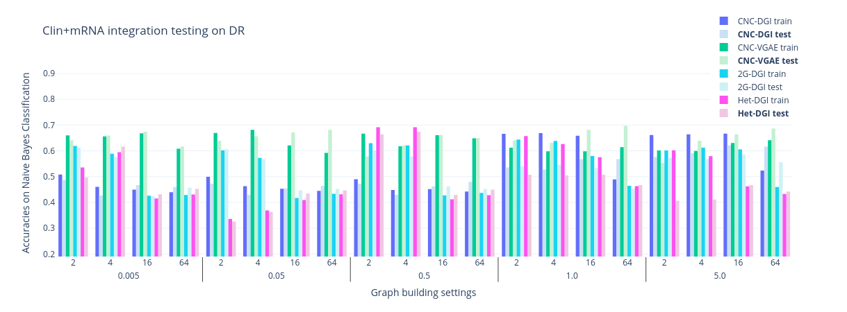
Figure 5.15: Accuracies of lower-latent representation obtained from CNC-VGAE

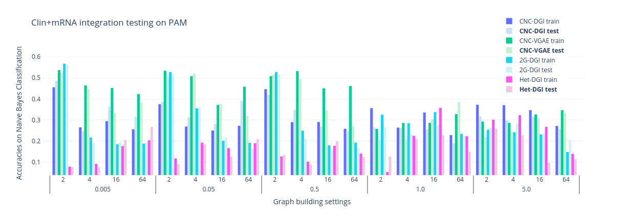
Figure 5.16: Accuracies of lower-latent representation obtained from CNC-VGAE

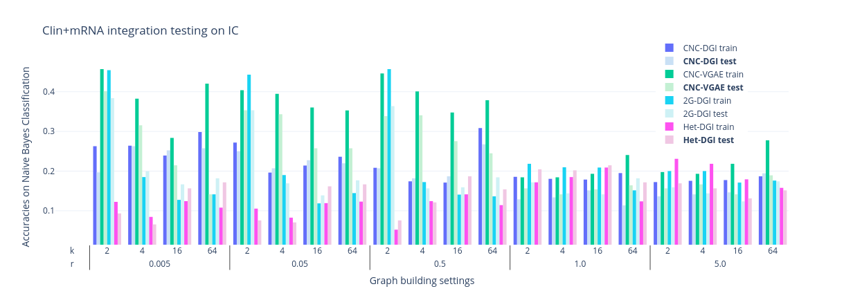
Figure 5.17: Accuracies of lower-latent representation obtained from CNC-VGAE

Best Model Assessment

		CNC-DGI			CNC-VGAE			2G-DGI			Hetero-DGI
		Clin+CNA	Clin+mRNA	CNA+mRNA	Clin+CNA	Clin+mRNA	CNA+mRNA	Clin+CNA	Clin+mRNA	CNA+mRNA	Clin+CNA	Clin+mRNA	CNA+mRNA
ER	NB	0.712	0.939	0.712	0.835	0.914	0.835	0.694	0.927	0.924	0.758	0.727	0.755
	SVM	0.793	0.919	0.881	0.841	0.914	0.851	0.773	0.929	0.939	0.763	0.770	0.768
	RF	0.841	0.934	0.891	0.833	0.909	0.833	0.806	0.924	0.937	0.795	0.823	0.806
DR	NB	0.636	0.621	0.676	0.68	0.696	0.694	0.689	0.614	0.679	0.692	0.674	0.694
	SVM	0.696	0.696	0.696	0.69	0.696	0.696	0.697	0.697	0.697	0.697	0.697	0.699
	RF	0.703	0.699	0.694	0.71	0.704	0.699	0.697	0.705	0.717	0.677	0.674	0.672
PAM	NB	0.312	0.487	0.381	0.398	0.398	0.449	0.553	0.563	0.298	0.412	0.268	0.194
	SVM	0.441	0.58	0.578	0.454	0.454	0.502	0.621	0.614	0.477	0.449	0.465	0.457
	RF	0.497	0.58	0.563	0.457	0.457	0.515	0.644	0.652	0.576	0.422	0.518	0.452
IC	NB	0.391	0.267	0.31	0.497	0.401	0.520	0.447	0.384	0.538	0.260	0.215	0.215
	SVM	0.458	0.387	0.454	0.482	0.414	0.532	0.467	0.482	0.593	0.391	0.278	0.338
	RF	0.5	0.447	0.515	0.474	0.383	0.527	0.465	0.500	0.621	0.422	0.407	0.381

Table 5.7: Best-in-class results on representations obtained with the models trained on various settings on classification task obtained with Naive Bayes Classifier, Support Vector Machine and Random Forest

From Table 5.7 we can clearly understand that 2G-DGI obtains best-in-class results, compared to the other models. A nice surprise is that on Clin+CNA on PAM class it actually beats the state of the art results, with $10\%$.

Even though, the architectures of the 2G-DGI and Hetero-DGI where similar in some sense, there is a clear difference between the best results obtained by both of them. This will be investigated in future work.

General unsatisfying results on IC label class, can be motivated by the low homophily levels of the produced graph on this label class (between 17%-19%).

Conclusions

From the above Figures (5.14, 5.15, 5.16, 5.17) we can learn the followings, individual comparisons per model:

• CNC-VGAE must give the best results out of all models in this testing settings, reason for which we will test the values it will return for the KL reparametrisation loss. For low values of r and k it returns best accuracies. For all classes of labels there seem to be a jump in average when transitioning from $r=0.5$ to $r=1$. Generally the difference between the testing accuracy and the training accuracy are small, sometimes testing accuracies are higher than the training ones.

• Hetero-DGI gives generally worse results than all the other models, this might be because the special integration layer is a dense layer, and not an average one. Also one can notice generally pick for high values of r, rather than changes in k, in fact it seems to decrease as k grows.

• CNC-DGI gives good results for the ER label, which has better homophily levels, where we can notice the average decreases as k increases. For DR label class, generally it gives good results when both $r$ and $k$ increase in value

• 2G-DGI returned competitive results with CNC-VGAE, which was a nice surprise. On ER the highest test accuracy is 87%, on DR is 69%, on PAM 57% (best out of all of them).

Specific on the label classes, we can learn the following:

• On ER, the models will return generally averages above 70%

• On DR for big values of both $r$ and $k$ the results will generally be above 60%

• On PAM most models return small accuracies (bellow 40%) with the exception on CNC-VGAE and 2G-DGI which will get to accuracies of 55% for values of $r$ smaller than $0.5$

• On IC most models will return small accuracies bellow 20%, but for small graphs 2G-DGI and CNC-VGAE can get to accuracies of 40%.

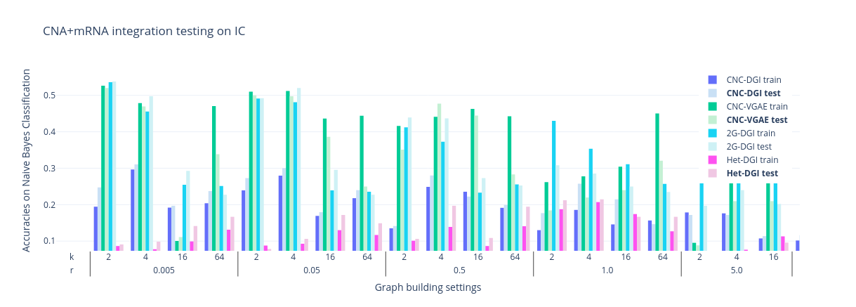
Figure 7.12: CNA+mRNA integration testing on IC

Generally, from the above conclusions we can learn, that there exist some correlation between the homophily levels described in Tables 5.1,5.2,5.3, 5.4, 5.5, 5.6 the number of edges in the graph, and the accuracies obtained. For Clin, homophily levels where around 16%, so this is a reason why IC on mRNA+Clin returns such small results. This exact fact can be proved by looking at Figure 7.12, which returns a best result of 53% accuracy on IC for CNA+mRNA integration. Intuitively, it’s almost like our learning process is downgraded by the high level of intra-class edges.

Chapter 6 Conclusion

6.1 Summary

This project presents the reader with a deep dive into a novel unsupervised learning pipeline leveraging Graph Neural Networks on a cancer classification task. We commenced by discussing and recreating the state-of-the-art models in “Variational Autoencoders for Cancer Data Integration: Design Principles and Computational Practice" [SBT⁺19], namely CNC-VAE and H-VAE. Our implementation of these architectures trained on the METABRIC dataset obtained results in line with the paper, and it provides a benchmark for the novel graph models proposed in our work.

• The integration of Clin+mRNA on the IC label class with CNC-VAE rendered $79\%$ accuracy

• The integration of CNA+mRNA and Clin+mRNA on the PAM label class resulted in $68\%$, and $73\%$ respective accuracies

• On all integration types of the ER label class, accuracies were above $85\%$

The following topic focused on graph construction algorithms on data sets which do not store relations between the data points representing our patients. These approaches include KNN, and generating links based on the Euclidean distance between nodes. We defined metrics quantifying the characteristics and overall quality of such graph data sets, such as homophily, and analysed the resulted graphs using these measurements. Generally, lower homophily levels resulted in very low accuracies in the lower-latent representation evaluation phase, while high levels of homophily achieved up to 99.8% accuracy. We can infer that the proposed models are sensitive to the graph structure of the input data.

During the design phase of the integrative models, we considered many factors such as the shape of the special integration layer being parametric or non-parametric, number of layers in the autoencoders as well as the number of neurons in each layer and many others. Hyper-parameter fine-tuning has been performed on each model for all pairs of modalities and for each class of labels, and the evaluation process has been in line with the that used in state-of-the-art works in order to ensure consistency.

To prove the functionality of the novel models, we introduced a synthetic dataset for which the results observed using generated lower-dimensional embeddings on classification tasks with Naive Bayes vary between 51% and 98% accuracy. Specifically, on each homophily class:

• For homophily level of 51%, 2G-DGI returned an accuracy of 82%, and CNC-DGI returned 80%.

• For homophily level of 61%, 2G-DGI returned an accuracy of 84%, and Hetero-DGI returned 79% accuracy.

• For higher homophily levels, we notice best-in-class results that are above 90%

Finally, as for the graph models applied on the METABRIC dataset, results vary much depending on the integrated modalities and on the label class, from 17% to 92%, in direct correlation with the homophily values of each label class. From Table 5.7 we can clearly understand that 2G-DGI obtains best-in-class results, compared to the other models. And we can also notice that on Clin+CNA integration on PAM with class it actually beats the state of the art results, with $10\%$.

6.2 Further work

During the development of the experiments in this projects and up to the report writing phase, we identified several opportunities to advance this line of research that could be tackled in the future. First, investing in the search of the most optimal hyper-parameters for the graph construction algorithms and Graph Neural Networks proposed in this paper can help improve the current results. Second, analysing and extending the number of integrated modalities with, for example, visual data, has the potential of discovering deeper insights into cancer sub-type cluster and cancer classification. Finally, we propose a novel model adapted from the Hierarchical Variational Autoencoder that introduces the use of Graph Convolutional Layers after the initial enconding phase. We conclude by presenting a mathematical problem regarding graph data that could be solved with probability theory and combinatorics.

Hyper-parameter settings

Given the multitude of architectural decisions required by the model training trials in this project, we intend to carry out more tests and search for the most optimal hyper-parameter settings that will further advance our architectures, such as the parameterised special integrative layer, the depth of the Encoder (i.e. number of GCN layers used), the size of the dense and latent space layers and so on.

Multi-modal expansion

The modalities integrated in this paper represent either continuous or categorical data - we intend to extend the integrative capabilities of the network to image data, and thus use more than two modalities. For the visual data, CNN layers can be added prior to the integration phase of the models to extract higher-level features from the input images.

H-VGAE

To advance the research avenue tackled in this project, we propose another model adapted from the Hierarchical Variational Autoencoder [SBT⁺19], which will be named Hierarchical Graph Variational Autoencoder (H-VGAE). The first processing units in this model are comprised of a series of autoencoders, that will generate a lower-latent representations independently for each input modality. A graph construction algorithm will be applied further to build relationships across the resulted embeddings, which will be fed among the lower-dimensional representations to two Graph Convolutional Layers: one aiming to find the mean and one to find the variance of the encoding distribution. Finally, the decoding phase consists of an inner product operation on the final representation, which will be compared to the originally built graph in the loss function.

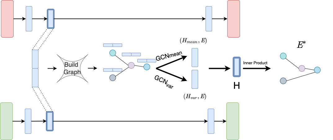
Figure 6.1: H-VGAE proposed architecture for integration

The reasons for which this model has the potential to render competitive results:

• The lower-dimensional embeddings generated by the first layer of autoencoders (one for each input modality) will lie on a continuous multi-Gaussian space. Hence, the radius algorithm for generating edges has a higher probability of returning dense graphs with better homophily levels than by using the method on its own.

• The closes model to this new architecture, CNC-VGAE, obtained among the best results across all tested models.

A Math Problem

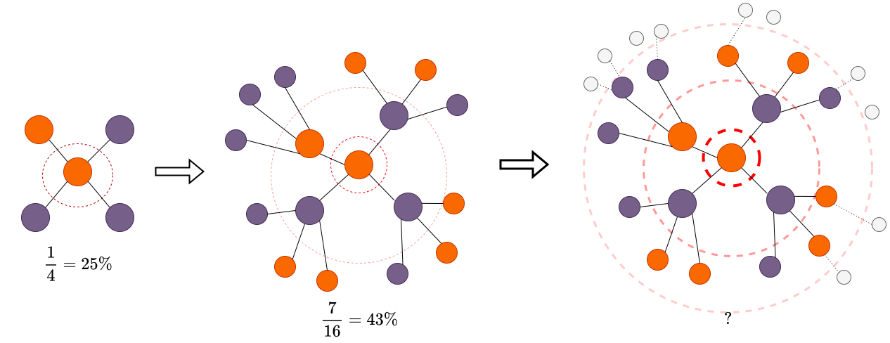
Figure 6.2: Growing neighbourhoods, and growing number of like neighbours

Take a graph with $25\%$ homophily level. Let O (orange) and P (purple) be two labels that the nodes can take, and let’s pick a node of label O. By taking the nodes immediate neighbourhood we expect that 1 out of 4 neighbours to be of label O, conversely for each P (purple) node we expect 3 orange neighbours and 1 purple neighbour. By taking a bigger neighbour, that includes immediate neighbours and their neighbours, we expect that 4 out of 10 to be of label O. This can be clearly understood from Figure 6.2. Our open ended question is if we continue increasing the neighborhoods can we reach a maximum for same label neighbours, will the number converge? Does this happen for classes that have more than two labels? What about different homophily levels? Can we generalize a formula?

This question can be relevant in this context because the number of growing nested neighbourhoods, can be the number of convolution layers that we apply, to a dataset with a certain homophily level. Attempting to answer this question might raise ideas on how learning on graphs with small homophily levels should be attempted.

Chapter 7 Appendix

7.1 Supplementary results

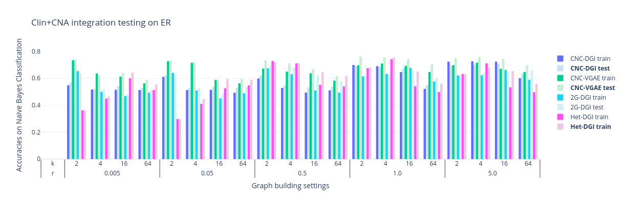
Figure 7.1: Clin+CNA integration testing on ER

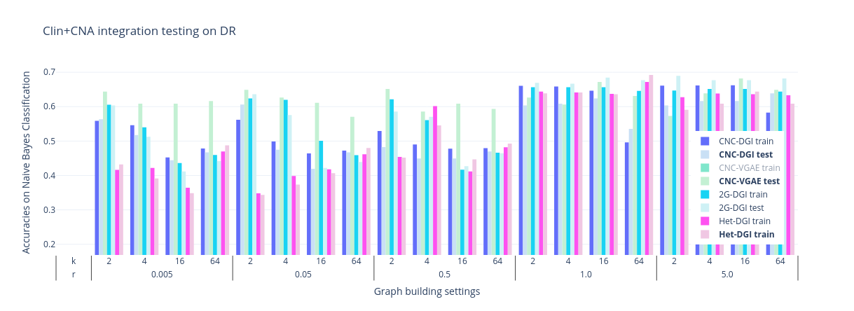
Figure 7.2: Clin+CNA integration testing on DR

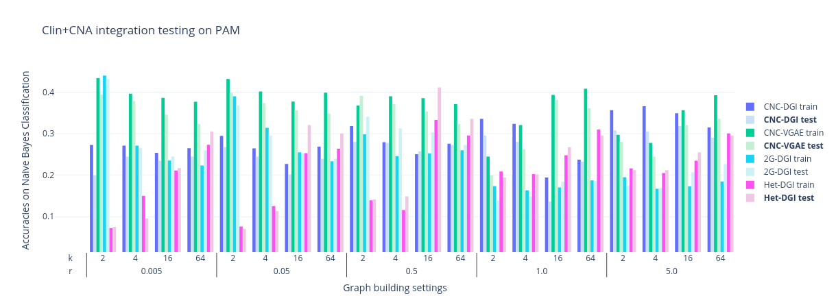
Figure 7.3: Clin+CNA integration testing on PAM

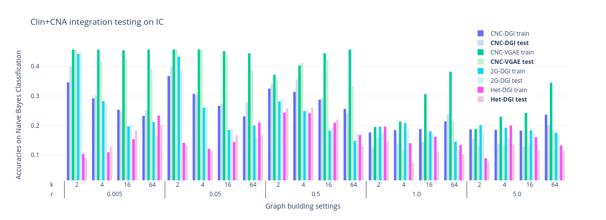
Figure 7.4: Clin+CNA integration testing on IC

Figure 7.5: Clin+mRNA integration testing on ER

Figure 7.6: Clin+mRNA integration testing on DR

Figure 7.7: Clin+mRNA integration testing on PAM

Figure 7.8: Clin+mRNA integration testing on IC

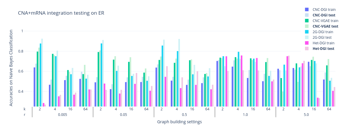
Figure 7.9: CNA+mRNA integration testing on ER

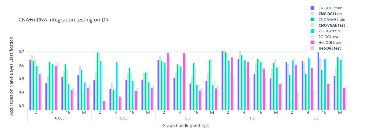
Figure 7.10: CNA+mRNA integration testing on DR

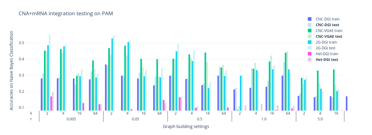
Figure 7.11: CNA+mRNA integration testing on PAM

References

- [AAB+16] Martín Abadi, Ashish Agarwal, Paul Barham, Eugene Brevdo, Zhifeng Chen, Craig Citro, Greg S Corrado, Andy Davis, Jeffrey Dean, Matthieu Devin, et al. Tensorflow: Large-scale machine learning on heterogeneous distributed systems. arXiv preprint arXiv:1603.04467, 2016.
- [AEHPK+19] Sami Abu-El-Haija, Bryan Perozzi, Amol Kapoor, Nazanin Alipourfard, Kristina Lerman, Hrayr Harutyunyan, Greg Ver Steeg, and Aram Galstyan. MixHop: Higher-order graph convolutional architectures via sparsified neighborhood mixing. In Kamalika Chaudhuri and Ruslan Salakhutdinov, editors, Proceedings of the 36th International Conference on Machine Learning, volume 97 of Proceedings of Machine Learning Research, pages 21–29. PMLR, 09–15 Jun 2019.
- [BC20] Nupur Biswas and Saikat Chakrabarti. Artificial intelligence (ai)-based systems biology approaches in multi-omics data analysis of cancer. Frontiers in Oncology, page 2224, 2020.
- [BG17] Aleksandar Bojchevski and Stephan Günnemann. Deep gaussian embedding of graphs: Unsupervised inductive learning via ranking. arXiv preprint arXiv:1707.03815, 2017.
- [BZSL13] Joan Bruna, Wojciech Zaremba, Arthur Szlam, and Yann LeCun. Spectral networks and locally connected networks on graphs. arXiv preprint arXiv:1312.6203, 2013.
- [C+18] Tabula Muris Consortium et al. Single-cell transcriptomics of 20 mouse organs creates a tabula muris. Nature, 562(7727):367–372, 2018.
- [CJP+18] Alfredo Massimiliano Cuzzocrea, Allan James, Norman W Paton, Srivastava Divesh, Agrawal Rakesh, Andrei Z Broder, Mohammed J Zaki, K Selçuk Candan, Labrinidis Alexandros, Schuster Assaf, et al. Proceedings of the 27th ACM International Conference on Information and Knowledge Management, CIKM 2018. ACM, 2018.
- [CNL11] Adam Coates, Andrew Ng, and Honglak Lee. An analysis of single-layer networks in unsupervised feature learning. In Proceedings of the fourteenth international conference on artificial intelligence and statistics, pages 215–223. JMLR Workshop and Conference Proceedings, 2011.
- [CPL+19] Kumardeep Chaudhary, Olivier B Poirion, Liangqun Lu, Sijia Huang, Travers Ching, and Lana X Garmire. Multimodal meta-analysis of 1,494 hepatocellular carcinoma samples reveals significant impact of consensus driver genes on phenotypes. Clinical Cancer Research, 25(2):463–472, 2019.
- [CPLG18] Kumardeep Chaudhary, Olivier B Poirion, Liangqun Lu, and Lana X Garmire. Deep learning–based multi-omics integration robustly predicts survival in liver cancer. Clinical Cancer Research, 24(6):1248–1259, 2018.
- [CPLM21] Eli Chien, Jianhao Peng, Pan Li, and Olgica Milenkovic. Adaptive universal generalized pagerank graph neural network. In International Conference on Learning Representations, 2021.
- [CSC+12] Christina Curtis, Sohrab P Shah, Suet-Feung Chin, Gulisa Turashvili, Oscar M Rueda, Mark J Dunning, Doug Speed, Andy G Lynch, Shamith Samarajiwa, Yinyin Yuan, et al. The genomic and transcriptomic architecture of 2,000 breast tumours reveals novel subgroups. Nature, 486(7403):346–352, 2012.
- [CSZ+17] Hao Chai, Xingjie Shi, Qingzhao Zhang, Qing Zhao, Yuan Huang, and Shuangge Ma. Analysis of cancer gene expression data with an assisted robust marker identification approach. Genetic epidemiology, 41(8):779–789, 2017.
- [Cyb89] George Cybenko. Approximation by superpositions of a sigmoidal function. Mathematics of control, signals and systems, 2(4):303–314, 1989.
- [DBV16] Michaël Defferrard, Xavier Bresson, and Pierre Vandergheynst. Convolutional neural networks on graphs with fast localized spectral filtering. Advances in neural information processing systems, 29, 2016.
- [DSLC+20] Carmen Lidia Diaz Soria, Jayhun Lee, Tracy Chong, Avril Coghlan, Alan Tracey, Matthew D Young, Tallulah Andrews, Christopher Hall, Bee Ling Ng, Kate Rawlinson, et al. Single-cell atlas of the first intra-mammalian developmental stage of the human parasite schistosoma mansoni. Nature communications, 11(1):1–16, 2020.
- [EGK+17] Joseph R Ecker, Daniel H Geschwind, Arnold R Kriegstein, John Ngai, Pavel Osten, Damon Polioudakis, Aviv Regev, Nenad Sestan, Ian R Wickersham, and Hongkui Zeng. The brain initiative cell census consortium: lessons learned toward generating a comprehensive brain cell atlas. Neuron, 96(3):542–557, 2017.
- [HFLM+18] R Devon Hjelm, Alex Fedorov, Samuel Lavoie-Marchildon, Karan Grewal, Phil Bachman, Adam Trischler, and Yoshua Bengio. Learning deep representations by mutual information estimation and maximization. arXiv preprint arXiv:1808.06670, 2018.
- [HYL17] Will Hamilton, Zhitao Ying, and Jure Leskovec. Inductive representation learning on large graphs. Advances in neural information processing systems, 30, 2017.
- [HZYZ21] Zongzhen He, Junying Zhang, Xiguo Yuan, and Yuanyuan Zhang. Integrating somatic mutations for breast cancer survival prediction using machine learning methods. Frontiers in genetics, page 1853, 2021.
- [KW13] Diederik P Kingma and Max Welling. Auto-encoding variational bayes. arXiv preprint arXiv:1312.6114, 2013.
- [KW16a] Thomas N Kipf and Max Welling. Semi-supervised classification with graph convolutional networks. arXiv preprint arXiv:1609.02907, 2016.
- [KW16b] Thomas N Kipf and Max Welling. Variational graph auto-encoders. arXiv preprint arXiv:1611.07308, 2016.
- [LHL+21] Derek Lim, Felix Hohne, Xiuyu Li, Sijia Linda Huang, Vaishnavi Gupta, Omkar Bhalerao, and Ser Nam Lim. Large scale learning on non-homophilous graphs: New benchmarks and strong simple methods. Advances in Neural Information Processing Systems, 34, 2021.
- [LJDW+22] Hongjie Li, Jasper Janssens, Maxime De Waegeneer, Sai Saroja Kolluru, Kristofer Davie, Vincent Gardeux, Wouter Saelens, Fabrice PA David, Maria Brbić, Katina Spanier, et al. Fly cell atlas: A single-nucleus transcriptomic atlas of the adult fruit fly. Science, 375(6584):eabk2432, 2022.
- [LZPX20] Bohyun Lee, Shuo Zhang, Aleksandar Poleksic, and Lei Xie. Heterogeneous multi-layered network model for omics data integration and analysis. Frontiers in genetics, page 1381, 2020.
- [M+06] Kevin P Murphy et al. Naive bayes classifiers. University of British Columbia, 18(60):1–8, 2006.
- [MTMG03] Stefano Monti, Pablo Tamayo, Jill Mesirov, and Todd Golub. Consensus clustering: a resampling-based method for class discovery and visualization of gene expression microarray data. Machine learning, 52(1):91–118, 2003.
- [MZ18] Tianle Ma and Aidong Zhang. Affinity network fusion and semi-supervised learning for cancer patient clustering. Methods, 145:16–24, 2018.
- [Nob06] William S Noble. What is a support vector machine? Nature biotechnology, 24(12):1565–1567, 2006.
- [PGM+19] Adam Paszke, Sam Gross, Francisco Massa, Adam Lerer, James Bradbury, Gregory Chanan, Trevor Killeen, Zeming Lin, Natalia Gimelshein, Luca Antiga, et al. Pytorch: An imperative style, high-performance deep learning library. Advances in neural information processing systems, 32, 2019.
- [PPK+] A Prat, JS Parker, O Karginova, C Fan, C Livasy, and JI Herschkowitz. and perou, cm (2010). phenotypic and molecular characterization of the claudin-low intrinsic subtype of breast cancer. Breast Cancer Research, 12:R68.
- [PSBB+21] Milan Picard, Marie-Pier Scott-Boyer, Antoine Bodein, Olivier Périn, and Arnaud Droit. Integration strategies of multi-omics data for machine learning analysis. Computational and Structural Biotechnology Journal, 19:3735–3746, 2021.
- [PWC+20] Hongbin Pei, Bingzhe Wei, Kevin Chen-Chuan Chang, Yu Lei, and Bo Yang. Geom-gcn: Geometric graph convolutional networks. arXiv preprint arXiv:2002.05287, 2020.
- [Qi12] Yanjun Qi. Random forest for bioinformatics. In Ensemble machine learning, pages 307–323. Springer, 2012.
- [RTL+17] Aviv Regev, Sarah A Teichmann, Eric S Lander, Ido Amit, Christophe Benoist, Ewan Birney, Bernd Bodenmiller, Peter Campbell, Piero Carninci, Menna Clatworthy, et al. Science forum: the human cell atlas. elife, 6:e27041, 2017.
- [SBT+19] Nikola Simidjievski, Cristian Bodnar, Ifrah Tariq, Paul Scherer, Helena Andres Terre, Zohreh Shams, Mateja Jamnik, and Pietro Liò. Variational autoencoders for cancer data integration: design principles and computational practice. Frontiers in genetics, 10:1205, 2019.
- [SNB+08] Prithviraj Sen, Galileo Namata, Mustafa Bilgic, Lise Getoor, Brian Galligher, and Tina Eliassi-Rad. Collective classification in network data. AI magazine, 29(3):93–93, 2008.
- [SWL18] Dongdong Sun, Minghui Wang, and Ao Li. A multimodal deep neural network for human breast cancer prognosis prediction by integrating multi-dimensional data. IEEE/ACM transactions on computational biology and bioinformatics, 16(3):841–850, 2018.
- [VCC+17] Petar Veličković, Guillem Cucurull, Arantxa Casanova, Adriana Romero, Pietro Lio, and Yoshua Bengio. Graph attention networks. arXiv preprint arXiv:1710.10903, 2017.
- [VFH+19] Petar Velickovic, William Fedus, William L Hamilton, Pietro Liò, Yoshua Bengio, and R Devon Hjelm. Deep graph infomax. ICLR (Poster), 2(3):4, 2019.
- [VLBM08] Pascal Vincent, Hugo Larochelle, Yoshua Bengio, and Pierre-Antoine Manzagol. Extracting and composing robust features with denoising autoencoders. In Proceedings of the 25th international conference on Machine learning, pages 1096–1103, 2008.
- [WBM+13] Wenting Wang, Veerabhadran Baladandayuthapani, Jeffrey S Morris, Bradley M Broom, Ganiraju Manyam, and Kim-Anh Do. ibag: integrative bayesian analysis of high-dimensional multiplatform genomics data. Bioinformatics, 29(2):149–159, 2013.
- [WJS+19] Xiao Wang, Houye Ji, Chuan Shi, Bai Wang, Yanfang Ye, Peng Cui, and Philip S Yu. Heterogeneous graph attention network. In The world wide web conference, pages 2022–2032, 2019.
- [WMD+14] Bo Wang, Aziz M Mezlini, Feyyaz Demir, Marc Fiume, Zhuowen Tu, Michael Brudno, Benjamin Haibe-Kains, and Anna Goldenberg. Similarity network fusion for aggregating data types on a genomic scale. Nature methods, 11(3):333–337, 2014.
- [WSH+20] Tongxin Wang, Wei Shao, Zhi Huang, Haixu Tang, Jie Zhang, Zhengming Ding, and Kun Huang. Moronet: multi-omics integration via graph convolutional networks for biomedical data classification. bioRxiv, 2020.
- [WZP+17] Bo Wang, Junjie Zhu, Emma Pierson, Daniele Ramazzotti, and Serafim Batzoglou. Visualization and analysis of single-cell rna-seq data by kernel-based similarity learning. Nature methods, 14(4):414–416, 2017.
- [XDK+19] Gangcai Xie, Chengliang Dong, Yinfei Kong, Jiang F Zhong, Mingyao Li, and Kai Wang. Group lasso regularized deep learning for cancer prognosis from multi-omics and clinical features. Genes, 10(3):240, 2019.
- [XWC+19] Jing Xu, Peng Wu, Yuehui Chen, Qingfang Meng, Hussain Dawood, and Hassan Dawood. A hierarchical integration deep flexible neural forest framework for cancer subtype classification by integrating multi-omics data. BMC bioinformatics, 20(1):1–11, 2019.
- [YK15] Aliaksandr A Yarmishyn and Igor V Kurochkin. Long noncoding rnas: a potential novel class of cancer biomarkers. Frontiers in genetics, 6:145, 2015.
- [You21] YourGenome. What is gene expression, 2021.
- [ZAL18] Marinka Zitnik, Monica Agrawal, and Jure Leskovec. Modeling polypharmacy side effects with graph convolutional networks. Bioinformatics, 34(13):i457–i466, 2018.
- [ZR20] Ron Zeira and Benjamin J Raphael. Copy number evolution with weighted aberrations in cancer. Bioinformatics, 36(Supplement_1):i344–i352, 2020.
- [ZYZ+20] Jiong Zhu, Yujun Yan, Lingxiao Zhao, Mark Heimann, Leman Akoglu, and Danai Koutra. Beyond homophily in graph neural networks: Current limitations and effective designs. Advances in Neural Information Processing Systems, 33:7793–7804, 2020.
- [ZZZM16] Ruoqing Zhu, Qing Zhao, Hongyu Zhao, and Shuangge Ma. Integrating multidimensional omics data for cancer outcome. Biostatistics, 17(4):605–618, 2016.