Time delay in the quadrupole field of a body at rest in 2PN approximation

Abstract

The time delay of a light signal in the quadrupole field of a body at rest is determined in the second post-Newtonian (2PN) approximation in harmonic coordinates. For grazing light rays at Sun, Jupiter, and Saturn the 2PN quadrupole effect in time delay amounts up to $0.004$, $0.14$, and $0.04$ pico-second, respectively. These values are compared with the time delay in the first post-Newtonian (1PN and 1.5PN) approximation, where it turns out that only the first eight mass-multipoles and the spin-dipole of these massive bodies are required for a given goal accuracy of $0.001$ pico-second in time-delay measurements in the solar system. In addition, the spin-hexapole of Jupiter is required on that scale of accuracy.

I Introduction

The time delay of a light signal in the gravitational field of a massive body was predicted by Shapiro in 1964 Shapiro1 and belongs to the four classical tests of general relativity: perihelion precession of Mercury, light deflection at the Sun, gravitational redshift of light, and light-travel time delay MTW . In its original formulation of the Shapiro effect one considers a light signal which propagates in the monopole field of one massive body with mass $M$ which is at rest with respect to the coordinate system.

Assume, the space-time is covered by harmonic coordinates, $\left(t,\mbox{\boldmath$x$}\right)$ MTW ; Poisson_Will ; Brumberg1991 ; Kopeikin_Efroimsky_Kaplan (cf. Eq. (5.177) in Poisson_Will ) and the origin of spatial axes is located at the center-of-mass of the massive body. The light signal is emitted by a light source at $\left(t_{0},\mbox{\boldmath$x$}_{0}\right)$ and then received by an observer at $\left(t_{1},\mbox{\boldmath$x$}_{1}\right)$. The Shapiro time delay is the difference between the light-travel-time, $\left(t_{1}-t_{0}\right)$, and the Euclidean distance between source and observer, $R=\left|\mbox{\boldmath$x$}_{1}-\mbox{\boldmath$x$}_{0}\right|$, divided by the speed of light,

$$\Delta\tau = \left(t_{1}-t_{0}\right)-\frac{R}{c}\;.$$ (1)

The Newtonian theory predicts no time delay. In General Relativity (GR), however, the light-travel-time $\left(t_{1}-t_{0}\right)$ differs from $R/c$, because the light signal propagates through the gravitational fields of the massive body, which decelerate the speed of the light signal. In first post-Newtonian (1PN) approximation for a massive body at rest the time delay is given by MTW ; Poisson_Will ; Brumberg1991

$$\Delta\tau^{M}_{\rm 1PN} = \frac{2GM}{c^{3}}\ln\frac{x_{1}+\mbox{\boldmath$k$}\cdot\mbox{\boldmath$x$}_{1}}{x_{0}+\mbox{\boldmath$k$}\cdot\mbox{\boldmath$x$}_{0}}\;,$$ (2)

where $\mbox{\boldmath$k$}=\left(\mbox{\boldmath$x$}_{1}-\mbox{\boldmath$x$}_{0}\right)/R$ is the unit-vector pointing from the source towards the observer; superscript label $M$ stands for monopole.

In the first time-delay measurements, performed in $1968$ Shapiro2 and $1971$ Shapiro3 , radar signals were emitted from Earth, which have passed nearby the limb of the Sun, then they were reflected by an inner planet, either Mercury or Venus, and finally the radar signals were received back on Earth. This round trip of the light signal is called two-way Shapiro effect and yields the double of Eq. (2) (cf. Eq. (10.102) in Poisson_Will ) which gives up to $248$ micro-seconds for the constellation Earth-Sun-Mercury, and amounts up to $251$ micro-seconds for the constellation Earth-Sun-Venus. In these experiments the time delay predicted by GR has been confirmed up to an error of a few percent, which corresponds to a precision in time measurements of a few micro-seconds. Ever since, time delay measurements have been performed with increasing accuracy. In $1977$ the Viking1 and Viking2 spacecrafts (Mars landers and orbiters) were used as radar reflectors, where an accuracy of about $0.5$ percent in time delay measurements was achieved Shapiro4 , which was later improved towards an accuracy of about $0.1$ percent Shapiro5 , which corresponds to a precision in time measurements of about $300$ nano-seconds. The most accurate time delay measurements in the solar system were achieved in $2003$ by using the Cassini spacecraft (orbiting Saturn) as reflector of the radar signals with an error of about $0.001$ percent Shapiro6 . The two-way Shapiro time delay for a grazing ray at the Sun for the configuration Earth-Sun-Saturn amounts up to $288$ micro-seconds, thus that error corresponds to an accuracy of a few nano-seconds in time delay measurements.

Future time-delay experiments will be performed by optical laser rather than radar signals, as suggested by several mission proposals of the European Space Agency (ESA) Astrod1 ; Lator1 ; Odyssey ; Sagas ; TIPO ; EGE . These missions are designed to significantly improve the test of relativistic gravity of the solar system. One aim of these experiments are time-delay measurements at the pico-second and sub-pico-second level of accuracy. In these mission proposals it has been suggested that a laser signal is emitted by the observer and then reflected by the spacecraft and afterwards received back by the observer. The decisive advantage of this two-way Shapiro effect is, that there is no need for clock-synchronization between observer and spacecraft Book_Clifford_Will . Thus, besides laser availability and reliability, significant improvements in measurements of the Shapiro effect are mainly dependent on advancements in the determination of the proper time at the observer’s position, either at ground stations or in space, which have made impressive progress during recent decades.

Today, accuracies on the sub-nano-second scale and even pico-second scale in time measurements are becoming standard in high-precision experiments in space. For instance, both Lunar Laser Ranging (LLR) as well as Satellite Laser Ranging (SLR) have reached the sub-nano-second and even the pico-second level of accuracy LLR1 ; LLR2 ; LLR3 ; SLR1 ; SLR2 ; Book_Soffel_Han which implies a standard deviation of the atomic clocks of about $\Delta t/t\sim 10^{-13}$. In these experiments a laser signal is sent from a ground station to the Moon or satellite, where it is reflected from retroreflectors, and then the laser signal is received back by the ground station; a review of LLR and future developments of SLR are given in SLR1 ; LLR4 . Meanwhile, there exists a global network of $45$ active ground stations which represent the International Laser Ranging Service. The measurement of the round-trip travel time allows one to determine the distance to the Moon or spacecraft, and such laser transfer measurements have reached the centimeter and even the millimeter level of accuracy, which corresponds to an accuracy of about $3$ pico-seconds in time measurements.

Furthermore, the two hydrogen maser atomic clocks onboard of each satellite of the European Galileo navigation system are mentioned, which have a standard deviation of $\Delta t/t\sim 10^{-14}$ which can be considered as minimal criterion for present-day technology of time measurements in space. The present-day most precise atomic clock onboard of a satellite is the Deep Space Atomic Clock (DSAC) DSAC1 launched in 2019 by National Aeronautics and Space Administration (NASA), which has a standard deviation of $\Delta t/t\sim 10^{-15}$. For a light signal in the solar system with a travel-time of about $10^{4}\,{\rm s}$ such a standard deviation of DSAC implies an accuracy of about $\Delta t\sim 10$ pico-second, which one may consider as minimal criterion for present-day technology of time measurements for the time-of-flight of such a light signal. In fact, by comparing DSAC to the U.S. Naval Observatory’s hydrogen maser master clock on the ground, the researchers found that the space clock deviates by about $26$ pico-seconds during one day DSAC_Nature . A follow-up project, DSAC-2, has recently been selected by NASA for demonstration on the upcoming space mission VERITAS (Venus Emissivity Radio Science Insar Topography and Spectroscopy) to Venus DSAC2 .

The atmosphere of the Earth has a significant impact on the speed and trajectory of light signals. In view of this fact, the advantage of space-based missions is that the atmosphere of Earth cannot disturb the time-of-flight measurements of light signals between spacecrafts. If ground-stations on Earth are involved in time-of-flight measurements, then the local meteorological data (i.e. altitude profile of temperature, pressure, humidity) need carefully to be determined with high accuracy during the period of time measurements. The modeling and description of atmospheric corrections of the ground-to-satellite time-transfer of light signals has made important advancements during recent years and has reached the pico-second level of accuracy ground_to_satellite . Thus, time-delay measurements with ground-stations remain an option also for future highly precise experiments on the pico-second and maybe on the sub-pico-second level.

As example of Earth-bound clocks are the Caesium atomic clocks NIST-F1 and NIST-F2 at the National Institute of Standard and Technology (NIST) are mentioned, where a standard deviation of $\Delta t/t\sim 10^{-16}$ has been achieved NIST . The highest accuracies for Earth-bound atomic clocks have been achieved with optical atomic clocks with a standard deviation of $\Delta t/t\sim 10^{-19}$ Atomic_Clock1 . If one considers a light signal emitted from Earth towards a spacecraft located in the solar system, for instance, nearby Uranus, and back, then the light-travel-time would be about $t\sim 10^{4}\,{\rm s}$. Hence, the standard deviation of such an atomic clock corresponds to a precision of about $\Delta t\sim 0.001$ pico-second, which one may consider as maximal criterion for present-day accuracy of time measurements for the time-of-flight of such a light signal, being aware that in near future the precision of optical atomic clocks will further be improved.

Accordingly, in consideration of these facts and being aware of further rapid progress in the precisions of time measurements in foreseen future Optical_Clocks1 , it seems necessary to develop the theoretical model of Shapiro time delay up to an accuracy of about $\Delta t=0.001$ pico-second. Also regarding the fact that a theoretical model should be at least one order of magnitude more precise than actual real measurements, this magnitude should be assumed as most upper accuracy threshold in theoretical considerations for prospective astrometry missions.

In view of these considerations it becomes apparent that the classical monopole formula (2) of time delay is by far not sufficient to meet near-future accuracies in time measurements and it is clear that the shape and inner structure of the bodies as well as their rotational motions become relevant on such scale of accuracy Zschocke_1PN ; Zschocke_15PN . The expansion of the metric tensor in terms of mass-multipoles, $\hat{M}_{L}$, and spin-multipoles, $\hat{S}_{L}$, of the massive solar system bodies allows one to account for these effects. The multipole expansion of the metric tensor implicates a corresponding multipole expansion of the Shapiro time-delay in terms of mass-multipoles and spin-multipoles. In particular, it is necessary to include some post-Newtonian terms (1PN and 1.5PN) in the theory of light propagation,

$$\Delta\tau = \sum\limits_{l=0}^{\infty}\Delta\tau_{\rm 1PN}^{M_{L}}+\sum\limits_{l=1}^{\infty}\Delta\tau_{\rm 1.5PN}^{S_{L}}+{\cal O}\left(c^{-4}\right),$$ (3)

where the first term $\left(l=0\right)$ is just the 1PN mass-monopole term as given by (2). It is clear that some of these higher mass-multipoles $\hat{M}_{L}$ (describe shape and inner structure of the massive body) and perhaps some spin-multipoles $\hat{S}_{L}$ (describe rotational motions and inner currents of the massive body) are relevant on the sub-pico-second level of accuracy. The mathematical expressions for the 1PN mass-multipole and 1.5PN spin-multipole terms in the Shapiro time delay, $\Delta\tau_{\rm 1PN}^{M_{L}}$ and $\Delta\tau_{\rm 1.5PN}^{S_{L}}$, were derived a long time ago Kopeikin1997 . It is one aim of this investigation to quantify these terms and to clarify which of these 1PN and 1.5PN terms need to be taken into account for the assumed goal accuracy of about $0.001$ pico-second.

Besides these 1PN and 1.5PN terms in (3) it might well be that also some 2PN terms are relevant on the sub-pico-second level of accuracy in time-delay measurements. For a long time, the knowledge about 2PN effects in the Shapiro time delay was restricted to the case of spherically symmetric bodies, that means in 2PN approximation only the mass-monopole term $M$ has been taken into account. The next subsequent term in the multipole decomposition is the mass-quadrupole term $M_{ab}$. Clearly, these terms are the most dominant 2PN terms beyond the 2PN mass-monopole. Recently, the light trajectory in 2PN approximation in the field of one body at rest with mass-monopole and mass-quadrupole structure was determined Zschocke_Quadrupole_1 . The investigation in Zschocke_Quadrupole_1 allows us to determine these 2PN mass-quadrupole terms in the Shapiro time-delay, that means

$$\Delta\tau = \Delta\tau_{\rm 1PN}^{M}+\Delta\tau_{\rm 1PN}^{M_{ab}}$$ (4)

$$+\,\Delta\tau_{\rm 2PN}^{M\times M}+\Delta\tau_{\rm 2PN}^{M\times M_{ab}}+\Delta\tau_{\rm 2PN}^{M_{ab}\times M_{cd}}+{\cal O}\left(c^{-6}\right).$$

In this investigation we will examine the impact of the 2PN monopole-monopole term, $\Delta\tau_{\rm 2PN}^{M\times M}$, the monopole-quadrupole term, $\Delta\tau_{\rm 2PN}^{M\times M_{ab}}$, and the quadrupole-quadrupole term, $\Delta\tau_{\rm 2PN}^{M_{ab}\times M_{cd}}$, and will compare them with the 1PN and 1.5PN terms in (3). Of course, the 1PN terms in (3) beyond the mass-quadrupole as well as the 1.5PN terms in (3) can finally be added to (4) in an appropriate manner.

The manuscript is organized as follows: In Section II the exact geodesic equation and the exact metric tensor for a body at rest is discussed. The 1PN and 1.5PN effect on the Shapiro time delay is determined in Section III. The initial value problem of the 2PN light propagation in the quadrupole field of one body at rest is considered in the Sections IV. The Shapiro time delay in 2PN approximation is examined in Section V. Finally a summary and outlook are given in Section VI. The notations as well as details of the calculations are relegated to a set of several Appendixes.

II Geodesic equation and metric tensor

A unique interpretation of astrometric observations, like the time-delay of light signals, requires the determination of light trajectory, $\mbox{\boldmath$x$}\left(t\right)$, as function of coordinate time. In Minkowskian space-time, a light signal would travel along a straight trajectory, the so-called unperturbed light ray. If the flat space-time is covered by Cartesian coordinates, the components of the Minkowskian metric read $\eta_{\alpha\beta}=\left(-1,+1,+1,+1\right)$ and then the trajectory of a light signal is given by

$$\mbox{\boldmath$x$}_{\rm N} = \mbox{\boldmath$x$}_{0}+c\left(t-t_{0}\right)\mbox{\boldmath$\sigma$}\;,$$ (5)

where the subindex ${\rm N}$ stands for Newtonian. That means a light signal, emitted at the spatial position of the light source, $\mbox{\boldmath$x$}_{0}$, would propagate along a straight line in the direction of some unit-vector $\sigma$. For graphical illustration of the unperturbed light trajectory see Figure 1.

The trajectory of a light signal propagating in curved space-time is determined by the geodesic equation (6) and isotropic condition (7), which in terms of coordinate time read as follows Brumberg1991 ; Kopeikin_Efroimsky_Kaplan ; MTW (e.g. Eqs. (1.2.48) - (1.2.49) in Brumberg1991 or Eqs. (7.20) - (7.23) in Kopeikin_Efroimsky_Kaplan ):

$$\frac{\ddot{x}^{i}\left(t\right)}{c^{2}}+\Gamma^{i}_{\mu\nu}\frac{\dot{x}^{\mu}\left(t\right)}{c}\frac{\dot{x}^{\nu}\left(t\right)}{c}-\Gamma^{0}_{\mu\nu}\frac{\dot{x}^{\mu}\left(t\right)}{c}\frac{\dot{x}^{\nu}\left(t\right)}{c}\frac{\dot{x}^{i}\left(t\right)}{c}=0\;,$$

(6)

$$g_{\alpha\beta}\,\frac{\dot{x}^{\alpha}\left(t\right)}{c}\,\frac{\dot{x}^{\beta}\left(t\right)}{c}=0\;,$$ (7)

where $g_{\alpha\beta}$ are the covariant components of the metric tensor of space-time; for the signature $\left(-,+,+,+\right)$ has been chosen. The isotropic condition (7) states that light trajectories are null rays, a condition which must be satisfied at any point along the light trajectory. Furthermore, a dot denotes total derivative with respect to coordinate time, and $\Gamma^{\alpha}_{\mu\nu}$ are the Christoffel symbols, given by Kopeikin_Efroimsky_Kaplan ; Brumberg1991 ; MTW (e.g. Eq.(21.27) in MTW )

$$\Gamma^{\alpha}_{\mu\nu}=\frac{1}{2}\,g^{\alpha\beta}\left(\frac{\partial g_{\beta\mu}}{\partial x^{\nu}}+\frac{\partial g_{\beta\nu}}{\partial x^{\mu}}-\frac{\partial g_{\mu\nu}}{\partial x^{\beta}}\right).$$ (8)

The Christoffel symbols are functions of the metric tensor. For weak gravitational fields it is meaningful to separate the metric tensor into the flat metric and a metric perturbation,

$$g_{\alpha\beta}\left(t,\mbox{\boldmath$x$}\right) = \eta_{\alpha\beta}+h_{\alpha\beta}\left(t,\mbox{\boldmath$x$}\right).$$ (9)

The geodesic equation is a differential equation of second order of one variable, $t$, thus a unique solution of (6) necessitates two initial-boundary conditions: the spatial position of light source $\mbox{\boldmath$x$}_{0}$ and the unit-direction $\sigma$ of the light signal at past infinity Brumberg1991 ; Kopeikin1997 ; KopeikinSchaefer1999_Gwinn_Eubanks ; KlionerKopeikin1992 ; Zschocke_1PN ; Zschocke_15PN :

$$\sigma = \frac{\dot{\mbox{\boldmath$x$}}\left(t\right)}{c}\,\bigg{|}_{t=-\infty}\quad{\rm with}\quad\mbox{\boldmath$\sigma$}\cdot\mbox{\boldmath$\sigma$}=1\;,$$ (10)

$$\mbox{\boldmath$x$}_{0}\; = \;\mbox{\boldmath$x$}\left(t\right)\bigg{|}_{t=t_{0}}\;.$$ (11)

Then, by inserting the decomposition (9) into (6) and using the initial-boundary conditions (10) and (11), the solution of the second integration of geodesic equation (trajectory of light signal) (6) is given by

$$\mbox{\boldmath$x$}\left(t\right) = \mbox{\boldmath$x$}_{0}+c\left(t-t_{0}\right)\mbox{\boldmath$\sigma$}+\Delta\mbox{\boldmath$x$}\left(t,t_{0}\right),$$ (12)

where $\Delta\mbox{\boldmath$x$}$ is the correction to the trajectory of the unperturbed light ray (5). The formal solution of the initial value problem (12) implies the following limit,

$$\lim_{t\rightarrow t_{0}}\Delta\mbox{\boldmath$x$}\left(t,t_{0}\right) = 0\;,$$ (13)

in order to be consistent with the condition (11).

For solving the geodesic equation (6) one needs the metric tensor (9) of the specific problem under consideration. Usually, the metric tensor (9) is not known in its exact form and one has to apply for some approximation scheme. If the gravitational fields are weak and the speed of matter is slow compared to the speed of light, then one can utilize the post-Newtonian expansion (weak-field slow-motion expansion) of the metric tensor, which is an expansion of the metric tensor in inverse powers of the speed of light Thorne ; Blanchet_Damour1 ,

$$g_{\alpha\beta}\left(t,\mbox{\boldmath$x$}\right) = \eta_{\alpha\beta}+\sum\limits_{n=2}^{\infty}h^{\left({\rm n}\right)}_{\alpha\beta}\left(t,\mbox{\boldmath$x$},\ln c\right).$$ (14)

In general, the post-Newtonian expansion (14) is a non-analytic series, because at higher order $n\geq 8$ non-analytic terms involving powers of logarithms occur Thorne ; Blanchet_Damour1 , while by definition the $n$-th post-Newtonian perturbation, $h^{\left({\rm n}\right)}_{\alpha\beta}$, is the factor of $n$-th inverse power of $c$.

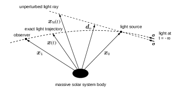
Figure 1: A geometrical representation of the propagation of a light signal through the gravitational field of a massive solar system body at rest. The light signal is emitted by the light source at $\mbox{\boldmath$x$}_{0}$ and propagates along the exact light trajectory $\mbox{\boldmath$x$}\left(t\right)$. The unit tangent vector along the light trajectory at past null infinity is $\sigma$. The unperturbed light ray $\mbox{\boldmath$x$}_{\rm N}\left(t\right)$ is given by Eq. (5) and propagates in the direction of $\sigma$ along a straight line through the position of the light source at $\mbox{\boldmath$x$}_{0}$. The impact vector $\mbox{\boldmath$d$}_{\sigma}$ of the unperturbed light ray is given by Eq. (57). The impact vector $\hat{\mbox{\boldmath$d$}_{\sigma}}$ is defined by Eq. (324) and is parallel to the impact vector $\mbox{\boldmath$d$}_{\sigma}$ but a tiny bit smaller and not shown in the diagram.

In reality, a solar system body can be of arbitrary shape, inner structure, rotational and oscillating motions and can have inner currents of matter. From the Multipolar Post-Minkowskian (MPM) formalism Thorne ; Blanchet_Damour1 ; Blanchet6 it follows that the post-Newtonian solution for the metric tensor for such a body can be given in terms of two kinds of symmetric and trace-free (STF) multipoles: mass-multipoles $\hat{M}_{L}$ (describing shape, inner structure and oscillations of the body) and spin-multipoles $\hat{S}_{L}$ (describing rotational motions and inner currents of the body)

$$g_{\alpha\beta}\left(t,\mbox{\boldmath$x$}\right) = \eta_{\alpha\beta}+\sum\limits_{n=2}^{\infty}h^{\left({\rm n}\right)}_{\alpha\beta}(\hat{M}_{L}\left(s\right),\hat{S}_{L}\left(s\right),\ln c)$$ (15)

where the origin of spatial axes of the coordinate system is located somewhere nearby the center of mass of the source of matter (body), and $s=t-x/c$ is the retarded time which describes the fact that the metric at field point $\left(t,\mbox{\boldmath$x$}\right)$ is determined by the multipoles at the earlier time $s$ because gravitational action propagates with the finite speed of light. In case of a stationary source of matter the multipoles and the metric perturbations are time-independent and then the post-Newtonian expansion of the metric tensor reads

$$g_{\alpha\beta}\left(\mbox{\boldmath$x$}\right) = \eta_{\alpha\beta}+\sum\limits_{n=2}^{\infty}h^{\left({\rm n}\right)}_{\alpha\beta}(\hat{M}_{L},\hat{S}_{L},\ln c).$$ (16)

These multipoles $\hat{M}_{L}$ and $\hat{S}_{L}$ in (15) and (16) are integrals over the stress-energy tensor of the source of matter. They are considered in Appendix B.

III Shapiro effect in 1.5PN approximation

In 1.5PN approximation the expansion (16) reads

$$g_{\alpha\beta} = \eta_{\alpha\beta}+h_{\alpha\beta}^{\left(2\right)}(\hat{M}_{L})+h_{\alpha\beta}^{\left(3\right)}(\hat{S}_{L})$$ (17)

up to terms of the order ${\cal O}(c^{-4})$, and where the non-vanishing metric perturbations $h_{\alpha\beta}^{\left(2\right)}$ and $h_{\alpha\beta}^{\left(3\right)}$ are given by Thorne ; Blanchet_Damour1 ; Multipole_Damour_2 ; Kopeikin1997 ; Zschocke_2PM_Metric

$$h_{00}^{\left(2\right)} = +\frac{2}{c^{2}}\sum\limits_{l=0}^{\infty}\frac{\left(-1\right)^{l}}{l!}\,\hat{M}_{L}\,\hat{\partial}_{L}\frac{1}{r}\;,$$ (18)

$$h_{0i}^{\left(3\right)} = +\frac{4}{c^{3}}\sum\limits_{l=1}^{\infty}\frac{\left(-1\right)^{l}\,l}{\left(l+1\right)!}\,\epsilon_{iab}\,\hat{S}_{bL-1}\,\hat{\partial}_{aL-1}\frac{1}{r}\;,$$ (19)

$$h_{ij}^{\left(2\right)} = +\frac{2}{c^{2}}\,\delta_{ij}\sum\limits_{l=0}^{\infty}\frac{\left(-1\right)^{l}}{l!}\,\hat{M}_{L}\,\hat{\partial}_{L}\frac{1}{r}\;,$$ (20)

where $r=\left|\mbox{\boldmath$x$}\right|$ and

$$\hat{\partial}_{L}={\rm STF}_{i_{1}\dots i_{l}}\,\partial_{i_{1}}\dots\partial_{i_{l}}\;.$$ (21)

The mass-multipoles and spin-multipoles in (18) - (20) in case of stationary source of matter are given by

$$\hat{M}_{L} = \int d^{3}x\;\hat{x}_{L}\;\Sigma\,,$$ (22)

$$\hat{S}_{L} = \int d^{3}x\;\epsilon_{jk<i_{l}}\,\hat{x}_{L-1>}\;x^{j}\;\Sigma^{k}\,,$$ (23)

where the notation $\Sigma=\left(T^{00}+T^{kk}\right)/c^{2}$ and $\Sigma^{k}=T^{0k}/c$ has been adopted, with $T^{\alpha\beta}$ being the stress-energy tensor of the body, and where the integrals run over the three-dimensional volume of the body. The geodesic equation in 1.5PN approximation can be deduced from the exact geodesic equation (6) and is given by Eq. (2.2.49) in Brumberg1991 (up to a global sign convention). Inserting the metric perturbations (18) - (20) into the geodesic equation in 1.5PN approximation yields

$$\frac{\ddot{\mbox{\boldmath$x$}}}{c^{2}} = \sum\limits_{l=0}^{\infty}\frac{\ddot{\mbox{\boldmath$x$}}_{\rm 1PN}^{M_{L}}}{c^{2}}+\sum\limits_{l=1}^{\infty}\frac{\ddot{\mbox{\boldmath$x$}}_{\rm 1.5PN}^{S_{L}}}{c^{2}}$$ (24)

up to terms of the order ${\cal O}(c^{-4})$, and where $\ddot{\mbox{\boldmath$x$}}_{\rm 1PN}^{M_{L}}$ and $\ddot{\mbox{\boldmath$x$}}_{\rm 1.5PN}^{S_{L}}$ are given by Eq. (13) in Kopeikin1997 . The solution of (24) reads formally as follows:

$$\mbox{\boldmath$x$}\left(t\right) = \mbox{\boldmath$x$}_{0}+c\left(t-t_{0}\right)\mbox{\boldmath$\sigma$}+\sum\limits_{l=0}^{\infty}\Delta\mbox{\boldmath$x$}^{M_{L}}_{\rm 1PN}+\sum\limits_{l=1}^{\infty}\Delta\mbox{\boldmath$x$}^{S_{L}}_{\rm 1.5PN}$$

up to terms of the order ${\cal O}(c^{-4})$, and where $\Delta\mbox{\boldmath$x$}_{\rm nPN}={\cal O}\left(c^{-2n}\right)$.

Table 1: Numerical parameter for mass $M$, radius $P$, actual zonal harmonic coefficients $J_{l}$, distance between observer and body $x_{1}$, of Sun, Jupiter and Saturn. The values for $GM/c^{2}$ and $P$ are taken from Ellipticity . The value for $J_{l}$ for the Sun are taken from J_n_Sun and references therein. The values $J_{l}$ with $n=2,4,6$ for Jupiter and Saturn are taken from Book_Zonal_Harmonics , while $J_{l}$ with $n=8,10$ for Jupiter and Saturn are taken from Zonal_Harmonics_Jupiter and Zonal_Harmonics_Saturn , respectively. The angular velocity $\Omega=2\pi/T$ (with rotational period $T$) are taken from NASA planetary fact sheets. The dimensionless moment of inertia $\kappa^{2}$ is defined by Eq. (152) and their values are taken from Ellipticity . For the distance between light-source and body we assume $x_{0}=10^{11}\,{\rm m}$ so that the light-source is within the near-zone of the Solar system, while $x_{1}$ is computed under the assumption that the observer (spacecraft) is located at Lagrange point $L_{2}$, i.e. $1.5\times 10^{9}\,{\rm m}$ from Earth.

Parameter	Sun	Jupiter	Saturn
$GM/c^{2}\,[{\rm m}]$	$1476.8$	$1.41$	$0.42$
$P\,[{\rm m}]$	$696\times 10^{6}$	$71.5\times 10^{6}$	$60.3\times 10^{6}$
$J_{2}$	$1.7\times 10^{-7}$	$14.696\times 10^{-3}$	$16.291\times 10^{-3}$
$J_{4}$	$9.8\times 10^{-7}$	$-0.587\times 10^{-3}$	$-0.936\times 10^{-3}$
$J_{6}$	$4\times 10^{-8}$	$0.034\times 10^{-3}$	$0.086\times 10^{-3}$
$J_{8}$	$-4\times 10^{-9}$	$-2.5\times 10^{-6}$	$-10.0\times 10^{-6}$
$J_{10}$	$-2\times 10^{-10}$	$0.21\times 10^{-6}$	$2.0\times 10^{-6}$
$\Omega\,[{\rm sec}^{-1}]$	$2.865\times 10^{-6}$	$1.758\times 10^{-4}$	$1.638\times 10^{-4}$
$\kappa^{2}$	$0.059$	$0.254$	$0.210$
$x_{1}\,[{\rm m}]$	$0.150\times 10^{12}$	$0.59\times 10^{12}$	$1.20\times 10^{12}$

In Kopeikin1997 advanced integration methods have been introduced which allow to integrate (24) exactly and which lead to the exact expression of (LABEL:Second_Interation_1PN), given by Eqs. (33), (36) and (38) in Kopeikin1997 . In that approach two new parameters were introduced,

$$c\tau = \mbox{\boldmath$\sigma$}\cdot\mbox{\boldmath$x$}_{\rm N}\;,$$ (26)

$$\xi^{i} = P^{i}_{j}\,x_{\rm N}^{j}\;,$$ (27)

where $P^{ij}=\delta^{ij}-\sigma^{i}\sigma^{j}$ is a projection operator onto the plane perpendicular to vector $\sigma$; note that $P^{ij}=P_{ij}=P^{i}_{j}$. Obviously, the unperturbed light ray (5) expressed in terms of these new variables takes the form

$$\mbox{\boldmath$x$}_{\rm N} = \mbox{\boldmath$\xi$}+c\tau\,\mbox{\boldmath$\sigma$}\;.$$ (28)

The three-vector $\xi$ is laying in the two-dimensional plane perpendicular to $\sigma$, hence only two components are independent, which implies $\partial\xi^{i}/\partial\xi^{j}=P^{i}_{j}$. But in practical calculations it is convenient to treat the spatial components of this vector as formally independent, which implies $\partial\xi^{i}/\partial\xi^{j}=\delta^{i}_{j}$. Therefore, a subsequent projection onto this two-dimensional plane by means of $P^{ij}$ is necessary (cf. text above Eq. (31) in KopeikinSchaefer1999_Gwinn_Eubanks as well as Eqs. (11.2.12) and (11.2.13) in Book_Soffel_Han ). Then, for a spatial derivative expressed in terms of these new variables, one obtains

$$\frac{\partial}{\partial x^{i}} = P_{i}^{j}\,\frac{\partial}{\partial\xi^{j}}+\sigma_{i}\,\frac{\partial}{\partial c\tau}\;.$$ (29)

In case of time-independent functions, relation (33) in KopeikinSchaefer1999_Gwinn_Eubanks coincides with relation (29). Then, using (29) and the binomial theorem, one finds the differential operator in (21) expressed in terms of these new variables,

$$\hat{\partial}_{L} = {\rm STF}_{i_{1}\dots i_{l}}\;\sum\limits_{p=0}^{l}\frac{l!}{\left(l-p\right)!\;p!}\;\sigma_{i_{1}}\,...\,\sigma_{i_{p}}$$ (30)

$$\times\,P_{i_{p+1}}^{j_{p+1}}\;...\;P_{i_{l}}^{j_{l}}\;\frac{\partial}{\partial\xi^{j_{p+1}}}\;...\;\frac{\partial}{\partial\xi^{j_{l}}}\;\left(\frac{\partial}{\partial c\tau}\right)^{p}\,.$$

Here we prefer to use the operator as given by Eq. (30) where $\partial\xi^{i}/\partial\xi^{j}=\delta^{i}_{j}$, while if one applies the operator as given by Eq. (24) in Kopeikin1997 then $\partial\xi^{i}/\partial\xi^{j}=P^{i}_{j}$. The results of either these operations are identical. Then, using the basic integral (25) in Kopeikin1997 one finds for the second integration the formulas given by Eq. (27) in Kopeikin1997 , which lead to the solution for the second integration of geodesic equation (24).

The approach introduced in Kopeikin1997 for bodies at rest and time-independent multipoles has further been developed for the case of light propagation in the gravitational field of a time-dependent source of matter at rest KopeikinSchaefer1999_Gwinn_Eubanks ; KopeikinKorobkovPolnarev2006 ; KopeikinKorobkov2005 , as well as in the gravitational field of $N$ slowly moving bodies with time-dependent multipoles in our investigations in Zschocke_1PN ; Zschocke_15PN .

According to the solution for the light trajectory as given by Eq. (31) with (33), (36), (38) in Kopeikin1997 , the time-of-flight in the gravitational field of a body with full mass-multipole and spin-multipole structure is given by the following formula (cf. Eq. (40) in Kopeikin1997 ),

$$c\left(t_{1}-t_{0}\right) = R+\sum\limits_{l=0}^{\infty}\Delta c\tau_{\rm 1PN}^{M_{L}}+\sum\limits_{l=1}^{\infty}\Delta c\tau_{\rm 1.5PN}^{S_{L}}$$ (31)

up to terms of the order ${\cal O}(c^{-4})$. The mass-multipole (gravitoelectric) term reads (cf. Eqs. (41) and (42) in Kopeikin1997 )

$$\Delta c\tau_{\rm 1PN}^{M_{L}} = +\frac{2G}{c^{2}}\frac{\left(-1\right)^{l}}{l!}\hat{M}_{L}$$

$$\times\left(\hat{\partial}_{L}\,\ln\left(r_{\rm N}+c\tau\right)\bigg{|}_{\tau=t_{1}}-\hat{\partial}_{L}\,\ln\left(r_{\rm N}+c\tau\right)\bigg{|}_{\tau=t_{0}}\right),$$

and the spin-multipole (gravitomagnetic) term reads (cf. Eq. (43) in Kopeikin1997 ; note an overall sign error in Eq. (43) in Kopeikin1997 ; see also footnote $3$ in Ciufolini as well as Ref. $\left[73\right]$ in Zschocke_15PN )

$$\Delta c\tau_{\rm 1.5PN}^{S_{L}} = +\frac{4G}{c^{3}}\frac{\left(-1\right)^{l}\,l}{\left(l+1\right)!}\,\sigma_{i}\,\epsilon^{iab}\,\hat{S}_{bL-1}$$

$$\times\left(\!\hat{\partial}_{aL-1}\ln\left(r_{\rm N}+c\tau\right)\bigg{|}_{\tau=t_{1}}-\hat{\partial}_{aL-1}\ln\left(r_{\rm N}+c\tau\right)\bigg{|}_{\tau=t_{0}}\right),$$

where $r_{\rm N}=\left|\mbox{\boldmath$x$}_{\rm N}\right|$ with $\mbox{\boldmath$x$}_{\rm N}$ in (28), that means $r_{\rm N}=\sqrt{\xi^{2}+c^{2}\tau^{2}}$. These equations were also given by Eqs. (11.2.34) and (11.2.35) in Book_Soffel_Han . In (LABEL:Shapiro_Mass_Multipole) and (LABEL:Shapiro_Spin_Multipole) the differentiations have to be performed. Afterwards one has to substitute the unperturbed light ray by the standard expression as given by Eq. (5) where the coordinate time is either $t_{1}$ or $t_{0}$ as indicated by the sub-labels. In particular, at the very end of the calculations one has to replace $c\tau$ by $\mbox{\boldmath$\sigma$}\cdot\mbox{\boldmath$x$}_{\rm N}$ and $\xi$ by $\mbox{\boldmath$d$}_{\sigma}$. For details about how to perform the differentiations the reader is referred to Kopeikin1997 ; Book_Soffel_Han . Because the mass-quadrupole is of specific relevance in our investigation, we consider the application of (LABEL:Shapiro_Mass_Multipole) for the mass-quadrupole explicitly in Appendix C.

The largest effect of Shapiro effect is expected from the Sun and the giant planets of the solar system. In order to determine the Shapiro time delay one needs the explicit form for mass-multipoles (22) and for spin-multipoles (23). For an estimation of the individual terms in (LABEL:Shapiro_Mass_Multipole) and (LABEL:Shapiro_Spin_Multipole), one may approximate the Sun and the giant planets by a rigid axisymmetric body with radial dependent mass distribution and in uniform rotational motion around the symmetry axis of the body, which is aligned with the $x^{3}$-axis of the coordinate system. Then, the higher mass-multipoles for such a body are given by Eqs. (126) in Appendix B, while the spin-dipole and higher spin-multipoles for such a body are given by Eq. (154) and Eq. (148) in Appendix B:

$$\hat{M}_{0} = M\;,$$ (34)

$$\hat{M}_{L} = -M\left(P\right)^{l}\,J_{l}\;\delta^{3}_{<{i_{1}}}\;\dots\;\delta^{3}_{{i_{l}}>}$$

$${\rm with}\quad l=2,4,6,\dots\;,$$

$$\hat{S}_{a} = \kappa^{2}\,M\,\Omega\,P^{2}\,\delta_{3a}\;,$$ (36)

$$\hat{S}_{L} = -M\,\Omega\left(P\right)^{l+1}\,J_{l-1}\,\frac{l+1}{l+4}\;\delta^{3}_{<{i_{1}}}\;\dots\;\delta^{3}_{{i_{l}}>}$$

$${\rm with}\quad l=3,5,7,\dots\;,$$

where $M$ is the Newtonian mass of the body, $P$ its equatorial radius, $J_{l}$ are the actual zonal harmonic coefficients of index $l$, $\kappa^{2}$ is the dimensionless moment of inertia, $\Omega$ is the angular velocity of the rotating body and $\delta^{3}_{<{i_{1}}}\;\dots\;\delta^{3}_{{i_{l}}>}={\rm STF}_{i_{1}\dots i_{l}}\;\delta_{3i_{1}}\dots\delta_{3i_{l}}$ denotes products of Kronecker symbols which are symmetric and traceless with respect to indices $i_{1}\dots i_{l}$. These multipoles (III) and (III) are in agreement with the multipoles for an rigid axisymmetric body in uniform rotational motion as given in the resolutions of the International Astronomical Union (IAU) IAU_Resolution1 ; that agreement is shown explicitly in Appendix B for the mass-quadrupole as well as for the spin-hexapole in case of a rigid axisymmetric body with uniform mass-density.

The calculations can considerably be simplified by inserting the mass-multipoles and spin-multipoles (III) and (III) into (LABEL:Shapiro_Mass_Multipole) and (LABEL:Shapiro_Spin_Multipole), respectively, and afterwards one starts with the evaluation of the Shapiro time delay. Then, one obtains the following upper limits of the individual terms of Shapiro time delay (cf. text below Eq. (43) in Kopeikin1997 ):

$$\left|\Delta\tau_{\rm 1PN}^{M}\right| \leq 2\,\frac{GM}{c^{3}}\,\ln\frac{4\,x_{0}\,x_{1}}{\left(d_{\sigma}\right)^{2}}\;,$$ (38)

$$\left|\Delta\tau_{\rm 1PN}^{M_{L}}\right| \leq A_{l}\,\frac{GM}{c^{3}}\,\left|J_{l}\right|\left(\frac{P}{d_{\sigma}}\right)^{l}$$

$${\rm with}\quad l=2,4,6,\dots\;,$$

$$\left|\Delta\tau_{\rm 1.5PN}^{S}\right| \leq 4\,\frac{GM}{c^{4}}\,\kappa^{2}\,P\,\Omega\;,$$ (40)

$$\left|\Delta\tau_{\rm 1.5PN}^{S_{L}}\right| \leq B_{l}\,\frac{GM}{c^{4}}\,P\,\Omega\,\left|J_{l-1}\right|\left(\frac{P}{d_{\sigma}}\right)^{l}$$

$${\rm with}\quad l=3,5,7,\dots\;,$$

where in (40) we have used relation (154). The non-vanishing coefficients for the first few mass-multipoles and spin-multipoles read

$$A_{2} = \frac{11}{5}\;,\;A_{4}=\frac{7}{6}\;,\;A_{6}=\frac{3}{5}\;,\;A_{8}=\frac{3}{10}\;,\;A_{10}=\frac{3}{20}\;,$$

$$B_{3} = \frac{7}{6}\;.$$ (43)

The calculation of coefficient $A_{2}$ is given in some detail in Appendix C, while the determination of the other coefficients in (LABEL:Coefficients_ML) - (43) proceeds in very similar manner. Thus far, to the best of our knowledge, these upper limits have only been determined for mass-monopole, mass-quadrupole and spin-dipole, which were given in Klioner1991 . Numerical values of the upper limits in (38) - (III) are presented in Table 2 for the first mass-multipoles and spin-multipoles in case of grazing rays at the Sun and the giant planets of the solar system.

In Table 2 for the Sun, Jupiter, and Saturn, time delays of mass-quadrupole of $1.8\,{\rm ps}$, $152.1\,{\rm ps}$, and $50.6\,{\rm ps}$ are given. These values differ from the values in Table I in Klioner1991 , where for Sun, Jupiter, and Saturn, time delays of mass-quadrupole of $16\,{\rm ps}$, $240\,{\rm ps}$, and $73\,{\rm ps}$ were given. These differences originate from different upper limits. Here, according to Eq. (III), we have used $\Delta\tau^{M_{2}}_{\rm 1PN}\leq 2.2\,\frac{GM}{c^{3}}\,|J_{2}|$ (which is in line with the statement below Eq. (47) in Klioner1991 ), while in Table I in Klioner1991 an upper limit of $\Delta\tau^{M_{2}}_{\rm 1PN}\leq 3.18\,\frac{GM}{c^{3}}\,|J_{2}|$ has been used (cf. Eq. (47) in Klioner1991 ). In addition, different values for the second zonal harmonic coefficient $J_{2}$ have been used for the Sun. On the other side, the values for the time delay of spin-dipole presented in Table 2 coincide with the values given in Table II in Klioner1991 .

Table 2: The effect of 1PN mass-multipole $\Delta\tau^{M_{l}}_{\rm 1PN}$ and 1.5PN spin-multipole terms $\Delta\tau^{S_{l}}_{\rm 1.5PN}$ of (one-way) Shapiro time delay in the gravitational field of the Sun and giant planets of the solar system according to the upper limits presented by Eqs. (38) - (III). The time delay is given in units of pico-seconds: $1\,{\rm ps}=10^{-12}\,{\rm sec}$. The values are given for grazing rays (impact parameter $d_{\sigma}$ equals body’s equatorial radius $P$). Values for $\Delta\tau^{M_{l}}_{\rm 1PN}$ with $\l\geq 10$ and $\Delta\tau^{S_{l}}_{\rm 1.5PN}$ with $\l\geq 5$ are not shown in the Table, because they are less than a femto-second for any solar system body. The numerical values should be compared with the assumed goal accuracy of $0.001$ pico-seconds in time-delay measurements. A blank entry means a delay of less than a femto-second.

Object	$\Delta\tau^{M}_{\rm 1PN}$	$\Delta\tau^{M_{2}}_{\rm 1PN}$	$\Delta\tau^{M_{4}}_{\rm 1PN}$	$\Delta\tau^{M_{6}}_{\rm 1PN}$	$\Delta\tau^{M_{8}}_{\rm 1PN}$	$\Delta\tau^{S_{1}}_{\rm 1.5PN}$	$\Delta\tau^{S_{3}}_{\rm 1.5PN}$
Sun	$1.6\!\times\!10^{8}$	$1.8$	$5.6$	$0.1$	$0.006$	$7.7$	$-$
Jupiter	$2.2\!\times\!10^{5}$	$152.1$	$3.2$	$0.1$	$0.004$	$0.2$	$0.001$
Saturn	$6.8\!\times\!10^{4}$	$50.6$	$1.5$	$0.07$	$0.004$	$0.04$	$-$

Finally, an important comment should be in order. The solutions for the light trajectory as well as Shapiro time delay in the 1PN and 1.5PN approximation are given in terms of the unit vector $\sigma$, which can immediately be replaced by the unit vector $k$, because they differ by terms beyond the 1PN and 1.5PN approximation: $\mbox{\boldmath$\sigma$}=\mbox{\boldmath$k$}+{\cal O}\left(c^{-2}\right)$ and $\mbox{\boldmath$\sigma$}\cdot\mbox{\boldmath$k$}=1+{\cal O}\left(c^{-4}\right)$. However, in 2PN approximation one has carefully to distinguish among these vectors. In addition, in 2PN approximation one must not replace $\mbox{\boldmath$x$}_{\rm N}\left(t_{1}\right)$ by the spatial position of the observer $\mbox{\boldmath$x$}_{1}$, because such a replacement causes an error of the order ${\cal O}\left(c^{-4}\right)$ which is of second post-Newtonian order. These both aspects make the treatment of the determination of Shapiro time delay in 2PN approximation more involved and will be considered in the next sections.

IV Light propagation in 2PN approximation: Initial value problem

A unique solution of geodesic equation (6) is given by the initial value problem as defined by Eqs. (10) and (11). In order to get the geodesic equation one needs the metric tensor in Eq. (16). In 2PN approximation the expansion in Eq. (16) reads as follows,

$$g_{\alpha\beta} = \eta_{\alpha\beta}+h_{\alpha\beta}^{\left(2\right)}(\hat{M}_{L})+h_{\alpha\beta}^{\left(3\right)}(\hat{S}_{L})+h_{\alpha\beta}^{\left(4\right)}(\hat{M}_{L})$$ (44)

up to terms of the order ${\cal O}(c^{-5})$, and where the mass-multipoles $\hat{M}_{L}$ and spin-multipoles $\hat{S}_{L}$ are given by Eqs. (112) and (129), respectively, and they are assumed to be time-independent. The 1PN and 1.5PN metric perturbations, $h_{\alpha\beta}^{\left(2\right)}$ and $h_{\alpha\beta}^{\left(3\right)}$, were given by Eqs. (18) - (20), while the 2PN metric perturbations $h_{\alpha\beta}^{\left(4\right)}$ have been derived from the MPM formalism Thorne ; Blanchet_Damour1 and were given by Eqs. (115) - (117) and Eqs. (134) - (136) in our article Zschocke_2PM_Metric for the case of time-independent multipoles.

For our considerations about the 2PN effect of time-delay in the gravitational field of one body at rest, where only the mass-monopole and mass-quadrupole will be taken into account, that means

$$\hat{M}_{L} = 0\quad{\rm for}\quad l>2\;,$$ (45)

$$\hat{S}_{L} = 0\quad{\rm for}\quad l\geq 1\;.$$ (46)

But we will keep in mind the exact solution of geodesic equation in 1.5PN approximation in (LABEL:Second_Interation_1PN) and the Shapiro time delay in 1.5PN approximation in (31), and we may finally add these terms at the very end of our calculations of the Shapiro time delay in 2PN approximation.

Thus far, our knowledge about 2PN effects in the theory of light propagation was restricted to the case of light propagation in the field of monopoles Brumberg1991 ; KlionerKopeikin1992 ; Article_Zschocke1 . In our recent article Zschocke_Quadrupole_1 the initial value problem of 2PN light propagation in the field of one body at rest with quadrupole structure has been solved. The metric (44) for one massive solar system body at rest with monopole and quadrupole structure takes the form (cf. Eq. (16) in Zschocke_Quadrupole_1 )

$$g_{\alpha\beta} = \eta_{\alpha\beta}+h_{\alpha\beta}^{\left(2\right)}(M,\hat{M}_{ab})+h_{\alpha\beta}^{\left(4\right)}(M,\hat{M}_{ab})$$ (47)

up to terms of the order ${\cal O}(c^{-6})$ (there are no terms of the order ${\cal O}(c^{-5})$ because the spin-multipoles are neglected), and where higher mass-multipoles as well as spin-multipoles have been neglected; the origin of spatial axes of the coordinate system is located at the center of mass of the body and, therefore, the mass-dipole vanishes (cf. Eq. (8.14c) in Thorne ). The explicit expressions for the metric perturbations in (47) have been derived by Eqs. (145) and (147) as well as Eqs. (148) - (150) in our article Zschocke_2PM_Metric . By inserting the 2PN metric tensor (47) in the geodesic equation (6) one obtains the geodesic equation in 2PN approximation (cf. Eq. (74) in Zschocke_Quadrupole_1 )

$$\frac{\ddot{\mbox{\boldmath$x$}}}{c^{2}} = \frac{\ddot{\mbox{\boldmath$x$}}^{M}_{\rm 1PN}}{c^{2}}+\frac{\ddot{\mbox{\boldmath$x$}}^{M_{ab}}_{\rm 1PN}}{c^{2}}+\frac{\ddot{\mbox{\boldmath$x$}}^{{M}\times{M}}_{\rm 2PN}}{c^{2}}+\frac{\ddot{\mbox{\boldmath$x$}}^{{M}\times{M_{ab}}}_{\rm 2PN}}{c^{2}}+\frac{\ddot{\mbox{\boldmath$x$}}^{{M_{ab}}\times{M_{cd}}}_{\rm 2PN}}{c^{2}}$$

up to terms of the order ${\cal O}(c^{-6})$. The geodesic equation (LABEL:Geodesic_Equation_2PN) can be written in terms of time-independent tensorial coefficients and time-dependent scalar functions. For the explicit form of geodesic equation (LABEL:Geodesic_Equation_2PN) we refer to Eqs. (47) - (49) in Zschocke_Quadrupole_1 for the 1PN terms as well as Eqs. (75) and (78) - (79) in Zschocke_Quadrupole_1 for the 2PN terms. The solution of the second integration of the geodesic equation (LABEL:Geodesic_Equation_2PN) reads (cf. Eq. (86) in Zschocke_Quadrupole_1 )

$$\mbox{\boldmath$x$}\left(t\right) = \mbox{\boldmath$x$}_{0}+c\left(t-t_{0}\right)\mbox{\boldmath$\sigma$}+\Delta\mbox{\boldmath$x$}_{\rm 1PN}\left(t,t_{0}\right)+\Delta\mbox{\boldmath$x$}_{\rm 2PN}\left(t,t_{0}\right)$$

up to terms of the order ${\cal O}(c^{-6})$, and where $\Delta\mbox{\boldmath$x$}_{\rm 1PN}={\cal O}\left(c^{-2}\right)$ and $\Delta\mbox{\boldmath$x$}_{\rm 2PN}={\cal O}\left(c^{-4}\right)$. In favor of a simpler notation, the monopole and quadrupole terms in (LABEL:Second_Integration) have been summarized as follows,

$$\Delta\mbox{\boldmath$x$}_{\rm 1PN} = \Delta\mbox{\boldmath$x$}_{\rm 1PN}^{M}+\Delta\mbox{\boldmath$x$}_{\rm 1PN}^{M_{ab}}\;,$$ (50)

$$\Delta\mbox{\boldmath$x$}_{\rm 2PN} = \Delta\mbox{\boldmath$x$}_{\rm 2PN}^{M\times M}+\Delta\mbox{\boldmath$x$}_{\rm 2PN}^{M\times M_{ab}}+\Delta\mbox{\boldmath$x$}_{\rm 2PN}^{M_{ab}\times M_{cd}}\;,$$ (51)

in obvious meaning: index $M$ means terms proportional to the monopole, index $M_{ab}$ means terms proportional to the quadrupole, index $M\times M$ means terms proportional to the monopole times monopole, index $M\times M_{ab}$ means terms proportional to the monopole times quadrupole and index $M_{ab}\times M_{cd}$ means terms proportional to the quadrupole times quadrupole. In this Section we reconsider the solution of the second integration (LABEL:Second_Integration) as it has been obtained in our article Zschocke_Quadrupole_1 . However, it is necessary to rewrite this solution into a new form which is appropriate for subsequent considerations of the Shapiro time delay.

IV.1 Old representation

The iterative solution of the second integration of geodesic equation in 2PN approximation (LABEL:Geodesic_Equation_2PN) reads Zschocke_Quadrupole_1 :

$$\mbox{\boldmath$x$}_{\rm N} = \,\mbox{\boldmath$x$}_{0}+c\left(t-t_{0}\right)\mbox{\boldmath$\sigma$}\;,$$ (52)

$$\mbox{\boldmath$x$}_{\rm 1PN} = \mbox{\boldmath$x$}_{\rm N}+\Delta\mbox{\boldmath$x$}_{\rm 1PN}\left(\mbox{\boldmath$x$}_{\rm N}\right)-\Delta\mbox{\boldmath$x$}_{\rm 1PN}\left(\mbox{\boldmath$x$}_{0}\right),$$ (53)

$$\mbox{\boldmath$x$}_{\rm 2PN} = \mbox{\boldmath$x$}_{\rm N}+\Delta\mbox{\boldmath$x$}_{\rm 1PN}\left(\mbox{\boldmath$x$}_{\rm N}\right)-\Delta\mbox{\boldmath$x$}_{\rm 1PN}\left(\mbox{\boldmath$x$}_{0}\right)$$ (54)

$$\hskip 15.6491pt+\,\Delta\mbox{\boldmath$x$}_{\rm 2PN}\left(\mbox{\boldmath$x$}_{\rm N}\right)-\Delta\mbox{\boldmath$x$}_{\rm 2PN}\left(\mbox{\boldmath$x$}_{0}\right),$$

where the spatial components of 1PN terms are given by

$$\Delta x^{i}_{\rm 1PN}\left(\mbox{\boldmath$x$}_{\rm N}\right) = \frac{GM}{c^{2}}\bigg{[}{\cal A}^{i}_{\left(3\right)}\,{\cal W}_{\left(3\right)}\left(t\right)+{\cal B}^{i}_{\left(3\right)}\,{\cal X}_{\left(3\right)}\left(t\right)\bigg{]}$$ (55)

$$+\frac{G\hat{M}_{ab}}{c^{2}}\sum\limits_{n=5,7}\bigg{[}{\cal C}^{i\,ab}_{\left(n\right)}\,{\cal W}_{\left(n\right)}\left(t\right)+{\cal D}^{i\,ab}_{\left(n\right)}\,{\cal X}_{\left(n\right)}\left(t\right)\bigg{]},$$

and the spatial components of 2PN terms are given by

$$\Delta x^{i}_{\rm 2PN}\left(\mbox{\boldmath$x$}_{\rm N}\right) = \frac{G^{2}M^{2}}{c^{4}}\bigg{[}\sum\limits_{n=3}^{6}{\cal E}^{i}_{\left(n\right)}{\cal W}_{\left(n\right)}\!\left(t\right)+\sum\limits_{n=2}^{6}{\cal F}^{i}_{\left(n\right)}{\cal X}_{\left(n\right)}\!\left(t\right)$$

$$+{\cal G}^{i}_{\left(5\right)}\;{\cal Y}_{\left(5\right)}\left(t\right)+\sum\limits_{n=3,5}{\cal H}^{i}_{\left(n\right)}\;{\cal Z}_{\left(n\right)}\left(t\right)\bigg{]}$$

$$+\frac{G^{2}M\hat{M}_{ab}}{c^{4}}\bigg{[}\sum\limits_{n=3}^{10}{\cal K}^{i\,ab}_{\left(n\right)}\,{\cal W}_{\left(n\right)}\left(t\right)+\sum\limits_{n=2}^{10}{\cal L}^{i\,ab}_{\left(n\right)}\,{\cal X}_{\left(n\right)}\left(t\right)$$

$$+\sum\limits_{n=7}^{9}{\cal M}^{i\,ab}_{\left(n\right)}\,{\cal Y}_{\left(n\right)}\left(t\right)+\sum\limits_{n=5}^{9}{\cal N}^{i\,ab}_{\left(n\right)}\,{\cal Z}_{\left(n\right)}\left(t\right)\bigg{]}$$

$$+\frac{G^{2}\hat{M}_{ab}\hat{M}_{cd}}{c^{4}}\bigg{[}\sum\limits_{n=5}^{14}{\cal P}^{i\,abcd}_{\left(n\right)}\,{\cal W}_{\left(n\right)}\left(t\right)+\sum\limits_{n=4}^{14}{\cal Q}^{i\,abcd}_{\left(n\right)}\,{\cal X}_{\left(n\right)}\left(t\right)\bigg{]}.$$

In order to get $\Delta\mbox{\boldmath$x$}_{\rm 1PN}\left(\mbox{\boldmath$x$}_{0}\right)$ and $\Delta\mbox{\boldmath$x$}_{\rm 2PN}\left(\mbox{\boldmath$x$}_{0}\right)$ we notice that $\mbox{\boldmath$x$}_{0}=\mbox{\boldmath$x$}_{\rm N}\left(t_{0}\right)$, that means one has to take the time-argument $t_{0}$ in the scalar functions in (55) and (LABEL:S_I_2PN).

The tensorial coefficients ${\cal A}^{i}_{\left(3\right)}$, ${\cal B}^{i}_{\left(3\right)}$, ${\cal C}^{i\,ab}_{\left(n\right)}$, ${\cal D}^{i\,ab}_{\left(n\right)}$ are given by Eqs. (52) - (57) in Zschocke_Quadrupole_1 . In what follows these coefficients are essential and have, therefore, been given by Eqs. (165) - (170) in Appendix D. The tensorial coefficients ${\cal E}^{i}_{\left(n\right)}$, ${\cal F}^{i}_{\left(n\right)}$, ${\cal G}^{i}_{\left(5\right)}$, ${\cal H}^{i}_{\left(n\right)}$, and ${\cal K}^{i\,ab}_{\left(n\right)}$, ${\cal L}^{i\,ab}_{\left(n\right)}$, ${\cal M}^{i\,ab}_{\left(n\right)}$, ${\cal N}^{i\,ab}_{\left(n\right)}$, as well as ${\cal P}^{i\,abcd}_{\left(n\right)}$, ${\cal Q}^{i\,abcd}_{\left(n\right)}$ are given by Eqs. (E28) - (E39) and Eqs. (E41) - (E65) as well as Eqs. (E67) - (E87) in Zschocke_Quadrupole_1 (note some corrections ).

The scalar functions ${\cal W}_{\left(n\right)}$, ${\cal X}_{\left(n\right)}$, ${\cal Y}_{\left(n\right)}$, ${\cal Z}_{\left(n\right)}$ are defined by Eqs. (D20) - (D23) in Zschocke_Quadrupole_1 and can be solved in closed form as given by Eqs. (D25) - (D28) in Zschocke_Quadrupole_1 . Some explicit solutions for these functions are provided by Eqs. (D29) - (D42) in Zschocke_Quadrupole_1 . In what follows, the scalar functions ${\cal W}_{\left(n\right)}$ and ${\cal X}_{\left(n\right)}$ for $n=3,5,7$ are essential and have been given again by Eqs. (172) - (177) in Appendix D.

Both the scalar functions as well as the tensorial coefficients in (55) - (LABEL:S_I_2PN) are functions of the unperturbed light ray $\mbox{\boldmath$x$}_{\rm N}=\mbox{\boldmath$x$}_{\rm N}\left(t\right)$ and $\mbox{\boldmath$x$}_{0}=\mbox{\boldmath$x$}_{\rm N}\left(t_{0}\right)$. In particular, the tensorial coefficients as well as the scalar functions contain the impact vector

$$\mbox{\boldmath$d$}_{\sigma} = \mbox{\boldmath$\sigma$}\times\left(\mbox{\boldmath$x$}_{0}\times\mbox{\boldmath$\sigma$}\right)$$ (57)

and its absolute value $d_{\sigma}=\left|\mbox{\boldmath$d$}_{\sigma}\right|$ which called impact parameter $d_{\sigma}$. The impact vector is perpendicular to the spatial direction of the unperturbed light ray, that means $\mbox{\boldmath$\sigma$}\cdot\mbox{\boldmath$d$}_{\sigma}=0$, and points from the origin of the coordinate system towards the unperturbed light ray at the moment of closest approach; see also Figure 1. It is noticed that the impact vector (57) can also be written in terms of the unperturbed light ray (cf. Eq. (33) in Zschocke_Quadrupole_1 )

$$\mbox{\boldmath$d$}_{\sigma} = \mbox{\boldmath$\sigma$}\times\left(\mbox{\boldmath$x$}_{\rm N}\times\mbox{\boldmath$\sigma$}\right)$$ (58)

which is a time-independent quantity as one may see by inserting (5) into (58).

IV.2 New representation

For the solution of the Shapiro time delay it is necessary to rewrite the 2PN solution, given by Eqs. (52) - (LABEL:S_I_2PN), in the following form,

$$\mbox{\boldmath$x$}_{\rm N} = \,\mbox{\boldmath$x$}_{0}+c\left(t-t_{0}\right)\mbox{\boldmath$\sigma$}\;,$$ (59)

$$\mbox{\boldmath$x$}_{\rm 1PN} = \mbox{\boldmath$x$}_{\rm N}+\Delta\mbox{\boldmath$x$}_{\rm 1PN}\left(\mbox{\boldmath$x$}_{\rm N}\right)-\Delta\mbox{\boldmath$x$}_{\rm 1PN}\left(\mbox{\boldmath$x$}_{0}\right),$$ (60)

$$\mbox{\boldmath$x$}_{\rm 2PN} = \mbox{\boldmath$x$}_{\rm N}+\Delta\mbox{\boldmath$x$}_{\rm 1PN}\left(\mbox{\boldmath$x$}_{\rm 1PN}\right)-\Delta\mbox{\boldmath$x$}_{\rm 1PN}\left(\mbox{\boldmath$x$}_{0}\right)$$ (61)

$$\hskip 15.6491pt+\,\Delta\mbox{\boldmath$x$}_{\rm 2PN}\left(\mbox{\boldmath$x$}_{\rm N}\right)-\Delta\mbox{\boldmath$x$}_{\rm 2PN}\left(\mbox{\boldmath$x$}_{0}\right),$$

where the spatial components of 1PN terms are given by

$$\Delta{x}^{i}_{\rm 1PN}\left(\mbox{\boldmath$x$}\right) = \frac{GM}{c^{2}}\sum\limits_{n=1}^{2}\left({U}^{i}_{\left(n\right)}\,{F}_{\left(n\right)}\right)\left(\mbox{\boldmath$x$}\right)$$ (62)

$$+\,\frac{G\hat{M}_{ab}}{c^{2}}\sum\limits_{n=1}^{8}\left({V}^{i\,ab}_{\left(n\right)}\,{G}_{\left(n\right)}\right)\left(\mbox{\boldmath$x$}\right),$$

and the spatial components of 2PN terms are given by

$$\Delta{x}^{i}_{\rm 2PN}\left(\mbox{\boldmath$x$}\right) = \frac{G^{2}M^{2}}{c^{4}}\sum\limits_{n=1}^{2}\left(U^{i}_{\left(n\right)}\,{X}_{\left(n\right)}\right)\left(\mbox{\boldmath$x$}\right)$$ (63)

$$+\frac{G^{2}M\hat{M}_{ab}}{c^{4}}\sum\limits_{n=1}^{8}\left(V^{i\,ab}_{\left(n\right)}\,{Y}_{\left(n\right)}\right)\left(\mbox{\boldmath$x$}\right)$$

$$+\frac{G^{2}\hat{M}_{ab}\hat{M}_{cd}}{c^{4}}\sum\limits_{n=1}^{28}\left(W^{i\,abcd}_{\left(n\right)}\,{Z}_{\left(n\right)}\right)\left(\mbox{\boldmath$x$}\right).$$

The tensorial coefficients $U^{i}_{\left(n\right)}$, $V^{i\,ab}_{\left(n\right)}$, and $W^{i\,abcd}_{\left(n\right)}$ are given by Eqs. (179) - (180), Eqs. (181) - (188), and Eqs. (189) - (216) in Appendix E. The scalar functions $F_{\left(n\right)}$ and $G_{\left(n\right)}$ are given by Eqs. (224) - (225) and Eqs. (226) - (233) in Appendix F. The scalar functions $X_{\left(n\right)}$, $Y_{\left(n\right)}$, and $Z_{\left(n\right)}$ are given by Eqs. (234) - (235), Eqs. (236) - (243), and Eqs. (244) - (271) in Appendix F.

The difference between the old representation in (54) and the new representation in (61) is the argument of $\Delta\mbox{\boldmath$x$}_{\rm 1PN}$. In the old representation in (54) the argument of this term is the light trajectory in Newtonian approximation, $\mbox{\boldmath$x$}_{\rm N}$, while in the new representation in (61) the argument of this term is the light trajectory in 1PN approximation, $\mbox{\boldmath$x$}_{\rm 1PN}$. But it is emphasized that the new representation (59) - (63) agrees with the old representation (52) - (LABEL:S_I_2PN) up to terms beyond the 2PN approximation. The basic ideas of how to demonstrate the agreement of the old representation and the new representation are given in Appendix G.

The terms proportional to $M$ in (62) agree with Eq. (50) in Article_Zschocke1 , and the terms proportional to $M\times M$ in (63) agree with Eq. (51) in Article_Zschocke1 . The terms proportional to $M\times\hat{M}_{ab}$ and $\hat{M}_{ab}\times\hat{M}_{cd}$ in (63) are the new quadrupole terms of the second post-Newtonian approximation. In the following we will investigate the influence of these 2PN quadrupole terms within the boundary value problem and in particular their impact on the Shapiro time delay.

V The Shapiro time delay in 2PN approximation

V.1 The boundary value problem

The initial value problem has been defined by Eqs. (10) and (11). The solution of the initial value problem for the propagation of a light signal in the monopole and quadrupole field of one body at rest in 2PN approximation has been presented in the previous Section. In order to determine the Shapiro time delay one needs the solution of the boundary-value problem, where a unique solution of geodesic equation is defined by the space-time point $\left(t_{0},\mbox{\boldmath$x$}_{0}\right)$ of the light source and by the space-time point $\left(t_{1},\mbox{\boldmath$x$}_{1}\right)$ of the observer Book_Clifford_Will ; Kopeikin_Efroimsky_Kaplan :

$$\mbox{\boldmath$x$}_{0} = \mbox{\boldmath$x$}\left(t\right)\,\,\bigg{|}_{t=t_{0}}\;,$$ (64)

$$\mbox{\boldmath$x$}_{1} = \mbox{\boldmath$x$}\left(t\right)\,\,\bigg{|}_{t=t_{1}}\;.$$ (65)

The spatial position of the observer $\left(t_{1},\mbox{\boldmath$x$}_{1}\right)$ is assumed to be known, while the spatial position of the light source $\left(t_{0},\mbox{\boldmath$x$}_{0}\right)$ has to be determined by a unique interpretation of astronomical observations which is the primary aim of astrometric data reduction Brumberg1991 ; KlionerKopeikin1992 ; Kopeikin_Efroimsky_Kaplan ; Klioner2003b ; Book_Clifford_Will .

The solution of the boundary value problem (64) and (65), that means a solution of the geodesic equation in terms of the spatial position of source and observer, $\mbox{\boldmath$x$}_{0}$ and $\mbox{\boldmath$x$}_{1}$, can be obtained from the new representation of the initial-boundary solution as given by Eq. (61) in the following way. The spatial coordinates of the unperturbed light ray at the time of observation coincides with the spatial coordinates of the observer up to terms of the order ${\cal O}\left(c^{-2}\right)$,

$$\mbox{\boldmath$x$}_{1} = \mbox{\boldmath$x$}_{\rm N}\left(t_{1}\right)+{\cal O}\left(c^{-2}\right).$$ (66)

Therefore, a replacement of $\mbox{\boldmath$x$}_{\rm N}\left(t_{1}\right)$ by $\mbox{\boldmath$x$}_{1}$ in the expression $\Delta\mbox{\boldmath$x$}_{\rm 2PN}\left(\mbox{\boldmath$x$}_{\rm N}\right)$ in (61) causes an error of the order ${\cal O}\left(c^{-6}\right)$ which would be in line with the 2PN approximation. Furthermore, the spatial coordinates of the light ray in 1PN approximation at the time of observation coincides with the spatial coordinates of the observer up to terms of the order ${\cal O}\left(c^{-4}\right)$,

$$\mbox{\boldmath$x$}_{1} = \mbox{\boldmath$x$}_{\rm 1PN}\left(t_{1}\right)+{\cal O}\left(c^{-4}\right).$$ (67)

Therefore, a replacement of $\mbox{\boldmath$x$}_{\rm 1PN}\left(t_{1}\right)$ by $\mbox{\boldmath$x$}_{1}$ in the expression $\Delta\mbox{\boldmath$x$}_{\rm 1PN}\left(\mbox{\boldmath$x$}_{\rm 1PN}\right)$ in (61) causes also an error of the order ${\cal O}\left(c^{-6}\right)$ which would be in line with the 2PN approximation. Finally, the spatial coordinates of the light ray in 2PN approximation at the time of observation coincides with the spatial coordinates of the observer up to terms of the order ${\cal O}\left(c^{-6}\right)$,

$$\mbox{\boldmath$x$}_{1} = \mbox{\boldmath$x$}_{\rm 2PN}\left(t_{1}\right)+{\cal O}\left(c^{-6}\right).$$ (68)

Therefore, a replacement of $\mbox{\boldmath$x$}_{\rm 2PN}\left(t_{1}\right)$ by $\mbox{\boldmath$x$}_{1}$ in the l.h.s. of equation (61) causes an error of the order ${\cal O}\left(c^{-6}\right)$ which would be in line with the 2PN approximation.

The sequence of replacements (66) - (68) in (61) leads to the following expression which is valid in 2PN approximation, that means valid up to terms of the order ${\cal O}\left(c^{-6}\right)$:

$$c\left(t_{1}-t_{0}\right)\mbox{\boldmath$\sigma$} = R\,\mbox{\boldmath$k$}-\Delta\mbox{\boldmath$x$}_{\rm 1PN}\left(\mbox{\boldmath$x$}_{1},\mbox{\boldmath$x$}_{0}\right)-\Delta\mbox{\boldmath$x$}_{\rm 2PN}\left(\mbox{\boldmath$x$}_{1},\mbox{\boldmath$x$}_{0}\right),$$

with $R=\left|\mbox{\boldmath$x$}_{1}-\mbox{\boldmath$x$}_{0}\right|$ and where

$$\Delta\mbox{\boldmath$x$}_{\rm 1PN}\left(\mbox{\boldmath$x$}_{1},\mbox{\boldmath$x$}_{0}\right) = \Delta\mbox{\boldmath$x$}_{\rm 1PN}\left(\mbox{\boldmath$x$}_{1}\right)-\Delta\mbox{\boldmath$x$}_{\rm 1PN}\left(\mbox{\boldmath$x$}_{0}\right),$$ (70)

$$\Delta\mbox{\boldmath$x$}_{\rm 2PN}\left(\mbox{\boldmath$x$}_{1},\mbox{\boldmath$x$}_{0}\right) = \Delta\mbox{\boldmath$x$}_{\rm 2PN}\left(\mbox{\boldmath$x$}_{1}\right)-\Delta\mbox{\boldmath$x$}_{\rm 2PN}\left(\mbox{\boldmath$x$}_{0}\right),$$ (71)

with $\Delta\mbox{\boldmath$x$}_{\rm 1PN}\left(\mbox{\boldmath$x$}\right)$ and $\Delta\mbox{\boldmath$x$}_{\rm 2PN}\left(\mbox{\boldmath$x$}\right)$ given by (62) and (63). It is emphasized that such a replacement would not be possible in the old representation (54) because there the corrections $\Delta\mbox{\boldmath$x$}_{\rm 1PN}$ are given in terms of the unperturbed light ray, but a replacement according to (66) would cause an error of the order ${\cal O}\left(c^{-4}\right)$ in these terms which would spoil the 2PN approximation.

V.2 The transformation $\sigma$ to $k$

In the boundary value problem the unit-vector $k$, pointing from light source towards observer, is of fundamental importance:

$$k = \frac{\mbox{\boldmath$x$}_{1}-\mbox{\boldmath$x$}_{0}}{\left|\mbox{\boldmath$x$}_{1}-\mbox{\boldmath$x$}_{0}\right|}\;.$$ (72)

In order to get the expression for the time-delay, one needs the transformation from $\sigma$ to $k$. In Newtonian approximation we have

$$\mbox{\boldmath$\sigma$}=\mbox{\boldmath$k$}+{\cal O}\left(c^{-2}\right).$$ (73)

In 1PN approximation one obtains from (LABEL:Second_Integration_Replacement)

$$\sigma = \mbox{\boldmath$k$}-\frac{1}{R}\left[\mbox{\boldmath$k$}\times\bigg{(}\Delta\mbox{\boldmath$x$}_{\rm 1PN}\left(\mbox{\boldmath$x$}_{1},\mbox{\boldmath$x$}_{0}\right)\times\mbox{\boldmath$k$}\bigg{)}\right]+{\cal O}\left(c^{-4}\right).$$

For later purposes it is noticed here that (LABEL:k_sigma_1PN) implies

$$\mbox{\boldmath$\sigma$}\cdot\mbox{\boldmath$k$} = 1+{\cal O}\left(c^{-4}\right).$$ (75)

Because the three-vector $\sigma$ appears in the Newtonian terms in (LABEL:Second_Integration_Replacement), one also needs the transformation $\sigma$ to $k$ in 2PN approximation. By iteration, using (LABEL:k_sigma_1PN), one obtains from (LABEL:Second_Integration_Replacement)

$$\mbox{\boldmath$\sigma$}=\mbox{\boldmath$k$} -\frac{1}{R}\left[\mbox{\boldmath$k$}\times\bigg{(}\Delta\mbox{\boldmath$x$}_{\rm 1PN}\left(\mbox{\boldmath$x$}_{1},\mbox{\boldmath$x$}_{0}\right)\times\mbox{\boldmath$k$}\bigg{)}\right]$$ (76)

$$-\frac{1}{R}\left[\mbox{\boldmath$k$}\times\bigg{(}\Delta\mbox{\boldmath$x$}_{\rm 2PN}\left(\mbox{\boldmath$x$}_{1},\mbox{\boldmath$x$}_{0}\right)\times\mbox{\boldmath$k$}\bigg{)}\right]$$

$$+\frac{1}{R^{2}}\,\bigg{[}\Delta\mbox{\boldmath$x$}_{\rm 1PN}\left(\mbox{\boldmath$x$}_{1},\mbox{\boldmath$x$}_{0}\right)\times\bigg{(}\mbox{\boldmath$k$}\times\Delta\mbox{\boldmath$x$}_{\rm 1PN}\left(\mbox{\boldmath$x$}_{1},\mbox{\boldmath$x$}_{0}\right)\bigg{)}\bigg{]}$$

$$-\frac{3}{2}\,\frac{1}{R^{2}}\,\mbox{\boldmath$k$}\,\bigg{|}\mbox{\boldmath$k$}\times\Delta\mbox{\boldmath$x$}_{\rm 1PN}\left(\mbox{\boldmath$x$}_{1},\mbox{\boldmath$x$}_{0}\right)\bigg{|}^{2}+{\cal O}\left(c^{-6}\right)$$

which generalizes Eq. (68) in Article_Zschocke1 which was valid in the field of one monopole at rest.

V.3 The Shapiro time delay

Using the expressions for the transformation $\sigma$ to $k$ in Eqs. (73) - (76), one obtains from (LABEL:Second_Integration_Replacement) the travel time of a light signal in the field of one body at rest where its monopole and quadrupole structure is taken into account,

$$c\left(t_{1}-t_{0}\right) = R-\mbox{\boldmath$k$}\cdot\Delta\mbox{\boldmath$x$}_{{\rm 1PN}}\left(\mbox{\boldmath$x$}_{1},\mbox{\boldmath$x$}_{0}\right)-\mbox{\boldmath$k$}\cdot\Delta\mbox{\boldmath$x$}_{{\rm 2PN}}\left(\mbox{\boldmath$x$}_{1},\mbox{\boldmath$x$}_{0}\right)$$ (77)

$$+\,\frac{1}{2\,R}\left|\mbox{\boldmath$k$}\times\Delta\mbox{\boldmath$x$}_{{\rm 1PN}}\left(\mbox{\boldmath$x$}_{1},\mbox{\boldmath$x$}_{0}\right)\right|^{2}+{\cal O}\left(c^{-6}\right),$$

which generalizes Eq. (67) in Article_Zschocke1 which was valid in the field of one monopole at rest. However, formula (77) is still implicit, because $\Delta\mbox{\boldmath$x$}_{{\rm 1PN}}$ and $\Delta\mbox{\boldmath$x$}_{{\rm 2PN}}$ are given in terms of $\sigma$. Clearly, the last two terms in (77) are 2PN terms which are of the order ${\cal O}\left(c^{-4}\right)$, hence one may immediately replace the vector $\sigma$ by the vector $k$. But the term $\mbox{\boldmath$k$}\cdot\Delta\mbox{\boldmath$x$}_{\rm 1PN}$ in (77) is a 1PN term, hence one has to use the transformation $\sigma$ to $k$ in 1PN approximation (LABEL:k_sigma_1PN) in order to achieve a formula for $\Delta\mbox{\boldmath$x$}_{{\rm 1PN}}$ in terms of vector $k$ rather than $\sigma$. Only in this way one arrives at a formula for the time delay in 2PN approximation fully in terms of vector $k$, which is the central topic of this Section.

The term $\mbox{\boldmath$k$}\cdot\Delta\mbox{\boldmath$x$}_{\rm 2PN}$ is calculated in Appendix H and given by Eq. (301). The term $\mbox{\boldmath$k$}\cdot\Delta\mbox{\boldmath$x$}_{\rm 1PN}$ is calculated in Appendix I and given by Eq. (356). The term $\left|\mbox{\boldmath$k$}\times\Delta\mbox{\boldmath$x$}_{\rm 1PN}\right|^{2}$ is calculated in Appendix J and given by Eq. (376). According to these results, the light-travel-time in 2PN approximation in the gravitational field of one body at rest with monopole and quadrupole structure is given as follows:

$$c\left(t_{1}-t_{0}\right) = R+\Delta c\tau_{\rm 1PN}^{M}+\Delta c\tau_{\rm 1PN}^{M_{ab}}$$

$$+\,\Delta c\tau_{\rm 2PN}^{M\times M}+\Delta c\tau_{\rm 2PN}^{M\times M_{ab}}+\Delta c\tau_{\rm 2PN}^{M_{ab}\times M_{cd}}+{\cal O}\left(c^{-6}\right),$$

where the individual terms are given by the following expressions:

$$\Delta c\tau_{\rm 1PN}^{M} = -\frac{G\,M}{c^{2}}\,P_{\left(1\right)}\left(\mbox{\boldmath$x$}_{1},\mbox{\boldmath$x$}_{0}\right),$$ (79)

$$\Delta c\tau_{\rm 1PN}^{M_{ab}} = -\frac{G\,\hat{M}_{ab}}{c^{2}}\sum\limits_{n=1}^{3}S^{ab}_{\left(n\right)}\,Q_{\left(n\right)}\left(\mbox{\boldmath$x$}_{1},\mbox{\boldmath$x$}_{0}\right),$$ (80)

$$\Delta c\tau_{\rm 2PN}^{M\times M} = +\frac{G^{2}M^{2}}{c^{4}}\,R_{\left(1\right)}\left(\mbox{\boldmath$x$}_{1},\mbox{\boldmath$x$}_{0}\right),$$ (81)

$$\Delta c\tau_{\rm 2PN}^{M\times M_{ab}} = +\frac{G^{2}M\,\hat{M}_{ab}}{c^{4}}\sum\limits_{n=1}^{3}S^{ab}_{\left(n\right)}\,S_{\left(n\right)}\left(\mbox{\boldmath$x$}_{1},\mbox{\boldmath$x$}_{0}\right),$$ (82)

$$\Delta c\tau_{\rm 2PN}^{M_{ab}\times M_{cd}} = +\frac{G^{2}\hat{M}_{ab}\hat{M}_{cd}}{c^{4}}\sum\limits_{n=1}^{10}T^{abcd}_{\left(n\right)}\,T_{\left(n\right)}\left(\mbox{\boldmath$x$}_{1},\mbox{\boldmath$x$}_{0}\right).$$

The tensors $S^{ab}_{\left(n\right)}$ and $T_{\left(n\right)}^{abcd}$ are defined by Eqs. (299) and (LABEL:Tensor_T). The scalar functions $P_{\left(1\right)}$ and $Q_{\left(n\right)}$ for the 1PN terms are given by Eqs. (LABEL:P_1) and Eqs. (358) - (360), while the scalar functions $R_{\left(1\right)}$, $S_{\left(n\right)}$, and $T_{\left(n\right)}$ for the 2PN terms are given by Eqs. (398), (399), and (400).

In order to determine the 2PN effect of the time-delay, higher mass-multipoles beyond the mass-quadrupole as well as spin-multipoles have been neglected, as indicated by Eqs. (45) and (46). These higher mass-multipoles and spin-multipoles can be taken into account just by adding the other 1PN mass-multipole terms in (LABEL:Shapiro_Mass_Multipole) (beyond mass-quadrupole) as well as the 1.5PN spin-multipole terms in (LABEL:Shapiro_Spin_Multipole) to (LABEL:Shapiro_2PN_Final) in an appropriate manner; cf. text below Eqs. (45) and (46) as well as in the introductory Section. That means, one has to keep in mind that (LABEL:Shapiro_2PN_Final) is given in terms of three-vector $k$, while (LABEL:Shapiro_Mass_Multipole) and (LABEL:Shapiro_Spin_Multipole) are given in terms of three-vector $\sigma$. Therefore, in order to do that consistently, one has to replace the three-vector $\sigma$ in (30) as well as in (LABEL:Shapiro_Mass_Multipole) and (LABEL:Shapiro_Spin_Multipole) by the three-vector $k$. In view of relations (73) and (75) such a replacement is correct up to higher 2PN multipole terms beyond the mass-quadrupole.

V.4 The upper limits of 2PN terms in the Shapiro time-delay

The upper limits for 1PN mass-monopole and mass-quadrupole time delay were given by Eqs. (38) and (III), while the upper limits for 2PN mass-monopole and mass-quadrupole terms were derived by Eqs. (405), (409) and (412). They read

$$\left|\Delta\tau_{\rm 1PN}^{M}\right| \leq 2\,\frac{GM}{c^{3}}\,\ln\frac{4x_{0}x_{1}}{\left(d_{k}\right)^{2}}\;,$$ (84)

$$\left|\Delta\tau_{\rm 1PN}^{M_{ab}}\right| \leq \frac{11}{5}\,\frac{GM}{c^{3}}\,\left|J_{2}\right|\left(\frac{P}{d_{k}}\right)^{2}\;,$$ (85)

$$\left|\Delta\tau_{\rm 2PN}^{M\times M}\right| \leq 8\,\frac{G^{2}M^{2}}{c^{5}}\,\frac{x_{1}}{\left(d_{\sigma}\right)^{2}}\left(\frac{P}{d_{k}}\right)^{2}\;,$$ (86)

$$\left|\Delta\tau_{\rm 2PN}^{M\times M_{ab}}\right| \leq 12\,\frac{G^{2}M^{2}}{c^{5}}\,\frac{x_{1}}{\left(d_{\sigma}\right)^{2}}\,\left|J_{2}\right|\left(\frac{P}{d_{k}}\right)^{2}\;,$$ (87)

$$\left|\Delta\tau_{\rm 2PN}^{M_{ab}\times M_{cd}}\right| \leq 8\,\frac{G^{2}M^{2}}{c^{5}}\,\frac{x_{1}}{\left(d_{\sigma}\right)^{2}}\,\left|J_{2}\right|^{2}\left(\frac{P}{d_{k}}\right)^{2}\;.$$ (88)

The upper limits of the 1PN mass-monopole term (84) and 1PN mass-quadrupole term (85) were already given by Eqs. (38) and (III) (with coefficient $A_{2}$ in (LABEL:Coefficients_ML)), while their numerical values have been presented in Table 2 for grazing light rays at Sun, Jupiter, and Saturn.

Table 3: The effect of 2PN terms on the (one-way) Shapiro time delay $\Delta\tau$ in the gravitational field of the Sun and giant planets of the solar system according to the upper limits presented by Eqs. (86), (87) and (88). The values are given for grazing rays (impact parameter $d_{k}$ equals body’s equatorial radius $P$). The time delay is given in units of pico-seconds: ${\rm ps}=10^{-12}\,{\rm sec}$. The presented numerical values should be compared with the goal accuracy of $0.001$ pico-seconds in time-delay measurements. A blank entry means a delay of less than a femto-second.

Object	$\Delta\tau^{M\times M}_{\rm 2PN}$	$\Delta\tau^{M\times M_{ab}}_{\rm 2PN}$	$\Delta\tau^{M_{ab}\times M_{cd}}_{\rm 2PN}$
Sun	$1.8\times 10^{4}$	$0.004$	$-$
Jupiter	$6.1$	$0.14$	$0.001$
Saturn	$1.6$	$0.04$	$-$

The numerical values for the 2PN terms (86) - (88) are presented in Table 3 for grazing light rays at Sun, Jupiter, and Saturn. It is remarkable that the numerical value of the 2PN monopole-quadrupole term (87) for Jupiter and Saturn is of similar magnitude than the 1PN spin-dipole term (40) for Jupiter and Saturn. Similarly, the numerical value of the 2PN quadrupole-quadrupole term for Jupiter and Saturn (88) is of similar magnitude than the 1PN spin-octupole term (III) (with $B_{3}=7/6$) for Jupiter and Saturn.

Finally, by comparing the 2PN values presented in Table 3 with the 1PN values given in Table I in Klioner1991 , one finds that the 2PN monopole-quadrupole effects for Jupiter and Saturn are larger than the 1PN quadrupole effects for Earth-like planets of the solar system.

VI Summary

The Shapiro time delay is the difference between the travel time of a light-signal in the gravitational field of a body and the Euclidean distance between source and observer divided by the speed of light, which belongs to the four classical tests of general relativity. For a spherically symmetric body with mass $M$, the Shapiro time delay in the 1PN approximation is given by

$$\Delta\tau^{M}_{\rm 1PN} = \frac{2GM}{c^{3}}\ln\frac{x_{1}+\mbox{\boldmath$k$}\cdot\mbox{\boldmath$x$}_{1}}{x_{0}+\mbox{\boldmath$k$}\cdot\mbox{\boldmath$x$}_{0}}\;.$$ (89)

The first measurements of this effect (89) have been performed by radar signals, which were emitted from Earth and which were reflected either by the inner planets or by spacecrafts. Since the early days of time-delay measurements in the solar system, the accuracies have been improved from a few micro-seconds in $1968$ and $1971$ by radar echos from Mercury and Venus Shapiro2 ; Shapiro3 towards a few nano-seconds in $2003$ by radar echos from the Cassini spacecraft which orbits Saturn Shapiro6 .

Future time-delay measurements in the solar system aim at the pico-second and sub-pico-second level of accuracy, which will be performed by optical laser rather than radar signals, as suggested by a series of several ESA mission proposals Astrod1 ; Lator1 ; Odyssey ; Sagas ; TIPO ; EGE . These advancements make it necessary to improve the theoretical models of time delay measurements up to an accuracy of $0.001$ pico-seconds. On this level of precision the Shapiro time delay in 1PN monopole approximation (89) is by far not sufficient. It is necessary to take into account higher mass-multipoles $\hat{M}_{L}$ (describe shape and inner structure of the massive body) and some spin-multipoles $\hat{S}_{L}$ (describe rotational motions and inner currents of the massive body) in the post-Newtonian (1PN and 1.5PN) approximation,

$$\Delta\tau = \sum\limits_{l=0}^{\infty}\Delta\tau_{\rm 1PN}^{M_{L}}+\sum\limits_{l=1}^{\infty}\Delta\tau_{\rm 1.5PN}^{S_{L}}\;.$$ (90)

The mathematical expressions for the 1PN and 1.5PN terms in the Shapiro time delay were derived a long time ago Kopeikin1997 . In this investigation we have quantified these terms and have clarified that only the first eight mass-multipoles and the spin-dipole and the spin-hexapole terms (for Jupiter) are required in order to achieve an assumed accuracy of about $0.001$ pico-seconds. The numerical values for the 1PN mass-multipoles and 1.5PN spin-dipole term were presented in Table 2. It has been shown that higher mass-multipoles $l\geq 10$ as well as spin-multipoles $l\geq 5$ are not relevant for an accuracy of about $0.001$ pico-seconds in time delay measurements in the solar system.

It is clear that on the sub-pico-second level of accuracy in time-delay measurements some 2PN effects need to be taken into account. Thus far, however, the knowledge about 2PN effects in the Shapiro time delay was restricted to the case of spherically symmetric bodies. The next term in the multipole decomposition is the mass-quadrupole term. In this investigation we have taken into account the monopole and quadrupole structure of a massive body at rest and have determined the 2PN quadrupole effects on time delay for a light signal,

$$\Delta\tau = \Delta\tau_{\rm 1PN}^{M}+\Delta\tau_{\rm 1PN}^{M_{ab}}$$ (91)

$$+\,\Delta\tau_{\rm 2PN}^{M\times M}+\Delta\tau_{\rm 2PN}^{M\times M_{ab}}+\Delta\tau_{\rm 2PN}^{M_{ab}\times M_{cd}}\;.$$

The explicit expression of the 1PN terms in (91) were presented by Eqs. (79) and (80) and the 2PN terms in (91) were presented by Eqs. (81) - (LABEL:Shapiro_2PN_Final_Mab_Mcd). The 2PN quadrupole effect amounts up to $0.004$, $0.14$, and $0.04$ pico-second for grazing light rays at the Sun, Jupiter, and Saturn, respectively; see Table 3. The values of the 2PN terms are tiny but, nevertheless, they are comparable with the 1PN and 1.5PN terms of some higher mass-multipoles and spin-dipoles on time-delay; see Table 2.

In the expression for the time delay in 2PN approximation (91) higher multipoles beyond the quadrupole are not taken into account. It is, however, not certain whether such higher multipole terms can be neglected in 2PN approximation on the level of $0.001$ pico-second in the accuracy of time delay measurements. Namely, the next 2PN term beyond the monopole-quadrupole term, $M\times M_{ab}$, which is proportional to the second zonal harmonic coefficient $J_{2}$, would be the monopole-octupole term, $M\times M_{abcd}$, which is proportional to the fourth zonal harmonic coefficient $J_{4}$. Taking the ratio $J_{4}/J_{2}$ and multiplying with the 2PN monopole-quadrupole effect one obtains about $0.02$, $0.006$, and $0.002$ pico-second time delay for grazing rays at Sun, Jupiter, and Saturn. These rough estimates show that the monopole-octupole term might be relevant for time delay measurements on the level of $0.001$ pico-second. On the other side, these 2PN monopole-octupole terms scale with $\displaystyle\left(P/d_{k}\right)^{4}$ where $P$ is the equatorial radius of the massive body and $d_{k}$ is the impact parameter of the light ray. Thus, these 2PN effects decrease very rapidly with increasing distance from the massive body.

Finally, it is also mentioned that the impact of the mass-monopole on a time delay has been determined in the 3PN approximation for the case of one body at rest Linet_Teyssandier , where it has been shown that on the pico-second level such 3PN effects are relevant, but only in case of grazing light ray at the Sun, that means light signals which pass near the limb of the Sun.

Appendix A Notation

Throughout the investigation the same notation as in Ref. Zschocke_Quadrupole_1 is in use:

• Lower case Latin indices $i$, $j$, …take values $1,2,3$.

• $\dot{f}$ denotes total time derivative of $f$.

• $f_{\,,\,i}=\partial f/\partial x^{i}$ denotes partial derivative of $f$ with respect to $x^{i}$.

• Kronecker delta: $\delta^{i}_{j}\!=\!\delta_{ij}\!=\!\delta^{ij}\!=\!{\rm diag}\left(+1,+1,+1\right)$.

• $n!=n\left(n-1\right)\left(n-2\right)\cdot\cdot\cdot 2\cdot 1$ is the factorial for positive integer $\left(0!=1\right)$.

• $n!!=n\left(n-2\right)\left(n-4\right)\cdot\cdot\cdot\left(2\;{\rm or}\;1\right)$ is the double factorial for positive integer $\left(0!!=1\right)$.

• $\varepsilon_{ijk}=\varepsilon^{ijk}$ with $\varepsilon_{123}=+1$ is the fully anti-symmetric Levi-Civita symbol.

• Triplet of three-vectors are in boldface, e.g. $a$, $b$, $\sigma$, $x$.

• Contravariant components of three-vectors: $a^{i}=\left(a^{\,1},a^{2},a^{3}\right)$.

• Absolute value of a three-vector: $a=|\mbox{\boldmath$a$}|=\sqrt{a^{\,1}\,a^{\,1}+a^{2}\,a^{2}+a^{3}\,a^{3}}$.

• Scalar product of three-vectors: $\mbox{\boldmath$a$}\,\cdot\,\mbox{\boldmath$b$}=\delta_{ij}\,a^{i}\,b^{j}$.

• Vector product of two three-vectors: $\left(\mbox{\boldmath$a$}\times\mbox{\boldmath$b$}\right)^{i}=\varepsilon_{ijk}\,a^{j}\,b^{k}$.

• Angle between three-vectors $a$ and $b$ is denoted by $\delta\left(\mbox{\boldmath$a$},\mbox{\boldmath$b$}\right)$.

• Lowercase Greek indices take values 0,1,2,3.

• $f_{\,,\,\mu}=\partial f/\partial x^{\mu}$ denotes partial derivative of $f$ with respect to $x^{\mu}$.

• $\eta_{\alpha\beta}=\eta^{\alpha\beta}={\rm diag}\left(-1,+1,+1,+1\right)$ is the metric tensor of flat space-time.

• $g_{\alpha\beta}$ and $g^{\alpha\beta}$ are the covariant and contravariant components of the metric tensor.

• Contravariant components of four-vectors: $a^{\mu}=\left(a^{\,0},a^{\,1},a^{2},a^{3}\right)$.

• Repeated indices are implicitly summed over (Einstein’s sum convention).

Appendix B Mass and Spin multipoles

B.1 STF tensors

Here we will present only those few standard notations about symmetric tracefree (STF) tensors, which are really necessary for our considerations, while further STF relations can be found in Thorne ; Blanchet_Damour1 ; Multipole_Damour_2 ; Hartmann_Soffel .

• $L=i_{1}i_{2}...i_{l}$ is a Cartesian multi-index of a given tensor $T$, that means $T_{L}\equiv T_{i_{1}i_{2}\,.\,.\,.\,i_{l}}$.

• two identical multi-indices imply summation: $A_{L}\,B_{L}\equiv\sum\limits_{i_{1}\,.\,.\,.\,i_{l}}\,A_{i_{1}\,.\,.\,.\,i_{l}}\,B_{i_{1}\,.\,.\,.\,i_{l}}$.

• The symmetric part of a Cartesian tensor $T_{L}$ is (cf. Eq. (2.1) in Thorne ):

  $$T_{\left(L\right)} = T_{\left(i_{1}...i_{l}\right)}=\frac{1}{l!}\sum\limits_{\sigma}A_{i_{\sigma\left(1\right)}...i_{\sigma\left(l\right)}}\,,$$ (92)

  where $\sigma$ is running over all permutations of $\left(1,2,...,l\right)$.

• The symmetric tracefree part of a Cartesian tensor $T_{L}$ (notation: $\hat{T}_{L}\equiv{\rm STF}_{L}\,T_{L}\equiv T_{<i_{1}\dots i_{l}>}$) is (cf. Eq. (2.2) in Thorne ):

  $$\hskip 28.45274pt\hat{T}_{L}=\sum_{k=0}^{\left[l/2\right]}a_{lk}\,\delta_{(i_{1}i_{2}...}\delta_{i_{2k-1}i_{2k}}\,S_{i_{2k+1...i_{l})\,a_{1}a_{1}...a_{k}a_{k}}}\,,$$

  (93)

  where $\left[l/2\right]$ means the largest integer less than or equal to $l/2$, and $S_{L}\equiv T_{\left(L\right)}$ abbreviates the symmetric part of tensor $T_{L}$. The coefficient in (93) is given by

  $$a_{lk} = \left(-1\right)^{k}\frac{l!}{\left(l-2k\right)!}\,\frac{\left(2l-2k-1\right)!!}{\left(2l-1\right)!!\left(2k\right)!!}\,.$$ (94)

Three comments are in order about STF. First of all, the Kronecker delta has no symmetric tracefree part,

$${\rm STF}_{ab}\,\delta^{ab} = 0\;.$$ (95)

Second, the symmetric tracefree part of any tensor which contains Kronecker delta is zero, if the Kronecker delta has not any summation (dummy) index, for instance,

$${\rm STF}_{abc}\,\delta^{ab}\,d_{\sigma}^{c} = 0\;,$$ (96)

$${\rm STF}_{abc}\,\delta^{ab}\,\sigma^{c} = 0\;.$$ (97)

And third, the following relation is very useful (cf. Eq. (A1) in Hartmann_Soffel ),

$$\hat{A}_{L}\,\hat{B}_{L} = A_{L}\,\hat{B}_{L}=\hat{A}_{L}\,B_{L}$$ (98)

which often simplifies the analytical evaluations, because the STF structure can be determined at the very end of the calculations. In this Appendix the normalizations and definitions as used in Poisson_Will will be applied. In particular, we need the following Cartesian STF tensor,

$$\hat{n}_{L}=\frac{x_{<\,i_{1}}}{r}\,\dots\,\frac{x_{i_{l}\,>}}{r}\;,$$ (99)

where $x_{i}$ are the spatial coordinates of some arbitrary field point and $r=\left|\mbox{\boldmath$x$}\right|$; we note that $x_{i}=x^{i}$ and $\hat{n}_{L}=\hat{n}^{L}$.

A basis in the $\left(2l+1\right)$-dimensional space of STF tensors with $L$ indices is provided by the tensors $\hat{Y}_{L}^{lm}$. They are given by (cf. Eqs. (A6.a) - (A6.c) in Blanchet_Damour1 ; a few examples of these basis tensors are provided in Box $1.5$ p. $33$ in Poisson_Will )

$$\hat{Y}_{L}^{lm} = A^{lm}\;E^{lm}_{<L>}\;,$$ (100)

where $E^{lm}_{<L>}={\rm STF}_{i_{1}\dots i_{l}}\;E^{lm}_{i_{1}\dots i_{l}}$ with

$$E^{lm}_{L} = \left(\delta^{1}_{i_{1}}+i\,\delta^{2}_{i_{1}}\right)\dots\left(\delta^{1}_{i_{m}}+i\,\delta^{2}_{i_{m}}\right)\delta^{3}_{i_{m+1}}\dots\delta^{3}_{i_{l}}$$

and

$$A^{lm} = \left(-1\right)^{m}\!\left(2l-1\right)!!\sqrt{\frac{2l+1}{4\pi\left(l-m\right)!\left(l+m\right)!}}.$$ (102)

These basis tensors are normalized by (cf. Eq. (2.26a) in Thorne or cf. Eq. (A7) in Blanchet_Damour1 )

$$\hat{Y}^{lm}_{L}\;\hat{Y}_{L}^{\ast\,lm^{\prime}} = \delta_{mm^{\prime}}\,\frac{\left(2l+1\right)!!}{4\pi\,l!}$$ (103)

where $\hat{Y}_{L}^{\ast\,lm}$ are the complex conjugate of the basis tensors. Using the transformation between Cartesian coordinates $\left(x^{1},x^{2},x^{3}\right)$ and spherical coordinates $\left(r,\theta,\phi\right)$,

$$x^{1} = r\,\sin\theta\,\cos\phi\;,\;x^{2}=r\,\sin\theta\,\sin\phi\;,\;x^{3}=r\,\cos\theta\;,$$

one may show that the STF basis tensors $\hat{Y}^{lm}_{L}$ are related to the spherical harmonics $Y_{lm}$ as follows (cf. Eq. (2.11) in Thorne or Eq.(A8) in Blanchet_Damour1 )

$$\hat{Y}^{lm}_{L}\,\hat{n}_{L} = Y_{lm}\;,$$ (105)

which are normalized by (cf. Eq. (1.117) in Poisson_Will )

$$\int Y_{lm}\,Y_{l^{\prime}m^{\prime}}^{\ast}\;d\Omega = \delta_{mm^{\prime}}\;\delta_{ll^{\prime}}\;,$$ (106)

where $Y_{lm}^{\ast}$ are the complex conjugate of spherical harmonics and $d\Omega=\sin\theta\,d\theta\,d\phi$ is the infinitesimal solid angle in the direction $\left(\theta,\phi\right)$.

Any STF tensor $\hat{T}_{L}$ can be expanded in terms of these basis tensors

$$\hat{T}_{L} = \frac{4\pi\,l!}{\left(2l+1\right)!!}\,\sum\limits_{m=-l}^{l}T_{lm}\;\hat{Y}_{L}^{lm}\;.$$ (107)

The expansion coefficients $T_{lm}$ are called moments of the STF tensor $\hat{T}_{L}$ and are obtained by the inverse of (107). That means, if both sides of (107) are multiplied with $\hat{Y}_{L}^{\ast\,lm^{\prime}}$, then one obtains

$$T_{lm} = \hat{T}_{L}\;\hat{Y}_{L}^{\ast\,lm}\;,$$ (108)

where the normalization (103) of the STF basis tensors has been used. Let us notice that the normalization prefactor $\displaystyle\frac{4\pi\,l!}{\left(2l+1\right)!!}$ is convention and appears either in front of (107) or (108). Only the combination of (107) and (108) is relevant, which agrees with the combinations of Eqs. (2.13a) and (2.13b) in Thorne . Here we follow the convention as used, for instance, in Poisson_Will ; Hartmann_Soffel .

In particular, we need the expansion of the STF part $\hat{x}_{L}=r^{l}\,\hat{n}_{L}$ in terms of these basis tensors, which reads

$$\hat{x}_{L} = \frac{4\pi\,l!}{\left(2l+1\right)!!}\sum\limits_{m=-l}^{l}x_{lm}\;\hat{Y}_{L}^{lm}\;.$$ (109)

According to (108), the moments are given by

$$x_{lm}=\hat{x}_{L}\;\hat{Y}_{L}^{\ast\,lm}=r^{l}\;Y_{lm}^{\ast}\;,$$ (110)

where the relation between the STF basis tensors (105) has been used. Hence, one obtains for the expansion of the STF tensor $\hat{x}_{L}$ the following expression (cf. Eq. (2.23) in Hartmann_Soffel ):

$$\hat{x}_{L} = \frac{4\pi\,l!}{\left(2l+1\right)!!}\;r^{l}\sum\limits_{m=-l}^{l}Y_{lm}^{\ast}\;\hat{Y}_{L}^{lm}\;,$$ (111)

which will be used in order to determine the mass-multipole moments and spin-multipole moments.

B.2 Mass multipoles

The mass-multipoles $\hat{M}_{L}$ have been obtained in Multipole_Damour_2 . In case of time-independent multipoles, they simplify to the following form, up to terms of the order ${\cal O}\left(c^{-4}\right)$ (cf. Eq. (5.38) in Multipole_Damour_2 )

$$\hat{M}_{L} = \int d^{3}x\;\hat{x}_{L}\;\Sigma\;,$$ (112)

where $\Sigma=\left(T^{00}+T^{kk}\right)/c^{2}$ is the gravitational mass-energy density of the body with $T^{\alpha\beta}$ being the stress-energy tensor of the body. The integration runs over the three-dimensional volume of the body. The zeroth term $l=0$ is the mass of the body: $\hat{M}_{0}=M$. The first term $l=1$ is the mass-dipole moment which defines the spatial position of the center of mass of the body. In case the origin of the coordinate system coincides with the center of mass of the body the mass-dipole moment would vanish Thorne ; Poisson_Will ; Kopeikin_Efroimsky_Kaplan (cf. Eq. (8.14c) in Thorne ). According to Eq. (107) the expansion of the STF mass-multipole (112) in terms of basis tensors $\hat{Y}_{L}^{lm}$ reads

$$\hat{M}_{L} = \frac{4\pi\,l!}{\left(2l+1\right)!!}\,\sum\limits_{m=-l}^{l}M_{lm}\;\hat{Y}_{L}^{lm}\;.$$ (113)

The mass-moments $M_{lm}$ are obtained from the inverse of (113) and read (cf. Eq. (108))

$$M_{lm} = \hat{M}_{L}\,\hat{Y}_{L}^{\ast\,lm}\;.$$ (114)

Let us notice that the combination of relations (113) and (114) coincides with the combination of equations (4.6a) and (4.7a) in Thorne in case of time-independent multipoles. By inserting (112) into (114) one obtains, with virtue of (111) and (103), the following expression for the mass-moments (cf. Eq.(1.139) in Poisson_Will )

$$M_{lm} = \int d^{3}x\,r^{l}\,\Sigma\,Y_{lm}^{\ast}\;,$$ (115)

where the integration runs over the volume of the body. The giant planets can be described by a rigid axisymmetric body. Accordingly, in order to determine the impact of mass-multipoles on the Shapiro time delay we consider a Newtonian rigid axisymmetric body, having the shape

$$\frac{\left(x^{1}\right)^{2}}{A^{2}}+\frac{\left(x^{2}\right)^{2}}{B^{2}}+\frac{\left(x^{3}\right)^{2}}{C^{2}} = 1\;,$$ (116)

where $A=B$ is the semi-major axis (i.e. equatorial radius $P$) and $C$ is the semi-minor axis of the body. The oblateness of the axisymmetric body is parameterized by the ellipticity parameter $\epsilon^{2}=\left(A^{2}-C^{2}\right)/A^{2}$ which is also used in the IAU resolutions (p. $2698$ in IAU_Resolution1 ). It is assumed that the unit-vector ${\mbox{\boldmath$e$}}_{3}$ is the symmetry axis of the massive body and the $x^{3}$-direction of the coordinate system is aligned with the symmetry axis of the body. Then, the multipole moments (115) vanish for $m\neq 0$, that means we need

$$M_{l0} = \int d^{3}x\,r^{l}\,\Sigma\,Y_{l0}^{\ast}\;.$$ (117)

The spherical harmonics for $m=0$ are real valued functions, $Y_{l0}^{\ast}=Y_{l0}$, and they are related to the Legendre polynomials $P_{l}$ (cf. Eq. (1.112) in Poisson_Will )

$$Y_{l0} = \sqrt{\frac{2l+1}{4\pi}}\,P_{l}\left(\cos\theta\right),$$ (118)

where $\theta$ is the angle between integration variable $x$ and the $x^{3}$-direction of the coordinate system (azimuth angle). Performing these integrals in (117) one finds that they are proportional to the mass $M$ of the body and the $l$-th power of the equatorial radius of the body, $\left(P\right)^{l}$ (which should not be confused with Legendre polynomial $P_{l}$) and they are non-vanishing only for even $l$,

$$M_{l0}=-\sqrt{\frac{2l+1}{4\pi}}\,M\left(P\right)^{l}J^{\rm el}_{l}$$ (119)

for $l=0,2,4,6,\dots$. Eq. (119) coincides with Eq. (1.143) in Poisson_Will . The dimensionless parameter $J^{\rm el}_{l}$ in (119) are the gravitoelectric zonal harmonic coefficients, and follow from inserting (119) into (117) (cf. Eq. (17) in Teyssandier1 )

$$J^{\rm el}_{l}=-\frac{1}{M\left(P\right)^{l}}\int d^{3}x\,r^{l}\,\Sigma\,P_{l}\left(\cos\theta\right)$$ (120)

for $l=0,2,4,6\dots$. For an axisymmetric body ((116) with $A=B$) with uniform density one obtains (cf. Eq. (56) in Klioner2003b )

$$J^{\rm el}_{l}=\left(-1\right)^{l/2+1}\frac{3}{\left(l+1\right)\left(l+3\right)}\;\epsilon^{l}$$ (121)

for $l=0,2,4,6\dots$. Obviously, higher mass-moments $\left(l>0\right)$ vanish for $\epsilon=0$, that means for spherically symmetric bodies only the mass-monopole is non-zero. By inserting (119) into (113) one obtains for the mass-multipole (112)

$$\hat{M}_{L} = -\sqrt{\frac{2l+1}{4\pi}}\,\frac{4\pi\,l!}{\left(2l+1\right)!!}\,M\,P^{l}\,J^{\rm el}_{l}\,\hat{Y}_{L}^{l0}\,,$$ (122)

where $P^{l}$ means the $l$-th power of the equatorial radius, while the suffix $l$ in $J^{\rm el}_{l}$ is an index and denotes the $l$-th zonal harmonic coefficient. The basis tensors $\hat{Y}_{L}^{lm}$ for $m=0$ are given by (cf. Eqs. (A6.a) - (A6.c) in Blanchet_Damour1 )

$$\hat{Y}_{L}^{l0} = \left(2l-1\right)!!\;\sqrt{\frac{2l+1}{4\pi\,l!\;l!}}\;\;\delta^{3}_{<{i_{1}}}\;\dots\;\delta^{3}_{{i_{l}}>}\;.$$ (123)

Finally, inserting (123) into (122) yields for the mass-multipoles for the case of an axisymmetric rigid body with uniform density the following expression:

$$\hat{M}_{L} = -M\,P^{l}\,J^{\rm el}_{l}\;\delta^{3}_{<{i_{1}}}\;\dots\;\delta^{3}_{{i_{l}}>}$$ (124)

for $l=2,4,6,\dots$. The STF terms are products of Kronecker symbols which are symmetric and traceless with respect to indices $i_{1}\dots i_{l}$. They are given by the formula (cf. Eq. (1.155) in Poisson_Will ):

$$\delta^{3}_{<{i_{1}}}\;\dots\;\delta^{3}_{{i_{l}}>} = \sum\limits_{p=0}^{[l/2]}\left(-1\right)^{p}\,\frac{\left(2l-2p-1\right)!!}{\left(2l-1\right)!!}$$ (125)

$$\times\left[\delta_{2P}\,\delta^{3}_{L-2P}+{\rm sym.}\left(q\right)\right],$$

where $[l/2]$ is equal to $l/2$ for even $l$ and equal to $(l-1)/2$ for odd $l$. The symbol $\delta_{2P}$ stands for the product of $p$ Kronecker deltas with indices running from $\delta_{i_{1}i_{2}}\times\dots\times\delta_{i_{2p-1}i_{2p}}$. The symbol $\delta^{3}_{L-2P}$ stands for the product of $l-2p$ Kronecker deltas with indices running from $\delta^{3}_{i_{2p+1}}\times\dots\times\delta^{3}_{i_{l}}$. The notation ${\rm sym.}\left(q\right)$ in (125) means symmetrization with respect to the $2p$ indices $i_{1}\dots i_{2p}$, where the total number of these symmetrized terms is $q=l!\,/\left[(l-2p)!\,(2p)!!\right]$. The terminology of the first mass-multipoles reads:

1. $l=0$: mass-monopole,

2. $l=2$: mass-quadrupole,

3. $l=4$: mass-octupole,

4. $l=6$: mass-dodecapole,

5. $l=8$: mass-hexadecapole,

6. $l=10$: mass-icosadecapole.

Let us show that expression (124) coincides with the IAU resolutions IAU_Resolution1 for the case of mass-quadrupole. The equation (48) in IAU_Resolution1 states $\hat{M}_{L}=-\hat{C}_{L}$ where $\hat{C}_{L}={\rm STF}_{i_{1}\dots i_{l}}\,C_{i_{1}\dots i_{l}}$ with the tensor $C_{i_{1}\dots i_{l}}$ given by Eq. (46) in IAU_Resolution1 . In case of an axisymmetric rigid body with uniform density the explicit values $C_{XX}=C_{YY}=M\left(A^{2}+C^{2}\right)/5$ and $C_{ZZ}=2MA^{2}/5$ were presented (see text below Eq. (48) in IAU_Resolution1 ). Using (93) one may determine their STF expressions, which, using Eq. (48) in IAU_Resolution1 , results in $\hat{M}_{XX}=\hat{M}_{YY}=M\left(A^{2}-C^{2}\right)/15$ and $\hat{M}_{ZZ}=-2M\left(A^{2}-C^{2}\right)/15$, which is in agreement with our expression given by Eq. (124) for $l=2$.

In reality the mass distribution $\Sigma$ of the Sun and the giant planets is not uniform but depends on the radial distance. Therefore, the theoretical values of the zonal harmonic coefficients, $J^{\rm el}_{l}$, as calculated for a axisymmmetric body with uniform density by Eq. (121), are a bit larger than their actual values. Instead to calculate these actual values by relation (120) with a model-dependent assumption for the mass-density, the actual zonal harmonic coefficients are deduced from real measurements of the gravitational fields of the giant planets and are denoted by $J_{l}$. These values are given in Table 1. If one replaces in (124) the theoretical values of the zonal harmonic coefficients, $J^{\rm el}_{l}$, by these actual values from real measurements, $J_{l}$, then one obtains the mass-multipoles for the case of an axisymmetric rigid body with radial-dependent mass-density:

$$\hat{M}_{L} = -M\,P^{l}\,J_{l}\;\delta^{3}_{<{i_{1}}}\;\dots\;\delta^{3}_{{i_{l}}>}$$ (126)

for $l=2,4,6,\dots$. For estimations of the Shapiro time delay only the first eight terms of the mass-multipoles (126) are needed, even on the sub-pico-second level. The mass-quadrupole and the mass-octupole are given in their explicit form as follows:

$$\hat{M}_{ab} = +M\,P^{2}\,J_{2}\left[\frac{1}{3}\,\delta_{ab}-\delta^{3}_{a}\,\delta^{3}_{b}\right],$$ (127)

$$\hat{M}_{abcd} = -M\,P^{4}\,J_{4}\,\bigg{[}\frac{1}{35}\left(\delta_{ab}\,\delta_{cd}+\delta_{ac}\,\delta_{bd}+\delta_{ad}\,\delta_{bc}\right)$$ (128)

$$+\,\delta^{3}_{a}\,\delta^{3}_{b}\,\delta^{3}_{c}\,\delta^{3}_{d}-\frac{1}{7}\left(\delta_{ab}\,\delta^{3}_{c}\,\delta^{3}_{d}+\delta_{ac}\,\delta^{3}_{b}\,\delta^{3}_{d}+\delta_{ad}\,\delta^{3}_{b}\,\delta^{3}_{c}\right)$$

$$-\frac{1}{7}\left(\delta_{bc}\,\delta^{3}_{a}\,\delta^{3}_{d}+\delta_{bd}\,\delta^{3}_{a}\,\delta^{3}_{c}+\delta_{cd}\,\delta^{3}_{a}\,\delta^{3}_{b}\right)\bigg{]}.$$

B.3 Spin multipoles

The spin-multipoles $\hat{S}_{L}$ have been obtained in Multipole_Damour_2 . In case of time-independent multipoles, they simplify to the following form, up to terms of the order ${\cal O}\left(c^{-4}\right)$ (cf. Eq. (5.40) in Multipole_Damour_2 )

$$\hat{S}_{L} = \int d^{3}x\;\epsilon_{jk<i_{l}}\,\hat{x}_{L-1>}\;x^{j}\;\Sigma^{k}$$ (129)

where the notation $\Sigma^{k}=T^{0k}/c$ has been adopted, with $T^{\alpha\beta}$ being the stress-energy tensor of the body and the integration runs over the three-dimensional volume of the body. The first term $l=1$ is the spin-dipole and describes the rotational motion of the body as a whole. In case the body is rigid and spherically symmetric, then the higher spin-multipoles would vanish. However, in case the body is not spherically symmetric, then these higher spin-multipoles $l\geq 3$ account for the rotational motion of the body as a whole. In addition, if there are inner currents of the body, then the higher spin-multipoles account also for these inner circulations.

According to Eq. (107) the expansion of the STF spin-multipole (129) in terms of basis tensors $\hat{Y}_{L}^{lm}$ reads

$$\hat{S}_{L} = \frac{4\pi\,l!}{\left(2l+1\right)!!}\,\sum\limits_{m=-l}^{l}S_{lm}\;\hat{Y}_{L}^{lm}\;.$$ (130)

The spin-moments $S_{lm}$ are obtained from the inverse of (130) and read (cf. Eq. (108))

$$S_{lm} = \hat{S}_{L}\,\hat{Y}_{L}^{\ast\,lm}\;.$$ (131)

Let us notice that the combination of relations (130) and (131) coincides with the combination of equations (4.6b) and (4.7b) in Thorne in case of time-independent multipoles. By inserting (129) into (131) one obtains, with virtue of (111), the following expression for the spin-moments

$$S_{lm} = \frac{4\pi\,\left(l-1\right)!}{\left(2l-1\right)!!}\int d^{3}x\;r^{l}\;n^{j}\,\Sigma^{k}$$ (132)

$$\times\!\!\sum\limits_{m^{\prime}=-l+1}^{l-1}\epsilon_{jk\,<i_{l}}\;\hat{Y}^{l-1\,m^{\prime}}_{L-1\,>}\;Y_{l-1\,m^{\prime}}^{\ast}\;\hat{Y}^{\ast\,lm}_{L}$$

where the integration runs over the volume of the body; note that $n^{j}=x^{j}/r$ and $\hat{Y}^{\ast\,lm}_{L}=\hat{Y}^{\ast\,lm}_{i_{l}L-1}$. Now we make use of the following relation (cf. Eq. (2.26b) in Thorne ):

$$\hat{Y}^{l-1\,m^{\prime}}_{L-1}\,\hat{Y}^{\ast\,lm}_{i_{l}L-1}=\frac{\left(2l+1\right)!!}{4\,\pi\;l!}\,\sqrt{\frac{l}{2l+1}}\left(1\;\;l-1\;\;0\;m^{\prime}|l\;m\right)e_{3}^{i_{l}}$$

(133)

where $\left(1\;\;l-1\;\;0\;m^{\prime}|l\;m\right)$ are the Clebsch-Gordan coefficients Arfken_Weber and $e_{3}^{i_{l}}$ is the $i_{l}$-component of unit three-vector $\mbox{\boldmath$e$}_{3}$. By inserting (133) into (132) one encounters the vector spherical harmonics Thorne ; Arfken_Weber (cf. Eq. (2.16) in Thorne or Eq. (2.221) in Arfken_Weber )

$$Y^{\ast\,l-1\,,\,lm}_{i_{l}} = \sum\limits_{m^{\prime}=-l+1}^{l-1}\left(1\;\;l-1\;\;0\;m^{\prime}|l\;m\right)\;Y_{l-1\,m^{\prime}}^{\ast}\;e_{3}^{i_{l}}\;.$$

(134)

Thus, in view of (133) and (134) one obtains for the spin moments (132)

$$S_{lm} = \frac{2l+1}{l}\sqrt{\frac{l}{2l+1}}\int d^{3}x\;r^{l}\;\epsilon_{ijk}\;n^{j}\;\Sigma^{k}\;Y^{\ast\,l-1\,,\,lm}_{i}\;,$$

where the spatial dummy index $i_{l}$ has been designated into the new spatial dummy index $i$. Now we use a relation between vector spherical harmonics and STF harmonics (cf. Eq. (2.24a) in Thorne )

$$Y^{\ast\,l-1\,,\,lm}_{i} = \sqrt{\frac{l}{2l+1}}\;\hat{Y}^{\ast\,lm}_{iL-1}\;\hat{n}_{L-1}\;,$$ (136)

as well as (cf. Eq. (2.23b) in Thorne )

$$\epsilon_{ijk}\;n^{j}\;\hat{Y}^{\ast\,lm}_{iL-1}\;\hat{n}_{L-1} = -\sqrt{\frac{l+1}{l}}\;Y_{k}^{\ast\,B\,,\,lm}\;,$$ (137)

where $Y_{k}^{\ast\,B\,,\,lm}$ is the complex conjugate of one of the pure spin-vector harmonics (cf. Eq. (2.18b) in Thorne ) and obtain

$$S_{lm} = -\sqrt{\frac{l+1}{l}}\int d^{3}x\;r^{l}\;\Sigma^{k}\;Y_{k}^{\ast\,B\,,\,lm}\;.$$ (138)

Finally, we use the definition of the pure spin-vector harmonics (cf. Eq. (2.18b) in Thorne )

$$Y_{k}^{\ast\,B\,,\,lm} = \sqrt{\frac{1}{l\left(l+1\right)}}\;\left(\mbox{\boldmath$x$}\times\mbox{\boldmath$\nabla$}\right)^{k}\;Y_{lm}^{\ast}\;,$$ (139)

where $\mbox{\boldmath$\nabla$}=\mbox{\boldmath$e$}_{r}\,\partial_{r}+\mbox{\boldmath$e$}_{\theta}\,r^{-1}\,\partial_{\theta}+\mbox{\boldmath$e$}_{\phi}\,\left(r\sin\theta\right)^{-1}\,\partial_{\phi}$ is the gradient operator of Euclidean three-space in spherical coordinates which acts on the complex conjugate of spherical harmonics $Y_{lm}^{\ast}$ and the position vector in spherical coordinates reads $\mbox{\boldmath$x$}=r\,\mbox{\boldmath$e$}_{r}$. Inserting (139) into (138) yields the following expression for the spin-moments

$$S_{lm} = \frac{1}{l}\int d^{3}x\,r^{l}\left(\mbox{\boldmath$x$}\times\mbox{\boldmath$\Sigma$}\right)\cdot\mbox{\boldmath$\nabla$}\,Y_{lm}^{\ast}\;,$$ (140)

where the integration runs over the three-dimensional volume of the body. The steps from (130) until (140) coincide with the steps from Eq. (5.17b) to Eq. (5.18b) in Thorne for the case of time-independent multipoles. Below we will show, for the case of axisymmetric bodies, that (140) coincides with the IAU resolutions IAU_Resolution1 . Let us also notice that the combination of expressions (130) and (140) coincides with the combination of Eqs. (10) and (11) in Pannhans_Soffel .

In order to determine the impact of spin-multipoles on the Shapiro time delay we consider a rigid Newtonian body in uniform rotational motion and having axisymmetric shape (116), where the unit-vector ${\mbox{\boldmath$e$}}_{3}$ is the symmetry axis of the massive body and the $x^{3}$-direction of the coordinate system is aligned with the rotational axis of the body. Then, the rotational angular velocity $\Omega$ is independent of time and for the momentum-density of the body one may write (cf. Eq. (12) in Pannhans_Soffel and IAU resolutions (p. $2698$ in IAU_Resolution1 ) where spin-moments for the model of a rigidly rotating Earth have been considered):

$$\mbox{\boldmath$\Sigma$}=\Sigma\,\left(\mbox{\boldmath$\Omega$}\times\mbox{\boldmath$x$}\right)=\Sigma\,\Omega\,r\,\sin\theta\;\mbox{\boldmath$e$}_{\phi}\;.$$ (141)

It has been shown in Pannhans_Soffel that the only non vanishing spin-moments (140) are those for $m=0$ and odd $l$ (cf. Eqs. (20) in Pannhans_Soffel ):

$$S_{l0} = +\frac{1}{l}\int d^{3}x\,r^{l}\,\left(\mbox{\boldmath$x$}\times\mbox{\boldmath$\Sigma$}\right)\cdot\mbox{\boldmath$\nabla$}\,Y_{l0}^{\ast}\;,$$

$$= -\frac{1}{l}\,\sqrt{\frac{2l+1}{4\pi}}\,\Omega\int d^{3}x\,\Sigma\,r^{l+1}\sin\theta\,\frac{\partial\,P_{l}\left(\cos\theta\right)}{\partial\theta}\,,$$

where the spherical harmonics for $m=0$ are related to the Legendre polynomials as given by Eq. (118) and where $\theta$ is again the angle between integration variable $\mbox{\boldmath$x$}=r\,\mbox{\boldmath$e$}_{r}$ and the $x^{3}$-direction of the coordinate system (azimuth angle) and $\mbox{\boldmath$e$}_{r}\times\mbox{\boldmath$e$}_{\phi}=-\mbox{\boldmath$e$}_{\theta}$ has been used. Performing these integrals in (LABEL:S_L_C) one finds that they are proportional to the angular velocity $\Omega$, to the mass $M$ of the body and the $\left(l+1\right)$-th power of the equatorial radius $P$ of the body and they are non-vanishing only for odd $l$,

$$S_{l0} = \sqrt{\frac{2l+1}{4\pi}}\left(l+1\right)M\,\Omega\left(P\right)^{l+1}J^{\rm gm}_{l}$$ (143)

for $l=1,3,5,\dots$. The parameter $J^{\rm gm}_{l}$ in (143) are the gravitomagnetic zonal harmonic coefficients and follow from inserting (LABEL:S_L_C) into (143),

$$J^{\rm gm}_{l} = -\frac{1}{M\left(P\right)^{l+1}}\,\frac{1}{l\left(l+1\right)}\int d^{3}x\,r^{l+1}\,\Sigma\,\sin\theta\,\frac{\partial\,P_{l}\left(\cos\theta\right)}{\partial\theta}$$

for $l=1,3,5,\dots$. For an axisymmetric body ((116) with $A=B$) with uniform mass density they are given by (cf. Eq. (25) in Pannhans_Soffel )

$$J^{\rm gm}_{l}=\left(-1\right)^{(l-1)/2}\frac{3}{l\,\left(l+2\right)\left(l+4\right)}\,\epsilon^{l-1}$$ (145)

for $l=1,3,5,\dots$. where the ellipticity parameter $\epsilon^{2}=\left(A^{2}-C^{2}\right)/A^{2}$ has already been defined above. The combinations of the equations (130) with (143) and (145) agrees with the combination of the equations (10) with (22) and (25) in Pannhans_Soffel . Obviously, higher spin-moments $\left(l>1\right)$ vanish for $\epsilon=0$, that means for spherically symmetric bodies only the spin-dipole is non-zero. A comparison between (145) and (121) leads to the following remarkable relation between the gravitomagnetic and gravitoelectric zonal harmonic coefficients for an axisymmetric body with uniform mass density and in uniform rotational motion (cf. Eq. (28) in Pannhans_Soffel ):

$$J^{\rm gm}_{l}=-\frac{J^{\rm el}_{l-1}}{l+4}\;.$$ (146)

Finally, in view of relation (146) and by inserting (145) and (143) into (130) one obtains for the spin-multipoles for the case of an axisymmetric rigid body with uniform mass-density and in uniform rotational motion the following expression:

$$\hat{S}_{L} = -M\,\Omega\,P^{l+1}\,J^{\rm el}_{l-1}\,\frac{l+1}{l+4}\;\delta^{3}_{<{i_{1}}}\;\dots\;\delta^{3}_{{i_{l}}>}$$ (147)

for $l=1,3,5,\dots$. The STF terms are products of Kronecker symbols which are symmetric and traceless with respect to indices $i_{1}\dots i_{l}$. They are given by the formula (125). The terminology of the first spin-multipoles reads:

1. $l=1$: spin-dipole,

2. $l=3$: spin-hexapole,

3. $l=5$: spin-decapole,

4. $l=7$: spin-quattuordecapole,

5. $l=9$: spin-octodecapole.

Let us show that expression (147) coincides with the IAU resolutions IAU_Resolution1 for the case of spin-hexapole. The equation (45) in IAU_Resolution1 states $\hat{S}_{L}=\hat{C}_{Ld}\Omega^{d}$ where $\hat{C}_{Ld}$ is STF with respect to indices $L$ but not with respect to index $d$, that means $\hat{C}_{Ld}={\rm STF}_{i_{1}\dots i_{l}}\,C_{i_{1}\dots i_{l}d}$ which is given by Eq. (46) in IAU_Resolution1 . Assuming $\Omega^{d}=\left(0,0,\Omega\right)$ the non-vanishing terms are $\hat{S}_{XXZ}=\hat{S}_{YYZ}=3\eta\Omega$ and $\hat{S}_{ZZZ}=-6\eta\Omega$ with $\eta=4MA^{4}\epsilon^{2}/525$, which is in agreement with our expression given by Eq. (147) for $l=3$.

The spin-multipoles in (147) are valid for a rigid axisymmetric body with uniform mass-density and in uniform rotation with angular velocity $\Omega=2\pi/T$ where $T$ is the rotational period around the spin axis of the body. However, in reality the mass distribution of the Sun and the giant planets is not uniform, but increasing towards the center of the massive body. In case of mass-multipoles this fact has been taken into account in the step from (124) to (126), where the gravitoelectric zonal harmonic coefficients $J_{l}^{\rm el}$, for an axisymmetric body with uniform mass-density given by (121), have been replaced by the actual zonal harmonic coefficients $J_{l}$ which are determined by real measurements of the gravitational fields of these bodies by space missions. Here, in similar manner, the gravitoelectric zonal harmonic coefficients $J_{l}^{\rm em}$ for an axisymmetric body with uniform density in (147) are replaced by their actual gravitoelectric zonal harmonic coefficients $J_{l}$, as they are given in Table 1. In this way, one obtains for the spin-multipoles for the case of a axisymmetric rigid body in uniform rotational motion and with radial-dependent mass-density the following expression:

$$\hat{S}_{L} = -M\,\Omega\,P^{l+1}\,J_{l-1}\,\frac{l+1}{l+4}\;\delta^{3}_{<{i_{1}}}\;\dots\;\delta^{3}_{{i_{l}}>}$$ (148)

for $l=1,3,5,\dots$. Actually, for estimations of the Shapiro time delay only the first two terms of the spin-multipoles (148) are needed, even on the sub-pico-second level: spin-dipole and spin-hexapole. They are given in their explicit form as follows:

$$\hat{S}_{a}=+\frac{2}{5}\,M\,\Omega\,P^{2}\,\delta_{3a}\;,$$ (149)

$$\hat{S}_{abc}=+\frac{4}{7}\,M\,\Omega\,P^{4}\,J_{2}$$

$$\times\bigg{[}\frac{1}{5}\left(\delta_{ab}\,\delta_{3c}+\delta_{ac}\,\delta_{3b}+\delta_{bc}\,\delta_{3a}\right)-\delta_{a3}\,\delta_{b3}\,\delta_{c3}\bigg{]}.$$ (150)

In (149) we have used $J^{\rm el}_{0}=J_{0}=-1$, that means for $l=1$ the theoretical gravitoelectric zonal harmonic coefficient for a body with uniform mass-density and the actual zonal harmonic coefficient for a body with radius-dependent mass-density are equal. Thus, a replacement of either these terms from (147) to (148) has no impact on the spin-dipole in (149). Therefore, in order to account for the fact that the density of the massive bodies is not uniform, one considers the following reasoning for the spin-dipole. In general, the absolute value of the exact spin-dipole $\left|S_{a}\right|$ (i.e. $l=1$ in Eq. (129)) is the body’s spin angular momentum, which is related to the body’s moment of inertia $I$ as follows,

$$\left|S_{a}\right| = I\,\Omega\;.$$ (151)

For a solid sphere with uniform density the moment of inertia is $\displaystyle I=\frac{2}{5}\,M\,P^{2}$ (cf. Eq. (1.20) in Ellipticity ), hence $\displaystyle\left|S_{a}\right|=\frac{2}{5}\,M\,P^{2}\,\Omega$ in agreement with absolute value of the spin-dipole (149). In order to take into account also for the spin-dipole the fact that in reality the mass density is increasing towards the center of these massive solar system bodies, we implement the so-called dimensionless moment of inertia $\kappa^{2}$, which is defined as follows Ellipticity

$$\kappa^{2} = \frac{I}{M\,P^{2}}\;.$$ (152)

Then, the spin angular momentum of the body (151) is given by Ellipticity ; Moment_of_Inertia_Saturn

$$\left|S_{a}\right| = \kappa^{2}\,M\,P^{2}\,\Omega\;.$$ (153)

For $\kappa^{2}=0.4$ one recovers the case of a solid sphere with uniform density (cf. (149)), while for real solar system bodies $\kappa^{2}<0.4$ because their mass-density increases towards the center of the bodies. These realistic values for $\kappa^{2}$ have been determined for several solar system bodies in Ellipticity using the Darwin-Radau relation (e.g.. Eq. (18) in Darwin_Radau ). Similar values are given in the planetary fact sheets. For the Sun the value of $\kappa^{2}$ fairly coincides with helioseismology data of the Sun’s spin angular momentum Angular_Momentum_Sun . Accordingly, instead of (149) we will adopt the following expression for the spin-dipole:

$$\hat{S}_{a} = +\kappa^{2}\,M\,P^{2}\,\Omega\,\delta_{3a}\;,$$ (154)

where $\kappa^{2}$ is given in Table 1 for Sun, Jupiter, and Saturn.

Appendix C The 1PN Shapiro effect of mass-quadrupole

From (LABEL:Shapiro_Mass_Multipole) one obtains the following expression for the impact of the 1PN mass-quadrupole on Shapiro time delay:

$$\Delta c\tau_{\rm 1PN}^{M_{ab}}=+\frac{G\,\hat{M}_{ab}}{c^{2}}$$

$$\times\left(\hat{\partial}_{ab}\,\ln\left(r_{\rm N}+c\tau\right)\bigg{|}_{\tau=t_{1}}-\hat{\partial}_{ab}\,\ln\left(r_{\rm N}+c\tau\right)\bigg{|}_{\tau=t_{0}}\right).$$

(155)

The application of the differential operator (30), without the STF procedure, yields

$$\partial_{ab}\,\ln\left(r_{\rm N}+c\tau\right) = P_{a}^{j_{1}}\,P_{b}^{j_{2}}\,\frac{\partial}{\partial\xi^{j_{1}}}\,\frac{\partial}{\partial\xi^{j_{2}}}\,\ln\left(r_{\rm N}+c\tau\right)$$ (156)

$$+\,2\,\sigma_{a}\,P_{b}^{j_{2}}\,\frac{\partial}{\partial c\tau}\,\frac{\partial}{\partial\xi^{j_{2}}}\,\ln\left(r_{\rm N}+c\tau\right)$$

$$+\,\sigma_{a}\,\sigma_{b}\,\frac{\partial}{\partial c\tau}\,\frac{\partial}{\partial c\tau}\,\ln\left(r_{\rm N}+c\tau\right).$$

where the STF operation with respect to the indices $ab$ has been omitted in view of relation (98). With $r_{\rm N}=\sqrt{\xi^{2}+c^{2}\tau^{2}}$ one gets

$$\partial_{ab}\,\ln\left(r_{\rm N}+c\tau\right) = +P_{a}^{j_{1}}\,P_{b}^{j_{2}}\,\delta_{j_{1}j_{2}}\,\frac{1}{r_{\rm N}}\,\frac{1}{r_{\rm N}+c\tau}$$ (157)

$$-\,P_{a}^{j_{1}}\,P_{b}^{j_{2}}\,\xi_{j_{1}}\,\xi_{j_{2}}\,\frac{1}{\left(r_{\rm N}\right)^{3}}\,\frac{1}{r_{\rm N}+c\tau}$$

$$-\,P_{a}^{j_{1}}\,P_{b}^{j_{2}}\,\xi_{j_{1}}\,\xi_{j_{2}}\,\frac{1}{\left(r_{\rm N}\right)^{2}}\,\frac{1}{\left(r_{\rm N}+c\tau\right)^{2}}$$

$$-\,2\,\sigma_{a}\,P_{b}^{j_{2}}\,\xi_{j_{2}}\,\frac{1}{\left(r_{\rm N}\right)^{3}}-\sigma^{a}\,\sigma^{b}\,\frac{c\tau}{\left(r_{\rm N}\right)^{3}}\;.$$

Here we have used $\partial\xi^{i}/\partial\xi^{j}=\delta^{i}_{j}$, because we treat the spatial components of vector $\xi$ as formally independent. Therefore, a subsequent projection onto the two-dimensional plane perpendicular to the three-vector $\sigma$ is performed (cf. text above Eq. (31) in KopeikinSchaefer1999_Gwinn_Eubanks ). It is emphasized that this projection is automatically included here, namely in the differential operator, which has been introduced in the form given by Eq. (30). Using $P_{a}^{j_{1}}\,\xi_{j_{1}}=\xi_{a}$ (cf. Eq. (29) in KopeikinSchaefer1999_Gwinn_Eubanks ) and finally replacing $c\tau=\mbox{\boldmath$\sigma$}\cdot\mbox{\boldmath$x$}$ as well as $\xi^{a}=d_{\sigma}^{a}$, one obtains for the 1PN quadrupole Shapiro effect (155):

$$\Delta c\tau_{\rm 1PN}^{M_{ab}} = +\frac{G\,\hat{M}_{ab}}{c^{2}}$$ (158)

$$\times\!\left[\!\frac{1}{\left(d_{\sigma}\right)^{2}}\!\left(\frac{\mbox{\boldmath$\sigma$}\cdot\mbox{\boldmath$x$}_{1}}{x_{1}}-\frac{\mbox{\boldmath$\sigma$}\cdot\mbox{\boldmath$x$}_{0}}{x_{0}}\right)-\left(\frac{\mbox{\boldmath$\sigma$}\cdot\mbox{\boldmath$x$}_{1}}{\left(x_{1}\right)^{3}}-\frac{\mbox{\boldmath$\sigma$}\cdot\mbox{\boldmath$x$}_{0}}{\left(x_{0}\right)^{3}}\right)\!\right]\!\sigma^{a}\sigma^{b}$$

$$+\frac{G\,\hat{M}_{ab}}{c^{2}}$$

$$\times\!\left[\!\frac{2}{\left(d_{\sigma}\right)^{2}}\!\left(\frac{\mbox{\boldmath$\sigma$}\cdot\mbox{\boldmath$x$}_{1}}{x_{1}}-\frac{\mbox{\boldmath$\sigma$}\cdot\mbox{\boldmath$x$}_{0}}{x_{0}}\right)+\left(\frac{\mbox{\boldmath$\sigma$}\cdot\mbox{\boldmath$x$}_{1}}{\left(x_{1}\right)^{3}}-\frac{\mbox{\boldmath$\sigma$}\cdot\mbox{\boldmath$x$}_{0}}{\left(x_{0}\right)^{3}}\right)\!\right]\!\frac{d_{\sigma}^{a}d_{\sigma}^{b}}{\left(d_{\sigma}\right)^{2}}$$

$$-\frac{G\,\hat{M}_{ab}}{c^{2}}\left[\frac{2}{\left(x_{1}\right)^{3}}-\frac{2}{\left(x_{0}\right)^{3}}\right]\sigma^{a}\,d_{\sigma}^{b}\;,$$

where $\hat{M}_{ab}\,\delta_{ab}=0$ has been used. In order to determine the upper limit of (158) the mass-quadrupole for an axisymmetric body (127) is inserted, which yields (cf. Eq. (46) in Klioner1991 )

$$\Delta c\tau_{\rm 1PN}^{M_{ab}} = +\frac{G\,M}{c^{2}}\,J_{2}\left(\frac{P}{d_{\sigma}}\right)^{2}$$ (159)

$$\times\Bigg{[}\left(\frac{\mbox{\boldmath$\sigma$}\cdot\mbox{\boldmath$x$}_{1}}{x_{1}}-\frac{\mbox{\boldmath$\sigma$}\cdot\mbox{\boldmath$x$}_{0}}{x_{0}}\right)\left(1-\left(\mbox{\boldmath$\sigma$}\cdot\mbox{\boldmath$e$}_{3}\right)^{2}-2\left(\frac{\mbox{\boldmath$d$}_{\sigma}\cdot\mbox{\boldmath$e$}_{3}}{d_{\sigma}}\right)^{2}\right)$$

$$+\left(\frac{\mbox{\boldmath$\sigma$}\cdot\mbox{\boldmath$x$}_{1}}{x_{1}}\left(\frac{d_{\sigma}}{x_{1}}\right)^{2}-\frac{\mbox{\boldmath$\sigma$}\cdot\mbox{\boldmath$x$}_{0}}{x_{0}}\left(\frac{d_{\sigma}}{x_{0}}\right)^{2}\right)\left(\mbox{\boldmath$\sigma$}\cdot\mbox{\boldmath$e$}_{3}\right)^{2}$$

$$-\left(\frac{\mbox{\boldmath$\sigma$}\cdot\mbox{\boldmath$x$}_{1}}{x_{1}}\left(\frac{d_{\sigma}}{x_{1}}\right)^{2}-\frac{\mbox{\boldmath$\sigma$}\cdot\mbox{\boldmath$x$}_{0}}{x_{0}}\left(\frac{d_{\sigma}}{x_{0}}\right)^{2}\right)\left(\frac{\mbox{\boldmath$d$}_{\sigma}\cdot\mbox{\boldmath$e$}_{3}}{d_{\sigma}}\right)^{2}$$

$$+2\left(\left(\frac{d_{\sigma}}{x_{1}}\right)^{3}-\left(\frac{d_{\sigma}}{x_{0}}\right)^{3}\right)\left(\mbox{\boldmath$\sigma$}\cdot\mbox{\boldmath$e$}_{3}\right)\left(\frac{\mbox{\boldmath$d$}_{\sigma}\cdot\mbox{\boldmath$e$}_{3}}{d_{\sigma}}\right)\Bigg{]}\,,$$

where $\mbox{\boldmath$\sigma$}\cdot\mbox{\boldmath$e$}_{3}=\sigma^{3}$ and $\mbox{\boldmath$d$}_{\sigma}\cdot\mbox{\boldmath$e$}_{3}=d_{\sigma}^{3}$ are the $x^{3}$-components of these vectors, because the symmetry axis of the body $\mbox{\boldmath$e$}_{3}$ is aligned with the $x^{3}$-axis of the coordinate system. In order to determine the upper limit of (159), the relations for the angles $\alpha_{0}=\delta\left(\mbox{\boldmath$\sigma$},\mbox{\boldmath$x$}_{0}\right)$ and $\alpha_{1}=\delta\left(\mbox{\boldmath$\sigma$},\mbox{\boldmath$x$}_{1}\right)$ are very useful:

$$\cos\alpha_{0} = \frac{\mbox{\boldmath$\sigma$}\cdot\mbox{\boldmath$x$}_{0}}{x_{0}}=\frac{\left(x_{1}\right)^{2}-\left(x_{0}\right)^{2}-R^{2}}{2Rx_{0}}\;,$$ (160)

$$\cos\alpha_{1} = \frac{\mbox{\boldmath$\sigma$}\cdot\mbox{\boldmath$x$}_{1}}{x_{1}}=\frac{\left(x_{1}\right)^{2}-\left(x_{0}\right)^{2}+R^{2}}{2Rx_{1}}\;.$$ (161)

These relations can be shown by using (72) and (73) and they are valid up to terms of the order ${\cal O}\left(c^{-2}\right)$. Let us note that for the impact vectors one gets $d_{\sigma}=x_{0}\,\sin\alpha_{0}=x_{1}\,\sin\alpha_{1}$. It is also meaningful to introduce a further variable

$$z = \frac{x_{1}}{x_{0}}\quad{\rm with}\quad 0\leq z\leq\infty\;,$$ (162)

as well as the angle

$$\alpha = \delta\left(\mbox{\boldmath$x$}_{0},\mbox{\boldmath$x$}_{1}\right)\quad{\rm with}\quad 0\leq\alpha\leq 2\,\pi\;.$$ (163)

Then one may rewrite (159) in terms of these two independent variables, $z$ and $\alpha$. By using the computer algebra system Maple Maple , one obtains for the upper limit of the 1PN quadrupole term in the Shapiro time delay:

$$\left|\Delta\tau_{\rm 1PN}^{M_{ab}}\right| \leq +\frac{11}{5}\,\frac{GM}{c^{3}}\left|J_{2}\right|\left(\frac{P}{d_{\sigma}}\right)^{2}\,,$$ (164)

which coincides with coefficient $A_{2}$ asserted by Eq. (LABEL:Coefficients_ML). For a correct determination of the upper limit given by (164) one has to take care about the fact that the three-vectors $\sigma$ and $\mbox{\boldmath$d$}_{\sigma}$ are perpendicular to each other, which restricts their possible angles with rotational vector $\mbox{\boldmath$e$}_{3}$. That means, one may rotate the coordinate system such that $\sigma$ is aligned with the $x$-axis and $\mbox{\boldmath$d$}_{\sigma}$ is aligned with the $y$-axis, while $\mbox{\boldmath$e$}_{3}=\left(e_{3}^{x},e_{3}^{y},e_{3}^{z}\right)$ has three components now (see also endnote [99] in Zschocke_2PM_Metric ). Taking into account that $\mbox{\boldmath$e$}_{3}$ is a unit-vector one obtains the upper limit asserted in (164).

Appendix D The tensorial coefficients and scalar functions of the 1PN solution

The tensorial coefficients in Eqs. (55) and (LABEL:S_I_2PN) are given by (cf. Eqs. (52) - (57) in Zschocke_Quadrupole_1 )

$${\cal A}^{i}_{\left(3\right)}\left(\mbox{\boldmath$x$}_{\rm N}\right) = +2\,\sigma^{i}\;,$$ (165)

$${\cal B}^{i}_{\left(3\right)}\left(\mbox{\boldmath$x$}_{\rm N}\right) = -2\,d_{\sigma}^{\,i}\;,$$ (166)

$${\cal C}^{i\,ab}_{\left(5\right)}\left(\mbox{\boldmath$x$}_{\rm N}\right) = +\,6\,\sigma^{a}\,\delta^{bi}+3\,\sigma^{a}\,\sigma^{b}\,\sigma^{i}\;,$$ (167)

$${\cal C}^{i\,ab}_{\left(7\right)}\left(\mbox{\boldmath$x$}_{\rm N}\right) = -15(d_{\sigma})^{2}\sigma^{a}\sigma^{b}\sigma^{i}+15\,d^{\,a}_{\sigma}\,d^{\,b}_{\sigma}\sigma^{i}$$ (168)

$$-30\,\sigma^{a}d_{\sigma}^{\,b}\,d_{\sigma}^{\,i}\;,$$

$${\cal D}^{i\,ab}_{\left(5\right)}\left(\mbox{\boldmath$x$}_{\rm N}\right) = +6\,d_{\sigma}^{\,a}\,\delta^{bi}-15\,\sigma^{a}\sigma^{b}d_{\sigma}^{i}+18\,\sigma^{a}d_{\sigma}^{\,b}\sigma^{i},$$ (169)

$${\cal D}^{i\,ab}_{\left(7\right)}\left(\mbox{\boldmath$x$}_{\rm N}\right) = -15\,d_{\sigma}^{\,a}\,d_{\sigma}^{\,b}\,d_{\sigma}^{\,i}+15\,(d_{\sigma})^{2}\,\sigma^{a}\sigma^{b}d_{\sigma}^{\,i}$$ (170)

$$-30\,(d_{\sigma})^{2}\,\sigma^{a}d_{\sigma}^{\,b}\,\sigma^{i}\,,$$

where (cf. Eqs. (57) and (58))

$$\mbox{\boldmath$d$}_{\sigma} = \mbox{\boldmath$\sigma$}\times\left(\mbox{\boldmath$x$}_{0}\times\mbox{\boldmath$\sigma$}\right)=\mbox{\boldmath$\sigma$}\times\left(\mbox{\boldmath$x$}_{\rm N}\left(t\right)\times\mbox{\boldmath$\sigma$}\right).$$ (171)

Actually, the tensorial coefficients in (165) and (167) do not depend on $\mbox{\boldmath$x$}_{\rm N}$ but only on $\sigma$. Nevertheless, we will keep their arguments as is, in favor of a unique notation for these tensorial coefficients (165) - (170). We note that the tensorial coefficients ${\cal A}^{i}_{\left(3\right)}\left(\mbox{\boldmath$x$}_{\rm N}\right)={\cal A}^{i}_{\left(3\right)}\left(\mbox{\boldmath$x$}_{0}\right),\dots\,,{\cal D}^{i\,ab}_{\left(7\right)}\left(\mbox{\boldmath$x$}_{\rm N}\right)={\cal D}^{i\,ab}_{\left(7\right)}\left(\mbox{\boldmath$x$}_{0}\right)$.

The scalar functions in Eq. (LABEL:S_I_2PN) are given by (cf. Eqs. (D29), (D31), (D33), (D35), (D37), (D39) in Zschocke_Quadrupole_1 )

$${\cal W}_{\left(3\right)}\left(t\right) = \ln\left(x_{\rm N}-\mbox{\boldmath$\sigma$}\cdot\mbox{\boldmath$x$}_{\rm N}\right),$$ (172)

$${\cal W}_{\left(5\right)}\left(t\right) = -\frac{1}{3}\,\frac{1}{\left(d_{\sigma}\right)^{2}}\,\frac{\mbox{\boldmath$\sigma$}\cdot\mbox{\boldmath$x$}_{\rm N}}{x_{\rm N}}\;,$$ (173)

$${\cal W}_{\left(7\right)}\left(t\right) = -\frac{2}{15}\,\frac{1}{\left(d_{\sigma}\right)^{2}}\left(\frac{\mbox{\boldmath$\sigma$}\cdot\mbox{\boldmath$x$}_{\rm N}}{x_{\rm N}}\,\frac{1}{\left(d_{\sigma}\right)^{2}}+\frac{1}{2}\,\frac{\mbox{\boldmath$\sigma$}\cdot\mbox{\boldmath$x$}_{\rm N}}{\left(x_{\rm N}\right)^{3}}\right),$$

$${\cal X}_{\left(3\right)}\left(t\right) = \frac{1}{\left(d_{\sigma}\right)^{2}}\left(x_{\rm N}+\mbox{\boldmath$\sigma$}\cdot\mbox{\boldmath$x$}_{\rm N}\right),$$ (175)

$${\cal X}_{\left(5\right)}\left(t\right) = \frac{2}{3}\,\frac{1}{\left(d_{\sigma}\right)^{2}}\left(\frac{x_{\rm N}+\mbox{\boldmath$\sigma$}\cdot\mbox{\boldmath$x$}_{\rm N}}{\left(d_{\sigma}\right)^{2}}-\frac{1}{2}\,\frac{1}{x_{\rm N}}\right),$$ (176)

$${\cal X}_{\left(7\right)}\left(t\right) = \frac{8}{15}\frac{1}{\left(d_{\sigma}\right)^{2}}$$ (177)

$$\times\left(\frac{x_{\rm N}+\mbox{\boldmath$\sigma$}\cdot\mbox{\boldmath$x$}_{\rm N}}{\left(d_{\sigma}\right)^{4}}-\frac{1}{2}\frac{1}{x_{\rm N}}\frac{1}{\left(d_{\sigma}\right)^{2}}-\frac{1}{8}\frac{1}{\left(x_{\rm N}\right)^{3}}\right),$$

where $\mbox{\boldmath$x$}_{\rm N}=\mbox{\boldmath$x$}_{\rm N}\left(t\right)$ and $x_{\rm N}=x_{\rm N}\left(t\right)$. One also needs the scalar functions ${\cal W}_{\left(3\right)}\left(t_{0}\right)\,,\,\dots\,,\,{\cal X}_{\left(7\right)}\left(t_{0}\right)$ which one obtains from (172) - (177) by replacing $\mbox{\boldmath$x$}_{\rm N}$ and $x_{\rm N}$ by $\mbox{\boldmath$x$}_{0}$ and $x_{0}$, respectively, because $x_{\rm N}\left(t_{0}\right)=\mbox{\boldmath$x$}_{0}$ and $x_{\rm N}\left(t_{0}\right)=\mbox{\boldmath$x$}_{0}$; note that $\mbox{\boldmath$d$}_{\sigma}$ is time-independent.

Appendix E Tensorial coefficients in (62) and (63)

It is convenient to introduce the impact vector,

$$d = \mbox{\boldmath$\sigma$}\times\left(\mbox{\boldmath$x$}\times\mbox{\boldmath$\sigma$}\right),$$ (178)

where the spatial variable $x$ can either be the unperturbed light ray $\mbox{\boldmath$x$}_{\rm N}$ in (59) or the light ray in 1PN approximation $\mbox{\boldmath$x$}_{\rm 1PN}$ in (60); the spatial components of this impact vector are $d^{i}$.

The tensorial coefficients of monopole-monopole term of the new representation of light trajectory in (62) and (63) are

$$U^{i}_{\left(1\right)}\left(\mbox{\boldmath$x$}\right) = \sigma^{i}\;.$$ (179)

$$U^{i}_{\left(2\right)}\left(\mbox{\boldmath$x$}\right) = d^{i}\;.$$ (180)

The tensorial coefficients of monopole-quadrupole term of the new representation of light trajectory in (62) and (63) are

$$V^{i\,ab}_{\left(1\right)}\left(\mbox{\boldmath$x$}\right) = \sigma^{a}\delta^{bi}\;.$$ (181)

$$V^{i\,ab}_{\left(2\right)}\left(\mbox{\boldmath$x$}\right) = d^{a}\delta^{bi}\;.$$ (182)

$$V^{i\,ab}_{\left(3\right)}\left(\mbox{\boldmath$x$}\right) = \sigma^{a}\sigma^{b}\sigma^{i}\;.$$ (183)

$$V^{i\,ab}_{\left(4\right)}\left(\mbox{\boldmath$x$}\right) = \sigma^{a}d^{b}\sigma^{i}\;.$$ (184)

$$V^{i\,ab}_{\left(5\right)}\left(\mbox{\boldmath$x$}\right) = d^{a}d^{b}\sigma^{i}\;.$$ (185)

$$V^{i\,ab}_{\left(6\right)}\left(\mbox{\boldmath$x$}\right) = d^{a}d^{b}d^{i}\;.$$ (186)

$$V^{i\,ab}_{\left(7\right)}\left(\mbox{\boldmath$x$}\right) = \sigma^{a}\sigma^{b}d^{i}\;.$$ (187)

$$V^{i\,ab}_{\left(8\right)}\left(\mbox{\boldmath$x$}\right) = \sigma^{a}d^{b}d^{i}\;.$$ (188)

The tensorial coefficients of quadrupole-quadrupole term of the new representation of light trajectory in (63) are

$$W^{i\,abcd}_{\left(1\right)}\left(\mbox{\boldmath$x$}\right) = \delta^{ac}\sigma^{b}\delta^{di}\;.$$ (189)

$$W^{i\,abcd}_{\left(2\right)}\left(\mbox{\boldmath$x$}\right) = \delta^{ac}d^{b}\delta^{di}\;.$$ (190)

$$W^{i\,abcd}_{\left(3\right)}\left(\mbox{\boldmath$x$}\right) = \sigma^{a}\sigma^{b}\sigma^{c}\delta^{di}\;.$$ (191)

$$W^{i\,abcd}_{\left(4\right)}\left(\mbox{\boldmath$x$}\right) = \sigma^{a}\sigma^{b}d^{c}\delta^{di}\;.$$ (192)

$$W^{i\,abcd}_{\left(5\right)}\left(\mbox{\boldmath$x$}\right) = \sigma^{a}d^{b}\sigma^{c}\delta^{di}\;.$$ (193)

$$W^{i\,abcd}_{\left(6\right)}\left(\mbox{\boldmath$x$}\right) = \sigma^{a}d^{b}d^{c}\delta^{di}\;.$$ (194)

$$W^{i\,abcd}_{\left(7\right)}\left(\mbox{\boldmath$x$}\right) = d^{a}d^{b}\sigma^{c}\delta^{di}\;.$$ (195)

$$W^{i\,abcd}_{\left(8\right)}\left(\mbox{\boldmath$x$}\right) = d^{a}d^{b}d^{c}\delta^{di}\;.$$ (196)

$$W^{i\,abcd}_{\left(9\right)}\left(\mbox{\boldmath$x$}\right) = \delta^{ac}\delta^{bd}\sigma^{i}\;.$$ (197)

$$W^{i\,abcd}_{\left(10\right)}\left(\mbox{\boldmath$x$}\right) = \delta^{ac}\sigma^{b}\sigma^{d}\sigma^{i}\;.$$ (198)

$$W^{i\,abcd}_{\left(11\right)}\left(\mbox{\boldmath$x$}\right) = \delta^{ac}\sigma^{b}d^{d}\sigma^{i}\;.$$ (199)

$$W^{i\,abcd}_{\left(12\right)}\left(\mbox{\boldmath$x$}\right) = \delta^{ac}d^{b}d^{d}\sigma^{i}\;.$$ (200)

$$W^{i\,abcd}_{\left(13\right)}\left(\mbox{\boldmath$x$}\right) = \sigma^{a}\sigma^{b}\sigma^{c}\sigma^{d}\sigma^{i}\;.$$ (201)

$$W^{i\,abcd}_{\left(14\right)}\left(\mbox{\boldmath$x$}\right) = \sigma^{a}\sigma^{b}\sigma^{c}d^{d}\sigma^{i}\;.$$ (202)

$$W^{i\,abcd}_{\left(15\right)}\left(\mbox{\boldmath$x$}\right) = \sigma^{a}\sigma^{b}d^{c}d^{d}\sigma^{i}\;.$$ (203)

$$W^{i\,abcd}_{\left(16\right)}\left(\mbox{\boldmath$x$}\right) = \sigma^{a}d^{b}\sigma^{c}d^{d}\sigma^{i}\;.$$ (204)

$$W^{i\,abcd}_{\left(17\right)}\left(\mbox{\boldmath$x$}\right) = \sigma^{a}d^{b}d^{c}d^{d}\sigma^{i}\;.$$ (205)

$$W^{i\,abcd}_{\left(18\right)}\left(\mbox{\boldmath$x$}\right) = d^{a}d^{b}d^{c}d^{d}\sigma^{i}\;.$$ (206)

$$W^{i\,abcd}_{\left(19\right)}\left(\mbox{\boldmath$x$}\right) = \delta^{ac}\delta^{bd}d^{i}\;.$$ (207)

$$W^{i\,abcd}_{\left(20\right)}\left(\mbox{\boldmath$x$}\right) = \delta^{ac}\sigma^{b}\sigma^{d}d^{i}\;.$$ (208)

$$W^{i\,abcd}_{\left(21\right)}\left(\mbox{\boldmath$x$}\right) = \delta^{ac}\sigma^{b}d^{d}d^{i}\;.$$ (209)

$$W^{i\,abcd}_{\left(22\right)}\left(\mbox{\boldmath$x$}\right) = \delta^{ac}d^{b}d^{d}d^{i}\;.$$ (210)

$$W^{i\,abcd}_{\left(23\right)}\left(\mbox{\boldmath$x$}\right) = \sigma^{a}\sigma^{b}\sigma^{c}\sigma^{d}d^{i}\;.$$ (211)

$$W^{i\,abcd}_{\left(24\right)}\left(\mbox{\boldmath$x$}\right) = \sigma^{a}\sigma^{b}\sigma^{c}d^{d}d^{i}\;.$$ (212)

$$W^{i\,abcd}_{\left(25\right)}\left(\mbox{\boldmath$x$}\right) = \sigma^{a}\sigma^{b}d^{c}d^{d}d^{i}\;.$$ (213)

$$W^{i\,abcd}_{\left(26\right)}\left(\mbox{\boldmath$x$}\right) = \sigma^{a}d^{b}\sigma^{c}d^{d}d^{i}\;.$$ (214)

$$W^{i\,abcd}_{\left(27\right)}\left(\mbox{\boldmath$x$}\right) = \sigma^{a}d^{b}d^{c}d^{d}d^{i}\;.$$ (215)

$$W^{i\,abcd}_{\left(28\right)}\left(\mbox{\boldmath$x$}\right) = d^{a}d^{b}d^{c}d^{d}d^{i}\;.$$ (216)

Appendix F Scalar functions in (62) and (63)

To simplify the notation, it is appropriate to introduce the following scalar functions,

$$a_{\left(n\right)}\left(\mbox{\boldmath$x$}\right) = \left(x+\mbox{\boldmath$\sigma$}\cdot\mbox{\boldmath$x$}\right)^{n}\;,$$ (217)

$$b_{\left(n\right)}\left(\mbox{\boldmath$x$}\right) = \frac{1}{\left(x\right)^{n}}\;,$$ (218)

$$c_{\left(n\right)}\left(\mbox{\boldmath$x$}\right) = \frac{\mbox{\boldmath$\sigma$}\cdot\mbox{\boldmath$x$}}{\left(x\right)^{n}}\;,$$ (219)

$$d_{\left(1\right)}\left(\mbox{\boldmath$x$}\right) = \ln\left(x-\mbox{\boldmath$\sigma$}\cdot\mbox{\boldmath$x$}\right),$$ (220)

$$d_{\left(2\right)}\left(\mbox{\boldmath$x$}\right) = \arctan\frac{\mbox{\boldmath$\sigma$}\cdot\mbox{\boldmath$x$}}{d}+\frac{\pi}{2}\;,$$ (221)

$$d_{\left(3\right)}\left(\mbox{\boldmath$x$}\right) = \arctan\frac{\mbox{\boldmath$\sigma$}\cdot\mbox{\boldmath$x$}}{d}\;,$$ (222)

$$d_{\left(4\right)}\left(\mbox{\boldmath$x$}\right) = \frac{\mbox{\boldmath$\sigma$}\cdot\mbox{\boldmath$x$}}{d}\left(\arctan\frac{\mbox{\boldmath$\sigma$}\cdot\mbox{\boldmath$x$}}{d}+\frac{\pi}{2}\right).$$ (223)

Then, the scalar functions in the new representation in (62) and (63) can be expressed in terms of these functions (217) - (223).

The scalar functions of the monopole term of the new representation in (62) are given by

$${F}_{\left(1\right)}\left(\mbox{\boldmath$x$}\right) = +2\,d_{\left(1\right)}\,.$$ (224)

$${F}_{\left(2\right)}\left(\mbox{\boldmath$x$}\right) = -2\,\frac{a_{\left(1\right)}}{\left(d\right)^{2}}\,.$$ (225)

The scalar functions of the quadrupole term of the new representation in (62) are given by

$${G}_{\left(1\right)}\left(\mbox{\boldmath$x$}\right) = -2\,\frac{c_{\left(1\right)}}{\left(d\right)^{2}}\,.$$ (226)

$${G}_{\left(2\right)}\left(\mbox{\boldmath$x$}\right) = +4\,\frac{a_{\left(1\right)}}{\left(d\right)^{4}}-2\,\frac{b_{\left(1\right)}}{\left(d\right)^{2}}\,.$$ (227)

$${G}_{\left(3\right)}\left(\mbox{\boldmath$x$}\right) = +\frac{c_{\left(1\right)}}{\left(d\right)^{2}}+c_{\left(3\right)}\;.$$ (228)

$${G}_{\left(4\right)}\left(\mbox{\boldmath$x$}\right) = -4\,\frac{a_{\left(1\right)}}{\left(d\right)^{4}}+2\,\frac{b_{\left(1\right)}}{\left(d\right)^{2}}+2\,b_{\left(3\right)}\;.$$ (229)

$${G}_{\left(5\right)}\left(\mbox{\boldmath$x$}\right) = -2\,\frac{c_{\left(1\right)}}{\left(d\right)^{4}}-\frac{c_{\left(3\right)}}{\left(d\right)^{2}}\,.$$ (230)

$${G}_{\left(6\right)}\left(\mbox{\boldmath$x$}\right) = -\frac{8}{\left(d\right)^{6}}a_{\left(1\right)}+4\,\frac{b_{\left(1\right)}}{\left(d\right)^{4}}+\frac{b_{\left(3\right)}}{\left(d\right)^{2}}\,.$$ (231)

$${G}_{\left(7\right)}\left(\mbox{\boldmath$x$}\right) = -\frac{2}{\left(d\right)^{4}}a_{\left(1\right)}+\frac{b_{\left(1\right)}}{\left(d\right)^{2}}-b_{\left(3\right)}\,.$$ (232)

$${G}_{\left(8\right)}\left(\mbox{\boldmath$x$}\right) = +4\,\frac{c_{\left(1\right)}}{\left(d\right)^{4}}+2\,\frac{c_{\left(3\right)}}{\left(d\right)^{2}}\,.$$ (233)

The scalar functions of the monopole-monopole term of the new representation in (63) are given by

$${X}_{\left(1\right)}\left(\mbox{\boldmath$x$}\right) = +4\,\frac{a_{\left(1\right)}}{\left(d_{\sigma}\right)^{2}}+\frac{c_{\left(2\right)}}{4}-\frac{15}{4}\,\frac{d_{\left(3\right)}}{d}\,.$$ (234)

$${X}_{\left(2\right)}\left(\mbox{\boldmath$x$}\right) = +4\,\frac{a_{\left(2\right)}}{\left(d_{\sigma}\right)^{4}}+\frac{b_{\left(2\right)}}{4}-\frac{15}{4}\frac{d_{\left(4\right)}}{\left(d\right)^{2}}\,.$$ (235)

These functions in combination with the coefficients (179) and (180) are in agreement with Eq. (51) in Article_Zschocke1 .

The scalar functions of the monopole-quadrupole term of new representation in (63) are given by

$${Y}_{\left(1\right)}\left(\mbox{\boldmath$x$}\right) = +12\,\frac{a_{\left(1\right)}}{\left(d\right)^{4}}-4\,\frac{b_{\left(1\right)}}{\left(d\right)^{2}}-\frac{93}{32}\,\frac{c_{\left(2\right)}}{\left(d\right)^{2}}-\frac{7}{16}\,c_{\left(4\right)}$$ (236)

$$-\frac{285}{32}\,\frac{d_{\left(3\right)}}{\left(d\right)^{3}}\,.$$

$${Y}_{\left(2\right)}\left(\mbox{\boldmath$x$}\right) = -16\,\frac{a_{\left(2\right)}}{\left(d\right)^{6}}-\frac{91}{32}\,\frac{b_{\left(2\right)}}{\left(d\right)^{2}}-\frac{7}{16}\,b_{\left(4\right)}+4\,\frac{c_{\left(1\right)}}{\left(d\right)^{4}}$$ (237)

$$+\frac{465}{32}\,\frac{d_{\left(4\right)}}{\left(d\right)^{4}}\,.$$

$${Y}_{\left(3\right)}\left(\mbox{\boldmath$x$}\right) = -8\,\frac{a_{\left(1\right)}}{\left(d\right)^{4}}+2\,\frac{b_{\left(1\right)}}{\left(d\right)^{2}}+2\,b_{\left(3\right)}+\frac{29}{64}\,\frac{c_{\left(2\right)}}{\left(d\right)^{2}}$$ (238)

$$+\frac{111}{32}\,c_{\left(4\right)}-\frac{5}{8}\left(d\right)^{2}c_{\left(6\right)}+\frac{285}{64}\,\frac{d_{\left(3\right)}}{\left(d\right)^{3}}\,.$$

$${Y}_{\left(4\right)}\left(\mbox{\boldmath$x$}\right) = +16\,\frac{a_{\left(2\right)}}{\left(d\right)^{6}}+\frac{155}{32}\,\frac{b_{\left(2\right)}}{\left(d\right)^{2}}+\frac{199}{16}\,b_{\left(4\right)}-\frac{5}{4}\,\left(d\right)^{2}b_{\left(6\right)}$$ (239)

$$-8\,\frac{c_{\left(1\right)}}{\left(d\right)^{4}}-4\,\frac{c_{\left(3\right)}}{\left(d\right)^{2}}-\frac{465}{32}\,\frac{d_{\left(4\right)}}{\left(d\right)^{4}}\,.$$

$${Y}_{\left(5\right)}\left(\mbox{\boldmath$x$}\right) = +8\,\frac{a_{\left(1\right)}}{\left(d\right)^{6}}-4\,\frac{b_{\left(1\right)}}{\left(d\right)^{4}}-2\,\frac{b_{\left(3\right)}}{\left(d\right)^{2}}-\frac{209}{64}\,\frac{c_{\left(2\right)}}{\left(d\right)^{4}}$$ (240)

$$-\frac{91}{32}\,\frac{c_{\left(4\right)}}{\left(d\right)^{2}}+\frac{5}{8}\,c_{\left(6\right)}-\frac{465}{64}\,\frac{d_{\left(3\right)}}{\left(d\right)^{5}}\,.$$

$${Y}_{\left(6\right)}\left(\mbox{\boldmath$x$}\right) = +48\,\frac{a_{\left(2\right)}}{\left(d\right)^{8}}+\frac{263}{64}\,\frac{b_{\left(2\right)}}{\left(d\right)^{4}}+\frac{883}{32}\,\frac{b_{\left(4\right)}}{\left(d\right)^{2}}+\frac{5}{8}\,b_{\left(6\right)}$$ (241)

$$-16\,\frac{c_{\left(1\right)}}{\left(d\right)^{6}}\,-4\,\frac{c_{\left(3\right)}}{\left(d\right)^{4}}-\frac{2325}{64}\,\frac{d_{\left(4\right)}}{\left(d\right)^{6}}\,.$$

$${Y}_{\left(7\right)}\left(\mbox{\boldmath$x$}\right) = +16\,\frac{a_{\left(2\right)}}{\left(d\right)^{6}}+\frac{235}{64}\,\frac{b_{\left(2\right)}}{\left(d\right)^{2}}-\frac{71}{32}\,b_{\left(4\right)}-\frac{5}{8}\left(d\right)^{2}b_{\left(6\right)}$$ (242)

$$+4\,\frac{c_{\left(3\right)}}{\left(d\right)^{2}}-\frac{855}{64}\,\frac{d_{\left(4\right)}}{\left(d\right)^{4}}\,.$$

$${Y}_{\left(8\right)}\left(\mbox{\boldmath$x$}\right) = -32\,\frac{a_{\left(1\right)}}{\left(d\right)^{6}}+12\,\frac{b_{\left(1\right)}}{\left(d\right)^{4}}+8\,\frac{b_{\left(3\right)}}{\left(d\right)^{2}}+\frac{81}{32}\,\frac{c_{\left(2\right)}}{\left(d\right)^{4}}$$ (243)

$$+\frac{91}{16}\,\frac{c_{\left(4\right)}}{\left(d\right)^{2}}+\frac{5}{4}\,c_{\left(6\right)}+\frac{465}{32}\,\frac{d_{\left(3\right)}}{\left(d\right)^{5}}\,.$$

The scalar functions of the quadrupole-quadrupole term of the new representation in (63) are given by

$${Z}_{\left(1\right)}\left(\mbox{\boldmath$x$}\right) = +8\,\frac{a_{\left(1\right)}}{\left(d\right)^{6}}-8\,\frac{b_{\left(1\right)}}{\left(d\right)^{4}}-\frac{327}{128}\,\frac{c_{\left(2\right)}}{\left(d\right)^{4}}-\frac{7}{192}\,\frac{c_{\left(4\right)}}{\left(d\right)^{2}}+\frac{13}{48}\,c_{\left(6\right)}+\frac{185}{128}\frac{d_{\left(3\right)}}{\left(d\right)^{5}}\,.$$ (244)

$${Z}_{\left(2\right)}\left(\mbox{\boldmath$x$}\right) = -16\,\frac{a_{\left(2\right)}}{\left(d\right)^{8}}-\frac{985}{384}\,\frac{b_{\left(2\right)}}{\left(d\right)^{4}}-\frac{5}{192}\,\frac{b_{\left(4\right)}}{\left(d\right)^{2}}+\frac{13}{48}\,b_{\left(6\right)}+8\,\frac{c_{\left(1\right)}}{\left(d\right)^{6}}+\frac{985}{128}\,\frac{d_{\left(4\right)}}{\left(d\right)^{6}}\,.$$ (245)

$${Z}_{\left(3\right)}\left(\mbox{\boldmath$x$}\right) = +4\,\frac{a_{\left(1\right)}}{\left(d\right)^{6}}+4\,\frac{b_{\left(1\right)}}{\left(d\right)^{4}}-\frac{2103}{512}\,\frac{c_{\left(2\right)}}{\left(d\right)^{4}}+\frac{451}{256}\,\frac{c_{\left(4\right)}}{\left(d\right)^{2}}+\frac{23}{64}\,c_{\left(6\right)}+\frac{9}{32}\left(d\right)^{2}c_{\left(8\right)}-\frac{5175}{512}\,\frac{d_{\left(3\right)}}{\left(d\right)^{5}}\,.$$ (246)

$${Z}_{\left(4\right)}\left(\mbox{\boldmath$x$}\right) = -16\,\frac{a_{\left(2\right)}}{\left(d\right)^{8}}-\frac{27019}{1536}\,\frac{b_{\left(2\right)}}{\left(d\right)^{4}}+\frac{1585}{768}\,\frac{b_{\left(4\right)}}{\left(d\right)^{2}}+\frac{5}{96}\,b_{\left(6\right)}+\frac{9}{32}\left(d\right)^{2}b_{\left(8\right)}+20\,\frac{c_{\left(1\right)}}{\left(d\right)^{6}}-8\,\frac{c_{\left(3\right)}}{\left(d\right)^{4}}+\frac{5515}{512}\,\frac{d_{\left(4\right)}}{\left(d\right)^{6}}\,.$$ (247)

$${Z}_{\left(5\right)}\left(\mbox{\boldmath$x$}\right) = +16\,\frac{a_{\left(2\right)}}{\left(d\right)^{8}}-\frac{3859}{768}\,\frac{b_{\left(2\right)}}{\left(d\right)^{4}}+\frac{1609}{384}\,\frac{b_{\left(4\right)}}{\left(d\right)^{2}}+\frac{79}{96}\,b_{\left(6\right)}+\frac{9}{16}\,\left(d\right)^{2}b_{\left(8\right)}-8\,\frac{c_{\left(1\right)}}{\left(d\right)^{6}}-\frac{2285}{256}\,\frac{d_{\left(4\right)}}{\left(d\right)^{6}}\,.$$ (248)

$${Z}_{\left(6\right)}\left(\mbox{\boldmath$x$}\right) = -16\,\frac{a_{\left(1\right)}}{\left(d\right)^{8}}+24\,\frac{b_{\left(1\right)}}{\left(d\right)^{6}}-16\,\frac{b_{\left(3\right)}}{\left(d\right)^{4}}+\frac{6381}{256}\,\frac{c_{\left(2\right)}}{\left(d\right)^{6}}-\frac{2323}{384}\,\frac{c_{\left(4\right)}}{\left(d\right)^{4}}-\frac{119}{96}\,\frac{c_{\left(6\right)}}{\left(d\right)^{2}}-\frac{9}{16}\,c_{\left(8\right)}+\frac{2285}{256}\,\frac{d_{\left(3\right)}}{\left(d\right)^{7}}\,.$$ (249)

$${Z}_{\left(7\right)}\left(\mbox{\boldmath$x$}\right) = +16\,\frac{a_{\left(1\right)}}{\left(d\right)^{8}}+16\,\frac{b_{\left(1\right)}}{\left(d\right)^{6}}-\frac{1419}{512}\,\frac{c_{\left(2\right)}}{\left(d\right)^{6}}-\frac{2443}{768}\,\frac{c_{\left(4\right)}}{\left(d\right)^{4}}-\frac{143}{192}\,\frac{c_{\left(6\right)}}{\left(d\right)^{2}}-\frac{9}{32}\,c_{\left(8\right)}-\frac{5515}{512}\,\frac{d_{\left(3\right)}}{\left(d\right)^{7}}\,.$$ (250)

$${Z}_{\left(8\right)}\left(\mbox{\boldmath$x$}\right) = +\frac{4831}{512}\,\frac{b_{\left(2\right)}}{\left(d\right)^{6}}-\frac{877}{256}\,\frac{b_{\left(4\right)}}{\left(d\right)^{4}}-\frac{43}{64}\,\frac{b_{\left(6\right)}}{\left(d\right)^{2}}-\frac{9}{32}\,b_{\left(8\right)}+8\,\frac{c_{\left(3\right)}}{\left(d\right)^{6}}-\frac{2205}{512}\,\frac{d_{\left(4\right)}}{\left(d\right)^{8}}\,.$$ (251)

$${Z}_{\left(9\right)}\left(\mbox{\boldmath$x$}\right) = +\frac{1}{128}\,\frac{c_{\left(2\right)}}{\left(d\right)^{4}}+\frac{1}{192}\,\frac{c_{\left(4\right)}}{\left(d\right)^{2}}+\frac{5}{48}\,c_{\left(6\right)}+\frac{1}{128}\,\frac{d_{\left(3\right)}}{\left(d\right)^{5}}\,.$$ (252)

$${Z}_{\left(10\right)}\left(\mbox{\boldmath$x$}\right) = -8\,\frac{a_{\left(1\right)}}{\left(d\right)^{6}}+8\,\frac{b_{\left(1\right)}}{\left(d\right)^{4}}+\frac{839}{256}\,\frac{c_{\left(2\right)}}{\left(d\right)^{4}}+\frac{199}{384}\,\frac{c_{\left(4\right)}}{\left(d\right)^{2}}-\frac{85}{96}\,c_{\left(6\right)}+\frac{15}{16}\left(d\right)^{2}c_{\left(8\right)}-\frac{185}{256}\,\frac{d_{\left(3\right)}}{\left(d\right)^{5}}\,.$$ (253)

$${Z}_{\left(11\right)}\left(\mbox{\boldmath$x$}\right) = +16\,\frac{a_{\left(2\right)}}{\left(d\right)^{8}}+\frac{2521}{384}\,\frac{b_{\left(2\right)}}{\left(d\right)^{4}}+\frac{197}{192}\,\frac{b_{\left(4\right)}}{\left(d\right)^{2}}-\frac{85}{48}\,b_{\left(6\right)}+\frac{15}{8}\left(d\right)^{2}b_{\left(8\right)}-8\,\frac{c_{\left(1\right)}}{\left(d\right)^{6}}-\frac{985}{128}\,\frac{d_{\left(4\right)}}{\left(d\right)^{6}}\,.$$ (254)

$${Z}_{\left(12\right)}\left(\mbox{\boldmath$x$}\right) = -\frac{985}{256}\,\frac{c_{\left(2\right)}}{\left(d\right)^{6}}-\frac{217}{384}\,\frac{c_{\left(4\right)}}{\left(d\right)^{4}}-\frac{5}{96}\,\frac{c_{\left(6\right)}}{\left(d\right)^{2}}-\frac{15}{16}\,c_{\left(8\right)}-\frac{985}{256}\,\frac{d_{\left(3\right)}}{\left(d\right)^{7}}\,.$$ (255)

$${Z}_{\left(13\right)}\left(\mbox{\boldmath$x$}\right) = -4\,\frac{a_{\left(1\right)}}{\left(d\right)^{6}}-4\,\frac{b_{\left(1\right)}}{\left(d\right)^{4}}+14\,\frac{b_{\left(3\right)}}{\left(d\right)^{2}}+\frac{3237}{2048}\,\frac{c_{\left(2\right)}}{\left(d\right)^{4}}-\frac{969}{1024}\,\frac{c_{\left(4\right)}}{\left(d\right)^{2}}+\frac{395}{256}\,c_{\left(6\right)}-\frac{369}{128}\left(d\right)^{2}c_{\left(8\right)}+\frac{15}{16}\left(d\right)^{4}c_{\left(10\right)}+\frac{15525}{2048}\,\frac{d_{\left(3\right)}}{\left(d\right)^{5}}\,.$$

$${Z}_{\left(14\right)}\left(\mbox{\boldmath$x$}\right) = +\frac{8507}{512}\,\frac{b_{\left(2\right)}}{\left(d\right)^{4}}-\frac{1217}{256}\,\frac{b_{\left(4\right)}}{\left(d\right)^{2}}+\frac{393}{64}\,b_{\left(6\right)}-\frac{369}{32}\left(d\right)^{2}b_{\left(8\right)}+\frac{15}{4}\left(d\right)^{4}b_{\left(10\right)}-12\,\frac{c_{\left(1\right)}}{\left(d\right)^{6}}+8\,\frac{c_{\left(3\right)}}{\left(d\right)^{4}}-\frac{945}{512}\,\frac{d_{\left(4\right)}}{\left(d\right)^{6}}\,.$$ (257)

$${Z}_{\left(15\right)}\left(\mbox{\boldmath$x$}\right) = -16\,\frac{a_{\left(1\right)}}{\left(d\right)^{8}}-\frac{2677}{1024}\,\frac{c_{\left(2\right)}}{\left(d\right)^{6}}+\frac{5515}{1536}\,\frac{c_{\left(4\right)}}{\left(d\right)^{4}}+\frac{335}{384}\,\frac{c_{\left(6\right)}}{\left(d\right)^{2}}+\frac{249}{64}\,c_{\left(8\right)}-\frac{15}{8}\left(d\right)^{2}c_{\left(10\right)}+\frac{5515}{1024}\,\frac{d_{\left(3\right)}}{\left(d\right)^{7}}\,.$$ (258)

$${Z}_{\left(16\right)}\left(\mbox{\boldmath$x$}\right) = +16\,\frac{a_{\left(1\right)}}{\left(d\right)^{8}}-24\,\frac{b_{\left(1\right)}}{\left(d\right)^{6}}+16\,\frac{b_{\left(3\right)}}{\left(d\right)^{4}}-\frac{10477}{512}\,\frac{c_{\left(2\right)}}{\left(d\right)^{6}}+\frac{5395}{768}\,\frac{c_{\left(4\right)}}{\left(d\right)^{4}}+\frac{311}{192}\,\frac{c_{\left(6\right)}}{\left(d\right)^{2}}+\frac{249}{32}\,c_{\left(8\right)}-\frac{15}{4}\left(d\right)^{2}c_{\left(10\right)}-\frac{2285}{512}\,\frac{d_{\left(3\right)}}{\left(d\right)^{7}}\,.$$

$${Z}_{\left(17\right)}\left(\mbox{\boldmath$x$}\right) = -\frac{7667}{512}\,\frac{b_{\left(2\right)}}{\left(d\right)^{6}}+\frac{2153}{256}\,\frac{b_{\left(4\right)}}{\left(d\right)^{4}}+\frac{143}{64}\,\frac{b_{\left(6\right)}}{\left(d\right)^{2}}+\frac{261}{32}\,b_{\left(8\right)}-\frac{15}{4}\left(d\right)^{2}b_{\left(10\right)}-8\,\frac{c_{\left(3\right)}}{\left(d\right)^{6}}+\frac{2205}{512}\,\frac{d_{\left(4\right)}}{\left(d\right)^{8}}\,.$$ (260)

$${Z}_{\left(18\right)}\left(\mbox{\boldmath$x$}\right) = +\frac{2205}{2048}\,\frac{c_{\left(2\right)}}{\left(d\right)^{8}}-\frac{3361}{1024}\,\frac{c_{\left(4\right)}}{\left(d\right)^{6}}-\frac{365}{256}\,\frac{c_{\left(6\right)}}{\left(d\right)^{4}}-\frac{129}{128}\,\frac{c_{\left(8\right)}}{\left(d\right)^{2}}+\frac{15}{16}\,c_{\left(10\right)}+\frac{2205}{2048}\,\frac{d_{\left(3\right)}}{\left(d\right)^{9}}\,.$$ (261)

$${Z}_{\left(19\right)}\left(\mbox{\boldmath$x$}\right) = -\frac{5}{384}\,\frac{b_{\left(2\right)}}{\left(d\right)^{4}}-\frac{1}{192}\,\frac{b_{\left(4\right)}}{\left(d\right)^{2}}+\frac{5}{48}\,b_{\left(6\right)}+\frac{5}{128}\,\frac{d_{\left(4\right)}}{\left(d\right)^{6}}\,.$$ (262)

$${Z}_{\left(20\right)}\left(\mbox{\boldmath$x$}\right) = -\frac{3997}{768}\,\frac{b_{\left(2\right)}}{\left(d\right)^{4}}-\frac{569}{384}\,\frac{b_{\left(4\right)}}{\left(d\right)^{2}}-\frac{95}{96}\,b_{\left(6\right)}+\frac{15}{16}\left(d\right)^{2}b_{\left(8\right)}+\frac{925}{256}\,\frac{d_{\left(4\right)}}{\left(d\right)^{6}}\,.$$ (263)

$${Z}_{\left(21\right)}\left(\mbox{\boldmath$x$}\right) = -48\,\frac{a_{\left(1\right)}}{\left(d\right)^{8}}+40\,\frac{b_{\left(1\right)}}{\left(d\right)^{6}}+8\,\frac{b_{\left(3\right)}}{\left(d\right)^{4}}+\frac{985}{128}\,\frac{c_{\left(2\right)}}{\left(d\right)^{6}}+\frac{601}{192}\,\frac{c_{\left(4\right)}}{\left(d\right)^{4}}+\frac{5}{48}\,\frac{c_{\left(6\right)}}{\left(d\right)^{2}}-\frac{15}{8}c_{\left(8\right)}+\frac{985}{128}\,\frac{d_{\left(3\right)}}{\left(d\right)^{7}}\,.$$ (264)

$${Z}_{\left(22\right)}\left(\mbox{\boldmath$x$}\right) = +64\,\frac{a_{\left(2\right)}}{\left(d\right)^{10}}+\frac{13039}{768}\,\frac{b_{\left(2\right)}}{\left(d\right)^{6}}+\frac{611}{384}\,\frac{b_{\left(4\right)}}{\left(d\right)^{4}}+\frac{5}{96}\,\frac{b_{\left(6\right)}}{\left(d\right)^{2}}-\frac{15}{16}\,b_{\left(8\right)}-\frac{48}{\left(d\right)^{8}}\,c_{\left(1\right)}-\frac{6895}{256}\,\frac{d_{\left(4\right)}}{\left(d\right)^{8}}\,.$$ (265)

$${Z}_{\left(23\right)}\left(\mbox{\boldmath$x$}\right) = +12\frac{a_{\left(2\right)}}{\left(d\right)^{8}}+\frac{31153}{2048}\frac{b_{\left(2\right)}}{\left(d\right)^{4}}-\frac{2371}{1024}\frac{b_{\left(4\right)}}{\left(d\right)^{2}}-\frac{37}{256}b_{\left(6\right)}-\frac{111}{128}\left(d\right)^{2}b_{\left(8\right)}+\frac{15}{16}\left(d\right)^{4}b_{\left(10\right)}-4\frac{c_{\left(1\right)}}{\left(d\right)^{6}}+8\frac{c_{\left(3\right)}}{\left(d\right)^{4}}-\frac{25875}{2048}\frac{d_{\left(4\right)}}{\left(d\right)^{6}}.$$

$${Z}_{\left(24\right)}\left(\mbox{\boldmath$x$}\right) = +24\,\frac{a_{\left(1\right)}}{\left(d\right)^{8}}-36\,\frac{b_{\left(1\right)}}{\left(d\right)^{6}}+16\,\frac{b_{\left(3\right)}}{\left(d\right)^{4}}-\frac{11343}{512}\,\frac{c_{\left(2\right)}}{\left(d\right)^{6}}+\frac{59}{256}\,\frac{c_{\left(4\right)}}{\left(d\right)^{4}}-\frac{65}{64}\,\frac{c_{\left(6\right)}}{\left(d\right)^{2}}-\frac{9}{32}\,c_{\left(8\right)}-\frac{15}{4}\left(d\right)^{2}c_{\left(10\right)}+\frac{945}{512}\,\frac{d_{\left(3\right)}}{\left(d\right)^{7}}\,.$$

$${Z}_{\left(25\right)}\left(\mbox{\boldmath$x$}\right) = +64\frac{a_{\left(2\right)}}{\left(d\right)^{10}}+\frac{93133}{3072}\frac{b_{\left(2\right)}}{\left(d\right)^{6}}-\frac{11479}{1536}\frac{b_{\left(4\right)}}{\left(d\right)^{4}}-\frac{433}{384}\frac{b_{\left(6\right)}}{\left(d\right)^{2}}-\frac{9}{64}b_{\left(8\right)}-\frac{15}{8}\left(d\right)^{2}b_{\left(10\right)}-48\frac{c_{\left(1\right)}}{\left(d\right)^{8}}+16\frac{c_{\left(3\right)}}{\left(d\right)^{6}}-\frac{19405}{1024}\frac{d_{\left(4\right)}}{\left(d\right)^{8}}.$$

$${Z}_{\left(26\right)}\left(\mbox{\boldmath$x$}\right) = -64\,\frac{a_{\left(2\right)}}{\left(d\right)^{10}}+\frac{5893}{1536}\,\frac{b_{\left(2\right)}}{\left(d\right)^{6}}-\frac{5887}{768}\,\frac{b_{\left(4\right)}}{\left(d\right)^{4}}-\frac{457}{192}\,\frac{b_{\left(6\right)}}{\left(d\right)^{2}}-\frac{9}{32}\,b_{\left(8\right)}-\frac{15}{4}\left(d\right)^{2}b_{\left(10\right)}+48\,\frac{c_{\left(1\right)}}{\left(d\right)^{8}}+\frac{6395}{512}\,\frac{d_{\left(4\right)}}{\left(d\right)^{8}}\,.$$ (269)

$${Z}_{\left(27\right)}\left(\mbox{\boldmath$x$}\right) = -48\,\frac{b_{\left(1\right)}}{\left(d\right)^{8}}+\frac{48}{\left(d\right)^{6}}\,b_{\left(3\right)}-\frac{26781}{512}\,\frac{c_{\left(2\right)}}{\left(d\right)^{8}}+\frac{7457}{256}\,\frac{c_{\left(4\right)}}{\left(d\right)^{6}}+\frac{493}{64}\,\frac{c_{\left(6\right)}}{\left(d\right)^{4}}+\frac{129}{32}\,\frac{c_{\left(8\right)}}{\left(d\right)^{2}}+\frac{15}{4}\,c_{\left(10\right)}-\frac{2205}{512}\,\frac{d_{\left(3\right)}}{\left(d\right)^{9}}\,.$$ (270)

$${Z}_{\left(28\right)}\left(\mbox{\boldmath$x$}\right) = -\frac{47575}{2048}\,\frac{b_{\left(2\right)}}{\left(d\right)^{8}}+\frac{10965}{1024}\,\frac{b_{\left(4\right)}}{\left(d\right)^{6}}-\frac{445}{256}\,\frac{b_{\left(6\right)}}{\left(d\right)^{4}}+\frac{129}{128}\,\frac{b_{\left(8\right)}}{\left(d\right)^{2}}+\frac{15}{16}\,b_{\left(10\right)}-24\,\frac{c_{\left(3\right)}}{\left(d\right)^{8}}+\frac{19845}{2048}\,\frac{d_{\left(4\right)}}{\left(d\right)^{10}}\,.$$ (271)

Appendix G Agreement of (55)-(LABEL:S_I_2PN) and (62)-(63)

In this Appendix some basic ideas are presented about how to get from the old representation (54) with (55) and (LABEL:S_I_2PN), to the new representation (61) with  (62) and (63). For that demonstration one needs the following relations which are valid up to terms of the order ${\cal O}\left(c^{-4}\right)$:

$$\mbox{\boldmath$x$}_{\rm 1PN}\left(t\right) = \mbox{\boldmath$x$}_{\rm N}\left(t\right)+\Delta\mbox{\boldmath$x$}_{\rm 1PN}\left(t,t_{0}\right)\;,$$ (272)

$$x_{\rm 1PN}\left(t\right) = x_{\rm N}\left(t\right)+\frac{\mbox{\boldmath$x$}_{\rm N}\left(t\right)\cdot\Delta\mbox{\boldmath$x$}_{\rm 1PN}\left(t,t_{0}\right)}{x_{\rm N}\left(t\right)}\;,$$ (273)

$$\frac{1}{\left(x_{\rm 1PN}\left(t\right)\right)^{n}} = \frac{1}{\left(x_{\rm N}\left(t\right)\right)^{n}}-\frac{n}{\left(x_{\rm N}\left(t\right)\right)^{n}}\,\frac{\mbox{\boldmath$x$}_{\rm N}\left(t\right)\cdot\Delta\mbox{\boldmath$x$}_{\rm 1PN}\left(t,t_{0}\right)}{\left(x_{\rm N}\left(t\right)\right)^{2}}\;.$$

Let us notice here that

$$\mbox{\boldmath$x$}_{0} = \mbox{\boldmath$x$}_{\rm N}\left(t_{0}\right)=\mbox{\boldmath$x$}_{\rm 1PN}\left(t_{0}\right)$$ (275)

which follow from (5) and (13). Furthermore, one encounters the following impact vector

$$\hat{\mbox{\boldmath$d$}_{\sigma}} = \mbox{\boldmath$\sigma$}\times\left(\mbox{\boldmath$x$}_{\rm 1PN}\left(t\right)\times\mbox{\boldmath$\sigma$}\right)$$ (276)

and its absolute value $\hat{d}_{\sigma}=|\hat{\mbox{\boldmath$d$}_{\sigma}}|$. This impact vector $\hat{\mbox{\boldmath$d$}_{\sigma}}$ in (276) is related to the impact vector $\mbox{\boldmath$d$}_{\sigma}$ in (58) as follows (up to terms of the order ${\cal O}\left(c^{-4}\right)$):

$$\hat{\mbox{\boldmath$d$}_{\sigma}} = \mbox{\boldmath$d$}_{\sigma}+\mbox{\boldmath$\sigma$}\times\left(\Delta\mbox{\boldmath$x$}_{\rm 1PN}\left(t,t_{0}\right)\times\mbox{\boldmath$\sigma$}\right),$$ (277)

$$\hat{d}_{\sigma} = d_{\sigma}+\frac{\mbox{\boldmath$d$}_{\sigma}\cdot\Delta\mbox{\boldmath$x$}_{\rm 1PN}\left(t,t_{0}\right)}{d_{\sigma}}\;,$$ (278)

$$\frac{1}{(\hat{d}_{\sigma})^{n}} = \frac{1}{\left(d_{\sigma}\right)^{n}}-\frac{n}{\left(d_{\sigma}\right)^{n}}\,\frac{\mbox{\boldmath$d$}_{\sigma}\cdot\Delta\mbox{\boldmath$x$}_{\rm 1PN}\left(t,t_{0}\right)}{\left(d_{\sigma}\right)^{2}}\;.$$ (279)

In relations (272) - (LABEL:Appendix_x_C) as well as (277) - (279) one needs the light ray perturbation in 1PN approximation, $\Delta\mbox{\boldmath$x$}_{\rm 1PN}\left(t,t_{0}\right)$, where it is advantageous to take Eqs. (282) and (283).

The entire procedure is separated into four steps:

First step: The 1PN terms in Eq. (55) contain $6$ tensorial coefficients given in (165) - (170):

$${\cal A}^{i}_{\left(3\right)}\left(\mbox{\boldmath$x$}_{\rm N}\right)\;,\;{\cal B}^{i}_{\left(3\right)}\left(\mbox{\boldmath$x$}_{\rm N}\right)\;,\;{\cal C}^{i\,ab}_{\left(n\right)}\left(\mbox{\boldmath$x$}_{\rm N}\right)\;,\;{\cal D}^{i\,ab}_{\left(n\right)}\left(\mbox{\boldmath$x$}_{\rm N}\right).$$ (280)

These tensorial coefficients (280) consist of $10$ different tensors as given by (179) - (188) with the argument $\mbox{\boldmath$x$}=\mbox{\boldmath$x$}_{\rm N}$:

$$U^{i}_{\left(1\right)}\left(\mbox{\boldmath$x$}_{\rm N}\right)\;,\;U^{i}_{\left(2\right)}\left(\mbox{\boldmath$x$}_{\rm N}\right)\;,\;V^{i\,ab}_{\left(n\right)}\left(\mbox{\boldmath$x$}_{\rm N}\right).$$ (281)

Accordingly, one may rewrite the 1PN terms in Eq. (55) in terms of these $10$ individual tensors:

$$\Delta{x}^{i}_{\rm 1PN}\left(t,t_{0}\right) = \Delta{x}^{i}_{\rm 1PN}\left(t\right)-\Delta{x}^{i}_{\rm 1PN}\left(t_{0}\right)$$ (282)

with

$$\Delta{x}^{i}_{\rm 1PN}\left(t\right) = \frac{GM}{c^{2}}\sum\limits_{n=1}^{2}\left({U}^{i}_{\left(n\right)}\,{F}_{\left(n\right)}\right)\left(\mbox{\boldmath$x$}_{\rm N}\right)$$ (283)

$$+\frac{G\hat{M}_{ab}}{c^{2}}\sum\limits_{n=1}^{8}\left({V}^{i\,ab}_{\left(n\right)}\,{G}_{\left(n\right)}\right)\left(\mbox{\boldmath$x$}_{\rm N}\right),$$

where the scalar functions ${F}_{\left(n\right)}$ and ${G}_{\left(n\right)}$ are given by Eqs. (224) - (225) and Eqs. (226) - (233), respectively, where the argument $\mbox{\boldmath$x$}=\mbox{\boldmath$x$}_{\rm N}$. One may easily show that (282) with (283) is identical with (55).

Second step: Similarly, the 2PN terms in Eq. (LABEL:S_I_2PN) contain $51$ tensorial coefficients given by Eqs. (E28) - (E39) and Eqs. (E41) - (E65) as well as Eqs. (E67) - (E87) in Zschocke_Quadrupole_1 :

$${\cal E}^{i}_{\left(n\right)}\left(\mbox{\boldmath$x$}_{\rm N}\right),{\cal F}^{i}_{\left(n\right)}\left(\mbox{\boldmath$x$}_{\rm N}\right),{\cal G}^{i}_{\left(5\right)}\left(\mbox{\boldmath$x$}_{\rm N}\right),{\cal H}^{i}_{\left(n\right)}\left(\mbox{\boldmath$x$}_{\rm N}\right),$$

$${\cal K}^{i\,ab}_{\left(n\right)}\left(\mbox{\boldmath$x$}_{\rm N}\right),{\cal L}^{i\,ab}_{\left(n\right)}\left(\mbox{\boldmath$x$}_{\rm N}\right),{\cal M}^{i\,ab}_{\left(n\right)}\left(\mbox{\boldmath$x$}_{\rm N}\right),{\cal N}^{i\,ab}_{\left(n\right)}\left(\mbox{\boldmath$x$}_{\rm N}\right),$$

$${\cal P}^{i\,abcd}_{\left(n\right)}\left(\mbox{\boldmath$x$}_{\rm N}\right),{\cal Q}^{i\,abcd}_{\left(n\right)}\left(\mbox{\boldmath$x$}_{\rm N}\right).$$ (284)

These $51$ tensorial coefficients (284) consist of $38$ different tensors given by (179) - (188) and (189) - (216):

$$U^{i}_{\left(1\right)}\left(\mbox{\boldmath$x$}_{\rm N}\right),\;U^{i}_{\left(2\right)}\left(\mbox{\boldmath$x$}_{\rm N}\right),\;V^{i\,ab}_{\left(n\right)}\left(\mbox{\boldmath$x$}_{\rm N}\right),\;W^{i\,abcd}_{\left(n\right)}\left(\mbox{\boldmath$x$}_{\rm N}\right).$$ (285)

Accordingly, one may rewrite the 2PN terms in Eq. (LABEL:S_I_2PN) in terms of these $38$ individual tensors:

$$\Delta{x}^{i}_{\rm 2PN}\left(t,t_{0}\right) = \Delta{x}^{i}_{\rm 2PN}\left(t\right)-\Delta{x}^{i}_{\rm 2PN}\left(t_{0}\right)$$ (286)

with

$$\Delta{x}^{i}_{\rm 2PN}\left(t\right) = +\frac{G^{2}M^{2}}{c^{4}}\sum\limits_{n=1}^{2}\left(U^{i}_{\left(n\right)}\,{\tilde{X}}_{\left(n\right)}\right)\left(\mbox{\boldmath$x$}_{\rm N}\right)$$ (287)

$$+\frac{G^{2}M\hat{M}_{ab}}{c^{4}}\sum\limits_{n=1}^{8}\left(V^{i\,ab}_{\left(n\right)}\,{\tilde{Y}}_{\left(n\right)}\right)\left(\mbox{\boldmath$x$}_{\rm N}\right)$$

$$+\frac{G^{2}\hat{M}_{ab}\hat{M}_{cd}}{c^{4}}\sum\limits_{n=1}^{28}\left(W^{i\,abcd}_{\left(n\right)}\,{\tilde{Z}}_{\left(n\right)}\right)\left(\mbox{\boldmath$x$}_{\rm N}\right).$$

The scalar functions in (287) can be deduced just by inserting these $51$ tensorial coefficients (284) into (LABEL:S_I_2PN) and then combining all those scalar terms belonging to one and the same tensorial coefficient in (285). However, these scalar functions are an intermediate step and will not be given in their explicit form here, in order to simplify the representation. It is noticed again that (286) and (287) is identical with (LABEL:S_I_2PN).

The form of (286) and (287) resembles already the structure of (62) and (63), respectively. However, the arguments in (286) are the unperturbed light rays, $\mbox{\boldmath$x$}_{\rm N}$, while in (62) the arguments are the light rays in 1PN approximation, $\mbox{\boldmath$x$}_{\rm 1PN}$. Furthermore, the scalar functions ${\tilde{X}}_{\left(n\right)}$, ${\tilde{Y}}_{\left(n\right)}$, ${\tilde{Z}}_{\left(n\right)}$ in (287) are not identical with the scalar functions ${X}_{\left(n\right)}$, ${Y}_{\left(n\right)}$, ${Z}_{\left(n\right)}$ in (63). In order to arrive at (62) and (63) two further steps are necessary.

Third step: In order to arrive at (62) and (63) the argument in the tensorial coefficients as well as in the scalar functions in (283) have to be replaced by the light ray in 1PN approximation. Then one obtains:

$$\Delta{x}^{i}_{\rm 1PN}\left(t\right) = \frac{GM}{c^{2}}\sum\limits_{n=1}^{2}\left({U}^{i}_{\left(n\right)}\,{F}_{\left(n\right)}\right)\left(\mbox{\boldmath$x$}_{\rm 1PN}\right)$$ (288)

$$+\frac{G\hat{M}_{ab}}{c^{2}}\sum\limits_{n=1}^{8}\left({V}^{i\,ab}_{\left(n\right)}\,{G}_{\left(n\right)}\right)\left(\mbox{\boldmath$x$}_{\rm 1PN}\right)+\delta{x}^{i}_{\rm 2PN}\,,$$

where $\delta{x}^{i}_{\rm 2PN}$ is just the difference (283) minus (288):

$$\delta{x}^{i}_{\rm 2PN}=$$

$$+\frac{GM}{c^{2}}\sum\limits_{n=1}^{2}\bigg{[}\left({U}^{i}_{\left(n\right)}\,{F}_{\left(n\right)}\right)\left(\mbox{\boldmath$x$}_{\rm N}\right)-\left({U}^{i}_{\left(n\right)}\,{F}_{\left(n\right)}\right)\left(\mbox{\boldmath$x$}_{\rm 1PN}\right)\bigg{]}$$

$$+\frac{G\hat{M}_{ab}}{c^{2}}\bigg{[}\sum\limits_{n=1}^{8}\left({V}^{i\,ab}_{\left(n\right)}\,{G}_{\left(n\right)}\right)\left(\mbox{\boldmath$x$}_{\rm N}\right)-\left({V}^{i\,ab}_{\left(n\right)}\,{G}_{\left(n\right)}\right)\left(\mbox{\boldmath$x$}_{\rm 1PN}\right)\bigg{]}.$$

(289)

Eq. (288) is identical with (283).

Fourth step: In order to determine the expression in (289), one has to perform a series expansion of those terms in (289) having as argument the light ray in 1PN approximation. For that calculation one needs the same relations as given previously by Eqs. (272) - (LABEL:Appendix_x_C) and Eqs. (277) - (279).

The determination of $\delta{x}^{i}_{\rm 2PN}$ in (289) has been assisted by the computer algebra system Maple Maple . One finally arrives at the following form,

$$\delta{x}^{i}_{\rm 2PN} = +\frac{G^{2}M^{2}}{c^{4}}\sum\limits_{n=1}^{2}\left(U^{i}_{\left(n\right)}\,{\hat{X}}_{\left(n\right)}\right)\left(\mbox{\boldmath$x$}_{\rm N}\right)$$ (290)

$$+\frac{G^{2}M\hat{M}_{ab}}{c^{4}}\sum\limits_{n=1}^{8}\left(V^{i\,ab}_{\left(n\right)}\,{\hat{Y}}_{\left(n\right)}\right)\left(\mbox{\boldmath$x$}_{\rm N}\right)$$

$$+\frac{G^{2}\hat{M}_{ab}\hat{M}_{cd}}{c^{4}}\sum\limits_{n=1}^{28}\left(W^{i\,abcd}_{\left(n\right)}\,{\hat{Z}}_{\left(n\right)}\right)\left(\mbox{\boldmath$x$}_{\rm N}\right),$$

which is separated into three terms proportional to monopole-monopole, monopole-quadrupole and quadrupole-quadrupole. The tensorial coefficients are defined by (179) - (180), (181) - (188), and (189) - (216), respectively. The scalar functions in (290) are an intermediate step and will not be given in their explicit form here, in favor of a clear representation.

The term $\delta{x}^{i}_{\rm 2PN}$, defined by Eq. (289) and determined by Eq. (290), is obviously of second post-Newtonian order and should, therefore, be added to (287) rather than (288). Accordingly, the sum of (287) and (288) can be written in the form

$$\mbox{\boldmath$x$}_{\rm 2PN}\left(t\right) = \mbox{\boldmath$x$}_{0}+c\left(t-t_{0}\right)\mbox{\boldmath$\sigma$}+\Delta\mbox{\boldmath$x$}_{\rm 1PN}\left(t\right)-\Delta\mbox{\boldmath$x$}_{\rm 1PN}\left(t_{0}\right)$$ (291)

$$+\,\Delta\mbox{\boldmath$x$}_{\rm 2PN}\left(t\right)-\Delta\mbox{\boldmath$x$}_{\rm 2PN}\left(t_{0}\right),$$

$$\Delta{x}^{i}_{\rm 1PN}\left(t\right) = \frac{GM}{c^{2}}\sum\limits_{n=1}^{2}\left({U}^{i}_{\left(n\right)}\,{F}_{\left(n\right)}\right)\left(\mbox{\boldmath$x$}_{\rm 1PN}\right)$$ (292)

$$+\frac{G\hat{M}_{ab}}{c^{2}}\sum\limits_{n=1}^{8}\left({V}^{i\,ab}_{\left(n\right)}\,{G}_{\left(n\right)}\right)\left(\mbox{\boldmath$x$}_{\rm 1PN}\right),$$

$$\Delta{x}^{i}_{\rm 2PN}\left(t\right) = \frac{G^{2}M^{2}}{c^{4}}\sum\limits_{n=1}^{2}\left(U^{i}_{\left(n\right)}\,{X}_{\left(n\right)}\right)\left(\mbox{\boldmath$x$}_{\rm N}\right)$$ (293)

$$+\frac{G^{2}M\hat{M}_{ab}}{c^{4}}\sum\limits_{n=1}^{8}\left(V^{i\,ab}_{\left(n\right)}\,{Y}_{\left(n\right)}\right)\left(\mbox{\boldmath$x$}_{\rm N}\right)$$

$$+\frac{G^{2}\hat{M}_{ab}\hat{M}_{cd}}{c^{4}}\sum\limits_{n=1}^{28}\left(W^{i\,abcd}_{\left(n\right)}\,{Z}_{\left(n\right)}\right)\left(\mbox{\boldmath$x$}_{\rm N}\right),$$

where, by taking account of (287) and(290), the new scalar functions

$${X}_{\left(n\right)} = {\tilde{X}}_{\left(n\right)}+{\hat{X}}_{\left(n\right)}\;,$$ (294)

$${Y}_{\left(n\right)} = {\tilde{Y}}_{\left(n\right)}+{\hat{Y}}_{\left(n\right)}\;,$$ (295)

$${Z}_{\left(n\right)} = {\tilde{Z}}_{\left(n\right)}+{\hat{Z}}_{\left(n\right)}\;,$$ (296)

have been introduced. The solution (291) with (292) and (293) agrees with expression (61) with (62) and (63), where the scalar functions (294) - (296) are given by Eqs. (234) - (271) in their explicit form.

Appendix H Calculation of $\mbox{\boldmath$k$}\cdot\Delta\mbox{\boldmath$x$}_{\rm 2PN}$ in terms of $k$

In this Appendix we consider the term

$$\mbox{\boldmath$k$}\cdot\Delta\mbox{\boldmath$x$}_{{\rm 2PN}}\left(\mbox{\boldmath$x$}_{1},\mbox{\boldmath$x$}_{0}\right) = \mbox{\boldmath$k$}\cdot\Delta\mbox{\boldmath$x$}_{{\rm 2PN}}\left(\mbox{\boldmath$x$}_{1}\right)-\mbox{\boldmath$k$}\cdot\Delta\mbox{\boldmath$x$}_{{\rm 2PN}}\left(\mbox{\boldmath$x$}_{0}\right)$$

in Eq. (77) which needs fully to be expressed in terms of vector $k$. The expression of $\Delta\mbox{\boldmath$x$}_{{\rm 2PN}}\left(\mbox{\boldmath$x$}\right)$ is given by Eq. (63), hence one obtains

$$\mbox{\boldmath$k$}\cdot\Delta\mbox{\boldmath$x$}_{{\rm 2PN}}\left(\mbox{\boldmath$x$}\right) = +\frac{G^{2}M^{2}}{c^{4}}\sum\limits_{n=1}^{2}\!\left(k^{i}U^{i}_{\left(n\right)}\,{X}_{\left(n\right)}\!\right)\left(\mbox{\boldmath$x$}\right)$$ (298)

$$+\frac{G^{2}M\hat{M}_{ab}}{c^{4}}\sum\limits_{n=1}^{8}\!\left(k^{i}V^{i\,ab}_{\left(n\right)}{Y}_{\left(n\right)}\right)\left(\mbox{\boldmath$x$}\right)$$

$$+\frac{G^{2}\hat{M}_{ab}\hat{M}_{cd}}{c^{4}}\sum\limits_{n=1}^{28}\!\left(k^{i}W^{i\,abcd}_{\left(n\right)}{Z}_{\left(n\right)}\right)\left(\mbox{\boldmath$x$}\right).$$

The tensorial coefficients in (179) - (216) as well as the scalar functions in (234) - (271) are given in terms of vector $\sigma$ rather than vector $k$. But in view of relation (73) we have $\mbox{\boldmath$\sigma$}=\mbox{\boldmath$k$}+{\cal O}\left(c^{-2}\right)$. Thus, a replacement $\sigma$ by $k$ in the tensorial coefficients as well as in the scalar functions in (298) would cause an error of the order ${\cal O}\left(c^{-6}\right)$ in line with the 2PN approximation. The tensorial coefficients in (298) are contracted with $k^{i}$. For instance one obtains up to terms of the order ${\cal O}\left(c^{-2}\right)$: $k^{i}U^{i}_{\left(1\right)}=1$, $k^{i}U^{i}_{\left(2\right)}=0$, $k^{i}V^{i\,ab}_{\left(1\right)}=k^{a}\,k^{b}$ , $\dots$, $k^{i}W^{i\,abcd}_{\left(28\right)}=0$. After performing these contractions one may distinguish the following tensors:

$$S_{\left(1\right)}^{ab} = k^{a}\,k^{b},\;S_{\left(2\right)}^{ab}=k^{a}\,d_{k}^{b},\;S_{\left(3\right)}^{ab}=d_{k}^{a}\,d_{k}^{b},$$ (299)

$$T_{\left(1\right)}^{abcd} = \delta^{ac}\,k^{b}\,k^{d},\;T_{\left(2\right)}^{abcd}=\delta^{ac}\,k^{b}\,d_{k}^{d},\;T_{\left(3\right)}^{abcd}=k^{a}\,k^{b}\,k^{c}\,k^{d},$$

$$T_{\left(4\right)}^{abcd} = k^{a}\,k^{b}\,k^{c}\,d_{k}^{d},\;T_{\left(5\right)}^{abcd}=k^{a}\,d_{k}^{b}\,k^{c}\,d_{k}^{d},$$

$$T_{\left(6\right)}^{abcd} = k^{a}\,k^{b}\,d_{k}^{c}\,d_{k}^{d},\;T_{\left(7\right)}^{abcd}=k^{a}\,d_{k}^{b}\,d_{k}^{c}\,d_{k}^{d},\;$$

$$T_{\left(8\right)}^{abcd} = \delta^{ac}\,\delta^{bd},\;T_{\left(9\right)}^{abcd}=\delta^{ac}\,d_{k}^{b}\,d_{k}^{d},\;T_{\left(10\right)}^{abcd}=d_{k}^{a}\,d_{k}^{b}\,d_{k}^{c}\,d_{k}^{d},$$

where the symmetries $a\leftrightarrow b$ and $c\leftrightarrow d$ as well as $a\leftrightarrow c\land b\leftrightarrow d$ and $a\leftrightarrow d\land b\leftrightarrow c$ have been taken into account, according to the corresponding symmetries of the quadrupole tensors in front of the individual terms in (298). As mentioned, in the scalar functions (234) - (271) one may replace $\sigma$ by $k$. Then, one obtains the following expression:

$$\mbox{\boldmath$k$}\cdot\Delta\mbox{\boldmath$x$}_{{\rm 2PN}}\left(\mbox{\boldmath$x$}_{1},\mbox{\boldmath$x$}_{0}\right) = \frac{G^{2}M^{2}}{c^{4}}\;u_{\left(1\right)}\left(\mbox{\boldmath$x$}_{1},\mbox{\boldmath$x$}_{0}\right)$$ (301)

$$+\frac{G^{2}M\hat{M}_{ab}}{c^{4}}\sum\limits_{n=1}^{3}S_{\left(n\right)}^{ab}\;v_{\left(n\right)}\left(\mbox{\boldmath$x$}_{1},\mbox{\boldmath$x$}_{0}\right)$$

$$+\frac{G^{2}\hat{M}_{ab}\,\hat{M}_{cd}}{c^{4}}\sum\limits_{n=1}^{10}T_{\left(n\right)}^{abcd}\;w_{\left(n\right)}\left(\mbox{\boldmath$x$}_{1},\mbox{\boldmath$x$}_{0}\right)$$

where the scalar functions are given by

$$u_{\left(1\right)}\left(\mbox{\boldmath$x$}_{1},\mbox{\boldmath$x$}_{0}\right) = +\frac{4}{\left(d_{k}\right)^{2}}\,e_{\left(1\right)}+\frac{g_{\left(2\right)}}{4}-\frac{15}{4}\frac{h_{\left(1\right)}}{d_{k}}\,.$$ (302)

$$v_{\left(1\right)}\left(\mbox{\boldmath$x$}_{1},\mbox{\boldmath$x$}_{0}\right) = +\frac{4}{\left(d_{k}\right)^{4}}\,e_{\left(1\right)}-\frac{2}{\left(d_{k}\right)^{2}}\,f_{\left(1\right)}+2\,f_{\left(3\right)}-\frac{157}{64}\,\frac{g_{\left(2\right)}}{\left(d_{k}\right)^{2}}+\frac{97}{32}\,g_{\left(4\right)}-\frac{5}{8}\left(d_{k}\right)^{2}g_{\left(6\right)}-\frac{285}{64}\,\frac{h_{\left(1\right)}}{\left(d_{k}\right)^{3}}\,.$$ (303)

$$v_{\left(2\right)}\left(\mbox{\boldmath$x$}_{1},\mbox{\boldmath$x$}_{0}\right) = +\frac{2}{\left(d_{k}\right)^{2}}\,f_{\left(2\right)}+12\,f_{\left(4\right)}-\frac{5}{4}\left(d_{k}\right)^{2}\,f_{\left(6\right)}-\frac{4}{\left(d_{k}\right)^{4}}\,g_{\left(1\right)}-\frac{4}{\left(d_{k}\right)^{2}}\,g_{\left(3\right)}\;.$$ (304)

$$v_{\left(3\right)}\left(\mbox{\boldmath$x$}_{1},\mbox{\boldmath$x$}_{0}\right) = +\frac{8}{\left(d_{k}\right)^{6}}\,e_{\left(1\right)}-\frac{4}{\left(d_{k}\right)^{4}}\,f_{\left(1\right)}-\frac{2}{\left(d_{k}\right)^{2}}\,f_{\left(3\right)}-\frac{209}{64}\frac{g_{\left(2\right)}}{\left(d_{k}\right)^{4}}-\frac{91}{32}\frac{g_{\left(4\right)}}{\left(d_{k}\right)^{2}}+\frac{5}{8}\,g_{\left(6\right)}-\frac{465}{64}\frac{h_{\left(1\right)}}{\left(d_{k}\right)^{5}}\,.$$ (305)

$$w_{\left(1\right)}\left(\mbox{\boldmath$x$}_{1},\mbox{\boldmath$x$}_{0}\right) = +\frac{185}{256}\,\frac{g_{\left(2\right)}}{\left(d_{k}\right)^{4}}+\frac{185}{384}\,\frac{g_{\left(4\right)}}{\left(d_{k}\right)^{2}}-\frac{59}{96}\,g_{\left(6\right)}+\frac{15}{16}\left(d_{k}\right)^{2}g_{\left(8\right)}+\frac{185}{256}\,\frac{h_{\left(1\right)}}{\left(d_{k}\right)^{5}}\,.$$ (306)

$$w_{\left(2\right)}\left(\mbox{\boldmath$x$}_{1},\mbox{\boldmath$x$}_{0}\right) = +\frac{4}{\left(d_{k}\right)^{4}}\,f_{\left(2\right)}+\frac{f_{\left(4\right)}}{\left(d_{k}\right)^{2}}-\frac{3}{2}\,f_{\left(6\right)}+\frac{15}{8}\left(d_{k}\right)^{2}f_{\left(8\right)}\,.$$ (307)

$$w_{\left(3\right)}\left(\mbox{\boldmath$x$}_{1},\mbox{\boldmath$x$}_{0}\right) = +\frac{14}{\left(d_{k}\right)^{2}}\,f_{\left(3\right)}-\frac{5175}{2048}\,\frac{g_{\left(2\right)}}{\left(d_{k}\right)^{4}}+\frac{835}{1024}\,\frac{g_{\left(4\right)}}{\left(d_{k}\right)^{4}}+\frac{487}{256}\,g_{\left(6\right)}-\frac{333}{128}\left(d_{k}\right)^{2}g_{\left(8\right)}+\frac{15}{16}\left(d_{k}\right)^{4}g_{\left(10\right)}-\frac{5175}{2048}\,\frac{h_{\left(1\right)}}{\left(d_{k}\right)^{5}}\,.$$

$$w_{\left(4\right)}\left(\mbox{\boldmath$x$}_{1},\mbox{\boldmath$x$}_{0}\right) = -\frac{6}{\left(d_{k}\right)^{4}}\,f_{\left(2\right)}+\frac{3}{2}\,\frac{f_{\left(4\right)}}{\left(d_{k}\right)^{2}}+\frac{449}{64}\,f_{\left(6\right)}-\frac{171}{16}\left(d_{k}\right)^{2}f_{\left(8\right)}+\frac{15}{4}\left(d_{k}\right)^{4}f_{\left(10\right)}\,.$$ (309)

$$w_{\left(5\right)}\left(\mbox{\boldmath$x$}_{1},\mbox{\boldmath$x$}_{0}\right) = +\frac{2285}{512}\,\frac{g_{\left(2\right)}}{\left(d_{k}\right)^{6}}+\frac{749}{768}\,\frac{g_{\left(4\right)}}{\left(d_{k}\right)^{4}}+\frac{73}{192}\,\frac{g_{\left(6\right)}}{\left(d_{k}\right)^{2}}+\frac{231}{32}\,g_{\left(8\right)}-\frac{15}{4}\left(d_{k}\right)^{2}g_{\left(10\right)}+\frac{2285}{512}\,\frac{h_{\left(1\right)}}{\left(d_{k}\right)^{7}}\,.$$ (310)

$$w_{\left(6\right)}\left(\mbox{\boldmath$x$}_{1},\mbox{\boldmath$x$}_{0}\right) = +\frac{16}{\left(d_{k}\right)^{6}}\,f_{\left(1\right)}-\frac{5515}{1024}\,\frac{g_{\left(2\right)}}{\left(d_{k}\right)^{6}}+\frac{629}{1536}\,\frac{g_{\left(4\right)}}{\left(d_{k}\right)^{4}}+\frac{49}{384}\,\frac{g_{\left(6\right)}}{\left(d_{k}\right)^{2}}+\frac{231}{64}\,g_{\left(8\right)}-\frac{15}{8}\left(d_{k}\right)^{2}g_{\left(10\right)}-\frac{5515}{1024}\frac{h_{\left(1\right)}}{\left(d_{k}\right)^{7}}\,.$$ (311)

$$w_{\left(7\right)}\left(\mbox{\boldmath$x$}_{1},\mbox{\boldmath$x$}_{0}\right) = -\frac{709}{128}\,\frac{f_{\left(2\right)}}{\left(d_{k}\right)^{6}}+\frac{319}{64}\,\frac{f_{\left(4\right)}}{\left(d_{k}\right)^{4}}+\frac{25}{16}\,\frac{f_{\left(6\right)}}{\left(d_{k}\right)^{2}}+\frac{63}{8}\,f_{\left(8\right)}-\frac{15}{4}\left(d_{k}\right)^{2}f_{\left(10\right)}\,.$$ (312)

$$w_{\left(8\right)}\left(\mbox{\boldmath$x$}_{1},\mbox{\boldmath$x$}_{0}\right) = +\frac{1}{128}\,\frac{g_{\left(2\right)}}{\left(d_{k}\right)^{4}}+\frac{1}{192}\,\frac{g_{\left(4\right)}}{\left(d_{k}\right)^{2}}+\frac{5}{48}\,g_{\left(6\right)}+\frac{1}{128}\,\frac{h_{\left(1\right)}}{\left(d_{k}\right)^{5}}\,.$$ (313)

$$w_{\left(9\right)}\left(\mbox{\boldmath$x$}_{1},\mbox{\boldmath$x$}_{0}\right) = -\frac{985}{256}\,\frac{g_{\left(2\right)}}{\left(d_{k}\right)^{6}}-\frac{217}{384}\,\frac{g_{\left(4\right)}}{\left(d_{k}\right)^{4}}-\frac{5}{96}\,\frac{g_{\left(6\right)}}{\left(d_{k}\right)^{2}}-\frac{15}{16}\,g_{\left(8\right)}-\frac{985}{256}\,\frac{h_{\left(1\right)}}{\left(d_{k}\right)^{7}}\,.$$ (314)

$$w_{\left(10\right)}\left(\mbox{\boldmath$x$}_{1},\mbox{\boldmath$x$}_{0}\right) = +\frac{2205}{2048}\,\frac{g_{\left(2\right)}}{\left(d_{k}\right)^{8}}-\frac{3361}{1024}\,\frac{g_{\left(4\right)}}{\left(d_{k}\right)^{6}}-\frac{365}{256}\,\frac{g_{\left(6\right)}}{\left(d_{k}\right)^{4}}-\frac{129}{128}\,\frac{g_{\left(8\right)}}{\left(d_{k}\right)^{2}}+\frac{15}{16}\,g_{\left(10\right)}+\frac{2205}{2048}\,\frac{h_{\left(1\right)}}{\left(d_{k}\right)^{9}}\,,$$

where the abbreviations

$$e_{\left(n\right)}\left(\mbox{\boldmath$x$}_{1},\mbox{\boldmath$x$}_{0}\right) = \left(x_{1}+\mbox{\boldmath$k$}\cdot\mbox{\boldmath$x$}_{1}\right)^{n}-\left(x_{0}+\mbox{\boldmath$k$}\cdot\mbox{\boldmath$x$}_{0}\right)^{n}\;,$$ (316)

$$f_{\left(n\right)}\left(\mbox{\boldmath$x$}_{1},\mbox{\boldmath$x$}_{0}\right) = \frac{1}{\left(x_{1}\right)^{n}}-\frac{1}{\left(x_{0}\right)^{n}}\;,$$ (317)

$$g_{\left(n\right)}\left(\mbox{\boldmath$x$}_{1},\mbox{\boldmath$x$}_{0}\right) = \frac{\mbox{\boldmath$k$}\cdot\mbox{\boldmath$x$}_{1}}{\left(x_{1}\right)^{n}}-\frac{\mbox{\boldmath$k$}\cdot\mbox{\boldmath$x$}_{0}}{\left(x_{0}\right)^{n}}\;,$$ (318)

$$h_{\left(1\right)}\left(\mbox{\boldmath$x$}_{1},\mbox{\boldmath$x$}_{0}\right) = \arctan\frac{\mbox{\boldmath$k$}\cdot\mbox{\boldmath$x$}_{1}}{d_{k}}-\arctan\frac{\mbox{\boldmath$k$}\cdot\mbox{\boldmath$x$}_{0}}{d_{k}}\;,$$ (319)

$$h_{\left(2\right)}\left(\mbox{\boldmath$x$}_{1},\mbox{\boldmath$x$}_{0}\right) = +\frac{\mbox{\boldmath$k$}\cdot\mbox{\boldmath$x$}_{1}}{d_{k}}\left(\arctan\frac{\mbox{\boldmath$k$}\cdot\mbox{\boldmath$x$}_{1}}{d_{k}}+\frac{\pi}{2}\right)$$ (320)

$$-\frac{\mbox{\boldmath$k$}\cdot\mbox{\boldmath$x$}_{0}}{d_{k}}\left(\arctan\frac{\mbox{\boldmath$k$}\cdot\mbox{\boldmath$x$}_{0}}{d_{k}}+\frac{\pi}{2}\right),$$

have been introduced.

Appendix I Calculation of $\mbox{\boldmath$k$}\cdot\Delta\mbox{\boldmath$x$}_{\rm 1PN}$ in terms of vector $k$

In this Appendix we consider the term

$$\mbox{\boldmath$k$}\cdot\Delta\mbox{\boldmath$x$}_{{\rm 1PN}}\left(\mbox{\boldmath$x$}_{1},\mbox{\boldmath$x$}_{0}\right) = \mbox{\boldmath$k$}\cdot\Delta\mbox{\boldmath$x$}_{{\rm 1PN}}\left(\mbox{\boldmath$x$}_{1}\right)-\mbox{\boldmath$k$}\cdot\Delta\mbox{\boldmath$x$}_{{\rm 1PN}}\left(\mbox{\boldmath$x$}_{0}\right)$$

in Eq. (77) which needs fully to be expressed in terms of vector $k$. The expression of $\Delta\mbox{\boldmath$x$}_{{\rm 1PN}}\left(\mbox{\boldmath$x$}\right)$ is given by Eq. (62). One obtains

$$\mbox{\boldmath$k$}\cdot\Delta\mbox{\boldmath$x$}_{{\rm 1PN}}\left(\mbox{\boldmath$x$}\right) = +\frac{GM}{c^{2}}\sum\limits_{n=1}^{2}\left(k^{i}{U}^{i}_{\left(n\right)}\,{F}_{\left(n\right)}\right)\left(\mbox{\boldmath$x$}\right)$$ (322)

$$+\frac{G\hat{M}_{ab}}{c^{2}}\sum\limits_{n=1}^{8}\left(k^{i}{V}^{i\,ab}_{\left(n\right)}\,{G}_{\left(n\right)}\right)\left(\mbox{\boldmath$x$}\right)$$

where the spatial variable $x$ can either be $\mbox{\boldmath$x$}_{1}$ or $\mbox{\boldmath$x$}_{0}$. The tensorial coefficients in Eqs. (179) - (188) and the scalar functions in Eqs. (224) - (233) are given in terms of vector $\sigma$ and need to be expressed in terms of vector $k$.

The boundary value problem is defined by Eqs. (64) and (65), that means the spatial position of the source, $\mbox{\boldmath$x$}_{0}$, and the spatial position of the observer, $\mbox{\boldmath$x$}_{1}$. Hence, in (LABEL:Term_Shapiro_A_5) - (322) one naturally encounters both impact vectors

$$\mbox{\boldmath$d$}_{\sigma} = \mbox{\boldmath$\sigma$}\times\left(\mbox{\boldmath$x$}_{0}\times\mbox{\boldmath$\sigma$}\right),$$ (323)

$$\hat{\mbox{\boldmath$d$}_{\sigma}} = \mbox{\boldmath$\sigma$}\times\left(\mbox{\boldmath$x$}_{1}\times\mbox{\boldmath$\sigma$}\right).$$ (324)

For the treatment of the boundary value problem a further impact vector in terms of $k$ is needed, defined by

$$\mbox{\boldmath$d$}_{k} = \mbox{\boldmath$k$}\times\left(\mbox{\boldmath$x$}_{0}\times\mbox{\boldmath$k$}\right)=\mbox{\boldmath$k$}\times\left(\mbox{\boldmath$x$}_{1}\times\mbox{\boldmath$k$}\right).$$ (325)

In order to rewrite (LABEL:Term_Shapiro_A_5) fully in terms of vector $k$ one needs a relation between the impact vector (323) and (325) and between the impact vector (324) and (325). These relations can be obtained by inserting (LABEL:k_sigma_1PN) into Eqs. (323) and (324):

$$\mbox{\boldmath$d$}_{\sigma} = \mbox{\boldmath$d$}_{k}+\frac{\mbox{\boldmath$d$}_{k}\cdot\Delta\mbox{\boldmath$x$}_{\rm 1PN}}{R}\,\mbox{\boldmath$k$}+\frac{\mbox{\boldmath$k$}\cdot\mbox{\boldmath$x$}_{0}}{R}\,\mbox{\boldmath$k$}\times\left(\Delta\mbox{\boldmath$x$}_{\rm 1PN}\times\mbox{\boldmath$k$}\right),$$

$$\hat{\mbox{\boldmath$d$}_{\sigma}} = \mbox{\boldmath$d$}_{k}+\frac{\mbox{\boldmath$d$}_{k}\cdot\Delta\mbox{\boldmath$x$}_{\rm 1PN}}{R}\,\mbox{\boldmath$k$}+\frac{\mbox{\boldmath$k$}\cdot\mbox{\boldmath$x$}_{1}}{R}\,\mbox{\boldmath$k$}\times\left(\Delta\mbox{\boldmath$x$}_{\rm 1PN}\times\mbox{\boldmath$k$}\right),$$

where $\Delta\mbox{\boldmath$x$}_{\rm 1PN}=\Delta\mbox{\boldmath$x$}_{\rm 1PN}\left(\mbox{\boldmath$x$}_{1},\mbox{\boldmath$x$}_{0}\right)$. These relations are valid up to terms of the order ${\cal O}\left(c^{-4}\right)$. The subsequent relations will be applied which are valid up to terms of the order ${\cal O}\left(c^{-4}\right)$:

$$\mbox{\boldmath$k$}\cdot\mbox{\boldmath$\sigma$} = 1\,,$$ (328)

$$\mbox{\boldmath$k$}\cdot\mbox{\boldmath$d$}_{\sigma} = \frac{\mbox{\boldmath$d$}_{k}\cdot\Delta\mbox{\boldmath$x$}_{\rm 1PN}}{R}\,,$$ (329)

$$\mbox{\boldmath$k$}\cdot\hat{\mbox{\boldmath$d$}_{\sigma}} = \frac{\mbox{\boldmath$d$}_{k}\cdot\Delta\mbox{\boldmath$x$}_{\rm 1PN}}{R}\,,$$ (330)

$$\frac{1}{\left(d_{\sigma}\right)^{n}} = \frac{1}{\left(d_{k}\right)^{n}}-\frac{n}{R}\,\frac{\left(\mbox{\boldmath$k$}\cdot\mbox{\boldmath$x$}_{0}\right)\,\left(\mbox{\boldmath$d$}_{k}\cdot\Delta\mbox{\boldmath$x$}_{\rm 1PN}\right)}{\left(d_{k}\right)^{n+2}}\,,$$ (331)

$$\frac{1}{(\hat{d}_{\sigma})^{n}} = \frac{1}{\left(d_{k}\right)^{n}}-\frac{n}{R}\,\frac{\left(\mbox{\boldmath$k$}\cdot\mbox{\boldmath$x$}_{1}\right)\,\left(\mbox{\boldmath$d$}_{k}\cdot\Delta\mbox{\boldmath$x$}_{\rm 1PN}\right)}{\left(d_{k}\right)^{n+2}}\,,$$ (332)

$$\mbox{\boldmath$\sigma$}\cdot\mbox{\boldmath$x$}_{0} = \mbox{\boldmath$k$}\cdot\mbox{\boldmath$x$}_{0}-\frac{\mbox{\boldmath$d$}_{k}\cdot\Delta\mbox{\boldmath$x$}_{\rm 1PN}}{R}\,,$$ (333)

$$\mbox{\boldmath$\sigma$}\cdot\mbox{\boldmath$x$}_{1} = \mbox{\boldmath$k$}\cdot\mbox{\boldmath$x$}_{1}-\frac{\mbox{\boldmath$d$}_{k}\cdot\Delta\mbox{\boldmath$x$}_{\rm 1PN}}{R}\,,$$ (334)

where $\Delta\mbox{\boldmath$x$}_{\rm 1PN}=\Delta\mbox{\boldmath$x$}_{\rm 1PN}\left(\mbox{\boldmath$x$}_{1},\mbox{\boldmath$x$}_{0}\right)$. These relations follow from (LABEL:k_sigma_1PN) and (LABEL:Term_Shapiro_15A) and (LABEL:Term_Shapiro_15B). Here it useful to notice that $\left(\mbox{\boldmath$k$}\times\mbox{\boldmath$x$}\right)\cdot\left(\mbox{\boldmath$k$}\times\Delta\mbox{\boldmath$x$}_{\rm 1PN}\right)=\mbox{\boldmath$d$}_{k}\cdot\Delta\mbox{\boldmath$x$}_{\rm 1PN}$.

Using (LABEL:k_sigma_1PN) and (LABEL:Term_Shapiro_15A) - (330) one obtains for the tensorial coefficients in (322) when expressed in terms of vector $k$ the following expressions, which are valid up to terms of the order ${\cal O}\left(c^{-4}\right)$:

$$k^{i}{U}^{i}_{\left(1\right)}\left(\mbox{\boldmath$x$}\right) = 1\,,$$ (335)

$$k^{i}{U}^{i}_{\left(2\right)}\left(\mbox{\boldmath$x$}\right) = \frac{1}{R}\left(\mbox{\boldmath$d$}_{k}\cdot\Delta\mbox{\boldmath$x$}_{\rm 1PN}\right),$$ (336)

$$k^{i}{V}^{i\,ab}_{\left(1\right)}\left(\mbox{\boldmath$x$}\right) = k^{a}\,k^{b}-\frac{k^{b}}{R}\,\Delta x^{a}_{\rm 1PN}+\frac{k^{a}k^{b}}{R}\,\left(\mbox{\boldmath$k$}\cdot\Delta\mbox{\boldmath$x$}_{\rm 1PN}\right),$$ (337)

$$k^{i}{V}^{i\,ab}_{\left(2\right)}\left(\mbox{\boldmath$x$}\right) = d_{k}^{a}\,k^{b}+\frac{1}{R}\left(\mbox{\boldmath$k$}\cdot\mbox{\boldmath$x$}\right)\Delta x^{a}_{\rm 1PN}\,k^{b}$$

$$+\frac{1}{R}\left(\mbox{\boldmath$d$}_{k}\cdot\Delta\mbox{\boldmath$x$}_{\rm 1PN}\right)k^{a}\,k^{b}-\frac{1}{R}\left(\mbox{\boldmath$k$}\cdot\mbox{\boldmath$x$}\right)\left(\mbox{\boldmath$k$}\cdot\Delta\mbox{\boldmath$x$}_{\rm 1PN}\right)k^{a}\,k^{b}\,,$$

$$k^{i}{V}^{i\,ab}_{\left(3\right)}\left(\mbox{\boldmath$x$}\right) = k^{a}\,k^{b}-\frac{2}{R}\,k^{(a}\,\Delta x^{b)}_{\rm 1PN}+2\,\frac{k^{a}k^{b}}{R}\,\left(\mbox{\boldmath$k$}\cdot\Delta\mbox{\boldmath$x$}_{\rm 1PN}\right),$$

$$k^{i}{V}^{i\,ab}_{\left(4\right)}\left(\mbox{\boldmath$x$}\right) = k^{a}\,d_{k}^{b}+\frac{1}{R}\left(\mbox{\boldmath$k$}\cdot\mbox{\boldmath$x$}\right)k^{a}\,\Delta x^{b}_{\rm 1PN}$$ (340)

$$+\frac{1}{R}\left(\mbox{\boldmath$d$}_{k}\cdot\Delta\mbox{\boldmath$x$}_{\rm 1PN}\right)k^{a}\,k^{b}-\frac{1}{R}\left(\mbox{\boldmath$k$}\cdot\mbox{\boldmath$x$}\right)\left(\mbox{\boldmath$k$}\cdot\Delta\mbox{\boldmath$x$}_{\rm 1PN}\right)k^{a}\,k^{b}$$

$$-\frac{1}{R}\,\Delta x^{a}_{\rm 1PN}\,d_{k}^{b}+\frac{1}{R}\,\left(\mbox{\boldmath$k$}\cdot\Delta\mbox{\boldmath$x$}_{\rm 1PN}\right)k^{a}\,d_{k}^{b}\,,$$

$$k^{i}{V}^{i\,ab}_{\left(5\right)}\left(\mbox{\boldmath$x$}\right) = d_{k}^{a}\,d_{k}^{b}+\frac{2}{R}\left(\mbox{\boldmath$k$}\cdot\mbox{\boldmath$x$}\right)d_{k}^{(a}\,\Delta x^{b)}_{\rm 1PN}$$

$$+\frac{2}{R}\left(\mbox{\boldmath$d$}_{k}\cdot\Delta\mbox{\boldmath$x$}_{\rm 1PN}\right)d_{k}^{(a}\,k^{b)}-\frac{2}{R}\left(\mbox{\boldmath$k$}\cdot\mbox{\boldmath$x$}\right)\left(\mbox{\boldmath$k$}\cdot\Delta\mbox{\boldmath$x$}_{\rm 1PN}\right)d_{k}^{(a}\,k^{b)}\,,$$

$$k^{i}{V}^{i\,ab}_{\left(6\right)}\left(\mbox{\boldmath$x$}\right) = \frac{d_{k}^{a}\,d_{k}^{b}}{R}\left(\mbox{\boldmath$d$}_{k}\cdot\Delta\mbox{\boldmath$x$}_{\rm 1PN}\right),$$ (342)

$$k^{i}{V}^{i\,ab}_{\left(7\right)}\left(\mbox{\boldmath$x$}\right) = \frac{k^{a}\,k^{b}}{R}\left(\mbox{\boldmath$d$}_{k}\cdot\Delta\mbox{\boldmath$x$}_{\rm 1PN}\right),$$ (343)

$$k^{i}{V}^{i\,ab}_{\left(8\right)}\left(\mbox{\boldmath$x$}\right) = \frac{k^{a}\,d_{k}^{b}}{R}\left(\mbox{\boldmath$d$}_{k}\cdot\Delta\mbox{\boldmath$x$}_{\rm 1PN}\right),$$ (344)

where in (336) - (344) the abbreviation $\Delta\mbox{\boldmath$x$}_{\rm 1PN}=\Delta\mbox{\boldmath$x$}_{\rm 1PN}\left(\mbox{\boldmath$x$}_{1},\mbox{\boldmath$x$}_{0}\right)$ is used, and $A^{(a}\,B^{b)}=\left(A^{a}\,B^{b}+A^{b}\,B^{a}\right)/2$ denotes symmetrization. Similarly, using (331) - (334) one obtains for the scalar functions in (322) when expressed in terms of vector $k$ the following expressions:

$${F}_{\left(1\right)}\left(\mbox{\boldmath$x$}\right) = +2\,\ln\left(x-\mbox{\boldmath$k$}\cdot\mbox{\boldmath$x$}\right)+\frac{2}{\left(d_{k}\right)^{2}}\left(x+\mbox{\boldmath$k$}\cdot\mbox{\boldmath$x$}\right)\frac{\mbox{\boldmath$d$}_{k}\cdot\Delta\mbox{\boldmath$x$}_{\rm 1PN}}{R}+{\cal O}\left(c^{-4}\right),$$ (345)

$${F}_{\left(2\right)}\left(\mbox{\boldmath$x$}\right) = -\frac{2}{\left(d_{k}\right)^{2}}\left(x+\mbox{\boldmath$k$}\cdot\mbox{\boldmath$x$}\right)+{\cal O}\left(c^{-2}\right),$$ (346)

$${G}_{\left(1\right)}\left(\mbox{\boldmath$x$}\right) = -\frac{2}{\left(d_{k}\right)^{2}}\,\frac{\mbox{\boldmath$k$}\cdot\mbox{\boldmath$x$}}{x}+\frac{4}{\left(d_{k}\right)^{4}}\,\frac{\left(\mbox{\boldmath$k$}\cdot\mbox{\boldmath$x$}\right)^{2}\left(\mbox{\boldmath$d$}_{k}\cdot\Delta\mbox{\boldmath$x$}_{\rm 1PN}\right)}{R\,x}+\frac{2}{\left(d_{k}\right)^{2}}\,\frac{\mbox{\boldmath$d$}_{k}\cdot\Delta\mbox{\boldmath$x$}_{\rm 1PN}}{R\,x}+{\cal O}\left(c^{-4}\right),$$ (347)

$${G}_{\left(2\right)}\left(\mbox{\boldmath$x$}\right) = +\frac{4}{\left(d_{k}\right)^{4}}\left(x+\mbox{\boldmath$k$}\cdot\mbox{\boldmath$x$}\right)-\frac{2}{\left(d_{k}\right)^{2}}\,\frac{1}{x}-\frac{4}{\left(d_{k}\right)^{4}}\,\frac{\mbox{\boldmath$d$}_{k}\cdot\Delta\mbox{\boldmath$x$}_{\rm 1PN}}{R}\left(1-\frac{\mbox{\boldmath$k$}\cdot\mbox{\boldmath$x$}}{x}+4\,\frac{\mbox{\boldmath$k$}\cdot\mbox{\boldmath$x$}}{\left(d_{k}\right)^{2}}\left(x+\mbox{\boldmath$k$}\cdot\mbox{\boldmath$x$}\right)\right)+{\cal O}\left(c^{-4}\right),$$ (348)

$${G}_{\left(3\right)}\left(\mbox{\boldmath$x$}\right) = +\frac{1}{\left(d_{k}\right)^{2}}\frac{\mbox{\boldmath$k$}\cdot\mbox{\boldmath$x$}}{x}+\frac{\mbox{\boldmath$k$}\cdot\mbox{\boldmath$x$}}{\left(x\right)^{3}}-\frac{\mbox{\boldmath$d$}_{k}\cdot\Delta\mbox{\boldmath$x$}_{\rm 1PN}}{R\,x}\left(\frac{1}{\left(d_{k}\right)^{2}}+\frac{1}{\left(x\right)^{2}}+2\,\frac{\left(\mbox{\boldmath$k$}\cdot\mbox{\boldmath$x$}\right)^{2}}{\left(d_{k}\right)^{4}}\right)+{\cal O}\left(c^{-4}\right),$$ (349)

$${G}_{\left(4\right)}\left(\mbox{\boldmath$x$}\right) = -\frac{4}{\left(d_{k}\right)^{4}}\left(x+\mbox{\boldmath$k$}\cdot\mbox{\boldmath$x$}\right)+\frac{2}{\left(d_{k}\right)^{2}}\,\frac{1}{x}+\frac{2}{\left(x\right)^{3}}+\frac{4}{\left(d_{k}\right)^{4}}\,\frac{\mbox{\boldmath$d$}_{k}\cdot\Delta\mbox{\boldmath$x$}_{\rm 1PN}}{R}\left(1-\frac{\mbox{\boldmath$k$}\cdot\mbox{\boldmath$x$}}{x}+4\,\frac{\mbox{\boldmath$k$}\cdot\mbox{\boldmath$x$}}{\left(d_{k}\right)^{2}}\left(x+\mbox{\boldmath$k$}\cdot\mbox{\boldmath$x$}\right)\right)+{\cal O}\left(c^{-4}\right),$$

$${G}_{\left(5\right)}\left(\mbox{\boldmath$x$}\right) = -\frac{2}{\left(d_{k}\right)^{4}}\,\frac{\mbox{\boldmath$k$}\cdot\mbox{\boldmath$x$}}{x}-\frac{1}{\left(d_{k}\right)^{2}}\,\frac{\mbox{\boldmath$k$}\cdot\mbox{\boldmath$x$}}{\left(x\right)^{3}}-\frac{1}{\left(d_{k}\right)^{2}}\,\frac{\mbox{\boldmath$d$}_{k}\cdot\Delta\mbox{\boldmath$x$}_{\rm 1PN}}{R\,x}\left(\frac{4}{\left(d_{k}\right)^{2}}+\frac{1}{\left(x\right)^{2}}-8\,\frac{\left(x\right)^{2}}{\left(d_{k}\right)^{4}}\right)+{\cal O}\left(c^{-4}\right),$$ (351)

$${G}_{\left(6\right)}\left(\mbox{\boldmath$x$}\right) = -\frac{8}{\left(d_{k}\right)^{6}}\left(x+\mbox{\boldmath$k$}\cdot\mbox{\boldmath$x$}\right)+\frac{4}{\left(d_{k}\right)^{4}}\,\frac{1}{x}+\frac{1}{\left(d_{k}\right)^{2}}\,\frac{1}{\left(x\right)^{3}}+{\cal O}\left(c^{-2}\right),$$ (352)

$${G}_{\left(7\right)}\left(\mbox{\boldmath$x$}\right) = -\frac{2}{\left(d_{k}\right)^{4}}\left(x+\mbox{\boldmath$k$}\cdot\mbox{\boldmath$x$}\right)+\frac{1}{\left(d_{k}\right)^{2}}\,\frac{1}{x}-\frac{1}{\left(x\right)^{3}}+{\cal O}\left(c^{-2}\right),$$ (353)

$${G}_{\left(8\right)}\left(\mbox{\boldmath$x$}\right) = +\frac{4}{\left(d_{k}\right)^{4}}\,\frac{\mbox{\boldmath$k$}\cdot\mbox{\boldmath$x$}}{x}+\frac{2}{\left(d_{k}\right)^{2}}\,\frac{\mbox{\boldmath$k$}\cdot\mbox{\boldmath$x$}}{\left(x\right)^{3}}+{\cal O}\left(c^{-2}\right),$$ (354)

where the functions in (346) and (352) - (354) need to be calculated up to terms of the order ${\cal O}\left(c^{-2}\right)$ because their corresponding tensorial coefficients in (336) and (342) - (344) contain only terms of the order ${\cal O}\left(c^{-2}\right)$. By inserting (335) - (344) and (345) - (354) into (322) one obtains:

$$\mbox{\boldmath$k$}\cdot\Delta\mbox{\boldmath$x$}_{{\rm 1PN}}\left(\mbox{\boldmath$x$}\right) = +\frac{2\,G\,M}{c^{2}}\,\ln\left(x-\mbox{\boldmath$k$}\cdot\mbox{\boldmath$x$}\right)$$

$$-\frac{2\,G\hat{M}_{ab}}{c^{2}}\left[\frac{1}{\left(d_{k}\right)^{4}}\,\frac{\mbox{\boldmath$k$}\cdot\mbox{\boldmath$x$}}{x}\,d_{k}^{a}\,d_{k}^{b}+\frac{1}{2}\,\frac{1}{\left(d_{k}\right)^{2}}\,\frac{\mbox{\boldmath$k$}\cdot\mbox{\boldmath$x$}}{\left(x\right)^{3}}\,d_{k}^{a}\,d_{k}^{b}+\frac{1}{2}\,\frac{1}{\left(d_{k}\right)^{2}}\,\frac{\mbox{\boldmath$k$}\cdot\mbox{\boldmath$x$}}{x}\,k^{a}k^{b}-\frac{1}{2}\,\frac{\mbox{\boldmath$k$}\cdot\mbox{\boldmath$x$}}{\left(x\right)^{3}}\,k^{a}k^{b}-\frac{1}{\left(x\right)^{3}}\,d_{k}^{a}\,k^{b}\right]$$

$$-\frac{2\,G\hat{M}_{ab}}{c^{2}}\,\frac{1}{\left(d_{k}\right)^{4}}\,\frac{\mbox{\boldmath$k$}\cdot\mbox{\boldmath$x$}}{x}\left[\frac{4}{\left(d_{k}\right)^{2}}\left(\mbox{\boldmath$d$}_{k}\cdot\Delta\mbox{\boldmath$x$}_{\rm 1PN}\right)d_{k}^{a}\,d_{k}^{b}+\left(\mbox{\boldmath$d$}_{k}\cdot\Delta\mbox{\boldmath$x$}_{\rm 1PN}\right)k^{a}\,k^{b}+2\left(\mbox{\boldmath$k$}\cdot\Delta\mbox{\boldmath$x$}_{\rm 1PN}\right)d_{k}^{a}\,k^{b}-2\,d_{k}^{a}\,\Delta x^{b}_{\rm 1PN}\right]+{\cal O}\left(c^{-6}\right),$$

where $\Delta\mbox{\boldmath$x$}_{\rm 1PN}=\Delta\mbox{\boldmath$x$}_{\rm 1PN}\left(\mbox{\boldmath$x$}_{1},\mbox{\boldmath$x$}_{0}\right)$ and the spatial argument $x$ in (LABEL:Appendix_Term_Shapiro_A) can either be $\mbox{\boldmath$x$}_{1}$ or $\mbox{\boldmath$x$}_{0}$. By inserting (70) with (62) into (LABEL:Appendix_Term_Shapiro_A) and taking account of (LABEL:Term_Shapiro_A_5), one finally arrives at

$$\mbox{\boldmath$k$}\cdot\Delta\mbox{\boldmath$x$}_{{\rm 1PN}}\left(\mbox{\boldmath$x$}_{1},\mbox{\boldmath$x$}_{0}\right) = +\frac{G\,M}{c^{2}}\,P_{\left(1\right)}\left(\mbox{\boldmath$x$}_{1},\mbox{\boldmath$x$}_{0}\right)+\frac{G\hat{M}_{ab}}{c^{2}}\sum\limits_{n=1}^{3}S^{ab}_{\left(n\right)}\,Q_{\left(n\right)}\left(\mbox{\boldmath$x$}_{1},\mbox{\boldmath$x$}_{0}\right)$$ (356)

$$+\frac{G^{2}M^{2}}{c^{4}}\,r_{\left(1\right)}\left(\mbox{\boldmath$x$}_{1},\mbox{\boldmath$x$}_{0}\right)+\frac{G^{2}M\,\hat{M}_{ab}}{c^{4}}\sum\limits_{n=1}^{3}S^{ab}_{\left(n\right)}\,s_{\left(n\right)}\left(\mbox{\boldmath$x$}_{1},\mbox{\boldmath$x$}_{0}\right)+\frac{G^{2}\hat{M}_{ab}\hat{M}_{cd}}{c^{4}}\sum\limits_{n=1}^{10}T^{abcd}_{\left(n\right)}\,t_{\left(n\right)}\left(\mbox{\boldmath$x$}_{1},\mbox{\boldmath$x$}_{0}\right)+{\cal O}\left(c^{-6}\right),$$

where the tensors have been defined by Eqs. (299) - (LABEL:Tensor_T) and the scalar functions are

$$P_{\left(1\right)}\left(\mbox{\boldmath$x$}_{1},\mbox{\boldmath$x$}_{0}\right) = +2\,\ln\frac{x_{1}-\mbox{\boldmath$k$}\cdot\mbox{\boldmath$x$}_{1}}{x_{0}-\mbox{\boldmath$k$}\cdot\mbox{\boldmath$x$}_{0}}=-2\,\ln\frac{x_{1}+\mbox{\boldmath$k$}\cdot\mbox{\boldmath$x$}_{1}}{x_{0}+\mbox{\boldmath$k$}\cdot\mbox{\boldmath$x$}_{0}}\;.$$

$$Q_{\left(1\right)}\left(\mbox{\boldmath$x$}_{1},\mbox{\boldmath$x$}_{0}\right) = -\frac{g_{\left(1\right)}}{\left(d_{k}\right)^{2}}+g_{\left(3\right)}\;.$$ (358)

$$Q_{\left(2\right)}\left(\mbox{\boldmath$x$}_{1},\mbox{\boldmath$x$}_{0}\right) = +2\,f_{\left(3\right)}\;.$$ (359)

$$Q_{\left(3\right)}\left(\mbox{\boldmath$x$}_{1},\mbox{\boldmath$x$}_{0}\right) = -\frac{2}{\left(d_{k}\right)^{4}}\,g_{\left(1\right)}-\frac{g_{\left(3\right)}}{\left(d_{k}\right)^{2}}\;.$$ (360)

$$r_{\left(1\right)}\left(\mbox{\boldmath$x$}_{1},\mbox{\boldmath$x$}_{0}\right) = 0\;.$$ (361)

$$s_{\left(1\right)}\left(\mbox{\boldmath$x$}_{1},\mbox{\boldmath$x$}_{0}\right) = +\frac{4}{\left(d_{k}\right)^{4}}\,e_{\left(1\right)}\,g_{\left(1\right)}\;.$$ (362)

$$s_{\left(2\right)}\left(\mbox{\boldmath$x$}_{1},\mbox{\boldmath$x$}_{0}\right) = 0\;.$$ (363)

$$s_{\left(3\right)}\left(\mbox{\boldmath$x$}_{1},\mbox{\boldmath$x$}_{0}\right) = +\frac{8}{\left(d_{k}\right)^{6}}\,e_{\left(1\right)}\,g_{\left(1\right)}\;.$$ (364)

$$t_{\left(1\right)}\left(\mbox{\boldmath$x$}_{1},\mbox{\boldmath$x$}_{0}\right) = 0\;.$$ (365)

$$t_{\left(2\right)}\left(\mbox{\boldmath$x$}_{1},\mbox{\boldmath$x$}_{0}\right) = -\frac{8}{\left(d_{k}\right)^{6}}\,g_{\left(1\right)}\,g_{\left(1\right)}\;.$$ (366)

$$t_{\left(3\right)}\left(\mbox{\boldmath$x$}_{1},\mbox{\boldmath$x$}_{0}\right) = +\frac{4}{\left(d_{k}\right)^{6}}\,e_{\left(1\right)}\,g_{\left(1\right)}-\frac{2}{\left(d_{k}\right)^{4}}\,f_{\left(1\right)}\,g_{\left(1\right)}$$ (367)

$$+\frac{2}{\left(d_{k}\right)^{2}}\,f_{\left(3\right)}\,g_{\left(1\right)}\;.$$

$$t_{\left(4\right)}\left(\mbox{\boldmath$x$}_{1},\mbox{\boldmath$x$}_{0}\right) = +\frac{4}{\left(d_{k}\right)^{6}}\,g_{\left(1\right)}\,g_{\left(1\right)}-\frac{4}{\left(d_{k}\right)^{4}}\,g_{\left(1\right)}\,g_{\left(3\right)}\;.$$ (368)

$$t_{\left(5\right)}\left(\mbox{\boldmath$x$}_{1},\mbox{\boldmath$x$}_{0}\right) = -\frac{16}{\left(d_{k}\right)^{8}}\,e_{\left(1\right)}\,g_{\left(1\right)}+\frac{8}{\left(d_{k}\right)^{6}}\,f_{\left(1\right)}\,g_{\left(1\right)}\;.$$ (369)

$$t_{\left(6\right)}\left(\mbox{\boldmath$x$}_{1},\mbox{\boldmath$x$}_{0}\right) = +\frac{16}{\left(d_{k}\right)^{8}}\,e_{\left(1\right)}\,g_{\left(1\right)}-\frac{8}{\left(d_{k}\right)^{6}}\,f_{\left(1\right)}\,g_{\left(1\right)}$$ (370)

$$-\frac{4}{\left(d_{k}\right)^{4}}\,f_{\left(3\right)}\,g_{\left(1\right)}\;.$$

$$t_{\left(7\right)}\left(\mbox{\boldmath$x$}_{1},\mbox{\boldmath$x$}_{0}\right) = -\frac{8}{\left(d_{k}\right)^{6}}\,g_{\left(1\right)}\,g_{\left(3\right)}\;.$$ (371)

$$t_{\left(8\right)}\left(\mbox{\boldmath$x$}_{1},\mbox{\boldmath$x$}_{0}\right) = 0\;.$$ (372)

$$t_{\left(9\right)}\left(\mbox{\boldmath$x$}_{1},\mbox{\boldmath$x$}_{0}\right) = +\frac{16}{\left(d_{k}\right)^{8}}\,e_{\left(1\right)}\,g_{\left(1\right)}-\frac{8}{\left(d_{k}\right)^{6}}\,f_{\left(1\right)}\,g_{\left(1\right)}\;.$$ (373)

$$t_{\left(10\right)}\left(\mbox{\boldmath$x$}_{1},\mbox{\boldmath$x$}_{0}\right) = -\frac{4}{\left(d_{k}\right)^{6}}\,f_{\left(3\right)}\,g_{\left(1\right)}\;.$$ (374)

The scalar functions $e_{\left(n\right)}$, $f_{\left(n\right)}$, $g_{\left(n\right)}$, $h_{\left(n\right)}$ were introduced by Eqs. (316) - (320).

Appendix J Calculation of $\left|\mbox{\boldmath$k$}\times\Delta\mbox{\boldmath$x$}_{\rm 1PN}\right|^{2}$

In this Appendix we consider the term

$$\left|\mbox{\boldmath$k$}\times\Delta\mbox{\boldmath$x$}_{{\rm 1PN}}\left(\mbox{\boldmath$x$}_{1},\mbox{\boldmath$x$}_{0}\right)\right|^{2} = \Delta\mbox{\boldmath$x$}_{{\rm 1PN}}\left(\mbox{\boldmath$x$}_{1},\mbox{\boldmath$x$}_{0}\right)\cdot\Delta\mbox{\boldmath$x$}_{{\rm 1PN}}\left(\mbox{\boldmath$x$}_{1},\mbox{\boldmath$x$}_{0}\right)$$ (375)

$$-\left(\mbox{\boldmath$k$}\cdot\Delta\mbox{\boldmath$x$}_{{\rm 1PN}}\left(\mbox{\boldmath$x$}_{1},\mbox{\boldmath$x$}_{0}\right)\right)^{2}$$

in Eq. (77). The calculation of (375) can considerably be simplified by omitting all terms proportional to vector $k$ in $\Delta\mbox{\boldmath$x$}_{{\rm 1PN}}$. Then, by inspection of (62) one obtains

$$\left|\mbox{\boldmath$k$}\times\Delta\mbox{\boldmath$x$}_{{\rm 1PN}}\left(\mbox{\boldmath$x$}_{1},\mbox{\boldmath$x$}_{0}\right)\right|^{2} = \frac{G^{2}M^{2}}{c^{4}}\,x_{\left(1\right)}\left(\mbox{\boldmath$x$}_{1},\mbox{\boldmath$x$}_{0}\right)$$ (376)

$$+\frac{G^{2}M\,\hat{M}_{ab}}{c^{4}}\sum\limits_{n=1}^{3}S^{ab}_{\left(n\right)}\,y_{\left(n\right)}\left(\mbox{\boldmath$x$}_{1},\mbox{\boldmath$x$}_{0}\right)$$

$$+\frac{G^{2}\hat{M}_{ab}\hat{M}_{cd}}{c^{4}}\sum\limits_{n=1}^{10}T^{abcd}_{\left(n\right)}\,z_{\left(n\right)}\left(\mbox{\boldmath$x$}_{1},\mbox{\boldmath$x$}_{0}\right)$$

where the tensors have been defined by Eqs. (299) - (LABEL:Tensor_T) and scalar functions are

$$x_{\left(1\right)}\left(\mbox{\boldmath$x$}_{1},\mbox{\boldmath$x$}_{0}\right) = +\frac{4}{\left(d_{k}\right)^{2}}\,e_{\left(1\right)}\,e_{\left(1\right)}\;.$$ (377)

$$y_{\left(1\right)}\left(\mbox{\boldmath$x$}_{1},\mbox{\boldmath$x$}_{0}\right) = +\frac{8}{\left(d_{k}\right)^{4}}e_{\left(1\right)}e_{\left(1\right)}-\frac{4}{\left(d_{k}\right)^{2}}e_{\left(1\right)}f_{\left(1\right)}+4e_{\left(1\right)}f_{\left(3\right)}\,.$$ (378)

$$y_{\left(2\right)}\left(\mbox{\boldmath$x$}_{1},\mbox{\boldmath$x$}_{0}\right) = -\frac{8}{\left(d_{k}\right)^{4}}\,e_{\left(1\right)}\,g_{\left(1\right)}-\frac{8}{\left(d_{k}\right)^{2}}\,e_{\left(1\right)}\,g_{\left(3\right)}\;.$$ (379)

$$y_{\left(3\right)}\left(\mbox{\boldmath$x$}_{1},\mbox{\boldmath$x$}_{0}\right) = +\frac{16}{\left(d_{k}\right)^{6}}\,e_{\left(1\right)}\,e_{\left(1\right)}-\frac{8}{\left(d_{k}\right)^{4}}\,e_{\left(1\right)}\,f_{\left(1\right)}-\frac{4}{\left(d_{k}\right)^{2}}\,e_{\left(1\right)}\,f_{\left(3\right)}\;.$$ (380)

$$z_{\left(1\right)}\left(\mbox{\boldmath$x$}_{1},\mbox{\boldmath$x$}_{0}\right) = +\frac{4}{\left(d_{k}\right)^{4}}\,g_{\left(1\right)}\,g_{\left(1\right)}\;.$$ (381)

$$z_{\left(2\right)}\left(\mbox{\boldmath$x$}_{1},\mbox{\boldmath$x$}_{0}\right) = -\frac{16}{\left(d_{k}\right)^{6}}\,e_{\left(1\right)}\,g_{\left(1\right)}+\frac{8}{\left(d_{k}\right)^{4}}\,f_{\left(1\right)}\,g_{\left(1\right)}\;.$$ (382)

$$z_{\left(3\right)}\left(\mbox{\boldmath$x$}_{1},\mbox{\boldmath$x$}_{0}\right) = +\frac{4}{\left(d_{k}\right)^{6}}\,e_{\left(1\right)}\,e_{\left(1\right)}-\frac{4}{\left(d_{k}\right)^{4}}\,g_{\left(1\right)}\,g_{\left(1\right)}-\frac{4}{\left(d_{k}\right)^{4}}\,e_{\left(1\right)}\,f_{\left(1\right)}+\frac{1}{\left(d_{k}\right)^{2}}\,f_{\left(1\right)}\,f_{\left(1\right)}+\frac{4}{\left(d_{k}\right)^{2}}\,e_{\left(1\right)}\,f_{\left(3\right)}-2\,f_{\left(1\right)}\,f_{\left(3\right)}$$ (383)

$$+\left(d_{k}\right)^{2}f_{\left(3\right)}\,f_{\left(3\right)}\;.$$

$$z_{\left(4\right)}\left(\mbox{\boldmath$x$}_{1},\mbox{\boldmath$x$}_{0}\right) = +\frac{8}{\left(d_{k}\right)^{6}}e_{\left(1\right)}\,g_{\left(1\right)}-\frac{4}{\left(d_{k}\right)^{4}}f_{\left(1\right)}\,g_{\left(1\right)}-\frac{8}{\left(d_{k}\right)^{4}}e_{\left(1\right)}\,g_{\left(3\right)}-\frac{4}{\left(d_{k}\right)^{2}}f_{\left(3\right)}\,g_{\left(1\right)}+\frac{4}{\left(d_{k}\right)^{2}}f_{\left(1\right)}\,g_{\left(3\right)}-4\,f_{\left(3\right)}\,g_{\left(3\right)}.$$ (384)

$$z_{\left(5\right)}\left(\mbox{\boldmath$x$}_{1},\mbox{\boldmath$x$}_{0}\right) = -\frac{16}{\left(d_{k}\right)^{8}}\,e_{\left(1\right)}\,e_{\left(1\right)}+\frac{16}{\left(d_{k}\right)^{6}}\,e_{\left(1\right)}\,f_{\left(1\right)}+\frac{8}{\left(d_{k}\right)^{4}}\,g_{\left(1\right)}\,g_{\left(3\right)}-\frac{4}{\left(d_{k}\right)^{4}}\,f_{\left(1\right)}\,f_{\left(1\right)}+\frac{4}{\left(d_{k}\right)^{2}}\,g_{\left(3\right)}\,g_{\left(3\right)}\;.$$ (385)

$$z_{\left(6\right)}\left(\mbox{\boldmath$x$}_{1},\mbox{\boldmath$x$}_{0}\right) = +\frac{16}{\left(d_{k}\right)^{8}}e_{\left(1\right)}\,e_{\left(1\right)}-\frac{16}{\left(d_{k}\right)^{6}}e_{\left(1\right)}\,f_{\left(1\right)}+\frac{4}{\left(d_{k}\right)^{4}}e_{\left(1\right)}\,f_{\left(3\right)}+\frac{4}{\left(d_{k}\right)^{4}}f_{\left(1\right)}\,f_{\left(1\right)}-\frac{2}{\left(d_{k}\right)^{2}}f_{\left(1\right)}\,f_{\left(3\right)}-2\,f_{\left(3\right)}\,f_{\left(3\right)}.$$ (386)

$$z_{\left(7\right)}\left(\mbox{\boldmath$x$}_{1},\mbox{\boldmath$x$}_{0}\right) = -\frac{16}{\left(d_{k}\right)^{6}}\,e_{\left(1\right)}\,g_{\left(3\right)}-\frac{8}{\left(d_{k}\right)^{4}}\,f_{\left(3\right)}\,g_{\left(1\right)}+\frac{8}{\left(d_{k}\right)^{4}}\,f_{\left(1\right)}\,g_{\left(3\right)}\;.$$ (387)

$$z_{\left(8\right)}\left(\mbox{\boldmath$x$}_{1},\mbox{\boldmath$x$}_{0}\right) = 0\;.$$ (388)

$$z_{\left(9\right)}\left(\mbox{\boldmath$x$}_{1},\mbox{\boldmath$x$}_{0}\right) = +\frac{16}{\left(d_{k}\right)^{8}}\,e_{\left(1\right)}\,e_{\left(1\right)}-\frac{16}{\left(d_{k}\right)^{6}}\,e_{\left(1\right)}\,f_{\left(1\right)}+\frac{4}{\left(d_{k}\right)^{4}}\,f_{\left(1\right)}\,f_{\left(1\right)}\;.$$ (389)

$$z_{\left(10\right)}\left(\mbox{\boldmath$x$}_{1},\mbox{\boldmath$x$}_{0}\right) = -\frac{8}{\left(d_{k}\right)^{6}}\,e_{\left(1\right)}\,f_{\left(3\right)}+\frac{4}{\left(d_{k}\right)^{4}}\,f_{\left(1\right)}\,f_{\left(3\right)}+\frac{1}{\left(d_{k}\right)^{2}}\,f_{\left(3\right)}\,f_{\left(3\right)}\;.$$ (390)

The scalar functions $e_{\left(n\right)}$, $f_{\left(n\right)}$, $g_{\left(n\right)}$, $h_{\left(n\right)}$ are given by Eqs. (316) - (320).

Appendix K Estimation of Shapiro time-delay

K.1 The expression of the Shapiro time-delay

According to Eq. (77) the time delay of a light signal in the field of one body at rest, where its monopole and quadrupole structure is taken into account, is given by

$$c\left(t_{1}-t_{0}\right) = R-\mbox{\boldmath$k$}\cdot\Delta\mbox{\boldmath$x$}_{{\rm 1PN}}\left(\mbox{\boldmath$x$}_{1},\mbox{\boldmath$x$}_{0}\right)-\mbox{\boldmath$k$}\cdot\Delta\mbox{\boldmath$x$}_{{\rm 2PN}}\left(\mbox{\boldmath$x$}_{1},\mbox{\boldmath$x$}_{0}\right)$$ (391)

$$+\,\frac{1}{2\,R}\left|\mbox{\boldmath$k$}\times\Delta\mbox{\boldmath$x$}_{{\rm 1PN}}\left(\mbox{\boldmath$x$}_{1},\mbox{\boldmath$x$}_{0}\right)\right|^{2}+{\cal O}\left(c^{-6}\right).$$

The term $\mbox{\boldmath$k$}\cdot\Delta\mbox{\boldmath$x$}_{\rm 2PN}$ has been given by Eq. (301) in Appendix H. The term $\mbox{\boldmath$k$}\cdot\Delta\mbox{\boldmath$x$}_{\rm 1PN}$ has been given by Eq. (356) in Appendix I. The term $\left|\mbox{\boldmath$k$}\times\Delta\mbox{\boldmath$x$}_{\rm 1PN}\right|^{2}$ has been given by Eq. (376) in Appendix J. According to these results the Shapiro time delay in 2PN approximation in the gravitational field of one body at rest with monopole and quadrupole structure is given as follows (cf. Eq. (LABEL:Shapiro_2PN_Final)):

$$c\left(t_{1}-t_{0}\right) = R+\Delta c\tau^{M}_{\rm 1PN}+\Delta c\tau^{M_{ab}}_{\rm 1PN}$$ (392)

$$+\,\Delta c\tau^{M\times M}_{\rm 2PN}+\Delta c\tau^{M\times M_{ab}}_{\rm 2PN}+\Delta c\tau^{M_{ab}\times M_{cd}}_{\rm 2PN}\,,$$

up to terms of the order ${\cal O}\left(c^{-6}\right)$ and where the individual terms are

$$\Delta c\tau^{M}_{\rm 1PN} = -\frac{G\,M}{c^{2}}\,P_{\left(1\right)}\left(\mbox{\boldmath$x$}_{1},\mbox{\boldmath$x$}_{0}\right),$$ (393)

$$\Delta c\tau^{M_{ab}}_{\rm 1PN} = -\frac{G\hat{M}_{ab}}{c^{2}}\sum\limits_{n=1}^{3}S^{ab}_{\left(n\right)}\,Q_{\left(n\right)}\left(\mbox{\boldmath$x$}_{1},\mbox{\boldmath$x$}_{0}\right),$$ (394)

$$\Delta c\tau^{M\times M}_{\rm 2PN} = +\frac{G^{2}M^{2}}{c^{4}}\,R_{\left(1\right)}\left(\mbox{\boldmath$x$}_{1},\mbox{\boldmath$x$}_{0}\right),$$ (395)

$$\Delta c\tau^{M\times M_{ab}}_{\rm 2PN} = +\frac{G^{2}M\,\hat{M}_{ab}}{c^{4}}\sum\limits_{n=1}^{3}S^{ab}_{\left(n\right)}\,S_{\left(n\right)}\left(\mbox{\boldmath$x$}_{1},\mbox{\boldmath$x$}_{0}\right),$$ (396)

$$\Delta c\tau^{M_{ab}\times M_{cd}}_{\rm 2PN} = +\frac{G^{2}\hat{M}_{ab}\hat{M}_{cd}}{c^{4}}\sum\limits_{n=1}^{10}T^{abcd}_{\left(n\right)}\,T_{\left(n\right)}\left(\mbox{\boldmath$x$}_{1},\mbox{\boldmath$x$}_{0}\right).$$

The tensors $S^{ab}_{\left(n\right)}$ and $T_{\left(n\right)}^{abcd}$ are defined by Eqs. (299) and (LABEL:Tensor_T) and the scalar functions are introduced:

$$R_{\left(1\right)} = -r_{\left(1\right)}-u_{\left(1\right)}+\frac{1}{2\,R}\,x_{\left(1\right)}\;,$$ (398)

$$S_{\left(n\right)} = -s_{\left(n\right)}-v_{\left(n\right)}+\frac{1}{2\,R}\,y_{\left(n\right)}\;,$$ (399)

$$T_{\left(n\right)} = -t_{\left(n\right)}-w_{\left(n\right)}+\frac{1}{2\,R}\,z_{\left(n\right)}\;.$$ (400)

The functions in (398) are defined by Eqs. (361) and (302) and (377). The functions in (399) are defined by Eqs. (362) - (364) and (303) - (305) and (378) - (380). The functions in (400) are defined by Eqs. (365) - (374) and (306) - (LABEL:w_10) and (381) - (390). In these functions the abbreviations as given by Eqs. (316) - (320) have been used.

In this Appendix we will determine the upper limits of the individual terms in Shapiro time delay formula (392). One may distinguish two scenarios of Shapiro time delay measurements: one-way and two-way scenario. In the one-way scenario a signal is emitted from the celestial object (e.g. spacecraft, pulsar) and received by the observer. In the two-way scenario a signal is emitted from the observer, then reflected off the celestial object (e.g. planet or spacecraft), and finally received back by the observer. If one assumes that the gravitating body as well as observer and celestial object are at rest, then both these scenarios just differ by a factor $2$. Here the upper limits are given for the one-way Shapiro effect.

K.2 Estimation of 2PN monopole-monopole term

The 2PN monopole-monopole term in (392) reads

$$\Delta c\tau_{\rm 2PN}^{M\times M} = \frac{G^{2}M^{2}}{c^{4}}\,R_{\left(1\right)}\left(\mbox{\boldmath$x$}_{1},\mbox{\boldmath$x$}_{0}\right),$$ (401)

where the scalar function $R_{\left(1\right)}$ has been defined by Eq. (398). Eq. (401) agrees with the 2PN term in Eq. (3.2.51) in Brumberg1991 as well as Eq. (69) in Article_Zschocke1 (for PPN parameter the values of GR, $\gamma=1$, must be chosen); note that $R\,d_{k}=\left|\mbox{\boldmath$x$}_{0}\times\mbox{\boldmath$x$}_{1}\right|$. Inserting the abbreviations (361) and (302) and (377) into (398) one obtains for the function $R_{\left(1\right)}$:

$$R_{\left(1\right)} = +\frac{2}{\left(d_{k}\right)^{2}}\frac{\left(x_{1}-x_{0}\right)^{2}-R^{2}}{R}-\frac{1}{4}\left(\frac{\mbox{\boldmath$k$}\cdot\mbox{\boldmath$x$}_{1}}{\left(x_{1}\right)^{2}}-\frac{\mbox{\boldmath$k$}\cdot\mbox{\boldmath$x$}_{0}}{\left(x_{0}\right)^{2}}\right)$$ (402)

$$+\,\frac{15}{4}\,\frac{1}{d_{k}}\left(\arctan\frac{\mbox{\boldmath$k$}\cdot\mbox{\boldmath$x$}_{1}}{d_{k}}-\arctan\frac{\mbox{\boldmath$k$}\cdot\mbox{\boldmath$x$}_{0}}{d_{k}}\right).$$

In order to determine the upper limit of (402), the relations for the angle $\beta_{0}=\delta\left(\mbox{\boldmath$k$},\mbox{\boldmath$x$}_{0}\right)$ and $\beta_{1}=\delta\left(\mbox{\boldmath$k$},\mbox{\boldmath$x$}_{1}\right)$ are very useful:

$$\cos\beta_{0} = \frac{\mbox{\boldmath$k$}\cdot\mbox{\boldmath$x$}_{0}}{x_{0}}=\frac{\left(x_{1}\right)^{2}-\left(x_{0}\right)^{2}-R^{2}}{2Rx_{0}}\;,$$ (403)

$$\cos\beta_{1} = \frac{\mbox{\boldmath$k$}\cdot\mbox{\boldmath$x$}_{1}}{x_{1}}=\frac{\left(x_{1}\right)^{2}-\left(x_{0}\right)^{2}+R^{2}}{2Rx_{1}}\;.$$ (404)

These relations are exactly valid and can be shown by using (72). The impact parameters are $d_{k}=x_{0}\,\sin\beta_{0}=x_{1}\,\sin\beta_{1}$. Then, the expression in (402) can be rewritten in terms of variable $z$ in (162) as well as angle $\alpha=\delta\left(\mbox{\boldmath$x$}_{0},\mbox{\boldmath$x$}_{1}\right)$ in (163). By using the computer algebra system Maple Maple one obtains for the upper of (401)

$$\left|\Delta c\tau_{\rm 2PN}^{M\times M}\right| \leq \frac{8}{\left(d_{k}\right)^{2}}\,x_{1}\,\frac{G^{2}M^{2}}{c^{4}}\;.$$ (405)

Numerical values of (405) are presented in Table 3 for the Sun and giant planets. If one implements the inequality

$$R\,\frac{x_{1}\,x_{0}}{\left(x_{1}+x_{0}\right)^{2}} \leq x_{1}$$ (406)

into the first term on the r.h.s. of Eq. (70) in Article_Zschocke1 , one verifies that the estimation in (405) is in agreement with that estimation in our article Article_Zschocke1 . Here we note that the term which was estimated by Eq. (71) in Article_Zschocke1 has been absorbed in our upper limit given in (405).

K.3 Estimation of 2PN monopole-quadrupole term

The 2PN monopole-quadrupole term in (392) reads

$$\Delta c\tau_{\rm 2PN}^{M\times M_{ab}}=\frac{G^{2}M\,\hat{M}_{ab}}{c^{4}}\sum\limits_{n=1}^{3}S^{ab}_{\left(n\right)}\,S_{\left(n\right)}\left(\mbox{\boldmath$x$}_{1},\mbox{\boldmath$x$}_{0}\right),$$ (407)

where the tensorial coefficients $S^{ab}_{\left(n\right)}$ are given by Eqs. (299) and the scalar functions $S_{\left(n\right)}$ have been defined by Eq. (399). Their explicit form is obtained by inserting the abbreviations (316) - (320) into the scalar functions $s_{\left(n\right)}$ (given by Eqs. (362) - (364)) and $v_{\left(n\right)}$ (given by Eqs. (303) - (305)) and $y_{\left(n\right)}$ (given by Eqs. (378) - (380)) into (399). In order to estimate the upper limit of the individual terms in (407) the assumption is adopted that to a good approximation the giant planets can be considered as axially symmetric bodies, that means the STF quadrupole tensor in the following form is used (cf. Eq. (127))

$$\hat{M}_{ab}=M\,J_{2}\,P^{2}\left(\frac{1}{3}\,\delta_{ab}-\delta_{a3}\,\delta_{b3}\right),$$ (408)

where it is assumed that the $x^{3}$-axis of the coordinate system is aligned with the symmetry axis $\mbox{\boldmath$e$}_{3}$ of the massive body. The parameter in (408), that means $M$ (mass of the body) $J_{2}$ (actual second zonal harmonic coefficient), $P$ (equatorial radius of the body) are given in Table 1 for the Sun and giant planets of the solar system. It is advisable to apply relations (403) - (404) as well as the parameter (162) - (163), which considerably simplify the expressions in (407). Then, the estimation proceeds in very similar way as for (401) and one finds, by means of the computer algebra system Maple Maple the following upper limit:

$$\left|\Delta c\tau_{\rm 2PN}^{M\times M_{ab}}\right| \leq \frac{12}{\left(d_{k}\right)^{2}}\,x_{1}\frac{G^{2}M^{2}}{c^{4}}\,\frac{P^{2}}{\left(d_{k}\right)^{2}}\left|J_{2}\right|.$$ (409)

Numerical values of (409) are presented in Table 3 for the Sun and giant planets. In order to get correct upper limits one has to take into account that $k$ and $\mbox{\boldmath$d$}_{k}$ are perpendicular to each other, which restricts their possible values and angles with $\mbox{\boldmath$e$}_{3}$ (see also endnote [99] in Zschocke_Quadrupole_1 ).

K.4 Estimation of 2PN quadrupole-quadrupole term

The 2PN quadrupole-quadrupole term in (392) reads

$$\Delta c\tau_{\rm 2PN}^{M_{ab}\times M_{cd}} = \frac{G^{2}\hat{M}_{ab}\hat{M}_{cd}}{c^{4}}\sum\limits_{n=1}^{10}T^{abcd}_{\left(n\right)}\,T_{\left(n\right)}\left(\mbox{\boldmath$x$}_{1},\mbox{\boldmath$x$}_{0}\right),$$

where the tensorial coefficients $T^{abcd}_{\left(n\right)}$ are given by Eqs. (LABEL:Tensor_T) and the scalar functions $T_{\left(n\right)}$ have been defined by Eq. (400). In order to estimate the upper limit of the individual terms in (LABEL:Estimation_Shapiro_2PN_Q_Q_5) the assumption is adopted that to a good approximation the giant planets can be considered as axially symmetric bodies, that means for the product of two mass-quadrupole tensors (cf. Eq. (127)) the following expression is used

$$\hat{M}_{ab}\,\hat{M}_{cd} = M^{2}\,\left|J_{2}\right|^{2}\,P^{4}$$

$$\times\left(\frac{1}{9}\delta_{ab}\delta_{cd}-\frac{1}{3}\delta_{ab}\delta_{c3}\delta_{d3}-\frac{1}{3}\delta_{a3}\delta_{b3}\delta_{cd}+\delta_{a3}\delta_{b3}\delta_{c3}\delta_{d3}\right),$$

where it is assumed that the $x^{3}$-axis of coordinate system is aligned with the symmetry axis $\mbox{\boldmath$e$}_{3}$ of the massive body. It is advisable to introduce the parameter (162) - 163) as well as relations 403) - (404), which considerably simplify the expressions in (LABEL:Estimation_Shapiro_2PN_Q_Q_5). Then, the estimation proceeds in very similar way as for (401) and one finds, by means of the computer algebra system Maple Maple the following upper limit:

$$\left|\Delta c\tau_{\rm 2PN}^{M_{ab}\times M_{cd}}\right| \leq \frac{8}{\left(d_{k}\right)^{2}}\,x_{1}\frac{G^{2}M^{2}}{c^{4}}\,\frac{P^{4}}{\left(d_{k}\right)^{4}}\left|J_{2}\right|^{2}.$$ (412)

Numerical values of (412) are presented in Table 3 for the Sun and giant planets. In order to get correct upper limits one has to take into account that $k$ and $\mbox{\boldmath$d$}_{k}$ are perpendicular to each other, which restricts their possible values and angles with $\mbox{\boldmath$e$}_{3}$ (see also endnote [99] in Zschocke_Quadrupole_1 ).

References

References

• (1) I.I. Shapiro, Fourth Test of General Relativity, Physical Review Letters 13 (1964) 789.
• (2) C.W. Misner, K.S. Thorne, J.A. Wheeler, Gravitation, Palgrave Macmillan (1973).
• (3) E. Poisson, C.M. Will, Gravity - Newtonian, Post-Newtonian, Relativistic, Cambridge University Press, 2014.
• (4) V.A. Brumberg, Essential Relativistic Celestial Mechanics, (1991) Bristol: Adam Hilder.
• (5) S. Kopeikin, M. Efroimsky, G. Kaplan, Relativistic Celestial Mechanics of the Solar System, Wiley-VCH, Signapure (2012).
• (6) I.I. Shapiro et al., Fourth Test of General Relativity: Preliminary Results, Physical Review Letters 20 (1968) 1265.
• (7) I.I. Shapiro et al., Fourth Test of General Relativity: New Radar Result, Physical Review Letters 26 (1971) 1132.
• (8) I.I. Shapiro et al., The Viking Relativity Experiment, Journal of Geophysical Research 82 (1977) 4329.
• (9) R.D. Reasenberg, et al., Viking Relativity Experiment: Verification of Signal Retardation by Solar Gravity, The Astrophysical Journal 234 (1979) L219.
• (10) B. Bertotti, L. Iess, P. Tortora, A test of general relativity using radio links with the Cassini spacecraft, Nature 425 (2003) 374.
• (11) Wei-Tou Ni, Astrod and Astrod 1 - overview and progress, International Journal Modern Physics D 17 (2008) 921.
• (12) J.E. Plowman, R.W. Hellings, Lator covariance analysis, Classical and Quantum Gravity 23 (2006) 309.
• (13) B. Christophe, P.H. Andersen, J.D. Anderson, et at., Odyssey: a Solar system mission, Experimental Astronomy 23 (2009) 529.
• (14) P. Wolf, Ch. J. BordΓ©, A. Clairon, et al. Quantum physics exploring gravity in the outer Solar system: the Sagas project, Experimental Astronomy 23 (2009) 651.
• (15) E. Samain, One way laser ranging in the solar system: Tipo, in Proceedings of European Geophysical Science XXVII General Assembly, Nice/France, 21-26 April 2002, Geowissenschaftliche Mitteilungen 69 (2004) p. 80, TU Vienna/Austria.
• (16) S. Schiller, G.M. Tino, P. Gill, Einstein Gravity Explorer: a medium-class fundamental physics mission, Experimental Astronomy 23 (2009) 573.
• (17) C.M. Will, Theory and Experiment in Gravitational Physics, Cambridge University Press, UK (1993).
• (18) T.W. Murphy, Lunar Laser Ranging: the millimeter challenge, Reports on Progress in Physics 76 (2013) 076901.
• (19) T.W. Murphy, Apollo: millimeter lunar laser ranging, Classical and Quantum Gravity 29 (2012) 184005.
• (20) Y. Liang, T.W. Murphy Jr., N.R. Colmenares, J.B.R. Battat, APOLLO clock performance and normal point corrections, Classical and Quantum Gravity 34 (2017) 245009.
• (21) J.J. Degnan, Millimeter accuracy satellite laser ranging: a review, Geodynamical Technology 25 (1993) 133.
• (22) M. Wilkinson, U. Schreiber, I. Prochazka, et al., The next generation of satellite laser ranging systems, Journal of Geodesy 93 (2019) 2227.
• (23) M. Soffel, W.B. Han, Applied General Relativity, Springer, 2019, Cham, Switzerland.
• (24) C. Munghemezulu, L. Combrinck, J.O. Botai, A review of lunar laser ranging technique and contribution of timing systems, South Africa Journal of Science 112 (2016) 1.
• (25) J. Seubert, T.A. Ely, J. Stuart, Results of the Deep Space Atomic Clock Deep Space Navigation Analog Experiment, Journal of Spacecraft and Rockets (2022).
• (26) E.A. Burt, J.D. Prestage, R.L. Tjoelker, et al., Demonstration of a trapped-ion atomic clock in space, Nature 595 (2021) 43.
• (27) S. Reichert, In space for the long run, Nature Physics 17 (2021) 878.
• (28) B.K. Stuhl, Atmospheric refraction corrections in ground-to-satellite optical time transfer, Optics Express 29 (2021) 13706.
• (29) S.R. Jefferts, T.P. Heavner, T.E. Parker, J.H. Shirley, NIST Caesium Fountains - Current status and future prospects, Acta Physica Polonica A 112 (2007) 759.
• (30) S.M.Brewer, J.S. Chen, A.M. Hankin, et al., ${\rm{27}^{A}l}^{+}$ Quantum-logic clock with a systematic uncertainty below $10^{-18}$, Physical Review Letters 123 (2019) 033201.
• (31) A.D. Ludlow, M.M. Boyd, J. Ye, Optical atomic clocks, Review of Modern Physics 87 (2015) 637.
• (32) S. Zschocke, Light propagation in the gravitational field of N arbitrarily moving bodies in 1PN approximation for high-precision astrometry, Physical Review D 92 (2015) 063015.
• (33) S. Zschocke, Light propagation in the gravitational field of N arbitrarily moving bodies in the 1.5PN approximation for high-precision astrometry, Physical Review D 93 (2016) 103010.
• (34) S.M. Kopeikin, Propagation of light in the stationary field of multipole gravitational lens, Journal of Mathematical Physics 38 (1997) 2587.
• (35) S. Zschocke, Light propagation in 2PN approximation in the monopole and quadrupole field of a body at rest: Initial value problem, Physical Review D 105 (2022) 024040.
• (36) S.M. Kopeikin, G. SchΓ€fer, C.R. Gwinn, T.M. Eubanks, Astrometric and timing effects of gravitational waves from localized sources, Physical Review D 59 (1999) 084023.
• (37) S.A. Klioner, S.M. Kopeikin, Microarcsecond Astrometry in Space: Relativistic Effects and Reduction of Observations, Astronomical Journal 104 (1992) 897.
• (38) K.S. Thorne, Multipole expansions of gravitational radiation, Review of Modern Physics 52 (1980) 299.
• (39) L. Blanchet, T. Damour, Radiative gravitational fields in general relativity: I. General structure of the field outside the source, Philosophical Transactions of the Royal Society of London A 320 (1986) 379.
• (40) L. Blanchet, Gravitational radiation from post-Newtonian sources and inspiralling compact binaries, Living Reviews in Relativity 17 (2014) 2.
• (41) T. Damour, B.R. Iyer, Multipole analysis for electromagnetism and linearized gravity with irreducible Cartesian tensors, Physical Review D 43 (1991) 3259.
• (42) S. Zschocke, Post-linear metric of a compact source of matter, Physical Review D 100 (2019) 084005.
• (43) S. Kopeikin, P. Korobkov, A. Polnarev, Propagation of light in the field of stationary and radiative gravitational multipoles, Classical and Quantum Gravity 23 (2006) 4299.
• (44) S. Kopeikin, P. Korobkov, General Relativistic Theory of Light Propagation in the Field of Radiative Gravitational Multipoles, (2005), arXiv: gr-qc/0510084v2.
• (45) I. Ciufolini, S. Kopeikin, B. Mashhoon, F. Ricci, On the gravitomagnetic time delay, Physics Letters A 308 (2003) 101.
• (46) M. Soffel, S.A. Klioner, G. Petit, et al., The IAU 2000 resolutions for astrometry, celestial mechanics and metrology in the relativistic framework: explanatory supplement, The Astronomical Journal 126 (2003) 2687.
• (47) S.A. Klioner, Influence of the quadrupole field and rotation of objects on light propagation, Soviet Astronomy 35 (1991) 523.
• (48) H. Essen, The physics of rotational flattening and the point core model, International Journal of Geosciences 5 (2014) 555.
• (49) T.J. Lydon, S. Sofia, A Measurement of the Shape of the Solar Disk: The Solar Quadrupole Moment, the Solar Octopole Moment, and the Advance of Perihelion of the Planet Mercury, Physical Review Letters 76 (1996) 177.
• (50) I. de Pater, J.J. Lissauer, Planetary Science, 2.Ed., Cambridge University Press, 2015.
• (51) W. B. Hubbard, B. Militzer, A preliminary Jupiter model, The Astronomical Journal 820 (2016) 80.
• (52) J.D. Anderson, G. Schubert, Saturn’s gravitational field, internal rotation, and interior structure, Science 317 (2007) 1384.
• (53) S.A. Klioner, S. Zschocke, Numerical versus analytical accuracy of the formulas for light propagation, Classical and Quantum Gravity 27 (2010) 075015.
• (54) S.A. Klioner, Practical Relativistic Model of Microarcsecond Astrometry in Space, The Astronomical Journal 125 (2003) 1580.
• (55) B. Linet, P. Teyssandier, New method for determining the light travel time in static, spherically symmetric spacetimes. Calculation of the terms of order $G^{3}$, Classical and Quantum Gravity 30 (2013) 175008.
• (56) T. Hartmann, M.H. Soffel, T. Kioustelidis, On the use of STF-tensors in celestial mechanics, Celestial Mechanics and Dynamical Astronomy 60 (1994) 139.
• (57) P. Teyssandier, Rotating nonspherical masses and their effects on the precession of a gyroscope, Physical Review D 16 (1977) 946.
• (58) G.B. Arfken, H.J. Weber, Mathematical methods for physicists, London, Academic Press, 4th Edition, 1995.
• (59) M. Pannhans, M.H. Soffel, Gravito-magnetism of an extended celestial body, Classical and Quantum Gravity 31 (2014) 245012.
• (60) R. Helled, Constraining Saturn’s core properties by measurement of its moment of inertia - implications to the Cassini solistice mission, The Astronomical Journal Letters 735 (2011) L16.
• (61) G. Bourda, N. Capitaine, Precession, nutation, and space determination of the Earth’s variable gravitational field, Astronomy and Astrophysics 428 (2004) 691.
• (62) L. Iorio, Constraining the angular momentum of the sun with planetary orbital motions and general relativity, Solar Physics 281 (2012) 815.
• (63) F. Garvan, The MAPLE Book, Chapman & Hall (2002), London, UK.