A Family of Multivariate Limit Theorems for Combinatorial Parameters via ACSV

Abstract

Originally motivated by a conjecture of Chung et al. [5] on the distribution of cycles in certain restricted permutations, we use the theory of analytic combinatorics in several variables (ACSV) to establish local central limit theorems for parameters in a family of combinatorial classes. Our results apply to multivariate generating functions whose denominators have the form $H(\mathbf{z},t)=1-q(t)-\sum_{k=1}^{d}q_{k}(t)z_{k}$, where each of the $q_{k}$ is a polynomial and $q$ is a power series. Key to establishing these results in arbitrary dimension is an interesting symbolic determinant, which we compute by conjecturing and then proving an appropriate $LU$-factorization. In addition to the motivating family of permutations, the method is applied to prove local central limit theorems for (integer) compositions and $n$-colour compositions with varying restrictions and values tracked. This work also provides a blueprint to aid the reader in using the powerful tools of analytic combinatorics in several variables to prove their own limit theorems.

1 Introduction and Main Results

The field of analytic combinatorics [8] is dedicated to the creation of effective techniques to study the large-scale behaviour of combinatorial objects. In its most standard form, analytic combinatorics derives the asymptotic behaviour of a sequence $(f_{n})=f_{0},f_{1},f_{2}\dots$ enumerating, for instance, the number of objects in a combinatorial class with size $n$ or the runtime of an algorithm on input of size $n$, by studying the analytic properties of its generating function $\sum_{n\geq 0}f_{n}z^{n}$. Among the most striking results in analytic combinatorics are limit laws, which show how natural parameters in many combinatorial classes approach (after suitable scaling) fixed distributions as the size of the objects under consideration goes to infinity. The derivation of one-dimensional limit laws for single parameters using bivariate generating functions is, at this point, a well-established area of analytic combinatorics and probability theory (see, for instance, Hwang [11, 12] or Flajolet and Sedgewick [8, Chapter IX]).

More recently, a theory of analytic combinatorics in several variables (ACSV) [14, 16] has been developed to derive limit behaviour of a multivariate sequence $(f_{\mathbf{i}})_{\mathbf{i}\in\mathbb{N}^{d}}$ from analytic properties of its multivariate generating function $F(\mathbf{z})=\sum_{\mathbf{i}\in\mathbb{N}^{d}}f_{\mathbf{i}}\mathbf{z}^{\mathbf{i}}$. Under assumptions which occur frequently in practice, the results of ACSV provide asymptotics of sequences $f_{n\mathbf{r}}$ as $n\rightarrow\infty$ and $\mathbf{r}$ varies in cones of $\mathbb{R}_{>0}^{d}$. Because these asymptotic results usually vary smoothly with small perturbations of the direction vector $\mathbf{r}$, they often allow one to derive limit theorems – especially local central limit theorems (LCLTs).

This paper has three goals. First, we resolve a conjecture of Chung et al. [5] on the behaviour of cycles in a class of restricted permutations by deriving a multivariate local central limit theorem. While resolving this conjecture, which relies on the techniques of ACSV and a standard method for computing symbolic determinants, we realized that our approach could be generalized to a family of multivariate generating functions covering other multivariate limit theorems appearing in the literature; our second goal is thus to prove this general result and illustrate its use on further applications. The authors of this paper were introduced to Conjecture 3 by the second author of Chung et al. [5], who lamented on the opacity of some past references using ACSV to establish limit theorems. Our final goal is thus to use this study of concrete objects to illustrate to the reader how they can harness the powerful tools of analytic combinatorics in several variables to prove central limit theorems in their own work.

The companion Sage notebook for this paper can be found at

https://github.com/ACSVMath/Limit-Theorems-For-Combinatorial-Parameters

1.1 Motivating Example: Permutations with Restricted Cycles

We begin by introducing our motivating example.

Definition 1.

For any $d\in\mathbb{N}$, let $\mathcal{F}_{d}(n)$ be the set of permutations $\sigma$ on $\{1,\dots,n\}$ such that $i-d\leq\sigma(i)\leq i+1$ for all $i$. Let $\mathcal{F}_{d}$ be the union of sets $\mathcal{F}_{d}(n)$ for all $n\in\mathbb{N}$.

Note that every element of $\mathcal{F}_{d}$, when written in disjoint cycle notation, has cycles of length at most $d+1$.

Proposition 2 (Chung et al. [5, Theorem 1]).

The number of permutations in $\mathcal{F}_{d}(n)$ with $i_{k}$ cycles of length $k$ equals the coefficient $[z^{i_{1}}_{1}\dotsb z^{i_{d+1}}_{d+1}t^{n}]F(\mathbf{z},t)$ in the power series expansion of the rational function

$$F(\mathbf{z},t)=F(z_{1},\dots,z_{d+1},t)=\frac{1}{1-z_{1}t-z_{2}t^{2}-\cdots-z_{d+1}t^{d+1}}.$$

Chung et al. [5] prove Proposition 2 by considering the set of perfect matchings of the graph associated with $\mathcal{F}_{d}$ and using this to find an explicit recurrence that can be manipulated. One of the motivations for their study of this family is a relationship to the determination of sample sizes required for sequential importance sampling of certain random perfect matchings in classes of bipartite graphs.

Conjecture 3 (Chung et al. [5, Theorem 1]).

For fixed $d$ the joint limiting distribution of the number of $k$-cycles approaches a multivariate normal distribution as $n\rightarrow\infty$.

As we will see, the derivation of a local central limit theorem requires establishing certain algebraic properties of the denominator of $F(\mathbf{z},t)$ and its roots. Experimentally checking these properties in low dimension using a computer algebra system, the authors of the current paper were initially surprised to find that some of the properties did not hold! To better understand the behaviour of the coefficients, we thus plotted the coefficients of $[t^{150}]F(\mathbf{z},t)$ for $d=1$, shown on the left of Figure 1.

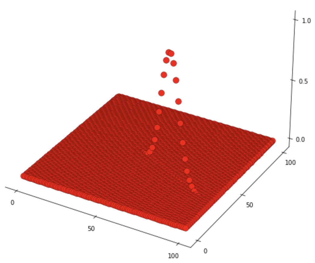
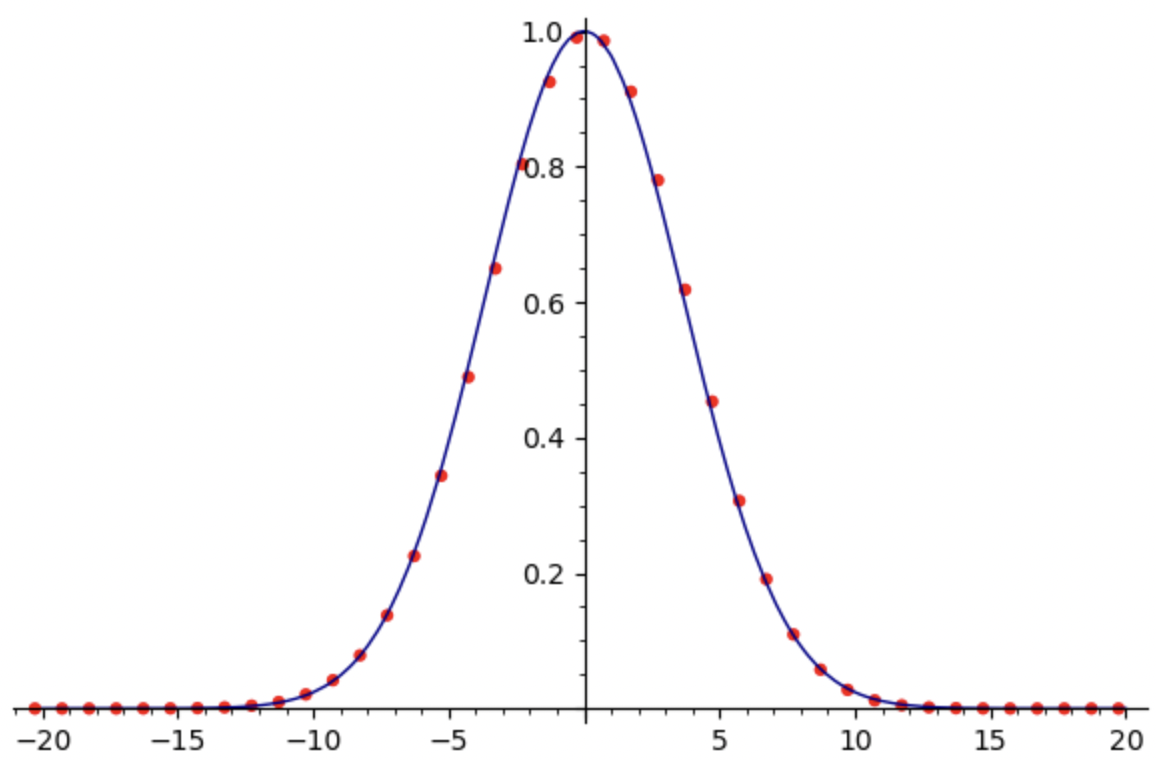
Figure 1: Left: The coefficients of $[t^{150}]F(\mathbf{z},t)$ when $d=1$, divided by the maximum coefficient and shifted to put the maximum at the origin. Right: The coefficients of $[t^{150}]F(1,z_{2},t)$ compared to their limiting normal distribution and shifted to put the maximum at the origin.

Figure 1 shows the problem establishing a limit theorem on the coefficients of $F(\mathbf{z},t)$: the coefficients approach a normal distribution, but the distribution is supported on a $d$-dimensional slice of $\mathbb{R}^{d+1}$. Indeed, if the size $n$ of one of our restricted permutations is fixed and the number $i_{k}$ of $k$ cycles it contains is specified for all $k\geq 2$ then its number of one cycles (i.e., fixed points) is uniquely determined as $i_{1}=n-2i_{2}-\cdots-(d+1)i_{d+1}$. We thus establish Conjecture 3 by setting $z_{1}=1$ and applying the techniques of ACSV to the coefficients of $F(1,z_{2},\dots,z_{d},t)$.

Theorem 4.

Let $h(t)=1-t-\cdots-t^{d+1}$ and let $\rho>0$ be the smallest positive root of $h(t)$. As $n\rightarrow\infty$, the maximum coefficient of $[t^{n}]F(\mathbf{z},t)$ as a polynomial in $z_{2},\dots,z_{d+1}$ approaches

$$A_{n}=\frac{\rho^{-n}n^{-d/2}}{-\rho h^{\prime}(\rho)(2\pi)^{d/2}}\sqrt{\frac{(1+2\rho+\dots+(d+1)\rho^{d})^{d+2}}{(1+\rho+\dots+\rho^{d})\rho^{\frac{d(d+1)}{2}}}}.$$

Furthermore,

$$\sup_{s_{2},\dots,s_{d+1}\in\mathbb{N}}\left|\frac{[z^{s_{2}}_{2}\cdots z^{s_{d+1}}_{d+1}t^{n}]F(1,z_{2},\dots,z_{d+1},t)}{A_{n}}-v_{n}(s_{2},\dots,s_{d+1})\right|\rightarrow 0$$ (1)

where

• $v_{n}(\mathbf{s})=\exp\left[-\frac{(\mathbf{s}-n\mathbf{m})\mathcal{H}^{-1}(\mathbf{s}-n\mathbf{m})^{T}}{2n}\right]$,

• $\mathbf{m}=\left(-\frac{\rho^{2}}{h^{\prime}(\rho)},\ldots,-\frac{\rho^{d+1}}{h^{\prime}(\rho)}\right)$,

• and $\mathcal{H}$ is the non-singular matrix with entries

  $$\mathcal{H}_{i,j}=\begin{cases}\frac{\rho^{i+j+1}h^{\prime\prime}(\rho)-\rho^{i+j}(1+i+j)h^{\prime}(\rho)}{h^{\prime}(\rho)^{3}}&i\neq j\\[5.69054pt] \frac{\rho^{i+j+1}h^{\prime\prime}(\rho)-\rho^{i+j}(1+i+j)h^{\prime}(\rho)-\rho^{i}h^{\prime}(\rho)^{2}}{h^{\prime}(\rho)^{3}}&i=j\end{cases}\;.$$

1.2 Main Theorem

As noted above, while proving Theorem 4 we realized that our approach could be generalized to cover other results in the literature.

Theorem 5 (Main Theorem).

Let $F(\mathbf{z},t)=\frac{G(\mathbf{z},t)}{H(\mathbf{z},t)}$ be a ratio of functions where

$$H(\mathbf{z},t)=1-q(t)-\sum_{k=1}^{d}q_{k}(t)z_{k},$$

let $P(t)=H(\mathbf{1},t)$, and let $\rho$ be the smallest positive root of $P(t)$. Suppose that

• each of the $q_{i}(t)$ is a non-zero polynomial vanishing at the origin and $q(t)$ is a complex-valued analytic function for $|t|\leq\rho$ that vanishes at the origin,

• the power series expansion of $S(\mathbf{z},t)=1-H(\mathbf{z},t)=q(t)+\sum_{k}q_{k}(t)z_{k}$ at the origin has non-negative coefficients,

• the exponents appearing in the power series $q(t)$ have greatest common divisor $1$, and

• $G(\mathbf{1},\rho)$ is non-zero.

As $n\rightarrow\infty$, the maximum coefficient of $[t^{n}]F(\mathbf{z},t)$ as a polynomial in $z_{1},\ldots,z_{d}$ approaches

$$A_{n}=\rho^{-n}n^{-d/2}\frac{G(\mathbf{1},\rho)}{-\rho P^{\prime}(\rho)(2\pi)^{d/2}\sqrt{\det\mathcal{H}}},$$

where $\mathcal{H}$ is the non-singular $d\times d$ matrix

$$\mathcal{H}_{i,j}=\begin{cases}\displaystyle\frac{\rho q_{i}(\rho)q_{j}(\rho)P^{\prime\prime}(\rho)-(q_{j}(\rho)q^{\prime}_{i}(\rho)\rho+q_{i}(\rho)q^{\prime}_{j}(\rho)\rho-q_{i}(\rho)q_{j}(\rho))P^{\prime}(\rho)}{\rho^{2}P^{\prime}(\rho)^{3}}&i\neq j\\[11.38109pt] \displaystyle\frac{\rho q_{j}(\rho)^{2}P^{\prime\prime}(\rho)-(2q_{j}(\rho)q^{\prime}_{j}(\rho)\rho-q_{j}(\rho)^{2})P^{\prime}(\rho)-q_{j}(\rho)\rho P^{\prime}(\rho)^{2}}{\rho^{2}P^{\prime}(\rho)^{3}}&i=j\end{cases}\;$$ (2)

whose determinant

$$\det\mathcal{H}=\frac{(-1)^{d}\left(\prod_{k=1}^{d}q_{k}(\rho)\right)\left[(q(\rho)-1)\left(\rho P^{\prime\prime}(\rho)+P^{\prime}(\rho)+\rho\sum_{k=1}^{d}\frac{q^{\prime}_{k}(\rho)^{2}}{q_{k}(\rho)}\right)+q^{\prime}(\rho)^{2}\rho\right]}{P^{\prime}(\rho)^{d+2}\rho^{d+1}}$$ (3)

is non-zero. Furthermore,

$$\sup_{s_{1},\ldots,s_{d}\in\mathbb{N}}\left|\frac{[z_{1}^{s_{1}}\cdots z_{d}^{s_{d}}t^{n}]F(z_{1},\ldots,z_{d},t)}{A_{n}}-v_{n}(s_{1},\ldots,s_{d})\right|\rightarrow 0$$

where

$$v_{n}(\mathbf{s})=\exp\left[-\frac{(\mathbf{s}-n\mathbf{m})\mathcal{H}^{-1}(\mathbf{s}-n\mathbf{m})^{T}}{2n}\right]\quad\text{ for }\quad\mathbf{m}=\left(\frac{-q_{1}(\rho)}{\rho P^{\prime}(\rho)},\ldots,\frac{-q_{d}(\rho)}{\rho P^{\prime}(\rho)}\right).$$

Remark 6.

Although the form of $H$ in Theorem 5 might seem highly restrictive, generating functions of this form appear quite frequently when tracking parameters in combinatorial classes using, for instance, the symbolic method framework described in Flajolet and Sedgewick [8]. Further examples are given in Section 1.3.

Remark 7.

The methods of ACSV still apply when some of the assumptions in Theorem 5 are relaxed. For instance, coefficient non-negativity and coprimality of the exponents appearing in $q(t)$ guarantees which singularity of $F(\mathbf{z},t)$ dictates asymptotic behaviour. If this coprimality fails then multiple singularities can dictate asymptotics, resulting in possibly periodic behaviour (for instance, a central limit theorem holding for even $n$ and all coefficients vanishing for odd $n$). If the power series expansion of $S(\mathbf{z},t)$ at the origin has negative coefficients then it can be difficult (and computationally expensive [15]) to detect which singularities (if any) determine asymptotic behaviour.

Section 2 surveys the basics of ACSV and how it can be used to derive LCLTs, summarized in Figure 2, after which Section 3 applies these techniques to prove Theorem 5.

Figure 2: A schema to prove LCLTs using Proposition 14 below.

1.3 Additional Examples

We now survey some additional applications of Theorem 5.

Strings with Tracked Letters

Let $\mathcal{A}=\{a_{1},\dots,a_{\ell}\}$ be an alphabet with $\ell$ letters and let $\Omega=\{\omega_{1},\dots,\omega_{d}\}\subset\mathcal{A}$ be a subset of $d$ letters we wish to track. The multivariate generating function enumerating such strings is

$$F(\mathbf{z},t)=\frac{1}{1-(z_{1}+z_{2}+\ldots+z_{d})t-(\ell-d)t},$$

which trivially satisfies the hypotheses of Theorem 5 when $\ell>d$ (if $\ell=d$ then all coefficients live in a $d$-dimensional hyperplane of $\mathbb{R}^{d+1}$, because adding the number of occurrences of each letter gives the length of the string). Thus, as $n\rightarrow\infty$, the maximum coefficient of $[t^{n}]F(\mathbf{z},t)$ as a polynomial in $z_{1},\ldots,z_{d}$ approaches

$$A_{n}=\ell^{n}n^{-d/2}\frac{1}{(2\pi)^{d/2}\sqrt{\frac{\ell-d}{\ell^{d+1}}}}$$

and

$$\sup_{s_{1},\ldots,s_{d}\in\mathbb{N}}\left|\frac{[z_{1}^{s_{1}}\cdots z_{d}^{s_{d}}t^{n}]F(z_{1},\ldots,z_{d},t)}{A_{n}}-\exp\left[-\frac{(\mathbf{s}-n\mathbf{m})\mathcal{H}^{-1}(\mathbf{s}-n\mathbf{m})^{T}}{2n}\right]\right|\rightarrow 0,$$

where $\mathbf{m}=\left(\frac{1}{\ell},\ldots,\frac{1}{\ell}\right)$ and $\mathcal{H}$ is the non-singular $d\times d$ matrix with off-diagonal entries $-\frac{1}{\ell^{2}}$ and diagonal entries $\frac{\ell-1}{\ell^{2}}$. Note that tracking the number of $1$s in binary strings (where $\ell=2$ and $d=1$) recovers the classical central limit theorem,

$$\binom{n}{s}=[z^{s}t^{n}]\frac{1}{1-(1+z)t}\approx 2^{n}\sqrt{\frac{2}{\pi n}}e^{-(n-2s)^{2}/2n}.$$

Compositions with Tracked Summands

Fix a positive integer $d$ and recall that an (integer) composition of size $n$ is an ordered tuple of positive integers which sum to $n$. If $\mathcal{C}$ is the class of compositions, enumerated by size and the number of times each element of $\{1,\dots,d\}$ occurs, then $\mathcal{C}$ has the multivariate generating function

$$\mathcal{C}(\mathbf{z},t)=\frac{1}{1-S(\mathbf{z},t)}=\frac{1}{1-z_{1}t-z_{2}t^{2}-\cdots-z_{d}t^{d}-\frac{t^{d+1}}{1-t}},$$

where

$$S(\mathbf{z},t) =z_{1}t+z_{2}t^{2}+\cdots+z_{d}t^{d}+\sum_{k\geq d+1}t^{k}$$

$$=z_{1}t+z_{2}t^{2}+\cdots+z_{d}t^{d}+\frac{t^{d+1}}{1-t}$$

is the multivariate generating function of positive integers where $z_{k}$ tracks the number of occurrences of $k$. Once again, it is easy to verify the hypotheses of Theorem 5 hold with $\rho=1/2$ the smallest positive root of $P(t)=H(\mathbf{1},t)=1-\frac{t}{1-t}$. Figure 3 illustrates the corresponding local central limit theorem when $d=1$ and $d=2$.

Theorem 8.

As $n\rightarrow\infty$ the maximum coefficient of $[t^{n}]C(\mathbf{z},t)$ as a polynomial in $z_{1},\dots,z_{d}$ approaches

$$A_{n}=2^{n}n^{-d/2}\frac{2^{\frac{d^{2}}{4}+\frac{7d}{4}+1}}{2(2\pi)^{d/2}\sqrt{(d^{2}+4d+6)2^{d}-2}},$$

and

$$\sup_{s_{1},\dots,s_{d}\in\mathbb{N}}\left|\frac{[z^{s_{1}}_{1}\cdots z^{s_{d}}_{d}t^{n}]\mathcal{C}(z_{1},\dots,z_{d},t)}{A_{n}}-\exp\left[-\frac{(\mathbf{s}-n\mathbf{m})\mathcal{H}^{-1}(\mathbf{s}-n\mathbf{m})^{T}}{2n}\right]\right|\rightarrow 0$$

where $\mathbf{m}=\left(\frac{1}{4},\frac{1}{8},\ldots,\frac{1}{2^{d+1}}\right)$ and $\mathcal{H}$ is the $d\times d$ matrix with off-diagonal entries $\mathcal{H}_{i,j}=-2^{-i-j-2}(i+j-3)$ and diagonal entries $\mathcal{H}_{j,j}=2^{-2(j+1)}(2^{j+1}-2j+3)$.

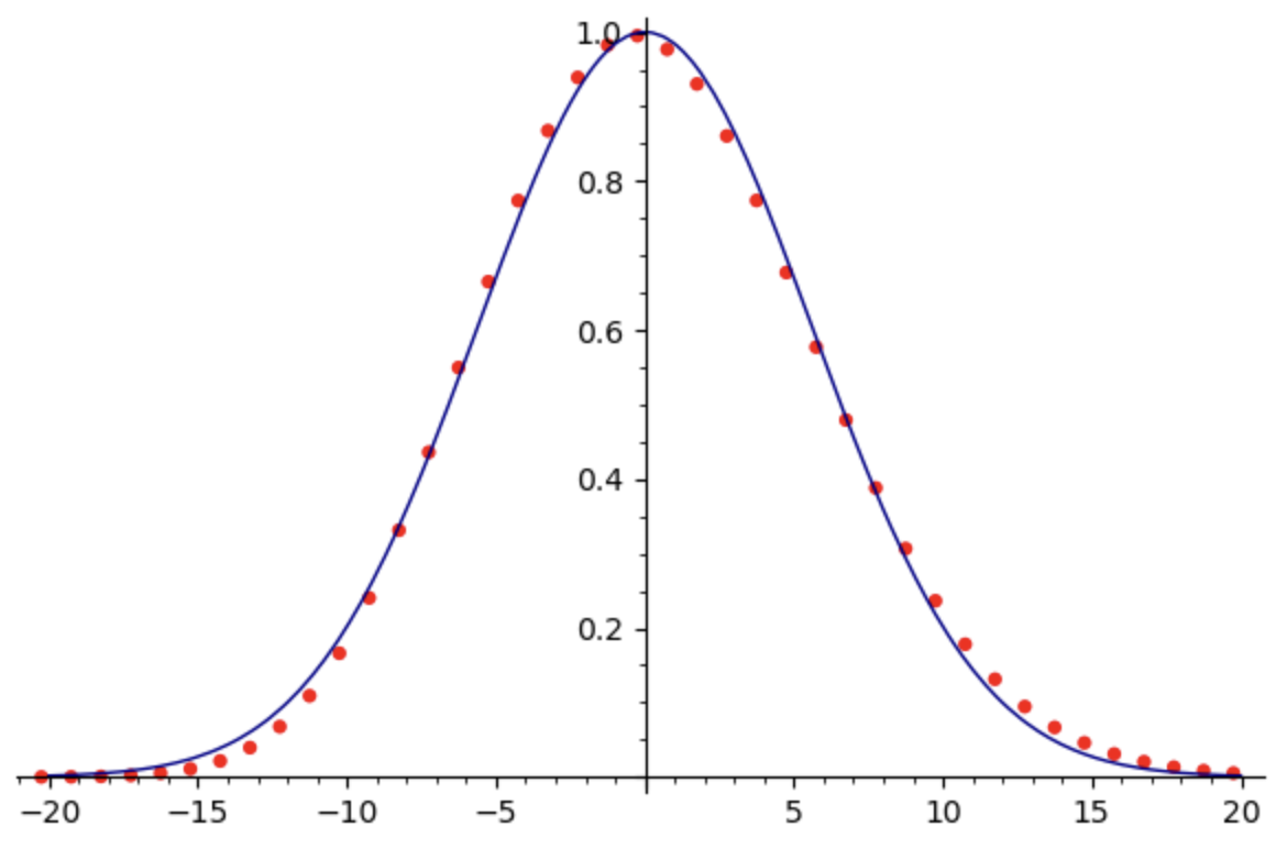
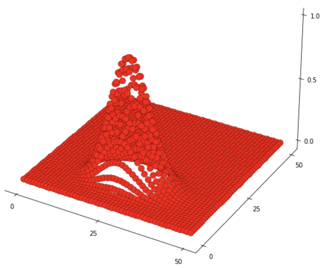
Figure 3: Left: The coefficients of $[t^{100}]\frac{1}{1-z_{1}t-\frac{t^{2}}{1-t}}$ divided by the projected maximum coefficient compared to their limiting normal distribution and shifted to put the maximum at the origin. Right: The coefficients of $[t^{100}]\frac{1}{1-z_{1}t-z_{2}t^{2}-\frac{t^{3}}{1-t}}$, divided by the projected maximum coefficient and shifted to put the maximum at the origin.

The flexibility of Theorem 5 allows us to modify the restrictions on the elements appearing or tracked among the compositions under consideration. For instance, for any finite set $\Omega\subset\mathbb{Z}_{>0}$ the multivariate generating function enumerating compositions by size and number of times each element of $\Omega=\{\omega_{1},\dots,\omega_{d}\}$ occurs is

$$F(\mathbf{z},t)=\frac{1}{1-\sum_{k=1}^{d}(z_{k}-1)t^{\omega_{k}}-\frac{t}{1-t}},$$

where $z_{k}$ tracks the number of occurrences of $\omega_{k}$. The hypotheses of Theorem 5 still hold, so a local central limit theorem applies (although, of course, the parameters of the limiting distribution will depend on which summands are tracked).

Even more generally, we can restrict our compositions to summands in some set $\Lambda\subset\mathbb{Z}_{>0}$ and track occurrences of elements in a finite subset $\Omega=\{\omega_{1},\dots,\omega_{d}\}\subset\Lambda$. The relevant multivariate generating function becomes

$$F(\mathbf{z},t)=\frac{1}{1-\sum_{k=1}^{d}(z_{k}-1)t^{\omega_{k}}-\sum_{k\in\Omega}t^{k}}.$$

When the elements of $\Omega$ are coprime, Theorem 5 applies, so a local central limit theorem holds (when the elements of $\Omega$ have greatest common divisor larger than $1$ then some intervention is needed to determine which singularities determine asymptotic behaviour).

Remark 9.

Restricting compositions to use only the numbers $1,\dots,d+1$ and tracking occurrences of those numbers gives the same generating function as the family of restricted permutations discussed above, whose behaviour is described in Theorem 4.

$n$-Colour Compositions with Tracked Summands

Finally, we consider the class of $n$-colour compositions, introduced by Agarwal [1] and studied in Gibson et al. [10], where each integer $i$ is coloured by one of $i$ available colours (each summand must be coloured and different colourings give distinct $n$-colour compositions).

Example 10.

The twenty-one $n$-colour compositions of 4 are

$$4_{1},\text{ }4_{2},\text{ }4_{3},\text{ }4_{4},$$

$$3_{1}1_{1},\text{ }3_{2}1_{1},\text{ }3_{3}1_{1},\text{ }1_{1}3_{1},\text{ }1_{1}3_{2},\text{ }1_{1}3_{3},$$

$$2_{1}2_{1},\text{ }2_{1}2_{2},\text{ }2_{2}2_{1},\text{ }2_{2}2_{2},$$

$$2_{1}1_{1}1_{1},\text{ }2_{2}1_{1}1_{1},\text{ }1_{1}2_{1}1_{1},\text{ }1_{1}2_{2}1_{1},\text{ }1_{1}1_{1}2_{1},\text{ }1_{1}1_{1}2_{2},$$

$$1_{1}1_{1}1_{1}1_{1},$$

where the subscripts denote the colours assigned to each summand.

Once again, we fix a positive integer $d$ and track the number of times each element of $\{1,\dots,d\}$ occurs. If $\mathcal{S}_{n}$ is the class of positive integers where each integer $i$ is coloured with one of $i$ possible colours then

$$\mathcal{S}_{n}(\mathbf{z},t) =z_{1}t+2z_{2}t^{2}+\cdots+dz_{d}t^{d}+(d+1)t^{d+1}+(d+2)t^{d+2}+\cdots$$

$$=z_{1}t+2z_{2}t^{2}+\cdots+dz_{d}t^{d}+t\frac{d}{dt}\left(\frac{t^{d+1}}{1-t}\right)$$

$$=z_{1}t+2z_{2}t^{2}+\cdots+dz_{d}t^{d}+\frac{dt^{d+1}}{1-t}+\frac{t^{d+1}}{(1-t)^{2}}$$

is the multivariate generating function of positive integers where $z_{k}$ tracks the number of occurrences of $k$, so the corresponding multivariate generating function for $n$-colour compositions is

$$C_{n}(\mathbf{z},t)=\frac{1}{1-z_{1}t-2z_{2}t^{2}-\cdots-dz_{d}t^{d}-\frac{dt^{d+1}}{1-t}-\frac{t^{d+1}}{(1-t)^{2}}}.$$

As expected, the hypotheses of Theorem 5 hold, and we get a (messier) LCLT whose parameters are given explicitly in the Sage notebook corresponding to this paper. Similar to our last example, we may further restrict which elements (or colours!) are allowed or tracked, and immediately get LCLTs. The proofs for such extensions follow similarly to those for integer compositions.

1.4 Past Work

Limit theorems have a long history in combinatorics and probability theory, dating back to their origins in eighteenth century work of de Moivre and Laplace, and classical treatments can be found in most standard probability textbooks [7, 6]. The systematic use of bivariate generating functions to establish limit theorems is now a well-established part of the theory of analytic combinatorics: see Flajolet and Sedgewick [8, Chapter IX] for an introduction, and Hwang [12] for a list of more than 25 limit laws proven by the late Philippe Flajolet using this framework, including patterns in words, cost analyses of various sorting algorithms, parameters in different kinds of trees, polynomials with restricted coefficients, and ball-urn models.

A series of papers by Bender [2], Bender and Richmond [3, 4], and Richmond and Gao [9], proved central limit theorems for multivariate generating functions under certain assumptions on their singular sets that were usually verified in an ad-hoc manner. Over the last twenty years, a theory of analytic combinatorics in several variables [14, 16] has been developed by Pemantle, Wilson, Baryshnikov, Melczer, and collaborators, to give more systematic methods for the asymptotics of multivariate generating functions; our results are based around these techniques. We also note that this work began concurrently with the publication of the textbook [14] of the first author (which includes details on how to computationally prove the specific example of (1) for fixed – not arbitrary – dimension, and does not include our main Theorem 5).

2 Background on ACSV and Limit Theorems

Let $F(\mathbf{z},t)=G(\mathbf{z},t)/H(\mathbf{z},t)$ be a ratio of complex-valued functions $G$ and $H$ analytic in a sufficiently large domain $\mathcal{D}\subset\mathbb{C}^{2}$, and suppose that $F$ has a power series expansion

$$F(\mathbf{z},t)=\sum_{(\mathbf{i},k)\in\mathbb{N}^{d+1}}f_{\mathbf{i},k}\mathbf{z}^{\mathbf{i}}t^{k}=\sum_{(\mathbf{i},k)\in\mathbb{N}^{d+1}}f_{i_{1},\dots,i_{d},k}z_{1}^{i_{1}}\cdots z_{d}^{i_{d}}t^{k}$$

valid in some neighbourhood of the origin (meaning $H(0)\neq 0$). To derive limit theorems we study the asymptotic behaviour of coefficients $(f_{\mathbf{r},n})_{\mathbf{r}\in\mathbb{N}^{d}}$ as $n\rightarrow\infty$. We focus on the case when the numerator $G$ is a polynomial, and assume throughout that $H$ is not a constant to avoid the trivial case when $F$ is a polynomial.

Remark 11.

There are several natural ways to take the sequence indices of $f_{\mathbf{i},k}$ to infinity and search for limit theorems: for instance, one could examine the terms with $i_{1}+\cdots+i_{d}+k=n$ and take $n\rightarrow\infty$. For us it makes the most combinatorial sense to take the final index (encoding permutation or composition size in our examples) to infinity and study coefficient behaviour as the first $d$ indices (encoding cycle or composition structure) vary.

Asymptotic arguments typically start with the Cauchy integral representation

$$f_{\mathbf{r},n}=\frac{1}{(2\pi i)^{d+1}}\int_{\mathcal{T}}F(\mathbf{z},t)\mathbf{z}^{-\mathbf{r}}t^{-n}\frac{d\mathbf{z}dt}{z_{1}\cdots z_{d}t},$$ (4)

where $\mathcal{T}$ is any product of circles $|z_{j}|=|t|=\varepsilon$ sufficiently close to the origin. The methods of ACSV manipulate the domain of integration $\mathcal{T}$ to convert the Cauchy integral (4) into something that can be asymptotically approximated. As in the more classical univariate case, this process depends heavily on the singular set of the generating function $F$. Because $F$ is a ratio, its singularities form a subset of the analytic variety $\mathcal{V}=\{(\mathbf{z},t)\in\mathbb{C}^{d+1}:H(\mathbf{z},t)=0\}$ defined by the vanishing of the denominator $H$.

Univariate meromorphic functions always have a finite set of dominant singularities dictating asymptotic behaviour, and explicit expressions for their coefficient asymptotics can be determined by adding up contributions given by each such point. In contrast, in dimension $d\geq 2$ the set $\mathcal{V}$ is infinite, and the geometry of $\mathcal{V}$ plays a large role. The simplest case, and the only one we need to consider in this paper, occurs when $H$ and its partial derivatives don’t simultaneous vanish at any point (which makes $\mathcal{V}$ a complex manifold). Two types of singularities turn out to be crucial to the analysis.

Definition 12.

Let $(\mathbf{w},s)\in\mathbb{C}_{*}^{d+1}=(\mathbb{C}\setminus\{0\})^{d+1}$. We say that $(\mathbf{w},s)$ is

• a minimal point if $H(\mathbf{w},s)=0$ and there is no element of $\mathcal{V}$ which is coordinate-wise closer to the origin, i.e., there does not exist $(\mathbf{y},q)$ with $|y_{j}|<|w_{j}|$ for all $1\leq j\leq d$ and $|q|<|s|$ such that $H(\mathbf{y},q)=0$;

• a strictly minimal point if it is minimal and no other point of $\mathcal{V}$ has the same coordinate-wise modulus;

• a finitely minimal point if it is minimal and only a finite number of points in $\mathcal{V}$ have the same coordinate-wise modulus;

• a smooth critical point in the direction $(\mathbf{r},1)\in\mathbb{R}_{>0}^{d+1}$ if it satisfies the system of equations

  $$H(\mathbf{w},t)=0,\qquad\frac{w_{1}}{r_{1}}H_{z_{1}}(\mathbf{w},s)=\frac{w_{2}}{r_{2}}H_{z_{2}}(\mathbf{w},s)=\cdots=\frac{w_{d}}{r_{d}}H_{z_{d}}(\mathbf{w},s)=tH_{t}(\mathbf{w},s)$$ (5)

  and one of these partial derivatives does not vanish (which, in fact, implies that all of the derivatives do not vanish).

Very roughly, in the smooth setting one can push out the domain of integration $\mathcal{T}$ in (4) to approach the set of singularities, take a residue in one variable to reduce to a $d-1$ dimensional integral lying ‘on the singular set,’ and then (hopefully) determine asymptotics of this lower dimensional integral using the saddle-point method. Minimal points are those to which $\mathcal{T}$ can be easily deformed, while critical points are those where it may be possible to perform a saddle-point analysis after computing a residue. In order to compute the desired saddle-point approximation, one must also verify the non-singularity of a matrix arising in the computation.

Definition 13.

Let $(\mathbf{w},s)\in\mathbb{C}_{*}^{d+1}$ be a smooth critical point in the direction $(\mathbf{r},1)$ and suppose $H_{t}(\mathbf{w},s)\neq 0$. The phase Hessian of $H$ at $(\mathbf{z},t)=(\mathbf{w},s)$ is the $d\times d$ matrix $\mathcal{H}$ with entries

$$\mathcal{H}_{i,j}=\begin{cases}r_{i}r_{j}+U_{i,j}-r_{j}U_{i,d+1}-r_{i}U_{j,d+1}+r_{i}r_{j}U_{d+1,d+1}&:i\neq j\\[8.53581pt] r_{i}+r_{i}^{2}+U_{i,i}-2r_{i}U_{i,d+1}+r_{i}^{2}U_{d+1,d+1}&:i=j\end{cases}$$ (6)

where $U_{i,j}=\frac{w_{i}w_{j}H_{z_{i}z_{j}}(\mathbf{w},s)}{tH_{t}(\mathbf{w},s)}$ for $1\leq i,j\leq d,$ while $U_{i,d+1}=\frac{w_{i}H_{z_{i}t}(\mathbf{w},s)}{H_{t}(\mathbf{w},s)}$ and $U_{d+1,d+1}=\frac{tH_{tt}(\mathbf{w},s)}{H_{t}(\mathbf{w},s)}$.

Chapter 5 of Melczer [14] shows how the argument sketched above can be used to derive asymptotics of multivariate rational functions with finitely minimal critical points whose phase Hessian matrices are nonsingular. The asymptotic results presented in that chapter vary smoothly with the direction $\mathbf{r}$ under small perturbations, which allows for the derivation of LCLTs.

Proposition 14 (Melczer [14, Proposition 5.10]).

Suppose $F(\mathbf{z},t)=G(\mathbf{z},t)/H(\mathbf{z},t)$ has a power series expansion $F(\mathbf{z},t)=\sum_{(\mathbf{i},k)\in\mathbb{N}^{d+1}}f_{\mathbf{i},k}\mathbf{z}^{\mathbf{i}}t^{k}$ at the origin such that $f_{\mathbf{i},k}$ is non-negative for all but a finite number of terms. Suppose further that, in some direction $(\mathbf{m},1)$, there is a strictly minimal critical point of the form $(\mathbf{1},\rho)$ for some $\rho>0$. If $H_{t}(\mathbf{w},\rho)$ and $G(\mathbf{w},\rho)$ are non-zero, and the phase Hessian $\mathcal{H}$ of $H$ at $(\mathbf{1},\rho)$ is nonsingular, then

$$\sup_{\mathbf{s}\in\mathbb{Z}^{d}}n^{d/2}\left|\rho^{n}f_{\mathbf{s},n}-\frac{-G(\mathbf{1},\rho)}{\rho H_{t}(\mathbf{1},\rho)}\frac{(2\pi n)^{-d/2}}{\sqrt{\det\mathcal{H}}}\exp\left[-\frac{(\mathbf{s}-n\hat{\mathbf{m}})^{T}\mathcal{H}^{-1}(\mathbf{s}-n\hat{\mathbf{m}})}{2n}\right]\right|\rightarrow 0.$$ (7)

Remark 15.

Proposition 5.10 in Melczer [14] requires $G$ and $H$ to be polynomials to simplify its presentation, however the result continues to hold for analytic functions [14, Remark 5.14].

The critical point equations (5) consist of $d+1$ equations in $d+1$ variables, and generically have a finite set of solutions. Determining which points are critical, an algebraic condition, is usually (much) easier than determining minimality, which is a semi-algebraic condition involving inequalities among the moduli of coordinates. Thus, most algorithms to determine sequence asymptotics using ACSV fix a direction, compute critical points in this direction, and then study the critical points to determine which are minimal points. In contrast, because Proposition 14 requires a minimal critical point of the form $(\mathbf{1},t)$, to prove an LCLT it is often easiest to use (5) to discover a direction $\mathbf{r}=(\mathbf{m},1)$ with critical points of this form and then verify the required conditions. This leads to the approach summarized in Figure 2 above.

Determining minimality is easier for points with positive coefficients when $F(\mathbf{z})$ has only a finite number of non-negative coefficients, as it does under our assumptions. The following result should be seen as a multivariate generalization of the well-known Vivanti-Prinsheim theorem in the univariate case.

Lemma 16 (Melczer [14, Lemma 5.7]).

Suppose $F(\mathbf{z},t)=G(\mathbf{z},t)/H(\mathbf{z},t)$ has a power series expansion at the origin with (at most) a finite number of negative coefficients. Then $(\mathbf{w},\rho)\in\mathbb{R}_{>0}^{d}$ is minimal if the line segment from the origin to $(\mathbf{w},\rho)$ contains no roots of $H(\mathbf{z},t)$, i.e., if

$$H(sw_{1},\dots,sw_{d},s\rho)\neq 0\text{ for all }s\in(0,1).$$

The final proposition we present offers a method of proving that the minimal critical point of the form $(\mathbf{1},t)$ is indeed strictly minimal. To introduce the proposition, we first give the following definition.

Definition 17 (Melczer [14, Definition 5.9]).

A power series $S(\mathbf{z})=\sum_{\mathbf{n}\in\mathbb{N}^{d}}p_{\mathbf{n}}\mathbf{z}^{\mathbf{n}}$ is called aperiodic if every element of $\mathbb{Z}^{d}$ can be written as an integer linear combination of the exponents $\{\mathbf{n}\in\mathbb{N}^{d}:p_{\mathbf{n}}\neq 0\}$ appearing in $S$.

Proposition 18 (Based on Melczer [14, Proposition 5.5]).

Suppose $F(\mathbf{z})=G(\mathbf{z})/H(\mathbf{z})$ is a ratio of functions $G$ and $H$. If $H(\mathbf{z})=1-S(\mathbf{z})$ for some aperiodic power series $S$ with non-negative coefficients then every minimal point that is within the domain of convergence of the power series expansion of $F(\mathbf{z})$ is strictly minimal and has positive real coordinates.

Proof.

Suppose that $\mathbf{w}$ is a minimal point and for each $1\leq j\leq d$ write $w_{j}=x_{j}e^{i\theta_{j}}$ with $x_{j}>0$ and $\theta_{j}\in\mathbb{R}$. Let $s_{\mathbf{n}}$ denote the coefficient of $z^{\mathbf{n}}$ in $S(\mathbf{z})$. Then

$$1=|S(\mathbf{w})|=\left|\sum_{\mathbf{n}\in\mathbb{N}^{d}}s_{\mathbf{n}}\mathbf{x}^{\mathbf{n}}e^{i(\mathbf{n}\theta)}\right|\leq\sum_{\mathbf{n}\in\mathbb{N}^{d}}s_{\mathbf{n}}\mathbf{x}^{\mathbf{n}}$$

since $\mathbf{w}$ is within the domain of convergence of $G$ and $H$ and hence $|S(\mathbf{w})|\leq S(|w_{1}|,\ldots,|w_{d}|)$. ∎

With this background out of the way, we are now ready to prove Theorem 5 and consequently the applications discussed above.

3 Proof of Theorem 5

Assume that the hypotheses of Theorem 5 hold.

Step 1: Finding the correct direction.

Following the outline of Figure 2, we substitute $\mathbf{w}=(\mathbf{1},\rho)$ into the smooth critical point equations (5) to find that $\mathbf{w}$ is a critical point in the direction $(\mathbf{m},1)$ where

$$\mathbf{m}=\left(\frac{-q_{1}(\rho)}{\rho P^{\prime}(\rho)},\dots,\frac{-q_{d}(\rho)}{\rho P^{\prime}(\rho)}\right).$$

Step 2: Establishing strict minimality.

Suppose $H(s,\ldots,s,t)=0$ for $0<s<1$ and $0<t<\rho$. Then $s\sum_{k=1}^{d}q_{k}(t)=1-q(t)$ and we cannot have $\sum_{k=1}^{d}q_{k}(t)=0$, since then $q(0)=1$ which would violate the fact that $q$ has no constant, so

$$s=\frac{1-q(t)}{\sum_{k=1}^{d}q_{k}(t)}.$$

Our assumptions imply that the polynomial $\sum_{k=1}^{d}q_{k}(t)$ and series expansion of $q(t)$ have non-negative coefficients, and $0<q(\rho)<1$, so that $|s|$ increases as $0<t<\rho$ decreases. Thus $H(s,\ldots,s,s\rho)\neq 0$ for all $0<s<1$, and $\mathbf{w}$ is minimal by applying Lemma 16 to the function $1/H(\mathbf{z},t)=1/(1-S(\mathbf{z},t))$ whose series expansion at the origin has non-negative coefficients. In fact, our assumptions imply that $S(\mathbf{z},t)$ is an aperiodic power series with non-negative coefficients, so Proposition 18 implies that $\mathbf{w}$ is a strictly minimal critical point.

Step 3a: Computing an $LU$-factorization.

We now prove that the phase Hessian matrix defined by (6), which simplifies to (2) in our case, has non-zero determinant. To compute this symbolic determinant, we originally used the Sage computer algebra system to compute and factor the Hessian determinant for the permutation generating function described by Proposition 2 in small dimensions. Observing a pattern in the factors, we were able to conjecture, and then a posteriori prove, an $LU$-factorization for the Hessian matrix in this case, and then extend to the general case. This approach immediately gives the Hessian determinant: if $\mathcal{H}U=L$ for a lower triangular matrix $L$ and an upper triangular matrix $U$ with diagonal elements equal to 1 then $\det\mathcal{H}$ is simply the product of the diagonal elements of $L$.

Remark 19.

When the dimension $d$ is fixed, the matrix equation $\mathcal{H}U=L$ defines an explicit system of equations in terms of the entries of $U$ and $L$, so it is often possible to computationally determine suitable $U$ and $L$ in low dimension, conjecture their general form, then prove this inference. This approach to symbolic determinants is described in the well-known treatise of Krattenthaler [13], which attributes the popularization of such a ‘guess-and-check’ $LU$-factorization to George Andrews after he used it to great effect in a variety of papers starting in the 1970s.

Our companion Sage notebook to this paper gives a procedure to calculate $U$ and $L$ for any fixed $d$. Studying the numerator and denominator of the rational function entries we are able to deduce certain patterns, such as the denominators being constant down columns, which leads us to conjecture that in general dimension $\mathcal{H}U=L$ where
$$\text{U}_{ij}=\begin{cases}\frac{q_{j}(\rho)g_{ij}}{r_{j}}&i<j\\[2.84526pt] 1&i=j\\[2.84526pt] 0&i>j\end{cases}$$ and $$L_{ij}=\begin{cases}0&i<j\\[2.84526pt] \frac{-q_{j}(\rho)r_{j+1}}{P^{\prime}(\rho)\rho r_{j}}&i=j\\[2.84526pt] \frac{q_{j}(\rho)q_{i}(\rho)s_{ij}}{P^{\prime}(\rho)\rho r_{j}}&i>j\end{cases}$$

for

$$r_{j} =P^{\prime}(\rho)^{2}\rho-P^{\prime\prime}(\rho)\rho A_{j}+2P^{\prime}(\rho)\rho B_{j}-P^{\prime}(\rho)A_{j}-\rho\left(A_{j}D_{j}-B_{j}^{2}\right)$$

$$g_{ij} =P^{\prime}(\rho)+P^{\prime\prime}(\rho)\rho-\rho\left(\frac{q^{\prime}_{i}(\rho)}{q_{i}(\rho)}+\frac{q^{\prime}_{j}(\rho)}{q_{j}(\rho)}\right)\left(P^{\prime}(\rho)+B_{j}-q^{\prime}_{i}(\rho)\right)+\rho\left(D_{j}-\frac{q^{\prime}_{i}(\rho)^{2}}{q_{i}(\rho)}\right)+\frac{\rho q^{\prime}_{i}(\rho)q^{\prime}_{j}(\rho)}{q_{i}(\rho)q_{j}(\rho)}\left(A_{j}-q_{i}(\rho)\right)$$

$$s_{ij} =P^{\prime\prime}(\rho)\rho+\rho D_{j}-\rho\left(\frac{q^{\prime}_{i}(\rho)}{q_{i}(\rho)}+\frac{q^{\prime}_{j}(\rho)}{q_{j}(\rho)}\right)\left(P^{\prime}(\rho)+B_{j}\right)+P^{\prime}(\rho)+\left(\frac{\rho q^{\prime}_{i}(\rho)q^{\prime}_{j}(\rho)}{q_{i}(\rho)q_{j}(\rho)}\right)A_{j}$$

with

$$A_{j}=\sum_{k=1}^{j-1}q_{k}(\rho),\qquad B_{j}=\sum_{k=1}^{j-1}q^{\prime}_{k}(\rho),\qquad C_{j}=\sum_{k=1}^{j-1}q^{\prime}_{k}(\rho)^{2},\qquad D_{j}=\sum_{k=1}^{j-1}\frac{q_{k}^{\prime}(\rho)^{2}}{q_{k}(\rho)}.$$

Although these formulas are quite involved, we note that, by keeping $P^{\prime}(\rho)$ and $P^{\prime\prime}(\rho)$ as symbolic parameters, the entries of $U$ and $L$ are independent of $d$ which allows us to algorithmically verify that $\mathcal{H}U=L$ with the aid a computer algebra system.

We break this verification into into three cases depending on the behaviour of the entries of $U$ and $L$: see Figure 4 for an illustration of the different cases on a $4\times 4$ matrix.

Figure 4: The three cases, distinguished by colour, for $d=4$.

=

Case 1: $j>i$

Case 1: $j>i$

As $U$ is upper-triangular, we have

$$(\mathcal{H}U)_{ij}=\sum_{a=1}^{j}\mathcal{H}_{ia}U_{aj}=\sum_{\begin{subarray}{c}1\leq a<j\\ a\neq i\end{subarray}}\mathcal{H}_{ia}U_{aj}+\mathcal{H}_{ii}U_{ij}+\mathcal{H}_{ij},$$

where we may split the sum in such a way that the summands in the indefinite series have a uniform definition. Using Sage for algebraic manipulations, we see that

$$\mathcal{H}_{ia}U_{aj}=\frac{\alpha_{ij}\left(\frac{q^{\prime}_{a}(\rho)^{2}}{q_{a}(\rho)}\right)+\beta_{ij}q_{a}(\rho)+\gamma_{ij}q^{\prime}_{a}(\rho)}{\rho^{2}P^{\prime}(\rho)^{3}r_{j}}$$

where

$$\alpha_{ij} =\left(P^{\prime}(\rho)q_{j}(\rho)-q^{\prime}_{j}(\rho)A_{j}+q_{j}(\rho)B_{j}\right)P^{\prime}(\rho)q_{i}(\rho)\rho^{2}$$ (8)

$$\beta_{ij} ={\Big{[}}P^{\prime}(\rho)\left(q^{\prime}_{j}(\rho)\rho-q_{j}(\rho)\right)-P^{\prime\prime}(\rho)q_{j}(\rho)\rho+q^{\prime}_{j}(\rho)\rho B_{j}-q_{j}(\rho)\rho D_{j}{\Big{]}}$$ (9)

$$\hskip 14.45377pt\cdot{\Big{[}}(P^{\prime}(\rho)\left(q^{\prime}_{i}(\rho)\rho-q_{i}(\rho)\right)-P^{\prime\prime}(\rho)q_{i}(\rho)\rho{\Big{]}}$$

and

$$\begin{split}\gamma_{ij}=&{\Big{[}}q^{\prime}_{j}(\rho)q_{i}(\rho)+q^{\prime}_{i}(\rho)q_{j}(\rho){\Big{]}}\rho^{2}P^{\prime}(\rho)^{2}-2{\Big{[}}P^{\prime}(\rho)+P^{\prime\prime}(\rho)\rho{\Big{]}}\rho P^{\prime}(\rho)q_{i}(\rho)q_{j}(\rho)\\[5.69054pt] &+{\Big{[}}P^{\prime\prime}(\rho)q^{\prime}_{j}(\rho)q_{i}(\rho)\rho-P^{\prime}(\rho)q^{\prime}_{i}(\rho)q^{\prime}_{j}(\rho)\rho+P^{\prime}(\rho)q^{\prime}_{j}(\rho)q_{i}(\rho){\Big{]}}\rho A_{j}\\[5.69054pt] &+{\Big{[}}q^{\prime}_{j}(\rho)q_{i}(\rho)\rho+q^{\prime}_{i}(\rho)q_{j}(\rho)\rho-q_{i}(\rho)q_{j}(\rho){\Big{]}}\rho P^{\prime}(\rho)B_{j}-P^{\prime\prime}(\rho)q_{i}(\rho)q_{j}(\rho)\rho^{2}B_{j}\\[5.69054pt] &-P^{\prime}(\rho)q_{i}(\rho)q_{j}(\rho)\rho^{2}D_{j}.\end{split}$$ (10)

Since $\alpha_{ij}$, $\beta_{ij}$, $\gamma_{ij},$ and the denominator in our above expression for $\mathcal{H}_{ia}U_{aj}$ are not dependent on $a$,

$$\sum_{\begin{subarray}{c}1\leq a<j\\ a\neq i\end{subarray}}\mathcal{H}_{ia}U_{aj} =\sum_{\begin{subarray}{c}1\leq a<j\\ a\neq i\end{subarray}}\frac{\alpha_{ij}\left(\frac{q^{\prime}_{a}(\rho)^{2}}{q_{a}(\rho)}\right)+\beta_{ij}q_{a}(\rho)+\gamma_{ij}q^{\prime}_{a}(\rho)}{\rho^{2}P^{\prime}(\rho)^{3}r_{j}}$$

$$=\frac{1}{\rho^{2}P^{\prime}(\rho)^{3}r_{j}}\left[\alpha_{ij}\sum_{\begin{subarray}{c}1\leq a<j\\ a\neq i\end{subarray}}\frac{q^{\prime}_{a}(\rho)^{2}}{q_{a}(\rho)}+\beta_{ij}\sum_{\begin{subarray}{c}1\leq a<j\\ a\neq i\end{subarray}}q_{a}(\rho)+\gamma_{ij}\sum_{\begin{subarray}{c}1\leq a<j\\ a\neq i\end{subarray}}q^{\prime}_{a}(\rho)\right]$$

$$=\frac{1}{\rho^{2}P^{\prime}(\rho)^{3}r_{j}}\left[\alpha_{ij}\left(D_{j}-\frac{q^{\prime}_{i}(\rho)^{2}}{q_{i}(\rho)}\right)+\beta_{ij}\left(A_{j}-q_{i}(\rho)\right)+\gamma_{ij}\left(B_{j}-q^{\prime}_{i}(\rho)\right)\right].$$

Substitution of our above formulas then gives, after some algebraic simplification by Sage, that

$$\sum_{\begin{subarray}{c}1\leq a<j\\ a\neq i\end{subarray}}\mathcal{H}_{ia}U_{aj}+\mathcal{H}_{ii}U_{ij}+\mathcal{H}_{ij}=0$$

in this case, as required.

=

Case 2: $i=j$

Case 2: $i=j$

As with Case 1, since $U$ is upper-triangular we have

$$(\mathcal{H}U)_{jj}=\sum_{a=1}^{d}\mathcal{H}_{ja}U_{aj}=\sum_{a=1}^{j}\mathcal{H}_{ja}U_{aj}=\sum_{a=1}^{j-1}\mathcal{H}_{ja}U_{aj}+\mathcal{H}_{jj},$$

where we separate the case $a=j$ since the entries of $U$ have a different definition on the diagonal and above the diagonal. It is therefore sufficient to prove

$$\sum_{a=1}^{j-1}\mathcal{H}_{ja}U_{aj}+\mathcal{H}_{jj}=L_{jj}$$

using the definitions above. Analogously to Case 1,

$$\mathcal{H}_{ja}U_{aj}=\frac{\alpha_{jj}\left(\frac{q^{\prime}_{a}(\rho)^{2}}{q_{a}(\rho)}\right)+\beta_{jj}q_{a}(\rho)+\gamma_{jj}q^{\prime}_{a}(\rho)}{\rho^{2}P^{\prime}(\rho)^{3}r_{j}}$$

where $\alpha_{jj}$, $\beta_{jj}$ and $\gamma_{jj}$ are defined in (8), (9) and (10) respectively. Since $\alpha_{jj}$, $\beta_{jj}$, $\gamma_{jj},$ and the denominator in this expression for $\mathcal{H}_{ja}U_{aj}$ are not dependent on $a$, we can algebraically simplify to get

$$\sum_{a=1}^{j-1}\mathcal{H}_{ja}U_{aj} =\sum_{a=1}^{j-1}\left[\frac{\alpha_{jj}\left(\frac{q^{\prime}_{a}(\rho)^{2}}{q_{a}(\rho)}\right)+\beta_{jj}q_{a}(\rho)+\gamma_{jj}q^{\prime}_{a}(\rho)}{\rho^{2}P^{\prime}(\rho)^{3}r_{j}}\right]$$

$$=\frac{\alpha_{jj}D_{j}+\beta_{jj}A_{j}+\gamma_{jj}B_{j}}{\rho^{2}P^{\prime}(\rho)^{3}r_{j}}.$$

Substitution of our above formulas then gives, after some algebraic simplification by Sage, that

$$\sum_{a=1}^{j-1}\mathcal{H}_{ja}U_{aj}+\mathcal{H}_{jj}-L_{jj}=0$$

in this case, as desired.

Case 3: $j<i$

At this point, we have proven that $\mathcal{H}U$ is lower-triangular and described its diagonal entries, which gives the desired determinant. Although not needed to establish Theorem 5, for completeness we prove the claimed expression above for the below diagonal entries in our companion Sage notebook.

Step 3b: Computing the Hessian determinant

Our $LU$-factorization expresses the Hessian determinant as the product of the diagonal entries of the lower-triangular matrix $L$. In fact, the form of these diagonal entries causes cancellation of many terms, leading to a relatively compact final answer,

$$\det\mathcal{H}=\prod^{d}_{m=1}L_{mm}=\prod^{d}_{m=1}\frac{-q_{m}(\rho)r_{m+1}}{P^{\prime}(\rho)\rho r_{m}} =\frac{(-1)^{d}\left(\prod_{k=1}^{d}q_{k}(\rho)\right)r_{d+1}}{P^{\prime}(\rho)^{d}\rho^{d}r_{1}}$$

$$=\frac{(-1)^{d}\left(\prod_{k=1}^{d}q_{k}(\rho)\right)r_{d+1}}{P^{\prime}(\rho)^{d+2}\rho^{d+1}}.$$

Furthermore,

$$P(\rho)=1-q(\rho)-\sum_{k=1}^{d}q_{k}(\rho)=0\quad\text{and}\quad P^{\prime}(\rho)=-q^{\prime}(\rho)-\sum_{k=1}^{d}q^{\prime}_{k}(\rho)$$

so that $A_{d+1}=\sum_{k=1}^{d}q_{k}(\rho)=1-q(\rho)$ and $B_{d+1}=\sum_{k=1}^{d}q^{\prime}_{k}(\rho)=-q^{\prime}(\rho)-P^{\prime}(\rho)$. Making these substitutions into our definition of $r_{d+1}$ gives, after some algebraic simplification, that the Hessian determinant has the form (3).

Non-Zero Determinant

It remains to show that the expression in (3) is non-zero under our assumptions. Each $q_{k}(\rho)\neq 0$ because $\rho>0$ and the $q_{k}$ have non-negative coefficients, so it is sufficient to prove that

$$(q(\rho)-1)\left(\rho P^{\prime\prime}(\rho)+P^{\prime}(\rho)+\rho\sum_{k=1}^{d}\frac{q^{\prime}_{k}(\rho)^{2}}{q_{k}(\rho)}\right)+q^{\prime}(\rho)^{2}\rho>0.$$

First, we note that $q^{\prime}(\rho)^{2}\rho>0$ (as $q(t)$ is non-constant with non-negative coefficients and $\rho>0$) and $q(\rho)-1\leq 0$, so it is enough to prove that

$$\rho P^{\prime\prime}(\rho)+P^{\prime}(\rho)+\rho\sum_{k=1}^{d}\frac{q^{\prime}_{k}(\rho)^{2}}{q_{k}(\rho)}\leq 0.$$

Because

$$\rho P^{\prime\prime}(\rho)+P^{\prime}(\rho)+\rho\sum_{k=1}^{d}\frac{q^{\prime}_{k}(\rho)^{2}}{q_{k}(\rho)}=\rho{\Big{[}}-q^{\prime\prime}(\rho)-\sum_{k=1}^{d}q_{k}^{\prime\prime}(\rho){\Big{]}}-q_{k}^{\prime}(\rho)-\sum_{k=1}^{d}q_{k}^{\prime}(\rho)+\rho\sum_{k=1}^{d}\frac{q^{\prime}_{k}(\rho)^{2}}{q_{k}(\rho)}$$

and $q^{\prime}(\rho)$ and $\rho q^{\prime\prime}(\rho)$ are non-negative, this holds if

$$\rho\sum_{k=1}^{d}\frac{q^{\prime}_{k}(\rho)^{2}}{q_{k}(\rho)}\leq\rho\sum_{k=1}^{d}q_{k}^{\prime\prime}(\rho)+\sum_{k=1}^{d}q_{k}^{\prime}(\rho).$$

Now, if $f(z)=a_{1}z+a_{2}z^{2}+\cdots+a_{s}z^{s}$ is any non-zero polynomial vanishing at the origin with non-negative coefficients then

$$zf^{\prime}(z)^{2} =z\left(a_{1}+2a_{2}z+\cdots+sa_{s}z^{s-1}\right)^{2}$$

$$\leq z\left(a_{1}+a_{2}z+\cdots+a_{s}z^{s-1}\right)\left(a_{1}+2^{2}a_{2}z+\cdots+s^{2}a_{s}z^{s-1}\right)$$

$$=f(z)\left(zf^{\prime}(z)\right)^{\prime}$$

$$=f(z)\left(zf^{\prime\prime}(z)+f^{\prime}(z)\right),$$

for any $z>0$, where the first inequality holds because each term in the expansion is non-negative and $2ij\leq i^{2}+j^{2}$ for all $i,j\in\mathbb{N}$. Thus,

$$\frac{\rho q_{k}^{\prime}(\rho)^{2}}{q_{k}(\rho)}\leq\rho q_{k}^{\prime\prime}(\rho)+q_{k}^{\prime}(\rho)$$

for all $k$, and summing over $k$ gives the desired inequality. The Hessian determinant is therefore non-zero.

Remark 20.

When each of the $q_{k}$ are monomials this inequality becomes an equality.

Step 4: Checking final hypotheses

To conclude Theorem 5 from Proposition 14 it remains only to note that $G(\mathbf{1},\rho)\neq 0$, which is one of our assumptions, and that $H_{t}(\mathbf{w})=P^{\prime}(\rho)\neq 0$ because none of the $q_{k}(t)$ and $q(t)$ have constant terms and we assume the denominator is not constant.

4 Conclusion

The methods of analytic combinatorics in several variables, while perhaps daunting to some outside users due to its reliance on a wide breadth of mathematical techniques, provide some of the most powerful tools for the study of multivariate generating functions. Although Theorem 5 can be applied without knowing any of the underlying ACSV analysis, it is our hope that the examples and presentation of the results above also gives readers the initiative to look further into the rapidly growing area of ACSV [14].

References

- [1] A. K. Agarwal. -colour compositions. Indian J. Pure Appl. Math., 31(11):1421–1427, 2000.
- [2] Edward A. Bender. Central and local limit theorems applied to asymptotic enumeration. J. Combinatorial Theory Ser. A, 15:91–111, 1973.
- [3] Edward A. Bender and L. Bruce Richmond. Central and local limit theorems applied to asymptotic enumeration. II. Multivariate generating functions. J. Combin. Theory Ser. A, 34(3):255–265, 1983.
- [4] Edward A. Bender and L. Bruce Richmond. Multivariate asymptotics for products of large powers with applications to Lagrange inversion. Electron. J. Combin., 6:Research Paper 8, 21 pp. (electronic), 1999.
- [5] Fan Chung, Persi Diaconis, and Ron Graham. Permanental generating functions and sequential importance sampling. Adv. in Appl. Math., 126:101916, 50, 2021.
- [6] Rick Durrett. Probability: theory and examples, volume 31 of Cambridge Series in Statistical and Probabilistic Mathematics. Cambridge University Press, Cambridge, fourth edition, 2010.
- [7] William Feller. An introduction to probability theory and its applications. Vol. I. Third edition. John Wiley & Sons, Inc., New York-London-Sydney, 1968.
- [8] Philippe Flajolet and Robert Sedgewick. Analytic combinatorics. Cambridge University Press, Cambridge, 2009.
- [9] Zhicheng Gao and L. Bruce Richmond. Central and local limit theorems applied to asymptotic enumeration. IV. Multivariate generating functions. J. Comput. Appl. Math., 41(1-2):177–186, 1992.
- [10] Meghann Moriah Gibson, Daniel Gray, and Hua Wang. Combinatorics of -color cyclic compositions. Discrete Math., 341(11):3209–3226, 2018.
- [11] Hsien-Kuei Hwang. Large deviations for combinatorial distributions. I. Central limit theorems. Ann. Appl. Probab., 6(1):297–319, 1996.
- [12] Hsien-Kuei Hwang. Introduction to gaussian limit laws in analytic combinatorics. In Collected Works of Philippe Flajolet. In progress, 2022.
- [13] C. Krattenthaler. Advanced determinant calculus. Sém. Lothar. Combin., 42:Art. B42q, 67, 1999. The Andrews Festschrift (Maratea, 1998).
- [14] Stephen Melczer. An Invitation to Analytic Combinatorics: From One to Several Variables. Texts and Monographs in Symbolic Computation. Springer International Publishing, 2021.
- [15] Stephen Melczer and Bruno Salvy. Effective coefficient asymptotics of multivariate rational functions via semi-numerical algorithms for polynomial systems. J. Symbolic Comput., 103:234–279, 2021.
- [16] Robin Pemantle and Mark C. Wilson. Analytic combinatorics in several variables, volume 140 of Cambridge Studies in Advanced Mathematics. Cambridge University Press, Cambridge, 2013.