section Baumeister, Ditzhaus and Pauly

Quantile-based MANOVA: A new tool for inferring multivariate data in factorial designs

Abstract

Multivariate analysis-of-variance (MANOVA) is a well established tool to examine multivariate endpoints. While classical approaches depend on restrictive assumptions like normality and homogeneity, there is a recent trend to more general and flexible procedures. In this paper, we proceed on this path, but do not follow the typical mean-focused perspective. Instead we consider general quantiles, in particular the median, for a more robust multivariate analysis. The resulting methodology is applicable for all kind of factorial designs and shown to be asymptotically valid. Our theoretical results are complemented by an extensive simulation study for small and moderate sample sizes. An illustrative data analysis is also presented.

Keywords: Efron’s Bootstrap; Multivariate Analysis of Variance; Factorial Designs; Quantile-Based Analysis; Nonparametric Inference; Heteroscedasticity

1 Introduction

In various fields, e.g. biology, ecology, medicine, or psychology, several outcome variables are of simultaneous interest leading to multivariate data. For example, an ecologist may study the aggression against predators and the relative reproductive success (fitness) of birds grouped by sex and colour morph (cf. Boerner and Krüger,, 2009). Other examples are psychological tests or different medical quantities, e.g. heart rate, blood pressure, weight, or height of a patient. As pointed out by Warne, (2014), multivariate analysis-of-variance (MANOVA) is „one of the most common multivariate statistical procedures in the social science literature“. However, classical MANOVA (Bartlett,, 1939; Dempster,, 1960; Lawley,, 1938; Pillai,, 1955; Wilks,, 1946) relies on restrictive assumptions as normality and homogeneity of covariances. But the „normality assumption becomes quasi impossible to justify when moving from univariate to multivariate observations“ (Konietschke et al.,, 2015) and, similarly, homogeneity is often implausible. To overcome these, several remedies have been suggested for tackling at least one of both issues. Thereby solutions have been developed for specific layouts, e.g. one- or two-way (Krishnamoorthy and Lu,, 2010; Zhang,, 2011; Bathke et al.,, 2018; Zhang et al.,, 2022) as well as for general factorial designs (Konietschke et al.,, 2015; Friedrich and Pauly,, 2018). As common in statistical inference, all these proposals focus on the expectation (vector) and thus infer means or contrasts thereof. For heavy-tail distributions and in case of outliers the mean is not the appropriate statistical estimand (cf. Maronna et al.,, 2006). Therefore, the present paper aims to introduce

1. a robust, quantile-based counterpart to mean-based MANOVA procedures

2. without assuming a specific distribution class (such as normality or sphericity)

3. while allowing for potential heterogeneity

4. in the framework of general factorial designs, including, e.g., higher-way layouts.

To achieve these aims, we extend the recently proposed QANOVA (quantile-based analysis-of-variance, Ditzhaus et al.,, 2021) approach for univariate endpoints to multivariate settings. The QANOVA procedure is a powerful alternative to the commonly established quantile regression (cf. Koenker and Hallock,, 2001; Koenker and Machado,, 1999) and allows „the simple incorporation of interaction effects without a loss in power “ (Ditzhaus et al.,, 2021). Thus, it remains to answer the question how to extend QANOVA as there exists several possibilities to define multivariate quantiles, see, e.g. Small, (1990), Serfling, (2002) and Becker et al., (2013). For example, the R-Package MNM (Nordhausen and Oja,, 2011) allows for MANOVA analyses based on the spatial median by Oja, (1983) and its affine equivariant version, the Hettmansperger–Randles median. MNM covers tests equivalent to Hotelling’s $T^{2}$-Test for more than two samples and tests regarding randomized block designs (Oja,, 2010).

Different to MNM, our method is based on the vector of marginal quantiles (Babu and Rao,, 1988). The marginal quantiles have the advantage, that they are computational more efficient and easier to interpret. In particular, it allows for compatible post hoc analyses on univariate components with the QANOVA. The proposed method will be established within a fully heterogeneous model and can be used for any quantile, not only for the median. For proofing correctness of our method we employ refined results on empirical quantile processes (van der Vaart and Wellner,, 2000; Ditzhaus et al.,, 2021), and combine them with strategies and ideas from Friedrich and Pauly, (2018) for mean-based MANOVA.

The paper is structured as follows. The model, the estimators for the population quantiles are presented in Section 2 together with a brief introduction to general factorial designs. Section 3 presents the statistical methods. First (Section 3.1), the test statistics are constructed and their mathematical foundation is explained. Thereafter, covariance estimators based on kernel density estimators (Nadaraya,, 1965), bootstrapping (Efron,, 1979; Chung and Romano,, 2013) and an interval-based strategy (Price and Bonett,, 2001) are proposed (Section 3.2). Finally, a (group-wise) bootstrap strategy is considered (Section 3.3) to estimate the unknown limit distribution of the test statistics. The corresponding proofs are given in the Supplement. To investigate the method’s small sample properties and compare it with existing methods, an extensive simulation study is carried out in Section 4. An illustrative data analysis of Egyptian skulls complements our investigation (Section 5). The paper closes with a discussion and an outlook.

2 Motivation and Set-Up

We consider a general, multivariate model based on mutually independent $d$-dimensional observation vectors for individuals from $k$ different (sub-)groups, e.g., representing different treatments or different epochs of antique objects as in Section 5. In detail, the $j$th observations vector in group $i$ is denoted by

$$\mathbf{X}_{ij}=\left(X_{ij1},\dots,X_{ijd}\right)^{\prime}\sim\mathbb{P}_{i},\quad i\in\{1,\ldots,k\},\;j\in\{1,\ldots,n_{i}\}.$$

Here, $\mathbb{P}_{i}$ denotes the joint distribution with corresponding multivariate distribution function $F_{i}$. Furthermore, let $F_{i\ell}$ be the marginal distribution function of $X_{i1\ell}$ $,i\in\{1,\ldots,k\},$ $\ell\in\{1,\ldots,d\}$ with existing density function $f_{i\ell}$. The joint distribution function of two entries $X_{ijm}$ and $X_{ij\ell}$ is denoted by $F_{im\ell},$ $i\in\{1,\ldots,k\},\,m,\ell\in\{1,\ldots,d\}$. Throughout this paper, we like to infer the vector of marginal quantiles (cf. Babu and Rao,, 1988) $\mathbf{q}_{i}=\left(q_{i1},\dots,q_{id}\right)^{\prime}$, where

$$q_{i\ell}=F_{i\ell}^{-1}(p)=\inf\left\{t\in\mathbb{R}|F_{i\ell}(t)\geq p\right\},\quad i\in\{1,\ldots,k\},\,m,\ell\in\{1,\ldots,d\},$$

for a pre-specified quantile level $p\in(0,1)$, e.g. $p=0.5$ for medians. Within this setting, we want to develop testing procedures for the general null hypothesis

$$\mathcal{H}_{0}:\mathbf{H}\mathbf{q}=\mathbf{0}_{r},\quad\mathbf{q}=(\mathbf{q}_{1}^{\prime},\ldots,\mathbf{q}_{k}^{\prime})^{\prime},$$ (1)

where $\mathbf{H}\in\mathbb{R}^{r\times dk}$ is a contrast matrix, i.e. $\mathbf{H}\mathbf{1}_{dk}=\mathbf{0}_{r}$, and $\mathbf{1}_{r}$ and $\mathbf{0}_{r}$ are the $r$-dimensional vectors of $0$’s and $1$’s, respectively. The concrete choice of $\mathbf{H}$ depends on the underlying research question and is similar to classical mean-based MANOVA. For example, the one-way MANOVA hypothesis of no group effect is obtained by selecting $\mathbf{H}=\mathbf{P}_{k}\otimes\mathbf{I}_{d}$:

$$\mathcal{H}_{0}:\,\left(\mathbf{P}_{k}\otimes\mathbf{I}_{d}\right)\mathbf{q}=\mathbf{0}_{dk}\Leftrightarrow\mathcal{H}_{0}:\,\mathbf{q}_{1}=\dots=\mathbf{q_{k}}.$$

Turning to a two-way layout with factors $A$ having $a$ levels and $B$ possessing $b$ levels, we split up the group index $i$ into $i=(i_{1},i_{2})$ for $i_{1}\in\{1,\dots,a\}$ and $i_{2}\in\{1,\dots,b\}$ resulting in $k=a\cdot b$ (sub-)groups. In a more lucid way, the multivariate quantile $\mathbf{q}_{i}$ can be decomposed into a general effect $\mathbf{q}^{\mu}$, main effects $\mathbf{q}_{i_{1}}^{\alpha}$, $\mathbf{q}_{i_{2}}^{\beta}$ and an interaction effect $\mathbf{q}_{i_{1}i_{2}}^{\alpha\beta}$ as

$$\mathbf{q}_{i}=\mathbf{q}_{(i_{1},i_{2})}=\mathbf{q}^{\mu}+\mathbf{q}_{i_{1}}^{\alpha}+\mathbf{q}_{i_{2}}^{\beta}+\mathbf{q}_{i_{1}i_{2}}^{\alpha\beta},$$

assuming the usual side conditions $\sum_{i_{1}=1}^{a}\mathbf{q}_{i_{1}}^{\alpha}=\sum_{i_{2}=1}^{b}\mathbf{q}_{i_{2}}^{\beta}=\sum_{i_{1}=1}^{a}\mathbf{q}_{i_{1}i_{2}}^{\alpha\beta}=\sum_{i_{2}=1}^{b}\mathbf{q}_{i_{1}i_{2}}^{\alpha\beta}=\mathbf{0}_{d}$ to ensure identifiability. Then, null hypotheses for main and interaction effects can be formulated as follows:

• $\mathcal{H}_{0}(A):\left(\mathbf{P}_{a}\otimes\frac{1}{b}\mathbf{J}_{b}\otimes\mathbf{I}_{d}\right)\mathbf{q}=\mathbf{0}_{dk}\Leftrightarrow\mathbf{\bar{q}}_{1\cdot}=\dots=\mathbf{\bar{q}}_{a\cdot}\Leftrightarrow\mathbf{q}_{i_{1}}^{\alpha}=0\,\forall\,i_{1}\in\{1,\dots,a\}$,

• $\mathcal{H}_{0}(B):\left(\frac{1}{a}\mathbf{J}_{a}\otimes\mathbf{P}_{b}\otimes\mathbf{I}_{d}\right)\mathbf{q}=\mathbf{0}_{dk}\Leftrightarrow\mathbf{\bar{q}}_{\cdot 1}=\dots=\mathbf{\bar{q}}_{\cdot b}\Leftrightarrow\mathbf{q}_{i_{2}}^{\beta}=0\,\forall\,i_{2}\in\{1,\dots,b\}$,

• $\mathcal{H}_{0}(AB):\left(\mathbf{P}_{a}\otimes\mathbf{P}_{b}\otimes\mathbf{I}_{d}\right)\mathbf{q}=\mathbf{0}_{dk}\Leftrightarrow\mathbf{\bar{q}}_{\cdot\cdot}-{\mathbf{\bar{q}}}_{i_{1}\cdot}-{\mathbf{\bar{q}}}_{\cdot i_{2}}+{\mathbf{q}}_{i_{1}i_{2}}\equiv\mathbf{0}_{d}\,\forall\,i_{1}\in\{1,\dots,a\},$ $i_{2}\in\{1,\dots,b\}\Leftrightarrow{\mathbf{q}}_{i_{1}i_{2}}^{\alpha\beta}=0\,\forall\,i_{1}\in\{1,\dots,a\},\,i_{2}\in\{1,\dots,b\}$.

Here, $\otimes$ denotes the Kronecker product of matrices, $\mathbf{P}_{d}=\mathbf{I}_{d}-\frac{1}{d}\mathbf{J}_{d}$ is the $d$-dimensional centring matrix, $\mathbf{I}_{d}$ is the $d$-dimensional identity matrix and $\mathbf{J}_{d}=\mathbf{1}_{d}^{\prime}\mathbf{1}_{d}$ is the $d\times d$ matrix consisting of $1$’s only. The $\mathbf{\bar{q}}_{i_{1}\cdot},\;\mathbf{\bar{q}}_{\cdot i_{2}}$ and $\mathbf{\bar{q}}_{\cdot\cdot}$ are the means over the dotted indices. Higher-way layouts and also hierarchically designs with nested factors can be incorporated in a similar way, see e.g. Pauly et al., (2015); Friedrich and Pauly, (2018); Friedrich et al., (2019) for mean-based testing strategies.

We like to stress that different matrices $\mathbf{H}$ can describe the same null hypotheses but may affect the statistic’s outcome (Sattler et al.,, 2022). In the sequel we therefore follow the common practice to reformulate (1) as $\mathbf{Tq}=\mathbf{0}_{dk}$ with the unique projection matrix $\mathbf{T}=\mathbf{H}^{\prime}\left(\mathbf{HH}^{\prime}\right)^{+}\mathbf{H}\in\mathbb{R}^{dk\times dk}$, where $\mathbf{A}^{+}$ denotes the Moore-Penrose inverse of the matrix $\mathbf{A}$. It is easy to check that $\mathbf{H}$ and $\mathbf{T}$ indeed lead to the same null hypotheses while the matrix $\mathbf{T}$ has the advantage of being unique, symmetric and idempotent (Pauly et al.,, 2015; Konietschke et al.,, 2015; Friedrich et al.,, 2017; Bathke et al.,, 2018).

To infer (1) based on real-data, the marginal quantiles are estimated via the empirical quantiles

$$\hat{q}_{i\ell}=\hat{F}_{i\ell}^{-1}(p)=\inf\{t\in\mathbb{R}|\hat{F}_{i\ell}(t)\geq p\}=X_{\lceil n_{i}p\rceil:n_{i}}^{(i\ell)},\,i\in\{1,\dots,k\},\,\ell\in\{1,\dots,d\},$$

where $X_{1:n_{i}}^{(i\ell)}\leq\dots\leq X_{n_{i}:n_{i}}^{(i\ell)}$ are the order statistics of the $\ell$-th component within group $i$ and $\hat{F}_{i\ell}(t)=\frac{1}{n_{i}}\sum_{j=1}^{n_{i}}\mathbf{1}_{\{X_{ij\ell}\leq t\}}$ is the respective marginal empirical distribution function evaluated at time $t\in\mathbb{R}$. Together with the pre-chosen contrast matrix and respective covariance estimators (discussed in the next section), they are used in quadratic form-type test statistics to infer (1).

3 Statistical Methods

3.1 Construction of Tests

As we want to develop an (at least) asymptotically valid method, we first recall the central limit theorem for marginal quantiles (Babu and Rao,, 1988). It relies on the following two standard regularity assumptions on the sample sizes and the distribution functions. Here and subsequently, all limits are meant as $n\to\infty$.

Assumption 1.

The groups do not vanish, i.e. $(n_{i}/n)\to\kappa_{i}>0$.

Assumption 2.

Let $F_{i\ell}$ be continuously differentiable at $q_{i\ell}$ with positive derivative $f_{i\ell}(q_{i\ell})>0$ for every $\ell\in\{1,\dots,d\}$ and $i\in\{1,\dots,k\}$.

Proposition 3 (Theorem 2.1 of Babu and Rao, (1988)).

Under Assumptions 1 and 2 we have convergence in distribution

$$\sqrt{n}\left(\hat{q}_{i\ell}-q_{i\ell}\right)_{\ell\in\{1,\dots,d\}}\stackrel{{\scriptstyle d}}{{\longrightarrow}}\mathbf{Z}_{i},\quad i\in\{1,\ldots,k\},$$ (2)

where $\mathbf{Z}_{i}$ is a zero-mean, multivariate normal distributed random vector with covariance matrix $\mathbf{\Sigma}^{(i)}=(\mathbf{\Sigma}_{\ell m}^{(i)})_{\ell,m=1,\dots,d}$ given by the entries

$$\mathbf{\Sigma}_{\ell m}^{(i)}=\begin{cases}\cfrac{1}{\kappa_{i}}\cfrac{1}{f_{i\ell}^{2}(q_{i\ell})}\left[p-p^{2}\right],\;\ell=m,\\ \cfrac{1}{\kappa_{i}}\cfrac{1}{f_{i\ell}(q_{i\ell})f_{im}(q_{im})}\left[F_{i\ell m}\left(F_{i\ell}^{-1}(p),F_{im}^{-1}(p)\right)-p^{2}\right],\;\ell\not=m.\end{cases}$$ (3)

For ease of convenience we present an empirical processes based proof for Proposition 3 in the supplement. Here, a central limit theorem for multivariate quantiles is deduced from the functional delta-method for empirical processes (cf. van der Vaart and Wellner,, 2000, Thm. 3.9.4). In principle, Proposition 3 and the group’s independence allow us to construct quadratic form test statistics in terms of the vector $\sqrt{n}(\mathbf{\widehat{q}}-\mathbf{q})$. For this purpose, we only require an appropriate estimator for the unknown limiting covariance matrix $\mathbf{\Sigma}:=\bigoplus_{i=1}^{k}\mathbf{\Sigma}^{(i)}$. Consistent proposals are discussed in Section 3.2. Let us suppose for a moment, that $\mathbf{\widehat{\Sigma}}$ consistently estimates $\mathbf{\Sigma}$. Then we propose a so-called ANOVA-type statistic (ATS) (Brunner et al.,, 1997) and a modified ANOVA-type statistic (MATS) (Friedrich and Pauly,, 2018) to infer $\mathbf{Tq}=\mathbf{0}_{dk}$:

$$\mathbf{ATS}_{n}(\mathbf{T})=n\frac{(\mathbf{T\hat{q})^{\prime}\mathbf{T\hat{q}}}}{\text{tr}\left(\mathbf{T\hat{\Sigma}T}\right)},\quad\mathbf{MATS}_{n}(\mathbf{T})=n(\mathbf{T\hat{q})^{\prime}\left(\mathbf{T}\hat{\Sigma}_{0}\mathbf{T}\right)^{+}\mathbf{T\hat{q}}}.$$ (4)

Here, $\mathbf{\Sigma}_{0}$ and $\mathbf{\hat{\Sigma}}_{0}$ denote the matrices containing only the diagonal elements of $\mathbf{\Sigma}$ and $\mathbf{\hat{\Sigma}}$, respectively. As described in Sattler et al., (2022), both test statistics can be unified into the following general form

$$S_{n}(\mathbf{T})=n(\mathbf{T\hat{q}})^{\prime}E\left(\mathbf{T},\mathbf{\hat{\Sigma}}\right)\mathbf{T\hat{q}},$$ (5)

where $E(\mathbf{T},\mathbf{\hat{\Sigma}})=\text{tr}(\mathbf{T\hat{\Sigma}T})^{-1}\mathbf{I}_{dk}$ for the ATS and $E(\mathbf{T},\mathbf{\hat{\Sigma}})=(\mathbf{T}\mathbf{\hat{\Sigma}}_{0}\mathbf{T})^{+}$ for the MATS. In the supplement, we prove that both versions are consistent for $E(\mathbf{T},\mathbf{\Sigma})$. The following theorem summarizes the asymptotic distribution of $S_{n}(\mathbf{T})$.

Theorem 4.

Let $\mathbf{\hat{\Sigma}}$ be a consistent covariance matrix estimator of $\mathbf{\Sigma}$ and assume that Assumptions 1 and 2 hold.

1. Under $\mathcal{H}_{0}:\,\mathbf{Tq}=\mathbf{0}_{dk}$, the test statistic $S_{n}$ converges in distribution to a weighted sum of $\chi_{1}^{2}$ distributed random variables, i.e.

   $$S_{n}(\mathbf{T})\stackrel{{\scriptstyle d}}{{\longrightarrow}}B=\sum_{i=1}^{dk}\lambda_{i}B_{i},$$ (6)

   where $B_{i}\stackrel{{\scriptstyle iid}}{{\sim}}\chi_{1}^{2}$ and $\lambda_{i}\geq 0,\,i\in\{1,\dots,dk\},$ are the eigenvalues of $E\left(\mathbf{T},\mathbf{\Sigma}\right)\mathbf{T\Sigma T}$.

2. Under $\mathcal{H}_{1}:\,\mathbf{Tq}\neq\mathbf{0}_{dk}$, $S_{n}$ converges in probability to $\infty$.

Let $b_{\alpha}$ be the $(1-\alpha)$-quantile of $B$ in (6). From Theorem 4 we can deduce that the test $\varphi_{n}=\mathbf{1}{\{S_{n}(\mathbf{T})>b_{\alpha}\}}$ is of asymptotic level $\alpha$ for $\mathcal{H}_{0}:\,\mathbf{Tq}=\mathbf{0}$. Furthermore, it is consistent for any alternative $\mathcal{H}_{1}:\,\mathbf{Tq}\neq\mathbf{0}_{dk}$. However, the distribution of $B$ depends on unknown parameters through $\mathbf{\Sigma}$. Thus, $b_{\alpha}$ is in general unknown and we consider a bootstrap procedure to approximate it, which we discuss in Section 3.3. But first we first we address the pending question regarding to the estimation of $\mathbf{\Sigma}$.

3.2 Estimation of the Covariance Matrix

Variance estimation of the median or general quantiles is not easy in the univariate setting and various strategies can be found in the literature (Maritz and Jarrett,, 1978; McKean and Schrader,, 1984; Bonett,, 2006; Chung and Romano,, 2013). At a first glance, the situation becomes even more complicated in the multivariate set-up. However, a careful observation of (3) yields a simple relationship between the diagonal and off-diagonal elements:

$$\mathbf{\Sigma}^{(i)}_{\ell m}=\sqrt{\mathbf{\Sigma}^{(i)}_{\ell\ell}\mathbf{\Sigma}^{(i)}_{mm}}\,\frac{F_{i\ell m}(q_{i\ell},q_{im})-p^{2}}{p-p^{2}},\,\ell\not=m.$$

Thus, the known univariate strategies to estimate the variances $\mathbf{\Sigma}^{(i)}_{\ell\ell}$, $\ell\in\{1,\ldots,k\}$, can be combined with an estimator for $F_{i\ell m}(q_{i\ell},q_{im})$. For the latter, let us first introduce the joint empirical distribution function $\hat{F}_{i\ell m}$ defined by

$$\hat{F}_{i\ell m}(t_{1},t_{2})=\frac{1}{n_{i}}\sum_{j=1}^{n_{i}}\mathbf{1}_{(-\infty,t_{1}]\times(-\infty,t_{2}]}(X_{ij\ell},X_{ijm})$$

for $\;i\in\{1,\dots,k\}$, $\ell,m\in\{1,\dots,d\}$ and $t_{1},t_{2}\in\mathbb{R}$. Under the following regularity assumption, consistency of $\hat{F}_{iab}(\hat{q}_{ia},\hat{q}_{ib})$ for $F_{iab}(q_{ia},q_{ib})$ holds:

Assumption 5.

For every $i\in\{1,\dots,k\}$ and every $\ell,m\in\{1,\dots,d\}$, the joint distribution function $F_{i\ell m}$ is continuous at $(q_{i\ell},q_{im})=(F_{i\ell}^{-1}(p),F_{im}^{-1}(p))$.

Proposition 6 (Theorem 2.2 of Babu and Rao, (1988)).

Under Assumption 5 and 1, the estimator $\hat{F}_{i\ell m}(\hat{q}_{i\ell},\hat{q}_{im})$ converges in probability to $F_{i\ell m}(q_{i\ell},q_{im})$.

Consequently, we obtain a general form of estimators for $\mathbf{\Sigma}^{(i)}$:

$$\mathbf{\hat{\Sigma}}_{\ell m}^{(i)}=\begin{cases}\cfrac{n}{n_{i}}\,\hat{\sigma}^{2}_{i\ell}(p),\,\ell=m,\\ \cfrac{n}{n_{i}}\,\hat{\sigma}_{i\ell}(p)\hat{\sigma}_{im}(p)\,\cfrac{\hat{F}_{i\ell m}(\hat{q}_{i\ell},\hat{q}_{im})-p^{2}}{p-p^{2}},\,\ell\not=m,\end{cases}$$

where $\hat{\sigma}_{i\ell}^{2}(p)$ is a consistent estimator for the asymptotic variance $\sigma_{i\ell}^{2}(p)=\kappa_{i}\mathbf{\Sigma}_{\ell\ell}^{(i)}$ of the marginal, centred empirical quantiles $\sqrt{n}(\widehat{q}_{i\ell}-q_{i\ell})$. We follow Ditzhaus et al., (2021) and study three different choices for $\hat{\sigma}_{i\ell}^{2}(p)$ considered in the univariate case. All approaches produce consistent estimators under the respective assumptions for $\mathbf{\hat{\Sigma}}^{(i)}$ (cf. Ditzhaus et al.,, 2021).

3.2.1 Kernel Estimator

The kernel-based approach uses the strong consistent kernel density estimator by Nadaraya, (1965) to estimate the densities $f_{i\ell}$. It is given by

$$\hat{f}_{K,i,\ell}(x)=\frac{1}{n_{i}h_{n_{i}\ell}}\sum_{j=1}^{n_{i}}K_{i\ell}\left(\frac{x-X_{ij\ell}}{h_{n_{i}\ell}}\right),\,i\in\{1,\dots,k\};\,\ell\in\{1,\dots,d\},$$ (7)

where $K_{i\ell}$ is a kernel and $h_{n_{i}\ell}$ is a bandwidth, $i\in\{1,\dots,k\}$; $\ell\in\{1,\dots,d\}$. For its strong consistency we require:

Assumption 7.

Suppose for every $i\in\{1,\dots,k\};\ell\in\{1,\dots,d\}$ that $K_{i\ell}$ is of bounded variation, $f_{i}$ is uniformly continuous and the series $\sum_{m=1}^{\infty}\exp(-\gamma mh_{n_{i}\ell}^{2})$ converges for every choice of $\gamma>0$.

This leads to the following consistent estimator for $\sigma_{i\ell}^{2}(p)$:

$$\hat{\sigma}^{2}_{i\ell,K}(p)=\frac{1}{\hat{f}_{K,i,\ell}^{2}(\hat{q}_{i\ell})}(p-p^{2}).$$

3.2.2 Bootstrap Estimator

The bootstrap approach was originally proposed by Chung and Romano, (2013), who borrowed the idea from Efron, (1979). To introduce it, consider the bootstrap samples $X_{i1\ell}^{*},\dots,X_{in_{i}\ell}^{*}$, $i\in\{1,\ldots,k\}$, $\ell\in\{1,\ldots,d\},$ drawn mutually independent and with replacement from the observations $X_{i1\ell},\dots,X_{in_{i}\ell}$. We denote all estimators based on the bootstrap sample by a ^∗, e.g. $\hat{q}^{*}$. Then, the bootstrap sample quantile estimator $\hat{q}_{i\ell}^{*}$ can be calculated and its conditional mean squared error, given data, is given by

$$\left(\hat{\sigma}_{i\ell}^{*}(p)\right)^{2}=n_{i}\sum_{j=1}^{n_{i}}\left(X_{j:n_{i}}^{(i\ell)}-\hat{q}_{i\ell}\right)^{2}\underbrace{P^{*}\left(X_{\lceil n_{i}p\rceil:n_{i}}^{(i\ell)*}=X_{j:n_{i}}^{(i\ell)}|\mathbf{X}_{i\ell}\right)}_{:=P^{*}_{ij\ell}}.$$ (8)

As explained by Efron, (1979), $P^{*}_{ij\ell}$ can be rewritten for every $\ell\in\{1,\dots,d\}$ as

$$P^{*}_{ij\ell}=P\left(B_{n_{i},\frac{j-1}{n_{i}}}\leq\lceil n_{i}p\rceil-1\right)-P\left(B_{n_{i},\frac{j}{n_{i}}}\leq\lceil n_{i}p\rceil-1\right),$$

where $B_{n,p}$ denotes a binomial distributed random variable with size parameter $n$ and success probability $p$. Ghosh et al., (1984) proved that the estimator $\left(\hat{\sigma}_{i\ell}^{*}(p)\right)^{2}$ is consistent for $\sigma_{i\ell}^{2}(p)$ under the following moment condition.

Assumption 8.

For some $\delta>0$ we have $\max_{i\in\{1,\dots,k\},\,\ell\in\{1,\dots,d\}}E\left(|X_{i1\ell}|^{\delta}\right)<\infty$.

3.2.3 Interval-based Estimator

An interval-based approach was initially suggested by McKean and Schrader, (1984) and later modified by Price and Bonett, (2001) for the median. The methodology can easily be adapted to handle general quantiles (Bonett,, 2006; Ditzhaus et al.,, 2021). The principle idea is to start with the asymptotic confidence interval $(X_{l_{i}(p):n_{i}}^{(i\ell)},X_{l_{i}(p):n_{i}}^{(i\ell)})$ for $q_{i\ell}$. Its length (asymptotically) depends on the (unknown) standard deviation $\sigma_{i\ell}(p)$. Basic calculation yields the following estimator:

$$\hat{\sigma}_{i\ell,PB}^{2}(p)=\left(\sqrt{n_{i}}\;\cfrac{X_{u_{i}(p):n_{i}}^{(i\ell)}-X_{l_{i}(p):n_{i}}^{(i\ell)}}{2z_{\alpha_{n_{i}\ell}^{*}(p)/2}+2n_{i}^{-1/2}}\right)^{2},$$ (9)

where $l_{i}(p)=\max\{1,\lfloor n_{i}p-z_{\alpha/2}\sqrt{n_{i}p(1-p)}\rfloor\}$ is the lower and $u_{i}(p)=\min\{n_{i},$ $\lfloor n_{i}p+$ $z_{\alpha/2}$ $\sqrt{n_{i}p(1-p)}\rfloor\}$ is the upper limit of the binomial interval, and $z_{\alpha/2}$ denotes the $\left(1-{\alpha}/{2}\right)$-quantile of the standard normal distribution. Note that $l_{i}(p)$ and $u_{i}(p)$ are independent of the dimension $\ell\in\{1,\dots,d\}$, and typically $\alpha=0.05$ is chosen for their computation. Price and Bonett, (2001) set

$$\alpha_{n_{i}\ell}^{*}(p)=\begin{cases}\alpha_{n_{i}\ell}(p)=1-\displaystyle\sum_{j=l_{i}(p)+1}^{u_{i}(p)-1}\begin{pmatrix}n_{i}\\ j\end{pmatrix}p^{j}(1-p)^{n_{i}-j},\;n_{i}\leq 100,\\ z_{0.05/2}\approx 1.96,\;n_{i}>100\end{cases}$$

in the denominator of $\hat{\sigma}_{i\ell,PB}^{2}(p)$. The case distinction is motivated by the computation time of $\alpha_{n_{i}\ell}(p)$ which becomes quite demanding for larger sample sizes. Since we have $\alpha_{n_{i}\ell}(p)\longrightarrow\alpha$ by the central limit theorem, the use of $\alpha_{n_{i}\ell}(p)$ is only necessary for small to moderate sample sizes.

3.3 Bootstrapping the Test Statistic

Having one of the presented estimators for the covariance matrices at hand, we are able to calculate the respective ATS or MATS. However, the limiting distribution of $B$ from Theorem 4 remains unknown and the $(1-\alpha)$-quantile $b_{\alpha}$ of $B$ cannot be computed. That is why we consider a group-wise nonparametric bootstrap approach to approximate it. This resampling strategy was already applied by Friedrich and Pauly, (2018) for their mean-based MANOVA procedure and is known to be effective for various testing problems (Konietschke et al.,, 2015; Dobler et al.,, 2020; Liu et al.,, 2020). As in Section 3.2.2, we consider a $d$-dimensional bootstrap sample $\{\mathbf{X}_{i1}^{*},\dots,\mathbf{X}_{in_{i}}^{*}\}$ drawn with replacement from the original observation vectors $\{\mathbf{X}_{i1},\dots,\mathbf{X}_{in_{i}}\}$ for every group $i\in\{1,\dots,k\}$. Moreover, we add a ^∗ to all statistics which are calculated from the bootstrap sample, e.g. $\mathbf{\hat{q}^{*}}$ denotes the bootstrap quantile vector. Observe that under the null hypothesis $\mathcal{H}_{0}:\mathbf{T}\mathbf{q}=\mathbf{0}_{dk}$ the test statistic can be written as

$$S_{n}(\mathbf{T})=n\left[\mathbf{T}\left(\mathbf{\hat{q}}-\mathbf{q}\right)\right]^{\prime}E\left(\mathbf{T},\mathbf{\hat{\Sigma}}\right)\mathbf{T}\left(\mathbf{\hat{q}}-\mathbf{q}\right).$$

For its bootstrap counterpart, the estimators $\mathbf{\hat{q}}$ and $\mathbf{\hat{\Sigma}}$ are replaced by their bootstrap versions $\mathbf{\hat{q}^{*}}$ and $\mathbf{\hat{\Sigma}^{*}}$ and the unknown quantile vector $\mathbf{q}$ is substituted by its the empirical counterpart $\mathbf{\hat{q}}$. Consequently, we obtain the bootstrap statistic

$$S_{n}^{*}(\mathbf{T})=n\left[\mathbf{T}\left(\mathbf{\hat{q}}^{*}-\mathbf{\hat{q}}\right)\right]^{\prime}E\left(\mathbf{T},\mathbf{\hat{\Sigma}}^{*}\right)\mathbf{T}\left(\mathbf{\hat{q}}^{*}-\mathbf{\hat{q}}\right).$$ (10)

Ich würde stattdessen schreiben: We can derive the (conditional) asymptotic behaviour of $S_{n}^{*}(T)$ by slightly adopting the argumentation for Proposition 3 and combine that with the bootstrap results of van der Vaart and Wellner, (2000) to get an equivalent result to Theorem 4:

Theorem 9.

Let $\mathbf{\hat{\Sigma}}$ be a consistent estimator for $\mathbf{\Sigma}$ and let $\mathbf{\hat{\Sigma}}^{*}$ denote its consistent bootstrap version. Then, the bootstrap test statistic $S_{n}^{*}(\mathbf{T})$ given in (10) converges always, conditionally given the data, in distribution to a real-valued random variable $B^{*}$, i.e. we have under $\mathcal{H}_{0}:\,\mathbf{Tq}=\mathbf{0}_{dk}$ as well as under $\mathcal{H}_{1}:\,\mathbf{Tq}\not=\mathbf{0}_{dk}$

$$\sup_{x\in\mathbb{R}}\left|P\left(S_{n}^{*}(\mathbf{T})\leq x|\,\mathbf{X}\right)-P\left(B^{*}\leq x\right)\right|\stackrel{{\scriptstyle P}}{{\longrightarrow}}0.$$

Hereby, the distribution of $B^{*}$ depends on the underlying setting and can be expressed by $B^{*}=\sum_{i=1}^{dk}\lambda^{*}_{i}B_{i}$ where $\lambda^{*}_{i}\geq 0$ and $B_{i}\sim\chi_{1}^{2}$. Under $\mathcal{H}_{0}$, the distribution of $B^{*}$ coincides with the limit null distribution of $S_{n}(\mathbf{T})$, i.e. $B\stackrel{{\scriptstyle d}}{{=}}B^{*}$.

Our proposed resampling test use $b_{\alpha}^{*}(\mathbf{X})$, the empirical $(1-\alpha)$-quantile of the conditional distribution function $x\mapsto P(S_{n}^{*}(\mathbf{T})\leq x|\,\mathbf{X})$ as critical value. This leads to the test $\varphi_{n}^{*}=\mathbf{1}{\{S_{n}(\mathbf{T})>b_{\alpha}^{*}(\mathbf{X})\}}$. Under $\mathcal{H}_{0}$, Theorem 9 implies that $b_{\alpha}^{*}(\mathbf{X})$ converges in probability to $b_{\alpha}$ given the data. Thus, combining Lemma 1 of Janssen and Pauls, (2003), Theorem 4 and Theorem 9, we obtain that the resampling test $\varphi_{n}^{*}$ is asymptotically exact, i.e. $E_{\mathcal{H}_{0}}(\varphi_{n}^{*})\to\alpha$. Moreover, $\varphi_{n}^{*}$ is even consistent for general alternatives $\mathcal{H}_{0}:\mathbf{Tq}\not=\mathbf{0}_{dk}$. To accept this, we first deduce from Theorem 9 that $b_{\alpha}^{*}(\mathbf{X})$ converges in probability to some $\widetilde{b}\in\mathbb{R}$ given the data under $\mathcal{H}_{1}$. Combining this observation with Theorem 4 ii) and Theorem 7 of Janssen and Pauls, (2003) yields the desired consistency.

4 Simulations

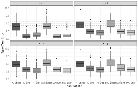
Figure 1: Type I error in $\%$ of the six versions of the QMANOVA divided into two types (ATS, MATS) and three covariance estimator (boot, int, ker). The results are divided by the sample size factor $K\in\{1,2,4,8\}$, i.e. $\mathbf{n}=K\mathbf{n}^{(r)}$, $r=1,2,3$.

To assess the tests’ performances for small and moderate sample sizes, we conducted a simulation study. The idea of the data generation is as follows. We generate median-centred data $\mathbf{e}_{ij}=\left(e_{ij1},\dots,e_{ijn_{i}}\right)^{\prime},\,e_{ij\ell}=Y_{ij\ell}-\text{median}(Y_{ij\ell})$ and choose for $Y_{ij\ell}$ the following five different distributions to cover symmetric and skewed scenarios: (a) the standard normal distribution $Y_{ij\ell}^{(1)}\sim N_{0,1}$, (b) the Student’s $t$-distribution with $2$ degrees of freedom $Y_{ij\ell}^{(2)}\sim t_{2}$, (c) the Student’s t-distribution with $3$ degrees of freedom $Y_{ij\ell}^{(3)}\sim t_{3}$, (d) the standard log-normal distribution $Y_{ij\ell}^{(4)}\sim LN_{0,1}$ and (e) the Chi-square distribution with $3$ degrees of freedom $Y_{ij\ell}^{(5)}\sim\chi^{2}_{3}$. Certain homoscedastic and hetereoscedastic covariance settings are realized by multiplying the square root of different covariance matrices to this data. Furthermore, we considered six different covariance matrices representing homoscedastic and heteroscedastic scenarios, which are displayed below for $d=4$:

1. $\mathbf{\Sigma}^{(1)}=\mathbf{I}_{d}-\frac{1}{2}\left(\mathbf{J}_{d}-\mathbf{I}_{d}\right)=\mathbf{\Sigma}^{(2)}$,

2. $\mathbf{\Sigma}^{(1)}=\left(0.6^{|a-b|}\right)_{a,b=1}^{d}=\mathbf{\Sigma}^{(2)}$,

3. $\mathbf{\Sigma}^{(1)}=\mathbf{I}_{d}+\frac{1}{2}\left(\mathbf{J}_{d}-\mathbf{I}_{d}\right),\,\mathbf{\Sigma}^{(2)}=3\,\mathbf{I}_{d}+\frac{1}{2}\left(\mathbf{J}_{d}-\mathbf{I}_{d}\right)$,

4. $\mathbf{\Sigma}^{(1)}=\left(0.6^{|a-b|}\right)_{a,b=1}^{d},\,\mathbf{\Sigma}^{(2)}=\left(0.6^{|a-b|}\right)_{a,b=1}^{d}+2\,\mathbf{I}_{d}$,

5. $\mathbf{\Sigma}^{(1)}=\begin{pmatrix}1&0.6&0.36&0.18\\ 0.6&1&0.6&0.3\\ 0.36&0.6&1&0.5\\ 0.18&0.3&0.5&0.25\end{pmatrix},\,\mathbf{\Sigma}^{(2)}=\mathbf{\Sigma}^{(1)}+0.5\,\mathbf{J}_{d}$,

6. $\mathbf{\Sigma}^{(1)}=\begin{pmatrix}1&0&0&0\\ 0&\sqrt{2}&0&0\\ 0&0&2&1\\ 0&0&1&0.5\end{pmatrix},\,\mathbf{\Sigma}^{(2)}=\mathbf{\Sigma}^{(1)}+0.5\,\mathbf{J}_{d}$.

Here, the fifth covariance setting is a modification form the second, where the elements $\sigma_{1dd}$, $\sigma_{1(d-1)d}$ and $\sigma_{1d(d-1)}$ of $\mathbf{\Sigma}^{(1)}$ are modified as described. The sixth setting is based on $\text{diag}(\sqrt{2^{s}})$ for $s\in\{0,\dots,d-1\}$, where the $d$-th row and column is replaced by half the row or rather the column before. To create data which is median centred, we calculate the empirical median $\mathbf{M}_{ij}$ of $(\mathbf{\Sigma}^{(i)})^{\frac{1}{2}}\mathbf{e}_{ij}$ from an extra sample with the size $n=10^{7}$ and withdraw $\mathbf{M}_{ij}$ from the data. Therefore, our simulated data can be described by the following model:

$$\mathbf{X}_{ij}=(\mathbf{\Sigma}^{(i)})^{\frac{1}{2}}\mathbf{e}_{ij}-\mathbf{M}_{ij}\sim F_{i},\,i\in\{1,\dots,k\},j\in\{1,\dots,n_{i}\}.$$

The aforementioned data generating process and the choice of the different settings is adapted from the one-way layout simulation in Friedrich and Pauly, (2018, Sec. 5). To consider small and large sample scenarios, we chose balanced and unbalanced small samples $\mathbf{n}^{(1)}=(10,10)^{\prime},\,\mathbf{n}^{(2)}=(10,20)^{\prime}$ and $\mathbf{n}^{(3)}=(20,10)^{\prime}$ as well as its multiples $K\cdot\mathbf{n}^{(r)}$ for $K\in\{2,4,8\}$. As a benchmark, we compare our method with the mean-based resampling MATS proposed by Friedrich and Pauly, (2018). This method is implemented in the R-package MANOVA.RM (Friedrich et al.,, 2022) as the functions MANOVA() or MANOVA.wide() (same tests for different data formats). We simulated two versions of the mean-based MATS, one is characterized by a parametric bootstrap and the other by a wild bootstrap with Rademacher weights, which are both implemented in the aforementioned package. All simulations are calculated with the computing environment R (R Core Team,, 2022), Version 4.0.0, for nsim = 5000 simulation runs and nboot = 2000 bootstrap iterations. As in Ditzhaus et al., (2021), we used the classical Gaussian kernel for the kernel density estimation and calculate the bandwidth $h$ by Silverman’s rule-of-thumb (Silverman,, 1998, Eq. 3.31) with the R-function bw.rnd0().

4.1 Type I Error

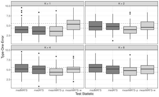
Figure 2: Type I error in $\%$ of the QMANOVA with bootstrap covariance estimator and the mean-based MATS by Friedrich and Pauly, (2018) with parametric (p) and wild (w) bootstrap for the one-way layout, the symmetric distributions ($N_{0,1}$, $t_{2}$, $t_{3}$), all covariance settings 1)- 6) as well as for balanced and unbalanced sample sizes $\mathbf{n}=K\cdot\mathbf{n}^{(r)}$ for $K\in\{1,2,4,8\}$.

In this subsection, we discuss the type I error control of all procedures in a one-way layout and present further results for a $2\times 2$-design in the supplement. In detail, we considered a multivariate set-up with $k=2$ groups and $d=\{4,8\}$ dimensions. Moreover, we restricted to the median $\mathbf{m}_{i},\,i\in\{1,2\}$, ($p=0.5$), because it is the most relevant quantile for statistical analysis and is comparable to the mean. This lead us to the null hypothesis $\mathcal{H}_{0}:\mathbf{m}_{1}=\mathbf{m}_{2}$ for the layout matrix $\mathbf{T}=\mathbf{P}_{2}\otimes\mathbf{I}_{4}$ and in all to $720$ different scenarios. In Figure 1, the different tests are named by a combination of the used test statistic and its covariance estimator. It is apparent that the bootstrap covariance estimator has the best performance regarding the type I error control. Overall, the MATS and the ATS test statistic have a similar type-one-error control. However, the MATS with the bootstrap covariance estimator performs the best as one can observe from the close position of the boxes to the binomial interval $[4.4,5.6]$. With the other covariance estimators, ATS and MATS show a quite conservative type I error control. In general, the observed type I error rates comes closer to the 5%-benchmark for larger $K$. This is in line with the theoretical findings from Section 3.1. All in all, we can only recommend the ATS and MATS combined with the bootstrap covariance estimator.

In the next step, we compare the two favorable QMANOVA methods, from now denoted by medMATS and medATS, with the mean-based MATS of Friedrich and Pauly, (2018) denoted by meanMATS-p and meanMATS-w to differentiate between the parametric (p) and wild (w) bootstrap versions. For a fair and appropriate comparison, we restrict ourselves to the symmetric distributions such that the mean-based hypothesis $\mathcal{H}_{0}:\boldsymbol{\mu}_{1}=\boldsymbol{\mu}_{2}$ and the median-based hypothesis $\mathcal{H}_{0}:\mathbf{m}_{1}=\mathbf{m}_{2}$ coincide. The type I error rates for all four tests are summarized in Table 1 for $\mathbf{n}^{(1)}=(10,10)$ and in the supplement for $\mathbf{n}^{(2)}$ and $\mathbf{n}^{(3)}$. For completeness reasons, we also include the error rates for two QMANOVA strategies for the nonsymmetric distributions $(LN_{0,1},\chi^{2}_{3}$). The results inside the binomial interval $[4.4,5.6]$ for the significance level $\alpha=5\%$ are printed in bold. A detailed study of Table 1 exhibits that the MATS performs slightly better than the ATS since the simulated type I errors are more frequent in $[4.4,5.6]$ for the MATS (17 times) than for the ATS (14 times). To further judge the performance for larger sample sizes, we summarized the type I error rates for all symmetric distributions and all different sample sizes $K\mathbf{n}^{(r)}$, $r=1,2,3$, in boxplots displayed in Figure 2 divided into the different choices of the scaling factor $K\in\{1,2,4,8\}$. In the Figure 2, the medMATS tends to be more conservative (empirical type I error smaller than $4.4$) and the meanMATS-w tends to be more liberal (empirical type I error larger than $5.6$). In case of small sample sizes $(K=1)$, the medATS and both MATS approaches exhibit a conservative type I error control for almost all settings. In settings with $d=8$ and the covariance choices 4) or 6), a conservative type I error control can even be found for larger samples $(K\in\{2,4,8\})$, see Table 1. Additionally, a liberal behaviour most often occurs for the covariance setting 5) in combination with the dimension $d=4$ (Table 1). For further details on the influence of the simulation scenarios’ aspects we refer to the Supplement. There, we explain that the choice of the covariance setting influences the performance most wile the QMANOVA method is mostly robust.Moreover, we also present type I error simulation study for a two-way layout in the supplement. There we simulated scenarios for a $2\times 2$ design with dimension $d=4$ for similar covariance settings. The corresponding findings are similar to the one-layout and thus omitted here.

$\Sigma$	Distr	$d=4$				$d=8$
		median		meanMATS		median		meanMATS
		MATS	ATS	param	wild	MATS	ATS	param	wild
1	$N_{0,1}$	2.4	2.0	3.2	4.0	2.4	2.8	3.2	4.0
	$t_{2}$	1.6	$\mathbf{4.4}$	2.0	4.0	4.0	6.0	4.0	6.8
	$t_{3}$	$\mathbf{4.8}$	$\mathbf{5.6}$	4.0	$\mathbf{4.4}$	$\mathbf{4.4}$	3.6	3.6	$\mathbf{4.4}$
	$LN_{0,1}$	3.2	3.6	-	-	$\mathbf{4.8}$	$\mathbf{4.4}$	-	-
	$\chi^{2}_{3}$	2.0	2.0	-	-	$\mathbf{4.8}$	4.0	-	-
2	$N_{0,1}$	$\mathbf{4.8}$	3.2	3.2	$\mathbf{4.4}$	$\mathbf{4.4}$	2.8	2.8	3.2
	$t_{2}$	$\mathbf{4.4}$	$\mathbf{4.4}$	$\mathbf{4.8}$	7.6	$\mathbf{4.8}$	$\mathbf{4.8}$	2.8	$\mathbf{5.2}$
	$t_{3}$	$\mathbf{4.4}$	3.6	3.6	$\mathbf{4.4}$	1.2	$\mathbf{4.4}$	3.6	$\mathbf{4.4}$
	$LN_{0,1}$	6.0	6.4	-	-	3.6	$\mathbf{5.2}$	-	-
	$\chi^{2}_{3}$	$\mathbf{5.2}$	$\mathbf{4.4}$	-	-	3.6	4.0	-	-
3	$N_{0,1}$	3.6	1.2	3.2	4.0	3.2	2.8	$\mathbf{4.8}$	7.2
	$t_{2}$	4.0	$\mathbf{4.8}$	3.2	6.4	3.6	3.2	3.2	$\mathbf{5.2}$
	$t_{3}$	2.8	2.8	3.6	$\mathbf{5.6}$	3.2	2.4	3.6	6.8
	$LN_{0,1}$	1.6	2.0	-	-	3.2	4.0	-	-
	$\chi^{2}_{3}$	6.0	3.6	-	-	4.0	2.4	-	-
4	$N_{0,1}$	1.6	1.6	2.4	3.6	2.8	2.8	$\mathbf{4.8}$	6.4
	$t_{2}$	4.0	2.4	2.4	$\mathbf{5.6}$	2.8	3.6	1.2	3.6
	$t_{3}$	3.6	3.2	1.2	1.6	2.8	2.0	2.8	$\mathbf{5.6}$
	$LN_{0,1}$	$\mathbf{4.8}$	$\mathbf{4.8}$	-	-	3.6	2.0	-	-
	$\chi^{2}_{3}$	$\mathbf{5.2}$	$\mathbf{5.6}$	-	-	2.4	1.6	-	-
5	$N_{0,1}$	8.8	8.4	8.8	9.6	$\mathbf{4.4}$	$\mathbf{4.8}$	$\mathbf{4.8}$	6.0
	$t_{2}$	3.6	3.6	$\mathbf{5.6}$	6.0	1.2	2.4	2.8	3.6
	$t_{3}$	7.6	8.4	6.0	6.0	4.0	3.2	$\mathbf{5.2}$	6.0
	$LN_{0,1}$	3.2	3.6	-	-	6.4	8.0	-	-
	$\chi^{2}_{3}$	8.4	6.4	-	-	$\mathbf{4.8}$	4.0	-	-
6	$N_{0,1}$	7.2	6.4	$\mathbf{4.8}$	$\mathbf{5.6}$	1.6	2.4	1.6	2.8
	$t_{2}$	$\mathbf{4.8}$	3.6	1.6	4.0	2.4	3.2	2.0	4.0
	$t_{3}$	4.0	$\mathbf{4.4}$	3.2	$\mathbf{4.4}$	2.8	$\mathbf{4.4}$	2.4	6.0
	$LN_{0,1}$	$\mathbf{5.6}$	6.8	-	-	3.2	2.8	-	-
	$\chi^{2}_{3}$	$\mathbf{5.2}$	3.2	-	-	4.0	6.4	-	-

Table 1: Type-I error rate in $\%$ (nominal level $\alpha=5\%$) for testing $\mathcal{H}_{0}:\mathbf{m}_{1}=\mathbf{m}_{2}$ in an one-way layout. We present all settings with the sample size $(10,\,10)$ of MATS and ATS combined with the bootstrap covariance estimator. The two comparing meanMATS models are named with meanMATS-p for a parametric bootstrap and with meanMATS-w for the wild bootstrap approach. The results inside the binomial interval for $\alpha$ $[4.4,5.6]$ are printed in bold.

4.2 Power

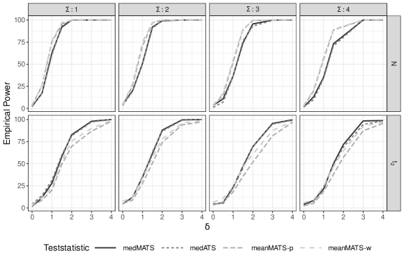
Figure 3: Empirical Power in Percent of the QMANOVA and the mean-based MATS by Friedrich and Pauly, (2018) for normal distributed (N) and $t_{2}$-distributed ($t_{2}$) data, the small sample size $(10,10)$ and the covariance settings $1-4$.

For the power comparison, we restrict to a representative subset of the settings from the previous section, namely to $d=4$, the covariance settings 1) - 4), the samples $Kn^{(1)}$ and $Kn^{(3)}$ for $K=2,4$ while we still consider all five distributions. To obtain alternative settings, we shift the data from the first group by $\delta\in\{0.5,1,1.5,2,3,4\}$, i.e. $\mathbf{X}_{1j}=\delta+\left((\mathbf{\Sigma}^{(1)})^{\frac{1}{2}}\mathbf{e}_{1j}-\mathbf{M}_{1j}\right),j\in\{1,\dots,n_{i}\}$ Moreover, we restrict to a representative subset of the settings, namely to $d=4$, the covariance settings 1) - 4), the samples $Kn^{(1)}$ and $Kn^{(3)}$ for $K=2,4$ while we still consider all five distributions. We again compare the two favorable QMANOVA methods with the mean-based MATS for symmetric distributions. Figure 3 includes the empirical power of the four methods for the normal and the $t_{2}$-distribution and all simulated covariance settings. Studying Figure 3 one can observe, that the mean-based tests are more powerful in the cases with the normal distribution, but for the $t_{2}$-distribution we can see the exact opposite. This observation fits to the power simulation results in Ditzhaus et al., (2021). There, an explanation for this is also given: mean and median are as location estimators asymptotically different efficient in the distributional scenarios. The sample median is the better location estimator in case of heavy-tailed data like the $t_{2}$-distribution, but for normal distributed data the situation is reversed. For all distributions the power increases faster for bigger sample sizes and again, the unbalanced designs do not seem to have any influence on this.

5 Illustrative Data Analysis

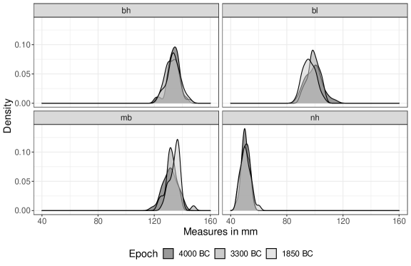
Figure 4: Kernel density estimates (Nadaraya,, 1965) based on Gaussian kernels of the four ($d=4$) characteristics of the skulls mb (maximal breadth), bh (basibregmatic height), bl (basialveolar length) and nh (nasal height) divided by three epochs ($k=3$) arround 4000 BC, around 3300 BC and around 1850 BC. The bandwidth of the kernel densities is chosen by Silverman’s rule-of-thumb (Silverman,, 1998, Eq. 3.31).

To illustrate the new methods on real data, we re-analyse the Egyptian skulls data set from Everitt and Hothorn, (2006) available in the R-Package HSAUR (Everitt and Hothorn,, 2022). For $90$ skulls, there are four variables ($d=4$) measured in mm and denoted by mb (maximal breadth), bh (basibregmatic height), bl (basialveolar length) and nh (nasal height). The skulls can be divided into three groups ($k=3$) which are characterised by time periods in years around 4000 BC ($i=1$), around 3300 BC ($i=2$) and around 1850 BC ($i=3$) (Oja,, 2010). The data is balanced with 30 skulls per group (Everitt and Hothorn,, 2022). All four measurements together characterize the skulls in their basic shape. We are interested in inferring whether there are differences between the three epochs. Figure 4 shows kernel density plots for each univariate measurement. We observe that the data is rather heavy-tailed and potentially heteroscedastic in each of the four measures. Thus, a median-based approach is reasonable leading to the multivariate null hypothesis $\mathcal{H}_{0}^{123}:\,\mathbf{m}_{1}=\mathbf{m}_{2}=\mathbf{m}_{3}$. Due to its convincing type I error control in our simulation study, we choose the quantile-based MATS combined with the bootstrap covariance estimator and compare it with the mean-based MATS (Friedrich and Pauly,, 2018) using wild bootstrap critical values. Similar to the simulation study, all tests are computed based upon $2,000$ bootstrap iterations. The resulting $p$-values are given in Table 2.

Test	Hypothesis
	$\mathcal{H}_{0}^{123}:$	$\mathcal{H}_{0}^{12}:$	$\mathcal{H}_{0}^{23}:$	$\mathcal{H}_{0}^{13}:$
	$\mathbf{m}_{1}=\mathbf{m}_{2}=\mathbf{m}_{3}$	$\mathbf{m}_{1}=\mathbf{m}_{2}$	$\mathbf{m}_{2}=\mathbf{m}_{3}$	$\mathbf{m}_{1}=\mathbf{m}_{3}$
medMATS	$0.038^{*}$	$0.726$	$0.042^{*}$	$0.007^{*}$
meanMATS-w	$0.062$	$0.756$	$0.061$	$0.038$

Table 2: $p$-values for the different null hypotheses and the tests medMATS (quantile-based MATS with bootstrap covariance estimator) and meanMATS-w (mean-based MATS with wild bootstrap resampling). The $p$-values marked with a ^∗ indicate the rejected hypootheses at multiple level $5\%$.

It can be seen, that the medMATS rejects the null hypothesis at significance level $0.05$ whereas the mean-based meanMATS-w does not. A probable reason for this is that the data is nearly symmetric and heavy-tailed in all dimensions (cf. Figure 4). In such settings the medMATS exhibit a better power performance compared to meanMATS-w. After rejecting this global null hypothesis, it is intuitive to perform group-wise post hoc analyses. Consequently, one can formulate all pairs hypotheses: $\mathcal{H}_{0}^{12}:\mathbf{m}_{1}=\mathbf{m}_{2}$, $\mathcal{H}_{0}^{23}:\mathbf{m}_{2}=\mathbf{m}_{3}$ and $\mathcal{H}_{0}^{13}:\mathbf{m}_{1}=\mathbf{m}_{3}$. The tests’ p-values are displayed in Table 2. Altogether, the considered hypotheses form a closed testing procedure (Gabriel,, 1969) and thus do not need adjustment. That is why the multiple meanMATS-w and medMATS tests control the family-wise-error-rate without an extra adjustment of the $p$-values. We obtain different test results from both methods: The multiple medMATS test rejects the global null and detects a difference in the 3300 BC and the 1850 BC skulls at the 5% level. In comparison, the multiple mean-based meanMATS-w test does not reject the global null hypothesis $\mathcal{H}_{0}^{123}$ at the 5% level. Thus, it would also not detect the difference between the 3300 BC and the 1850 BC skulls as no pairwise posthoc comparisons would have been performed.

6 Conclusion and Outlook

We have introduced six statistical tests in a general MANOVA-set-up (QMANOVA) regarding marginal quantiles . These are based on different test statistics: an ANOVA-type statistic (ATS) and a modified ATS (MATS), both in combination with three different covariance estimators (based on a kernel, bootstrap and interval-based approach). All statistics are quadratic forms in the normalized vector of pooled quantiles and can be seen as a generalization of the univariate QANOVA presented in Ditzhaus et al., (2021). As all test statistics are no asymptotic pivots, we propose a non-parametric bootstrap approach to calculate critical values. We analyze the corresponding limit behavior and prove that the resulting tests are asymptotic exact and consistent.In fact, the methods are asymptotically valid in general factorial designs and do not postulate homoscedasticity or a specific distribution. In an extensive simulation study focusing on the median, it turned out that the MATS with the bootstrap covariance estimator performs the best among the six proposed QMANOVA methods. In particular, it is robust against various aspects of data and performs well on heavy-tailed and skewed data with equal, unequal and singular covariance structures. We additionally compared its performance with the mean-based MATS proposed by Friedrich and Pauly, (2018) as benchmark method. In-line with theoretical properties of means and medians, our power simulation study showed that the median-based QMANOVA performs better than the corresponding mean-based approach in terms of power. This has also been confirmed in an illustrative data analyses with symmetric and heavy-tailed data in a three-way MANOVA setting. The test results suggest that using the QMANOVA instead of an mean-based method is an added value in this application.

Apart from the illustrative data analyses, the focus of the paper was on deriving global test procedures. Having rejected a global null, post-hoc analyses on the components or factor levels are of interest and multiplicity may become an issue. In the three-way MANOVA setting of the data example this was no issue. But it would be for more complex situtations. Thus, we plan to derive multiple contrast tests (MCTs) for contrasts of marginal medians and quantiles in the future. Here, concepts from Gunawardana and Konietschke, (2019) could be adapted. As the derived methods can directly be inverted in confidence regions we would also like to derive simultaneous confidence regions and intervals that are compatible to the MCTs decisions. This would allow a deeper insight into the behaviour of the estimates. Moreover, similar to mean-based MANCOVA (Zimmermann et al.,, 2020), we plan to derive QMANCOVAs that allow for covariate adjustments.

7 Acknowledgement

This work has been partly supported by the Research Center Trustworthy Data Science and Security (https://rc-trust.ai), one of the Research Alliance centers within the UA Ruhr.

Appendix A Additional Simulation Results

A.1 Additional Results regarding the One-Way Layout

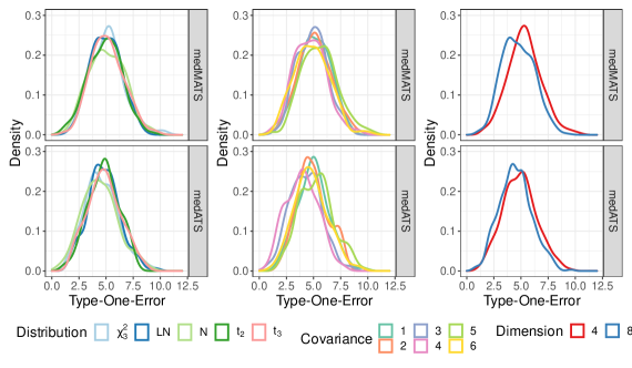
Figure 5: Kernel density estimators (Nadaraya,, 1965) based on Gaussian kernels of all simulation results for the type I error of the one-way layout divided by the distribution, the covariance and the dimension of the simulation scenarios. The bandwidth of the kernel densities is chosen by Silverman’s rule-of-thumb (Silverman,, 1998, Eq. 3.31).

$\Sigma$	Distr	$d=4$				$d=8$
		median		meanMATS		median		meanMATS
		MATS	ATS	param	wild	MATS	ATS	param	wild
1	$N_{0,1}$	6.8	6.0	$\mathbf{5.6}$	6.0	3.6	$\mathbf{4.4}$	$\mathbf{4.8}$	6.8
	$t_{2}$	4.0	3.2	2.8	$\mathbf{4.8}$	2.8	3.2	6.0	6.4
	$t_{3}$	4.0	4.0	$\mathbf{4.8}$	6.0	2.4	2.4	$\mathbf{4.4}$	$\mathbf{5.2}$
	$LN_{0,1}$	$\mathbf{4.4}$	3.6	-	-	$\mathbf{5.2}$	$\mathbf{5.2}$	-	-
	$\chi^{2}_{3}$	6.8	$\mathbf{5.2}$	-	-	3.2	$\mathbf{5.2}$	-	-
2	$N_{0,1}$	6.4	$\mathbf{5.2}$	6.4	6.8	$\mathbf{4.8}$	$\mathbf{4.4}$	6.4	7.2
	$t_{2}$	$\mathbf{5.2}$	$\mathbf{5.2}$	$\mathbf{4.4}$	6.8	4.0	3.6	4.0	6.8
	$t_{3}$	8.4	7.6	$\mathbf{5.2}$	7.2	4.0	6.4	3.2	$\mathbf{4.4}$
	$LN_{0,1}$	$\mathbf{4.8}$	$\mathbf{5.2}$	-	-	$\mathbf{5.6}$	4.0	-	-
	$\chi^{2}_{3}$	4.0	3.2	-	-	2.8	3.2	-	-
3	$N_{0,1}$	6.0	6.8	$\mathbf{5.6}$	6.8	3.2	3.6	$\mathbf{4.4}$	$\mathbf{5.6}$
	$t_{2}$	$\mathbf{4.8}$	4.0	2.8	$\mathbf{5.2}$	$\mathbf{4.8}$	$\mathbf{5.2}$	4.0	$\mathbf{5.6}$
	$t_{3}$	$\mathbf{5.6}$	$\mathbf{5.2}$	$\mathbf{5.6}$	6.0	3.6	$\mathbf{5.2}$	$\mathbf{4.4}$	6.0
	$LN_{0,1}$	3.2	2.8	-	-	$\mathbf{5.6}$	6.4	-	-
	$\chi^{2}_{3}$	$\mathbf{4.8}$	$\mathbf{4.4}$	-	-	$\mathbf{4.4}$	$\mathbf{5.2}$	-	-
4	$N_{0,1}$	$\mathbf{4.4}$	2.8	$\mathbf{4.4}$	$\mathbf{4.4}$	3.6	0.8	2.4	3.6
	$t_{2}$	2.8	3.6	2.4	2.4	3.2	3.2	1.2	6.0
	$t_{3}$	3.6	3.6	3.6	4.0	$\mathbf{5.6}$	4.0	2.4	6.0
	$LN_{0,1}$	6.4	$\mathbf{5.2}$	-	-	2.8	2.8	-	-
	$\chi^{2}_{3}$	$\mathbf{4.8}$	4.0	-	-	3.6	4.0	-	-
5	$N_{0,1}$	$\mathbf{4.8}$	$\mathbf{5.2}$	$\mathbf{5.2}$	6.0	2.8	2.0	2.8	4.0
	$t_{2}$	$\mathbf{4.8}$	$\mathbf{4.4}$	3.6	$\mathbf{4.4}$	2.8	2.4	3.2	$\mathbf{5.6}$
	$t_{3}$	$\mathbf{5.6}$	6.4	8.0	8.8	$\mathbf{5.2}$	3.6	3.2	$\mathbf{4.8}$
	$LN_{0,1}$	3.6	4.0	-	-	4.0	3.6	-	-
	$\chi^{2}_{3}$	$\mathbf{5.6}$	6.0	-	-	$\mathbf{5.2}$	4.0	-	-
6	$N_{0,1}$	$\mathbf{4.8}$	7.2	6.0	7.2	2.8	2.0	2.4	3.6
	$t_{2}$	4.0	$\mathbf{4.8}$	2.4	$\mathbf{4.8}$	2.4	3.2	0.8	3.6
	$t_{3}$	4.0	$\mathbf{4.4}$	3.2	4.0	4.0	6.0	2.0	2.4
	$LN_{0,1}$	$\mathbf{4.4}$	2.8	-	-	2.4	$\mathbf{4.4}$	-	-
	$\chi^{2}_{3}$	$\mathbf{4.8}$	4.0	-	-	$\mathbf{4.4}$	3.2	-	-

Table 3: Type I error rate in $\%$ (nominal level $\alpha=5\%$) for testing $\mathcal{H}_{0}:\mathbf{m}_{1}=\mathbf{m}_{2}$ in an one-way layout. We present all settings with the sample size $(10,\,20)$ of MATS and ATS combined with the bootstrap covariance estimator. The two comparing meanMATS models are named with meanMATS-p for a parametric bootstrap and with meanMATS-w for the wild bootstrap approach. The results inside the binomial interval for $\alpha$ $[4.4,5.6]$ are printed in bold.

$\Sigma$	Distr	$d=4$				$d=8$
		median		meanMATS		median		meanMATS
		MATS	ATS	param	wild	MATS	ATS	param	wild
1	$N_{0,1}$	$\mathbf{4.8}$	$\mathbf{4.4}$	6.0	$\mathbf{5.6}$	$\mathbf{4.8}$	$\mathbf{4.8}$	$\mathbf{5.2}$	6.0
	$t_{2}$	3.6	3.2	$\mathbf{5.2}$	6.4	4.0	4.0	3.2	4.0
	$t_{3}$	6.4	$\mathbf{4.8}$	6.0	6.4	$\mathbf{4.4}$	$\mathbf{4.8}$	3.2	3.6
	$LN_{0,1}$	4.0	3.6	-	-	$\mathbf{4.8}$	6.8	-	-
	$\chi^{2}_{3}$	$\mathbf{5.2}$	3.2	-	-	$\mathbf{4.4}$	$\mathbf{4.8}$	-	-
2	$N_{0,1}$	3.2	3.6	$\mathbf{4.4}$	$\mathbf{4.8}$	3.2	2.8	$\mathbf{4.4}$	$\mathbf{4.8}$
	$t_{2}$	3.2	2.4	4.0	$\mathbf{5.6}$	2.0	2.4	1.6	$\mathbf{4.8}$
	$t_{3}$	4.0	$\mathbf{5.2}$	2.4	2.8	2.4	2.0	3.2	4.0
	$LN_{0,1}$	$\mathbf{5.2}$	$\mathbf{5.6}$	-	-	4.0	$\mathbf{4.4}$	-	-
	$\chi^{2}_{3}$	7.6	7.2	-	-	4.0	3.2	-	-
3	$N_{0,1}$	2.8	2.0	2.8	2.8	$\mathbf{4.8}$	3.2	3.6	6.4
	$t_{2}$	$\mathbf{5.6}$	6.4	3.6	6.8	3.2	2.0	1.6	2.4
	$t_{3}$	$\mathbf{5.2}$	$\mathbf{4.4}$	$\mathbf{4.4}$	$\mathbf{5.6}$	3.2	3.2	1.6	4.0
	$LN_{0,1}$	4.0	2.4	-	-	3.6	3.2	-	-
	$\chi^{2}_{3}$	6.0	6.8	-	-	3.2	3.6	-	-
4	$N_{0,1}$	3.6	2.4	$\mathbf{4.8}$	$\mathbf{5.6}$	3.6	1.6	4.0	$\mathbf{5.6}$
	$t_{2}$	1.6	1.6	2.0	2.8	1.2	1.2	1.6	4.0
	$t_{3}$	$\mathbf{5.6}$	2.4	1.6	1.6	$\mathbf{4.4}$	2.0	2.0	$\mathbf{5.6}$
	$LN_{0,1}$	$\mathbf{4.4}$	2.0	-	-	2.8	2.0	-	-
	$\chi^{2}_{3}$	$\mathbf{4.8}$	4.0	-	-	$\mathbf{5.2}$	3.2	-	-
5	$N_{0,1}$	8.8	8.4	7.6	8.4	$\mathbf{4.8}$	3.6	4.0	$\mathbf{4.8}$
	$t_{2}$	4.0	2.8	3.2	4.0	6.8	$\mathbf{5.2}$	4.0	$\mathbf{4.4}$
	$t_{3}$	9.6	8.4	6.8	7.6	$\mathbf{4.8}$	$\mathbf{4.4}$	6.4	7.2
	$LN_{0,1}$	6.0	$\mathbf{5.2}$	-	-	$\mathbf{5.2}$	6.0	-	-
	$\chi^{2}_{3}$	6.8	6.8	-	-	$\mathbf{5.6}$	6.4	-	-
6	$N_{0,1}$	$\mathbf{5.6}$	6.0	$\mathbf{5.6}$	6.4	2.4	2.8	2.0	3.2
	$t_{2}$	6.4	4.0	3.2	6.8	3.2	4.0	1.6	3.2
	$t_{3}$	6.4	7.2	4.0	6.8	4.0	$\mathbf{4.4}$	2.4	6.8
	$LN_{0,1}$	4.0	$\mathbf{4.8}$	-	-	2.0	3.6	-	-
	$\chi^{2}_{3}$	2.4	2.0	-	-	3.6	2.4	-	-

Table 4: Type I error rate in $\%$ (nominal level $\alpha=5\%$) for testing $\mathcal{H}_{0}:\mathbf{m}_{1}=\mathbf{m}_{2}$ in an one-way layout. We present all settings with the sample size $(20,\,10)$ of MATS and ATS combined with the bootstrap covariance estimator. The two comparing meanMATS models are named with meanMATS-p for a parametric bootstrap and with meanMATS-w for the wild bootstrap approach. The results inside the binomial interval for $\alpha$ $[4.4,5.6]$ are printed in bold.

To get a deeper insight into the tests performance, we present the result of the type I error simulation study as density plots divided by certain aspects. The left column in Figure 5 presents the density divided by the different distributions, the middle column by the covariance settings and the right column by the dimension. Thus, it becomes clear which aspects influence the tests performance. The right column shows that the different dimensions have almost none influence on the tests’ performance in both methods. On the contrary, there are clear differences between the covariance settings. They seem to have the most influence on the type I errors in this comparison. Here, the type I errors for the ATS statistic with bootstrap covariance estimator differs more than the errors for the MATS statistic. This phenomenon can also be observed in the first column of Figure 5; and even for the standard normal distribution, the ATS statistic produces in average too small type I errors. This can also be observed in Figure 1 and 2 of the paper. All simulation results of the type I error for the sample sizes $(10,\;20)$ and $(20,\;10)$ are presented in in Tables 3 and 4. There, it can be seen, that the unbalanced sample size seems to have no influence of the tests performance. Tendentiously, the behaviour gets better as the sample size gets larger. All in all, Figure 5 shows that the QMANOVA method is still robust against various distributional scenarios. This is consistent with our theoretical results.

A.2 Two-way-Layout

To get more insights into our method, we analyse the behaviour in the case of a two-way-layout in the following set-up. We consider two crossed factors $A$ and $B$ having two levels each with the sample sizes $n^{(4)}=(n_{ab})_{a,b=1,2}=(n_{11},n_{12},n_{21},n_{22})=(7,10,13,16),$ $\;n^{(5)}=(10,10,10,10)$, $n^{(6)}=(16,13,10,7),$ $n^{(7)}=(20,20,20,20),$ $n^{(8)}=(100,100,100,100)$, $n^{(9)}=(100,50,100,50)$, $n^{(10)}=(15,15,$ $15,15)$, $n^{(11)}=(14,20,$ $16,32)$ and $n^{(12)}=(32,26,20,14)$. The data generating process and the distributions are identical to the simulation study for a one-way layout and use the following covariance settings with $d=4$ dimensions:

1. $\mathbf{\Sigma}^{(i_{1}i_{2})}=\mathbf{I}_{d}-\frac{1}{2}\left(\mathbf{J}_{d}-\mathbf{I}_{d}\right),\;i_{1},i_{2}\in\{1,2\}$,

2. $\mathbf{\Sigma}^{(i_{1}i_{2})}=\left(0.6^{|a-b|}\right)_{a,b=1}^{d},\;i_{1},i_{2}\in\{1,2\}$,

3. $\mathbf{\Sigma}^{(i_{1}i_{2})}=\xi\,\mathbf{I}_{d}+\frac{1}{2}\left(\mathbf{J}_{d}-\mathbf{I}_{d}\right),\;\xi\in\{1,\dots,4\}$,

4. $\mathbf{\Sigma}^{(i_{1}i_{2})}=\left(0.6^{|a-b|}\right)_{a,b=1}^{d}+\xi\,\mathbf{I}_{d},\;\xi\in\{1,\dots,4\}.$

We consider three different hypotheses to the significance level $\alpha=0.05$:

• The hypothesis of no effect of factor $A$

  $$\mathcal{H}_{0}(A):\left(\mathbf{P}_{2}\otimes\frac{1}{2}\mathbf{J}_{2}\otimes\mathbf{I}_{4}\right)\mathbf{q}=\mathbf{0}_{8}\Leftrightarrow\mathcal{H}_{0}(A):\mathbf{\bar{q}}_{1\cdot}=\mathbf{\bar{q}}_{2\cdot},$$

• the hypothesis of no effect of factor $B$

  $$\mathcal{H}_{0}(B):\left(\frac{1}{2}\mathbf{J}_{2}\otimes\mathbf{P}_{b}\otimes\mathbf{I}_{4}\right)\mathbf{q}=\mathbf{0}_{8}\Leftrightarrow\mathcal{H}_{0}(B):\mathbf{\bar{q}}_{\cdot 1}=\mathbf{\bar{q}}_{\cdot 2},$$

• the hypothesis of no $A\times B$ interaction effect

  $$\mathcal{H}_{0}(AB):\left(\mathbf{P}_{2}\otimes\mathbf{P}_{2}\otimes\mathbf{I}_{4}\right)\mathbf{q}=\mathbf{0}_{8}.$$

This leads to $540$ different scenarios and the whole set-up is similar to the simulations in Friedrich and Pauly, (2018); the mean-based MATS is our comparing method again. In general, QMANOVA’s performance for the two-way layout is similar to the performance in the one-way-layout. Again, the bootstrap covariance estimator performs best and the performance of the two test statistics is similar. In the upper graph of Figure 6 this result is shown for the symmetric distributions. The performance of medMATS is similar to the meanMATS-w and analogously to the simulations regarding the one-way layout, the medMATS tends to be conservative and the meanMATS-w tends to be more liberal. With the density plots in the lower graph of Figure 6, we analyse again the influence of the distribution, the covariance and the test layout on the test’s performance. In the distribution and the covariance column, one can see more variation than in the equivalent figures of the one-way layout. Since the layout is more complex, this observation is not surprising and leads us to the question if the two-way layout works with the very small sample size of $(10,\,10)$ as the one-way layout does. In the situation of such small samples, the QMANOVA methods tend to be conservative. Figure 8 compares the tests performance regarding the sample size. Here, the largest sample sizes $n^{(8)}=(100,100,100,100)$ and $n^{(9)}=(100,50,100,50)$ are excluded from the analyses. It is apparent from this figure, that the tests performance is very well for the sample sizes $n^{(7)}=(20,20,20,20),\;n^{(11)}=(14,20,16,32)$ and $n^{(12)}=(32,26,20,14)$. The smaller samples seems to be too small for the QMANOVA, because the simulations study produces there fairly too conservative type I errors. For the two-way layout, most empirical type I errors under $4.4$, the lower bound of the $95\%$ binomial interval, are from small sample sizes. Furthermore, it can be observed, that the QMANOVA can handle unbalanced scenarios equally well as the balanced ones. As in the settings regarding a one-way layout, the medMATS with the bootstrap covariance estimator is the best QMANOVA method. Here, the settings with conservative behaviour (empirical type I error smaller than $4.4$) have often covariance settings $9$ or $10$, if they have not small sample sizes. Again, conservative values appear more frequently than liberal one (empirical type I error bigger than $5.6$). Looking at all results with liberal behaviour, there is the reversed situation as for the conservative results: the settings with liberal behaviour have often covariance settings $7$ and $8$. From this it follows that unequal covariances seem to be a problem in a two-way layout, this was not observable in the one-way layout. In summary, the unequal covariances have a clear effect on the simulation results in the two-way layout, which was not the case in the one-way layout.

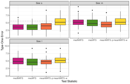
Figure 6: Type I error (in percent) for the symmetric distributions ($N_{0,1}$, $t_{2}$, $t_{3}$) in the two-way-layout simulations study for the QMANOVA with bootstrap covariance estimator and the mean-based MATS by Friedrich and Pauly, (2018) with parametric (p) and wild (w) bootstrap as resampling technique. The results are divided by sample size. Here, the samples $n^{(4)},\,n^{(5)}$ and $n^{(6)}$ are categorized as small (s), the samples $n^{(7)}$ and $n^{(10)}-n^{(12)}$ as middle (m) and the samples $n^{(8)}$ and $n^{(9)}$ as large (l).

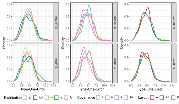
Figure 7: Kernel density estimators (Nadaraya,, 1965) based on Gaussian kernels of all simulation results for the type I error of the two-way layout divided by the distribution, the covariance and the layouts of the simulation scenarios. The bandwidth of the kernel densities is chosen by Silverman’s rule-of-thumb (Silverman,, 1998, Eq. 3.31).

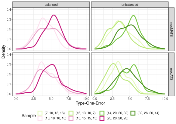
Figure 8: Kernel density estimators (Nadaraya,, 1965) based on Gaussian kernels of all simulation results for the type I error of the two-way layout divided by the sample sizes. The bandwidth of the kernel densities is chosen by Silverman’s rule-of-thumb (Silverman,, 1998, Eq. 3.31).

Appendix B Mathematical Foundation of the Proposition 6

The vector of group-specific marginal empirical distribution functions is equal to

$$\begin{pmatrix}\hat{F}_{i1}(t_{1})\\ \vdots\\ \hat{F}_{id}(t_{d})\end{pmatrix}=\frac{1}{n_{i}}\sum_{j=1}^{n_{i}}\begin{pmatrix}\mathbf{1}_{(-\infty,t_{1}]}(X_{ij1})\\ \vdots\\ \mathbf{1}_{(-\infty,t_{d}]}(X_{ijd})\end{pmatrix}=\frac{1}{n_{i}}\sum_{j=1}^{n_{i}}\begin{pmatrix}\mathbf{1}_{(-\infty,t_{1}]\times\mathbb{R}^{d-1}}(X_{ij1},\dots,X_{ijd})\\ \vdots\\ \mathbf{1}_{\mathbb{R}^{d-1}\times(-\infty,t_{d}]}(X_{ij1},\dots,X_{ijd})\end{pmatrix}.$$ (11)

For $t\in\mathbb{R}$ and $\ell,r\in\{1,\dots,d\}$, set $A_{t\ell r}=(-\infty,t]$ if $\ell=r$ and $A_{t\ell r}=\mathbb{R}$ else. Then, the functions

$$f_{t\ell}:=\mathbf{1}_{\bigotimes_{r=1}^{d}A_{t\ell r}}:\mathbb{R}^{d}\to\mathbb{R},\,\begin{pmatrix}x_{1}\\ \vdots\\ x_{d}\end{pmatrix}\mapsto f_{t\ell}(x_{1},\dots,x_{d}) =\mathbf{1}_{\bigotimes_{r=1}^{d}A_{t\ell r}}(x_{1},\dots,x_{d})$$

$$=\begin{cases}1,\;x_{\ell}\in A_{t\ell\ell}=(-\infty,t]\\ 0,\;x_{\ell}\not\in A_{t\ell\ell}=(-\infty,t]\end{cases}$$

characterize the marginal empirical distribution functions and they form a set:

$$\mathcal{E}:=\left\{f_{t\ell}=\mathbf{1}_{\bigotimes_{r=1}^{d}A_{t\ell r}}|A_{t\ell\ell}=(-\infty,t]\land A_{t\ell r}=\mathbb{R}:r\not=\ell;\,r,\ell\in\{1,\dots,d\}\land t\in\mathbb{R}\right\}.$$

Lemma 10.

The set of measurable functions $\mathcal{E}$ is a VC-class.

Proof.

Due to Problem 9 in Section 2.6 of van der Vaart and Wellner, (2000, p. 151) it remains to show that

$$\mathcal{C}=\left\{\bigotimes_{r=1}^{d}A_{t\ell r}|A_{t\ell\ell}=(-\infty,t]\land A_{t\ell r}=\mathbb{R}:\,r\neq\ell\in\{1,\ldots,d\}\land t\in\mathbb{R}\right\}$$

is a VC-class. We use the fact that the $d$-dimensional cells

$$\mathcal{D}=\left\{\bigotimes_{r=1}^{d}A_{r}|A_{r}=(-\infty,t_{r}]:r\in\{1,\ldots,d\}\land t_{r}\in\mathbb{R}\right\}$$

form a VC-class with VC-index $d+1$ (cf. van der Vaart and Wellner,, 2000, Ex. 2.6.1). To prove that $\mathcal{C}$ is a VC-class, let us suppose for a moment that $\mathcal{C}$ shatters the subset $\{\mathbf{x}_{1},\ldots,\mathbf{x}_{m}\}\subset\mathbb{R}^{d}$ for some $m\in\mathbb{N}$, e.g. every subset $\mathbf{X}$ of $\{\mathbf{x}_{1},\ldots,\mathbf{x}_{m}\}$ can be written as an intersection between $\{\mathbf{x}_{1},\ldots,\mathbf{x}_{m}\}$ and an element $C\in\mathcal{C}$: $\mathbf{X}=\{\mathbf{x}_{1},\ldots,\mathbf{x}_{m}\}\cap C$. Define $M=\max\left\{x_{sr}|s\in\{1,\ldots,m\};r\in\{1,\dots,d\}\right\}+1$. Thus, $M$ is larger than any component of $\mathbf{x}_{1},\ldots,\mathbf{x}_{m}$. Then it is clear that

$$\mathcal{C}^{\prime}=\left\{\bigotimes_{r=1}^{d}A_{t\ell r}|A_{t\ell\ell}=(-\infty,t]\land A_{tr\ell}=(-\infty,M]:r\neq\ell\in\{1,\ldots,d\}\land t\in\mathbb{R}\right\}$$

shatters $\{\mathbf{x}_{1},\ldots,\mathbf{x}_{m}\}\subset\mathbb{R}^{d}$ as well. Since $\mathcal{C}^{\prime}$ is clearly a subset of $\mathcal{D}$, $\mathcal{C}^{\prime}$ is for $m\leq d+1$ also a VC-class with VC-index $d+1$ or smaller. This is a contradiction. Thus, $\mathcal{C}$ does not shatter the subset $\{\mathbf{x}_{1},\ldots,\mathbf{x}_{m}\}\subset\mathbb{R}^{d}$ and it can finally be deduced that $\mathcal{C}$ is a VC-class with a VC-index smaller or equal to $d+1$. ∎

The set $\mathcal{E}$ corresponds to the marginal empirical distribution functions because the empirical measure of the functions in $\mathcal{E}$ create them, compare Formula (11). Categorizes the set $\mathcal{E}$ as a VC-Class amounts to apply the theory of empirical processes on the marginal empirical distribution functions. Applying Theorem 2.6.7 in van der Vaart and Wellner, (2000), Lemma 10 yields that $\mathcal{E}$ satisfies the uniform entropy condition (2.5.1) in van der Vaart and Wellner, (2000, p. 127). The function

$$\mathbf{1}_{\mathbb{R}^{d}}:\mathbb{R}^{d}\to\mathbb{R},\;(x_{1},\dots,x_{d})\mapsto 1$$

is an envelope function for $\mathcal{E}$ and it holds for every distribution $P$ on $\left(\mathbb{R}^{d},\mathcal{B}\left(\mathbb{R}^{d}\right)\right)$

$$\left(\int|\mathbf{1}_{\mathbb{R}^{d}}|^{2}dP\right)^{\frac{1}{2}}=\left(\int_{\mathbb{R}^{d}}\mathbf{1}dP\right)^{\frac{1}{2}}=(P(\mathbb{R}^{d}))^{\frac{1}{2}}=1<\infty.$$

From these three conditions it can be concluded that $\mathcal{E}$ is $P$-Donsker (cf. van der Vaart and Wellner,, 2000, p. 141). Consequently:

$$\sqrt{n_{i}}\left(\hat{F}_{i\ell}-F_{i\ell}\right)_{\ell\in\{1,\dots,d\}}\stackrel{{\scriptstyle d}}{{\longrightarrow}}\mathbb{G}_{i}\;\text{in}\;\ell^{\infty}(\mathcal{E}),\;i\in\{1,\dots,k\}.$$

By construction the limit process $\mathbb{G}_{i}:\mathcal{E}\to\mathbb{R},\,f\mapsto\mathbb{G}_{i}f$ is a empirical process in $\ell^{\infty}(\mathcal{E})$ for every $i\in\{1,\dots,k\}$. It can also be written as $\{\mathbb{G}_{i}f_{t\ell}|f_{t\ell}\in\mathcal{E}\}$ and is furthermore a zero-mean Gaussian process (cf. van der Vaart and Wellner,, 2000, p. 81 f.). Its covariance is constructed as follows: Let $f_{t\ell}=\mathbf{1}_{\bigotimes_{r=1}^{d}A_{t\ell r}},\,f_{sm}=\mathbf{1}_{\bigotimes_{r=1}^{d}B_{smr}}\in\mathcal{E}$. Thus, it holds $A_{t\ell\ell}=(-\infty,t],\,B_{smm}=(-\infty,s]$ and $A_{t\ell r}=B_{smr}=\mathbb{R}$ for the other $r\in\{1,\dots,d\}$ and (cf. van der Vaart and Wellner,, 2000, Equation (2.1.2))

$$\text{Cov}(\mathbb{G}_{i}f_{t\ell},\mathbb{G}_{i}f_{sm}) =E\mathbb{G}_{i}f_{t\ell}\mathbb{G}_{i}f_{sm}=P_{i}f_{t\ell}f_{sm}-P_{i}f_{t\ell}P_{i}f_{sm}$$

$$=P_{i}\left(\bigotimes_{r=1}^{d}A_{t\ell r}\cap\bigotimes_{r=1}^{d}B_{smr}\right)-P_{i}\left(\bigotimes_{r=1}^{d}A_{t\ell r}\right)P_{i}\left(\bigotimes_{r=1}^{d}B_{smr}\right)$$

$$=P_{i}\left(\bigotimes_{r=1}^{d}\left(A_{t\ell r}\cap B_{smr}\right)\right)-P_{i}\left(\bigotimes_{r=1}^{d}A_{t\ell r}\right)P_{i}\left(\bigotimes_{r=1}^{d}B_{smr}\right).$$

For $\ell=m$ it follows that $A_{t\ell\ell}=(-\infty,t]$ and $B_{smm}=(-\infty,s]$ and thus $A_{t\ell\ell}\cap B_{smm}=(-\infty,\min(t,s)]$. And for $\ell\not=m$ follows that $A_{t\ell\ell}=(-\infty,t],\,B_{sm\ell}=\mathbb{R},\,A_{t\ell m}=\mathbb{R}$ and $B_{smm}=(-\infty,s]$ and thus $A_{t\ell\ell}\cap B_{sm\ell}=(-\infty,t]$ and $A_{t\ell m}\cap B_{smm}=(-\infty,s]$. For the covariance this means:

$$\text{Cov}(\mathbb{G}_{i}f_{t\ell},\mathbb{G}_{i}f_{sm})=\begin{cases}F_{i\ell}\left(\min(t,s)\right)-F_{i\ell}(s)F_{i\ell}(t),\;\ell=m\\ F_{im\ell}(s,t)-F_{i\ell}(t)F_{im}(s),\;\ell\not=m\end{cases}.$$

By Lemma 1.5.3 in van der Vaart and Wellner, (2000) this characterizes $\mathbb{G}_{i}$ in $\ell^{\infty}(\mathcal{E})$ completely. For a fixed $\ell\in\{1,\dots,d\}$ any function $f_{t\ell}\in\mathcal{E}$ can be identified with $t\in\mathbb{R}$, and thus, $\ell^{\infty}(\mathcal{E})$ with $\left[\ell^{\infty}\left(\mathbb{R}\right)\right]^{d}$ (cf. van der Vaart and Wellner,, 2000, Example 2.1.3). The Skorokhod Space $D(\mathbb{R})$ contains all right-continuous functions $G:\mathbb{R}\to\mathbb{R}$ with left limits (cf. van der Vaart and Wellner,, 2000, p. 3). When the space is equipped with the supremum norm $\|G\|=\sup_{t\in\mathbb{R}}|G(t)|$, the weak convergence in $D(\mathbb{R})^{d}$ follows from the weak convergence in $\left[\ell^{\infty}\left(\mathbb{R}\right)\right]^{d}$ (cf. van der Vaart and Wellner,, 2000, Example 2.1.3). Thus, the convergence in distribution holds also in $D(\mathbb{R})^{d}$:

$$\sqrt{n_{i}}\left(\hat{F}_{i\ell}-F_{i\ell}\right)_{\ell\in\{1,\dots,d\}}\stackrel{{\scriptstyle d}}{{\longrightarrow}}\mathbb{G}_{i}\;\text{in}\;D(\mathbb{R})^{d},\;i\in\{1,\dots,k\}.$$ (12)

Appendix C Consistency of the Versions of $E(\mathbf{T},\mathbf{\hat{\Sigma}})$

Proposition 11.

For a consistent estimator $\mathbf{\hat{\Sigma}}$ of $\mathbf{\Sigma}$ the versions of $E(\mathbf{T},\mathbf{\hat{\Sigma}})$ in the ATS and the MATS are consistent for $E\left(\mathbf{T},\mathbf{\Sigma}\right)$, thus,

1. $\text{tr}\left(\mathbf{T\hat{\Sigma}T}\right)^{-1}\mathbf{I}_{dk}\stackrel{{\scriptstyle P}}{{\longrightarrow}}\text{tr}\left(\mathbf{T\Sigma T}\right)^{-1}\mathbf{I}_{dk}$;

2. $\left(\mathbf{T}\mathbf{\hat{\Sigma}}_{0}\mathbf{T}\right)^{+}\stackrel{{\scriptstyle P}}{{\longrightarrow}}\left(\mathbf{T}\mathbf{\hat{\Sigma}}_{0}\mathbf{T}\right)^{+}$.

Proof.

The estimator $E(\mathbf{T},\mathbf{\hat{\Sigma}})=\text{tr}(\mathbf{T\hat{\Sigma}T})^{-1}\mathbf{I}_{dk}$ is consistent for $\text{tr}\left(\mathbf{T\Sigma T}\right)^{-1}\mathbf{I}_{dk}$ as a continuous function of the consistent estimator $\mathbf{\hat{\Sigma}}$ for $\mathbf{\Sigma}$. Instead of the classical inverse, the Moore-Penrose inverse is not a continuous function. That is why there is more to do to prove the consistency of $E(\mathbf{T},\mathbf{\hat{\Sigma}})=(\mathbf{T}\mathbf{\hat{\Sigma}}_{0}\mathbf{T})^{+}$. The consistency of $\mathbf{\hat{\Sigma}_{0}}$ follows from the consistency of $\mathbf{\hat{\Sigma}}$. And by the Continuous Mapping Theorem (van der Vaart and Wellner,, 2000, Thm. 1.11.1) it holds $\mathbf{T}\mathbf{\hat{\Sigma}}_{0}\mathbf{T}\stackrel{{\scriptstyle P}}{{\to}}\mathbf{T}\mathbf{\Sigma}_{0}\mathbf{T}$ and $\mathbf{\hat{\Sigma}_{0}}$ has full rank. Consequently, there is no rank jump in $\mathbf{T}\mathbf{\hat{\Sigma}}_{0}\mathbf{T}$ and from Theorem 4.2 in Rakočević, (1997) it follows the assertion. ∎

Appendix D Bootstrap Versions of the Covariance Estimators

To verify the consistency of the bootstrap versions of the three covariance estimators, one has to verify the consistency of the different plug-ins.

Lemma 12.

Under Assumption 5 the estimator $\hat{F}^{*}_{i\ell m}\left(\hat{q}^{*}_{i\ell},\hat{q}^{*}_{im}\right)$ is given the data strong consistent for $F_{i\ell m}\left(q_{i\ell},q_{im}\right)$ for every $i\in\{1,\dots,k\}$, $\ell,m\in\{1,\dots,d\}$.

Proof.

The statement is proved analogously to Proposition 6. By Example 2.1.3 of van der Vaart and Wellner, (2000) the set $\{\mathbf{1}_{(-\infty,t_{\ell}]\times(-\infty,t_{m}]}|(t_{\ell},t_{m})\in\mathbb{R}^{2}\}$ forms a Donsker-Class. As a consequence, with Theorem 3.6.2 of van der Vaart and Wellner, (2000) given the data in probability applies:

$$\sqrt{n_{i}}\left(\hat{F}_{i\ell m}^{*}-\hat{F}_{i\ell m}\right)_{\ell,m\in\{1,\dots,d\}}\stackrel{{\scriptstyle d}}{{\longrightarrow}}\mathbb{G}_{i}\;\text{in}\;D(\mathbb{R})^{d},\;i\in\{1,\dots,k\}.$$

Analogous to the proof of Proposition 6 it follows

$$\sup_{(t_{1},t_{2})\in\mathbb{R}^{2}}\left|\hat{F}^{*}_{i\ell m}(t_{1},t_{2})-\hat{F}_{i\ell m}(t_{1},t_{2})\right|\stackrel{{\scriptstyle a.e.}}{{\longrightarrow}}0$$

and from this

$$\sup_{(t_{1},t_{2})\in\mathbb{R}^{2}}\left|\hat{F}^{*}_{i\ell m}(t_{1},t_{2})-F_{i\ell m}(t_{1},t_{2})\right|\stackrel{{\scriptstyle a.e.}}{{\longrightarrow}}0.$$

The assertion ensues with the same arguments as in the rest of the Proposition 6 proof. ∎

Analogous to Lemma S.2 in the supplement of Ditzhaus et al., (2021, p. 12) one can prove the consistency of the bootstrap counterpart of the interval-based estimator:

Lemma 13.

Let $\hat{\sigma}_{i\ell}^{PB*}(p)$ be the bootstrap counterpart of the interval-based estimator $\hat{\sigma}_{i\ell}^{PB}(p)$ defined in (9). Then, it holds the following conditional convergence given the data in probability:

$$\hat{f}_{i\ell}^{*}=\frac{\sqrt{p(1-p)}}{\hat{\sigma}_{i\ell}^{PB*}(p)}\stackrel{{\scriptstyle P}}{{\longrightarrow}}f_{i\ell}\left(F_{i\ell}^{-1}(p)\right),\,i\in\{1,\dots,k\},\ell\in\{1,\dots,d\}.$$

Proof.

Let the observations be fixed. Having subsequence arguments in mind, we can assume without loss of generality that (16) holds. For a fixed $i\in\{1,\dots,k\}$ and $\ell\in\{1,\dots,d\}$ recognize that

$$\hat{\sigma}_{i\ell}^{PB*}(p) =\sqrt{n_{i}}\;\cfrac{X_{u_{i}(p):n_{i}}^{(i\ell)*}-X_{l_{i}(p):n_{i}}^{(i\ell)*}}{2z_{\alpha_{n_{i}\ell}^{*}(p)/2}+2n_{i}^{-1/2}}$$

$$\Leftrightarrow\left(2z_{\alpha_{n_{i}\ell}^{*}(p)/2}+2n_{i}^{-1/2}\right)\hat{\sigma}_{i\ell}^{PB*}(p) =\sqrt{n_{i}}\left(X_{u_{i}(p):n_{i}}^{(i\ell)*}-X_{l_{i}(p):n_{i}}^{(i\ell)*}\right)$$

$$=\sqrt{n_{i}}\left(\hat{F}_{i\ell}^{*-1}\left(\frac{u_{i}(p)}{n_{i}}\right)-\hat{F}_{i\ell}^{*-1}\left(\frac{l_{i}(p)}{n_{i}}\right)\right)$$

$$=\sqrt{n_{i}}\left(\hat{F}_{i\ell}^{*-1}\left(p+k_{n_{i},1}\right)-\hat{F}_{i\ell}^{*-1}\left(p-k_{n_{i},2}\right)\right),$$ (13)

where $\sqrt{n_{i}}k_{n_{i},j}\to\xi:=z_{\frac{\alpha}{2}}\sqrt{p(1-p)},\,j\in\{1,2\}$. This approach is taken from the proof of Lemma S.2 in the supplement of Ditzhaus et al., (2021). By the definition of the inverse map (14) there is

$$\hat{F}_{i\ell}^{*-1}\left(p+(-1)^{j+1}k_{n_{i},1}\right)=\phi_{p}\left(\hat{F}_{i\ell}^{*}-(-1)^{j+1}k_{n_{i},j}\right)$$

From (16), one can infer with Slutzky’s Lemma (cf. van der Vaart and Wellner,, 2000, Example 1.4.7) the following convergence in $D(\mathbb{R})^{2d}$ for every $i\in\{1,\dots,k\}$

$$\sqrt{n_{i}}\left(\hat{F}_{i\ell}^{*}-k_{n_{i},1}-\hat{F}_{i\ell},\hat{F}_{i\ell}^{*}+k_{n_{i},2}-\hat{F}_{i\ell}\right)_{\ell\in\{1,\dots,d\}}\stackrel{{\scriptstyle d}}{{\longrightarrow}}\left(\sqrt{\kappa_{i}}\mathbb{G}_{i}-\xi,\sqrt{\kappa_{i}}\mathbb{G}_{i}+\xi\right)$$

As described in the proof of Proposition 3, the function $\phi_{p}$ is Hadamard differentiable and the functional delta method for the bootstrap (cf. van der Vaart and Wellner,, 2000, Thm. 3.9.11) can be applied with the function $\phi(G_{1},G_{2})=\left(\phi_{p}(G_{1}),\phi_{p}(G_{2})\right)$ for every $\ell\in\{1,\dots,d\}$ and every $i\in\{1,\dots,k\}$:

$$\sqrt{n_{i}}\left(\hat{F}_{i\ell}^{*-1}\left(p+(-1)^{j+1}k_{n_{i},j}\right)-\hat{F}_{i\ell}^{-1}(p)\right)_{j\in\{1,2\}}$$

$$=\quad \sqrt{n_{i}}\left(\phi_{p}\left(\hat{F}_{i\ell}^{*}-(-1)^{j+1}k_{n_{i},j}\right)-\phi_{p}\left(\hat{F}_{i\ell}\right)\right)_{j\in\{1,2\}}$$

$$\stackrel{{\scriptstyle d}}{{\longrightarrow}} -\frac{1}{f_{i\ell}(q_{i\ell})}(\sqrt{\kappa_{i}}\mathbb{G}_{i}\left(q_{i\ell})+(-1)^{j}\xi\right)_{j\in\{1,2\}}.$$

By applying this formula to the representation (13) of the estimator, I get in probability

$$\sqrt{n_{i}}\left(\hat{F}_{i\ell}^{*-1}\left(p+k_{n_{i},1}\right)-\hat{F}_{i\ell}^{*-1}\left(p-k_{n_{i},2}\right)\right)$$

$$=\quad \sqrt{n_{i}}\left(\hat{F}_{i\ell}^{*-1}\left(p+k_{n_{i},1}\right)-\hat{F}_{i\ell}^{-1}(p)\right)-\sqrt{n_{i}}\left(\hat{F}_{i\ell}^{*-1}\left(p-k_{n_{i},2}\right)-\hat{F}_{i\ell}^{-1}(p)\right)$$

$$\stackrel{{\scriptstyle P}}{{\longrightarrow}} \quad\cfrac{2z_{\alpha/2}\sqrt{p(1-p)}}{f_{i\ell}(q_{i\ell})}$$

and, thus,

$$\hat{\sigma}_{i\ell}^{PB*}(p)\stackrel{{\scriptstyle P}}{{\longrightarrow}}\frac{1}{2z_{\alpha/2}}\cfrac{2z_{\alpha/2}\sqrt{p(1-p)}}{f_{i\ell}(q_{i\ell})}=\cfrac{\sqrt{p(1-p)}}{f_{i\ell}(q_{i\ell})}.$$

∎

From the two previous lemmas it follows, that $\hat{\mathbf{\Sigma}}^{PB*}\stackrel{{\scriptstyle P}}{{\longrightarrow}}\mathbf{\Sigma}$ given the data. The consistency of the bootstrap kernel density estimator is given analogously to Lemma S.3 of the supplement of Ditzhaus et al., (2021).

Lemma 14.

Let $\hat{f}_{K,i,\ell}^{*}$ be the bootstrap version of the kernel density estimator $\hat{f}_{K,i,\ell}$ in (7). Then, under Assumption 7 it holds the following conditional convergence given the data in probability:

$$\sup_{x\in\mathbb{R}}\left|\hat{f}_{K,i,\ell}^{*}(x)-f_{i\ell}(x)\right|\stackrel{{\scriptstyle p}}{{\longrightarrow}}0,\,i\in\{1,\dots,k\},\ell\in\{1,\dots,d\}.$$

Proof.

The proof runs analogously to the proof of Lemma S.3 in the supplement of Ditzhaus et al., (2021, p. 14). The lemma contains the assertion for an estimator based on permutation but this does not influence any argument of the proof. Instead of the pooled density $f$ in Ditzhaus et al., (2021), the single densities $f_{i\ell},\,i\in\{1,\dots,k\},\ell\in\{1,\dots,d\}$ are considered. That is why further details are omitted. ∎

From the previous lemma follows with Lemma 12 that $\hat{\mathbf{\Sigma}}^{K*}\stackrel{{\scriptstyle P}}{{\longrightarrow}}\mathbf{\Sigma}$ given the data. The consistency of the bootstrap version of the bootstrap plug-in estimator is not proven in Ditzhaus et al., (2021). Therefore, the proof will be omitted here as well.

Appendix E Proofs

The following section presents the proofs of the propositions and theorems of the paper.

Proof of Proposition 3

Applying the delta-method for metrizable topological vector spaces (cf. van der Vaart and Wellner,, 2000, Theorem 3.9.4) to (12) yields the assertion. Let $\mathbb{D}=\{G:\mathbb{R}\to\mathbb{R}\,|\textrm{nondecreasing},\;\textrm{right- continuous}\}$, it holds $\mathbb{D}\subset D(\mathbb{R})$ (cf. Ditzhaus et al.,, 2021, Supplement, p. 10). The function applied in the delta-method is the inverse mapping (cf. van der Vaart and Wellner,, 2000, p. 385):

$$\phi_{p}:\mathbb{D}\subset D(\mathbb{R})\to\mathbb{R},\;\phi_{p}(G)=G^{-1}(p)=\inf\{t\in\mathbb{R}|G(t)\geq p\},\;p\in(0,1).$$ (14)

For a fixed $\ell\in\{1,\dots,d\}$ the function $F_{i\ell}$ is in $\mathbb{D}$ and by Assumption 2 $F_{i\ell}$ is differentiable at $q_{i\ell}=F_{i\ell}^{-1}(p)$ with positive derivative $f_{i\ell}(q_{i\ell})$. Thus, by Lemma 3.9.20 of van der Vaart and Wellner, (2000, p. 385) the function $\phi_{p}$ is for every $p\in(0,1)$ Hadamard differentiable at $F_{i\ell}$ tangentially to the space $\mathbb{D}_{q_{i\ell}}\subset D(\mathbb{R})$, which contains all function $\alpha\in\mathbb{D}(\mathbb{R})$ that are continuous at $q_{i\ell}$. The Hadamard derivative is calculated by

$$\phi_{p,F_{i\ell}}^{\prime}(\alpha)=-\frac{\alpha(q_{i\ell})}{f_{i\ell}(q_{i\ell})}.$$

It holds $\sqrt{n_{i}}\xlongrightarrow{n_{i}\to\infty}\infty$ and $\mathbb{G}_{i}$ is separable. Otherwise the separable version of $\mathbb{G}_{i}$ is chosen as described in van der Vaart and Wellner, (2000, Section 2.2.3). Thus, the requirements of Theorem 3.9.4 in van der Vaart and Wellner, (2000) are fulfilled and it follows that

$$\sqrt{n_{i}}\left(\phi_{p}(\hat{F}_{i\ell})-\phi_{p}(F_{i\ell})\right) =\sqrt{n_{i}}\left(\hat{F}_{i\ell}^{-1}(p)-F_{i\ell}^{-1}(p)\right)$$

$$=\sqrt{n_{i}}\left(\hat{q}_{i\ell}-q_{i\ell}\right)$$

converges for every $\ell\in\{1,\dots,d\}$ weakly to

$$\phi^{\prime}_{F_{i\ell}}(\mathbb{G}_{i}) =-\frac{\mathbb{G}_{i}\left(q_{i\ell}\right)}{f_{i\ell}(q_{i\ell})}.$$

For $a,b\in\{1,\dots,d\}$ it holds

$$E\left(-\frac{\mathbb{G}_{i}\left(q_{ia}\right)}{f_{ia}(q_{ia})}\right)=-\frac{1}{f_{ia}(q_{ia})}E\left(\mathbb{G}_{i}\left(q_{ia}\right)\right)=0$$

and

$$Cov\left(-\frac{\mathbb{G}_{i}\left(q_{ia}\right)}{f_{ia}(q_{ia})},-\frac{\mathbb{G}_{i}\left(q_{ib}\right)}{f_{ib}(q_{ib})}\right)$$

$$= \frac{1}{f_{ia}(q_{ia})f_{ib}(q_{ib})}Cov\left(\mathbb{G}_{i}\left(q_{ia}\right),\mathbb{G}_{i}\left(q_{ib}\right)\right)$$

$$= \begin{cases}\cfrac{1}{f_{ia}^{2}(q_{ia})}\left[F_{ia}\left(\min(q_{ia},q_{ia})\right)-F_{ia}(q_{ia})F_{ia}(q_{ia})\right],\;a=b\\ \cfrac{1}{f_{ia}(q_{ia})f_{ib}(q_{ib})}\left[F_{iab}(q_{ia},q_{ib})-F_{ia}(q_{ia})F_{ib}(q_{ib})\right],\;a\not=b\end{cases}$$

$$= \begin{cases}\cfrac{1}{f_{ia}^{2}(q_{ia})}\left[F_{ia}\left(F_{ia}^{-1}(p)\right)-F_{ia}\left(F_{ia}^{-1}(p)\right)F_{ia}\left(F_{ia}^{-1}(p)\right)\right],\;a=b\\ \cfrac{1}{f_{ia}(q_{ia})f_{ib}(q_{ib})}\left[F_{iab}\left(F_{ia}^{-1}(p),F_{ib}^{-1}(p)\right)-F_{ia}\left(F_{ia}^{-1}(p)\right)F_{ib}\left(F_{ib}^{-1}(p)\right)\right],\;a\not=b\end{cases}$$

$$= \begin{cases}\cfrac{1}{f_{ia}^{2}(q_{ia})}\left[p-p^{2}\right],\;a=b\\ \cfrac{1}{f_{ia}(q_{ia})f_{ib}(q_{ib})}\left[F_{iab}\left(F_{ia}^{-1}(p),F_{ib}^{-1}(p)\right)-p^{2}\right],\;a\not=b\end{cases}.$$ (15)

Consequently, this means $\frac{\sqrt{n_{i}}}{\sqrt{n}}\,\sqrt{n}\left(\hat{q}_{i\ell}-q_{i\ell}\right)=\sqrt{n_{i}}\left(\hat{q}_{i\ell}-q_{i\ell}\right)\stackrel{{\scriptstyle d}}{{\to}}\sqrt{\kappa_{i}}\,\mathbf{Z}_{i}$ and with the assumption of non-vanishing groups the assertion follows.

Proof of Theorem 4

1. The statement from Proposition 3 is for every $i\in\{1,\dots,k\}$:

   $$\sqrt{n}\left(\mathbf{\hat{q}}_{i}-\mathbf{q}_{i}\right)\stackrel{{\scriptstyle d}}{{\longrightarrow}}\mathbf{Z}_{i}\sim\mathcal{N}\left(\mathbf{0}_{d},\mathbf{\Sigma}_{i}\right)$$

   and from the independent distributed groups $i\in\{1,\dots,k\}$ it follows

   $$\sqrt{n}\left(\mathbf{\hat{q}}-\mathbf{q}\right)\stackrel{{\scriptstyle d}}{{\longrightarrow}}\mathbf{Z}\sim\mathcal{N}\left(\mathbf{0}_{dk},\mathbf{\Sigma}\right).$$

   Under $\mathcal{H}_{0}$ and by the Continuous Mapping Theorem (van der Vaart and Wellner,, 2000, Thm. 1.11.1) the following is also true:

   $$\sqrt{n}\mathbf{T\hat{q}}=\sqrt{n}\left(\mathbf{T\hat{q}}-\mathbf{Tq}\right)=\mathbf{T}\sqrt{n}\left(\mathbf{\hat{q}}-\mathbf{q}\right)\stackrel{{\scriptstyle d}}{{\longrightarrow}}\mathbf{TZ}\sim\mathcal{N}\left(\mathbf{0}_{dk},\mathbf{T\Sigma T}\right).$$

   Therefore, due to the consistency of $E(\mathbf{T},\mathbf{\hat{\Sigma}})$ and by Slutzky’s theorem (cf. van der Vaart and Wellner,, 2000, Example 1.4.7) it follows

   $$S_{n}(\mathbf{T}) =n(\mathbf{T\hat{q}})^{\prime}E\left(\mathbf{T},\mathbf{\hat{\Sigma}}\right)\mathbf{T\hat{q}}$$

   $$=(\sqrt{n}\mathbf{T\hat{q}})^{\prime}E\left(\mathbf{T},\mathbf{\hat{\Sigma}}\right)\left(\sqrt{n}\mathbf{T\hat{q}}\right)\stackrel{{\scriptstyle d}}{{\to}}(\mathbf{TZ})^{\prime}E\left(\mathbf{T},\mathbf{\Sigma}\right)\left(\mathbf{TZ}\right).$$

   By Theorem 8.35 in Brunner et al., (2018) this has the same distribution as the random variable $\sum_{i=1}^{dk}\lambda_{i}B_{i}$ with $B_{i}\stackrel{{\scriptstyle iid}}{{\sim}}\chi_{1}^{2},\,i\in\{1,\dots,dk\}$, and $\lambda_{i}$ are the eigenvalues of $E\left(\mathbf{T},\mathbf{\Sigma}\right)\mathbf{T\Sigma T}$.

2. Proposition 3 is not restricted to the null hypothesis. Thus, it can be concluded from the Continuous Mapping Theorem (van der Vaart and Wellner,, 2000, Thm. 1.11.1) that $n^{-1}S_{n}(\mathbf{T})$ always converges in probability to $(\mathbf{Tq})^{\prime}E\left(\mathbf{T},\mathbf{\Sigma}\right)\mathbf{Tq}$. That is why it remains to prove that from $\mathcal{H}_{1}:\,\mathbf{Tq}\not=\mathbf{0}_{dk}$ it always follows that $(\mathbf{Tq})^{\prime}E\left(\mathbf{T},\mathbf{\Sigma}\right)\mathbf{Tq}>0$. Let $\mathbf{Tq}\not=\mathbf{0}_{dk}$. I need to consider the two versions of $E\left(\mathbf{T},\mathbf{\Sigma}\right)$ separately. The proof of the ATS follows immediately with

   $$\mathbf{Tq}\not=\mathbf{0}_{dk}\Rightarrow(\mathbf{Tq})^{\prime}\mathbf{Tq}>0\Rightarrow\frac{(\mathbf{Tq})^{\prime}\mathbf{Tq}}{\text{tr}(\mathbf{T\Sigma T})}>0$$

   The proof of the MATS follows analogously to the proof of Theorem 2 in Ditzhaus et al., (2021). The covariance matrix $\mathbf{\Sigma}$ is positive semidefinite and symmetric by definition. Thus, the square root $\mathbf{\Sigma}^{\frac{1}{2}}$ exists and is also positive semidefinite and symmetric (Horn and Johnson,, 2013, Thm. 7.2.6). As a consequence, the square root $\mathbf{\Sigma}_{0}^{\frac{1}{2}}$ exists as well. Moreover, there is some $\tilde{\mathbf{q}}\in\mathbb{R}^{dk}$ such that $\mathbf{q}=\mathbf{\Sigma}_{0}^{\frac{1}{2}}\tilde{\mathbf{q}}$. From the preceding and the non-singularity of $\mathbf{\Sigma}_{0}$ it follows

   $$\mathbf{T\Sigma}_{0}^{\frac{1}{2}}\left[\left(\mathbf{T\Sigma}_{0}^{\frac{1}{2}}\right)^{+}\mathbf{Tq}\right]= \;\mathbf{T\Sigma}_{0}^{\frac{1}{2}}\left[\left(\mathbf{T\Sigma}_{0}^{\frac{1}{2}}\right)^{+}\mathbf{T\Sigma}_{0}^{\frac{1}{2}}\tilde{\mathbf{q}}\right]$$

   $$= \;\mathbf{T\Sigma}_{0}^{\frac{1}{2}}\tilde{\mathbf{q}}=\mathbf{T\Sigma}_{0}^{\frac{1}{2}}\left(\mathbf{\Sigma}_{0}^{\frac{1}{2}}\right)^{+}\mathbf{q}$$

   $$= \;\mathbf{Tq}\not=\mathbf{0}_{dk}.$$

   And with the well known properties $\left(\mathbf{A}^{\prime}\right)^{+}=\left(\mathbf{A}^{+}\right)^{\prime}$ and $\left(\mathbf{A}^{\prime}\mathbf{A}\right)^{+}=\mathbf{A}^{+}\left(\mathbf{A}^{\prime}\right)^{+}$ of Moore-Penrose inverses (cf. Rao and Mitra,, 1971, p. 67) I conclude

   $$\left(\mathbf{Tq}\right)^{\prime}\left(\mathbf{T}\mathbf{\Sigma}_{0}\mathbf{T}\right)^{+}\mathbf{Tq}= \left(\mathbf{Tq}\right)^{\prime}\left[\left(\mathbf{\Sigma}_{0}^{\frac{1}{2}}\mathbf{T}\right)^{\prime}\mathbf{\Sigma}_{0}^{\frac{1}{2}}\mathbf{T}\right]^{+}\mathbf{Tq}$$

   $$= \left(\mathbf{Tq}\right)^{\prime}\left(\mathbf{\Sigma}_{0}^{\frac{1}{2}}\mathbf{T}\right)^{+}\left(\mathbf{T}\mathbf{\Sigma}_{0}^{\frac{1}{2}}\right)^{+}\mathbf{Tq}$$

   $$= \left(\mathbf{Tq}\right)^{\prime}\left[\left(\mathbf{T}\mathbf{\Sigma}_{0}^{\frac{1}{2}}\right)^{+}\right]^{\prime}\left(\mathbf{T}\mathbf{\Sigma}_{0}^{\frac{1}{2}}\right)^{+}\mathbf{Tq}$$

   $$= \left[\left(\mathbf{T}\mathbf{\Sigma}_{0}^{\frac{1}{2}}\right)^{+}\mathbf{Tq}\right]^{\prime}\left[\left(\mathbf{T}\mathbf{\Sigma}_{0}^{\frac{1}{2}}\right)^{+}\mathbf{Tq}\right]>0.$$

Proof of Proposition 6

Even if Babu and Rao, (1988) proved this, the result can be easily shown with the theory of empirical processes. By Example 2.1.3 in van der Vaart and Wellner, (2000) the $2$-dimensional empirical distribution functions $F_{i\ell m}$ can be identified with the empirical measure indexed by $\mathcal{F}=\{\mathbf{1}_{(-\infty,t_{\ell}]\times(-\infty,t_{m}]}|(t_{\ell},t_{m})\in\mathbb{R}^{2}\}$, which forms a Donsker-Class for $i\in\{1,\dots,k\},\,\ell,m\in\{1,\dots,d\}$. Thus, the set $\mathcal{F}$ is also a Glivenko-Cantelli-Class (cf. van der Vaart and Wellner,, 2000, Lemma 2.4.5):

$$\sup_{(t_{1},t_{2})\in\mathbb{R}^{2}}\left|\hat{F}_{i\ell m}(t_{1},t_{2})-F_{i\ell m}(t_{1},t_{2})\right|\stackrel{{\scriptstyle a.e.}}{{\longrightarrow}}0.$$

From the continuity of $F_{im\ell}$ at $(q_{i\ell},q_{im})$ and $(\hat{q}_{i\ell},\hat{q}_{im})\stackrel{{\scriptstyle a.e.}}{{\longrightarrow}}(q_{i\ell},q_{im})$ it follows from this analogous to Babu and Rao, (cf. 1988, p. 18):

$$\hat{F}_{i\ell m}\left(\hat{q}_{i\ell},\hat{q}_{im}\right)\stackrel{{\scriptstyle a.e.}}{{\longrightarrow}}F_{i\ell m}(q_{i\ell},q_{im}).$$

This yields the assertion.

Proof of Theorem 9

The proof is analogous to the proof of Theorem 4. The bootstrap version of (12) follows from Theorem 3.6.2, Chapter 1.12 in van der Vaart and Wellner, (2000) and from Lemma 10:

$$\sqrt{n_{i}}\left(\hat{F}_{i\ell}^{*}-\hat{F}_{i\ell}\right)_{\ell\in\{1,\dots,d\}}\stackrel{{\scriptstyle d}}{{\longrightarrow}}\mathbb{G}_{i}\;\text{in}\;D(\mathbb{R})^{d},\;i\in\{1,\dots,k\},$$ (16)

given the data in probability. Here, $\hat{F}_{i\ell}^{*}$ describes the empirical distribution function calculated with the bootstrap sample, e.g. $\hat{F}_{i\ell}^{*}(t)=\frac{1}{n_{i}}\sum_{j=1}^{n_{i}}\mathbf{1}_{\{X_{ij\ell}^{*}\leq t\}}$. The delta-method for bootstrapping (van der Vaart and Wellner,, 2000, Theorem 3.9.11) yields analogous to Proposition 3 under Assumption 1:

$$\sqrt{n}\left(\hat{q}_{i\ell}^{*}-\hat{q}_{i\ell}\right)_{\ell\in\{1,\dots,d\}}\stackrel{{\scriptstyle d}}{{\longrightarrow}}\mathbf{Z}_{i},\;i\in\{1,\dots,k\},$$ (17)

given the data in probability, where $\hat{q}_{i\ell}^{*}=F_{i\ell}^{*-1}(p)$ is the empirical bootstrap quantile and $\mathbf{Z}_{i}$ is as in Proposition 3. As a result, the bootstrap version of the central limit theorem gives us the same limit process $\mathbf{Z}_{i},\,i\in\{1,\dots,k\}$ as the regular one. That is why the covariance of the limit process is again $\mathbf{\Sigma}=\bigoplus_{i=1}^{k}\mathbf{\Sigma}^{(i)}$ and it is needed to estimate $\mathbf{\Sigma}$ with the bootstrap sample. By (17) it holds:

$$\sqrt{n}\left(\mathbf{\hat{q}}^{*}-\mathbf{\hat{q}}\right)\stackrel{{\scriptstyle d}}{{\longrightarrow}}\mathbf{Z}\sim\mathcal{N}\left(\mathbf{0}_{dk},\mathbf{\Sigma}\right).$$

From the Continuous Mapping Theorem (van der Vaart and Wellner,, 2000, Thm. 1.11.1) it follows

$$\sqrt{n}\mathbf{T}\left(\mathbf{\hat{q}}^{*}-\mathbf{\hat{q}}\right)\stackrel{{\scriptstyle d}}{{\longrightarrow}}\mathbf{TZ}\sim\mathcal{N}\left(\mathbf{0}_{dk},\mathbf{T\Sigma T}\right).$$

The consistency of $E(\mathbf{T},\mathbf{\hat{\Sigma}}^{*})$ follows from Proposition 11. Identical to the proof of the Theorem 4, this yields the assertion.

References

- Babu and Rao, (1988) Babu, G. J. and Rao, C. R. (1988). Joint Asymptotic Distribution of Marginal Quantiles and Quantile Functions in Samples from a Multivariate Population. Journal of Multivariate Analysis, 27:15–23.
- Bartlett, (1939) Bartlett, M. S. (1939). A note on tests of significance in multivariate analysis. Mathematical Proceedings of the Cambridge Philosophical Society, 35(2):180–185.
- Bathke et al., (2018) Bathke, A. C., Friedrich, S., Pauly, M., Konietschke, F., Staffen, W., Strobl, N., and Höller, Y. (2018). Testing Mean Differences among Groups: Multivariate and Repeated Measures Analysis with Minimal Assumptions. Multivariate Behavioral Research, 53(3):348–359.
- Becker et al., (2013) Becker, C., Fried, R., and Kuhnt, S., editors (2013). Robustness and Complex Data Structures: Festschrift in Honour of Ursula Gather. Springer, New York, 1st ed edition.
- Boerner and Krüger, (2009) Boerner, M. and Krüger, O. (2009). Aggression and fitness differences between plumage morphs in the common buzzard (Buteo buteo). Behavioral Ecology, 20(1):180–185.
- Bonett, (2006) Bonett, D. G. (2006). Confidence interval for a coefficient of quartile variation. Computational Statistics & Data Analysis, 50(11):2953–2957.
- Brunner et al., (2018) Brunner, E., Bathke, A. C., and Konietschke, F. (2018). Rank- and Pseudo-Rank Procedures for Independent Observations in Factorial Designs. Springer Berlin Heidelberg, New York, NY.
- Brunner et al., (1997) Brunner, E., Dette, H., and Munk, A. (1997). Box-Type Approximations in Nonparametric Factorial Designs. Journal of the American Statistical Association, 92(440):1494–1502.
- Chung and Romano, (2013) Chung, E. and Romano, J. P. (2013). Exact and asymptotically robust permutation tests. The Annals of Statistics, 41(2):484–507.
- Dempster, (1960) Dempster, A. P. (1960). A Significance Test for the Separation of Two Highly Multivariate Small Samples. Biometrics, 16(1):41–50.
- Ditzhaus et al., (2021) Ditzhaus, M., Fried, R., and Pauly, M. (2021). QANOVA: Quantile-based permutation methods for general factorial designs. TEST, 30(4):960–979.
- Dobler et al., (2020) Dobler, D., Friedrich, S., and Pauly, M. (2020). Nonparametric MANOVA in meaningful effects. Annals of the Institute of Statistical Mathematics, 72(4):997–1022.
- Efron, (1979) Efron, B. (1979). Bootstrap Methods: Another Look at the Jackknife. The Annals of Statistics, 7(1):1–26.
- Everitt and Hothorn, (2006) Everitt, B. and Hothorn, T. (2006). A Handbook of Statistical Analyses Using R. Chapman & Hall/CRC, Boca Raton.
- Everitt and Hothorn, (2022) Everitt, B. S. and Hothorn, T. (2022). HSAUR: A Handbook of Statistical Analyses Using R (1st Edition).
- Friedrich et al., (2017) Friedrich, S., Konietschke, F., and Pauly, M. (2017). A wild bootstrap approach for nonparametric repeated measurements. Computational Statistics & Data Analysis, 113:38–52.
- Friedrich et al., (2019) Friedrich, S., Konietschke, F., and Pauly, M. (2019). Resampling-Based Analysis of Multivariate Data and Repeated Measures Designs with the R Package MANOVA.RM. The R Journal, 11(2):380.
- Friedrich et al., (2022) Friedrich, S., Konietschke, F., and Pauly, M. (2022). MANOVA.RM: Resampling-based Analysis of Multivariate Data and Repeated Measures Designs. R package version 0.5.3.
- Friedrich and Pauly, (2018) Friedrich, S. and Pauly, M. (2018). MATS: Inference for potentially singular and heteroscedastic MANOVA. Journal of Multivariate Analysis, 165:166–179.
- Gabriel, (1969) Gabriel, K. R. (1969). Simultaneous Test Procedures–Some Theory of Multiple Comparisons. The Annals of Mathematical Statistics, 40(1):224–250.
- Ghosh et al., (1984) Ghosh, M., Parr, W. C., Singh, K., and Babu, G. J. (1984). A Note on Bootstrapping the Sample Median. The Annals of Statistics, 12(3):1130–1135.
- Gunawardana and Konietschke, (2019) Gunawardana, A. and Konietschke, F. (2019). Nonparametric multiple contrast tests for general multivariate factorial designs. Journal of Multivariate Analysis, 173:165–180.
- Horn and Johnson, (2013) Horn, R. A. and Johnson, C. R. (2013). Matrix Analysis. Cambridge University Press, New York, NY, second edition.
- Janssen and Pauls, (2003) Janssen, A. and Pauls, T. (2003). How do bootstrap and permutation tests work? The Annals of Statistics, 31(3):768–806.
- Koenker and Hallock, (2001) Koenker, R. and Hallock, K. F. (2001). Quantile Regression. Journal of Economic Perspectives, 15(4):143–156.
- Koenker and Machado, (1999) Koenker, R. and Machado, J. A. F. (1999). Goodness of Fit and Related Inference Processes for Quantile Regression. Journal of the American Statistical Association, 94(448):1296–1310.
- Konietschke et al., (2015) Konietschke, F., Bathke, A. C., Harrar, S. W., and Pauly, M. (2015). Parametric and nonparametric bootstrap methods for general MANOVA. Journal of Multivariate Analysis, 140:291–301.
- Krishnamoorthy and Lu, (2010) Krishnamoorthy, K. and Lu, F. (2010). A parametric bootstrap solution to the MANOVA under heteroscedasticity. Journal of Statistical Computation and Simulation, 80(8):873–887.
- Lawley, (1938) Lawley, D. N. (1938). A Generalization of Fisher’s z Test. Biometrika, 30(1/2):180–187.
- Liu et al., (2020) Liu, T., Ditzhaus, M., and Xu, J. (2020). A resampling-based test for two crossing survival curves. Pharmaceutical Statistics, 19(4):399–409.
- Maritz and Jarrett, (1978) Maritz, J. S. and Jarrett, R. G. (1978). A Note on Estimating the Variance of the Sample Median. Journal of the American Statistical Association, 73(361):194–196.
- Maronna et al., (2006) Maronna, R. A., Martin, R. D., Yohai, V. J., and Martin, D. (2006). Robust Statistics: Theory and Methods. Wiley Series in Probability and Statistics. Wiley, Chichester Weinheim, reprinted with corr edition.
- McKean and Schrader, (1984) McKean, J. W. and Schrader, R. M. (1984). A comparison of methods for studentizing the sample median. Communications in Statistics - Simulation and Computation, 13(6):751–773.
- Nadaraya, (1965) Nadaraya, É. A. (1965). On Non-Parametric Estimates of Density Functions and Regression Curves. Theory of Probability & Its Applications, 10(1):186–190.
- Nordhausen and Oja, (2011) Nordhausen, K. and Oja, H. (2011). Multivariate L1 Methods: The Package MNM. Journal of Statistical Software, 43(5):1–28.
- Oja, (1983) Oja, H. (1983). Descriptive statistics for multivariate distributions. Statistics & Probability Letters, 1(6):327–332.
- Oja, (2010) Oja, H. (2010). Multivariate Nonparametric Methods with R, volume 199 of Lecture Notes in Statistics. Springer New York, New York, NY.
- Pauly et al., (2015) Pauly, M., Brunner, E., and Konietschke, F. (2015). Asymptotic permutation tests in general factorial designs. Journal of the Royal Statistical Society: Series B (Statistical Methodology), 77(2):461–473.
- Pillai, (1955) Pillai, K. C. S. (1955). Some New Test Criteria in Multivariate Analysis. The Annals of Mathematical Statistics, 26(1):117–121.
- Price and Bonett, (2001) Price, R. M. and Bonett, D. G. (2001). Estimating the variance of the sample median. Journal of Statistical Computation and Simulation, 68(3):295–305.
- R Core Team, (2022) R Core Team (2022). R: A Language and Environment for Statistical Computing. R Foundation for Statistical Computing, Vienna, Austria.
- Rakočević, (1997) Rakočević, V. (1997). On continuity of the Moore-Penrose and Drazin inverses. Matematichki Vesnik, 49(3-4):163–172.
- Rao and Mitra, (1971) Rao, C. R. and Mitra, S. K. (1971). Generalized Inverse of Matrices and Its Applications. Wiley Series in Probability and Mathematical Statistics. Wiley, New York.
- Sattler et al., (2022) Sattler, P., Bathke, A. C., and Pauly, M. (2022). Testing hypotheses about covariance matrices in general MANOVA designs. Journal of Statistical Planning and Inference, 219:134–146.
- Serfling, (2002) Serfling, R. (2002). Quantile functions for multivariate analysis: Approaches and applications. Statistica Neerlandica, 56(2):214–232.
- Silverman, (1998) Silverman, B. W. (1998). Density Estimation for Statistics and Data Analysis. Number 26 in Monographs on Statistics and Applied Probability. Chapman & Hall/CRC, Boca Raton.
- Small, (1990) Small, C. G. (1990). A Survey of Multidimensional Medians. International Statistical Review / Revue Internationale de Statistique, 58(3):263.
- van der Vaart and Wellner, (2000) van der Vaart, A. W. and Wellner, J. A. (2000). Weak Convergence and Empirical Processes: With Applications to Statistics. Springer, New York.
- Warne, (2014) Warne, R. (2014). A Primer on Multivariate Analysis of Variance (MANOVA) for Behavioral Scientists. Practical Assessment, Research & Evaluation, 19:17.
- Wilks, (1946) Wilks, S. S. (1946). Sample Criteria for Testing Equality of Means, Equality of Variances, and Equality of Covariances in a Normal Multivariate Distribution. The Annals of Mathematical Statistics, 17(3):257–281.
- Zhang, (2011) Zhang, J.-T. (2011). Two-Way MANOVA With Unequal Cell Sizes and Unequal Cell Covariance Matrices. Technometrics, 53(4):426–439.
- Zhang et al., (2022) Zhang, J.-T., Zhou, B., and Guo, J. (2022). Linear hypothesis testing in high-dimensional heteroscedastic one-way MANOVA: A normal reference L2-norm based test. Journal of Multivariate Analysis, 187:104816.
- Zimmermann et al., (2020) Zimmermann, G., Pauly, M., and Bathke, A. C. (2020). Multivariate analysis of covariance with potentially singular covariance matrices and non-normal responses. Journal of Multivariate Analysis, 177:104594.