Assessing the physical reality of Milky Way open cluster candidates

Abstract

We report results on the analysis of eleven new Milky Way open cluster candidates, recently discovered from the detection of stellar overdensities in the Vector Point diagram, by employing extreme deconvolution Gaussian mixture models. We treated these objects as real open clusters and derived their fundamental properties with their associated intrinsic dispersions by exploring the parameter space through the minimization of likelihood functions on generated synthetic colour-magnitude diagrams (CMDs). The intrinsic dispersions of the resulting ages turned out to be much larger than those usually obtained for open clusters. Indeed, they resemble those of ages and metallicities of composite star field populations. We also traced their stellar number density profiles and mass functions, derived their total masses, Jacobi and tidal radii, which helped us as criteria while assessing their physical nature as real open clusters. Because the eleven candidates show a clear gathering of stars in the proper motion plane and some hint for similar distances, we concluded that they are possibly sparse groups of stars.

1 Introduction

Tons of data have been made available from sky surveys that have allowed us to embark in searches for new open cluster candidates (Ivanov et al., 2017; Torrealba et al., 2019), among them, Gaia (Babusiaux et al., 2022); SMASH (Nidever et al., 2021); VVV (Minniti et al., 2010), etc. The background motivation for such an endeavour comprises, among others, the knowledge of the Milky Way open cluster system (Dias et al., 2021); the recovery of the Milky Way disc star formation history (Anders et al., 2021); the trace of Galactic spiral arm sub-structures (Cantat-Gaudin et al., 2020), etc. To explore and exploit such a giant data volume, automatic computer-based engines have been developed (Hunt & Reffert, 2021; Castro-Ginard et al., 2021). These search engines deal with the recognition of overdensities of stars in an $N$-dimensional space, including proper motions, parallaxes, photometric properties, sky positions, etc, as independent dimensions (variables). Their success in identifying new open cluster candidates has varied depending on the engines’ complexity.

Recently, Jaehnig et al. (2021) applied extreme deconvolution gaussian mixture models on Gaia Data Release 2 proper motions and parallaxes (Gaia Collaboration et al., 2016, 2018) and identified 11 previously uncovered Vector Point diagrams’ overdensities, which occupy a compact volume in the proper motion space. The stars populating these overdensities are distributed in the colour-magnitude diagram (CMD) resembling those of open clusters. Based on this similarity, they performed theoretical isochrone fits and derived representative reddening, ages, and distances. Nevertheless, they stressed the status of these 11 objects as open cluster candidates and made clear that detailed analyses are needed in order to confirm them as bonafide open clusters. They called them XDOCC (eXtreme Deconvolution Open Cluster Candidates) and numbered them from $\#$1 to $\#$11.

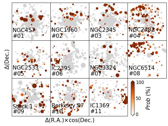
Figure 1: Sky charts of stars with assigned membership probability (Prob) higher than 50 per cent projected on the field of known open clusters (gray symbols) and XDOCCs (coloured symbols), respectively. The size of the symbols is proportional to the star brightness. Each panel, centred on the known open cluster, indicates its name and the number of the XDOCC.

Looking at their stellar distributions in the Galactic coordinate system (see Figures 9-11 in Jaehnig et al., 2021), most of the XDOCCs do not show the expected King (1962) profile (Piskunov et al., 2007; Kharchenko et al., 2013), but stars scattered across the analyzed field. This appearance led us to remind that field stars may also distribute in the CMD giving the appearance of the star sequence of an open cluster, as Burki & Maeder (1973) shown. Therefore, the presence of star sequences in CMDs should not be taken as a direct proof of the existence of a real open cluster. Relatively faint field star Main Sequences, for example, can mimic the lower part of open cluster Main Sequences. Precisely, the aim of this work consists in revisiting the 11 XDOCCs and providing with an assessment on their nature as genuine open clusters. The present results highlight the importance of considering not only the proper motions distribution to conclude on the existence of a physical system, but also, its spatial distribution, size, mass, etc.

In Section 2 we estimate XDOCC fundamental parameters disentangling observational errors from the intrinsic dispersion and compare the resulting values with those derived by Jaehnig et al. (2021). We also discuss different astrophysical aspects that arise from considering the available data to conclude on the unsupported existence of new open clusters. In Section 3 we summarize the main conclusions of this work and suggest some sanity check analysis for future searches of open cluster candidates.

2 Data analysis and discussion

For comparison purposes with the work by Jaehnig et al. (2021), we employed their same data sets, which include stars with assigned membership probabilities higher than 50 per cent. Since the 11 XDOCCs were identified projected on the field of 11 known open clusters, we also retrieved the same information for them. We started by constructing schematic sky charts for the 11 XDOCCs, which we depict in Fig. 1. Stars of the known open clusters were drawn with light gray filled circles and those of the 11 XDOCCs with coloured ones, according to their membership probability. We represented the stars with circles of different size, which are proportional to the star brightness. Each panel is centred on the known open cluster and its size is such that it includes all the retrieved stars in the field. At first glance, the known open clusters are clearly visible, with the sole exception of NGC 6514 (middle-right panel), which is a diffuse nebula known as the "Trifid" Nebula (Glushkov & Karyagina, 1984). As for the 11 XDOCCs, their appearance do not seem to resemble those of real open clusters, with some exceptions. Indeed, although open clusters can have stars spatially sparsely distributed in comparison with those in globular clusters, they all have a core (central) region of higher stellar density. Open clusters also usually show brighter stars more centrally concentrated than fainter stars. Based on these qualitative descriptions of an open cluster, we distinguished those XDOCCs with a chance of being real stellar aggregates from those that seem more probably to be the result of a superposition of stars aligned along the line-of.sight. We included such a classification in Table 1 with an Y or N, respectively.

2.1 Stellar mass functions

Joshi et al. (2016) derived a relationship between open cluster mass and size that we used to probe the reality of the 11 XDOCCs as physical systems. By assuming that they are open clusters, we first constructed their mass functions from which we estimated an upper limit for their initial total masses. In order to do that, we used stars with membership probabilities higher than 50 and 90 per cent, respectively, with the aim of evaluating mass function uncertainties. While counting the number of stars per mass interval, we adopted a mass bin of log($M$ /M_⊙) = 0.05. The individual stellar masses were interpolated using the theoretical isochrones computed by Bressan et al. (2012, PARSEC v1.2S), the Gaia $G$ magnitudes and the ages, distances and interstellar absorptions $A_{V}$ derived for the 11 XDOCCs by Jaehnig et al. (2021). The resulting mass functions are shown in Fig. 2, where we distinguished with black and orange open clusters those built for stars with membership probabilities higher than 50 and 90 per cent, respectively. As can be seen, there is only small differences between them. We then matched on them a Kroupa (2002)’s mass function profile, which in turn we used to compute the total mass for stars more massive than 0.5M_⊙. We then computed the XDOCCs’ Jacobi radii using the expression (Spitzer, 1987):

$$R_{J}=\left(\frac{M_{XDOCC}}{3M_{MW}}\right)^{1/3}\times R_{GC}$$ (1)

where $M_{XDOCC}$ is the XDOCC’s mass derived above and $M_{MW}$ is the Milky Way mass comprised within a radius equal to the XDOCC’s Galactocentric distance ($R_{GC}$). The $R_{GC}$ values were taken from Jaehnig et al. (2021), while $M_{MW}$ values were interpolated in the Milky Way mass versus Galactocentric relationship obtained by (Bird et al., 2022). We obtained two different $R_{J}$ values using the derived XDOCC’s mass estimates for membership probabilities higher than 50 and 90 per cent, respectively. We included these values as labels in the different panels of Fig. 3.

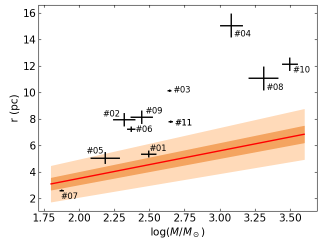
Figure 4: Relationship between radii and masses of the 11 XDOCCs. The red line, and orange and light-red shaded regions around it represent the relationship derived by Joshi et al. (2016) and the 1$\sigma$ and 3$\sigma$ confidence intervals, respectively. The numbers of the respective XDOCCs are also indicated.

The resulting $M_{XDOCC}$ and $R_{J}$ ranges were plotted in Fig. 4 as horizontal and vertical segments, respectively, where we also included the radius versus mass relationship obtained by Joshi et al. (2016). We used the locci of the XDOCCs in Fig. 4 as an additional criterion for assessing on their physical reality as open clusters. Particularly, objects that fall within a 3$\sigma$ confidence interval (XDOCC 01, 05, and 07) were considered as possible real systems, and for them, we included an Y in Table 1.

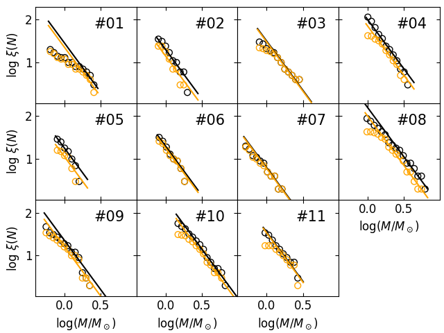
Figure 2: Mass function of the XDOCCs, with the corresponding numbers labeled in the respective panels. Black and orange circles correspond to mass functions built from stars with membership probabilities higher than 50 and 90 per cent, respectively. The coloured straight lines match the respective mass distributions.

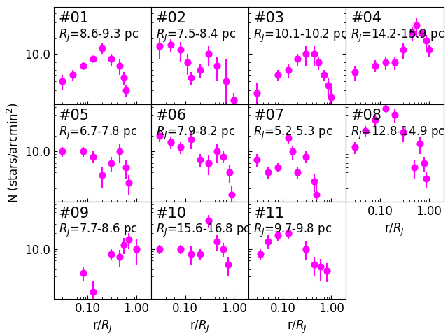
Figure 3: Stellar number density profiles of the XDOCCs, with the corresponding numbers labeled in the respective panels. The derived Jacobi radius ranges are also indicated (see text for details).

2.2 Stellar number density profiles

In order to quantify the visual appearance of the 11 XDOCCs (see Fig. 1), we built their stellar number density profiles. To to this, we counted the number of stars in annuli centred on the XDOCCs of width 0.050, 0.067, 0.100, and 0.200 times their Jacobi radii (for membership probabiilties higher than 90 per cent), respectively, and then averaged all the obtained density values, previously rebinned from interpolation, and computed their standard errors. The resulting binned number density profiles are shown in Fig. 3, where we used the ratio between the distance to the XDOCC’s centre and the Jacobi radius for comparison purposes. In addition, dealing with $R_{J}$ values allow us to evaluate the level of star mass segregation and to probe whether there are unbound stars among those identified as XDOCCs’ members (Küpper et al., 2010). The latter is an interesting aspect to analyze given the sparse appearance of the 11 XDOCCs.

The stellar radial profile of an open cluster is expected to follow a King’s (King, 1962) model (Piskunov et al., 2007; Kharchenko et al., 2013, and references therein), as follows:

$$f(r)=k\times\left(\frac{1}{\sqrt{1+(r/r_{c})^{2}}}-\frac{1}{\sqrt{1+(r_{t}/r_{c})^{2}}}\right)^{2},$$ (2)

where $k$ is a constant, $r_{c}$ and $r_{t}$ are the core and tidal radius, respectively. Eq. (2) implies that there is not any clusters’ members beyond $r_{t}$. Likewise, $r_{t}$ cannot be larger than the derived $R_{J}$. Recently, Zhong et al. (2022) showed that a two-components model with a King core distribution and a logarithmic Gaussian outer halo distribution describe better the internal and external structural features of open clusters. They found that core, half-mass, tidal and Jacobi radii are statistically linearly related, which suggests that the inner and outer regions of the clusters are interrelated and follow similar evolutionary processes. Because none of the XDOCCs’ number density profiles of Fig. 3 resembles a King’s (King, 1962) profile, we concluded that the XDOCCs are not real open clusters, and included an N in the fourth column of Table 1. Note that the remarkable drop of the stellar number density profiles towards the inner regions is not caused by crowding effects, because XDOCCs are composed by a relatively sparse group of stars.

Table 1: Assessments on the reality of XDOCCs as open clusters.

Name	sky chart	size and mass	radial profile	CMD	adopted
XDOCC-01	N	Y	N	N	N
XDOCC-02	N	N	N	N	N
XDOCC-03	N	N	N	N	N
XDOCC-04	N	N	N	N	N
XDOCC-05	N	Y	N	N	N
XDOCC-06	Y	N	N	N	N
XDOCC-07	N	Y	N	N	N
XDOCC-08	Y	N	N	N	N
XDOCC-09	N	N	N	N	N
XDOCC-10	N	N	N	N	N
XDOCC-11	Y	N	N	N	N

2.3 Colour-magnitude diagrams

We first obtained individual stellar reddenings through the GALExtin interface (Amôres et al., 2021), by using the Milky Way reddening map of Chen et al. (2019), which was built specifically for Gaia bandpasses. We then corrected the $G$ magnitudes and $BP-RP$ colours using the retrieved total absorptions ($A_{G}$) and the total to selective absorption ratios given by Chen et al. (2019). The absorption uncertainties $\sigma$($A_{G}$) span from 0.003 up to 0.020 mag, with an average of 0.010 mag at any $A_{G}$ interval. Fig. 5 illustrates the spatial reddening variations for the XDOCCs’ stars, with stars coloured according to their $E(B-V)$ values, while Fig. 6 depicts the reddening corrected CMDs.

We performed isochrone fits to the reddening corrected XDOCCs’ CMDs, not assuming a solar metallicty (Jaehnig et al., 2021), but including the metallicity ([M/H]), the age, the total mass, and the binary fraction as free parameters. The fundamental parameters were derived by employing specific routines of the Automated Stellar Cluster Analysis code (ASteCA, Perren et al., 2015), which is able to derive them simultaneously. ASteCA relies on the construction of a large number of synthetic CMDs from which it finds the one which best resembles the observed CMD. Thus, the metallicity, the age, the distance, the reddening, the star cluster present mass and the binary fraction associated to that best representative generated synthetic CMD are adopted as the best-fitted star cluster properties.

ASteCA is able to handle with a wide range of values of the aforementioned parameters. However, since the stars used share similar parallaxes (see Table 1 and Figures 9-11 in Jaehnig et al., 2021), we constrained the generation of synthetic CMDs to those with distance modulus around the mean observed parallaxes. We fitted theoretical isochrones computed by Bressan et al. (2012, PARSEC) for the Gaia DR2 photometric system. Particularly, we chose PARSEC v1.2S isochrones spanning metallicities ($Z$ = 0.0152$\times$10^[Fe/H]) from 0.003 dex up to 0.038 dex, in steps of 0.001 dex and log(age /yr) from 7.0 up to 9.0 in steps of 0.025. Because photometric errors are not include in Table 2 of Jaehnig et al. (2021), we interpolated them from Figures 9-11 in Evans et al. (2018). To derive the errors in the Gaia colour, we added in quadrature those of the individual involved magnitudes. We note that reliable photometric uncertainties are needed to uncover the intrinsic dispersion in the CMD. If points in the CMD are used without errors then, the observed scatter is considered as the result of the combined intrinsic dispersions of the fundamental parameters (reddening, distance, age, etc). When photometry errors are taken into account, then the resulting astrophysical properties uncertainties are better constrained. In practice, the intrinsic dispersion should be smaller than observed photometric ones.

ASteCA generates synthetic CMDs by adopting the initial mass function given by Kroupa (2002) and a minimum mass ratio for the generation of binaries of 0.5. The total observed star cluster mass and its binary fraction were set in the ranges 100-5000 M_⊙ and 0.0-0.5, respectively. In brief, ASteCA explores the parameter space of the synthetic CMDs through the minimization of the likelihood function defined by Tremmel et al. (2013, the Poisson likelihood ratio (eq. 10)) using a parallel tempering Bayesian MCMC algorithm, and the optimal binning Knuth (2018)’s method. The uncertainties associated to the derived parameters are estimated from the standard bootstrap method described in Efron (1982). We refer the reader to Perren et al. (2015) where details related to the implementation of these algorithms are provided. The resulting fundamental parameters are listed in Table 2 and the object CMDs with the isochrone corresponding to those parameter values are illustrated in Fig. 6.

Table 2: ASteCA results for XDOCC objects

Name	log($t$ /yr)	[Fe/H]	Mass	binary
		(dex)	(M⊙)	fraction
XDOCC-01	8.13$\pm$0.28	0.40$\pm$0.20	213$\pm$89	0.38$\pm$0.14
XDOCC-02	7.47$\pm$0.43	0.24$\pm$0.18	343$\pm$122	0.45$\pm$0.12
XDOCC-03	7.23$\pm$0.48	0.25$\pm$0.24	189$\pm$93	0.17$\pm$0.13
XDOCC-04	8.47$\pm$0.06	0.23$\pm$0.12	1543$\pm$328	0.32$\pm$0.10
XDOCC-05	7.73$\pm$0.45	0.17$\pm$0.19	188$\pm$126	0.22$\pm$0.15
XDOCC-06	7.67$\pm$0.40	0.39$\pm$0.15	229$\pm$123	0.41$\pm$0.12
XDOCC-07	8.76$\pm$0.31	0.24$\pm$0.24	125$\pm$38	0.43$\pm$0.13
XDOCC-08	8.75$\pm$0.12	0.34$\pm$0.12	661$\pm$304	0.40$\pm$0.12
XDOCC-09	8.71$\pm$0.26	0.07$\pm$0.19	204$\pm$82	0.35$\pm$0.13
XDOCC-10	8.85$\pm$0.08	0.40$\pm$0.17	655$\pm$288	0.29$\pm$0.12
XDOCC-11	8.48$\pm$0.37	0.37$\pm$0.15	591$\pm$165	0.29$\pm$0.14

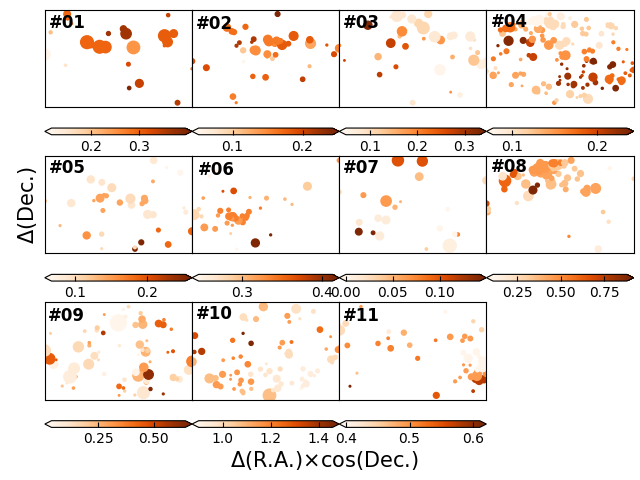
Figure 5: Sky charts of XDOCCs’ stars (see Fig. 1); the size of the symbols is proportional to the star brightness. Stars are coloured according the its $E(B-V)$ value (mag) as shown in the respective colour bar.

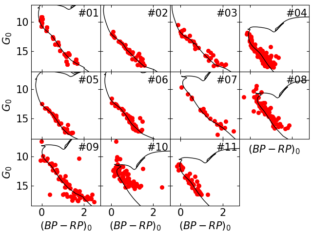
Figure 6: Reddening corrected Gaia CMDs of the 11 XDOCCs as labelled in the upper-right corner of the panels. The theoretical isochrone of Bressan et al. (2012, PARSEC v1.2S) corresponding to the parameters given in Table 2 and for the mean observed parallaxes derived by Jaehnig et al. (2021) are superimposed.

Fig. 6 shows relatively populated to very populous Main Sequences that extend from $\sim$ 4 up to $\sim$ 8 mag long. They do not show any clear sign of evolution, with the exception of the presence of few stars at the Main Sequence turn-off of XDOCC-08. Although the best representative isochrones satisfactorily reproduce these long Main Sequences, there is no star in more evolved stellar evolutionary phases, as we expect in open clusters with populous Main Sequences. Indeed, by using the Padova group web interface, we generated synthetic CMDs of open clusters having the total masses, ages and metallicities derived for the 11 XDOCCs and found that they show 1-2 red clump stars and very well populated Main Sequence turn-off regions.

As Burki & Maeder (1973) shown, a composite star field population can mimic in the CMD the appearance of an open cluster’s star sequence. Disentangling whether this is the case of the XDOCCs’ CMDs (Fig. 6) is difficult to accomplish only from the analysis of those CMDs. However, because of the minimization of likelihood functions used to derive the astrophysical parameters, the derived bootstrapped uncertainties tell us about the level of uniqueness of the representative solutions. Thus, under the presence of relatively tight Main Sequences and small photometric errors, relatively large parameter uncertainties could suggest that different collections of isochrones are needed to map different parts of the observed Main Sequence. When dealing with true open clusters, typical intrinsic dispersions of fundamental parameters as estimated by ASteCA (Perren et al., 2022, and references therein) are $\sigma$log($t$ /yr) $\approx$ 0.12, and $\sigma$[Fe/H] $\approx$ 0.21 dex. Table 2 shows that age uncertainties are notably large in most of the cases, suggesting that a range of ages represent the fitted Main Sequences. The resulting metallicities are also notably larger than the values of open clusters that follow the metallicity gradient of the Milky Way disk. We used the Galactocentric distances of XDOCCs computed by Jaehnig et al. (2021), the recently age-metallicity-Galactocentric position relationship derived by Magrini et al. (2022) from the Gaia-ESO survey (Gilmore et al., 2012), and ages and metallicities of Table 2, to confirm that all XDOCCs fall outside the relationship for open clusters. Finally, the resulting binary fractions (see Table 2) generated by ASteCA are relatively high. This happens when the wider broadness of the Main Sequence of a composite star field population is assumed to be the Main Sequence of a star cluster.

2.4 Spectroscopic data

Chemical abundances and radial velocities for individual stars are also helpful in order to disentangle whether they belong to the field population or to a stellar aggregate. We took advantage of the Sloan Digital Sky Survey (SDSS) IV DR17, particularly the APOGEE-2 database (Blanton et al., 2017; Ahumada et al., 2020), to retrieve this information. The spectral parameters provided in the APOGEE-2 database were obtained using the APOGEE Stellar Parameters and Chemical Abundance Pipeline (ASPCAP; García Pérez et al., 2016) and were accessed employing the following Structured Query Language (SQL) query to the SDSS database server :

SELECT TOP 100

s.apogee$\_$id,s.ra,s.dec,s.glon,s.glat,s.snr,

s.vhelio$\_$avg,s.verr,a.teff,a.teff$\_$err,a.logg,

a.logg$\_$err,a.m$\_$h,a.m$\_$h$\_$err,a.alpha$\_$m,

a.alpha$\_$m$\_$err

FROM apogeeStar as s

JOIN aspcapStar a on s.apstar$\_$id = a.apstar$\_$id

JOIN dbo.fGetNearbyApogeeStarEq(RA,DEC,20) as

near on a.apstar_id=near.apstar_id

WHERE (a.aspcapflag & dbo.fApogeeAspcapFlag

(’STAR_BAD’)) = 0

We then cross-matched the retrieved APOGEE-2 data sets for the 11 XDOCCs with the corresponding Gaia data sets using RA and Dec coordinates as matching variables and Astropy Project tools. We found only one star in common for XDOCCs 10 (2057948152709390848 (Gaia DR2 name) == 2M20223036+3712003 (APOGEE-2 name)) with $T_{eff}$ = (16187.49$\pm$647.53)^oK, log($g$)=4.252$\pm$0.082, and radial velocity = (-18.41$\pm$2.43) km/s. No metallicity information is available. By using the derived age, distance, and interstellar absorption of XDOCCs 10 (Jaehnig et al., 2021), we found by interpolation into the corresponding theoretical isochrone that the Gaia DR2 magnitude and colour resulted to be $G$=14.16$\pm$0.30 mag and $BP-RP$ = 1.38$\pm$0.15 mag, respectively. These values differ significantly from the observed ones, namely, $G$ = 14.654 mag and $BP-RP$ = 2.048 mag. Therefore, we concluded that the star is not at the mean distance of XDOCC 10, although its position in the CMD suggests otherwise. This result points to the need of further spectroscopic data to assess on the physical nature of the 11 XDOCCs. We also note that the individual Gaia DR2 parallax uncertainties of the stars selected as members of these objects are still large as to secure a reliable analysis of their distances, and hence a 3D structural study of them. With accurate parallaxes, the 3D XDOCCs’ dimensions could be estimated and from them, a comparison with the known size range of real open clusters could be carried out.

3 Concluding remarks

The number of open cluster candidates identified since recent time from the availability of public databases and computer-based searching techniques is steadily increasing. Likewise, these data sets and analysis methods have been helpful to improve the accuracy of open clusters’ fundamental parameters that are re-determined from an homogeneous basis. The outcomes of this promising effort certainly help us to improve our knowledge of the Milky Way open cluster system, and hence to better understand the formation and evolution of the disc of our Galaxy.

Recently, Jaehnig et al. (2021) used Gaia DR2 data sets to determine the astrophysical properties of 420 known open clusters, by employing extreme deconvolution gaussian mixture models. They also pointed out that other previously unknown 11 open cluster candidates could be populating the searched sky regions. The identification of these new candidates mainly relies on stellar overdensities detected in the Vector Point diagram, whose stars are distributed in CMDs following the appearance of those typical of open clusters; the distribution of parallaxes also turned out to be at first glance compatible with stars being at a similar mean distance. Nevertheless, Jaehnig et al. (2021) stressed that further investigations are necessary in order to confirm their physical nature.

By using the same data sets, we carried out a thorough analysis of these new open cluster candidates (XDOCCs), from which we identified a number of astrophysical aspects that do not fully agree with our present knowledge of the open cluster population. These considerations come from our independent estimates of age, reddening, metallicity, total mass, and binary fraction of the 11 XDOCCs, considering them as real physical stellar systems. These fundamental parameters were derived by disentangling their intrinsic dispersions from the photometric data sets uncertainties. We obtained astrophysical properties whose associated dispersions are much larger than those usually obtained for open clusters using the same procedure. Such large dispersions are typical of fundamental parameters of composite star field populations.

The apparent distribution of stars in the sky, their projected stellar number density profiles, and the relationship between their masses and projected radii support also that, considered all together, the conclusion that the XDOCCs unlikely are real physical systems. We think that this finding highlights the need of gathering more than one criterion when searching for open cluster candidates. Here we show that a stellar overdensity in the proper motion space is not enough to conclude on the existence of a stellar aggregate. By relying on a multidimensional approach (3D positions, 3D motions, metallicity, CMD features, etc) more confidence open cluster candidates will be uncovered. Nevertheless, because of the clearly observed gathering of stars in the Vector Point diagram and some hint for similar distances within the Gaia DR2 parallax uncertainties, the XDOCCs could be considered like sparse groups of stars.

4 Data availability

Data used in this work are available upon request to the author.

References

- Ahumada et al. (2020) Ahumada R., et al., 2020, ApJS, 249, 3
- Amôres et al. (2021) Amôres E. B., et al., 2021, MNRAS, 508, 1788
- Anders et al. (2021) Anders F., Cantat-Gaudin T., Quadrino-Lodoso I., Gieles M., Jordi C., Castro-Ginard A., Balaguer-Núñez L., 2021, A&A, 645, L2
- Astropy Collaboration et al. (2013) Astropy Collaboration et al., 2013, A&A, 558, A33
- Astropy Collaboration et al. (2018) Astropy Collaboration et al., 2018, AJ, 156, 123
- Astropy Collaboration et al. (2022) Astropy Collaboration et al., 2022, ApJ, 935, 167
- Babusiaux et al. (2022) Babusiaux C., et al., 2022, arXiv e-prints, p. arXiv:2206.05989
- Bird et al. (2022) Bird S. A., et al., 2022, MNRAS,
- Blanton et al. (2017) Blanton M. R., et al., 2017, AJ, 154, 28
- Bressan et al. (2012) Bressan A., Marigo P., Girardi L., Salasnich B., Dal Cero C., Rubele S., Nanni A., 2012, MNRAS, 427, 127
- Burki & Maeder (1973) Burki G., Maeder A., 1973, A&A, 25, 71
- Cantat-Gaudin et al. (2020) Cantat-Gaudin T., et al., 2020, A&A, 640, A1
- Castro-Ginard et al. (2021) Castro-Ginard A., et al., 2021, arXiv e-prints, p. arXiv:2111.01819
- Chen et al. (2019) Chen B. Q., et al., 2019, MNRAS, 483, 4277
- Dias et al. (2021) Dias W. S., Monteiro H., Moitinho A., Lépine J. R. D., Carraro G., Paunzen E., Alessi B., Villela L., 2021, MNRAS, 504, 356
- Efron (1982) Efron B., 1982, The Jackknife, the Bootstrap and other resampling plans
- Evans et al. (2018) Evans D. W., et al., 2018, A&A, 616, A4
- Gaia Collaboration et al. (2016) Gaia Collaboration et al., 2016, A&A, 595, A1
- Gaia Collaboration et al. (2018) Gaia Collaboration et al., 2018, A&A, 616, A1
- García Pérez et al. (2016) García Pérez A. E., et al., 2016, AJ, 151, 144
- Gilmore et al. (2012) Gilmore G., et al., 2012, The Messenger, 147, 25
- Glushkov & Karyagina (1984) Glushkov Y. I., Karyagina Z. V., 1984, Trudy Astrofizicheskogo Instituta Alma-Ata, 44, 43
- Hunt & Reffert (2021) Hunt E. L., Reffert S., 2021, A&A, 646, A104
- Ivanov et al. (2017) Ivanov V. D., Piatti A. E., Beamín J.-C., Minniti D., Borissova J., Kurtev R., Hempel M., Saito R. K., 2017, A&A, 600, A112
- Jadhav et al. (2021) Jadhav V. V., Roy K., Joshi N., Subramaniam A., 2021, AJ, 162, 264
- Jaehnig et al. (2021) Jaehnig K., Bird J., Holley-Bockelmann K., 2021, ApJ, 923, 129
- Joshi et al. (2016) Joshi Y. C., Dambis A. K., Pandey A. K., Joshi S., 2016, A&A, 593, A116
- Kharchenko et al. (2013) Kharchenko N. V., Piskunov A. E., Schilbach E., Röser S., Scholz R. D., 2013, A&A, 558, A53
- King (1962) King I., 1962, AJ, 67, 471
- Knuth (2018) Knuth K. H., 2018, optBINS: Optimal Binning for histograms (ascl:1803.013)
- Kroupa (2002) Kroupa P., 2002, Science, 295, 82
- Küpper et al. (2010) Küpper A. H. W., Kroupa P., Baumgardt H., Heggie D. C., 2010, MNRAS, 407, 2241
- Magrini et al. (2022) Magrini L., et al., 2022, arXiv e-prints, p. arXiv:2210.15525
- Minniti et al. (2010) Minniti D., et al., 2010, New Astron., 15, 433
- Nidever et al. (2021) Nidever D. L., et al., 2021, AJ, 161, 74
- Pavani et al. (2011) Pavani D. B., Kerber L. O., Bica E., Maciel W. J., 2011, MNRAS, 412, 1611
- Perren et al. (2015) Perren G. I., Vázquez R. A., Piatti A. E., 2015, A&A, 576, A6
- Perren et al. (2022) Perren G. I., Pera M. S., Navone H. D., Vázquez R. A., 2022, arXiv e-prints, p. arXiv:2204.02153
- Piskunov et al. (2007) Piskunov A. E., Schilbach E., Kharchenko N. V., Röser S., Scholz R. D., 2007, A&A, 468, 151
- Spitzer (1987) Spitzer L., 1987, Dynamical evolution of globular clusters
- Torrealba et al. (2019) Torrealba G., Belokurov V., Koposov S. E., 2019, MNRAS, 484, 2181
- Tremmel et al. (2013) Tremmel M., et al., 2013, ApJ, 766, 19
- Zhong et al. (2022) Zhong J., Chen L., Jiang Y., Qin S., Hou J., 2022, AJ, 164, 54