Learning Integrable Dynamics with Action-Angle Networks

Abstract

Machine learning has become increasingly popular for efficiently modelling the dynamics of complex physical systems, demonstrating a capability to learn effective models for dynamics which ignore redundant degrees of freedom. Learned simulators typically predict the evolution of the system in a step-by-step manner with numerical integration techniques. However, such models often suffer from instability over long roll-outs due to the accumulation of both estimation and integration error at each prediction step. Here, we propose an alternative construction for learned physical simulators that are inspired by the concept of action-angle coordinates from classical mechanics for describing integrable systems. We propose Action-Angle Networks, which learn a nonlinear transformation from input coordinates to the action-angle space, where evolution of the system is linear. Unlike traditional learned simulators, Action-Angle Networks do not employ any higher-order numerical integration methods, making them extremely efficient at modelling the dynamics of integrable physical systems.

1 Introduction

1.1 Modelling Hamiltonian Systems

Hamiltonian systems are an important class of physical systems whose dynamics are governed by a scalar function $H$, called the Hamiltonian. The state of a Hamiltonian system is a 2-tuple $u(t)=(q(t),p(t))$, where $q\in\mathbb{R}^{n}$ are the positions and $p\in\mathbb{R}^{n}$ are the canonical momenta. We are interested in predicting the time evolution of a Hamiltonian system as a function of time $t$. In particular, we seek to learn a model ${\mathcal{M}}_{\phi}$ (parameterized by $\phi$) that can accurately predict the future state $u(t+\Delta t)$ given the current state $u(t)$:

$${\mathcal{M}}_{\phi}(u(t),\Delta t)\approx u(t+\Delta t).$$ (1)

Previous efforts towards modelling Hamiltonian systems (Greydanus et al., 2019; Cranmer et al., 2020; Jin et al., 2020; Chen et al., 2018; Kidger, 2022) have seen success with neural networks trained via backpropagation on the trajectory prediction objective:

$$\phi^{*}=\operatorname*{arg\,min}_{\phi}\ \sum_{t}\lVert{\mathcal{M}}_{\phi}(u(t),\Delta t)-u(t+\Delta t))\rVert^{2}.$$

Such models are often constrained in some way to match the underlying physical evolution, which improves their accuracy. However, they suffer from several drawbacks that have restricted their effectiveness: (1) Their predictions tend to be unstable over long roll-outs (when $\Delta t$ is large). (2) They tend to require many parameters and need long training times. Further, the inference times of these models often scale with $\Delta t$.

Based on the principle of action-angle coordinates (Vogtmann et al., 1997) from classical mechanics, we introduce a new paradigm for learning physical simulators which incorporate an inductive bias for learning integrable dynamics. Our Action-Angle Network learns an invertible transformation to action-angle coordinates to linearize the dynamics in this space. In this sense, the Action-Angle Network can be seen as a physics-informed adaptation of DeepKoopman (Lusch et al., 2018). The Action-Angle Network is efficient both in parameter count and inference cost; it requires much fewer parameters than previous methods to reach similar performance and enjoys an inference time independent of $\Delta t$.

1.2 Action-Angle Coordinates

The time evolution of any Hamiltonian system is given by Hamilton’s equations:

$$\frac{dq}{dt}=\frac{\partial H}{\partial p},\quad\frac{dp}{dt}=-\frac{\partial H}{\partial q}\vspace{-0.5em}$$ (2)

where $H$ is the Hamiltonian of the system. The complexity for learning these dynamics arises solely because $H$ is not known and must be inferred; only samples from a trajectory over which $H$ is conserved is available. The core issue for all physical simulators is the non-linearity of the dynamics when expressed in the canonical coordinates $(q,p)$. However, for integrable systems (Tong, 2004) which possess significant symmetry, the dynamics are actually linear in a set of coordinates termed the action-angle coordinates (Vogtmann et al., 1997). The actions $I$ and angles $\theta$ are related to the canonical coordinates $(q,p)$ via a symplectic transformation ${\mathcal{T}}$ (Meyer and Hall, 2013) as $(I,\theta)={\mathcal{T}}(q,p)$. In the action-angle coordinates, the Hamiltonian only depends on the actions $I$, not the angles $\theta$. Thus, Hamilton’s equations in this basis tell us that:

$$\frac{dI}{dt}=-\frac{\partial H}{\partial\theta}=0,\quad\frac{d\theta}{dt}=\frac{\partial H}{\partial I}.$$ (3)

Thus, the actions $I$ are always constant across a trajectory, while the angles evolve linearly with constant rate $\dot{\theta}=\frac{\partial H}{\partial I}$. The action-angle space can be thought of as a torus $\mathbb{T}^{n}$, where the actions $I$ are a function of the radii, and the angles describe the individual phases living in $[0,2\pi)$.

Learning the mapping ${\mathcal{T}}$ from canonical coordinates $(q,p)$ to action-angle coordinates $(I,\theta)$ for several physical systems was first explored in (Bondesan and Lamacraft, 2019), which did not focus on the complete dynamics of integrable systems. We leverage their framework to additionally incorporate a dynamics model ${\mathcal{F}}$ to learn a complete physical simulator.

Ishikawa et al. (2021) attempt to model the time evolution of actions for integrable systems by learning the Hamiltonian in action-angle coordinates. However, their overall objective and training setup are different from ours: they have samples of the true action-angle coordinates $(I,\theta)$ as input, while we only observe the canonical coordinates $(q,p)$.

2 Action-Angle Networks

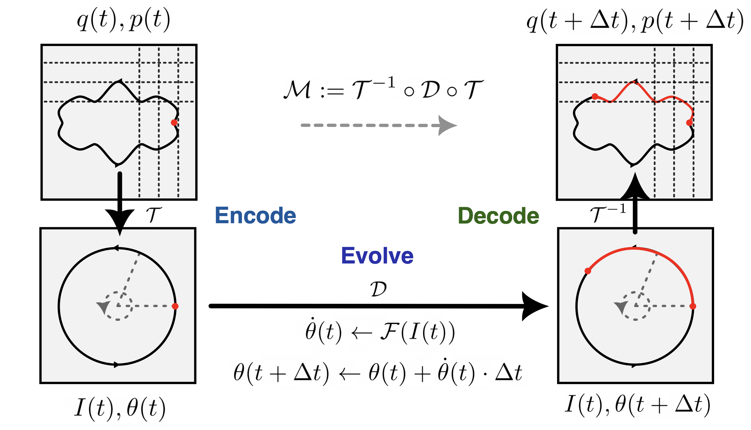
Figure 1: An overview of the Action-Angle Network.

Suppose we observe the system at time $t$, and we query our model ${\mathcal{M}}_{\phi}$ to predict the state at a future time $t+\Delta t$. The Action-Angle Network performs the following operations, illustrated in Figure 1:

• Encode: Convert the current state in canonical coordinates $q(t),p(t)$ to action-angle coordinates $I(t),\theta(t)$ via a learned map ${\mathcal{T}}$.

• Evolve: Compute the angular velocities $\dot{\theta}(t)$ at this instant with the dynamics model ${\mathcal{F}}$:
  $\dot{\theta}(t)\leftarrow{\mathcal{F}}(I(t))$. Evolve the angles to time $t+\Delta t$ with these angular velocities:

  $$\theta(t+\Delta t)\leftarrow\theta(t)+\dot{\theta}(t)\cdot\Delta t\pmod{2\pi}$$ (4)

• Decode: Convert the new state back to canonical coordinates $q(t+\Delta t),p(t+\Delta t)$ via ${\mathcal{T}}^{-1}$.

Symplectic Normalizing Flows: The transformation ${\mathcal{T}}$ from canonical coordinates to action-angle coordinates is guaranteed to be symplectic (Vogtmann et al., 1997). To constrain our encoder to learn only symplectic transformations, we compose layers of symplectic normalizing flows (Li et al., 2020; Bondesan and Lamacraft, 2019; Jin et al., 2020). In particular, we found that the G-SympNet layers (Jin et al., 2020) with our modification described below performed well empirically. G-SympNet was shown to be universal; they can represent any symplectic transformation given sufficient width and depth. Similar to affine coupling layers (Dinh et al., 2014), each G-SympNet layer $\psi_{i}$ operates on only one of the coordinates keeping the other fixed, depending on the parity of $i$:

$$\psi_{2k}(q,p)=(q,p+f(q)),\quad\psi_{2k+1}(q,p)=(q+f(p),p)$$ (5)

where $f$ is of the following form $f(x)=Cx+W^{T}\text{diag}(A)\sigma(Wx+B)$ with learnable parameters $A\in\mathbb{R}^{d_{o}},B\in\mathbb{R}^{d_{o}},C\in\mathbb{R}$ and $W\in\mathbb{R}^{d_{o}\times n}$, where $d_{o}$ is a hyperparameter. Our minor modification above allows each layer to model the identity transformation, enabling the training of deeper models.

Action-Angles via Polar Coordinates: We found that learning a mapping from canonical coordinates which live in $\mathbb{R}^{2n}$ directly to action-angle coordinates which live in the torus $\mathbb{T}^{n}$ was challenging for the network. We hypothesize that the differing topology of these spaces is a major obstacle because of the resulting singularities. To bypass this, we borrow a trick from Bondesan and Lamacraft (2019); we have the G-SympNet instead output the components of the actions $(I^{(x)},I^{(y)})$ in the Cartesian coordinate basis. These are then converted to action-angles $(I,\theta)$ in the polar coordinate basis, by the standard transformation ${\mathcal{T}}_{\text{polar}}$ applied to each pair of $(I^{(x)}_{i},I^{(y)}_{i})$ coordinates:

$$I_{i}=\sqrt{(I^{(x)}_{i})^{2}+(I^{(y)}_{i})^{2}},\quad\theta_{i}=\arctan(I^{(y)}_{i}/I^{(x)}_{i})$$ (6)

Our encoder can thus be described as ${\mathcal{T}}:={\mathcal{T}}_{\text{Polar}}\circ\text{G-SympNet}$.

Evolve: From Equation 3, we know that the angular velocities $\dot{\theta}$ are only a function of the actions $I$ at the instant $t_{0}$, which we model as a simple multi-layer perceptron (MLP) ${\mathcal{F}}$. Since the angles $\theta$ are guaranteed to evolve linearly, we do not need to use higher-order numerical integration schemes. Instead, a single call to the forward Euler method is exact:

$$\dot{\theta}(t_{0}) \leftarrow{\mathcal{F}}(I(t_{0}))\quad\theta(t_{0}+\Delta t)\leftarrow\theta(t_{0})+\dot{\theta}(t_{0})\cdot\Delta t\pmod{2\pi}$$ (7)

Decode: As ${\mathcal{T}}$ is symplectic, ${\mathcal{T}}$ is invertible. Thus, our decoder is ${\mathcal{T}}^{-1}:=\text{G-SympNet}^{-1}\circ{\mathcal{T}}_{\text{polar}}^{-1}$.

2.1 Training

We generate a trajectory $\text{Tr}=\{(q(t),p(t))\}_{t=1}^{T}$ of $T=1000$ time steps, by either evaluating the closed-form dynamics equations or via numerical integration. In practise, this trajectory can also be obtained from raw observations, and does not need to be regularly sampled in time. We train models upto the first $500$ time steps and evaluate performance on the last $500$ time steps, for each trajectory.

State Prediction Error: We wish to learn parameters $\phi:=(\phi_{{\mathcal{T}}},\phi_{{\mathcal{F}}})$ that minimize the prediction loss $L_{\text{predict}}$:

$$L_{\text{predict}}=\textstyle\frac{1}{1+\Delta t}\textstyle\sum_{t_{0}\in\text{Tr}}\lVert{\mathcal{M}}_{\phi}(u(t_{0}),\Delta t)-u(t_{0}+\Delta t)\rVert^{2}.$$ (8)

Regularization of Predicted Actions: Additionally, we wish to enforce the fact that the predicted actions $I$ are constant across the trajectory. We do this by adding a regularizer $L_{\text{action}}$ on the variance of the predicted actions:

$$L_{\text{action}} =\textstyle\widehat{\mathrm{Var}}(I)=\frac{1}{T}\sum_{t_{0}\in\text{Tr}}\left(I(t_{0})-\widehat{\mathbb{E}}[I]\right)^{2}\text{where}\ \widehat{\mathbb{E}}[I]=\frac{1}{T}\sum_{t_{0}\in\text{Tr}}I(t_{0}).$$ (9)

We find that this global regularizer works better than the loss proposed in Bondesan and Lamacraft (2019) that minimizes only the local pairwise differences between the predicted actions across the trajectory. As the Action-Angle Network is completely differentiable, the parameters $\phi$ can be obtained via gradient-descent-based minimization of the total loss: $\phi^{*}=\text{argmin}_{\phi}\left(L_{\text{predict}}+\lambda L_{\text{action}}\right),$ where $\lambda$ is a hyperparameter that controls the strength of the regularization.

Schedule for $\Delta t$: Increasing $\Delta t$ over the course of training helped, as it corresponded to gradually increasing the complexity of the prediction task. We set $\Delta t_{\text{max}}=10$ and sampled $\Delta t$ according to:

$$\Delta t\sim\text{Uniform}\left(0,(\text{Current training step})/(\text{Maximum training steps})\right)\cdot\Delta t_{\text{max}}$$ (10)

3 Experiments

We compare the Action-Angle Network to three strong baseline models: the Euler Update Network (EUN), the Neural Ordinary Differential Equations (Neural ODE) (Chen et al., 2018), and the physics-inspired Hamiltonian Neural Networks (HNN) (Greydanus et al., 2019). A comparison of these models can be found in Table 1. The baseline models are further described in Section A.1.

Table 1: Comparing different models.

	Action-Angle Network	EUN	Neural ODE	HNN
Parameter count	$\approx 8.5$K	$\approx 9$K	$\approx 100$K	$\approx 200$K
Inference time	$O(1)$	$O(1)$	$O(\Delta t)$	$O(\Delta t)$
Learns conservation laws	✓			✓
Learns linear dynamics	✓	✓

As detailed in Section A.2, we simulate a system of coupled harmonic oscillators. Figure 2 depicts the prediction error for each of the models as a function of training samples, showing that the Action-Angle Network is much more data-efficient than the other baselines. 3(a) shows that the Action-Angle Network can be queried much faster than the Neural ODE and the HNN, with an inference time that is independent of $\Delta t$. 3(b) depicts the prediction error as a function of $\Delta t$, showing that the Action-Angle Network also scales much better with the jump size $\Delta t$, even for jump sizes larger than those seen during training $\Delta t_{\max}=10$. Finally, Figure 4 shows that the predicted angular frequencies from the Action-Angle Network closely match the true angular frequencies.

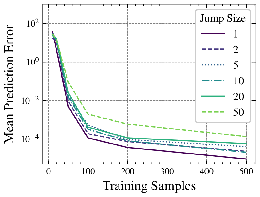
(a) Action-Angle Network

(b) Euler Update Network

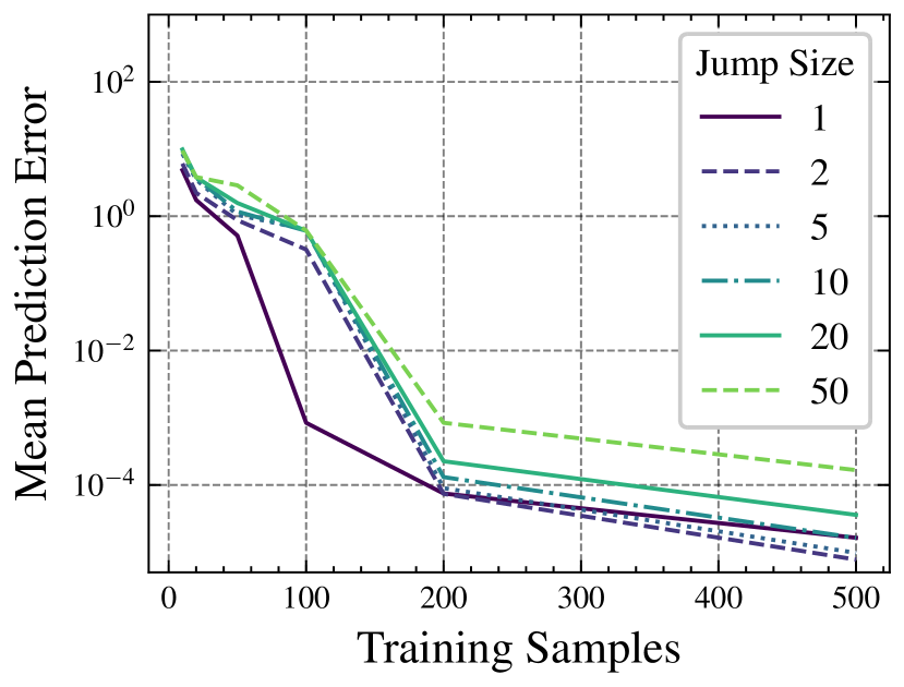
(c) Neural ODE

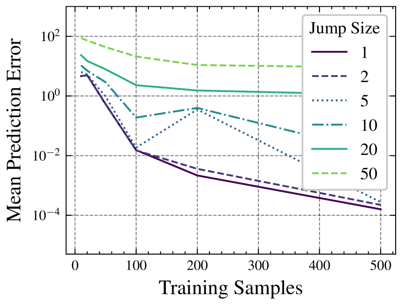
(d) Hamiltonian Neural Network

Figure 2: Prediction errors on test data as a function of training samples.

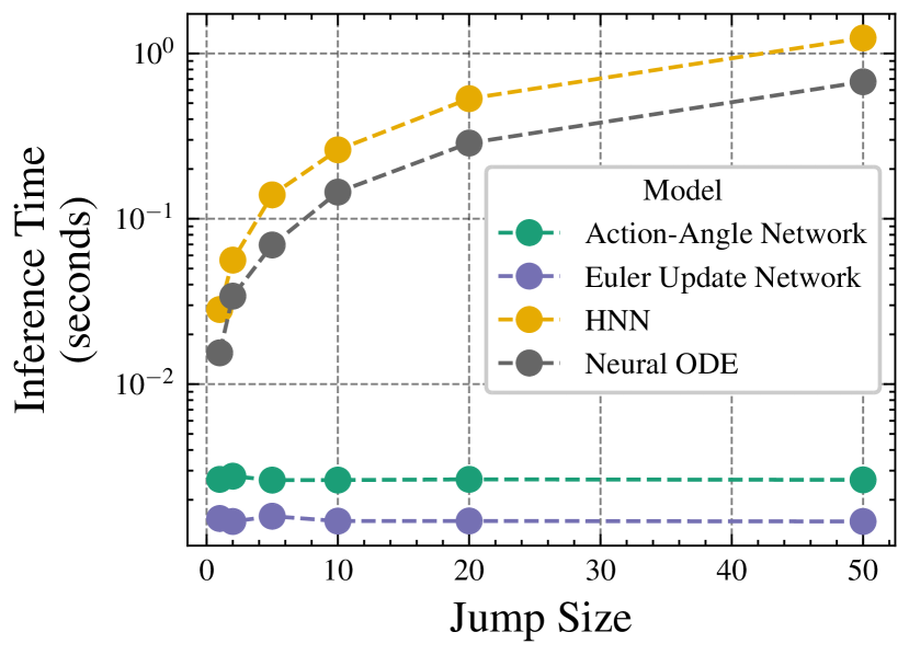
(a) Inference times as a function of jump $\Delta t$.

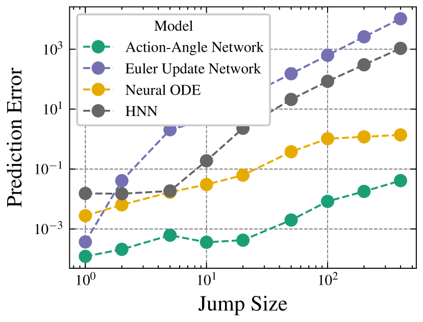
(b) Prediction error as a function of jump $\Delta t$.

Figure 3: Evaluating each model on (a) inference time and (b) prediction error.

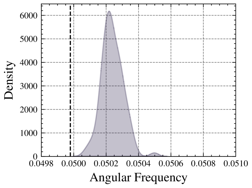
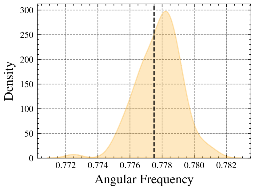
Figure 4: Kernel density plot of angular frequencies predicted by the Action-Angle Network. True angular frequencies are indicated by dashed vertical lines.

4 Conclusion

Our preliminary experiments indicate that Action-Angle Networks can be a promising alternative for learning efficient physical simulators. Action-Angle Networks overcome many of the obstacles – instability and inefficiency – faced by state-of-the-art learned simulators today. That being said, our experiments here only model very simple integrable systems. Next, we plan to analyse the performance of Action-Angle Networks on modelling large-scale non-integrable systems (such as cosmological simulations and molecular dynamics trajectories) to better understand their tradeoffs.

Broader Impact Statement

In this paper, we have proposed a novel method for modelling the dynamics of Hamiltonian systems, with improvements in computational efficiency. There has been much interest in accelerating simulations of various kinds across scientific domains that could have impact on human lives (for example, simulating biological cell cycles and immune system responses). However, given the techniques here apply to highly-constrained physical systems, we do not anticipate any negative social implications of our work.

Checklist

1. For all authors…

   1. Do the main claims made in the abstract and introduction accurately reflect the paper’s contributions and scope? [Yes] We have designed and evaluated Action-Angle Networks, showing how they can efficiently learn the dynamics of integrable systems.

   2. Did you describe the limitations of your work? [Yes] Action-Angle Networks can be applied to only integrable systems. Their performance on non-integrable Hamiltonian systems still needs investigation.

   3. Did you discuss any potential negative societal impacts of your work? [Yes] We have mentioned an overview in the Broader Impact statement. We do not expect any negative societal impacts of our work.

   4. Have you read the ethics review guidelines and ensured that your paper conforms to them? [Yes] Our paper does not utilise or expose any human-derived data. All data for the physical systems discussed here are synthetically generated via numerical integration.

2. If you are including theoretical results…

   1. Did you state the full set of assumptions of all theoretical results? [N/A]

   2. Did you include complete proofs of all theoretical results? [N/A]

3. If you ran experiments…

   1. Did you include the code, data, and instructions needed to reproduce the main experimental results (either in the supplemental material or as a URL)? [Yes] Yes, we have added a link to our code in Section 3.

   2. Did you specify all the training details (e.g., data splits, hyperparameters, how they were chosen)? [Yes] Yes, the entire training pipeline and configuration is available at the link for the code in Section 3.

   3. Did you report error bars (e.g., with respect to the random seed after running experiments multiple times)? [No] We plan to address this in a future version.

   4. Did you include the total amount of compute and the type of resources used (e.g., type of GPUs, internal cluster, or cloud provider)? [Yes] Experiments were run on the CPU nodes of MIT SuperCloud, and can be easily reproduced with minimal resources.

4. If you are using existing assets (e.g., code, data, models) or curating/releasing new assets…

   1. If your work uses existing assets, did you cite the creators? [N/A]

   2. Did you mention the license of the assets? [Yes] Our code linked in Section 3 is licensed under the Apache License 2.0.

   3. Did you include any new assets either in the supplemental material or as a URL? [Yes] We have released code and simulation tools at the link in Section 3.

   4. Did you discuss whether and how consent was obtained from people whose data you’re using/curating? [N/A]

   5. Did you discuss whether the data you are using/curating contains personally identifiable information or offensive content? [N/A]

5. If you used crowdsourcing or conducted research with human subjects…

   1. Did you include the full text of instructions given to participants and screenshots, if applicable? [N/A]

   2. Did you describe any potential participant risks, with links to Institutional Review Board (IRB) approvals, if applicable? [N/A]

   3. Did you include the estimated hourly wage paid to participants and the total amount spent on participant compensation? [N/A]

Appendix A Appendix

A.1 Baseline Models

Euler Update Network: This model updates the latent state via the forward Euler method:

$$\hat{u}(t) \leftarrow\text{Encode}(u(t))$$

$$\hat{u}(t+\Delta t) \leftarrow\hat{u}(t)+\Delta t\cdot{\mathcal{F}}(\hat{u}(t))$$

$$u(t+\Delta t) \leftarrow\text{Decode}(\hat{u}(t+\Delta t))$$

Neural Ordinary Differential Equations: A generalization of Euler Update Networks, Neural ODEs [Chen et al., 2018] have demonstrated state-of-the-art performance on several time-series forecasting problems. They usually use a higher-order numerical integration scheme to update the latent state:

$$\hat{u}(t) \leftarrow\text{Encode}(u(t))$$

$$\hat{u}(t+\Delta t) \leftarrow\hat{u}(t)+{\int_{t}^{t+\Delta t}}{\mathcal{F}}(\hat{u}(s))ds$$

$$u(t+\Delta t) \leftarrow\text{Decode}(\hat{u}(t+\Delta t))$$

Hamiltonian Neural Network: Hamiltonian Neural Networks (HNNs) [Greydanus et al., 2019] models the Hamiltonian in a latent space explicitly and updates the latent coordinates via Hamilton’s equations.

$$\hat{q}(t),\hat{p}(t) \leftarrow\text{Encode}(u(t))$$

$$\hat{q}(t+\Delta t) \leftarrow\hat{q}(t)+{\int_{t}^{t+\Delta t}}\frac{\partial}{\partial\hat{p}}H(\hat{q}(s),\hat{p}(s))ds$$

$$\hat{p}(t+\Delta t) \leftarrow\hat{p}(t)-{\int_{t}^{t+\Delta t}}\frac{\partial}{\partial\hat{q}}H(\hat{q}(s),\hat{p}(s))ds$$

$$u(t+\Delta t) \leftarrow\text{Decode}(\hat{q}(t+\Delta t),\hat{p}(t+\Delta t))$$

Wherever applicable, we used the Dormand-Prince 5(4) solver, a 5th order Runge-Kutta method for numerical integration.

All of these baselines can technically simulate the Action-Angle Network by encoding the canonical coordinates into the action-angle coordinates to linearize the dynamics.

A.2 Harmonic Oscillators

We model a system of $n$ point masses, which are connected to a wall via springs of constant $k_{w}$ and to each other via springs of constant $k_{p}$. This can be described by the set of $n$ differential equations:

$$m\frac{d^{2}q_{i}}{dt^{2}}=-k_{w}q_{i}+{\sum_{j\neq i}}k_{p}(q_{j}-q_{i}).$$ (11)

where $q_{i}(t)$ is the position of the $i$th point mass. This forms a system of coupled harmonic oscillators, where $k_{p}$ controls the strength of the coupling. Any solution to Equation 11 is a linear combination of the ‘normal modes’ of the system [Morin, 2022]:

$$q(t)={\textstyle\sum_{r=1}^{n}}A_{r}c_{r}\cos{(\omega_{r}t+\phi_{r})}.$$

The $n$ angular frequencies $\omega$ and coefficients $c$ are found by solving the following eigenvalue-eigenvector equation $(M+\omega^{2}\mathbb{I}_{n})c=0$, where $M$ is the matrix defined as:

$$M_{ij}=\begin{cases}-\dfrac{k_{w}+(n-1)k_{p}}{m_{i}}\ &\text{if}\ i=j\\ \dfrac{k_{p}}{m_{i}}\ &\text{if}\ i\neq j\end{cases}$$ (12)

References

- Bondesan and Lamacraft [2019] Roberto Bondesan and Austen Lamacraft. Learning Symmetries of Classical Integrable Systems, 2019. URL https://arxiv.org/abs/1906.04645.
- Chen et al. [2018] Ricky T. Q. Chen, Yulia Rubanova, Jesse Bettencourt, and David Duvenaud. Neural Ordinary Differential Equations, 2018. URL https://arxiv.org/abs/1806.07366.
- Cranmer et al. [2020] Miles Cranmer, Sam Greydanus, Stephan Hoyer, Peter Battaglia, David Spergel, and Shirley Ho. Lagrangian Neural Networks, 2020. URL https://arxiv.org/abs/2003.04630.
- Dinh et al. [2014] Laurent Dinh, David Krueger, and Yoshua Bengio. NICE: Non-linear Independent Components Estimation, 2014. URL https://arxiv.org/abs/1410.8516.
- Greydanus et al. [2019] Samuel Greydanus, Misko Dzamba, and Jason Yosinski. Hamiltonian Neural Networks. In Advances in Neural Information Processing Systems, volume 32. Curran Associates, Inc., 2019. URL https://proceedings.neurips.cc/paper/2019/file/26cd8ecadce0d4efd6cc8a8725cbd1f8-Paper.pdf.
- Ishikawa et al. [2021] Fumihiro Ishikawa, Hidemaro Suwa, and Synge Todo. Neural Network Approach to Construction of Classical Integrable Systems. Journal of the Physical Society of Japan, 90(9):093001, sep 2021. doi: 10.7566/jpsj.90.093001. URL https://doi.org/10.7566%2Fjpsj.90.093001.
- Jin et al. [2020] Pengzhan Jin, Zhen Zhang, Aiqing Zhu, Yifa Tang, and George Em Karniadakis. SympNets: Intrinsic structure-preserving symplectic networks for identifying Hamiltonian systems. Neural Networks, 132:166–179, 2020. ISSN 0893-6080. doi: https://doi.org/10.1016/j.neunet.2020.08.017. URL https://www.sciencedirect.com/science/article/pii/S0893608020303063.
- Kidger [2022] Patrick Kidger. On Neural Differential Equations, 2022. URL https://arxiv.org/abs/2202.02435.
- Li et al. [2020] Shuo-Hui Li, Chen-Xiao Dong, Linfeng Zhang, and Lei Wang. Neural Canonical Transformation with Symplectic Flows. Phys. Rev. X, 10:021020, Apr 2020. doi: 10.1103/PhysRevX.10.021020. URL https://link.aps.org/doi/10.1103/PhysRevX.10.021020.
- Lusch et al. [2018] Bethany Lusch, J. Nathan Kutz, and Steven L. Brunton. Deep learning for universal linear embeddings of nonlinear dynamics. Nature Communications, 9(1):4950, 2018. doi: 10.1038/s41467-018-07210-0. URL https://doi.org/10.1038/s41467-018-07210-0.
- Meyer and Hall [2013] K. Meyer and G. Hall. Introduction to Hamiltonian Dynamical Systems and the N-Body Problem. Applied Mathematical Sciences. Springer New York, 2013. ISBN 9781475740738. URL https://books.google.st/books?id=KITdBwAAQBAJ.
- Morin [2022] David Morin. Normal Modes, 2022. URL https://scholar.harvard.edu/files/david-morin/files/waves_normalmodes.pdf. Accessed: 6th September, 2022.
- Tong [2004] David Tong. Lectures on Classical Dynamics, 2004. URL https://www.damtp.cam.ac.uk/user/tong/dynamics.html.
- Vogtmann et al. [1997] K. Vogtmann, A. Weinstein, and V.I. Arnol’d. Mathematical Methods of Classical Mechanics. Graduate Texts in Mathematics. Springer New York, 1997. ISBN 9780387968902. URL https://books.google.com/books?id=Pd8-s6rOt_cC.