Abstract

We calculate the quarkonic $O(\alpha_{s}^{2})$ massive operator matrix elements $\Delta A_{Qg}(N),\Delta A_{Qq}^{\rm PS}(N)$ and $\Delta A_{qq,Q}^{\rm NS}(N)$ for the twist–2 operators and the associated heavy flavor Wilson coefficients in polarized deeply inelastic scattering in the region $Q^{2}\gg m^{2}$ to $O(\varepsilon)$ in the case of the inclusive heavy flavor contributions. The evaluation is performed in Mellin space, without applying the integration-by-parts method. The result is given in terms of harmonic sums. This leads to a significant compactification of the operator matrix elements and massive Wilson coefficients in the region $Q^{2}\gg m^{2}$ derived previously in [1], which we partly confirm, and also partly correct. The results allow to determine the heavy flavor Wilson coefficients for $g_{1}(x,Q^{2})$ to $O(\alpha_{s}^{2})$ for all but the power suppressed terms $\propto(m^{2}/Q^{2})^{k},k\geq 1$. The results in momentum fraction $z$-space are also presented. We also discuss the small $x$ effects in the polarized case. Numerical results are presented. We also compute the gluonic matching coefficients in the two–mass variable flavor number scheme to $O(\varepsilon)$.

Dedicated to the memory of Dieter Robaschik.

1 Introduction

The question of the composition of the nucleon spin in terms of partonic degrees of freedom has attracted much interest after the initial experimental finding [2] that the polarizations of the three light quarks alone do not provide the required value of 1/2. Subsequently, the polarized nucleon structure functions have been measured in great detail by various experiments [3]. To determine the different contributions to the nucleon spin, both the flavor dependence as well as the contribution due to the gluons and angular excitations at virtualities $Q^{2}$ in the perturbative region have to be studied in more detail in the future [7] experimentally. Since the nucleon spin contributions are related to the first moments of the respective distribution functions, it is desirable to measure to very small values of $x$, i.e. to highest possible hadronic energies, cf. [8]. A detailed treatment of the flavor structure requires the inclusion of heavy flavor. As in the unpolarized case [9, 10, 11, 12, 13, 16, 14, 15, 17] this contribution is driven by the gluon and sea–quark densities, since the flavor non–singlet contributions contribute from $O(a_{s}^{2})$ only, where $a_{s}=\alpha_{s}/(4\pi)$ is the renormalized coupling constant in the $\overline{\sf MS}$ scheme. The Wilson coefficients are known to first order in the whole kinematic range [18, 19]. The photo–production cross section for polarized scattering has been calculated to next-to-leading order (NLO) in [21]. Very recently also the NLO corrections for polarized deep–inelastic production of tagged heavy quarks have been computed in [22], partly numerically, retaining also the power corrections. Previously, only the deep inelastic scattering cross section in the case $Q^{2}\gg m^{2}$, with $m$ the heavy quark mass, had been calculated in Ref. [1]. Exclusive data on charm–quark pair production in polarized deep–inelastic scattering are available only in the region of very low photon virtualities [23] at present. However, the inclusive measurement of the structure functions $g_{1}(x,Q^{2})$ and $g_{2}(x,Q^{2})$ contains the heavy flavor contributions for hadronic masses $W^{2}\geq(2m+m_{N})^{2}$, with $m_{N}$ the nucleon mass. The scaling violations of the heavy quark contributions to the structure functions are different from those of the light partons. Therefore one may not model these contributions in a simple manner changing the number of active massless flavors. Numerical illustrations for the leading order (LO) contributions were given in [24] using the parton densities [25]. In Ref. [27] the LO heavy charm contributions were accounted for in the fit explicitly.

Quantitative comparisons between the results of [9] and [10, 11] show that the approximation $Q^{2}\gg m^{2}$ is valid for heavy flavor contributions to the structure function $F_{1}(x,Q^{2})$ for $Q^{2}/m^{2}\raisebox{-1.9919pt}{$\,\stackrel{{\scriptstyle>}}{{{\scriptstyle\sim}}}\,$}10$, i.e. $Q^{2}\raisebox{-1.9919pt}{$\,\stackrel{{\scriptstyle>}}{{{\scriptstyle\sim}}}\,$}22.5\leavevmode\nobreak\ \rm GeV^{2}$ in the case of charm. A similar approximation should hold in the case of the polarized structure function $g_{1}(x,Q^{2})$. By comparing the pure singlet contributions in the full and asymptotic kinematics [28], one finds e.g. $Q^{2}/m^{2}>10$ at $x=10^{-4}$, $Q^{2}/m^{2}>50$ at $x=10^{-2}$ and $Q^{2}/m^{2}>110$ at $x=0.5$ allowing for a deviation from the exact two–loop result by 3%.

In the present paper we re-calculate for the first time the heavy flavor contributions to the longitudinally polarized structure function $g_{1}(x,Q^{2})$ analytically to $O(a_{s}^{2})$ in the asymptotic region $Q^{2}\gg m^{2}$ and provide various phenomenological illustrations. We will consider the case of inclusive heavy flavor corrections in the following. At the time when Ref. [1] was published, the understanding of polarized processes in $D$ dimensions has still been under development [32, 35, 1, 33, 36, 34] and results on the loop level need to be checked.

The contributions to the structure function $g_{2}(x,Q^{2})$ can be obtained by using the Wandzura–Wilczek relation [37] at the level of twist–2 operators [38, 39]. The general validity of this relation was shown in Ref. [38] using the covariant parton model [40]. This also applies to the heavy flavor contributions [24]. The Wandzura–Wilczek relation holds also in the case of diffractive scattering [41], for the target mass corrections [42, 43] and for non–forward scattering [44].

As has been outlined in Ref. [10] already in the case of the twist–2 contributions, the asymptotic heavy flavor corrections factorize into massive operator matrix elements (OMEs) and the light flavor Wilson coefficients [32] as a consequence of the renormalization group equations.

In calculating the polarized heavy flavor Wilson coefficients to $O(a_{s}^{2})$, we proceed in the same way as was followed in the unpolarized case [11]. Furthermore, we calculate newly the $O(\varepsilon)$ terms at this order for the unrenormalized OMEs in the Larin scheme [49]. They contribute to the $O(a_{s}^{3})$ corrections through renormalization. Later on we will translate the two–loop results into the scheme used in [33, 51, 52, 53, 54].

The calculation was performed in Mellin space without applying the integration-by-parts (IBP) method [55] for the Feynman diagrams. This leads to much more compact representations in terms of harmonic sums [56, 57] both for the individual diagrams and the final results. In the course of the calculation we use representations through Mellin–Barnes integrals [11, 58] and generalized hypergeometric functions [59].

The flavor non–singlet and pure singlet results are known analytically to two–loop order, including the power corrections [10, 45, 28], and the asymptotic non–singlet three–loop corrections have been calculated in [31]. Phenomenological applications were given in [61] in the non–singlet case. Furthermore, the polarized three-loop operator matrix elements $\Delta A_{Qq}^{\rm PS,(3)},\Delta A_{qq,Q}^{\rm PS,(3)},\Delta A_{qg,Q}^{\rm S,(3)}$ and $\Delta A_{gq,Q}^{(3)}$ in the single mass case [62, 63, 64] and the OMEs $\Delta A_{qq,Q}^{\rm NS,(3)},\Delta A_{Qq}^{\rm PS,(3)},\Delta A_{gg,Q}^{\rm(3)}$ and $\Delta A_{gq,Q}^{\rm(3)}$ in the two–mass case have been computed [65, 67, 66, 68, 63].

In the present paper we deal with corrections of a single heavy quark and $N_{F}$ massless quarks and also consider the first two–mass contributions, which contribute starting with $O(a_{s}^{2})$. The paper is organized as follows. In Section 2 we summarize main relations, such as the differential cross sections for polarized deeply inelastic scattering and the leading order heavy flavor corrections, and give a brief outline on the representation of the asymptotic heavy flavor corrections at next-to-leading order (NLO). In Section 3 we summarize details of the renormalization of the massive operator matrix elements. The polarized gluonic and quarkonic massive operator matrix elements at two–loop order are calculated in Section 4 in the Larin scheme [49] (for other schemes see [69]). Since the specific prescriptions of $\gamma_{5}$ and the Levi–Civita pseudo–tensor in $D=4+\varepsilon$ dimensions violate Ward–identities, a finite renormalization has to be performed to transform all related quantities, i.e. the massive operator matrix elements, the massless Wilson coefficients and the parton distribution functions into the M scheme, cf. [33, 51, 52, 53]. We describe in detail the different treatments in Refs. [32, 35, 1], in which partly mixed concepts were used, to understand and correct the final result of the previous calculation [1]. In particular, also a recalculation of the massless two–loop pure singlet Wilson coefficient is needed for this comparison, cf. Ref. [28].

We checked our results for a number of moments with the help of the Mellin–Barnes method numerically. The mathematical structure of the results is discussed. Again, it can be represented in terms of a few basic harmonic sums in a more compact form if compared to the results given in Ref. [1]. There are no new sums appearing if compared to the unpolarized calculation given in [16]. We also specify the 1st moment of the heavy flavor Wilson coefficient. The small $x$ behaviour of these quantities is of special interest. We discuss it in the context of other quantities with leading small $x$ singularity at $N=0$ to clarify the present status. Numerical results are presented in Section 5. In Section 6 we present also the gluonic 2–loop OMEs, which contribute in the variable flavor number scheme (VFNS), cf. e.g. [71]. Section 7 contains the conclusions. In Appendix A, the results for the individual Feynman diagrams are presented. Technical details of the calculation are given in Appendix B. The asymptotic polarized heavy quark Wilson coefficients are listed both in momentum fraction $z$–space and Mellin $N$ space in Appendix C, where we also correct results given in Ref. [1].

2 Heavy flavor structure functions in polarized deep–inelastic scattering

The process of deeply inelastic longitudinally polarized charged lepton scattering off longitudinally (L) or transversely (T) polarized nucleons in the case of single photon exchange is given by

$$l^{\pm}N\rightarrow{l^{\prime}}^{\pm}X\leavevmode\nobreak\ .$$ (1)

The differential scattering cross sections read

$$\frac{d^{3}\sigma}{dxdyd\theta}=\frac{y\alpha^{2}}{Q^{4}}L^{\mu\nu}W_{\mu\nu}\leavevmode\nobreak\ ,$$ (2)

cf. [39], where $x=Q^{2}/2P.q$ and $y=P.q/k.P$ are the Bjorken variables, $P$ and $k$ are the incoming nucleon and lepton 4–momenta, $q=k-k^{\prime}$ is the 4–momentum transfer, $Q^{2}=-q^{2}$, $\theta$ the azimuthal angle of the final state lepton, and $L^{\mu\nu}$ and $W_{\mu\nu}$ denote the leptonic and hadronic tensors. We consider the asymmetries $A(x,y,\theta)_{L,T}$ between the differential cross sections for opposite nucleon polarization both in the longitudinal and transverse case

$$A(x,y,\theta)_{L,T}=\frac{d^{3}\sigma_{L,T}^{\rightarrow}}{dxdyd\theta}-\frac{d^{3}\sigma_{L,T}^{\leftarrow}}{dxdyd\theta}\leavevmode\nobreak\ ,$$ (3)

which projects onto the polarized parts of both the leptonic and hadronic tensors, $L^{A}_{\mu\nu}$ and $W^{A}_{\mu\nu}$. The hadronic tensor at the level of the twist $\tau=2$ contributions is then determined by two nucleon structure functions

$$W^{A}_{\mu\nu}=i\varepsilon_{\mu\nu\lambda\sigma}\left[\frac{q^{\lambda}S^{\sigma}}{P.q}g_{1}(x,Q^{2})+\frac{q^{\lambda}(P.qS^{\sigma}-S.qP^{\sigma})}{(P.q)^{2}}g_{2}(x,Q^{2})\right]\leavevmode\nobreak\ .$$ (4)

Here $S$ denotes the nucleon spin vector

$$S_{L} = (0,0,0,m_{N})$$

$$S_{T} = m_{N}(0,\cos(\bar{\theta}),\sin(\bar{\theta}),0)\leavevmode\nobreak\ ,$$ (5)

in the longitudinally and transversely polarized cases in the nucleon rest frame, with $m_{N}$ the nucleon mass, $\bar{\theta}$ a fixed angle in the plane transverse to the proton beam direction, and $\varepsilon_{\mu\nu\lambda\sigma}$ is the Levi–Civita symbol.

One obtains [39, 42]

$$A(x,y)_{L} = 4\lambda\frac{\alpha^{2}}{Q^{2}}\left[\left(2-y-\frac{2xym_{N}^{2}}{s}\right)g_{1}(x,Q^{2})+4\frac{yxm_{N}^{2}}{s}g_{2}(x,Q^{2})\right],$$ (6)

$$A(x,y,\bar{\theta},\theta)_{T} = -8\lambda\frac{\alpha^{2}}{Q^{2}}\sqrt{\frac{m_{N}^{2}}{s}}\sqrt{\frac{x}{y}\left[1-y-\frac{xym_{N}^{2}}{S}\right]}\cos(\bar{\theta}-\theta)[yg_{1}(x,Q^{2})+2g_{2}(x,Q^{2})],$$ (7)

where $\alpha=e^{2}/(4\pi)$ is the fine structure constant, $\lambda$ the degree of polarization, and $s=(P+k)^{2}$. In the case of $A(x,y)_{L}$ the dependence on $\theta$ is trivial and has been integrated out. The structure function $g_{1}(x,Q^{2})$ has the following representation to $O(\alpha_{s}^{2})$,

$$g_{1}^{\tau=2}(x,Q^{2})=g_{1}^{\tau=2,\rm light}(x,Q^{2})+g_{1}^{\tau=2,\rm heavy}(x,Q^{2}),$$ (8)

where we account for the heavy flavor contributions in the asymptotic region, with [32], Eqs. (2.6-2.8),

$$xg_{1}^{\tau=2,\rm light}(x,Q^{2}) = \frac{x}{2}\Biggl{\{}\frac{1}{N_{F}}\sum_{k=1}^{N_{F}}e_{k}^{2}\Biggl{[}\Delta C_{q}^{\rm S}\otimes\Delta\Sigma+\Delta C_{g}^{\rm S}\otimes\Delta G\Biggr{]}+\Delta C_{q}^{\rm NS}\Delta_{\rm NS}\Biggr{\}},$$ (9)

$$xg_{1}^{\tau=2,\rm heavy}(x,Q^{2}) = xg_{1}^{\tau=2,\rm c}(x,Q^{2})+xg_{1}^{\tau=2,\rm b}(x,Q^{2})+xg_{1}^{\tau=2,\rm cb}(x,Q^{2}),$$ (10)

with $N_{F}=3$. The heavy flavor corrections contain both one and two heavy flavor contributions. The polarized singlet and non–singlet distribution functions are given by

$$\Delta\Sigma = \sum_{k=1}^{N_{F}}\left(\Delta f_{k}+\Delta f_{\bar{k}}\right),$$ (11)

$$\Delta_{\rm NS} = \sum_{k=1}^{N_{F}}\left[e_{k}^{2}-\frac{1}{N_{F}}\sum_{i=1}^{N_{F}}e_{i}^{2}\right]\left(\Delta f_{k}+\Delta f_{\bar{k}}\right),$$ (12)

and $\Delta G$ denotes the polarized gluon distribution and all parton distributions depend on $x$, the factorization scale $\mu^{2}$ and the number of massless flavors $N_{F}$, with $(1/N_{F})\sum_{i=1}^{N_{F}}e_{i}^{2}=2/9$ for $N_{F}=3$. The massless quarkonic Wilson coefficient, $\Delta C_{q}^{\rm S}$, is given by

$$\Delta C_{q}^{\rm S} = \Delta C_{q}^{\rm NS}+\Delta C_{q}^{\rm PS},$$ (13)

where $\Delta C_{q}^{\rm PS}$ contributes from $O(a_{s}^{2})$ onward; $\otimes$ denotes the Mellin convolution

$$[A\otimes B](z)=\int_{0}^{1}\int_{0}^{1}dxdy\leavevmode\nobreak\ \delta(z-xy)\leavevmode\nobreak\ A(x)B(y)\leavevmode\nobreak\ .$$ (14)

By using the Mellin transform

$$\mbox{\bf M}[F(z)](N)=\int_{0}^{1}dzz^{N-1}F(z),$$ (15)

one obtains

$$\mbox{\bf M}[[A\otimes B](z)](N)=\mbox{\bf M}[A(z)](N)\cdot\mbox{\bf M}[B(z)](N).$$ (16)

The heavy quark contributions in the asymptotic region are given by the single heavy flavor corrections to two–loop order, [74] Eq. (2.29),

$$xg_{1}^{\tau=2,Q}(x,Q^{2})=$$

$$\frac{x}{2}\Biggl{\{}\left(\sum_{k=1}^{N_{F}}e_{k}^{2}\right)\Delta L_{g,1}^{\sf S}\left(x,\frac{Q^{2}}{m^{2}_{Q}}\right)\otimes\Delta G+\left[\sum_{k=1}^{N_{F}}e_{k}^{2}\Delta L_{q,1}^{\sf NS}\left(x,\frac{Q^{2}}{\mu^{2}},\frac{m^{2}_{Q}}{\mu^{2}}\right)\otimes[\Delta f_{k}+\Delta f_{\bar{k}}]\right]$$

$$+e_{Q}^{2}\Biggl{[}\Delta H_{q,1}^{\sf PS}\left(x,\frac{Q^{2}}{\mu^{2}},\frac{m^{2}_{Q}}{\mu^{2}}\right)\otimes\Delta\Sigma+\Delta H_{g,1}^{\sf S}\left(x,\frac{Q^{2}}{\mu^{2}},\frac{m^{2}_{Q}}{\mu^{2}}\right)\otimes\Delta G\Biggr{]}\Biggr{\}},$$

with $Q=c,b$. The single mass heavy flavor Wilson coefficients are

$$\Delta L_{q,1}^{\sf NS} = a_{s}^{2}\Delta L_{q,1}^{\sf NS,(2)},$$ (18)

$$\Delta L_{g,1}^{\sf S} = a_{s}^{2}\Delta L_{g,1}^{\sf S,(2)},$$ (19)

$$\Delta H_{q,1}^{\sf PS} = a_{s}^{2}\Delta H_{q,1}^{\sf PS,(2)},$$ (20)

$$\Delta H_{g,1}^{\sf S} = a_{s}\Delta H_{g,1}^{\sf S,(1)}+a_{s}^{2}\Delta H_{g,1}^{\sf S,(2)}.$$ (21)

The two–mass corrections are given by [65]

$$xg_{1}^{\tau=2,\rm cb}(x,Q^{2}) = a_{s}^{2}\frac{x}{2}\int_{x}^{1}\frac{dz}{z}\Delta H_{g}^{\rm two-mass}(z,Q^{2},m_{c},m_{b})(z)\Delta G\left(\frac{x}{z},Q^{2}\right),$$ (22)

with

$$\Delta H_{g}^{\rm two-mass}(z) = \frac{32}{3}T_{F}^{2}\Biggl{\{}(1-2z)(e_{c}^{2}+e_{b}^{2})\ln\left(\frac{Q^{2}}{m_{c}^{2}}\right)\ln\left(\frac{Q^{2}}{m_{b}^{2}}\right)-\left(e_{c}^{2}\ln\left(\frac{Q^{2}}{m_{b}^{2}}\right)+e_{b}^{2}\ln\left(\frac{Q^{2}}{m_{c}^{2}}\right)\right)$$ (23)

$$\Biggl{[}(3-4z)-(1-2z)\ln\left(\frac{1-z}{z}\right)\Biggr{]}\Biggr{\}},$$

and $e_{Q}$ the charge of the heavy quark.

The massless two–loop Wilson coefficients are given in [76, 77, 79, 75, 78, 70] and the massive Wilson coefficients $\Delta L_{q,1}^{\sf NS,(2)},\Delta L_{g,1}^{\sf S,(2)},\Delta H_{q,1}^{\sf PS,(2)}$ and $\Delta H_{g,1}^{\sf S,(2)}$ are given in Appendix C and $\Delta H_{g,1}^{\sf S,(1)}$ in (25).

The twist–2 heavy flavor contributions to the structure function $g_{1}(x,Q^{2})$ are calculated using the collinear parton model. This is not possible in the case of the structure function $g_{2}(x,Q^{2})$. As shown in Ref. [24], for the gluonic contributions the Wandzura–Wilczek relation also holds for the heavy flavor contributions

$$g_{2}^{\tau=2}(x,Q^{2})=-g_{1}^{\tau=2}(x,Q^{2})+\int_{x}^{1}\frac{dz}{z}g_{1}^{\tau=2}(z,Q^{2})\leavevmode\nobreak\ ,$$ (24)

which can be proven in the covariant parton model and derived from the analytic continuation of the moments obtained in the light cone expansion [38, 39, 42, 24]. Here the twist expansion is necessary.

At leading order the heavy flavor Wilson corrections are known in the whole kinematic region, [18, 19]

$$\Delta H_{g,1}^{(1)}\left(z,\frac{m^{2}}{Q^{2}}\right)=4T_{F}\left[\beta(3-4z)-(1-2z)\ln\left|\frac{1+\beta}{1-\beta}\right|\right]\leavevmode\nobreak\ ,$$ (25)

where $\beta$ denotes the center of mass (cms) velocity of the heavy quarks,

$$\beta=\sqrt{1-\frac{4m^{2}}{Q^{2}}\frac{z}{1-z}}\leavevmode\nobreak\ .$$ (26)

The support of $\Delta H_{g,1}^{(1)}\left(z,{m^{2}}/{Q^{2}}\right)$ is given by $z\leavevmode\nobreak\ \epsilon\leavevmode\nobreak\ [0,1/a]$, where $a=1+4m^{2}/Q^{2}$ and $m$ denotes the heavy quark mass. As it is well know, the first moment of the Wilson coefficient vanishes

$$\int_{0}^{1/a}dz\Delta H_{g,1}^{(1)}\left(z,\frac{m^{2}}{Q^{2}}\right)=0\leavevmode\nobreak\ ,$$ (27)

which has a phenomenological implication on the heavy flavor contributions to polarized structure functions, resulting into an oscillatory profile [24]. The unpolarized heavy flavor Wilson coefficients [9, 10, 11] do not obey a relation like (27) but exhibit a rising behaviour towards small values of $x$.

The massive contribution to the structure function $g_{1}(x,Q^{2})$ at $O(a_{s})$ is given by

$$xg_{1}^{Q\overline{Q}}(x,Q^{2})=\frac{x}{2}e_{Q}^{2}a_{s}(Q^{2})\int_{ax}^{1}\frac{dz}{z}\Delta H_{g,1}^{(1)}\left(\frac{x}{z},\frac{m^{2}}{Q^{2}}\right)\Delta G(z,Q^{2})\leavevmode\nobreak\ .$$ (28)

At asymptotic values $Q^{2}\gg m^{2}$ one obtains the leading order heavy flavor Wilson coefficient

$$\Delta H_{g,1}^{{\rm as},(1)}\left(z,\frac{m^{2}}{Q^{2}}\right)=4T_{F}\left[(3-4z)+(2z-1)\ln\left(\frac{1-z}{z}\right)+(2z-1)\ln\left(\frac{Q^{2}}{m^{2}}\right)\right]$$ (29)

and $a=1$. The factor in front of the logarithmic term $\ln(Q^{2}/m^{2})$ in (29) is the leading order polarized splitting function $P_{qg}^{(0)}(z)$

$$P_{qg}^{(0)}(z)=8T_{F}\left[z^{2}-(1-z)^{2}\right]=8T_{F}\left[2z-1\right]\leavevmode\nobreak\ .$$ (30)

The sum–rule (27) also holds in the asymptotic case extending the range of integration to $z\leavevmode\nobreak\ \epsilon\leavevmode\nobreak\ [0,1]$,

$$\int_{0}^{1}dz\Delta H_{g,1}^{{\rm as},(1)}\left(z,\frac{m^{2}}{Q^{2}}\right)=0\leavevmode\nobreak\ .$$ (31)

Note that $H_{g,1}^{(1)}$ does not depend on the factorization scale $\mu^{2}$ due to the absence of collinear singularities.

As has been shown in Ref. [10] the asymptotic heavy flavor Wilson coefficients obey a factorized form given by certain Mellin–convolutions of the massive OMEs and the massless Wilson coefficients. The expression at one– and two–loop order in the tagged heavy flavor case were given in Ref. [10]. In the inclusive case the general structure of the Wilson coefficients is [14]

$$\Delta H_{g_{1},g}^{\rm S,(1)}\left(\frac{Q^{2}}{m^{2}}\right) = \Delta\widehat{C}^{(1)}_{g_{1},g}\left(\frac{Q^{2}}{\mu^{2}}\right)+\Delta A_{Qg}^{(1)}\left(\frac{\mu^{2}}{m^{2}}\right),$$ (32)

$$\Delta H_{g_{1},g}^{\rm S,(2)}\left(\frac{Q^{2}}{\mu^{2}},\frac{m^{2}}{\mu^{2}}\right) = \Delta\widehat{C}^{(2)}_{g_{1},g}\left(\frac{Q^{2}}{\mu^{2}}\right)+\Delta A_{Qg}^{(1)}\left(\frac{\mu^{2}}{m^{2}}\right)\otimes\Delta C^{(1)}_{g_{1},q}\left(\frac{Q^{2}}{\mu^{2}}\right)+\Delta A_{Qg}^{(2)}\left(\frac{\mu^{2}}{m^{2}}\right)$$ (33)

$$+\Delta A_{gg,Q}^{(2)}\left(\frac{\mu^{2}}{m^{2}}\right)\Delta\widetilde{C}^{,(1)}_{g_{1},g}\left(\frac{Q^{2}}{\mu^{2}}\right),$$

$$\Delta H_{g_{1},q}^{\rm PS,(2)}\left(\frac{Q^{2}}{m^{2}},\frac{m^{2}}{\mu^{2}}\right) = \Delta\widehat{C}^{{\rm PS},(2)}_{g_{1},q}\left(\frac{Q^{2}}{\mu^{2}}\right)+\Delta A_{Qq}^{{\rm PS},(2)}\left(\frac{\mu^{2}}{m^{2}}\right),$$ (34)

$$\Delta L_{g_{1},q}^{\rm NS,(2)}\left(\frac{Q^{2}}{m^{2}},\frac{m^{2}}{\mu^{2}}\right) = \Delta\widehat{C}^{{\rm NS},(2)}_{g_{1},q,Q}\left(\frac{Q^{2}}{\mu^{2}}\right)+\Delta A_{qq,Q}^{{\rm NS},(2)}\left(\frac{\mu^{2}}{m^{2}}\right)+\Delta L_{g_{1},q}^{\rm NS(2),massless}\left(\frac{Q^{2}}{m^{2}},\frac{m^{2}}{\mu^{2}}\right),$$

$$\Delta L_{g_{1},g}^{\rm S,(2)}\left(\frac{Q^{2}}{m^{2}},\frac{m^{2}}{\mu^{2}}\right) = \Delta A_{gg,Q}^{(2)}\left(\frac{\mu^{2}}{m^{2}}\right)N_{F}\Delta\widetilde{C}^{,(1)}_{g_{1},g}\left(\frac{Q^{2}}{\mu^{2}}\right),$$ (36)

with

$$\Delta L_{g_{1},q}^{\rm NS,(2),massless} = -\beta_{0,Q}\ln\left(\frac{m^{2}}{\mu^{2}}\right)\left[P_{qq}^{(0)}(z)\ln\left(\frac{Q^{2}}{\mu^{2}}\right)+c_{g_{1},q}^{(1)}(z)\right]$$ (37)

and

$$\beta_{0,Q}=-\frac{4}{3}T_{F},$$ (38)

and $T_{F}=1/2$ in $SU(N_{c})$. Note the difference between the definition of $\Delta L_{g_{1},q}^{\rm NS(2)}$ in [1] and (2), cf. [45]. Since $\Delta L_{g_{1},q}^{\rm NS(2)}\left(\frac{Q^{2}}{m^{2}},\frac{m^{2}}{\mu^{2}}\right)-\Delta L_{g_{1},q}^{\rm NS,(2),massless}$ is finite in $D=4$ dimensions [1, 45], there is no finite renormalization for this quantity, and $\Delta L_{g_{1},q}^{\rm NS,(2),massless}$ is a pure bubble correction of the massless one–loop Wilson coefficient, which is known in the ${\overline{\sf MS}}$ scheme too.

The massless Wilson coefficient $\Delta\widehat{C}^{(1)}_{g_{1},g}\left(\frac{Q^{2}}{\mu^{2}}\right)$ depends on the factorization scale $\mu^{2}$. This dependence cancels, however, against that of the massive OME in $\Delta H_{g_{1},g}^{\rm S(1)}$.

In measuring the structure functions $g_{1}(x,Q^{2})$ and $g_{2}(x,Q^{2})$ the inclusive relations apply. Here also heavy flavor corrections with massless di-quark final states and virtual heavy flavor corrections contribute. The massless coefficient functions, related to $N_{H}$ heavy quarks, are denoted by

$$\Delta\widehat{C}_{g_{1};k}\left(\frac{Q^{2}}{\mu^{2}}\right)=\Delta C_{g_{1};k}\left(\frac{Q^{2}}{\mu^{2}},N_{L}+N_{H}\right)-\Delta C_{g_{1};k}\left(\frac{Q^{2}}{\mu^{2}},N_{L}\right)\leavevmode\nobreak\ ,$$ (39)

where $N_{L}$ is the number of light flavors. In the following we will consider the case of a single heavy quark, i.e. $N_{H}=1$.

The representation of the polarized two–loop massless Wilson coefficients in Ref. [32] have been corrected several times. They are partly given in the Larin scheme and partly in the M scheme, see also the comment in [1] on the calculation of $A_{Qg}^{(2)}$ there. For clear reference we present the pure singlet and gluonic contributions in the M scheme using harmonic polylogarithms (or alternatively, harmonic sums) in Appendix C. The massless flavor non–singlet Wilson coefficient is the same as for the unpolarized structure function $xF_{3}$ and it has been calculated in [75, 70] to three–loop order. The two–loop results were obtained in [76, 77, 70]. In [78] it has been mentioned that the final result on the two–loop massless Wilson coefficients of [32] for $g_{1}$ have been confirmed in the M scheme. We have checked that our results also agree with the corresponding FORTRAN program by W.L. van Neerven [79].

In the following, we will use the notation $\hat{f}$, Eq. (39), also for the splitting functions and anomalous dimensions

$$\hat{f}=f(N_{F}+1)-f(N_{F}).$$ (40)

The operator matrix elements $A_{k,i}^{\rm S,NS}$ obey the expansion

$$\Delta A_{k,i}^{\rm S,NS}\left(\frac{m^{2}}{\mu^{2}}\right)=\langle i|O_{k}|i\rangle=\delta_{k,i}+\sum_{l=1}^{\infty}a_{s}^{l}\Delta A_{k,i}^{{\rm S,NS},(l)},\leavevmode\nobreak\ \leavevmode\nobreak\ \leavevmode\nobreak\ \leavevmode\nobreak\ k,i=q,g.$$ (41)

The twist–2 operators $O_{k}$ form the massive OMEs between partonic states $|i\rangle$, which are related by collinear factorization to the initial–state nucleon states $|N\rangle$.

The operator matrix elements $A_{k,i}^{\rm S,NS}\left({m^{2}}/{\mu^{2}},x\right)$ are process independent quantities. They are calculated from the diagrams in Figures 2–5 of Ref. [11], for the polarized local non–singlet, singlet and gluon operators

$$O_{q,r}^{\{\mu_{1}\ldots\mu_{N}\}}(x) = i^{N-1}{\bf S}\left[\overline{\psi}(x)\gamma_{5}\gamma^{\mu_{1}}D^{\mu_{2}}\ldots D^{\mu_{N}}\frac{\lambda_{r}}{2}\psi(x)\right]-\leavevmode\nobreak\ \leavevmode\nobreak\ {\sf trace\leavevmode\nobreak\ terms},$$ (42)

$$O_{q}^{\{\mu_{1}\ldots\mu_{N}\}}(x) = i^{N-1}{\bf S}\left[\overline{\psi}(x)\gamma_{5}\gamma^{\mu_{1}}D^{\mu_{2}}\ldots D^{\mu_{N}}\psi(x)\right]-\leavevmode\nobreak\ \leavevmode\nobreak\ {\sf trace\leavevmode\nobreak\ terms},$$ (43)

$$O_{g}^{\{\mu_{1}\ldots\mu_{N}\}}(x) = 2i^{N-2}{\bf S}{\bf Sp}\left[\varepsilon^{\mu_{1}\alpha\beta\gamma}{\rm Tr}\left(F_{\beta\gamma}^{a}(x)D^{\mu_{2}}\ldots D^{\mu_{N-1}}F_{\alpha,a}^{\mu_{N}}\right)\right]-\leavevmode\nobreak\ \leavevmode\nobreak\ {\sf trace\leavevmode\nobreak\ terms}\leavevmode\nobreak\ .$$ (44)

Here $\psi(x)$ denotes the quark field, $\lambda_{r}$ the $SU(3)$ (light) flavor matrix, $D^{\mu}$ the covariant derivative including the gluon fields, $F_{\alpha\beta}^{a}$ the gluon field strength tensor, with $a$ the $SU(3)_{c}$ color index. The trace (Sp) is over color space. The curly brackets $\{\ldots\}$ in the l.h.s. of Eqs. (42–44) and the symbol ${\bf S}$ in the r.h.s. denote symmetrization of all Lorentz indices, which projects onto the twist–2 operators. The corresponding Feynman rules are obtained by replacing in the quark case

$$\Delta\!\!\!\!/\leavevmode\nobreak\ \leavevmode\nobreak\ \leavevmode\nobreak\ \rightarrow\leavevmode\nobreak\ \leavevmode\nobreak\ \leavevmode\nobreak\ \Delta\!\!\!\!/\gamma_{5}$$ (45)

and turning from the field strength tensor $F_{\mu\nu}^{a}$ to its dual by introducing the Levi–Civita symbol $\varepsilon^{\mu\alpha\beta\gamma}$ in the gluonic case in the unpolarized Feynman rules of the operator insertions given in Figure 1 of Ref. [11] and Figures 8 and 9 of Ref. [14].

The expansion coefficients of the unrenormalized OMEs $A_{k,i}^{{\rm S,NS},(l)}$ have the representation

$$\Delta A_{k,i}^{{\rm S,NS},(l)}=\sum_{m=-l}^{\infty}\varepsilon^{l}\Delta a_{k,i}^{(l),m}.$$ (46)

In the present calculation we need the following coefficients

$$\Delta a_{Qg}^{(1),0}=0,\leavevmode\nobreak\ \leavevmode\nobreak\ \leavevmode\nobreak\ \Delta a_{Qg}^{(1),1}=\Delta\overline{a}_{Qg}^{(1)},\leavevmode\nobreak\ \leavevmode\nobreak\ \leavevmode\nobreak\ \Delta a_{qq,Q}^{{\rm NS},(2),0}=\Delta a_{qq,Q}^{{\rm NS},(2)},\leavevmode\nobreak\ \leavevmode\nobreak\ \leavevmode\nobreak\ \Delta a_{Qq}^{{\rm PS},(2),0}=\Delta a_{Qq}^{{\rm PS},(2)},\leavevmode\nobreak\ \leavevmode\nobreak\ \leavevmode\nobreak\$$

$$\Delta a_{Qg}^{(2),0}=\Delta a_{Qg}^{(2)}.$$ (47)

We also calculate the $O(\varepsilon)$ terms at two–loop order, denoted by a bar, for use at the three–loop level.

The massless Wilson coefficients to $O(a_{s}^{2})$ are given by, cf. [80],

$$\Delta C^{(1)}_{g_{1},g} = \frac{1}{2}\Delta P_{qg}^{(0)}\ln\left(\frac{Q^{2}}{\mu^{2}}\right)+c_{g_{1},g}^{(1)},$$ (48)

$$\Delta C^{(2)}_{g_{1},g} = \Biggl{[}\frac{1}{8}\Delta P_{qg}^{(0)}\left[\Delta P_{gg}^{(0)}+\Delta P_{qq}^{(0)}\right]-\frac{1}{4}\beta_{0}\Delta P_{qg}^{(0)}\Biggr{]}\ln^{2}\left(\frac{Q^{2}}{\mu^{2}}\right)$$ (49)

$$+\Biggl{[}\frac{1}{2}\Delta P_{qg}^{(1)}+\left(\frac{1}{2}\Delta P_{gg}^{(0)}-\beta_{0}\right)c_{g_{1},g}^{(1)}+\frac{1}{2}\Delta P_{qg}^{(0)}c_{g_{1},q}^{(1)}\Biggr{]}\ln\left(\frac{Q^{2}}{\mu^{2}}\right)+c_{g_{1},g}^{(2)},$$

$$C^{{\rm PS},(2)}_{g_{1},q} = \frac{1}{8}\Delta P_{qg}^{(0)}\Delta P_{gq}^{(0)}\ln^{2}\left(\frac{Q^{2}}{\mu^{2}}\right)+\Biggl{[}\frac{1}{2}\Delta P_{qg}^{{\rm PS},(1)}+\frac{1}{2}P_{gq}^{(0)}c_{g_{1},g}^{(1)}\Biggr{]}\ln\left(\frac{Q^{2}}{\mu^{2}}\right)+c_{g_{1},g}^{{\rm PS},(2)},$$ (50)

$$C^{{\rm NS},(2)}_{g_{1},q} = \Biggl{[}\frac{1}{8}{\Delta P_{qq}^{(0)}}^{2}-\frac{1}{4}\beta_{0}\Delta P_{qq}^{(0)}\Biggr{]}\ln^{2}\left(\frac{Q^{2}}{\mu^{2}}\right)$$ (51)

$$+\Biggl{[}\frac{1}{2}\Delta P_{qq}^{{\rm NS-},(1)}+\Biggl{(}\frac{1}{2}\Delta P_{qq}^{(0)}-\beta_{0}c_{g_{1},q}^{(1)}\Biggr{)}c_{g_{1},q}^{(1)}\Biggr{]}\ln\left(\frac{Q^{2}}{\mu^{2}}\right)+c_{g_{1},q}^{(2)}.$$

Here $c_{i}^{(k)}$ denotes the contribution to $\Delta C_{i}^{(k)}$ for $Q^{2}=\mu^{2}$ and $\beta_{0}$ is the lowest order expansion coefficient of the QCD $\beta$–function,

$$\beta_{0} = \frac{11}{3}C_{A}-\frac{4}{3}N_{F}T_{F},$$ (52)

with $C_{A}=N_{c},C_{F}=(N_{c}^{2}-1)/(2N_{c})$ and $N_{F}$ denotes the number of light quark flavors and $N_{c}=3$ for QCD. $\zeta_{k}=\sum_{l=1}^{\infty}(1/l^{k}),\leavevmode\nobreak\ k\in\mathbb{N},k\geq 2$ denote values of the Riemann $\zeta$–function at integer argument and $P_{ij}^{{\rm(PS,NS)},(k-1)}$, $c_{g_{1},i}^{(k)}$ are the $k$th order splitting and coefficient functions. For the different $N$–dependent functions we use the shorthand notation $F(N)\equiv F$.

The splitting functions $\Delta P_{ij}^{(k)}(N)$ are related to the anomalous dimensions $\Delta\gamma_{ij}^{(k)}$ by

$$\Delta P_{ij}^{(k)}=-\Delta\gamma_{ij}^{(k)},$$ (53)

used in other representations. In the representation in Mellin $N$ space the corresponding quantities depend on nested harmonic sums, $S_{\vec{a}}$, [56, 57], which are recursively defined by

$$S_{a_{1},...,a_{l}}(N)=\sum_{k=1}^{N}\frac{({\rm sign}(a_{1}))^{k}}{k^{|a_{1}|}}S_{a_{2},...,a_{l}}(k)\leavevmode\nobreak\ ,S_{\emptyset}=1,a_{i}\in\mathbb{Z}\backslash\{0\}.$$ (54)

At LO and NLO the splitting functions [35, 81, 82, 51, 52, 53, 70] in the M scheme are given by

$$\Delta P_{qq}^{(0)} = {\color[rgb]{0,0,0}C_{F}}\left[\frac{2(2+3N+3N^{2})}{N(N+1)}-8S_{1}\right],$$ (55)

$$\Delta P_{qg}^{(0)} = 8{\color[rgb]{0,0,0}T_{F}N_{F}}\frac{N-1}{N(N+1)},$$ (56)

$$\Delta P_{gq}^{(0)} = 4{\color[rgb]{0,0,0}C_{F}}\frac{N+2}{N(N+1)},$$ (57)

$$\Delta P_{gg}^{(0)} = {\color[rgb]{0,0,0}C_{A}}\left[\frac{2(24+11N+11N^{2})}{3N(N+1)}-8S_{1}\right]-\frac{8}{3}{\color[rgb]{0,0,0}T_{F}N_{F}},$$ (58)

$$\Delta\hat{P}_{qq}^{(1),\rm NS} = {\color[rgb]{0,0,0}C_{F}T_{F}N_{F}}\frac{4}{3}\Biggl{\{}-8S_{2}+\frac{40}{3}S_{1}-\frac{3N^{4}+6N^{3}+47N^{2}+20N-12}{3N^{2}(N+1)^{2}}\Biggr{\}},$$ (59)

$$\Delta P_{qq}^{(1),\rm PS} = -{\color[rgb]{0,0,0}C_{F}T_{F}N_{F}}\frac{16(N+2)(1+2N+N^{3})}{N^{3}(N+1)^{3}},$$ (60)

$$\Delta P_{qg}^{(1)} = {\color[rgb]{0,0,0}C_{F}T_{F}N_{F}}\Biggl{[}\frac{8(N-1)\big{(}2-N+10N^{3}+5N^{4}\big{)}}{N^{3}(N+1)^{3}}-\frac{32(N-1)}{N^{2}(N+1)}S_{1}$$ (61)

$$+\frac{16(N-1)}{N(N+1)}[S_{1}^{2}-S_{2}]\Biggr{]}+{\color[rgb]{0,0,0}C_{A}T_{F}N_{F}}\Biggl{[}\frac{16\big{(}N^{5}+N^{4}-4N^{3}+3N^{2}-7N-2\big{)}}{N^{3}(1+N)^{3}}$$

$$+\frac{64}{N(1+N)^{2}}S_{1}-\frac{16(N-1)}{N(1+N)}[S_{1}^{2}+S_{2}+2S_{-2}]\Biggr{]}.$$

The first order polarized Wilson coefficients $c_{g_{1},q}$ and $c_{g_{1},g}$ for $Q^{2}=\mu^{2}$ read [84, 83, 19, 32, 28, 77, 70]

$$c_{g_{1},q}^{(1)} = {\color[rgb]{0,0,0}C_{F}}\left[-\frac{(2+3N)\big{(}3N^{2}-1\big{)}}{N^{2}(N+1)}+\frac{3N^{2}+3N-2}{N(N+1)}S_{1}+2[S_{1}^{2}-S_{2}]\right],$$ (62)

$$c_{g_{1},g}^{(1)} = -4{\color[rgb]{0,0,0}T_{F}N_{F}}\frac{N-1}{N(N+1)}\left[\frac{N-1}{N}+S_{1}\right]\leavevmode\nobreak\ .$$ (63)

The first moment of $c_{g_{1},q}^{(1)}$ yields $-3C_{F}$ in accordance with the Bjorken sum rule in the massless case [85] and [86]. The 2nd order contributions were given in [32, 79, 78, 70, 70].

3 Renormalization

In the following we briefly summarize the renormalization of the polarized massive operator matrix elements and Wilson coefficients to $O(a_{s}^{2})$. It has been given for the case of tagged heavy flavor in Ref. [1, 10]. We will consider, however, the inclusive case since we deal with the structure function $g_{1}(x,Q^{2})$ and follow Ref. [14], where the renormalization has been performed in the unpolarized case. Since we use the Larin prescription [49], we perform subsequently a finite renormalization to the M scheme given in Ref. [33, 51, 52, 53], which is the only additional renormalization step beyond those described in Ref. [14] in the single heavy mass case.

The unrenormalized polarized OMEs obey the series expansion

$$\Delta\hat{\hat{A}}_{ij} = \delta_{ij}+\sum_{k=1}^{\infty}\hat{a}_{s}^{k}\Delta\hat{\hat{A}}_{ij}^{(k)}\leavevmode\nobreak\ ,$$ (64)

In the renormalized case, the corresponding expansion reads

$$\Delta{A}_{ij} = \delta_{ij}+\sum_{k=1}^{\infty}{a}_{s}^{k}\Delta{A}_{ij}^{(k)}\leavevmode\nobreak\ .$$ (65)

One performs i) the mass renormalization, ii) the coupling constant renormalization, iii) the renormalization of the local operators by ultraviolet $Z$–factors, and for the massless sub–sets of the diagrams iv) one removes the collinear singularities. By this one obtains the renormalized OMEs given in [14], Eqs. (4.16, 4.22, 4.35) and the renormalized asymptotic massive Wilson coefficients in Eqs. (2.11, 2.14, 2.15). These expressions can be written in terms of the anomalous dimensions, massless Wilson coefficients, the expansion coefficients of the unrenormalized heavy quark mass, the QCD $\beta$-function and the expansion coefficients of the massive OMEs up to two–loop order.

Yet these expressions are given in the Larin scheme used in the present calculation. The massless Wilson coefficients to two–loop order transform from the Larin scheme to the M scheme [33] by

$$\Delta C_{g_{1},q}^{\rm(1),NS,M} = \Delta C_{g_{1},g}^{\rm(1),NS,L}-z_{qq}^{(1)},$$ (66)

$$\Delta C_{g_{1},q}^{\rm(2),NS,M} = \Delta C_{g_{1},g}^{\rm(2),NS,L}+{z_{qq}^{(1)}}^{2}-z_{qq}^{(2),\rm NS}-z_{qq}^{(1)}\Delta C_{g_{1},q}^{\rm(1),NS,L},$$ (67)

$$\Delta C_{g_{1},q}^{\rm(2),PS,M} = \Delta C_{g_{1},g}^{\rm(2),PS,L}-z_{qq}^{(2),\rm PS},$$ (68)

$$\Delta C_{g_{1},g}^{\rm(1),M} = \Delta C_{g_{1},g}^{\rm(1),L},$$ (69)

$$\Delta C_{g_{1},g}^{\rm(2),M} = \Delta C_{g_{1},g}^{\rm(2),L}\leavevmode\nobreak\ .$$ (70)

The relations can also be determined considering the massless physical evolution coefficients associated to the pair of observables $\{F_{A},F_{B}\}=\{g_{1}(x,Q^{2}),dg_{1}(x,Q^{2})/d\ln(Q^{2})\}$, cf. Ref. [87, 88]. One considers the evolution equation

$$\frac{d}{dt}\left(\begin{array}[]{c}F_{A}\\ F_{B}\end{array}\right)=-\frac{1}{4}\left(\begin{array}[]{cc}K_{AA}&K_{AB}\\ K_{BA}&K_{BB}\end{array}\right)\left(\begin{array}[]{c}F_{A}\\ F_{B}\end{array}\right),$$ (77)

with $t=-(2/\beta_{0})\ln(a_{s}(Q^{2})/a_{s}(Q_{0}^{2}))$. The scheme–invariant singlet evolution coefficients in the massless case read

$$K_{d1}^{(0)} = \frac{1}{4}\left[\gamma_{qq}^{(0)}\gamma_{gg}^{(0)}-\gamma_{qg}^{(0)}\gamma_{gq}^{(0)}\right],$$ (78)

$$K_{dd}^{(0)} = \gamma_{qq}^{(0)}+\gamma_{gg}^{(0)},$$ (79)

$$K_{d1}^{(1)} = \frac{\beta_{0}}{\gamma_{qg}^{(0)}}\Biggl{[}c_{1,g}^{(1)}\Biggl{(}\beta_{0}\gamma_{qq}^{(0)}+\frac{1}{2}(\gamma_{gg}^{(0)}-\gamma_{qq}^{(0)})\gamma_{qq}^{(0)}\Biggr{)}+\frac{1}{2}\gamma_{qg}^{(1)}\gamma_{qq}^{(0)}\Biggr{]}+\beta_{0}c_{1,q}^{(1)}\Biggl{[}-\beta_{0}+\frac{1}{2}(\gamma_{gg}^{(0)}+\gamma_{qq}^{(0)})\Biggr{]}$$ (80)

$$+\frac{1}{4}(\gamma_{gg}^{(1)}\gamma_{qq}^{(0)}+\gamma_{qq}^{(1)}\gamma_{gg}^{(0)}-\gamma_{qg}^{(1)}\gamma_{gq}^{(0)}-\gamma_{gq}^{(1)}\gamma_{qg}^{(0)})-\beta_{0}c_{1,g}^{(1)}\gamma_{gq}^{(0)}+\frac{\beta_{1}}{2\beta_{0}}\left(\gamma_{qg}^{(0)}\gamma_{gq}^{(0)}-\gamma_{gg}^{(0)}\gamma_{qq}^{(0)}\right)$$

$$-\frac{1}{2}\beta_{0}\gamma_{qq}^{(1)},$$

$$K_{dd}^{(1)} = 4\beta_{0}c_{1,q}^{(1)}+\gamma_{qq}^{(1)}+\gamma_{gg}^{(1)}+2\beta_{0}\frac{\gamma_{qg}^{(1)}}{\gamma_{qg}^{(0)}}-\frac{\beta_{1}}{\beta_{0}}\left(2\beta_{0}+\gamma_{qq}^{(0)}+\gamma_{gg}^{(0)}\right)+\frac{2c_{1,g}^{(1)}\beta_{0}}{\gamma_{qg}^{(0)}}\left(2\beta_{0}+\gamma_{gg}^{(0)}-\gamma_{qq}^{(0)}\right),$$

$$K_{d1}^{(2)} = -\frac{{\gamma_{gq}^{(2)}}{\gamma_{qg}^{(0)}}}{4}-\frac{{\gamma_{gq}^{(1)}}{\gamma_{qg}^{(1)}}}{4}-\frac{{\gamma_{gq}^{(0)}}{\gamma_{qg}^{(2)}}}{4}+\frac{{\gamma_{gg}^{(2)}}{\gamma_{qq}^{(0)}}}{4}+\frac{{\gamma_{gg}^{(1)}}{\gamma_{qq}^{(1)}}}{4}+\frac{{\gamma_{gg}^{(0)}}{\gamma_{qq}^{(2)}}}{4}$$ (82)

$$+{\beta_{0}}\Biggl{(}-\frac{{c_{1,q}^{(1)}}^{2}{\gamma_{gg}^{(0)}}}{2}+{c_{1,q}^{(2)}}{\gamma_{gg}^{(0)}}+\frac{{c_{1,q}^{(1)}}{\gamma_{gg}^{(1)}}}{2}-2{c_{1,g}^{(2)}}{\gamma_{gq}^{(0)}}+2{c_{1,g}^{(1)}}{c_{1,q}^{(1)}}{\gamma_{gq}^{(0)}}-\frac{3{c_{1,g}^{(1)}}{\gamma_{gq}^{(1)}}}{2}-\frac{{c_{1,q}^{(1)}}^{2}{\gamma_{qq}^{(0)}}}{2}$$

$$+{c_{1,q}^{(2)}}{\gamma_{qq}^{(0)}}+\frac{{c_{1,q}^{(1)}}{\gamma_{qq}^{(1)}}}{2}-{\gamma_{qq}^{(2)}}+\frac{1}{{\gamma_{qg}^{(0)}}^{2}}\Biggl{(}-\frac{1}{2}{c_{1,g}^{(1)}}^{2}{\gamma_{gg}^{(0)}}^{2}{\gamma_{qq}^{(0)}}-{c_{1,g}^{(1)}}{\gamma_{gg}^{(0)}}{\gamma_{qg}^{(1)}}{\gamma_{qq}^{(0)}}-\frac{{\gamma_{qg}^{(1)}}^{2}{\gamma_{qq}^{(0)}}}{2}$$

$$+{c_{1,g}^{(1)}}^{2}{\gamma_{gg}^{(0)}}{\gamma_{qq}^{(0)}}^{2}+{c_{1,g}^{(1)}}{\gamma_{qg}^{(1)}}{\gamma_{qq}^{(0)}}^{2}-\frac{1}{2}{c_{1,g}^{(1)}}^{2}{\gamma_{qq}^{(0)}}^{3}\Biggr{)}+\frac{1}{{\gamma_{qg}^{(0)}}}\Biggl{(}\frac{1}{2}{c_{1,g}^{(1)}}^{2}{\gamma_{gg}^{(0)}}{\gamma_{gq}^{(0)}}+\frac{{c_{1,g}^{(1)}}{\gamma_{gq}^{(0)}}{\gamma_{qg}^{(1)}}}{2}$$

$$+{c_{1,g}^{(2)}}{\gamma_{gg}^{(0)}}{\gamma_{qq}^{(0)}}+{c_{1,g}^{(1)}}{\gamma_{gg}^{(1)}}{\gamma_{qq}^{(0)}}-\frac{3}{2}{c_{1,g}^{(1)}}^{2}{\gamma_{gq}^{(0)}}{\gamma_{qq}^{(0)}}+{\gamma_{qg}^{(2)}}{\gamma_{qq}^{(0)}}-{c_{1,g}^{(2)}}{\gamma_{qq}^{(0)}}^{2}+\frac{{c_{1,g}^{(1)}}{\gamma_{gg}^{(0)}}{\gamma_{qq}^{(1)}}}{2}$$

$$+\frac{{\gamma_{qg}^{(1)}}{\gamma_{qq}^{(1)}}}{2}-\frac{3}{2}{c_{1,g}^{(1)}}{\gamma_{qq}^{(0)}}{\gamma_{qq}^{(1)}}+{c_{1,g}^{(1)}}{c_{1,q}^{(1)}}{\gamma_{qq}^{(0)}}(-{\gamma_{gg}^{(0)}}+{\gamma_{qq}^{(0)}})\Biggr{)}+{\beta_{1}}\Biggl{(}-{c_{1,q}^{(1)}}+\frac{{c_{1,g}^{(1)}}{\gamma_{qq}^{(0)}}}{{\gamma_{qg}^{(0)}}}\Biggr{)}\Biggr{)}$$

$$+{\beta_{1}}\Biggl{(}{c_{1,g}^{(1)}}{\gamma_{gq}^{(0)}}+\frac{{\gamma_{qq}^{(1)}}}{2}-\frac{1}{2}{c_{1,q}^{(1)}}({\gamma_{gg}^{(0)}}+{\gamma_{qq}^{(0)}})+\frac{-{c_{1,g}^{(1)}}{\gamma_{gg}^{(0)}}{\gamma_{qq}^{(0)}}-{\gamma_{qg}^{(1)}}{\gamma_{qq}^{(0)}}+{c_{1,g}^{(1)}}{\gamma_{qq}^{(0)}}^{2}}{2\gamma_{qg}^{(0)}}\Biggr{)}$$

$$+\frac{1}{{\beta_{0}}}\Biggl{(}{\beta_{2}}\big{(}\frac{{\gamma_{gq}^{(0)}}{\gamma_{qg}^{(0)}}}{2}-\frac{{\gamma_{gg}^{(0)}}{\gamma_{qq}^{(0)}}}{2}\big{)}+{\beta_{1}}\Biggl{(}\frac{{\gamma_{gq}^{(1)}}{\gamma_{qg}^{(0)}}}{2}+\frac{{\gamma_{gq}^{(0)}}{\gamma_{qg}^{(1)}}}{2}-\frac{{\gamma_{gg}^{(1)}}{\gamma_{qq}^{(0)}}}{2}-\frac{{\gamma_{gg}^{(0)}}{\gamma_{qq}^{(1)}}}{2}\Biggr{)}\Biggr{)}$$

$$+{\beta_{0}^{2}}\Biggl{(}3{c_{1,q}^{(1)}}^{2}-4{c_{1,q}^{(2)}}+\frac{1}{\gamma_{qg}^{(0)}}\left({c_{1,g}^{(1)}}^{2}{\gamma_{gq}^{(0)}}+{c_{1,q}^{(1)}}{\gamma_{qg}^{(1)}}+4{c_{1,g}^{(2)}}{\gamma_{qq}^{(0)}}+{c_{1,g}^{(1)}}{\gamma_{qq}^{(1)}}+{c_{1,g}^{(1)}}{c_{1,q}^{(1)}}({\gamma_{gg}^{(0)}}\right.$$

$$\left.-5{\gamma_{qq}^{(0)}})\right)+\frac{1}{{\gamma_{qg}^{(0)}}^{2}}\left(-2{c_{1,g}^{(1)}}{\gamma_{qg}^{(1)}}{\gamma_{qq}^{(0)}}+2{c_{1,g}^{(1)}}^{2}{\gamma_{qq}^{(0)}}(-{\gamma_{gg}^{(0)}}+{\gamma_{qq}^{(0)}})\right)\Biggr{)}-\frac{3\beta_{1}^{2}}{4\beta_{0}^{2}}\left({\gamma_{gq}^{(0)}}{\gamma_{qg}^{(0)}}-{\gamma_{gg}^{(0)}}{\gamma_{qq}^{(0)}}\right)$$

$$+{\beta_{0}^{3}}\left(\frac{2{c_{1,g}^{(1)}}{c_{1,q}^{(1)}}}{{\gamma_{qg}^{(0)}}}-\frac{2{c_{1,g}^{(1)}}^{2}{\gamma_{qq}^{(0)}}}{{\gamma_{qg}^{(0)}}^{2}}\right),$$

$$K_{dd}^{(2)} = -4\beta_{0}(c_{1,q}^{(1)})^{2}+8\beta_{0}c_{1,q}^{(2)}+\frac{\beta_{0}}{(\gamma_{qg}^{(0)})^{2}}\Biggl{\{}\left(c_{1,g}^{(1)}\right)^{2}\Biggl{[}-8\beta_{0}^{2}-8\beta_{0}(\gamma_{gg}^{(0)}-\gamma_{qq}^{(0)})-2(\gamma_{gg}^{(0)}-\gamma_{qq}^{(0)})^{2}\Biggr{]}$$ (83)

$$+c_{1,g}^{(1)}\Biggr{[}-4\gamma_{gg}^{(0)}\gamma_{qg}^{(1)}+4\gamma_{qg}^{(1)}\gamma_{qq}^{(0)}-8\beta_{0}\gamma_{qg}^{(1)}\Biggr{]}-2(\gamma_{qg}^{(1)})^{2}\Biggr{\}}+\frac{\beta_{0}}{\gamma_{qg}^{(0)}}\Biggl{\{}c_{1,g}^{(2)}\big{(}16\beta_{0}+4(\gamma_{gg}^{(0)}$$

$$-\gamma_{qq}^{(0)})\big{)}+c_{1,g}^{(1)}c_{1,q}^{(1)}\big{(}-16\beta_{0}+(-4\gamma_{gg}^{(0)}+4\gamma_{qq}^{(0)})\big{)}+c_{1,g}^{(1)}(8\beta_{1}+(4\gamma_{gg}^{(1)}-4\gamma_{qq}^{(1)}))$$

$$-4\left(c_{1,g}^{(1)}\right)^{2}\gamma_{gq}^{(0)}+4\gamma_{qg}^{(2)}\Biggr{\}}+\frac{\beta_{2}}{\beta_{0}}\Biggl{[}-4\beta_{0}+(-\gamma_{gg}^{(0)}-\gamma_{qq}^{(0)})\Biggr{]}+\frac{\beta_{1}^{2}}{\beta_{0}^{2}}(2\beta_{0}+\gamma_{gg}^{(0)}+\gamma_{qq}^{(0)})$$

$$-\frac{\beta_{1}}{\beta_{0}}(\gamma_{gg}^{(1)}+\gamma_{qq}^{(1)})+\gamma_{gg}^{(2)}+\gamma_{qq}^{(2)}.$$

The transformation relations for the anomalous dimensions up to three–loop order are given e.g. in [53], Eqs. (19–29). Since the scheme–invariant evolution equations do not affect phase space logarithms, such as $\ln(Q^{2}/m^{2})$, which occur additionally in the heavy flavor Wilson coefficients, the massless case is extended to the single mass case by

$$c_{1,g}^{(1)} \rightarrow c_{1,g}^{(1)}+\Delta H_{1,g}^{(1)},$$ (84)

$$c_{1,g}^{(2)} \rightarrow c_{1,g}^{(2)}+\Delta H_{1,g}^{(2)}+\Delta L_{1,g}^{(2)},$$ (85)

$$c_{1,q}^{(2)} \rightarrow c_{1,q}^{(2)}+\Delta H_{1,q}^{(2),\rm PS},$$ (86)

with [14]

$$\Delta H_{1,g}^{(1)} = -\frac{\Delta\hat{\gamma}_{qg}^{(0)}}{2}\ln\left(\frac{Q^{2}}{m^{2}}\right)+\tilde{c}_{1,g}^{(1)},$$ (87)

$$\Delta H_{1,g}^{(2)} = -\frac{\Delta\hat{\gamma}_{qg}^{(0)}}{8}\Bigl{[}\Delta\gamma_{gg}^{(0)}-\Delta\gamma_{qq}^{(0)}+2\beta_{0}+4\beta_{0,Q}\Bigr{]}\ln^{2}\left(\frac{Q^{2}}{m^{2}}\right)-\frac{\Delta\hat{\gamma}_{qg}^{(1)}}{2}\ln\left(\frac{Q^{2}}{m^{2}}\right)$$ (88)

$$+\frac{\zeta_{2}}{8}\Delta\hat{\gamma}_{qg}^{(0)}\left(\Delta\gamma_{gg}^{(0)}-\Delta\gamma_{qq}^{(0)}+2\beta_{0}\right)+\Delta a_{Qg}^{(2)}+\tilde{c}_{1,g}^{(2)}-\frac{\Delta\hat{\gamma}_{qg}^{(0)}}{2}\ln\left(\frac{Q^{2}}{m^{2}}\right)c_{1,q}^{(1)}$$

$$+\beta_{0,Q}\ln\left(\frac{Q^{2}}{m^{2}}\right)\tilde{c}_{1,g}^{(1)},$$

$$\Delta L_{1,g}^{(2)} = \beta_{0,Q}\ln\left(\frac{Q^{2}}{m^{2}}\right)\tilde{c}_{1,g}^{(1)},$$ (89)

$$\Delta H_{1,q}^{(2),\rm PS} = -\frac{1}{8}\Delta\hat{\gamma}_{qg}^{(0)}\Delta\gamma_{gq}^{(0)}\ln^{2}\left(\frac{Q^{2}}{m^{2}}\right)-\frac{1}{2}\Delta\hat{\gamma}_{qq}^{(1),\rm PS}\ln\left(\frac{Q^{2}}{m^{2}}\right)+\frac{1}{8}\Delta\hat{\gamma}_{qg}^{(0)}\Delta\gamma_{gq}^{(0)}\zeta_{2}+a_{Qq}^{(2),\rm PS}+\tilde{c}_{1,q}^{(2)}.$$

The double–mass corrections to $O(a_{s}^{2})$ are scheme–invariant, as are $\Delta H_{1,g}^{(1)}$ and $\Delta L_{1,g}^{(2)}$ and the following relations are implied,

$$\Delta a_{Qq}^{(2),\rm PS,M} = \Delta a_{Qq}^{(2),\rm PS,L}+z_{qq}^{(2),\rm PS}$$ (91)

$$\Delta a_{Qg}^{(2),\rm M} = \Delta a_{Qg}^{(2),L},$$ (92)

Here the functions determining the finite renormalization are, cf. [51],

$$z_{qq}^{(1)} = -\frac{8{\color[rgb]{0,0,0}C_{F}}}{N(N+1)},$$ (93)

$$z_{qq}^{(2),\rm NS} = -{\color[rgb]{0,0,0}C_{F}T_{F}N_{F}}\frac{16(3+N-5N^{2})}{9N^{2}(N+1)^{2}}+{\color[rgb]{0,0,0}C_{A}C_{F}}\Biggl{(}-\frac{4V_{2}}{9N^{3}(N+1)^{3}}$$ (94)

$$-\frac{16}{N(N+1)}S_{-2}\Biggr{)}+{\color[rgb]{0,0,0}C_{F}^{2}}\Biggl{(}\frac{8V_{1}}{N^{3}(N+1)^{3}}+16\frac{1+2N}{N^{2}(N+1)^{2}}S_{1}$$

$$+\frac{16}{N(N+1)}S_{2}+\frac{32}{N(N+1)}S_{-2}\Biggr{)},$$

$$z_{qq}^{(2),\rm PS} = -{\color[rgb]{0,0,0}C_{F}T_{F}N_{F}}\frac{8(2+N)(N^{2}-N-1)}{N^{3}(N+1)^{3}},$$ (95)

with

$$V_{1} = 2N^{4}+N^{3}+8N^{2}+5N+2,$$ (96)

$$V_{2} = 103N^{4}+140N^{3}+58N^{2}+21N+36,$$ (97)

cf. [33].

Because of the Ward–Takahashi identity in the flavor non–singlet case, which implies to use anticommuting $\gamma_{5}$ along the external massless quark line, one obtains $\Delta L_{g_{1},g}^{\rm(2),NS,M}$ directly. It can also be extracted from the inclusive full phase space calculation in Ref. [45]. In the pure singlet case the asymptotic expression can be obtained in a similar manner from a result in [28]. In both cases only very few Feynman diagrams contribute, unlike the case for $A_{Qg}^{(2)}$ and $H_{g_{1},g}^{\rm(2)}$.

4 The polarized operator matrix elements

The massless QCD Wilson coefficients for polarized deeply inelastic scattering were calculated to $O(a_{s}^{2})$ in Ref. [32, 79, 78, 70] in the M scheme. To derive the corresponding heavy flavor Wilson coefficients we calculate the corresponding massive operator matrix elements. We use first the Larin prescription for $\gamma_{5}$, [49], which has been applied in the calculation of the massless Wilson coefficients in [32, 79, 78, 70]. The Dirac-matrix $\gamma_{5}$ is represented in $D$ dimensions by

$$\gamma^{5} = \frac{i}{24}\varepsilon_{\mu\nu\rho\sigma}\gamma^{\mu}\gamma^{\nu}\gamma^{\rho}\gamma^{\sigma},$$ (98)

$$/\!\!\!\Delta\gamma^{5} = \frac{i}{6}\varepsilon_{\mu\nu\rho\sigma}\Delta^{\mu}\gamma^{\nu}\gamma^{\rho}\gamma^{\sigma}\leavevmode\nobreak\ .$$ (99)

The Levi–Civita symbol will be contracted later with a second Levi–Civita symbol emerging in the general expression for the Green’s functions

$$\hat{G}^{ab}_{Q,\mu\nu} = \Delta\hat{A}^{(N)}_{Qg}\delta^{ab}(\Delta.p)^{N-1}\varepsilon_{\mu\nu\alpha\beta}\Delta^{\alpha}p^{\beta}\leavevmode\nobreak\ ,$$ (100)

$$\hat{G}_{l}^{ij} = \Delta\hat{A}^{(N)}_{lq}\delta^{ij}(\Delta.p)^{N-1}\Delta/\leavevmode\nobreak\ \gamma_{5}.$$ (101)

In $D$ dimensions we apply the following relation, [91],

$$\varepsilon_{\mu\nu\rho\sigma}\varepsilon^{\alpha\lambda\tau\gamma} = -{\sf Det}\left[g^{\beta}_{\omega}\right]\leavevmode\nobreak\ ,\leavevmode\nobreak\ \leavevmode\nobreak\ \leavevmode\nobreak\ \leavevmode\nobreak\ \leavevmode\nobreak\ \beta=\alpha,\lambda,\tau,\gamma\leavevmode\nobreak\ ,\quad\omega=\mu,\nu,\rho,\sigma\leavevmode\nobreak\ .$$

The projectors for the quarkonic and the gluonic OMEs in the Larin scheme read

$$P_{q}\hat{G}_{l}^{ij} = -\delta_{ij}\frac{i(\Delta.p)^{-N-1}}{4N_{c}(D-2)(D-3)}\varepsilon_{\mu\nu p\Delta}{\text{t}r}\left[p/\gamma^{\mu}\gamma^{\nu}\hat{G}_{l}^{ij}\right]$$ (102)

$$P_{g}\hat{G}_{\mu\nu}^{ab} = \frac{\delta^{ab}}{N_{c}^{2}-1}\frac{1}{(D-2)(D-3)}(\Delta.p)^{-N-1}\varepsilon^{\mu\nu\rho\sigma}\Delta_{\rho}p_{\sigma}\hat{G}^{ab}_{\mu\nu}.$$ (103)

In its practical application there are further requirements which we will describe in Section 4.3.

In combining the massless Wilson coefficients with the massive operator matrix elements, (32–2), and the parton densities, we obtain the scheme–invariant structure functions provided that all definitions are carried out in the same scheme.

In the following we will first present the results for the operator matrix elements obtained in the Larin scheme and then perform the finite renormalization to the M scheme. We will first derive the unrenormalized operator matrix elements, after the mass renormalization has been carried out.

4.1 The $O(a_{s})$ operator matrix element

The polarized leading order massive operator matrix element is obtained from diagram in Figure 2a of Ref. [11], using the Feynman rules [35, 52]. Diagram 2b vanishes. Due to the crossing relations of the forward Compton amplitude [39] corresponding to the present process the overall factor

$$\frac{1}{2}\left[1-(-1)^{N}\right],\leavevmode\nobreak\ \leavevmode\nobreak\ N\leavevmode\nobreak\ \epsilon\leavevmode\nobreak\ \mathbb{N},N\geq 1,$$ (104)

is implied, which we drop in the operator matrix elements in the following. To obtain the results in $z$–space, the analytic continuation to complex values of $N$ is performed from the odd integers. For the unrenormalized operator matrix element one obtains to $O(\varepsilon^{2})$

$$\Delta\hat{A}^{(1)}_{Qg} = \frac{1}{a_{s}}A_{a}^{Qg}=-S_{\varepsilon}T_{F}\left(\frac{m^{2}}{\mu^{2}}\right)^{\varepsilon/2}\frac{1}{\varepsilon}\exp\left\{\sum_{l=2}^{\infty}\frac{\zeta_{l}}{l}\left(\frac{\varepsilon}{2}\right)^{l}\right\}\frac{8(N-1)}{N(N+1)}$$ (105)

$$= S_{\varepsilon}T_{F}\left(\frac{m^{2}}{\mu^{2}}\right)^{\varepsilon/2}\left[-\frac{1}{\varepsilon}-\frac{\zeta_{2}}{8}\varepsilon-\frac{\zeta_{3}}{24}\varepsilon^{2}\right]\leavevmode\nobreak\ \frac{8(N-1)}{N(N+1)}+O(\varepsilon^{3})$$

$$= S_{\varepsilon}\left(\frac{m^{2}}{\mu^{2}}\right)^{\varepsilon/2}\left[-\frac{1}{\varepsilon}\Delta\widehat{P}^{(0)}_{qg}(N)+\Delta a_{Qg}^{(1)}+\varepsilon\Delta\overline{a}_{Qg}^{(1)}+\varepsilon^{2}\Delta\overline{\overline{a}}_{Qg}^{(1)}\right]+O(\varepsilon^{3})\leavevmode\nobreak\ ,$$

with

$$S_{\varepsilon}=\exp\left[\frac{\varepsilon}{2}\left(\gamma_{E}-\ln(4\pi)\right)\right]$$ (106)

and $\gamma_{E}$ the Euler–Mascheroni constant. The matrix element (105) is proportional to the leading order splitting function $\widehat{P}_{qg}^{(0)}$ and one has

$$\Delta a_{qg}^{(1)}(N) = 0,$$ (107)

$$\Delta\overline{a}_{qg}^{(1)} = -\frac{\zeta_{2}}{8}\Delta\widehat{P}_{qg}^{(0)},$$ (108)

$$\Delta\overline{\overline{a}}_{qg}^{(1)} = -\frac{\zeta_{3}}{24}\Delta\widehat{P}_{qg}^{(0)}\leavevmode\nobreak\ .$$ (109)

The renormalized one–loop operator matrix element is given by

$$\Delta A_{Qg}^{(1)}=\Delta\hat{A}_{Qg}^{(1)}+(Z^{-1})_{qg}^{1}=-\frac{1}{2}\Delta\hat{P}_{qg}^{(0)}\ln\left(\frac{m^{2}}{\mu^{2}}\right)\leavevmode\nobreak\ ,$$ (110)

with

$$(Z^{-1})_{qg}=S_{\varepsilon}\frac{1}{\varepsilon}\Delta\hat{P}_{qg}^{(0)}\leavevmode\nobreak\ .$$ (111)

Eq. (29) yields then the corresponding expression of $H_{Qg}^{(1)}(z,Q^{2})$

$$\Delta H_{Qg,g_{1}}^{(1),\rm as}(z)=\left[\frac{1}{2}\Delta P_{qg}^{(0)}(z)\leavevmode\nobreak\ \ln\left(\frac{Q^{2}}{m^{2}}\right)+c_{g1}^{(1)}(z)\right]\leavevmode\nobreak\ .$$ (112)

At $O(a_{s})$ there is no finite renormalization due to the treatment of $\gamma_{5}$. In Mellin space one has

$$\Delta H_{Qg,g_{1}}^{(1),\rm as}(N)\propto(N-1)\leavevmode\nobreak\ ,$$ (113)

cf. (107, 62), and the first moment vanishes.

4.2 The $O(a_{s}^{2})$ operator matrix element $\Delta A_{Qg}^{(2)}$

We express the unrenormalized operator matrix element $\Delta A_{Qg}^{(2)}$, after mass renormalization, in terms of splitting functions and the contributions of $O(\varepsilon^{0},\varepsilon)$, cf. [14], by

$$\Delta\hat{A}_{Qg}^{(2)} = S_{\varepsilon}^{2}\Bigg{(}\frac{m^{2}}{\mu^{2}}\Bigg{)}^{\varepsilon}\Bigg{[}\frac{1}{\varepsilon^{2}}\Big{\{}\frac{1}{2}\Delta\hat{\gamma}^{(0)}_{qg}(\Delta\gamma^{(0)}_{qq}-\Delta\gamma^{(0)}_{gg}-2\beta_{0}-4\beta_{0,Q})\Big{\}}$$ (114)

$$+\frac{1}{2\varepsilon}\Big{\{}\Delta\hat{\gamma}_{qg}^{(1)}-2\delta m_{1}^{(-1)}\Delta\hat{\gamma}_{qg}^{(0)}\Big{\}}+\Delta{a}^{(2)}_{Qg}-\delta m_{1}^{(0)}\Delta\hat{\gamma}_{qg}^{(0)}-\frac{1}{2}\Delta\hat{\gamma}_{qg}^{(0)}\beta_{0,Q}\zeta_{2}$$

$$+\varepsilon\Biggl{(}\Delta\bar{a}^{(2)}_{Qg}-\delta m_{1}^{(1)}\Delta\hat{\gamma}_{qg}^{(0)}-\frac{1}{12}\Delta\hat{\gamma}_{qg}^{(0)}\beta_{0,Q}\zeta_{2}\Biggr{)}\Biggr{]}$$

or the corresponding expression in $z$ space. Here the expansion coefficients of the unrenormalized mass $\hat{m}$ are given by

$$\hat{m} = m\left[1+\hat{a}_{s}\left(\frac{m^{2}}{\mu^{2}}\right)^{\varepsilon/2}\delta m_{1}\right]+O(\hat{a}_{s}^{2})$$ (115)

$$\delta m_{1} = \frac{1}{\varepsilon}\delta m_{1}^{(1)}+\delta m_{1}^{(0)}+\varepsilon\delta m_{1}^{(1)}+O(\varepsilon^{2}).$$ (116)

After performing charge– and operator renormalization and subtracting the collinear singularities one obtains

$$\Delta\hat{A}_{Qg}^{(2)} = \Big{\{}\frac{1}{8}\Delta\hat{\gamma}^{(0)}_{qg}(\Delta\gamma^{(0)}_{qq}-\Delta\gamma^{(0)}_{gg}-2\beta_{0}-4\beta_{0,Q})\Big{\}}\ln^{2}\left(\frac{m^{2}}{\mu^{2}}\right)+\frac{\Delta\hat{\gamma}^{(1)}_{qg}}{2}\ln\left(\frac{m^{2}}{\mu^{2}}\right)$$ (117)

$$+\Delta{a}^{(2)}_{Qg}+\frac{1}{8}\Delta\hat{\gamma}^{(0)}_{qg}\left(\Delta\gamma_{gg}-\Delta\gamma_{qq}+2\beta_{0}\right).$$

While the leading order anomalous dimensions are scheme–independent, at NLO $\Delta\hat{\gamma}^{(1)}_{qg}$ is different in the Larin and M scheme.

In an earlier version of Ref. [32], $\Delta\hat{\widetilde{P}}_{qg}^{(1)}(N)$ was used as anomalous dimension departing from the M scheme. Therefore, in Ref. [1] the finite renormalization [51, 52, 53] as a corresponding one in $c_{g_{1}}^{(2)}(z)$, [32], was not used calculating $\Delta A_{Qg}^{(2)}$, and analogously, $\Delta A_{Qq}^{(2),\rm PS}$. We refer to the final version of [32] for the two–loop Wilson coefficients in the M scheme and apply the finite renormalizations to $\Delta A_{Qg}^{(2)}$ and $\Delta A_{Qq}^{(2),\rm PS}$.

Comparing to (117) the unrenormalized two–loop OME $A_{Qg}^{(2)}(N)$ is given in the Larin scheme by

$$\Delta\hat{A}^{(2)}_{Qg}(N) = S^{2}_{\varepsilon}\Bigl{(}\frac{m^{2}}{\mu^{2}}\Bigr{)}^{\varepsilon}\Biggl{\{}\frac{1}{\varepsilon^{2}}\Biggl{[}T_{F}C_{F}\Biggl{(}32\frac{N-1}{N(N+1)}S_{1}-8\frac{(N-1)(3N^{2}+3N+2)}{N^{2}(N+1)^{2}}\Biggr{)}$$ (118)

$$+T_{F}C_{A}\Biggl{(}-32\frac{N-1}{N(N+1)}S_{1}+64\frac{N-1}{N^{2}(N+1)^{2}}\Biggr{)}\Biggr{]}$$

$$+\frac{1}{\varepsilon}\Biggl{[}T_{F}C_{F}\Biggl{(}-8\frac{N-1}{N(N+1)}S_{2}+8\frac{N-1}{N(N+1)}S^{2}_{1}-16\frac{N-1}{N^{2}(N+1)}S_{1}$$

$$+4\frac{(N-1)(5N^{4}+10N^{3}+8N^{2}+7N+2)}{N^{3}(N+1)^{3}}\Biggr{)}+T_{F}C_{A}\Biggl{(}-16\frac{N-1}{N(N+1)}\beta^{\prime}$$

$$-8\frac{N-1}{N(N+1)}S_{2}-8\frac{N-1}{N(N+1)}S^{2}_{1}+8\frac{N-1}{N(N+1)}\zeta_{2}$$

$$+\frac{32}{N(N+1)^{2}}S_{1}+8\frac{N^{5}+N^{4}-4N^{3}+3N^{2}-7N-2}{N^{3}(N+1)^{3}}\Biggr{)}\Biggr{]}$$

$$+\Delta a_{Qg}^{(2)}+\Delta\overline{a}_{Qg}^{(2)}\leavevmode\nobreak\ \varepsilon\Biggr{\}}\leavevmode\nobreak\ ,$$

with the constant term in $\varepsilon$

$$\Delta a_{Qg}^{(2)} = C_{F}T_{F}\Biggl{\{}4\frac{N-1}{3N(N+1)}\Bigl{(}-4S_{3}+S^{3}_{1}+3S_{1}S_{2}+6S_{1}\zeta_{2}\Bigr{)}$$ (119)

$$-4\frac{N^{4}+17N^{3}+43N^{2}+33N+2}{N^{2}(N+1)^{2}(N+2)}S_{2}-4\frac{3N^{2}+3N-2}{N^{2}(N+1)(N+2)}S^{2}_{1}$$

$$-2\frac{(N-1)(3N^{2}+3N+2)}{N^{2}(N+1)^{2}}\zeta_{2}-4\frac{N^{3}-2N^{2}-22N-36}{N^{2}(N+1)(N+2)}S_{1}$$

$$-\frac{2P_{1}}{N^{4}(N+1)^{4}(N+2)}\Biggr{\}}$$

$$+T_{F}C_{A}\Biggl{\{}4\frac{N-1}{3N(N+1)}\Biggl{[}12\mbox{\bf M}\left[\frac{{\rm Li}_{2}(x)}{1+x}\right](N+1)+3\beta^{\prime\prime}-8S_{3}$$

$$-S^{3}_{1}-9S_{1}S_{2}-12S_{1}\beta^{\prime}-12\beta(N+1)\zeta_{2}-3\zeta_{3}\Biggr{]}$$

$$-16\frac{N-1}{N(N+1)^{2}}\beta^{\prime}+4\frac{N^{2}+4N+5}{N(N+1)^{2}(N+2)}S^{2}_{1}$$

$$+4\frac{7N^{3}+24N^{2}+15N-16}{N^{2}(N+1)^{2}(N+2)}S_{2}+8\frac{(N-1)(N+2)}{N^{2}(N+1)^{2}}\zeta_{2}$$

$$+4\frac{N^{4}+4N^{3}-N^{2}-10N+2}{N(N+1)^{3}(N+2)}S_{1}-\frac{4P_{2}}{N^{4}(N+1)^{4}(N+2)}\Biggr{\}}\leavevmode\nobreak\ .$$

At two–loop order single harmonic sums have to be calculated at $N=0$. This is done expressing them first in terms of $S_{\pm k}(N)$, for which then the analytic continuation

$$S_{1}(N) = \psi(N+1)+\gamma_{E},$$ (120)

$$S_{k}(N) = \frac{(-1)^{k-1}}{(k-1)!}\psi^{(k-1)}(N+1)+\zeta_{k},\leavevmode\nobreak\ \leavevmode\nobreak\ \leavevmode\nobreak\ k\geq 2,$$ (121)

$$S_{-1}(N) = (-1)^{N}\beta(N+1)-\ln(2),$$ (122)

$$S_{-k}(N) = \frac{(-1)^{k+1}}{(k-1)!}\beta^{(k-1)}(N+1)-\left(1-\frac{1}{2^{k-1}}\right)\zeta_{k},\leavevmode\nobreak\ \leavevmode\nobreak\ \leavevmode\nobreak\ k\geq 2$$ (123)

is used, which suggests the following definition

$$S_{\pm k}(0):=0\leavevmode\nobreak\ .$$ (124)

Here, the function $\beta(N)$ is related to the $\psi$–function $\psi(z)=d\ln(\Gamma(z))/dz$ by

$$\beta(N) = \frac{1}{2}\left[\psi\left(\frac{N+1}{2}\right)-\psi\left(\frac{N}{2}\right)\right]$$ (125)

and we use the short-hand notation

$$\beta^{(k)}\equiv\beta^{(k)}(N+1),\leavevmode\nobreak\ \leavevmode\nobreak\ \leavevmode\nobreak\ \leavevmode\nobreak\ k\in\mathbb{N},\leavevmode\nobreak\ \leavevmode\nobreak\ k\geq 0,$$ (126)

above and in the following. The polynomials are

$$P_{1} = 12N^{8}+52N^{7}+60N^{6}-25N^{4}-2N^{3}+3N^{2}+8N+4\leavevmode\nobreak\ ,$$ (127)

$$P_{2} = 2N^{8}+10N^{7}+22N^{6}+36N^{5}+29N^{4}+4N^{3}+33N^{2}+12N+4\leavevmode\nobreak\ .$$ (128)

The corresponding expression in Eq. (A.2) of Ref. [1] differs by a global minus sign compared to (119), which has to be corrected. The linear term in $\varepsilon$ reads

$$\Delta\overline{a}_{Qg}^{(2)} = T_{F}C_{F}\Biggl{\{}\frac{N-1}{N(N+1)}\Bigl{(}16S_{2,1,1}-8S_{3,1}-8S_{2,1}S_{1}+3S_{4}-\frac{4}{3}S_{3}S_{1}-\frac{1}{2}S^{2}_{2}-\frac{1}{6}S^{4}_{1}-\frac{8}{3}S_{1}\zeta_{3}$$ (129)

$$-S_{2}S^{2}_{1}+2S_{2}\zeta_{2}-2S^{2}_{1}\zeta_{2}\Bigr{)}-8\frac{S_{2,1}}{N^{2}}+\frac{3N^{2}+3N-2}{N^{2}(N+1)(N+2)}\Bigl{(}2S_{2}S_{1}+\frac{2}{3}S^{3}_{1}\Bigl{)}$$

$$+2\frac{3N^{4}+48N^{3}+123N^{2}+98N+8}{3N^{2}(N+1)^{2}(2+N)}S_{3}+\frac{4(N-1)}{N^{2}(N+1)}S_{1}\zeta_{2}$$

$$+\frac{2}{3}\frac{(N-1)(3N^{2}+3N+2)}{N^{2}(N+1)^{2}}\zeta_{3}+\frac{P_{3}}{N^{3}(N+1)^{3}(N+2)}S_{2}+\frac{N^{3}-6N^{2}-22N-36}{N^{2}(N+1)(N+2)}S^{2}_{1}$$

$$+\frac{P_{4}\zeta_{2}}{N^{3}(N+1)^{3}}-2\frac{2N^{4}-4N^{3}-3N^{2}+20N+12}{N^{2}(N+1)^{2}(N+2)}S_{1}+\frac{P_{5}}{N^{5}(N+1)^{5}(N+2)}\Biggr{\}}$$

$$+T_{F}C_{A}\Biggl{\{}\frac{N-1}{N(N+1)}\Bigl{(}16S_{-2,1,1}-4S_{2,1,1}-8S_{-3,1}-8S_{-2,2}-4S_{3,1}+\frac{2}{3}\beta^{\prime\prime\prime}-16S_{-2,1}S_{1}$$

$$-4\beta^{\prime\prime}S_{1}+8\beta^{\prime}S_{2}+8\beta^{\prime}S^{2}_{1}+9S_{4}+\frac{40}{3}S_{3}S_{1}+\frac{1}{2}S^{2}_{2}+5S_{2}S^{2}_{1}+\frac{1}{6}S^{4}_{1}+4\zeta_{2}\beta^{\prime}-2\zeta_{2}S_{2}$$

$$-2\zeta_{2}S^{2}_{1}-\frac{10}{3}S_{1}\zeta_{3}-\frac{17}{5}\zeta_{2}^{2}\Bigr{)}-\frac{N-1}{N(N+1)^{2}}\Bigl{(}16S_{-2,1}+4\beta^{\prime\prime}-16\beta^{\prime}S_{1}\Bigr{)}$$

$$-\frac{16}{3}\frac{N^{3}+7N^{2}+8N-6}{N^{2}(N+1)^{2}(N+2)}S_{3}+\frac{2(3N^{2}-13)}{N(N+1)^{2}(N+2)}S_{1}S_{2}-\frac{2(N^{2}+4N+5)}{3N(N+1)^{2}(N+2)}S^{3}_{1}$$

$$-\frac{8}{(N+1)^{2}}\zeta_{2}S_{1}-\frac{2}{3}\frac{(N-1)(9N+8)}{N^{2}(N+1)^{2}}\zeta_{3}-\frac{8(N^{2}+3)}{N(N+1)^{3}}\beta^{\prime}-\frac{P_{6}}{N^{3}(N+1)^{3}(N+2)}S_{2}$$

$$-\frac{N^{4}+2N^{3}-5N^{2}-12N+2}{N(N+1)^{3}(N+2)}S^{2}_{1}-\frac{2P_{7}}{N^{3}(N+1)^{3}}\zeta_{2}+\frac{2P_{8}}{N(N+1)^{4}(N+2)}S_{1}$$

$$-\frac{2P_{9}}{N^{5}(N+1)^{5}(N+2)}\Biggr{\}}\leavevmode\nobreak\ ,$$

and

$$P_{3} = 3N^{6}+30N^{5}+107N^{4}+124N^{3}+48N^{2}+20N+8\leavevmode\nobreak\ ,$$ (130)

$$P_{4} = (N-1)(N^{4}+2N^{3}-2N^{2}-7N-2)\leavevmode\nobreak\ ,$$ (131)

$$P_{5} = 8N^{10}+24N^{9}-11N^{8}-160N^{7}-311N^{6}-275N^{5}-111N^{4}-7N^{3}$$ (132)

$$+11N^{2}+12N+4\leavevmode\nobreak\ ,$$

$$P_{6} = N^{6}+18N^{5}+63N^{4}+84N^{3}+30N^{2}-64N-16\leavevmode\nobreak\ ,$$ (133)

$$P_{7} = N^{5}-N^{4}-4N^{3}-3N^{2}-7N-2\leavevmode\nobreak\ ,$$ (134)

$$P_{8} = 2N^{5}+10N^{4}+29N^{3}+64N^{2}+67N+8\leavevmode\nobreak\ ,$$ (135)

$$P_{9} = 4N^{10}+22N^{9}+45N^{8}+36N^{7}-11N^{6}-15N^{5}+25N^{4}-41N^{3}$$ (136)

$$-21N^{2}-16N-4\leavevmode\nobreak\ .$$

It is useful for the analytic continuation of the respective expressions to the complex plane to express harmonic sums containing also negative indices by their associated Mellin transforms referring to Ref. [57], see also [17]. This allows to get rid of factors of $(-1)^{N}$, which would occur otherwise.

The calculation has been performed using FORM [92]. Further mathematical simplifications were done with the help of MAPLE. The contributions due to the individual diagrams are given in Appendix A. In the calculation, extensive use was made of the representation of the Feynman–parameter integrals in terms of generalized hypergeometric functions [59]. Examples are given in Appendix B. The infinite nested harmonic sums, partly weighted with Beta-functions and binomials, which occur in the present calculation, are similar to those in Ref. [11].

We use

$$\mbox{\bf M}\left[\frac{{\rm Li}_{2}(x)}{1+x}\right](N+1)-\zeta_{2}\beta(N+1)=(-1)^{N+1}\left[S_{-2,1}+\frac{5}{8}\zeta_{3}\right]\leavevmode\nobreak\$$ (137)

to provide a proper representation for the analytic continuation. The structural relations between the finite harmonic sums [93] allow to express $\Delta a_{Qg}^{(2)}$ in terms of just two basic Mellin transforms, which are meromorphic functions in the complex $N$–plane with poles at the non–positive integers. They are related to the harmonic sums $S_{1}$ and $S_{-2,1}$. In the present calculation we refrain from using IBP reduction for the individual diagrams. Due to this and the consequent use of Mellin–space representations in terms of polynomial–weighted harmonic sums we obtain very compact results even for the individual diagrams. As in [11], only one more harmonic sum, $S_{2,1}$, occurs, which cancels in the final result. None of the harmonic sums containing the index $\{-1\}$ contributes, which has been observed in the case of all known space and time–like single scale processes up to three–loop orders [94, 93, 95, 52, 53, 96, 97, 29, 31, 98], which can be written in terms of harmonic sums only. All other terms can be expressed by half–integer relations and derivatives w.r.t. $N$, cf. [93].

4.3 The $O(a_{s}^{2})$ operator matrix element $A_{qq,Q}^{{\rm NS},(2)}$

The diagrams for the non–singlet operator matrix element $A_{qq,Q}^{{\rm NS},(2)}$ are shown in Figure 5 of Ref. [11]. Due to the Ward–Takahashi identity, it has to be the same as in the unpolarized case, i.e. one may treat $\gamma_{5}$ as anticommuting in the present case to obtain the OME in the M scheme, using the quarkonic projector given in [10]. The asymptotic Wilson coefficient is, however, different from the unpolarized one, cf. Appendix C.

The OME reads, [1, 11, 16],

$$\Delta\hat{A}^{{\rm NS},(2)}_{qq,Q}\Biggl{(}\frac{m^{2}}{\mu^{2}},\varepsilon\Biggr{)} = S_{\varepsilon}^{2}\Bigg{(}\frac{m^{2}}{\mu^{2}}\Bigg{)}^{\varepsilon}\Bigg{[}\frac{1}{\varepsilon^{2}}{\beta}_{0,Q}\Delta\gamma^{(0)}_{qq}+\frac{1}{2\varepsilon}\Delta\hat{\gamma}^{{\rm NS},(1)}_{qq,Q}+\Delta a^{{\rm NS},(2)}_{qq,Q}+\Delta\overline{a}^{{\rm NS},(2)}_{qq,Q}\leavevmode\nobreak\ \varepsilon\Big{]}\,.$$

The renormalized OME is given by

$$\Delta{A}^{{\rm NS},(2)}_{qq,Q}\Biggl{(}\frac{m^{2}}{\mu^{2}}\Biggr{)} = \frac{1}{4}\beta_{0,Q}\Delta\gamma_{qq}^{(0)}\ln^{2}\left(\frac{m^{2}}{\mu^{2}}\right)+\frac{1}{2}\Delta\hat{\gamma}_{qq}^{(1),\rm NS}\ln\left(\frac{m^{2}}{\mu^{2}}\right)+\Delta a_{qq}^{(2),\rm NS}-\frac{1}{4}\beta_{0,Q}\Delta\gamma_{qq}^{(0)}\zeta_{2}.$$

The constant term is given by

$$\Delta a_{qq,Q}^{{\rm NS},(2)}(N) = T_{F}C_{F}\Biggl{\{}-\frac{8}{3}S_{3}-\frac{8}{3}\zeta_{2}S_{1}+\frac{40}{9}S_{2}+2\frac{3N^{2}+3N+2}{3N(N+1)}\zeta_{2}-\frac{224}{27}S_{1}$$ (140)

$$+\frac{219N^{6}+657N^{5}+1193N^{4}+763N^{3}-40N^{2}-48N+72}{54N^{3}(N+1)^{3}}\Biggr{\}}.$$

The corresponding expression in [1] is defined without the color factor $C_{F}T_{F}$. It agrees to the related quantity in the unpolarized case [10, 11]. The linear term in $\varepsilon$ is given by

$$\Delta\overline{a}_{qq,Q}^{{\rm NS},(2)} = T_{F}C_{F}\Biggl{\{}\frac{4}{3}S_{4}+\frac{4}{3}S_{2}\zeta_{2}-\frac{8}{9}S_{1}\zeta_{3}-\frac{20}{9}S_{3}-\frac{20}{9}S_{1}\zeta_{2}+2\frac{3N^{2}+3N+2}{9N(N+1)}\zeta_{3}+\frac{112}{27}S_{2}$$ (141)

$$+\frac{3N^{4}+6N^{3}+47N^{2}+20N-12}{18N^{2}(N+1)^{2}}\zeta_{2}-\frac{656}{81}S_{1}+\frac{P_{10}}{648N^{4}(N+1)^{4}}\Biggr{\}}\leavevmode\nobreak\ ,$$

with

$$P_{10} = 1551N^{8}+6204N^{7}+15338N^{6}+17868N^{5}+8319N^{4}+944N^{3}+528N^{2}-144N-432\leavevmode\nobreak\ ,$$

again the same as in the unpolarized case [16]. The OME (4.3) in the Larin scheme is given in [64]. The part of the asymptotic heavy flavor Wilson coefficient corresponding to final heavy flavor states is, however, the same in the Larin and the M scheme, while that of the massless quark final state has a finite renormalization, cf. Eq. (323) in Ref. [64].

4.4 The $O(a_{s}^{2})$ operator matrix element $A_{Qq}^{{\rm PS},(2)}$

The operator matrix element $A_{Qq}^{{\rm PS},(2)}$ is obtained from diagrams Figure 4 of Ref. [11]. Here the contribution due to diagram $b$ vanishes. The unrenormalized OME is given by

$$\Delta\hat{A}_{Qq}^{(2),\rm PS,L}=S_{\varepsilon}^{2}\left(\frac{m^{2}}{\mu^{2}}\right)^{\varepsilon}\left[-\frac{1}{2\varepsilon^{2}}\Delta\hat{\gamma}_{qg}^{(0)}\Delta{\gamma}_{gq}^{(0)}+\frac{1}{2}\Delta\hat{\gamma}_{qq}^{(1),\rm PS}+\Delta a_{Qq}^{(2),\rm PS,L}+\Delta\overline{a}_{Qq}^{(2),\rm PS,L}\varepsilon\right]+O(\varepsilon^{2})$$

and the renormalized OME reads

$$\Delta{A}_{Qq}^{(2),\rm PS,L}=-\frac{\Delta\hat{\gamma}_{qg}^{(0)}\Delta\gamma_{gq}^{(0)}}{8}\ln^{2}\left(\frac{m^{2}}{\mu^{2}}\right)+\frac{1}{2}\Delta\hat{\gamma}_{qq}^{(1),\rm PS}\ln\left(\frac{m^{2}}{\mu^{2}}\right)+\Delta a_{Qq}^{(2),\rm PS,L}+\frac{\Delta\hat{\gamma}_{qg}^{(0)}\Delta{\gamma}_{gq}^{(0)}}{8}\zeta_{2}.$$

The calculation is first performed in the Larin scheme, using the projector (11), Ref. [52], for diagrams with external massless quark lines in the polarized case.

The next-to-leading order pure singlet anomalous dimension $\Delta\hat{\gamma}_{qq}^{(1),\rm PS}$ is the same in the Larin and in the M scheme [1, 51, 52, 53], as well as the asymptotic pure singlet Wilson coefficient. Because of

$$\Delta H^{\rm PS,(2)}\left(N,\frac{Q^{2}}{m^{2}},\frac{\mu^{2}}{m^{2}}\right)=\Delta A_{Qq}^{(2),\rm PS}\left(N,\frac{\mu^{2}}{m^{2}}\right)+\Delta\tilde{C}_{q}^{(2),\rm PS}$$ (145)

and

$$\Delta\tilde{C}_{q}^{(2),\rm PS,M}=\Delta\tilde{C}_{q}^{(2),\rm PS,L}-z_{qq}^{(2),\rm PS}$$ (146)

one has

$$\Delta A_{Qq}^{(2),\rm PS,M}\left(N,\frac{\mu^{2}}{m^{2}}\right)=\Delta A_{Qq}^{(2),\rm PS,L}\left(N,\frac{\mu^{2}}{m^{2}}\right)+z_{qq}^{(2),\rm PS}.$$ (147)

One obtains the constant term $\Delta a^{(2),{\rm PS,L}}_{Qq}(N)$

$$\Delta a^{{(2),\rm PS,L}}_{Qq}(N) = -4T_{F}C_{F}\frac{N+2}{N^{2}(N+1)^{2}}\Biggl{[}(N-1)\left[2S_{2}+\zeta_{2}\right]-\frac{4N^{3}-4N^{2}-3N-1}{N^{2}(N+1)^{2}}\Biggr{]}.$$

The corresponding quantity in Eq. (A.4) of Ref. [1] agrees with (4.4) defined without the color factor $C_{F}T_{F}$ there. The term $\Delta\overline{a}^{(2),{\rm PS,L}}_{Qq}(N)$ is given by

$$\Delta\overline{a}_{Qq}^{(2),\rm PS,L} = 8C_{F}T_{F}(N+2)\Biggl{[}\frac{N^{3}+2N+1}{4N^{3}(N+1)^{3}}\Bigl{(}2S_{2}+\zeta_{2}\Bigr{)}-\frac{N-1}{6N^{2}(N+1)^{2}}\Bigl{(}3S_{3}+\zeta_{3}\Bigr{)}$$ (149)

$$+\frac{N^{5}-7N^{4}+6N^{3}+7N^{2}+4N+1}{4N^{5}(N+1)^{5}}\Biggr{]}.$$

4.5 Discussion

Our results for the massive operator matrix elements agree with those found in Ref. [1]. There the calculation was performed in $z$ space and the integration-by-parts method was applied. In Table 1 all functions contributing to (118) in $z$ space are listed. These are 24 functions.

$$\begin{array}[]{ccccc}\delta(1-z)&\ln(z)&\ln^{2}(z)&\ln^{3}(z)&\ln(1-z)\\ &&&&\\ \ln^{2}(1-z)&\ln^{3}(1-z)&\ln(z)\ln(1-z)&\ln(z)\ln^{2}(1-z)&\ln^{2}(z)\ln(1-z)\\ &&&&\\ \ln(1+z)&\ln(z)\ln(1+z)&\ln^{2}(z)\ln(1+z)&\ln(z)\ln^{2}(1+z)&{\rm Li}_{2}(1-z)\\ &&&&\\ {\rm Li}_{2}(-z)&\ln(z){\rm Li}_{2}(1-z)&\ln(1-z){\rm Li}_{2}(1-z)&{\rm Li}_{3}(1-z)&S_{1,2}(1-z)\\ &&&&\\ {\rm Li}_{3}(-z)&S_{1,2}(-z)&\ln(z){\rm Li}_{2}(-z)&\ln(1+z){\rm Li}_{2}(-z)&\\ \end{array}$$

Table 1: Functions contributing to the results in $z$–space

The $O(\varepsilon^{0})$ term depends on six harmonic sums. Since the single harmonic sums form one equivalence class, cf. [93], the result can be expressed by the two sums $S_{1},S_{-2,1}$ only, by applying structural relations. Compared to the 24 functions needed in [1], we reached a more compact representation. The $O(\varepsilon)$ term depends on the six sums $S_{1},S_{\pm 2,1},S_{-3,1},S_{\pm 2,1,1}$. The other sums can be expressed by structural relations. The $O(\varepsilon^{0})$ terms have thus the same complexity as the two–loop anomalous dimensions, while that of the $O(\varepsilon^{0})$ terms corresponds to the level observed for two–loop Wilson coefficients and other hard scattering processes which depend on a single scale, cf. [94].

Let us consider the first moment of the polarized heavy flavor operator matrix elements and Wilson coefficients in the region $Q^{2}\gg m^{2}$. The splitting functions obey

$$\Delta P_{qq}^{(0)}(N=1) = 0,$$ (150)

$$\Delta P_{gg}^{(0)}(N=1) = 2\beta_{0},$$ (151)

$$\Delta P_{qg}^{(0)}(N=1) = 0,$$ (152)

$$\Delta P_{gq}^{(0)}(N=1) = 6C_{F},$$ (153)

$$\Delta P_{qg}^{(1)}(N=1) = 0,$$ (154)

$$\Delta P_{qq}^{{\rm PS},(1)}(N=1) = -24T_{F}C_{F},$$ (155)

$$\Delta P_{qq}^{{\rm NS},(1)}(N=1) = 0\leavevmode\nobreak\ .$$ (156)

In Table 2 we illustrate the complexity of our results in Mellin–space quoting the harmonic sums, which contribute to the individual Feynman diagrams, cf. Appendix A.

Diagram

$S_{1}$

$S_{2}$

$S_{3}$

$S_{4}$

$S_{-2}$

$S_{-3}$

$S_{-4}$

$S_{2,1}$

$S_{-2,1}$

$S_{3,1}$

$S_{-3,1}$

$S_{-2,2}$

$S_{2,1,1}$

$S_{-2,1,1}$

A

++

$-+$

B

++

++

++

$-+$

++

$-+$

$-+$

C

++

$-+$

D

++

++

$-+$

E

++

++

$-+$

$-+$

F

++

++

++

$-+$

++

$-+$

J

++

$-+$

L

++

++

++

$-+$

++

$-+$

$-+$

M

++

$-+$

N

++

++

++

$-+$

++

++

$-+$

++

++

$-+$

$-+$

$-+$

$-+$

$-+$

PS

++

$-+$

NS

++

++

++

$-+$

$\Sigma$

++

++

++

$-+$

++

++

$-+$

$-+$

++

$-+$

$-+$

$-+$

$-+$

$-+$

Table 2: Complexity of the results in Mellin space. The first $+$ denotes the contribution of the sum to in $O(\varepsilon^{0})$, the second $+$ for the $O(\varepsilon)$ term and $-$ its absence.

Furthermore one has

$$\Delta\overline{a}_{Qg}^{(1)}(N=1) = 0,$$ (157)

$$\Delta\overline{\overline{a}}_{Qg}^{(1)}(N=1) = 0,$$ (158)

$$\Delta{a}_{Qg}^{(2)}(N=1) = 0,$$ (159)

$$\Delta\overline{a}_{Qg}^{(2)}(N=1) = 0,$$ (160)

$$\Delta{a}_{Qq}^{{\rm PS},(2),\rm L}(N=1) = 3C_{F}T_{F},$$ (161)

$$\Delta\overline{a}_{Qq}^{{\rm PS},(2)\rm L}(N=1) = \frac{3}{4}C_{F}T_{F}(11+4\zeta_{2}),$$ (162)

$$\Delta{a}_{qq,Q}^{{\rm NS},(2)}(N=1) = 0,$$ (163)

$$\Delta{\overline{a}}_{qq,Q}^{{\rm NS},(2)}(N=1) = 0.$$ (164)

Relations (150, 156,163,164) hold due to conservation of the axial vector current.

Since

$$\Delta C_{g_{1}}^{g,(2)}(Q^{2}/\mu^{2},N=1) = 0$$ (165)

holds, cf. [32], one also obtains

$$\Delta H_{g_{1}}^{Qg,(2)}(Q^{2}/m^{2},N=1) = 0$$ (166)

and the first moment of the gluonic contributions to the structure function $g_{1}(x,Q^{2})$ both for the heavy and light flavor contributions vanishes, if calculated in the collinear parton model. A related sum–rule for the gluonic contribution to the photon structure function holds [100].

The first moment of the pure singlet contribution $H_{g_{1},q}^{{\rm PS},(2)}(Q^{2}/m^{2},x)$ is given by

$$H_{g_{1},q}^{{\rm PS},(2)}(Q^{2}/m^{2},N=1) = -12\ln\left(\frac{Q^{2}}{m^{2}}\right)+\frac{20}{3}+16\zeta_{3}.$$ (167)

We finally consider the small $x$ behaviour of the corrections calculated in the present paper. The leading order small $x$ resummation for the polarized flavor non–singlet and singlet contributions were studied in [101, 102, 103, 106, 104, 105]. Unlike the unpolarized case where the most singular contributions have poles at $N=1$ in the perturbative expansion, the leading poles are situated at $N=0$ in the polarized case. From a theoretical point of view, it is interesting to see to which series of a formal small $x$ expansion the different coefficients belong, in order to compare with ab initio calculations of these terms, even though the resummation of these terms alone does not describe the small $x$ behaviour of the polarized structure functions, since sub–leading terms turn out to be as important, cf. [102, 103].

In the polarized case leading small $x$ terms are of the form

$$a_{s}\left[a_{s}\ln^{2}(x)\right]^{k}\leavevmode\nobreak\ ,$$ (168)

for the splitting functions in the M scheme. Only for this case the all order resummation in $a_{s}$ has been derived so far. As has been pointed out in [105] the small $x$ behaviour of the massless Wilson coefficient is found to be less singular by one power in $\ln(x)$, i.e. the $O(a_{s}^{k})$ coefficient functions behave at most like

$$c_{k}(x)\propto a_{s}^{k}\ln^{2k-1}(x)\leavevmode\nobreak\ .$$ (169)

At leading order in $a_{s}$ the small $x$ asymptotic behaviour of the polarized heavy flavor Wilson coefficient is given by

$$\Delta H_{g_{1}}^{Qg,(1),x\rightarrow 0}(Q^{2}/m^{2},N) = a_{s}(Q^{2})T_{F}\left[\frac{1}{N^{2}}+O\left(\frac{1}{N}\right)\right],$$ (170)

$$\Delta H_{g_{1}}^{Qg,(1),x\rightarrow 0}(Q^{2}/m^{2},x) \propto a_{s}(Q^{2})T_{F}\ln(z)\leavevmode\nobreak\ .$$ (171)

The leading singularity results from the massless one–loop Wilson coefficient, while the massive operator matrix element behaves like

$$\Delta A_{g_{1}}^{Qg,(1),x\rightarrow 0}(Q^{2}/m^{2},N) = T_{F}\left[-\frac{1}{N}+O\left(1\right)\right]\ln\left(\frac{Q^{2}}{m^{2}}\right),$$ (172)

$$\Delta A_{g_{1}}^{Qg,(1),x\rightarrow 0}(Q^{2}/m^{2},x) \propto -T_{F}\ln\left(\frac{Q^{2}}{m^{2}}\right)\leavevmode\nobreak\ .$$ (173)

The logarithmic term $\ln(Q^{2}/m^{2})$ thus belongs to the less singular series at small $x$.

As it is the case at $O(a_{s})$, the most singular terms at small $x$ for the asymptotic heavy flavor Wilson coefficient $\Delta H_{Qi}^{\rm S,(2)}(x,Q^{2})$ at $O(a_{s}^{2})$ are due to the constant terms in $Q^{2}$. Here the constant term in the massive operator matrix element, which is vanishing at $O(a_{s})$, contains a term of same singularity as the massless Wilson coefficients [32],

$$\Delta H^{{\rm S,(2)},N\rightarrow 0}_{g_{1},g}\left(\frac{Q^{2}}{m^{2}},N\right) = a_{s}^{2}(Q^{2})\left\{-8\frac{1}{N^{4}}T_{F}(4C_{A}+3C_{F})+O\left(\frac{1}{N^{3}}\right)\right\},$$

$$\Delta H^{{\rm S,(2)},x\rightarrow 0}_{g_{1},g}\left(\frac{Q^{2}}{m^{2}},x\right) \propto a_{s}^{2}(Q^{2})\left\{\frac{4}{3}T_{F}(4C_{A}+3C_{F})\ln^{3}(x)\right\},$$ (174)

$$\Delta H^{{\rm PS,(2)},x\rightarrow 0}_{g_{1},q}\left(\frac{Q^{2}}{m^{2}},N\right) = a_{s}^{2}(Q^{2})\left\{-\frac{32}{N^{4}}T_{F}C_{F}+O\left(\frac{1}{N^{3}}\right)\right\},$$

$$\Delta H^{{\rm PS,(2)},x\rightarrow 0}_{g_{1},q}\left(\frac{Q^{2}}{m^{2}},x\right) \propto a_{s}^{2}(Q^{2})\left\{\frac{16}{3}T_{F}C_{F}\ln^{3}(x)\right\}\leavevmode\nobreak\ .$$ (175)

The two–loop Wilson coefficients are by one power in $\ln(x)$ less singular at small $x$ in the non–singlet case if compared to the singlet case,

$$\Delta L^{{\rm NS,(2)},x\rightarrow 0}_{g_{1},q}\left(\frac{Q^{2}}{m^{2}},N\right) = a_{s}^{2}(Q^{2})\Biggl{\{}\frac{4}{3}C_{F}T_{F}\frac{8}{N^{3}}\Biggr{\}}+O\left(\frac{1}{N^{2}}\right),$$

$$\Delta L^{{\rm NS,(2)},x\rightarrow 0}_{g_{1},q}\left(\frac{Q^{2}}{m^{2}},x\right) \propto -4a_{s}^{2}(Q^{2})C_{F}T_{F}\ln^{2}(x)\leavevmode\nobreak\ .$$ (176)

Furthermore, one has

$$\Delta L^{(2),x\rightarrow 0}_{g_{1},g}\left(\frac{Q^{2}}{m^{2}},N\right) = a_{s}^{2}(Q^{2})\Biggl{\{}\frac{16}{3}T_{F}^{2}N_{F}\frac{1}{N^{2}}\Biggr{\}}+O\left(\frac{1}{N}\right),$$

$$\Delta L^{(2),x\rightarrow 0}_{g_{1},g}\left(\frac{Q^{2}}{m^{2}},x\right) \propto -a_{s}^{2}(Q^{2})\frac{16}{3}T_{F}^{2}N_{F}\ln(x)\leavevmode\nobreak\ .$$ (177)

5 Numerical results

In the following we illustrate the heavy flavor contributions to the twist–2 contributions of the polarized structure functions $g_{1,(2)}(x,Q^{2})$ numerically.

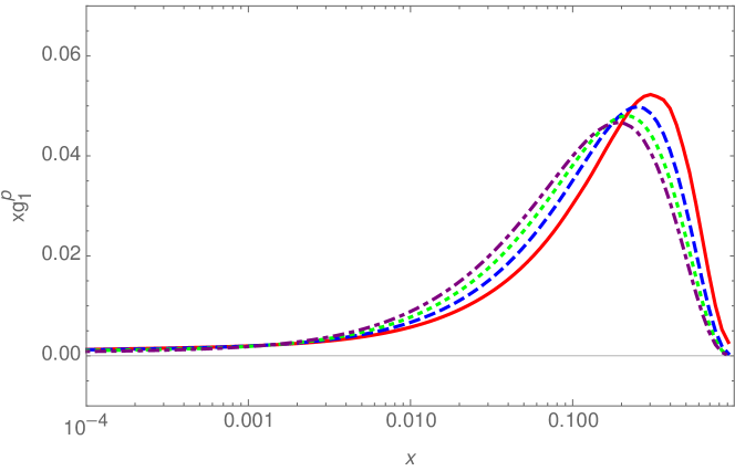
Figure 1: The NLO massless structure function $xg_{1}(x,Q^{2})$ as a function of $x$ for $Q^{2}=10\leavevmode\nobreak\ \rm GeV^{2}$ (full line); $100\leavevmode\nobreak\ \rm GeV^{2}$ (dashed line); $1000\leavevmode\nobreak\ \rm GeV^{2}$ (dotted line), and $10000\leavevmode\nobreak\ \rm GeV^{2}$ (dash–dotted line), using the parton distribution functions of [27].

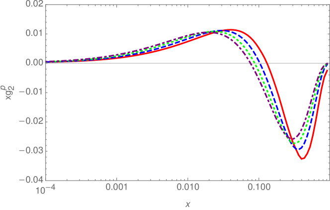
Figure 2: The NLO massless structure function $xg_{2}(x,Q^{2})$ as a function of $x$ for $Q^{2}=10\leavevmode\nobreak\ \rm GeV^{2}$ (full line); $100\leavevmode\nobreak\ \rm GeV^{2}$ (dashed line); $1000\leavevmode\nobreak\ \rm GeV^{2}$ (dotted line), and $10000\leavevmode\nobreak\ \rm GeV^{2}$ (dash–dotted line), using the parton distribution functions of [27].

The massless contributions to $xg_{1}^{p}(x,Q^{2})$ and $xg_{2}^{p}(x,Q^{2})$ are shown in Figures 1 and 2 to NLO. In all illustrations we use the parton distribution functions of Ref. [27] and $a_{s}(Q^{2})$ at NLO and they are made for contributions to the proton structure functions $xg_{1,(2)}^{p}(x,Q^{2})$.

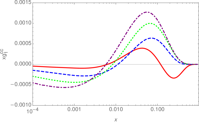
Figure 3: The $O(a_{s})$ charm contribution the polarized structure function $xg_{1}(x,Q^{2})$ as a function of $x$ for $Q^{2}=10\leavevmode\nobreak\ \rm GeV^{2}$ (full line); $100\leavevmode\nobreak\ \rm GeV^{2}$ (dashed line); $1000\leavevmode\nobreak\ \rm GeV^{2}$ (dotted line), and $10000\leavevmode\nobreak\ \rm GeV^{2}$ (dash–dotted line) for $m_{c}=1.59\leavevmode\nobreak\ \rm GeV$ and the parton distribution functions [27].

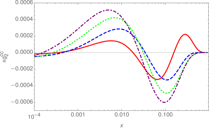
Figure 4: The $O(a_{s})$ charm contribution the polarized structure function $xg_{2}(x,Q^{2})$ as a function of $x$ for $Q^{2}=10\leavevmode\nobreak\ \rm GeV^{2}$ (full line); $100\leavevmode\nobreak\ \rm GeV^{2}$ (dashed line); $1000\leavevmode\nobreak\ \rm GeV^{2}$ (dotted line), and $10000\leavevmode\nobreak\ \rm GeV^{2}$ (dash–dotted line) for $m_{c}=1.59\leavevmode\nobreak\ \rm GeV$ and the parton distribution functions [27].

In the small $x$ region both structure functions tend to zero because of their principle shapes, which are similar to the unpolarized non–singlet structure functions. The change of sign in $xg_{2}(x,Q^{2})$ is due to the Wandzura–Wilczek relation. In Figure 3 we illustrate the charm contributions to the structure function $xg_{1}(x,Q^{2})$ at $O(a_{s})$ for $Q^{2}=10,100,1000$ and $10000\leavevmode\nobreak\ \rm GeV^{2}$.

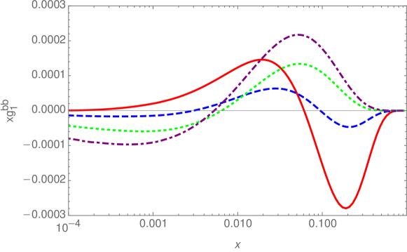
Figure 5: The $O(a_{s})$ bottom contribution the polarized structure function $xg_{1}(x,Q^{2})$ as a function of $x$ for $Q^{2}=10\leavevmode\nobreak\ \rm GeV^{2}$ (full line); $100\leavevmode\nobreak\ \rm GeV^{2}$ (dashed line); $1000\leavevmode\nobreak\ \rm GeV^{2}$ (dotted line), and $10000\leavevmode\nobreak\ \rm GeV^{2}$ (dash–dotted line) for $m_{b}=4.78\leavevmode\nobreak\ \rm GeV$ and the parton distribution functions [27].

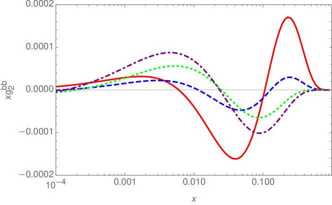
Figure 6: The $O(a_{s})$ bottom contribution the polarized structure function $xg_{2}(x,Q^{2})$ as a function of $x$ for $Q^{2}=10\leavevmode\nobreak\ \rm GeV^{2}$ (full line); $100\leavevmode\nobreak\ \rm GeV^{2}$ (dashed line); $1000\leavevmode\nobreak\ \rm GeV^{2}$ (dotted line), and $10000\leavevmode\nobreak\ \rm GeV^{2}$ (dash–dotted line) for $m_{b}=4.78\leavevmode\nobreak\ \rm GeV$ and the parton distribution functions [27].

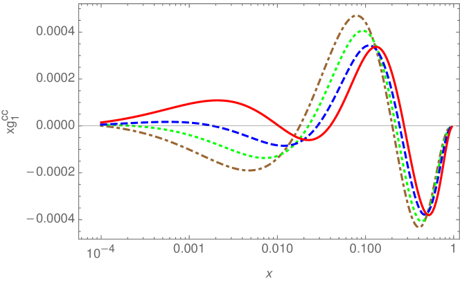
Figure 7: The $O(a_{s}^{2})$ charm contributions to the structure function $xg_{1}(x,Q^{2})$ for $m_{c}=1.59\leavevmode\nobreak\ \rm GeV$ as a function of $x$ for $Q^{2}=10\leavevmode\nobreak\ \rm GeV^{2}$ (full line); $100\leavevmode\nobreak\ \rm GeV^{2}$ (dashed line); $1000\leavevmode\nobreak\ \rm GeV^{2}$ (dotted line), and $10000\leavevmode\nobreak\ \rm GeV^{2}$ (dash–dotted line), using the parton distribution functions of [27].

The values of the charm and bottom quark masses are used in the on–shell scheme with $m_{c}=1.59\leavevmode\nobreak\ \rm GeV$, [107], and $m_{b}=4.78\leavevmode\nobreak\ \rm GeV$, [108].

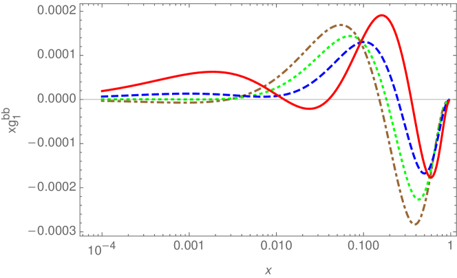
Figure 8: The $O(a_{s}^{2})$ bottom contributions to the structure function $xg_{1}(x,Q^{2})$ for $m_{b}=4.78\leavevmode\nobreak\ \rm GeV$ as a function of $x$ for $Q^{2}=10\leavevmode\nobreak\ \rm GeV^{2}$ (full line); $100\leavevmode\nobreak\ \rm GeV^{2}$ (dashed line); $1000\leavevmode\nobreak\ \rm GeV^{2}$ (dotted line), and $10000\leavevmode\nobreak\ \rm GeV^{2}$ (dash–dotted line), using the parton distribution functions of [27].

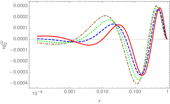
Figure 9: The $O(a_{s}^{2})$ charm contributions to the structure function $xg_{2}(x,Q^{2})$ for $m_{c}=1.59\leavevmode\nobreak\ \rm GeV$ as a function of $x$ for $Q^{2}=10\leavevmode\nobreak\ \rm GeV^{2}$ (full line); $100\leavevmode\nobreak\ \rm GeV^{2}$ (dashed line); $1000\leavevmode\nobreak\ \rm GeV^{2}$ (dotted line), and $10000\leavevmode\nobreak\ \rm GeV^{2}$ (dash–dotted line), using the parton distribution functions of [27].

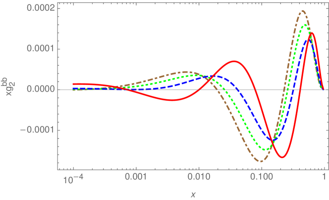
Figure 10: The $O(a_{s}^{2})$ bottom contributions to the structure function $xg_{2}(x,Q^{2})$ for $m_{b}=4.78\leavevmode\nobreak\ \rm GeV$ as a function of $x$ for $Q^{2}=10\leavevmode\nobreak\ \rm GeV^{2}$ (full line); $100\leavevmode\nobreak\ \rm GeV^{2}$ (dashed line); $1000\leavevmode\nobreak\ \rm GeV^{2}$ (dotted line), and $10000\leavevmode\nobreak\ \rm GeV^{2}$ (dash–dotted line), using the parton distribution functions of [27].

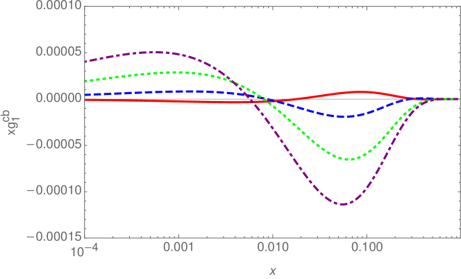
Figure 11: The $O(a_{s}^{2})$ two–mass contribution the polarized structure function $xg_{1}(x,Q^{2})$ as a function of $x$ for $Q^{2}=10\leavevmode\nobreak\ \rm GeV^{2}$ (full line); $100\leavevmode\nobreak\ \rm GeV^{2}$ (dashed line); $1000\leavevmode\nobreak\ \rm GeV^{2}$ (dotted line), and $10000\leavevmode\nobreak\ \rm GeV^{2}$ (dash–dotted line) for $m_{c}=1.59\leavevmode\nobreak\ \rm GeV$ and $m_{b}=4.78\leavevmode\nobreak\ \rm GeV$ and the parton distribution functions [27].

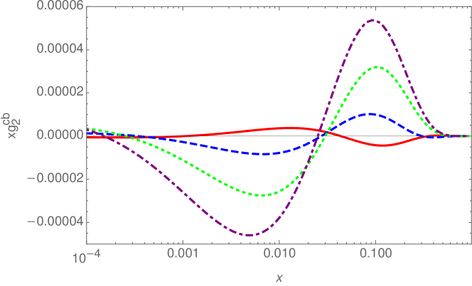
Figure 12: The $O(a_{s}^{2})$ two–mass contribution the polarized structure function $xg_{2}(x,Q^{2})$ as a function of $x$ for $Q^{2}=10\leavevmode\nobreak\ \rm GeV^{2}$ (full line); $100\leavevmode\nobreak\ \rm GeV^{2}$ (dashed line); $1000\leavevmode\nobreak\ \rm GeV^{2}$ (dotted line), and $10000\leavevmode\nobreak\ \rm GeV^{2}$ (dash–dotted line) for $m_{c}=1.59\leavevmode\nobreak\ \rm GeV$ and $m_{b}=4.78\leavevmode\nobreak\ \rm GeV$ and the parton distribution functions [27].

Figure 4 shows the corresponding contributions for the structure functions $xg_{2}(x,Q^{2})$. The numerical integrals have been performed using the Fortran code AIND [109]. The contributions to $xg_{1}$ turn out to be two to three times larger than to $xg_{2}$.

In Figures 5 and 6 the corresponding contributions due to bottom quarks are shown. They are suppressed by a factor of $\sim 8$ compared with the $O(a_{s})$ terms due to charm quarks. Comparing Figures 1 and 3, the $O(a_{s})$ charm contribution is suppressed by about one order of magnitude compared to the massless case for the structure function $xg_{1}(x,Q^{2})$ and similarly for the structure function $xg_{2}(x,Q^{2})$. Yet for future precision measurements, contributions of this kind become important.

We now turn to the single mass $O(a_{s}^{2})$ contributions. They are shown in Figures 7 and 9 for the charm contributions to $xg_{1(2)}(x,Q^{2})$ and for those from the bottom quark contributions to in Figures 8 and 10. Here we show the combination of the non–singlet and different singlet contributions. In the large $x$ region the non–singlet contribution dominates, while the singlet contributions dominate in the lower $x$ region. Towards large values of $x$ the Wandzura–Wilczek relation implies $g_{2}(x,Q^{2})\simeq-g_{1}(x,Q^{2})$. The bottom quark corrections turn out to be about a factor of 1.5 to 2 smaller than the charm quark contributions. The corrections of $O(a_{s}^{2})$ are a factor 2 to 3 smaller than the $O(a_{s})$ corrections in the case of charm, and similarly for bottom. Concerning the present illustrations, the corrections for bottom quarks can be trusted only in the higher $Q^{2}$ region. For the lower range of $Q^{2}$ one would need to consider also power corrections, which we did not do in the present analysis.

At $O(a_{s}^{2})$ there are also contributions with two heavy quark lines in single graphs, due to heavy quark polarization insertions in the external gluon line. Their contributions are illustrated in Figures 11 and 12. They are smaller in size by factors of 10–20 than the $O(a_{s})$ charm contributions.

6 The gluonic OMEs for the variable flavor number scheme

The matching between parton densities at large scales $Q^{2}\gg m^{2}$ can be performed by using the variable flavor number scheme, cf. e.g. [71]. Due to the similar size of $m_{c}$ and $m_{b}$ one often has to decouple both masses at the same time, see Eqs. (196–200) and (202, 203), cf. [65]. Besides the OMEs given in Section 4 already the polarized gluonic OMEs contribute which we calculate in the following. For the unrenormalized operator matrix element $\Delta A_{gq,Q}^{(2)}$ one obtains

$$\Delta A_{gq,Q}^{(2)} = S_{\varepsilon}^{2}\left(\frac{m^{2}}{\mu^{2}}\right)^{\varepsilon}(N+2)\biggl{\{}\frac{1}{\varepsilon^{2}}\frac{32}{3N(1+N)}+\frac{16}{\varepsilon}\biggl{[}\frac{(2+5N)}{9N(N+1)^{2}}-\frac{1}{3N(N+1)}S_{1}\biggr{]}$$ (178)

$$+\frac{8\big{(}22+41N+28N^{2}\big{)}}{27N(N+1)^{3}}-\frac{8(2+5N)}{9N(N+1)^{2}}S_{1}+\frac{4}{3N(N+1)}\left[S_{1}^{2}+S_{2}+2\zeta_{2}\right]$$

$$+\varepsilon\biggl{[}\frac{4\big{(}98+369N+408N^{2}+164N^{3}\big{)}}{81N(N+1)^{4}}-\biggl{(}\frac{4\big{(}22+41N+28N^{2}\big{)}}{27N(N+1)^{3}}+\frac{2}{3N(N+1)}S_{2}\biggr{)}$$

$$\times S_{1}+\frac{2(2+5N)}{9N(N+1)^{2}}S_{1}^{2}-\frac{2}{9N(N+1)}S_{1}^{3}+\frac{2(2+5N)}{9N(N+1)^{2}}S_{2}-\frac{4}{9N(N+1)}S_{3}$$

$$+\biggl{(}\frac{4(2+5N)}{9N(N+1)^{2}}-\frac{4}{3N(N+1)}S_{1}\biggr{)}\zeta_{2}+\frac{8}{9N(N+1)}\zeta_{3}\biggr{]}\biggr{\}}+O(\varepsilon^{2}).$$

The structure of $\Delta A_{gq,Q}^{(2),\rm L}$ is predicted, cf. [14], by

$$\Delta\hat{\hat{A}}_{gq,Q}^{(2),\rm L}=\left(\frac{m^{2}}{\mu^{2}}\right)^{\varepsilon}S_{\varepsilon}^{2}\left[-\frac{2\beta_{0,Q}}{\varepsilon^{2}}\Delta P_{gq}^{(0)}-\frac{1}{2\varepsilon}\Delta\hat{P}_{gq}^{(1)}+a_{gq,Q}^{(2)}+\varepsilon\overline{a}_{gq,Q}^{(2)}\right]+O(\varepsilon^{2}),$$ (179)

$$\Delta A_{gq,Q}^{(2),\rm L} = -\frac{\beta_{0,Q}}{2}\Delta P_{gq}^{(0)}\ln^{2}\left(\frac{m^{2}}{\mu^{2}}\right)-\frac{1}{2}\Delta\hat{P}_{gq}^{(1)}\ln\left(\frac{m^{2}}{\mu^{2}}\right)+a_{gq,Q}^{(2)}+\frac{\beta_{0,Q}\zeta_{2}}{2}\Delta P_{gq}^{(0)}.$$

$$= {\color[rgb]{0,0,0}C_{F}T_{F}}\Biggl{\{}\frac{8}{3}\frac{N+2}{N(N+1)}\ln^{2}\left(\frac{\mu^{2}}{m^{2}}\right)+16(N+2)\Biggl{[}\frac{S_{1}}{3N(N+1)}-\frac{(2+5N)}{9N(N+1)^{2}}\Biggr{]}\ln\left(\frac{\mu^{2}}{m^{2}}\right)$$

$$+(N+2)\Biggl{[}\frac{8\big{(}22+41N+28N^{2}\big{)}}{27N(N+1)^{3}}-\frac{8(2+5N)}{9N(N+1)^{2}}S_{1}+\frac{4}{3N(N+1)}\left[S_{1}^{2}+S_{2}\right]\Biggr{]}\Biggr{\}}.$$

The unrenormalized OMEs $\Delta\hat{\hat{A}}_{gg,Q}^{(1,(2)),\rm L}$ are given by

$$\Delta\hat{\hat{A}}_{gg,Q}^{(1)} ={} \left(\frac{m^{2}}{\mu^{2}}\right)^{\varepsilon/2}S_{\varepsilon}\left(-\frac{2\beta_{0,Q}}{\varepsilon}\right)\exp\left[\sum_{i=2}^{\infty}\frac{\zeta_{i}}{i}\left(\frac{\varepsilon}{2}\right)^{i}\right],$$ (182)

$$\Delta\hat{\hat{A}}_{gg,Q}^{(2),L} = \left(\frac{m^{2}}{\mu^{2}}\right)^{\varepsilon}S_{\varepsilon}^{2}\Biggl{\{}\frac{1}{\varepsilon^{2}}\Biggl{[}{\color[rgb]{0,0,0}C_{F}T_{F}}\frac{16(N-1)(2+N)}{N^{2}(1+N)^{2}}+{\color[rgb]{0,0,0}T_{F}^{2}}\frac{64}{9}+{\color[rgb]{0,0,0}C_{A}T_{F}}\Biggl{(}\frac{64}{3N(1+N)}$$ (183)

$$-\frac{32}{3}S_{1}\Biggr{)}\Biggr{]}+\frac{1}{\varepsilon}\Biggl{[}-{\color[rgb]{0,0,0}C_{F}T_{F}}\frac{4R_{2}}{N^{3}(1+N)^{3}}+{\color[rgb]{0,0,0}C_{A}T_{F}}\Biggl{(}+\frac{16R_{1}}{9N^{2}(1+N)^{2}}-\frac{80}{9}S_{1}\Biggr{)}\Biggr{]}$$

$$+{\color[rgb]{0,0,0}C_{F}T_{F}}\Biggl{(}-\frac{R_{5}}{3N^{4}(1+N)^{4}}+\frac{4(N-1)(2+N)\zeta_{2}}{N^{2}(1+N)^{2}}\Biggr{)}+{\color[rgb]{0,0,0}C_{A}T_{F}}\Biggl{(}\frac{2R_{3}}{27N^{3}(1+N)^{3}}$$

$$-\frac{4(47+56N)}{27(1+N)}S_{1}+\frac{16\zeta_{2}}{3N(1+N)}-\frac{8}{3}S_{1}\zeta_{2}\Biggr{)}+{\color[rgb]{0,0,0}T_{F}^{2}}\frac{16}{9}\zeta_{2}+\varepsilon\Biggl{[}{\color[rgb]{0,0,0}C_{F}T_{F}}\Biggl{(}-\frac{\zeta_{2}R_{7}}{N^{3}(1+N)^{3}}$$

$$-\frac{R_{6}}{12N^{5}(1+N)^{5}}+\frac{4(N-1)(2+N)\zeta_{3}}{3N^{2}(1+N)^{2}}\Biggr{)}+{\color[rgb]{0,0,0}C_{A}T_{F}}\Biggl{(}\frac{4\zeta_{2}R_{1}}{9N^{2}(1+N)^{2}}$$

$$+\frac{R_{4}}{81N^{4}(1+N)^{4}}-\frac{2\big{(}283+584N+328N^{2}\big{)}}{81(1+N)^{2}}S_{1}-\frac{S_{1}^{2}}{3(1+N)}+\frac{(1+2N)}{3(1+N)}S_{2}$$

$$-\frac{20}{9}\zeta_{2}S_{1}+\frac{16\zeta_{3}}{9N(1+N)}-\frac{8}{9}S_{1}\zeta_{3}\Biggr{)}+{\color[rgb]{0,0,0}T_{F}^{2}}\frac{8}{27}\zeta_{3}\Biggr{]},$$

with the polynomials

$$R_{1} = 3N^{4}+6N^{3}+16N^{2}+13N-3,$$ (184)

$$R_{2} = 3N^{6}+9N^{5}+7N^{4}+3N^{3}+8N^{2}-2N-4,$$ (185)

$$R_{3} = 15N^{6}+45N^{5}+374N^{4}+601N^{3}+161N^{2}-24N+36,$$ (186)

$$R_{4} = 3N^{8}+12N^{7}+2080N^{6}+5568N^{5}+4602N^{4}+1138N^{3}-3N^{2}-36N-108,$$ (187)

$$R_{5} = 13N^{8}+52N^{7}+54N^{6}+4N^{5}+13N^{4}+12N^{2}+36N+24,$$ (188)

$$R_{6} = 35N^{10}+175N^{9}+254N^{8}+62N^{7}+55N^{6}+347N^{5}+384N^{4}+72N^{3}-96N^{2}$$ (189)

$$-120N-48,$$

$$R_{7} = N^{6}+3N^{5}+5N^{4}+N^{3}-8N^{2}+2N+4.$$ (190)

In Eqs. (178, 183) we also present the terms of $O(\varepsilon)$ which are needed in the calculation of the NNLO contributions, cf. [14]. Furthermore, one has

$$\Delta\hat{\hat{A}}_{gg,Q}^{(2)} = \left(\frac{\hat{m}^{2}}{\mu^{2}}\right)^{\varepsilon}S_{\varepsilon}^{2}\Biggl{[}\frac{1}{2\varepsilon^{2}}\Biggl{\{}\Delta P_{gq}^{(0)}\Delta\hat{P}_{qg}^{(0)}+2\beta_{0,Q}\left(-\Delta P_{gg}^{(0)}+2\beta_{0}+4\beta_{0,Q}\right)\Biggr{\}}$$ (191)

$$+\frac{1}{2\varepsilon}\left[-\Delta\hat{P}^{(1)}_{gg}+4\delta m_{1}^{(-1)}\beta_{0,Q}\right]+a_{gg,Q}^{(2)}+2\delta m_{1}^{(0)}\beta_{0,Q}+\beta_{0,Q}^{2}\zeta_{2}$$

$$+\varepsilon\left[\overline{a}_{gg,Q}^{(2)}+2\delta m_{1}^{(1)}\beta_{0,Q}+\frac{1}{6}\beta_{0,Q}\zeta_{3}\right]\Biggr{]}.$$

The renormalized OME $\Delta A_{gg,Q}^{(2)}$ is then given by

$$\Delta A_{gg,Q}^{(1)} = -\beta_{0,Q}\ln\left(\frac{m^{2}}{\mu^{2}}\right),$$ (192)

$$\Delta A_{gg,Q}^{(2)} = \frac{1}{8}\left\{2\beta_{0,Q}\left(-\Delta P_{gg}^{(0)}+2\beta_{0}\right)+\Delta P_{gq}^{(0)}\Delta P_{qg}^{(0)}+8\beta_{0,Q}^{2}\right\}\ln^{2}\left(\frac{m^{2}}{\mu^{2}}\right)$$ (194)

$$-\frac{1}{2}\Delta\hat{P}_{gg}^{(1)}\ln\left(\frac{m^{2}}{\mu^{2}}\right)-\frac{\zeta_{2}}{8}\left[2\beta_{0,Q}\left(-\Delta P_{gg}^{(0)}+2\beta_{0}\right)+\Delta P_{gq}^{(0)}\Delta P_{qg}^{(0)}\right]+a_{gg,Q}^{(2)}$$

$$= \Biggl{[}{\color[rgb]{0,0,0}C_{F}T_{F}}\frac{4(N-1)(2+N)}{N^{2}(1+N)^{2}}+{\color[rgb]{0,0,0}T_{F}^{2}}\frac{16}{9}+{\color[rgb]{0,0,0}C_{A}T_{F}}\Biggl{(}\frac{16}{3N(1+N)}-\frac{8}{3}S_{1}\Biggr{)}\Biggr{]}\ln^{2}\left(\frac{\mu^{2}}{m^{2}}\right)$$

$$+\Biggl{[}-{\color[rgb]{0,0,0}C_{F}T_{F}}\frac{4R_{7}}{N^{3}(1+N)^{3}}+{\color[rgb]{0,0,0}C_{A}T_{F}}\Biggl{(}-\frac{16R_{1}}{9N^{2}(1+N)^{2}}+\frac{80}{9}S_{1}\Biggr{)}\Biggr{]}\ln\left(\frac{\mu^{2}}{m^{2}}\right)$$

$$+{\color[rgb]{0,0,0}C_{A}T_{F}}\Biggl{(}\frac{2R_{3}}{27N^{3}(1+N)^{3}}-\frac{4(47+56N)}{27(1+N)}S_{1}\Biggr{)}+{\color[rgb]{0,0,0}C_{F}T_{F}}\frac{R_{8}}{N^{4}(1+N)^{4}},$$

with

$$R_{8} = -15N^{8}-60N^{7}-82N^{6}-44N^{5}-15N^{4}-4N^{2}-12N-8.$$ (195)

The following transition rules hold in the two–flavor VFNS, cf. [71], to next–to–leading order in Mellin $N$ space

$$\Delta f_{{\sf NS},i}(N_{F}+2,\mu^{2}) = \Biggl{\{}1+a_{s}^{2}(\mu^{2})\left[\Delta A_{qq,Q}^{{\sf NS},(2,c)}+\Delta A_{qq,Q}^{{\sf NS},(2,b)}\right]\Biggr{\}}\Delta f_{{\sf NS},i}(N_{F},\mu^{2}),$$ (196)

$$\Delta\Sigma(N_{F}+2,\mu^{2}) = \Biggl{\{}1+a_{s}^{2}(\mu^{2})\Bigl{[}\Delta A_{qq,Q}^{{\sf NS},(2,c)}+\Delta A_{qq,Q}^{{\sf PS},(2,c)}+\Delta A_{qq,Q}^{{\sf NS},(2,b)}+\Delta A_{qq,Q}^{{\sf PS},(2,b)}\Bigr{]}\Biggr{\}}$$ (197)

$$\times\Delta\Sigma(N_{F},\mu^{2})$$

$$+\Biggl{\{}a_{s}(\mu^{2})\Bigl{[}\Delta A_{Qg}^{(1,c)}+\Delta A_{Qg}^{(1,b)}\Bigr{]}+a_{s}^{2}(\mu^{2})\Bigl{[}\Delta A_{Qg}^{(2,c)}+\Delta A_{Qg}^{(2,b)}+\Delta A_{Qg}^{(2,cb)}\Bigr{]}\Biggr{\}}$$

$$\times\Delta G(N_{F},\mu^{2}),$$

$$\Delta G(N_{F}+2,\mu^{2}) = \Biggl{\{}1+a_{s}(\mu^{2})\Bigl{[}\Delta A_{gg,Q}^{(1,c)}+\Delta A_{gg,Q}^{(1,b)}\Bigr{]}+a_{s}^{2}(\mu^{2})\Bigl{[}\Delta A_{gg,Q}^{(2,c)}+\Delta A_{gg,Q}^{(2,b)}$$

$$+\Delta A_{gg,Q}^{(2,cb)}\Bigr{]}\Biggr{\}}\Delta G(N_{F},\mu^{2})+a_{s}^{2}(\mu^{2})\Bigl{[}\Delta A_{gq,Q}^{(2,c)}+\Delta A_{gq,Q}^{(2,b)}\Bigr{]}\Delta\Sigma(N_{F},\mu^{2}),$$

$$\Bigl{[}\Delta f_{c}+\Delta f_{\bar{c}}\Bigr{]}(N_{F}+2,\mu^{2})=a_{s}^{2}(\mu^{2})\Delta A_{Qq}^{{\sf PS},(2,c)}\Delta\Sigma(N_{F},\mu^{2})+\Biggl{\{}a_{s}(\mu^{2})\Delta A_{Qg}^{(1,c)}$$ (199)

$$\leavevmode\nobreak\ \leavevmode\nobreak\ \leavevmode\nobreak\ \leavevmode\nobreak\ \leavevmode\nobreak\ \leavevmode\nobreak\ +a_{s}^{2}(\mu^{2})\Bigl{[}\Delta A_{Qg}^{(2,c)}+\frac{1}{2}\Delta A_{Qg}^{(2,cb)}\Bigr{]}\Biggr{\}}\Delta G(N_{F},\mu^{2}),$$

$$\Bigl{[}\Delta f_{b}+\Delta f_{\bar{b}}\Bigr{]}(N_{F}+2,\mu^{2})=a_{s}^{2}(\mu^{2})\Delta A_{Qq}^{{\sf PS},(2,b)}\Delta\Sigma(N_{F},\mu^{2})+\Biggl{\{}a_{s}(\mu^{2})\Delta A_{Qg}^{(1,b)}$$ (200)

$$\leavevmode\nobreak\ \leavevmode\nobreak\ \leavevmode\nobreak\ \leavevmode\nobreak\ \leavevmode\nobreak\ \leavevmode\nobreak\ +a_{s}^{2}(\mu^{2})\Bigl{[}\Delta A_{Qg}^{(2,b)}+\frac{1}{2}\Delta A_{Qg}^{(2,cb)}\Bigr{]}\Biggr{\}}\Delta G(N_{F},\mu^{2}),$$

and

$$\Delta f_{{\sf NS},i}(N_{F},\mu^{2}) = \Delta q_{i}(\mu^{2})+\Delta\bar{q}_{i}(\mu^{2}).$$ (201)

The two–mass OMEs read

$$\Delta A_{Qg}^{(2,cb)} = -\beta_{0,Q}\Delta\hat{\gamma}_{qg}^{(0)}\ln\left(\frac{\mu^{2}}{m_{c}^{2}}\right)\ln\left(\frac{\mu^{2}}{m_{b}^{2}}\right),$$ (202)

$$\Delta A_{gg,Q}^{(2,cb)} = 2\beta_{0,Q}^{2}\ln\left(\frac{\mu^{2}}{m_{c}^{2}}\right)\ln\left(\frac{\mu^{2}}{m_{b}^{2}}\right).$$ (203)

Very recently the three–loop corrections to $\Delta A_{gg,Q}^{(3)}$ have been completed [111].

7 Conclusions

We calculated the two–loop single and double mass corrections to the polarized twist–2 structure function $g_{1}(x,Q^{2})$ in the asymptotic range $Q^{2}\gg m^{2}$ in analytic form. Those to $g_{2}(x,Q^{2})$ are related by the Wandzura–Wilczek relation. The corrections include all but the power contributions $\propto(m^{2}/Q^{2})^{k},\leavevmode\nobreak\ k\in\mathbb{N},k\geq 1$. Parts of the results in Ref. [1] were confirmed, and other parts were corrected. In [1] a series of contributions to the Wilson coefficients of the structure function $g_{1}(x,Q^{2})$, like additional terms contributing to the non–singlet Wilson coefficient, $\Delta H_{g}^{(2)}$, and $\Delta L_{g}^{(2)}$, were left out. Also the two–mass corrections were not considered there. We perform the calculation of the Feynman diagrams using the hypergeometric method [59] for general values of the dimensional parameter $\varepsilon$ in the Larin scheme and transform then to the M scheme and do not use IBP reduction. In Mellin space one obtains more compact results than in momentum fraction space. In Ref. [1], 24 Nielsen integrals [112] were needed, whereas the $N$–space result depends only on two functions using also structural relations [93]. In the small $x$ region the heavy flavor contributions are suppressed by at least one power of $\ln(x)$ if compared to the expected leading logarithmic behaviour of $O((a_{s}\ln^{2}(x))^{k})$ in the massless case. We illustrated the different contributions to two–loop order for the structure functions $xg_{1}(x,Q^{2})$ and $xg_{2}(x,Q^{2})$ in a wide kinematic range for planning future experiments and possible re–analysis of the existing data.

The contributions calculated in the present paper are of importance for precision measurements of the structure functions $g_{1}(x,Q^{2})$ and $g_{2}(x,Q^{2})$ in future high luminosity measurements, e.g. at the EIC [7], and associated precision measurements of the strong coupling constant $a_{s}$ [113] and the charm quark mass [107]. We also presented the polarized NLO expansion coefficients in the 2–heavy flavor variable flavor number scheme and the next order terms $O(\varepsilon)$ needed in the calculation of the $O(a_{s}^{3})$ massive OMEs.

Appendix A Results for the Individual Diagrams

In this appendix we list the results for the individual diagrams to $O(\varepsilon)$, prior to renormalization. The calculation was performed in Feynman gauge. We suppress the argument in $S_{\vec{a}}(N)\equiv S_{\vec{a}}$ and the factor

$$ia_{s}^{2}S_{\varepsilon}^{2}\Biggl{(}\frac{m^{2}}{\mu^{2}}\Biggr{)}^{\varepsilon/2}\frac{1-(-1)^{N}}{2}.$$

The notation follows Ref. [11], where also the individual diagrams are depicted.

$$\Delta A^{Qg}_{a} = T_{F}C_{F}\Biggl{\{}\frac{1}{\varepsilon^{2}}\Biggl{[}\frac{-16(N-1)}{N^{2}(N+1)^{2}}\Biggr{]}+\frac{1}{\varepsilon}\Biggl{[}8\frac{(N-1)(2N+1)}{N^{3}(N+1)^{3}}\Biggr{]}-\frac{4(N-1)}{N^{2}(N+1)^{2}}\Bigl{(}2S_{2}+\zeta_{2}\Bigr{)}$$ (204)

$$+\frac{4\hat{P}_{1}}{N^{4}(N+1)^{4}}+\varepsilon\Biggl{[}\frac{-4(N-1)}{3N^{2}(N+1)^{2}}\Bigl{(}3S_{3}+\zeta_{3}\Bigr{)}+2\frac{(N-1)(2N+1)}{N^{3}(N+1)^{3}}\Bigl{(}2S_{2}+\zeta_{2}\Bigr{)}$$

$$-\frac{2\hat{P}_{2}}{N^{5}(N+1)^{5}}\Biggr{]}\Biggr{\}}\leavevmode\nobreak\ ,$$

$$\hat{P}_{1} = (N-1)(3N^{4}+2N^{3}-2N^{2}+N+1)\leavevmode\nobreak\ ,$$ (205)

$$\hat{P}_{2} = 2N^{7}+10N^{6}+21N^{5}+7N^{4}-7N^{3}-3N^{2}+N+1\leavevmode\nobreak\ .$$ (206)

$$\Delta A^{Qg}_{b} = T_{F}C_{F}\Biggl{\{}\frac{1}{\varepsilon^{2}}\Biggl{[}\frac{32(N-1)}{N(N+1)}\Bigl{(}S_{1}-1\Bigr{)}\Biggr{]}+\frac{1}{\varepsilon}\Biggl{[}\frac{8(N-1)}{N(N+1)}\Bigl{(}S_{1}^{2}-3S_{2}\Bigr{)}-\frac{16(N^{2}+1)}{N(N+1)^{2}}S_{1}$$ (207)

$$+\frac{32N}{(N+1)^{2}}\Biggr{]}+\frac{4(N-1)}{3N(N+1)}\Bigl{(}12S_{2,1}-10S_{3}+3S_{1}S_{2}+S_{1}^{3}+6S_{1}\zeta_{2}-6\zeta_{2}\Bigr{)}$$

$$-\frac{4(N^{2}-7)}{N(N+1)^{2}}S_{2}-\frac{4(N^{2}+1)}{N(N+1)^{2}}S_{1}^{2}+16\frac{N^{4}+2N^{3}+N^{2}-2N+1}{N^{2}(N+1)^{3}}S_{1}$$

$$-16\frac{2N^{3}+2N^{2}+1}{N(N+1)^{3}}$$

$$+\varepsilon\Biggl{[}\frac{N-1}{N(N+1)}\Bigl{(}-8S_{2,1,1}+8S_{3,1}-11S_{4}+8S_{2,1}S_{1}+\frac{4}{3}S_{3}S_{1}-\frac{7}{2}S_{2}^{2}+S_{2}S_{1}^{2}+\frac{1}{6}S_{1}^{4}$$

$$-\frac{8}{3}\zeta_{3}-6\zeta_{2}S_{2}+2\zeta_{2}S_{1}^{2}+\frac{8}{3}S_{1}\zeta_{3}\Bigr{)}+\frac{N^{2}+1}{N(N+1)^{2}}\Bigl{(}-8S_{2,1}-2S_{2}S_{1}-\frac{2}{3}S_{1}^{3}-4S_{1}\zeta_{2}\Bigr{)}$$

$$-\frac{4}{3}\frac{N^{2}-11}{N(N+1)^{2}}S_{3}+4\frac{N^{4}+2N^{3}+N^{2}+2N+1}{N^{2}(N+1)^{3}}S_{2}+\frac{8N\zeta_{2}}{(N+1)^{2}}-\frac{8\hat{P}_{3}S_{1}}{N^{2}(N+1)^{4}}$$

$$+4\frac{N^{4}+2N^{3}+N^{2}-2N+1}{N^{2}(N+1)^{3}}S_{1}^{2}+8\frac{4N^{4}+8N^{3}+4N^{2}+2N+3}{N(N+1)^{4}}\Biggr{]}\Biggr{\}}\leavevmode\nobreak\ ,$$

$$\hat{P}_{3} = 2N^{5}+6N^{4}+6N^{3}+3N^{2}+8N+2\leavevmode\nobreak\ .$$ (208)

$$\Delta A^{Qg}_{c} = T_{F}C_{F}\Biggl{\{}\frac{1}{\varepsilon^{2}}\Biggl{[}\frac{8(N-1)}{N(N+1)}\Biggr{]}+\frac{1}{\varepsilon}\Biggl{[}-4\frac{13N^{4}+14N^{3}+2N^{2}+5N+2}{N^{2}(N+1)^{2}(N+2)}\Biggr{]}$$

$$-\frac{2(N-1)}{N(N+1)}\Bigl{(}10S_{2}-\zeta_{2}\Bigr{)}+\frac{2\hat{P}_{4}}{N^{3}(N+1)^{3}(N+2)}+\varepsilon\Biggl{[}-\frac{2(N-1)}{3N(N+1)}\Bigl{(}15S_{3}-\zeta_{3}\Bigr{)}$$

$$-\frac{13N^{4}+14N^{3}+2N^{2}+5N+2}{N^{2}(N+1)^{2}(N+2)}\zeta_{2}+2\frac{7N^{3}-10N-1}{N^{2}(N+1)^{2}}S_{2}-\frac{\hat{P}_{5}}{N^{4}(N+1)^{4}(N+2)}\Biggr{]}\Biggr{\}}\leavevmode\nobreak\ ,$$

$$\hat{P}_{4} = 16N^{6}+32N^{5}-4N^{4}-44N^{3}-11N^{2}-7N-2\leavevmode\nobreak\ ,$$ (210)

$$\hat{P}_{5} = 32N^{8}+96N^{7}+65N^{6}-45N^{5}-24N^{4}+19N^{3}+18N^{2}+9N+2\leavevmode\nobreak\ .$$ (211)

$$\Delta A^{Qg}_{d} = T_{F}C_{F}\Biggl{\{}\frac{1}{\varepsilon^{2}}\Biggl{[}\frac{16(N-1)}{N(N+1)}\Biggr{]}+\frac{1}{\varepsilon}\Biggl{[}\frac{8(N-1)}{N(N+1)}S_{1}-8\frac{N^{3}+8N^{2}-5N-10}{N(N+1)^{2}(N+2)}\Biggr{]}$$ (212)

$$+\frac{2(N-1)}{N(N+1)}\Bigl{(}S_{2}+S_{1}^{2}+2\zeta_{2}\Bigr{)}-4\frac{N^{3}+6N^{2}-11N+2}{N^{2}(N+1)^{2}}S_{1}+8\frac{N^{4}+7N^{3}-9N+6}{N(N+1)^{3}(N+2)}$$

$$+\varepsilon\Biggl{[}\frac{1}{3}\frac{N-1}{N(N+1)}\Bigl{(}12S_{2,1}+2S_{3}+3S_{2}S_{1}+S_{1}^{3}+4\zeta_{3}+6\zeta_{2}S_{1}\Bigr{)}$$

$$-\frac{N^{3}+6N^{2}-11N+2}{N^{2}(N+1)^{2}}\Bigl{(}S_{2}+S_{1}^{2}\Bigr{)}-2\frac{N^{3}+8N^{2}-5N-10}{N(N+1)^{2}(N+2)}\zeta_{2}$$

$$+4\frac{N^{4}+6N^{3}-5N^{2}-2N+1}{N^{2}(N+1)^{3}}S_{1}-\frac{4\hat{P}_{6}}{N(N+1)^{4}(N+2)}\Biggr{]}\Biggr{\}}\leavevmode\nobreak\ ,$$

$$\hat{P}_{6} = 2N^{5}+16N^{4}+14N^{3}-21N^{2}-22N-8\leavevmode\nobreak\ .$$ (213)

$$\Delta A^{Qg}_{e} = T_{F}\Bigl{(}C_{F}-\frac{C_{A}}{2}\Bigr{)}\Biggl{\{}\frac{1}{\varepsilon^{2}}\Biggl{[}\frac{-16(N-1)}{N(N+1)}\Biggr{]}+\frac{1}{\varepsilon}\Biggl{[}\frac{8S_{1}}{N}+\frac{8(N-1)}{N^{2}(N+1)^{2}}\Biggr{]}+\frac{2(N-2)}{N(N+2)}S_{1}^{2}$$ (214)

$$+2\frac{9N^{2}+7N-10}{N(N+1)(N+2)}S_{2}-4\frac{4N^{4}+7N^{3}+9N^{2}+14N-8}{N^{2}(N+1)^{2}(N+2)}S_{1}-\frac{4\hat{P}_{7}}{N^{3}(N+1)^{3}(N+2)}$$

$$-\frac{4(N-1)}{N(1+N)}\zeta_{2}+\varepsilon\Biggl{[}2\frac{2S_{2,1}+S_{1}\zeta_{2}}{N}+\frac{N-2}{3N(N+2)}\Bigl{(}3S_{2}S_{1}+S_{1}^{3}\Bigr{)}-\frac{4}{3}\frac{N-1}{N(N+1)}\zeta_{3}$$

$$+\frac{2}{3}\frac{13N^{2}+11N-14}{N(N+1)(N+2)}S_{3}-\frac{20N^{3}+39N^{2}+13N+2}{N(N+1)^{2}(N+2)}S_{2}+\frac{2\hat{P}_{8}S_{1}}{N^{2}(N+1)^{3}(N+2)}$$

$$-\frac{4N^{4}+3N^{3}+5N^{2}+14N-8}{N^{2}(N+1)^{2}(N+2)}S_{1}^{2}+\frac{2(N-1)}{N^{2}(N+1)^{2}}\zeta_{2}+\frac{2\hat{P}_{9}}{N^{4}(N+1)^{4}(N+2)}\Biggr{]}\Biggr{\}}\leavevmode\nobreak\ ,$$

$$\hat{P}_{7} = 2N^{5}-13N^{4}-28N^{3}+4N^{2}+N+2\leavevmode\nobreak\ ,$$ (215)

$$\hat{P}_{8} = 8N^{5}+22N^{4}+35N^{3}+35N^{2}-18N-16\leavevmode\nobreak\ ,$$ (216)

$$\hat{P}_{9} = 8N^{7}-4N^{6}-26N^{5}+34N^{4}+38N^{3}+3N^{2}-3N-2\leavevmode\nobreak\ .$$ (217)

$$\Delta A^{Qg}_{f} = T_{F}\Bigl{(}C_{F}-\frac{C_{A}}{2}\Bigr{)}\Biggl{\{}\frac{1}{\varepsilon}\Biggl{[}\frac{16(N-1)}{N(N+1)}S_{2}-16\frac{(2N+1)(N-1)}{N^{2}(N+1)^{2}}S_{1}\Biggr{]}-\frac{8(N-1)}{N(N+1)}\Bigl{(}2S_{2,1}-S_{3}\Bigr{)}$$

$$-4\frac{(2N+3)(7N+1)}{N^{2}(N+1)^{2}}S_{2}-4\frac{(2N+1)(N-1)}{N^{2}(N+1)^{2}}S_{1}^{2}+8\frac{2N^{3}+11N^{2}+21N+6}{N^{2}(N+1)^{3}}S_{1}$$

$$+\varepsilon\Biggl{[}\frac{4(N-1)}{N(N+1)}\Bigl{(}-2S_{2,1,1}+2S_{4}+S_{2}^{2}+S_{2}\zeta_{2}\Bigr{)}+\frac{8(3N+1)}{N^{2}(N+1)^{2}}S_{2,1}-\frac{20}{3}\frac{4N^{2}+7N+1}{N^{2}(N+1)^{2}}S_{3}$$

$$+2\frac{(2N+1)(N-1)}{3N^{2}(N+1)^{2}}\Bigl{(}-3S_{2}S_{1}-S_{1}^{3}-6S_{1}\zeta_{2}\Bigr{)}-2\frac{10N^{3}+17N^{2}+11N+2}{N^{2}(N+1)^{3}}S_{2}$$ (218)

$$+2\frac{2N^{3}+11N^{2}+21N+6}{N^{2}(N+1)^{3}}S_{1}^{2}-4\frac{4N^{4}+4N^{3}-13N^{2}-33N-10}{N^{2}(N+1)^{4}}S_{1}\Biggr{]}\Biggr{\}}\leavevmode\nobreak\ .$$

$$\Delta A^{Qg}_{j} = T_{F}C_{A}\Biggl{\{}\frac{1}{\varepsilon^{2}}\Biggl{[}16\frac{(N+4)(N-1)}{N^{2}(N+1)^{2}}\Biggr{]}+\frac{1}{\varepsilon}\Biggl{[}-8\frac{(N+4)(N^{3}+2N+1)}{N^{3}(N+1)^{3}}\Biggr{]}$$ (219)

$$+4\frac{(N+4)(N-1)}{N^{2}(N+1)^{2}}\Bigl{(}2S_{2}+\zeta_{2}\Bigr{)}+4\frac{(N+4)(4N^{3}-4N^{2}-3N-1)}{(N+1)^{4}N^{4}}$$

$$+\varepsilon\Biggl{[}-\frac{2\hat{P}_{10}}{N^{5}(N+1)^{5}}+4\frac{(N+4)(N-1)}{3N^{2}(N+1)^{2}}\Bigl{(}3S_{3}+\zeta_{3}\Bigr{)}$$

$$-2\frac{(N+4)(N^{3}+2N+1)}{N^{3}(N+1)^{3}}\Bigl{(}2S_{2}+\zeta_{2}\Bigr{)}\Biggr{]}\Biggr{\}}\leavevmode\nobreak\ ,$$

$$\hat{P}_{10} = (N+4)(N^{5}-7N^{4}+6N^{3}+7N^{2}+4N+1)\leavevmode\nobreak\ .$$ (220)

$$\Delta A^{Qg}_{l} = T_{F}C_{A}\Biggl{\{}\frac{1}{\varepsilon^{2}}\Biggl{[}-\frac{8(2N-1)}{N(N+1)}S_{1}-16\frac{N^{3}+N^{2}-2N-1}{(N+1)^{2}N^{2}}\Biggr{]}+\frac{1}{\varepsilon}\Biggl{[}\frac{-2(2N-1)}{N(N+1)}\Bigl{(}S_{2}+S_{1}^{2}\Bigr{)}$$ (221)

$$+\frac{12S_{1}}{N(N+1)^{2}}+\frac{8\hat{P}_{11}}{N^{3}(N+1)^{3}}\Biggr{]}-\frac{2N-1}{3N(N+1)}\Bigl{(}12S_{2,1}+2S_{3}+3S_{2}S_{1}+S_{1}^{3}+6S_{1}\zeta_{2}\Bigr{)}$$

$$+\frac{3S_{1}^{2}}{N(N+1)^{2}}+2\frac{7N^{3}-2N^{2}+4N+4}{N^{2}(N+1)^{3}}S_{1}+\frac{8N^{3}-N+8}{N^{2}(N+1)^{2}}S_{2}$$

$$-4\frac{N^{3}+N^{2}-2N-1}{N^{2}(N+1)^{2}}\zeta_{2}-\frac{4\hat{P}_{12}}{N^{4}(N+1)^{4}}+\varepsilon\Biggl{[}\frac{2N-1}{N(N+1)}\Bigl{(}2S_{2,1,1}-2S_{3,1}-\frac{5}{4}S_{4}$$

$$-2S_{2,1}S_{1}-\frac{1}{3}S_{3}S_{1}-\frac{9}{8}S_{2}^{2}-\frac{1}{4}S_{2}S_{1}^{2}-\frac{1}{24}S_{1}^{4}-\frac{1}{2}S_{2}\zeta_{2}-\frac{1}{2}S_{1}^{2}\zeta_{2}-\frac{2}{3}S_{1}\zeta_{3}\Bigr{)}$$

$$+\frac{12S_{2,1}+3S_{2}S_{1}+S_{1}^{3}+6\zeta_{2}S_{1}}{2N(N+1)^{2}}-\frac{\hat{P}_{13}S_{2}}{2N^{3}(N+1)^{3}}$$

$$+\frac{7N^{3}-2N^{2}+4N+4}{2N^{2}(N+1)^{3}}S_{1}^{2}-\frac{14N^{4}+13N^{3}+12N^{2}+6N+8}{N^{2}(N+1)^{4}}S_{1}+\frac{2\hat{P}_{14}\zeta_{2}}{N^{3}(N+1)^{3}}$$

$$-\frac{4}{3}\frac{N^{3}+N^{2}-2N-1}{N^{2}(N+1)^{2}}\zeta_{3}+\frac{4N^{3}-N+4}{N^{2}(N+1)^{2}}S_{3}+\frac{2\hat{P}_{15}}{N^{5}(N+1)^{5}}\Biggr{]}\Biggr{\}}\leavevmode\nobreak\ ,$$

$$\hat{P}_{11} = (2N+1)(N^{4}+N^{3}+2N+1)\leavevmode\nobreak\ ,$$ (222)

$$\hat{P}_{12} = 4N^{7}+12N^{6}+5N^{5}+4N^{4}-2N^{3}-10N^{2}-5N-1\leavevmode\nobreak\ ,$$ (223)

$$\hat{P}_{13} = 16N^{5}+21N^{4}+2N^{3}-36N^{2}-36N-8\leavevmode\nobreak\ ,$$ (224)

$$\hat{P}_{14} = (2N+1)(N^{4}+N^{3}+2N+1)\leavevmode\nobreak\ ,$$ (225)

$$\hat{P}_{15} = (2N+1)(4N^{8}+14N^{7}+9N^{6}+N^{5}-N^{4}+6N^{3}+7N^{2}+4N+1)\leavevmode\nobreak\ .$$ (226)

$$\Delta A^{Qg}_{m} = T_{F}C_{A}\Biggl{\{}\frac{1}{\varepsilon^{2}}\Biggl{[}-\frac{16(N-1)}{N^{2}(N+1)^{2}}\Biggr{]}+\frac{1}{\varepsilon}\Biggl{[}4\frac{N^{4}+7N^{3}+3N^{2}+3N+2}{N^{3}(N+1)^{3}}\Biggr{]}$$

$$-\frac{4(N-1)}{N^{2}(N+1)^{2}}\Bigl{(}2S_{2}+\zeta_{2}\Bigr{)}-\frac{2\hat{P}_{16}}{N^{4}(N+1)^{4}}+\varepsilon\Biggl{[}\frac{-4(N-1)}{3N^{2}(N+1)^{2}}\Bigl{(}3S_{3}+\zeta_{3}\Bigr{)}$$ (227)

$$+\frac{N^{4}+7N^{3}+3N^{2}+3N+2}{N^{3}(N+1)^{3}}\Bigl{(}2S_{2}+\zeta_{2}\Bigr{)}-\frac{\hat{P}_{17}}{N^{5}(N+1)^{5}}\Biggr{]}\Biggr{\}}\leavevmode\nobreak\ ,$$

$$\hat{P}_{16} = 6N^{5}+5N^{4}+N^{3}-13N^{2}-5N-2\leavevmode\nobreak\ ,$$ (228)

$$\hat{P}_{17} = 3N^{6}-10N^{5}-9N^{4}-29N^{3}-18N^{2}-7N-2\leavevmode\nobreak\ .$$ (229)

$$\Delta A^{Qg}_{n} = T_{F}C_{A}\Biggl{\{}\frac{1}{\varepsilon^{2}}\Biggl{[}-\frac{8(2N-3)}{N(N+1)}S_{1}+8\frac{N^{3}+N-4}{N^{2}(N+1)^{2}}\Biggr{]}+\frac{1}{\varepsilon}\Biggl{[}-\frac{16(N-1)}{N(N+1)}S_{-2}+\frac{2(2N-1)}{N(N+1)}S_{2}$$ (230)

$$-\frac{2(2N-3)}{N(N+1)}S_{1}^{2}+4\frac{N^{3}-2N^{2}+8N+2}{N^{2}(N+1)^{2}}S_{1}-4\frac{2N^{4}+3N^{3}+8N^{2}+N+8}{N^{2}(N+1)^{3}}\Biggr{]}$$

$$+\frac{8(N-1)}{N(N+1)}\Bigl{(}2S_{-2,1}-S_{-3}-2S_{-2}S_{1}\Bigr{)}+\frac{4S_{2,1}}{N(N+1)}-\frac{2N-3}{3N(N+1)}\Bigl{(}S_{1}^{3}+6S_{1}\zeta_{2}\Bigr{)}$$

$$-\frac{2(8N-9)}{3N(N+1)}S_{3}-\frac{10N-11}{N(N+1)}S_{2}S_{1}-\frac{16(N-1)}{N(N+1)^{2}}S_{-2}+\frac{N^{3}-10N^{2}-20N-22}{N^{2}(N+1)^{2}}S_{2}$$

$$+\frac{N^{3}-2N^{2}+8N+2}{N^{2}(N+1)^{2}}S_{1}^{2}+2\frac{N^{3}+N-4}{N^{2}(N+1)^{2}}\zeta_{2}-2\frac{2N^{4}+2N^{3}-4N^{2}-35N-12}{N^{2}(N+1)^{3}}S_{1}$$

$$+\frac{2\hat{P}_{18}}{N^{2}(N+1)^{4}}+\varepsilon\Biggl{[}\frac{4(N-1)}{N(N+1)}\Bigl{(}-4S_{-2,1,1}+2S_{-3,1}+2S_{-2,2}-S_{-4}+4S_{-2,1}S_{1}$$

$$-2S_{-3}S_{1}-2S_{-2}S_{2}-2S_{-2}S_{1}^{2}-S_{-2}\zeta_{2}\Bigr{)}+\frac{8(N-1)}{N(N+1)^{2}}\Bigl{(}2S_{-2,1}-S_{-3}-2S_{-2}S_{1}\Bigr{)}$$

$$+\frac{2(4N-3)}{N(N+1)}S_{3,1}-\frac{2N-1}{2N(N+1)}\Bigl{(}4S_{2,1,1}-4S_{2,1}S_{1}-S_{2}\zeta_{2}\Bigr{)}-\frac{2N-3}{24N(N+1)}\Bigl{(}30S_{4}$$

$$+S_{1}^{4}+12S_{1}^{2}\zeta_{2}+16S_{1}\zeta_{3}\Bigr{)}$$

$$-\frac{38N-39}{3N(N+1)}S_{3}S_{1}+\frac{3(10N-7)}{8N(N+1)}S_{2}^{2}-\frac{18N-19}{4N(N+1)}S_{2}S_{1}^{2}+2\frac{N^{3}+2N^{2}+4N+2}{N^{2}(N+1)^{2}}S_{2,1}$$

$$+\frac{N^{3}-38N^{2}-10N-34}{3N^{2}(N+1)^{2}}S_{3}+\frac{N^{3}-2N^{2}+8N+2}{6N^{2}(N+1)^{2}}S_{1}^{3}+\frac{N^{3}-18N^{2}+24N+2}{2N^{2}(N+1)^{2}}S_{2}S_{1}$$

$$+\frac{N^{3}-2N^{2}+8N+2}{N^{2}(N+1)^{2}}S_{1}\zeta_{2}+\frac{2}{3}\frac{N^{3}+N-4}{N^{2}(N+1)^{2}}\zeta_{3}+\frac{8(N^{2}+3)}{N(N+1)^{3}}S_{-2}$$

$$-\frac{2N^{4}-18N^{3}-20N^{2}-3N+36}{2N^{2}(N+1)^{3}}S_{2}-\frac{2N^{4}+2N^{3}-4N^{2}-35N-12}{2N^{2}(N+1)^{3}}S_{1}^{2}$$

$$-\frac{2N^{4}+3N^{3}+8N^{2}+N+8}{N^{2}(N+1)^{3}}\zeta_{2}+\frac{\hat{P}_{19}}{N^{2}(N+1)^{4}}S_{1}-\frac{\hat{P}_{20}}{N^{2}(N+1)^{5}}\Biggr{]}\Biggr{\}}\leavevmode\nobreak\ ,$$

$$\hat{P}_{18} = 4N^{5}+10N^{4}+11N^{3}-16N^{2}-19N-24\leavevmode\nobreak\ ,$$ (231)

$$\hat{P}_{19} = 4N^{5}+8N^{4}-10N^{2}+51N+20\leavevmode\nobreak\ ,$$ (232)

$$\hat{P}_{20} = 8N^{6}+28N^{5}+42N^{4}+19N^{3}+24N^{2}+13N+40\leavevmode\nobreak\ .$$ (233)

Furthermore, one has

$$\Delta A^{Qg}_{g} = \Delta A^{Qg}_{h}=\Delta A^{Qg}_{i}=\Delta A^{Qg}_{k}=\Delta A^{Qg}_{o}=\Delta A^{Qg}_{p}=\Delta A^{Qg}_{q}=\Delta A^{Qg}_{r}=\Delta A^{Qg}_{r^{\prime}}$$ (234)

$$= \Delta A^{Qg}_{s}=\Delta A^{Qg}_{t}=0\leavevmode\nobreak\ .$$

In Table 3 we show, for comparison, numerical values for some moments of the diagrams calculated above.

The non–singlet diagrams are the same as in the unpolarized case, cf. [11, 16]. These sums were calculated both with the help of integral representations and by applying the package Sigma, [114, 115].

Table 3: Numerical moments for $N=3,7$ for the different contributions in the dimensional parameter $\varepsilon$ to the diagrams $A-N$ of Ref. [1].

Appendix B Representations through generalized hypergeometric series

In the present calculation the Feynman diagrams were evaluated without using the integration-by-parts method. As an example, we describe in the following the evaluation of a $5$–propagator integral emerging in diagram $f$, see Figure 3, Ref. [11].

$$I_{f}(N) = \sum_{i=0}^{N-2}\int_{0}^{1}\!\int_{0}^{1}\!\frac{d^{D}q\leavevmode\nobreak\ d^{D}k}{(2\pi)^{D}(2\pi)^{D}}\frac{(\Delta q)^{i}(\Delta k)^{N-2-i}}{(\!q^{2}-\!m^{2})((\!q-\!p)^{2}-\!m^{2})(\!k^{2}-\!m^{2})((\!k-\!p)^{2}-\!m^{2})^{2}(\!k-\!q)^{2}}\leavevmode\nobreak\ .$$

The diagram has a 4–dimensional Feynman parameterization over the generalized unit-cube. After the momentum integrals are carried out one obtains

$$I_{f}(N) = \frac{(\Delta p)^{N-2}\Gamma(1-\varepsilon)}{(4\pi)^{4+\varepsilon}(m^{2})^{1-\varepsilon}}\int_{0}^{1}\int_{0}^{1}\!\int_{0}^{1}\!\int_{0}^{1}\!dudzdydx\frac{(1-u)^{-\varepsilon/2}z^{-\varepsilon/2}(1-z)^{\varepsilon/2-1}}{(1-u+uz)^{1-\varepsilon}(x-y)}$$ (236)

$$\Biggl{[}\Bigl{(}zyu+x(1-zu)\Bigr{)}^{N-1}-\Bigl{(}(1-u)x+uy\Bigr{)}^{N-1}\Biggr{]}\leavevmode\nobreak\ .$$

It is very useful to apply the following transformations of variables given in Ref. [116],

$$x^{\prime} := xy\leavevmode\nobreak\ ,\quad\hskip 46.94704pty^{\prime}:=\frac{x(1-y)}{1-xy}\leavevmode\nobreak\ ,$$

$$x = x^{\prime}+y^{\prime}-x^{\prime}y^{\prime}\leavevmode\nobreak\ ,\quad y=\frac{x^{\prime}}{y^{\prime}+x^{\prime}-x^{\prime}y^{\prime}}\leavevmode\nobreak\ ,$$ (237)

$$\frac{\partial(x,y)}{\partial(x^{\prime},y^{\prime})}=\frac{1-x^{\prime}}{x^{\prime}+y^{\prime}-x^{\prime}y^{\prime}}\leavevmode\nobreak\ ,$$

which yields

$$\int_{0}^{1}\!\int_{0}^{1}\!dxdyf(x,y)(xy)^{N}=\int_{0}^{1}\!\int_{0}^{1}\!dx^{\prime}dy^{\prime}\frac{(1-x^{\prime})(x^{\prime})^{N}}{x^{\prime}+y^{\prime}-x^{\prime}y^{\prime}}f\Bigl{(}y^{\prime}+x^{\prime}-x^{\prime}y^{\prime},\frac{x^{\prime}}{x^{\prime}+y^{\prime}-x^{\prime}y^{\prime}}\Bigr{)}\leavevmode\nobreak\ .$$ (238)

Similarly, terms of the form $(x-y)^{N}$ can be combined using

$$\underline{x>y}: \qquad\underline{x<y}:$$

$$x^{\prime} :=x-y\leavevmode\nobreak\ , \qquad x^{\prime} :=y-x\leavevmode\nobreak\ ,$$

$$y^{\prime} :=\frac{y}{1-x+y}\leavevmode\nobreak\ , \qquad y^{\prime} :=\frac{1-y}{1+x-y}\leavevmode\nobreak\ ,$$

$$x =x^{\prime}+y^{\prime}-x^{\prime}y^{\prime}\leavevmode\nobreak\ , \qquad x =(1-x^{\prime})(1-y^{\prime})\leavevmode\nobreak\ ,$$

$$y =(1-x^{\prime})y^{\prime}\leavevmode\nobreak\ , \qquad y =1-(1-x^{\prime})y^{\prime}\leavevmode\nobreak\ ,$$

$$\frac{\partial(x,y)}{\partial(x^{\prime},y^{\prime})} =1-x^{\prime}\leavevmode\nobreak\ . \qquad\frac{\partial(x,y)}{\partial(x^{\prime},y^{\prime})} =1-x^{\prime}\leavevmode\nobreak\ ,$$ (239)

leading to, cf. Ref. [116],

$$\int_{0}^{1}\!\int_{0}^{1}\!dxdyf(x,y)(x-y)^{N}\! = \!\int_{0}^{1}\!\int_{0}^{1}\!dx^{\prime}dy^{\prime}{x^{\prime}}^{N}(1-x^{\prime})\Bigl{(}f(y^{\prime}+x^{\prime}-x^{\prime}y^{\prime},(1-x^{\prime})y^{\prime})$$ (240)

$$+(-1)^{N}f((1-y^{\prime})(1-x^{\prime}),1-(1-x^{\prime})y^{\prime})\Bigr{)}\leavevmode\nobreak\ .$$

The substitution (237) $u^{\prime}:=uz$ and shifting $z^{\prime}\rightarrow 1-z\leavevmode\nobreak\ ,u^{\prime}\rightarrow 1-u$ afterwards, yields

$$I_{f}(N) = \frac{(\Delta p)^{N-2}\Gamma(1-\varepsilon)}{(4\pi)^{4+\varepsilon}(m^{2})^{1-\varepsilon}}\int_{0}^{1}\!\int_{0}^{1}\!\int_{0}^{1}\!\int_{0}^{1}\!dudzdydx\frac{(1-u)^{-\varepsilon/2}z^{-\varepsilon/2}(1-z)^{\varepsilon/2-1}}{(1-u+uz)^{1-\varepsilon}(x-y)}$$ (241)

$$\Biggl{[}\Bigl{(}(1-u)y+ux\Bigr{)}^{N-1}-\Bigl{(}(1-u)x+uy\Bigr{)}^{N-1}\Biggr{]}\leavevmode\nobreak\ .$$

Now transformation (239) is used by setting $x^{\prime}:=\pm(x-y)$. Thus

$$I_{f}(N) = \frac{(\Delta p)^{N-2}\Gamma(1-\varepsilon)}{(4\pi)^{4+\varepsilon}(m^{2})^{1-\varepsilon}}\int_{0}^{1}\!\int_{0}^{1}\!\int_{0}^{1}\!\int_{0}^{1}\!dudzdy^{\prime}dx^{\prime}\frac{(1-u)^{-\varepsilon/2}z^{-\varepsilon/2}(1-z)^{\varepsilon/2-1}}{(1-u+uz)^{1-\varepsilon}}\frac{1-x^{\prime}}{x^{\prime}}$$ (242)

$$\Biggl{[}\Bigl{(}y^{\prime}(1-x^{\prime})+ux^{\prime}\Bigr{)}^{N-1}-\Bigl{(}y^{\prime}(1-x^{\prime})+x^{\prime}(1-u)\Bigr{)}^{N-1}-\Bigl{(}1-ux^{\prime}-y^{\prime}(1-x^{\prime})\Bigr{)}^{N-1}$$

$$+\Bigl{(}1-x^{\prime}+ux^{\prime}-y^{\prime}(1-x^{\prime})\Bigr{)}^{N-1}\Biggr{]}\leavevmode\nobreak\ .$$

This form allows to perform the $y^{\prime}$-integration. Further we set $x=x^{\prime}$, $u\rightarrow 1-u$, giving

$$I_{f}(N) = \frac{2(\Delta p)^{N-2}\Gamma(1-\varepsilon)}{(4\pi)^{4+\varepsilon}(m^{2})^{1-\varepsilon}N}\int_{0}^{1}\!\int_{0}^{1}\!\int_{0}^{1}\!dudzdx\frac{u^{-\varepsilon/2}z^{-\varepsilon/2}(1-z)^{\varepsilon/2-1}}{(u+z-uz)^{1-\varepsilon}x}\Biggl{[}x^{N}u^{N}-x^{N}(1-u)^{N}$$ (243)

$$+(1-ux)^{N}-(1-x(1-u))^{N}\Biggr{]}\leavevmode\nobreak\$$

$$= \frac{2(\Delta p)^{N-2}\Gamma(1-\varepsilon)}{(4\pi)^{4+\varepsilon}(m^{2})^{1-\varepsilon}N}\Biggl{[}\frac{1}{N}\int_{0}^{1}\!\int_{0}^{1}\!dudz\frac{u^{-\varepsilon/2}z^{-\varepsilon/2}(1-z)^{\varepsilon/2-1}}{(u+z-uz)^{1-\varepsilon}}\Bigl{[}u^{N}-(1-u)^{N}\Bigr{]}\leavevmode\nobreak\$$

$$+\sum_{i=1}^{N}\binom{N}{i}\frac{(-1)^{i}}{i}\frac{u^{-\varepsilon/2}z^{-\varepsilon/2}(1-z)^{\varepsilon/2-1}}{(u+z-uz)^{1-\varepsilon}}\Bigl{[}u^{i}-(1-u)^{i}\Bigr{]}\leavevmode\nobreak\ \Biggr{]}$$

$$= \frac{2(\Delta p)^{N-2}\Gamma(1-\varepsilon)}{(4\pi)^{4+\varepsilon}(m^{2})^{1-\varepsilon}N}\sum_{i=1}^{N}\Biggl{\{}\binom{N}{i}(-1)^{i}+\delta_{i,N}\Biggr{\}}\frac{1}{i}\int_{0}^{1}\!\int_{0}^{1}\!dudz\frac{u^{-\varepsilon/2}z^{-\varepsilon/2}(1-z)^{\varepsilon/2-1}}{(u+z-uz)^{1-\varepsilon}}$$

$$\times\Bigl{[}u^{i}-(1-u)^{i}\Bigr{]}\leavevmode\nobreak\ .$$

Here also the $x$–integral was carried out. The latter expression can now be rewritten in terms of a generalized hypergeometric series [59] by applying

$$I_{1} = \int_{0}^{1}\!\int_{0}^{1}\!dydw(1-w)^{a}w^{b}(1-y)^{c}y^{d}[1-y(1-w)]^{-e}$$ (246)

$$= B(d+1,c+1)\sum_{k=0}^{\infty}\frac{(e)_{k}(d+1)_{k}}{k!(2+d+c)_{k}}\int_{0}^{1}\!dw(1-w)^{a+k}w^{b}$$

$$= B(d+1,c+1)B(a+1,b+1)_{3}F_{2}\Biggl{[}\begin{array}[]{c}e,d+1,a+1\\ 2+d+c,2+a+b\end{array};1\Biggr{]}\leavevmode\nobreak\ .$$

Here $(a)_{k}=\prod_{l=0}^{k}(a+l)$ denotes the Pochhammer–Appell symbol and $B(a,b)$ is Euler’s Beta-function. One thus obtains

$$I_{f}(N) = \frac{S_{\varepsilon}^{2}(\Delta p)^{N-2}}{(4\pi)^{4}(m^{2})^{1-\varepsilon}}\exp\Biggl{\{}\sum_{l=2}^{\infty}\frac{\zeta_{l}}{l}\varepsilon^{l}\Biggr{\}}\frac{2\pi}{N\sin(\frac{\pi}{2}\varepsilon)}\sum_{j=1}^{N}\Biggl{\{}\binom{N}{j}(-1)^{j}+\delta_{j,N}\Biggr{\}}$$ (249)

$$\times\Biggl{\{}\frac{\Gamma(j)\Gamma(j+1-\frac{\varepsilon}{2})}{\Gamma(j+2-\varepsilon)\Gamma(j+1+\frac{\varepsilon}{2})}-\frac{B(1-\frac{\varepsilon}{2},1+j)}{j}\leavevmode\nobreak\ _{3}F_{2}\Biggl{[}\begin{array}[]{c}1-\varepsilon,\frac{\varepsilon}{2},j+1\\ 1,j+2-\frac{\varepsilon}{2}\end{array};1\Biggr{]}\Biggr{\}}.$$

Note that although (249) is a double sum, the summation parameters and the variable $N$ are not nested. This expression can be expanded in $\varepsilon$ and calculated using the sums given in Appendix B of Ref. [11].

The same kind of transformation was performed to obtain a result for the $5$–propagator integral of diagram $n$. Although a little more work is needed, it could be treated in a quite similar manner as diagram $f$. One of the most important aspects is to write all sums which have to be introduced in such a way that there is no nesting of summation indexes with $N$. Note that in the case of only $3$ massive propagators, analytic results for fixed values of $N$ can be obtained quite easily by choosing the momentum flow in such a way that one momentum follows the massive propagators. Thus no denominator structure emerges in the parameter integral. One obtains

$$I_{n}(N) = \sum_{j=0}^{N-2}\int\!\!\frac{d^{D}q}{(2\pi)^{D}}\int\!\!\frac{d^{D}k}{(2\pi)^{D}}\frac{(\Delta q)^{j}(\Delta q-\Delta k)^{N-2-j}}{(q^{2}\!-\!m^{2})((q\!-\!p)^{2}\!-\!m^{2})((k-q)^{2}\!-\!m^{2})(\!k-\!p)^{2}k^{2}}$$ (251)

$$= \frac{\Gamma(1-\varepsilon)(\Delta p)^{N-2}}{(4\pi)^{4+\varepsilon}(m^{2})^{1-\varepsilon}}\int_{0}^{1}\!\int_{0}^{1}\!\int_{0}^{1}\!\int_{0}^{1}\!dwdydvdz\sum_{i=0}^{N-2}(1-w)w^{\varepsilon/2-1}(1-y)^{1-\varepsilon/2}y^{-\varepsilon/2}(1-y)^{j}$$

$$\times(1-w)^{j}(z-v)^{j}(y((1-w)v+wz)+(1-y)z)^{N-j-2}\leavevmode\nobreak\ .$$

Calculating (251) for arbitrary values of $N$ analytically involves some work, while for fixed values of $N$, (251) decomposes into a finite sum of Beta-functions, which can be handled by MAPLE. The general $N$ expression reads

$$I_{n} = \int\!\!\frac{dq}{(2\pi)^{D}}\int\!\!\frac{dk}{(2\pi)^{D}}\frac{(\Delta q)^{N-1}\!-\!(\Delta k)^{N-1}}{(\Delta q\!-\!\Delta k)}\frac{1}{(q^{2}\!-\!m^{2})((q\!-\!p)^{2}\!-\!m^{2})(k^{2}\!-\!m^{2})(q\!-\!k-\!p)^{2}\!(k\!-\!q)^{2}}$$ (256)

$$= \frac{(\Delta p)^{N-2}\Gamma(1-\varepsilon)}{(4\pi)^{4+\varepsilon}(m^{2})^{1-\varepsilon}}\Biggl{\{}B(N+1-\varepsilon/2,1-\varepsilon/2)\Biggl{(}\frac{(-1)^{N}-1}{N^{2}}B(N+1,\varepsilon/2)$$

$$-\frac{2(N+1)+\varepsilon}{N(N+1)\varepsilon}B(N+2,\varepsilon/2)+(-1)^{N}\frac{B(N+1,\varepsilon/2+1)}{N(N+1)}\leavevmode\nobreak\ _{3}F_{2}\Biggr{[}\begin{array}[]{c}\varepsilon/2+1,N+1,1\\ N+2,N+2+\varepsilon/2\end{array};1\Biggr{]}\Biggr{)}$$

$$-\sum_{l=1}^{N-1}\binom{N-1}{l}(-1)^{l}B(l+1-\varepsilon/2,2-\varepsilon/2)\sum_{k=0}^{l-1}(-1)^{k}\frac{B(k+2,\varepsilon/2)B(k+2,N-1-k)}{k+1}$$

$$-\frac{1}{N}\sum_{l=1}^{N-1}\binom{N-1}{l}(-1)^{l}B(l+1-\varepsilon/2,2-\varepsilon/2)\sum_{k=0}^{l-1}\frac{B(k+2,\varepsilon/2)}{k+1}$$

$$+\Biggl{[}\sum_{l=0}^{N-1}\binom{N-1}{l}(-1)^{l}B(l+1-\varepsilon/2,2-\varepsilon/2)\Biggr{]}$$

$$\times\int_{0}^{1}\int_{0}^{1}dxdv\leavevmode\nobreak\ (1-x)^{\varepsilon/2-1}v^{N-1}\left(\ln(v(1-x)+x)-\ln(v(1-x))\right)\Biggr{\}}$$

$$= \frac{S_{\varepsilon}^{2}(\Delta p)^{N-2}}{(4\pi)^{4}(m^{2})^{1-\varepsilon}}\exp\Biggl{\{}\sum_{l=2}^{\infty}\frac{\zeta_{l}}{l}\varepsilon^{l}\Biggr{\}}\frac{1}{N(N+1)}\Biggl{\{}\frac{1}{\varepsilon}\Biggl{[}4S_{1}(N)+2\frac{(-1)^{N}-1}{N}\Biggr{]}$$

$$+2S_{-2}(N)-S_{2}(N)+S^{2}_{1}(N)+\frac{2(3N+1)S_{1}(N)}{N(N+1)}+2\frac{(-1)^{N}-1}{N(N+1)}+O(\varepsilon)\Biggr{\}}\leavevmode\nobreak\ ,$$

where

$$\int_{0}^{1}\int_{0}^{1}dxdv\leavevmode\nobreak\ (1-x)^{\varepsilon/2-1}v^{N-1}\left(\ln(v(1-x)+x)-\ln(v(1-x))\right)$$ (259)

$$= \frac{4}{\varepsilon^{2}N}+\frac{2}{\varepsilon N^{2}}-\frac{B(1+\varepsilon/2,1)}{N(N+1)}\leavevmode\nobreak\ _{3}F_{2}\Biggl{[}\begin{array}[]{c}1,1+\varepsilon/2,1\\ N+2,2+\varepsilon/2\end{array};1\Biggr{]}\leavevmode\nobreak\ .$$

Appendix C The heavy quark $O(a_{s}^{2})$ Wilson coefficients for $Q^{2}\gg m^{2}$

In the following we give the representation of the heavy quark two–loop polarized Wilson coefficients for $Q^{2}\gg m^{2}$ in $N$– and $z$ space and correct some errors in [1]. Furthermore, for the case of the inclusive heavy flavor corrections, further conceptual changes w.r.t. [1] are necessary. The structure of the Wilson coefficients has been given in Eqs. (32–36). In Ref. [1] the Wilson coefficient $\Delta L_{g,g_{1}}^{(2)}$ has not been considered.

In the following we set both the factorization and renormalization scales $\mu^{2}=Q^{2}$. Thus the asymptotic heavy flavor Wilson coefficients depend on the logarithms $\ln(Q^{2}/m_{Q}^{2})$ only, with $m_{Q}=m_{c}$ or $m_{b}$.

The massive asymptotic polarized flavor non–singlet Wilson coefficient [1], Eq. (B.4), reads

$$\Delta L^{{\rm NS},(2),{\sf[1]}}\left(z,\frac{Q^{2}}{m^{2}}\right) = T_{F}C_{F}\Biggl{\{}\frac{4}{3}\,\frac{1+{z}^{2}}{1-z}\ln^{2}\left(\frac{Q^{2}}{m^{2}}\right)$$ (260)

$$+\Biggl{[}\frac{1+{z}^{2}}{1-z}\Biggl{(}\frac{8}{3}\ln(1-z)-\frac{16}{3}\,\ln\left(z\right)-{\frac{58}{9}}\Biggr{)}-2+6\,z\Biggr{]}\ln\left(\frac{Q^{2}}{m^{2}}\right)$$

$$+\frac{1+{z}^{2}}{1-z}\Biggl{[}-\frac{8}{3}\,{\rm Li}_{2}\left(1-z\right)-\frac{8}{3}\,\zeta_{2}-\frac{16}{3}\,\ln(z)\ln(1-z)+\frac{4}{3}\,\ln^{2}(1-z)$$

$$+4\,\ln^{2}(z)-\frac{58}{9}\,\ln(1-z)+\frac{134}{9}\,\ln(z)+\frac{359}{27}\Biggr{]}-\left(2-6\,z\right)\ln\left(1-z\right)$$

$$+\left(\frac{10}{3}-10\,z\right)\ln\left(z\right)+{\frac{19}{3}}-19\,z\Biggr{\}}.$$

In Ref. [1] the higher functions are expressed in terms of polylogarithms [117] and Nielsen-integrals [112]. They obey the following integral representations

$${\rm S}_{n,p}(x) = \frac{(-1)^{n+p-1}}{(n-1)!p!}\int_{0}^{1}\frac{dz}{z}\ln^{n-1}(z)\ln^{p}(1-xz)$$ (261)

$${\rm Li}_{n}(x) = {\rm S}_{n-1,1}(x)\leavevmode\nobreak\ .$$ (262)

In Eq. (260) the variable $z$ obeys $z\in[0,Q^{2}/(m^{2}+Q^{2})<1]$, since only real heavy quark production has been considered in [1]. Approaching the region $z\sim 1$ the $+$-prescription has to be used, and $z\in[0,1]$. Furthermore, a soft and virtual term has to be added, cf. [1]. This is not the complete result, however, since a term containing other virtual initial state corrections with massless quark final states is yet missing [61, 45] and the foregoing result still violates the polarized Bjorken sum rule, since there is a logarithmic correction in the limit $Q^{2}\gg m^{2}$. To obtain the correct expression one has to consider the inclusive heavy flavor Wilson coefficient for a structure function, cf. [61, 45]. In particular, its first moment does not yield the correct result for the Bjorken sum rule. Relations of this kind are used in the tagged flavor case, see also [22]. They do not apply to the structure functions. The polarized flavor non–singlet Wilson coefficient is given in the $\overline{\sf MS}$ scheme due to the Ward–Takahashi [118] identity, which can be used since the local operator is located on the massless fermion line.

$$\Delta L^{{\rm NS},(2),\overline{\sf MS}}\left(N,\frac{Q^{2}}{m^{2}}\right) = {\color[rgb]{0,0,0}C_{F}T_{F}}\Biggl{\{}-\frac{4}{3}\ln^{2}\left(\frac{Q^{2}}{m^{2}}\right)\Bigl{(}-\frac{2+3N+3N^{2}}{2N(1+N)}+2S_{1}\Bigr{)}+\Biggl{(}\frac{2T_{1}}{9N^{2}(1+N)^{2}}$$ (263)

$$+\frac{80}{9}S_{1}-\frac{16}{3}S_{2}\Biggr{)}\ln\left(\frac{Q^{2}}{m^{2}}\right)+\frac{T_{4}}{27N^{3}(1+N)^{3}}+\Biggl{(}-\frac{2T_{3}}{27N^{2}(1+N)^{2}}$$

$$+\frac{8}{3}S_{2}\Biggr{)}S_{1}-\frac{2\big{(}-6+29N+29N^{2}\big{)}}{9N(1+N)}S_{1}^{2}+\frac{2\big{(}-2+35N+35N^{2}\big{)}}{3N(1+N)}S_{2}$$

$$-\frac{8}{9}S_{1}^{3}-\frac{112}{9}S_{3}+\frac{16}{3}S_{2,1}\Biggr{\}},$$

with

$$T_{1} = -3N^{4}-6N^{3}-47N^{2}-20N+12,$$ (264)

$$T_{2} = 57N^{4}+96N^{3}+65N^{2}-10N-24,$$ (265)

$$T_{3} = 359N^{4}+772N^{3}+335N^{2}+30N+72,$$ (266)

$$T_{4} = 795N^{6}+2043N^{5}+2075N^{4}+517N^{3}-298N^{2}+156N+216.$$ (267)

The first moment of (263) yields $8a_{s}^{2}{\color[rgb]{0,0,0}C_{F}T_{F}}$ for $\mu^{2}=Q^{2}$ in accordance with the polarized Bjorken sum rule [85] for a single quark flavor, shifting $N_{F}\rightarrow N_{F}+1$ in the limit $Q^{2}\gg m^{2}$. For a detailed discussion of the finite mass effects see Ref. [45].

The corresponding expression in $z$ space are represented using harmonic polylogarithms [119], which are the iterative integrals over the alphabet

$$\mathfrak{A}=\left\{f_{0}=\frac{1}{z},f_{1}=\frac{1}{1-z},f_{-1}=\frac{1}{1+z}\right\},$$ (268)

and are given by

$$H_{b,\vec{a}}(z)=\int_{0}^{z}\frac{dy}{y}f_{b}(y)H_{\vec{a}}(y),\leavevmode\nobreak\ \leavevmode\nobreak\ \leavevmode\nobreak\ \leavevmode\nobreak\ H_{\emptyset}=1,\leavevmode\nobreak\ \leavevmode\nobreak\ \leavevmode\nobreak\ b,a_{i}\in\{0,1,-1\}.$$ (269)

In the following we use the shorthand notation $H_{\vec{a}}(z)\equiv H_{\vec{a}}$.

One obtains

$$\Delta L^{{\rm NS},(2),\overline{\sf MS}}\left(z,\frac{Q^{2}}{m^{2}}\right) = {\color[rgb]{0,0,0}C_{F}T_{F}}\Biggl{\{}\Biggl{[}\frac{1}{1-z}\Biggl{[}\frac{8}{3}\ln^{2}\left(\frac{Q^{2}}{m^{2}}\right)+\frac{718}{27}+\frac{16}{9}\big{(}5+3{\rm H}_{0}\big{)}\ln\left(\frac{Q^{2}}{m^{2}}\right)$$

$$+\frac{268}{9}H_{0}+8H_{0}^{2}+\frac{116}{9}H_{1}+\frac{16}{3}H_{0}H_{1}+\frac{8}{3}H_{1}^{2}+\frac{16}{3}H_{0,1}-\frac{32}{3}\zeta_{2}\Biggr{]}\Biggr{]}_{+}$$

$$+\Biggl{(}2\ln^{2}\left(\frac{Q^{2}}{m^{2}}\right)+\frac{2}{3}\ln\left(\frac{Q^{2}}{m^{2}}\right)+\frac{265}{9}\Biggr{)}\delta(1-z)$$

$$-\frac{4}{3}(1+z)\ln^{2}\left(\frac{Q^{2}}{m^{2}}\right)-\frac{4}{27}(47+218z)+\Biggl{(}-\frac{8}{9}(11z-1)$$

$$-\frac{8}{3}(1+z)H_{0}\Biggr{)}\ln\left(\frac{Q^{2}}{m^{2}}\right)-\frac{8}{9}(13+28z)H_{0}-4(1+z)H_{0}^{2}$$

$$+\Biggl{(}-\frac{8}{9}(5+14z)-\frac{8}{3}(1+z)H_{0}\Biggr{)}H_{1}-\frac{4}{3}(1+z)\left[H_{1}^{2}+2H_{0,1}-4\zeta_{2}\right]\Biggr{\}}.$$

The corresponding expression in the Larin scheme is given in [64]. Here the $+$-distribution is defined by

$$\int_{0}^{1}dz[f(z)]_{+}g(z)=\int_{0}^{1}dz[f(z)-f(1)]g(z)\leavevmode\nobreak\ .$$ (271)

The Mellin convolution of the different contributions in (C) are defined by [120]

$$\left(\frac{f(z)}{1-z}\right)_{+}\otimes g(z) = \int_{z}^{1}dy\frac{f(y)}{1-y}\left[\frac{1}{y}g\left(\frac{z}{y}\right)-g(z)\right]-g(z)\int_{0}^{z}dy\frac{f(y)}{1-y}$$ (272)

$$\delta(1-z)\otimes g(z) = g(z)$$ (273)

$$f(z)\otimes g(z) = \int_{z}^{1}\frac{dy}{y}f\left(\frac{z}{y}\right)g(y).$$ (274)

In the pure singlet case one obtains in Mellin space for the massive Wilson coefficient in the Larin scheme

$$\Delta H^{{\rm PS},(2),L}\left(N,\frac{Q^{2}}{m^{2}}\right) = {\color[rgb]{0,0,0}C_{F}T_{F}}\Biggl{\{}-\frac{4(N-1)(2+N)}{N^{2}(1+N)^{2}}\ln^{2}\left(\frac{Q^{2}}{m^{2}}\right)-\frac{8(2+N)\big{(}1+2N+N^{3}\big{)}}{N^{3}(1+N)^{3}}$$ (275)

$$\times\ln\left(\frac{Q^{2}}{m^{2}}\right)+\frac{8T_{5}}{(N-1)N^{4}(1+N)^{4}(2+N)}+\frac{4(N-1)(2+N)}{N^{2}(1+N)^{2}}$$

$$\times[S_{1}^{2}-3S_{2}]+\frac{8(2+N)\big{(}2+N-N^{2}+2N^{3}\big{)}}{N^{3}(1+N)^{3}}S_{1}$$

$$-\frac{64}{(N-1)N(1+N)(2+N)}S_{-2}\Biggr{\}},$$

$$T_{5} = 3N^{8}+10N^{7}-N^{6}-22N^{5}-14N^{4}-18N^{3}-30N^{2}+8.$$ (276)

The corresponding result in $z$ space reads

$$\Delta H^{{\rm PS},(2),L}\left(z,\frac{Q^{2}}{m^{2}}\right) = {\color[rgb]{0,0,0}C_{F}T_{F}}\Biggl{\{}-\left[20(1-z)+8(1+z)H_{0}\right]\ln^{2}\left(\frac{Q^{2}}{m^{2}}\right)+8[(1-z)-(1-3z)H_{0}$$ (277)

$$-(1+z)H_{0}^{2}]\ln\left(\frac{Q^{2}}{m^{2}}\right)+\frac{592}{3}(1-z)+\Biggl{(}\frac{256}{3}(2-z)-32(1+z)\zeta_{2}\Biggr{)}H_{0}$$

$$-\frac{32(1+z)^{3}}{3z}H_{-1}H_{0}+\frac{8}{3}\big{(}21+2z^{2}\big{)}H_{0}^{2}+\frac{16}{3}(1+z)H_{0}^{3}+8(1-z)$$

$$\times(11+10H_{0})H_{1}+20(1-z)H_{1}^{2}-16\big{[}(1-3z)-2(1+z)H_{0}\big{]}H_{0,1}$$

$$+\frac{32(1+z)^{3}}{3z}H_{0,-1}-16(1+z)(2H_{0,0,1}-(1+z)H_{0,1,1})$$

$$-\frac{32}{3}\big{(}9-3z+z^{2}\big{)}\zeta_{2}+16(1+z)\zeta_{3}\Biggr{\}},$$

which agrees with Eq. (B.3) of Ref. [1]. For the pure singlet Wilson coefficient $H_{Qq}^{\rm PS,(2)}$ there is no finite transformation to the M scheme at $O(a_{s}^{2})$ since the correction to the massive OME and the massless Wilson coefficient compensate each other.

The gluonic Wilson coefficient $\Delta H_{Qg}^{{\rm S},(2)}$ is given by

$$\Delta H_{Qg}^{{\rm S},(2)}\left(N,\frac{Q^{2}}{m^{2}}\right)=$$ (278)

$$\Biggl{\{}-{\color[rgb]{0,0,0}T_{F}^{2}}\frac{16(N-1)}{3N(1+N)}+{\color[rgb]{0,0,0}C_{F}T_{F}}\Biggl{[}\frac{2(N-1)\big{(}2+3N+3N^{2}\big{)}}{N^{2}(1+N)^{2}}-\frac{8(N-1)S_{1}}{N(1+N)}\Biggr{]}$$

$$+{\color[rgb]{0,0,0}C_{A}T_{F}}\Biggl{[}-\frac{16(N-1)}{N^{2}(1+N)^{2}}+\frac{8(N-1)S_{1}}{N(1+N)}\Biggr{]}\Biggr{\}}\ln^{2}\left(\frac{Q^{2}}{m^{2}}\right)+\Biggl{\{}{\color[rgb]{0,0,0}C_{F}T_{F}}\Biggl{[}-\frac{4(N-1)T_{8}}{N^{3}(1+N)^{3}}$$

$$+\frac{(N-1)\big{(}16S_{1}^{2}-16S_{2}\big{)}}{N(1+N)}+\frac{4(N-1)\big{(}-6-N+3N^{2}\big{)}S_{1}}{N^{2}(1+N)^{2}}\Biggr{]}+{\color[rgb]{0,0,0}T_{F}^{2}}\Biggl{[}\frac{16(N-1)^{2}}{3N^{2}(1+N)}$$

$$+\frac{16(N-1)S_{1}}{3N(1+N)}\Biggr{]}+{\color[rgb]{0,0,0}C_{A}T_{F}}\Biggl{[}\frac{8T_{11}}{N^{3}(1+N)^{3}}-\frac{(N-1)\big{(}8S_{1}^{2}+8S_{2}+16S_{-2}\big{)}}{N(1+N)}$$

$$+\frac{32S_{1}}{N(1+N)^{2}}\Biggr{]}\Biggr{\}}\ln\left(\frac{Q^{2}}{m^{2}}\right)+{\color[rgb]{0,0,0}C_{A}T_{F}}\Biggl{[}\frac{4S_{2}T_{7}}{N^{2}(1+N)^{2}(2+N)}-\frac{16S_{1}T_{13}}{N^{3}(1+N)^{3}(2+N)}$$

$$-\frac{8T_{14}}{(N-1)N^{4}(1+N)^{4}(2+N)^{2}}+\frac{(N-1)\big{(}32S_{1}S_{2}-16S_{2,1}\big{)}}{N(1+N)}$$

$$-\frac{4\big{(}12-N+N^{2}+2N^{3}\big{)}S_{1}^{2}}{N^{2}(1+N)(2+N)}+\frac{8\big{(}-2+3N+3N^{2}\big{)}S_{3}}{N(1+N)(2+N)}$$

$$+\Biggl{(}\frac{16T_{6}}{(N-1)N(1+N)(2+N)^{2}}+\frac{32S_{1}}{2+N}\Biggr{)}S_{-2}-\frac{8(N-2)(3+N)S_{-3}}{N(1+N)(2+N)}$$

$$-\frac{16\big{(}2+N+N^{2}\big{)}S_{-2,1}}{N(1+N)(2+N)}-\frac{24\big{(}2+N+N^{2}\big{)}}{N(1+N)(2+N)}\zeta_{3}\Biggr{]}$$

$$+{\color[rgb]{0,0,0}C_{F}T_{F}}\Biggl{[}-\frac{2S_{1}^{2}T_{9}}{N^{2}(1+N)^{2}(2+N)}+\frac{2S_{2}T_{10}}{N^{2}(1+N)^{2}(2+N)}+\frac{4S_{1}T_{12}}{N^{3}(1+N)^{3}(2+N)}$$

$$+\frac{4T_{15}}{(N-1)N^{4}(1+N)^{4}(2+N)^{2}}+\frac{N-1}{N(1+N)}\big{(}-8S_{1}^{3}+8S_{1}S_{2}+16S_{2,1}\big{)}$$

$$-\frac{16\big{(}2+N+N^{2}\big{)}S_{3}}{N(1+N)(2+N)}+\Biggl{(}\frac{16\big{(}10+N+N^{2}\big{)}}{(N-1)(2+N)^{2}}-\frac{128S_{1}}{N(1+N)(2+N)}\Biggr{)}S_{-2}$$

$$-\frac{64S_{-3}}{N(1+N)(2+N)}+\frac{128S_{-2,1}}{N(1+N)(2+N)}+\frac{48\big{(}2+N+N^{2}\big{)}}{N(1+N)(2+N)}\zeta_{3}\Biggr{]},$$

with

$$T_{6} = N^{4}+3N^{3}-4N^{2}-8N-4,$$ (279)

$$T_{7} = 2N^{4}-N^{3}-24N^{2}-17N+28,$$ (280)

$$T_{8} = 4N^{4}+5N^{3}+3N^{2}-4N-4,$$ (281)

$$T_{9} = 9N^{4}+6N^{3}-35N^{2}-16N+20,$$ (282)

$$T_{10} = 11N^{4}+42N^{3}+47N^{2}+32N+12,$$ (283)

$$T_{11} = N^{5}+N^{4}-4N^{3}+3N^{2}-7N-2,$$ (284)

$$T_{12} = 2N^{6}+5N^{5}-22N^{4}-95N^{3}-114N^{2}-24N+16,$$ (285)

$$T_{13} = 2N^{6}+5N^{5}-3N^{4}-7N^{3}+2N^{2}-11N-8,$$ (286)

$$T_{14} = N^{10}+3N^{9}-15N^{8}-56N^{7}-8N^{6}+90N^{5}+60N^{4}+67N^{3}+86N^{2}$$ (287)

$$-12N-24,$$

$$T_{15} = 5N^{10}+23N^{9}+31N^{8}-N^{7}+54N^{6}+268N^{5}+342N^{4}+98N^{3}-60N^{2}$$ (288)

$$-8N+16.$$

The rightmost pole in (278) is located at $N=1$, as expected. In $z$ space it reads

$$\Delta H_{Qg}^{{\rm S},(2)}\left(z,\frac{Q^{2}}{m^{2}}\right)=$$ (289)

$$\Biggl{\{}-{\color[rgb]{0,0,1}T_{F}^{2}}\frac{16}{3}(-1+2z)+{\color[rgb]{0,0,1}C_{A}T_{F}}\big{[}48(-1+z)-16(1+z)H_{0}+8(-1+2z)H_{1}\big{]}$$

$$+{\color[rgb]{0,0,1}C_{F}T_{F}}\big{(}6+(-1+2z)\big{(}-4H_{0}-8H_{1}\big{)}\Biggr{\}}\ln\left(\frac{Q^{2}}{m^{2}}\right)+\Biggl{\{}{\color[rgb]{0,0,1}T_{F}^{2}}\Biggl{[}\frac{16}{3}(-3+4z)$$

$$+(-1+2z)\Biggl{(}\frac{16}{3}H_{0}+\frac{16}{3}H_{1}\Biggr{)}\Biggr{]}+{\color[rgb]{0,0,1}C_{A}T_{F}}\Biggl{[}-8(-12+11z)+(1+2z)$$

$$\times\big{(}-16H_{-1}H_{0}-8H_{0}^{2}+16H_{0,-1}\big{)}+8(1+8z)H_{0}-32(-1+z)H_{1}$$

$$-8(-1+2z)H_{1}^{2}-16\zeta_{2}\Biggr{]}+{\color[rgb]{0,0,1}C_{F}T_{F}}\Biggl{[}4(-17+13z)+(-1+2z)\big{(}8H_{0}^{2}+32H_{0}H_{1}$$

$$+16H_{1}^{2}-8H_{0,1}\big{)}+16(-3+2z)H_{0}+4(-17+20z)H_{1}-24(-1+2z)\zeta_{2}\Biggr{]}\Biggr{\}}$$

$$\times\ln\left(\frac{Q^{2}}{m^{2}}\right)+{\color[rgb]{0,0,1}C_{A}T_{F}}\Biggl{\{}-\frac{8}{3}(-101+104z)+(1+2z)\big{(}16H_{-1}H_{0,1}-16H_{0,1,-1}$$

$$-16H_{0,-1,1}\big{)}+(-1+2z)\big{(}-16H_{0}H_{1}^{2}+16H_{1}H_{0,1}\big{)}+\frac{4}{3}\big{(}194-163z+6z^{2}\big{)}H_{0}$$

$$-\frac{16\big{(}2+3z+9z^{2}+11z^{3}\big{)}H_{-1}H_{0}}{3z}+16z^{2}H_{-1}^{2}H_{0}+\Biggl{(}\frac{2}{3}\big{(}126-48z+41z^{2}\big{)}$$

$$-4\big{(}-3-6z+2z^{2}\big{)}H_{-1}\Biggr{)}H_{0}^{2}+\frac{8}{3}(3+4z)H_{0}^{3}+4\big{(}43-53z+2z^{2}\big{)}H_{1}$$

$$-4\big{(}-53+56z+z^{2}\big{)}H_{0}H_{1}+4\big{(}3-6z+2z^{2}\big{)}H_{0}^{2}H_{1}+2\big{(}19-24z+z^{2}\big{)}H_{1}^{2}$$

$$+4\big{(}-19+28z+2z^{2}\big{)}H_{0,1}-8\big{(}-7-10z+2z^{2}\big{)}H_{0}H_{0,1}+\Biggl{(}-32z^{2}H_{-1}$$

$$+\frac{16\big{(}2+3z+9z^{2}+11z^{3}\big{)}}{3z}+8\big{(}-3-6z+2z^{2}\big{)}H_{0}\Biggr{)}H_{0,-1}+8\big{(}-9-10z$$

$$+2z^{2}\big{)}H_{0,0,1}-8\big{(}-3-6z+2z^{2}\big{)}H_{0,0,-1}+48H_{0,1,1}+32z^{2}H_{0,-1,-1}$$

$$+\Biggl{(}-\frac{4}{3}\big{(}114-84z+47z^{2}\big{)}-32(2+z)H_{0}-16(-1+z)^{2}H_{1}+16\big{(}-1-2z$$

$$+z^{2}\big{)}H_{-1}\Biggr{)}\zeta_{2}-8\big{(}-1-10z+4z^{2}\big{)}\zeta_{3}\Biggr{\}}+{\color[rgb]{0,0,1}C_{F}T_{F}}\Biggl{\{}-\frac{20}{3}(-20+17z)$$

$$+(-1+2z)\big{(}-\frac{8}{3}H_{0}^{3}-16H_{0}H_{1}^{2}-8H_{1}^{3}-16H_{1}H_{0,1}+24H_{0,1,1}\big{)}-\frac{8}{3}\big{(}-46$$

$$+53z+6z^{2}\big{)}H_{0}+\frac{16\big{(}4+12z^{2}+13z^{3}\big{)}}{3z}H_{-1}H_{0}-32(1+z)^{2}H_{-1}^{2}H_{0}$$

$$+\Biggl{(}-\frac{4}{3}\big{(}-27+6z+23z^{2}\big{)}+16(1+z)^{2}H_{-1}\Biggr{)}H_{0}^{2}-4\big{(}-47+41z+4z^{2}\big{)}H_{1}$$

$$+8\big{(}8-14z+z^{2}\big{)}H_{0}H_{1}-16z^{2}H_{0}^{2}H_{1}-2\big{(}-33+40z+2z^{2}\big{)}H_{1}^{2}-16\big{(}-6+z^{2}\big{)}$$

$$\times H_{0,1}+32(-1+z)^{2}H_{0}H_{0,1}+\Biggl{(}-\frac{16\big{(}4+12z^{2}+13z^{3}\big{)}}{3z}-32(-1+z)^{2}H_{0}$$

$$+64(1+z)^{2}H_{-1}\Biggr{)}H_{0,-1}-32(-1+z)^{2}H_{0,0,1}+32\big{(}1-6z+z^{2}\big{)}H_{0,0,-1}$$

$$-64(1+z)^{2}H_{0,-1,-1}+\Biggl{(}\frac{8}{3}\big{(}-60+42z+29z^{2}\big{)}+(-1+2z)\big{(}32H_{0}+16H_{1}\big{)}$$

$$+32z^{2}H_{1}-32(1+z)^{2}H_{-1}\Biggr{)}\zeta_{2}+8\big{(}1+14z+8z^{2}\big{)}\zeta_{3}\Biggr{\}}.$$

To compare with the representation of $H_{Qg}^{{\rm S},(2)}\left(z\right)$ in [1], Eq. (B.2), we use the relation

$${\rm Li}_{3}\left[\frac{1-z}{1+z}\right]-{\rm Li}_{3}\left[-\frac{1-z}{1+z}\right] = -\frac{1}{2}H_{-1}^{2}H_{0}-H_{-1}H_{0}H_{1}-\frac{1}{2}H_{0}H_{1}^{2}+\big{(}H_{1}+H_{-1}\big{)}$$ (290)

$$\times\left(H_{0,1}+H_{0,-1}-\frac{3}{2}\zeta_{2}\right)-H_{0,1,1}(z)-H_{0,1,-1}(z)$$

$$-H_{0,-1,1}(z)-H_{0,-1,-1}(z)+\frac{7}{4}\zeta_{3}.$$

The expressions corresponding to Eqs. (278, 289) in Ref. [1] do not agree with our results. Our result differs by

$$\frac{16}{3}\frac{(N-1)}{N(N+1)}\Biggl{\{}\frac{3C_{F}T_{F}}{N}-T_{F}^{2}\Biggl{[}\ln^{2}\left(\frac{Q^{2}}{m^{2}}\right)-\left(\frac{N-1}{N}+S_{1}\right)\ln\left(\frac{Q^{2}}{m^{2}}\right)\Biggr{]}\Biggr{\}}$$ (291)

from that in Eq. (B.2) of Ref. [1]. The renormalization formulae in [1] are different from those in [14], which fully refer to the $\overline{\sf MS}$ scheme for charge renormalization, being related to the $O(T_{F}^{2})$ terms.

Finally, the Wilson coefficient $\Delta L_{g}^{(2)}$ reads

$$\Delta L_{g}^{(2)}\left(N,\frac{Q^{2}}{m^{2}}\right)=\frac{16}{3}\frac{N-1}{N(N+1)}T_{F}^{2}\left[\frac{N-1}{N}+S_{1}\right]\ln\left(\frac{Q^{2}}{m^{2}}\right).$$ (292)

It is a gluonic single heavy quark correction to virtual photon–gluon fusion with $N_{F}$ massless final state quarks. In $z$ space one has

$$\Delta L_{g}^{(2)}\left(z,\frac{Q^{2}}{m^{2}}\right)=\frac{16}{3}T_{F}^{2}\left[4z-3+(2z-1)(H_{0}+H_{1})\right]\ln\left(\frac{Q^{2}}{m^{2}}\right).$$ (293)

Furthermore, the two–mass corrections (22) contribute. Both the latter contributions have not been considered in [1].

Acknowledgments.  We would like to thank A. Behring, E. Reya, M. Saragnese, C. Schneider, J. Smith, D. Stöckinger, and J. Vermaseren for useful discussions and A. Vogt for providing the massless two–loop Wilson coefficients of [78] for comparison, which are in agreement with the earlier FORTRAN code by W.L. van Neerven [79] and the recent results in Ref. [70]. This work was supported in part by Studienstiftung des Deutschen Volkes, EU TMR network SAGEX agreement No. 764850 (Marie Skłodowska-Curie), from the European Research Council (ERC) under the European Union’s Horizon 2020 research and innovation programme grant agreement 101019620 (ERC Advanced Grant TOPUP).

References

- [1] M. Buza, Y. Matiounine, J. Smith and W.L. van Neerven, Nucl. Phys. B 485 (1997) 420–456 [arXiv:hep-ph/9608342].
-
[2]
M.J. Alguard et al. (SLAC),
Phys. Rev. Lett. 37 (1976) 1261–1265;
41 (1978) 70–73;
G. Baum et al., Phys. Rev. Lett. 51 (1983) 1135–1138;
J. Ashman et al. [European Muon Collaboration], Phys. Lett. B 206 (1988) 364–370; Nucl. Phys. B 328 (1989) 1–35. -
[3]
B. Adeva et al. [Spin Muon Collaboration],
Phys. Lett. B 302 (1993) 533–539;
P.L. Anthony et al. [E142 Collaboration], Phys. Rev. D 54 (1996) 6620–6650 [arXiv:hep-ex/9610007];
K. Ackerstaff et al. [HERMES Collaboration], Phys. Lett. B 404 (1997) 383–389 [arXiv:hep-ex/9703005];
K. Abe et al. [E154 Collaboration], Phys. Rev. Lett. 79 (1997) 26–30 [arXiv:hep-ex/9705012];
B. Adeva et al. [Spin Muon Collaboration], Phys. Rev. D 58 (1998) 112001;
K. Abe et al. [E143 collaboration], Phys. Rev. D 58 (1998) 112003 [arXiv:hep-ph/9802357];
A. Airapetian et al. [HERMES Collaboration], Phys. Lett. B 442 (1998) 484–492 [arXiv:hep-ex/9807015];
P.L. Anthony et al. [E155 Collaboration], Phys. Lett. B 463 (1999) 339–345 [arXiv:hep-ex/9904002]; Phys. Lett. B 493 (2000) 19–28 [arXiv:hep-ph/0007248];
X. Zheng et al. [Jefferson Lab Hall A Collaboration], Phys. Rev. Lett. 92 (2004) 012004 [arXiv:nucl-ex/0308011];
A. Airapetian et al. [HERMES Collaboration], Phys. Rev. D 71 (2005) 012003 [arXiv:hep-ex/0407032];
E.S. Ageev et al. [COMPASS Collaboration], Phys. Lett. B 612 (2005) 154–164 [arXiv:hep-ex/0501073]; Phys. Lett. B 647 (2007) 330–340 [arXiv:hep-ex/0701014];
A. Airapetian et al. [HERMES Collaboration], Phys. Rev. D 75 (2007) 012007 [hep-ex/0609039];
C. Adolph et al. [COMPASS Collaboration], Phys. Rev. D 87 (2013) no.5, 052018 [arXiv: 1211.6849 [hep-ex]];
C. Adolph et al. [COMPASS Collaboration], Phys. Lett. B 769 (2017) 34–41 [arXiv: 1612.00620 [hep-ex]];
M. Aghasyan et al. [COMPASS Collaboration], Phys. Lett. B 781 (2018) 464–472 [arXiv: 1710.01014 [hep-ex]];
K.P. Adhikari et al. [CLAS Collaboration], Phys. Rev. Lett. 120 (2018) no.6, 062501 [arXiv:1711.01974 [nucl-ex]];
A. Korzenev, Eur. Phys. J. A 31 (2007) 606–609. - [4] B. Lampe and E. Reya, Phys. Rept. 332 (2000) 1–163 [arXiv:hep-ph/9810270].
- [5] J. Blümlein, Prog. Part. Nucl. Phys. 69 (2013) 28–84 [arXiv:1208.6087 [hep-ph]].
- [6] A. Deur, S.J. Brodsky and G.F. De Téramond, Rep. Prog. Phys. 82 (2019) 076201 [arXiv:1807.05250 [hep-ph]].
- [7] D. Boer, M. Diehl, R. Milner, R. Venugopalan, W. Vogelsang, D. Kaplan, H. Montgomery and S. Vigdor et al., Gluons and the quark sea at high energies: Distributions, polarization, tomography, arXiv:1108.1713 [nucl-th].
-
[8]
J. Blümlein and W.D. Nowak, Workshop on the Prospects of Spin Physics at HERA,
DESY, August 1995, DESY 95–200;
J. Blümlein, A. De Roeck, T. Gehrmann and W. D. Nowak, eds., Deep inelastic scattering off polarized targets: Theory meets experiment. Physics with polarized protons at HERA. Proceedings, Workshops, SPIN’97 Zeuthen, Germany, September 1-5, 1997 and Hamburg, Germany, March-September 1997, DESY 97-200;
J. Blümlein, On the measurability of the structure function in collisions at HERA, arXiv:hep-ph/9508387. -
[9]
E. Laenen, S. Riemersma, J. Smith and W.L. van Neerven,
Nucl. Phys. B 392 (1993) 162–228;
S. Riemersma, J. Smith and W.L. van Neerven, Phys. Lett. B 347 (1995) 143–151 [arXiv:hep-ph/9411431]. - [10] M. Buza, Y. Matiounine, J. Smith, R. Migneron and W.L. van Neerven, Nucl. Phys. B 472 (1996) 611–658 [arXiv:hep-ph/9601302].
- [11] I. Bierenbaum, J. Blümlein and S. Klein, Nucl. Phys. B 780 (2007) 40–75 [arXiv:hep-ph/0703285].
- [12] I. Bierenbaum, J. Blümlein and S. Klein, Phys. Lett. B 648 (2007) 195–200 [arXiv:hep-ph/0702265]; Nucl. Phys. Proc. Suppl. 160 (2006) 85–90 [arXiv:hep-ph/0607300]; Acta Phys. Polon. B 38 (2007) 3543–3550 [arXiv:0710.3348 [hep-ph]]; Acta Phys. Polon. B 39 (2008) 1531–1538 [arXiv:0806.0451 [hep-ph]].
- [13] I. Bierenbaum, J. Blümlein and S. Klein, Phys. Lett. B 672 (2009) 401–406 [arXiv:0901.0669 [hep-ph]].
- [14] I. Bierenbaum, J. Blümlein and S. Klein, Nucl. Phys. B 820 (2009) 417–482 [arXiv:0904.3563 [hep-ph]].
- [15] I. Bierenbaum, J. Blümlein and S. Klein, Nucl. Phys. Proc. Suppl. 183 (2008) 162–167 [arXiv:0806.4613 [hep-ph]].
- [16] I. Bierenbaum, J. Blümlein, S. Klein and C. Schneider, Nucl. Phys. B 803 (2008) 1–41 [arXiv:0803.0273 [hep-ph]].
- [17] J. Blümlein, A. De Freitas, W.L. van Neerven and S. Klein, Nucl. Phys. B 755 (2006) 272–285 [arXiv:hep-ph/0608024].
-
[18]
A.D. Watson,
Z. Phys. C 12 (1982) 123–125;
M. Glück, E. Reya and W. Vogelsang, Nucl. Phys. B 351 (1991) 579–592. - [19] W. Vogelsang, Z. Phys. C 50 (1991) 275–284.
- [20] S.I. Alekhin and J. Blümlein, Phys. Lett. B 594 (2004) 299–307 [arXiv:hep-ph/0404034].
- [21] I. Bojak and M. Stratmann, Nucl. Phys. B 540 (1999) 345–381 Erratum: [Nucl. Phys. B 569 (2000) 694] [hep-ph/9807405].
- [22] F. Hekhorn and M. Stratmann, Phys. Rev. D 98 (2018) no.1, 014018 [arXiv:1805.09026 [hep-ph]].
-
[23]
K. Kurek,
from COMPASS,
arXiv:hep-ex/0607061;
G. Brona [COMPASS Collaboration], Measurement of the gluon polarisation at COMPASS, arXiv:0705.2372 [hep-ex]. - [24] J. Blümlein, V. Ravindran and W.L. van Neerven, Phys. Rev. D 68 (2003) 114004 [arXiv:hep-ph/0304292].
- [25] J. Blümlein and H. Böttcher, Nucl. Phys. B 636 (2002) 225–263 [arXiv:hep-ph/0203155].
-
[26]
M. Glück, E. Reya, M. Stratmann and W. Vogelsang,
Phys. Rev. D 63 (2001) 094005
[arXiv:hep-ph/0011215 [hep-ph]];
M. Hirai, S. Kumano and N. Saito, Phys. Rev. D 74 (2006) 014015 [arXiv:hep-ph/0603213 [hep-ph]];
D. de Florian, R. Sassot, M. Stratmann and W. Vogelsang, Phys. Rev. D 80 (2009) 034030 [arXiv:0904.3821 [hep-ph]];
E. Leader, A.V. Sidorov and D.B. Stamenov, Phys. Rev. D 82 (2010) 114018 [arXiv: 1010.0574 [hep-ph]];
P. Jimenez-Delgado, W. Melnitchouk and J.F. Owens, J. Phys. G 40 (2013) 093102 [arXiv: 1306.6515 [hep-ph]];
E.R. Nocera et al. [NNPDF], Nucl. Phys. B 887 (2014) 276–308 [arXiv:1406.5539 [hep-ph]];
M. Salimi-Amiri, A. Khorramian, H. Abdolmaleki and F. I. Olness, Phys. Rev. D 98 (2018) no.5, 056020 [arXiv:1805.02613 [hep-ph]]. - [27] J. Blümlein and H. Böttcher, Nucl. Phys. B 841 (2010) 205–230 [arXiv:1005.3113 [hep-ph]].
- [28] J. Blümlein, C.G. Raab and K. Schönwald, Nucl. Phys. B 948 (2019) 114736 [arXiv: 1904.08911 [hep-ph]].
-
[29]
J. Ablinger, A. Behring, J. Blümlein, A. De Freitas, A. von Manteuffel and C. Schneider,
Nucl. Phys. B 890 (2014) 48–151
[arXiv:1409.1135 [hep-ph]];
J. Ablinger, J. Blümlein, A. De Freitas, A. Hasselhuhn, A. von Manteuffel, M. Round, C. Schneider and F. Wißbrock, Nucl. Phys. B 882 (2014) 263–288 [arXiv:1402.0359 [hep-ph]]. - [30] J. Blümlein, A. DeFreitas and C. Schneider, Nucl. Part. Phys. Proc. 261-262 (2015) 185–201 [arXiv:1411.5669 [hep-ph]].
- [31] J. Ablinger, A. Behring, J. Blümlein, A. De Freitas, A. Hasselhuhn, A. von Manteuffel, M. Round, C. Schneider and F. Wißbrock Nucl. Phys. B 886 (2014) 733–823 [arXiv:1406.4654 [hep-ph]].
- [32] E.B. Zijlstra and W.L. van Neerven, Nucl. Phys. B 417 (1994) 61–100 [Errata-ibid. B 426 (1994) 245; B 773 (2007) 105–106; B 501 (1997) 599].
- [33] Y. Matiounine, J. Smith and W.L. van Neerven, Phys. Rev. D 58 (1998) 076002 [arXiv:hep-ph/9803439].
-
[34]
J.G. Körner, D. Kreimer and K. Schilcher,
Z. Phys. C 54 (1992) 503–512;
F. Jegerlehner, Eur. Phys. J. C 18 (2001) 673–679 [arXiv:hep-th/0005255]. - [35] R. Mertig and W.L. van Neerven, Z. Phys. C 70 (1996) 637–654 [hep-ph/9506451].
- [36] S. Weinzierl, Equivariant dimensional regularization, hep-ph/9903380.
- [37] S. Wandzura and F. Wilczek, Phys. Lett. B 72 (1977) 195–198.
-
[38]
J.D. Jackson, G.G. Ross and R.G. Roberts,
Phys. Lett. B 226 (1989) 159–166;
R.G. Roberts and G.G. Ross, Phys. Lett. B 373 (1996) 235–245 [arXiv:hep-ph/9601235]. - [39] J. Blümlein and N. Kochelev, Nucl. Phys. B 498 (1997) 285–309 [arXiv:hep-ph/9612318]; Phys. Lett. B 381 (1996) 296–309 [arXiv:hep-ph/9603397].
- [40] P.V. Landshoff and J.C. Polkinghorne, Phys. Rept. 5 (1972) 1–55.
- [41] J. Blümlein and D. Robaschik, Phys. Rev. D 65 (2002) 096002 [arXiv:hep-ph/0202077].
- [42] J. Blümlein and A. Tkabladze, Nucl. Phys. B 553 (1999) 427–464 [arXiv:hep-ph/9812478]; Nucl. Phys. Proc. Suppl. 79 (1999) 541–544 [arXiv:hep-ph/9905524].
- [43] J. Blümlein, B. Geyer and D. Robaschik, Nucl. Phys. B 755 (2006) 112–136 [arXiv:hep-ph/0605310]; Eur. Phys. J. C 61 (2009) 279–298 [arXiv:0812.1899 [hep-ph]].
- [44] J. Blümlein and D. Robaschik, Nucl. Phys. B 581 (2000) 449–473 [arXiv:hep-ph/0002071].
- [45] J. Blümlein, G. Falcioni and A. De Freitas, Nucl. Phys. B 910 (2016) 568–617 [arXiv: 1605.05541 [hep-ph]].
- [46] J. Blümlein, A. De Freitas, C.G. Raab and K. Schönwald, Nucl. Phys. B 945 (2019) 114659 [arXiv:1903.06155 [hep-ph]].
- [47] J. Blümlein, A. De Freitas and W. van Neerven, Nucl. Phys. B 855 (2012) 508–569 [arXiv:1107.4638 [hep-ph]].
- [48] J. Blümlein, A. De Freitas, C. Raab and K. Schönwald, Nucl. Phys. B 956 (2020) 115055 [arXiv:2003.14289 [hep-ph]].
- [49] S.A. Larin, Phys. Lett. B 303 (1993) 113–118 [arXiv:hep-ph/9302240].
- [50] J. Blümlein, S. Klein and B. Tödtli, Phys. Rev. D 80 (2009) 094010 [arXiv:0909.1547 [hep-ph]].
- [51] S. Moch, J.A.M. Vermaseren and A. Vogt, Nucl. Phys. B 889 (2014) 351–400 [arXiv: 1409.5131 [hep-ph]].
- [52] A. Behring, J. Blümlein, A. De Freitas, A. Goedicke, S. Klein, A. von Manteuffel, C. Schneider and K. Schönwald, Nucl. Phys. B 948 (2019) 114753 [arXiv:1908.03779 [hep-ph]].
- [53] J. Blümlein, P. Marquard, C. Schneider and K. Schönwald, JHEP 01 (2022) 193 [arXiv:2111.12401 [hep-ph]].
- [54] J. Blümlein, P. Marquard, C. Schneider and K. Schönwald, Nucl. Phys. B 980 (2022) 115794 [arXiv:2202.03216 [hep-ph]].
-
[55]
J. Lagrange, Nouvelles recherches sur la nature et la propagation
du son, Miscellanea Taurinensis, t. II, 1760-61; Oeuvres t. I, p. 263;
C.F. Gauss, Theoria attractionis corporum sphaeroidicorum ellipticorum homogeneorum methodo novo tractate, Commentationes societas scientiarum Gottingensis recentiores, Vol III, 1813, Werke Bd. V pp. 5-7;
G. Green, Essay on the Mathematical Theory of Electricity and Magnetism, Nottingham, 1828 [Green Papers, pp. 1-115];
M. Ostrogradsky (presented: November 5, 1828 ; published: 1831) Mémoires de l’Académie impériale des sciences de St. Pétersbourg, series 6 1: 129–133;
K.G. Chetyrkin and F.V. Tkachov, Nucl. Phys. B 192 (1981) 159–204. - [56] J.A.M. Vermaseren, Int. J. Mod. Phys. A 14 (1999) 2037–2076 [arXiv:hep-ph/9806280].
- [57] J. Blümlein and S. Kurth, Phys. Rev. D 60 (1999) 014018 [arXiv:hep-ph/9810241].
- [58] I. Bierenbaum and S. Weinzierl, Eur. Phys. J. C 32 (2003) 67–78 [arXiv:hep-ph/0308311].
-
[59]
N. Bailey, Generalized Hypergeometric Series,
(Cambridge University Press, Cambridge, 1935);
L.J. Slater, Generalized Hypergeometric Functions, (Cambridge University Press, Cambridge, 1966). -
[60]
J. Blümlein and C. Schneider,
Int. J. Mod. Phys. A 33 (2018) no.17, 1830015
[arXiv:1809.02889 [hep-ph]];
J. Blümlein, Analytic Integration Methods in Quantum Field Theory: An Introduction, in: Anti-Differentiation and the calculation of Feynman diagrams, eds. J. Blümlein and C. Schneider, (Springer, Berlin, 2021) 1–33, [arXiv:2103.10652 [hep-th]]. - [61] A. Behring, J. Blümlein, A. De Freitas, A. von Manteuffel and C. Schneider, Nucl. Phys. B 897 (2015) 612–644 [arXiv:1504.08217 [hep-ph]].
- [62] J. Ablinger, A. Behring, J. Blümlein, A. De Freitas, A. von Manteuffel, C. Schneider and K. Schönwald, Nucl. Phys. B 953 (2020) 114945 [arXiv:1912.02536 [hep-ph]].
- [63] A. Behring, J. Blümlein, A. De Freitas, A. von Manteuffel, K. Schönwald and C. Schneider, Nucl. Phys. B 964 (2021) 115331 [arXiv:2101.05733 [hep-ph]].
- [64] J. Blümlein, A. De Freitas, M. Saragnese, C. Schneider and K. Schönwald, Phys. Rev. D 104 (2021) no.3, 034030 [arXiv:2105.09572 [hep-ph]].
- [65] J. Ablinger, J. Blümlein, A. De Freitas, A. Hasselhuhn, C. Schneider and F. Wißbrock, Nucl. Phys. B 921 (2017) 585–688 [arXiv:1705.07030 [hep-ph]].
- [66] J. Ablinger, J. Blümlein, A. De Freitas, A. Goedicke, M. Saragnese, C. Schneider and K. Schönwald, Nucl. Phys. B 955 (2020) 115059 [arXiv:2004.08916 [hep-ph]].
- [67] J. Ablinger, J. Blümlein, A. De Freitas, M. Saragnese, C. Schneider and K. Schönwald, Nucl. Phys. B 952 (2020) 114916 [arXiv:1911.11630 [hep-ph]].
- [68] K. Schönwald, Massive two- and three-loop calculations in QED and QCD, PhD Thesis, TU Dortmund, October 2019.
-
[69]
G. ’t Hooft and M.J.G. Veltman,
Nucl. Phys. B 44 (1972) 189–213;
D.A. Akyeampong and R. Delbourgo, Nuovo Cim. A 17 (1973) 578–586; A 18 (1973) 94–104; A 19 (1974) 219–224;
P. Breitenlohner and D. Maison, Commun. Math. Phys. 52 (1977) 11–38. - [70] J. Blümlein, P. Marquard, C. Schneider and K. Schönwald, The massless three-loop Wilson coefficients for the deep-inelastic structure functions and , JHEP in print [arXiv:2208.14325 [hep-ph]].
- [71] J. Blümlein, A. De Freitas, C. Schneider and K. Schönwald, Phys. Lett. B 782 (2018) 362–366 [arXiv:1804.03129 [hep-ph]].
- [72] D.Y. Bardin, J. Blümlein, P. Christova and L. Kalinovskaya, Nucl. Phys. B 506 (1997) 295–328 [hep-ph/9612435].
- [73] A. Arbuzov, D.Y. Bardin, J. Blümlein, L. Kalinovskaya and T. Riemann, Comput. Phys. Commun. 94 (1996) 128–184 [hep-ph/9511434].
- [74] M. Buza, Y. Matiounine, J. Smith and W. L. van Neerven, Eur. Phys. J. C 1 (1998) 301–320 [arXiv:hep-ph/9612398 [hep-ph]].
- [75] S. Moch, J.A.M. Vermaseren and A. Vogt, Nucl. Phys. B 813 (2009) 220–258 [arXiv: 0812.4168 [hep-ph]].
- [76] E.B. Zijlstra and W.L. van Neerven, Phys. Lett. B 297 (1992) 377–384.
- [77] S. Moch and J.A.M. Vermaseren, Nucl. Phys. B 573 (2000) 853–907 [hep-ph/9912355].
- [78] A. Vogt, S. Moch, M. Rogal and J.A.M. Vermaseren, Nucl. Phys. Proc. Suppl. 183 (2008) 155–161 [arXiv:0807.1238 [hep-ph]].
- [79] W.L. van Neerven, FORTRAN-code for the massless polarized 2-loop Wilson coefficient (2003).
- [80] E.B. Zijlstra and W.L. van Neerven, Nucl. Phys. B 383 (1992) 525–574.
- [81] W. Vogelsang, Phys. Rev. D 54 (1996) 2023–2029 [arXiv:hep-ph/9512218].
- [82] W. Vogelsang, Nucl. Phys. B 475 (1996) 47–72 [arXiv:hep-ph/9603366].
- [83] G.T. Bodwin and J.W. Qiu, Phys. Rev. D 41 (1990) 2755–2766.
- [84] W. Furmanski and R. Petronzio, Z. Phys. C 11 (1982) 293–314.
- [85] J.D. Bjorken, Phys. Rev. D 1 (1970) 1376–1379.
- [86] J. Kodaira, S. Matsuda, T. Muta, K. Sasaki and T. Uematsu, Phys. Rev. D 20 (1979) 627–629.
- [87] J. Blümlein and A. Guffanti, Nucl. Phys. Proc. Suppl. 152 (2006) 87–91 [hep-ph/0411110].
- [88] J. Blümlein and M. Saragnese, Phys. Lett. B 820 (2021) 136589 [arXiv:2107.01293 [hep-ph]].
- [89] J. Blümlein, V. Ravindran and W.L. van Neerven, Nucl. Phys. B 586 (2000) 349–381 [hep-ph/0004172].
- [90] G. Curci, W. Furmanski and R. Petronzio, Nucl. Phys. B 175 (1980) 27–92.
- [91] C. Itzykson and J. Zuber, Quantum Field Theory, (McGraw-Hill Inc., NewYork, 1980).
- [92] J.A.M. Vermaseren, New features of FORM, arXiv:math-ph/0010025.
- [93] J. Blümlein, Nucl. Phys. Proc. Suppl. 135 (2004) 225–231 [arXiv:hep-ph/0407044]; Comput. Phys. Commun. 180 (2009) 2218–2249 [arXiv:0901.3106 [hep-ph]]; Clay Math. Proc. 12 (2010) 167–188 [arXiv:0901.0837 [math-ph]].
- [94] J. Blümlein and V. Ravindran, Nucl. Phys. B 716 (2005) 128–172 [arXiv:hep-ph/0501178]; Nucl. Phys. B 749 (2006) 1–24 [arXiv:hep-ph/0604019].
- [95] J.A.M. Vermaseren, A. Vogt and S. Moch, Nucl. Phys. B 724 (2005) 3–182 [arXiv:hep-ph/0504242].
- [96] S. Moch, J.A.M. Vermaseren and A. Vogt, Nucl. Phys. B 688 (2004) 101–134 [arXiv:hep-ph/0403192 [hep-ph]].
- [97] J. Blümlein, P. Marquard, C. Schneider and K. Schönwald, Nucl. Phys. B 971 (2021) 115542 [arXiv:2107.06267 [hep-ph]].
- [98] J. Ablinger, A. Behring, J. Blümlein, A. De Freitas, A. von Manteuffel and C. Schneider, Nucl. Phys. B 922 (2017) 1–40 [arXiv:1705.01508 [hep-ph]].
- [99] S. Klein, Charm production in deep–inelastic scattering: Mellin moments of heavy flavor contributions to at NNLO, PhD Thesis, TU Dortmund, 2009, Springer Theses, (Springer, Berlin, 2012).
-
[100]
I. Antoniadis and C. Kounnas,
Phys. Rev. D 24 (1981) 505–525;
A.V. Efremov and O.V. Teryaev, Phys. Lett. B 240 (1990) 200–202;
S.D. Bass, Int. J. Mod. Phys. A 7 (1992) 6039–6052;
S. Narison, G.M. Shore and G. Veneziano, Nucl. Phys. B 391 (1993) 69–99;
A. Freund and L.M. Sehgal, Phys. Lett. B 341 (1994) 90–94;
S.D. Bass, S.J. Brodsky and I. Schmidt, Phys. Lett. B 437 (1998) 417–424 [arXiv:hep-ph/9805316];
T. Ueda, T. Uematsu and K. Sasaki, Phys. Lett. B 640 (2006) 188–195 [arXiv:hep-ph/0606267]; Acta Phys. Polon. B 37 (2006) 1103–109. - [101] R. Kirschner and L. Lipatov, Nucl. Phys. B 213 (1983) 122–148.
- [102] J. Blümlein and A. Vogt, Phys. Lett. B 370 (1996) 149–155 [arXiv:hep-ph/9510410].
- [103] J. Blümlein and A. Vogt, Phys. Lett. B 386 (1996) 350–358 [arXiv:hep-ph/9606254].
- [104] J. Bartels, B.I. Ermolaev and M.G. Ryskin, Z. Phys. C 72 (1996) 627–635 [arXiv:hep-ph/9603204].
- [105] J. Blümlein and A. Vogt, Acta Phys. Polon. B 27 (1996) 1309–1322 [arXiv:hep-ph/9603450].
- [106] J. Bartels, B.I. Ermolaev and M.G. Ryskin, Z. Phys. C 70 (1996) 273–280 [hep-ph/9507271].
- [107] S. Alekhin, J. Blümlein, K. Daum, K. Lipka and S. Moch, Phys. Lett. B 720 (2013) 172–176 [arXiv:1212.2355 [hep-ph]].
- [108] K.A. Olive et al. [Particle Data Group], Chin. Phys. C 38 (2014) 090001.
- [109] R. Piessens, Angew. Informatik 9 (1973) 399–401.
- [110] A. Hasselhuhn, PhD Thesis, TU Dortmund, 3-Loop Contributions to Heavy Flavor Wilson Coefficients of Neutral and Charged Current DIS, DESY-THESIS-2013-050.
- [111] J. Ablinger, A. Behring, J. Blümlein, A. De Freitas, A. Goedicke, A. von Manteuffel, C. Schneider and K. Schönwald, The Unpolarized and Polarized Single-Mass Three-Loop Heavy Flavor Operator Matrix Elements and . [arXiv:2211.05462 [hep-ph]].
-
[112]
N. Nielsen Nova Acta Leopold. XC (1909) Nr. 3, 125–211;
K.S. Kölbig, J.A. Mignoco, and E. Remiddi, BIT 10 (1970) 38–74;
K.S. Kölbig, SIAM J. Math. Anal. 17 (1986) 1232–1258;
A. Devoto and D.W. Duke, Riv. Nuovo Cim. 7N6 (1984) 1–39. -
[113]
S. Bethke et al.,
Workshop on Precision Measurements of ,
arXiv:1110.0016 [hep-ph];
S. Moch et al., High precision fundamental constants at the TeV scale, arXiv:1405.4781 [hep-ph];
S. Alekhin, J. Blümlein and S.O. Moch, Mod. Phys. Lett. A 31 (2016) no.25, 1630023;
D. d’Enterria et al., The strong coupling constant: State of the art and the decade ahead, [arXiv:2203.08271 [hep-ph]]. - [114] C. Schneider, Sém. Lothar. Combin. 56 (2007) 1–36, article B56b.
- [115] C. Schneider, in: Computer Algebra in Quantum Field Theory: Integration, Summation and Special Functions, Texts and Monographs in Symbolic Computation eds. C. Schneider and J. Blümlein (Springer, Wien, 2013) 325–360 [arXiv:1304.4134 [cs.SC]].
- [116] R. Hamberg, Second order gluonic contributions to physical quantities, PhD Thesis, (Leiden, 1991).
- [117] L. Lewin, Dilogarithms and associated functions, (Macdonald, London, 1958); Polylogarithms and associated functions, (North Holland, New York, 1981).
-
[118]
J.C. Ward,
Phys. Rev. 78 (1950) 182;
Y. Takahashi, Nuovo Cim. 6 (1957) 371–375. - [119] E. Remiddi and J.A.M. Vermaseren, Int. J. Mod. Phys. A 15 (2000) 725–754 [arXiv:hep-ph/9905237 [hep-ph]].
- [120] J. Blümlein, Z. Phys. C 47 (1990) 89–94.