Reducing Domain Gap in Frequency and Spatial domain for Cross-modality Domain Adaptation on Medical Image Segmentation

Abstract

Unsupervised domain adaptation (UDA) aims to learn a model trained on source domain and performs well on unlabeled target domain. In medical image segmentation field, most existing UDA methods depend on adversarial learning to address the domain gap between different image modalities, which is ineffective due to its complicated training process. In this paper, we propose a simple yet effective UDA method based on frequency and spatial domain transfer under multi-teacher distillation framework. In the frequency domain, we first introduce non-subsampled contourlet transform for identifying domain-invariant and domain-variant frequency components (DIFs and DVFs), and then keep the DIFs unchanged while replacing the DVFs of the source domain images with that of the target domain images to narrow the domain gap. In the spatial domain, we propose a batch momentum update-based histogram matching strategy to reduce the domain-variant image style bias. Experiments on two cross-modality medical image segmentation datasets (cardiac, abdominal) show that our proposed method achieves superior performance compared to state-of-the-art methods.

1 Introduction

Deep learning has a wide range of applications in the medical field, including image segmentation (Huo et al. 2018; Chen et al. 2020), classification (Wollmann, Eijkman, and Rohr 2018; Zhang et al. 2019), detection (Xing et al. 2020; Shen et al. 2020), etc. The success of deep learning heavily depends on large amount of annotated data for model training, but the pixel-level annotation of medical images for segmentation is expensive and time-consuming, because the annotation usually can only be done by experienced radiologists. To tackle the difficulty of obtaining new annotated datasets, one solution is to utilize other annotated datasets (Csurka et al. 2017; Guan and Liu 2021). However, the differences on imaging principles and equipment parameters (scanners, protocols and modalities) lead to domain gap between datasets, and the performance of a model trained on one domain tends to deteriorate when it is directly used in another domain (Chen et al. 2020; AlBadawy, Saha, and Mazurowski 2018; Ghafoorian et al. 2017). Unsupervised domain adaptation (UDA) is the technique to address this problem by training a network with labeled source domain data and unlabeled target domain data, aiming at improving the performance on target domain (Toldo et al. 2020).

The main objective of UDA is to minimize the influence of domain gap on the performance of the trained model in the target domain, which can be realized by either generating target-like images for model training or encouraging the model to focus on domain-invariant information instead of domain-variant information. In the UDA for medical image segmentation, most studies leverage adversarial learning to stylize source-domain images at the image level (Huo et al. 2018; Chen et al. 2020, 2019; Zeng et al. 2021; Dou et al. 2018; Zhu et al. 2017; Hoffman et al. 2018; Du and Liu 2021) to generate target-like images for model training. Other studies apply adversarial learning at the feature level to maximize the confusion between representations in source and target domains to make the model learn domain invariant representations (Tsai et al. 2018; Ma et al. 2022). Although satisfactory results have been achieved, the adversarial training process is complicated and is prone to collapse.

In recent years, several UDA methods without using adversarial learning have been developed in the CV field, which can be divided into two categories: spatial domain-based methods and frequency domain-based methods. Spatial domain-based methods generate target-like images by simple cutmix-like region replacement (Chen et al. 2021b), statistical information adjustment (He et al. 2021; Nam et al. 2021) or histogram matching (Xu et al. 2021). Frequency domain-based methods first transform images into frequency components by Discrete Fourier Transform (DFT) (Yang and Soatto 2020; Xu et al. 2021) or Discrete Cosine Transform (DCT) (Huang et al. 2021) and narrow domain gap by manipulating the frequency components. These methods have yielded promising results in the CV field, but no studies have been explored in medical image analysis.

In this paper, we propose a novel UDA method in the frequency domain and combine it with a spatial domain UDA method under a multi-teacher distillation framework to achieve better segmentation performance in the target domain. Specifically, we introduce Non-Subsampled Contourlet Transform (NSCT) for the first time in frequency domain-based UDA. Compared to DFT and DCT, NSCT can produce finer, anisotropic, and multi-directional frequency components and reduce spectrum overlapping. We identify the domain-variant frequency components (DVFs) and domain-invariant frequency components (DIFs) in all NSCT frequency components and replace the DVFs of source domain images with that of target domain images while keeping the DIFs unchanged. Thus, the negative effects of the DVFs of source domain images are reduced in model training. In the spatial domain, we propose a batch momentum update-based histogram matching strategy to align the image styles. Finally, we train two segmentation models by using the above frequency domain UDA and spatial domain UDA strategies and use them as teachers to train a student model for inference in a multi-teacher distillation framework. Our method outperforms existing UDA methods in experiments on cross-modality cardiac and abdominal multi-organ datasets. The main contributions are summarized as follows:

• We introduce NSCT to perform frequency domain-based unsupervised domain adaptation for the first time.

• We propose a simple and effective UDA framework based on multi-teacher distillation to integrate frequency-domain and spatial-domain UDA strategies to further enhance the model’s UDA performance.

• Extensive experiments show that our method outperforms the state-of-the-art methods on cardiac and abdominal multi-organ segmentation datasets.

2 Related Work

Existing studies can be mainly divided into adversarial learning-based and non-adversarial learning-based methods.

2.1 Adversarial Learning-based Methods

Most of the UDA studies for medical image segmentation use adversarial learning to align domain-variant information to reduce domain gap (Huo et al. 2018; Chen et al. 2020, 2019; Zeng et al. 2021; Dou et al. 2018; Zhu et al. 2017; Hoffman et al. 2018; Du and Liu 2021), which can be further divided into image-level methods and feature-level methods. In image-level methods, Generative Adversarial Networks (GANs) or its variant CycleGAN (Zhu et al. 2017) are used for generating images with target-like appearance from source domain image for model training (Huo et al. 2018; Chen et al. 2020, 2019; Zeng et al. 2021; Dou et al. 2018; Zhu et al. 2017; Hoffman et al. 2018; Du and Liu 2021). Adversarial learning can also be used in the feature level to extract domain-invariant features to improve the model generalization on the target domain (Chen et al. 2020, 2019). The main problem of this kind of methods lies in the complicated training process and the difficulty in network convergence.

2.2 Non-adversarial Learning-based Methods

A series of methods without adversarial learning have been proposed to achieve UDA in a simple way in the CV field. These methods can be further classified into spatial domain-based and frequency domain-based methods.

2.2.1 Spatial Domain-based Methods

Spatial domain-based methods directly adjust the source domain images or their features to narrow the gap with the target domain. For example, Nam et al. (Nam et al. 2021) used adaptive instance normalization to replace the style information revealed in channel-wise mean and standard deviation of the source domain images with that of randomly selected target domain images for style transfer before training. Some studies used histogram matching (Ma et al. 2021) or mean and variance adjustment (He et al. 2021) in the LAB color space to reduce domain gap.

2.2.2 Frequency Domain-based Methods

Frequency domain-based methods first decompose the source and target domain images into frequency components (FCs) and narrow the domain gap by manipulating the FCs. For example, in the studies of Yang et al. (Yang and Soatto 2020) and Xu et al. (Xu et al. 2021), DFT is used for decomposition and the low frequency part of the amplitude spectrum of source images is replaced with that of target domain images to generate target-like images. In Huang et al. (Huang et al. 2021), DCT is used to decompose images into FCs, which are then divided into two categories: domain-variant FCs and domain-invariant FCs. Then the domain-variant FCs of a source image is replaced with the corresponding FCs of a randomly-selected target domain image, and a target-like image is reconstructed by inverse transformation for model training. However, the FCs of DCT is in a single decomposition scale and the spectral energy is mainly concentrated in the upper left corner including a little low-frequency information. In this paper, we adopted NSCT for decomposition, which can obtain multi-scale, multi-directional and anisotropic FCs.

3 Method

3.1 Problem Formulation

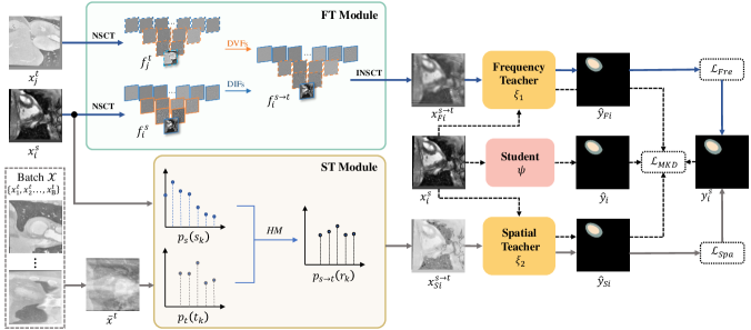
Figure 1: The training framework of our proposed method. The solid line represents the training process of the teacher networks, and the dashed line represents the training process of the multi-teacher distillation network.

Given source domain data $D_{s}={(x_{i}^{s},y_{i}^{s})}_{i=1}^{N_{s}}$, where $x_{i}^{s}\in{\mathbb{R}^{H\times{W}}}$ represents a source medical image with segmentation label $y_{i}^{s}\in{\mathbb{R}^{{n_{c}}\times{H}\times{W}}}$, and $n_{c}$ denotes the number of segmentation categories. Similarly, $D_{t}={(x_{j}^{t})}_{j=1}^{N_{t}}$ is the target domain data without segmentation labels. The objective of this paper is to train a segmentation model with $D_{s}$ and $D_{t}$ that performs well on the target domain.

The overall framework proposed in this paper is shown in Figure A1, where $x_{i}^{s}$ and $x_{j}^{t}$ are a source domain image and a target domain image, respectively, and $\bar{x}^{t}$ is the average image of a batch of target domain images. We use a frequency domain transfer (FT) module and a spatial domain transfer (ST) module to generate two sets of target-like images $x_{Fi}^{s\to{t}}$ and $x_{Si}^{s\to{t}}$, respectively. Each image set is used to train a teacher model, and the two teachers are then utilized to train a student model in a multi-teacher distillation framework for inference. The FT module takes $x_{i}^{s}$ and $x_{j}^{t}$ as inputs and each of them are decomposed into 15 frequency components (FCs) using NSCT, which are denoted as $f_{i}^{s}$ and $f_{j}^{t}$, respectively. We empirically identify domain invariant frequency components (DIFs) and domain variant frequency components (DVFs) in the NSCT components. The DVFs in $f_{i}^{s}$ are replaced with that in $f_{j}^{t}$, and the resulted source domain FCs are used to generate $x_{Fi}^{s\to{t}}$ using inverse NSCT. Details of the FT module are presented in Section 3.2.

In the ST module, we first calculate the normalized histogram $p_{s}(s_{k})$ of the source domain image $x_{i}^{s}$. At the same time, we randomly sample a batch of target domain images $\mathcal{X}=\{x_{1}^{t},x_{2}^{t}…,x_{B}^{t}\}\in{D_{t}}$ and calculate their average image $\bar{x}^{t}$ and its normalized histogram $p_{t}(t_{k})$. Then, $p_{s}(s_{k})$ is aligned with $p_{t}(t_{k})$ by histogram matching to obtain the transferred source domain image $x_{Si}^{s\to{t}}$. In this process, we introduce momentum updates to $p_{t}(t_{k})$ to make it change steadily. Details of the ST module are shown in Section 3.3.

We use $x_{Fi}^{s\to{t}}$ and $x_{Si}^{s\to{t}}$ to train two teacher models $\xi_{1}$ and $\xi_{2}$, respectively. Then, we utilize an entropy-based multi-teacher distillation strategy (Kwon et al. 2020) to integrate the information learned by the two teachers to train a student model for inference (see the dashed arrow data flow in Figure A1). Details of the distillation framework are presented in Section 3.4.

3.2 Frequency Domain Transfer Module

In this section, we will first briefly introduce NSCT for completeness and then present how it is used for frequency domain image transfer.

3.2.1 Non-Subsampled Contourlet Transform (NSCT)

NSCT can efficiently capture multi-scale visual information of images by decomposing an image into high-pass sub-bands representing details and low-pass sub-bands representing structural information (Zhu et al. 2019; Bhatnagar, Wu, and Liu 2013). Concretely, NSCT consists of two parts: a Non-Subsampled Pyramid (NSP) and a Non-Subsampled Directional Filter Bank (NSDFB), which are used to obtain multi-scale and multi-directional frequency components, respectively. We briefly introduce the three-layer NSCT used in this study here and more details can be found in the Supplementary Material Section 2.

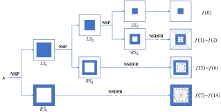
Figure 2: The detail of three-layer NSCT decomposition.

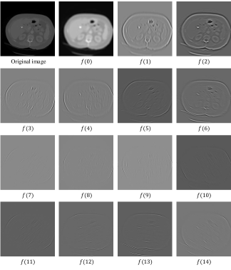
Figure 3: Example of NSCT decomposition of a abdominal MRI image.

As shown in Figure A2, for an input image $x$, a low-frequency sub-band image $LS_{1}$ and a high-frequency sub-band image $BS_{1}$ are obtained after NSP decomposition. The low-frequency sub-bands at the $l^{th}$ layer $LS_{l}$ will continue to be decomposed by NSP to obtain $LS_{l+1}$ and $BS_{l+1}$. Then, the high-frequency sub-bands $BS_{l}$ are further decomposed into $2^{l}$ multi-directional frequency sub-bands using NSDFB. After the $L$-level decomposition, the input image $x$ is transformed into a series of FCs, including the low-frequency sub-band $f(0)$, and a total number of $\sum_{l=1}^{L}2^{l}$ high-frequency sub-bands $f(1)\sim f(\sum_{l=1}^{L}2^{l})$.

Taking an abdominal MRI image $x_{i}^{s}$ as an example, we obtain its FCs $f_{i}^{s}$ by three-layer NSCT decomposition:

$$f_{i}^{s}={NSCT}(x_{i}^{s})=\{f_{i}^{s}(0),f_{i}^{s}(1),…,f_{i}^{s}(14)\}$$ (1)

The visualization of each sub-bund FC is shown in Figure 3. We can see that the FC of low frequency sub-band retain most of the semantic content of the image, while the FCs corresponding to high frequency sub-bands represent the structure and texture of the image in different directions.

3.2.2 NSCT-based Frequency Transfer Strategy

In order to narrow the domain gap using frequency components, we propose an NSCT-based frequency domain transfer strategy between the two domains.

First, for each source domain image, we decompose it into 15 FCs using NSCT, and then reconstruct a series of images from different combinations of these FCs. We train a baseline model using the original source domain images and train a transfer model using the images reconstructed from each FCs combination. Then DVFs and DIFs are identified according to the performance of all these models on a synthetic target domain data. Specifically, an improved performance over the baseline model implies that the rejected FCs in the corresponding combination are domain-variant, and removing these FCs can prevent the model from learning too many domain-variant features to facilitate domain adaptation. On the contrary, a decreased performance over the baseline model implies that the removed FCs are domain-invariant, and by retaining these components, the model is encouraged to learn domain-invariant features to facilitate domain adaptation.

Due to page limitation, the experimental details of identifying DIFs and DVFs are given in Supplementary Material Section 3, and we only give the results here, i.e. the FCs combination with the low-frequency $f_{i}^{s}(0)$ and the third-layer high-frequency components $f_{i}^{s}(7\sim 14)$ achieve the best results. Therefore, we consider the low-frequency FC and the third-layer FCs as DIFs, and the other FCs as DVFs.

After identifying the DVFs and DIFs, for a source domain image $x_{i}^{s}$, we keep its DIFs unchanged and replace its DVFs with that of a randomly selected target domain image to obtain the adapted FCs $f_{i}^{s\to{t}}$. Then inverse NSCT is applied on $f_{i}^{s\to{t}}$ to obtain the corresponding adapted image $x_{Fi}^{s\to{t}}$, which is used to train the frequency domain transfer-based segmentation teacher network $\xi_{1}$ with the loss function $\mathcal{L}_{Fre}$ defined as follows:

$$\mathcal{L}_{Fre}=\sum\left[\mathcal{L}_{CE}\left(\hat{y}_{Fi},y_{i}^{s}\right)+\mathcal{L}_{Dice}\left(\hat{y}_{Fi},y_{i}^{s}\right)\right]$$ (2)

where $\mathcal{L}_{CE}$ is the cross-entropy loss and $\mathcal{L}_{Dice}$ is the Dice loss. $\hat{y}_{Fi}$ is the predicted segmentation result.

3.3 Spatial Domain Transfer Module

In order to further reduce the domain gap, we utilize the spatial domain transfer module to generate another target-like image for model training by histogram matching (Gonzalez 2009). We propose to use batch momentum update to calculate an average histogram of a batch of target domain images for matching, rather than the entire target domain, which tends to smooth the target domain histogram and ignores the intensity variants (Yaras et al. 2021).

Concretely, given the source domain image $x_{i}^{s}$ and a batch of target domain image $\mathcal{X}=\{x_{1}^{t},x_{2}^{t}…,x_{B}^{t}\}$, we first normalize all these images to make them have integer intensity values falling in the range of $[0,L-1]$. The normalized histogram of $x_{i}^{s}$ is defined as $p_{s}(s_{k})=n_{k}/{HW}$, where $s_{k},k=0,1,…L-1$ represents the $k^{th}$ intensity value, and $n_{k}$ is the number of pixels with intensity $s_{k}$. Similarly, the histogram of the average target image of the current batch $\bar{x}^{t}=1/B\sum_{i=1}^{B}x_{i}^{t}$ is denoted as $p_{t}(t_{k})$.

Then, we use the source image histogram to find the histogram equalization transformation $T$ as follows, and round the obtained value ${\mu}_{k}$ to the integer range $[0,L-1]$.

$${\mu}_{k}=T\left(s_{k}\right)=\left(L-1\right)\sum_{j=0}^{k}{p_{s}(s_{j})}=\frac{L-1}{HW}\sum_{j=0}^{k}{n_{j}}$$ (3)

where $k=0,1,…,L-1$, $n_{j}$ is the number of pixels with intensity value $s_{j}$. Similarly, we can use the histogram of the average target intensity image $p_{t}(t_{k})$ to calculate its histogram equalization transformation function $G(t_{q}),q=0,1,…L-1$. Then round the resulting values $G(t_{q})$ to the integer range $[0,L-1]$ and store the values in a table.

$$G(t_{q})=(L-1)\sum_{i=0}^{q}p_{t}(t_{i})$$ (4)

For every value of $\mu_{k}$, we use the stored values of $G$ to find the corresponding value of $t_{q}$ so that $G(t_{q})$ is closest to $\mu_{k}$ and then we store these mappings from $\mu$ to $t$. Note that, if there are more than one values of $t_{q}$ satisfies the given $\mu_{k}$, we will choose the smallest value. Finally, we use the found mapping to map each equalized source domain image pixel value $\mu_{k}$ to the corresponding pixel with value $t_{q}$ and we can obtain the final histogram-matched image $x_{Si}^{s\to{t}}$.

In addition, for the update of the average intensity image of the current batch in the target domain, we use the cumulative average based on batch momentum update to slowly change the current average image.

$$\bar{x}_{i}^{t}=\eta\bar{x}_{i}^{t}+(1-\eta)\bar{x}_{i-1}^{t}$$ (5)

where $\eta$ is set as 0.7, $\bar{x}_{i}^{t}$ is the average target image of current batch $i$ and $\bar{x}_{i-1}^{t}$ is that of last batch. Finally, we input $x_{Si}^{s\to{t}}$ for training the second segmentation teacher network $\xi_{2}$, and the loss function $\mathcal{L}_{Spa}$ is defined as follows.

$$\mathcal{L}_{Spa}=\sum\left[\mathcal{L}_{CE}\left(\hat{y}_{Si},y_{i}^{s}\right)+\mathcal{L}_{Dice}\left(\hat{y}_{Si},y_{i}^{s}\right)\right]$$ (6)

where $\hat{y}_{Si}$ represents the predicted segmentation results.

3.4 Multi-teacher Knowledge Distillation for Domain Adaptation

Given the source domain data $D_{s}={(x_{i}^{s},y_{i}^{s})}_{i=1}^{N_{s}}$ and two trained teacher models $\xi_{1}$ and $\xi_{2}$, we train a student model for inference using the entropy-based dynamic multi-teacher distillation strategy (Kwon et al. 2020). As shown in Figure A1, we first input a source domain image $x_{i}^{s}$ into $\xi_{1}$ and $\xi_{2}$ to obtain the predicted segmentation category probability maps $\hat{y}_{Fi}$ and $\hat{y}_{Si}$, respectively. Then, we compute the entropy-based distillation loss to train the student network $\psi$ with $x_{i}^{s}$ and predict its probability maps $\hat{y}_{i}$. The loss function for training the student network is:

$$\mathcal{L}_{MKD}=\sum_{i=1}^{N_{s}}\{\alpha\left(\mathcal{L}_{CE}\left(\hat{y}_{i},y_{i}^{s}\right)+\mathcal{L}_{Dice}\left(\hat{y}_{i},y_{i}^{s}\right)\right)$$

$$+\omega_{KD}^{F}\mathcal{L}_{KD}\left(\hat{y}_{Fi},y_{i}^{s}\right)+\omega_{KD}^{S}\mathcal{L}_{KD}\left(\hat{y}_{Si},y_{i}^{s}\right)\}$$ (7)

$$\mathcal{L}_{KD} =\frac{1}{HW}\sum_{h=1}^{H}\sum_{w=1}^{W}KL\left(\sigma\left(\delta/\tau\right)||\sigma\left(\hat{y}_{i}/\tau\right)\right),$$

$$\omega_{KD}^{F} =1-\frac{H(\hat{y}_{Fi})}{H(\hat{y}_{Fi})+H(\hat{y}_{Si})},$$

$$\omega_{KD}^{S} =1-\frac{H(\hat{y}_{Si})}{H(\hat{y}_{Fi})+H(\hat{y}_{Si})}.$$ (8)

where $\delta=\hat{y}_{Fi},\hat{y}_{Si}$, $\sigma$ represents the softmax function, $KL$ denotes the Kullback-Leibler divergence, and $\tau$ is a temperature. $\alpha$ is a trade-off hyperparameter, which is set as 10. $H(\cdot)$ represents the entropy computation.

4 Experiments Results

4.1 Implementation Details

4.1.1 Datasets and Implementation Details

Abdominal Multi-organ Segmentation. We use the same Abdominal Multi-Organ dataset as SIFA (Chen et al. 2020), in which the publicly available CT data (Landman et al. 2015) with 30 volumes is the source domain data and the T2-SPIR MRI training data from ISBI 2019 CHAOS Challenge (Kavur et al. 2021) with 20 volumes is the target domain data. In each volume, a total of four abdominal organs are annotated, including liver, right (R.) kidney, left (L.) kidney, and spleen.

Multi-modality Cardiac Segmentation. We use Multi-Modality Whole Heart Segmentation (MMWHS) 2017 Challenge dataset (Zhuang and Shen 2016), which consists of 20 unaligned MRI and CT volumes with ground truth masks on each modality. We use the MRI and CT images as the source and target domain data, respectively. A total of four cardiac structures are annotated, including ascending aorta (AA), left atrium blood cavity (LAC), left ventricle blood cavity (LVC), and myocardium of the left ventricle (MYO).

Table 1: Quantitative results on cross-modality abdominal multi-organ segmentation. * represents our reproduced results.

Method	Dice ↑					ASD ↓
	Liver	R.kidney	L.kidney	Spleen	Average	Liver	R.kidney	L.kidney	Spleen	Average
Supervised	88.3	90.2	92.1	95.2	91.5	1.1	1.5	0.8	1.2	1.2
W/o adaptation	55.1	41.7	54.3	62.2	53.3	4.3	9.8	5.3	7.9	6.8
SynSeg-Net (TMI 18’)	87.2	90.2	76.6	79.6	83.4	2.8	0.7	4.8	2.5	2.7
AdaOutput (CVPR 18’)	85.8	89.7	76.3	82.2	83.5	1.9	1.4	3.0	1.8	2.1
CycleGAN (ICCV 17’)	88.8	87.3	76.8	79.4	83.1	2.0	3.2	1.9	2.6	2.4
CyCADA (ICML 18’)	88.7	89.3	78.1	80.2	84.1	1.5	1.7	1.3	1.6	1.5
Prior SIFA (AAAI 19’)	88.5	90.0	79.7	81.3	84.9	2.3	0.9	1.4	2.4	1.7
SIFA (TMI 20’)	90.0	89.1	80.2	82.3	85.4	1.5	0.6	1.5	2.4	1.5
SIFA (TMI 20’) *	88.8	88.6	79.8	82.6	85.0	1.8	1.0	1.3	2.7	1.7
FDA (CVPR 20’) *	85.2	85.2	78.2	80.2	82.2	1.8	1.2	2.4	3.2	2.2
Ours	89.6	90.0	90.3	87.0	89.2	1.4	1.5	1.2	2.0	1.5

Table 2: Quantitative results on cross-modality cardiac segmentation. * represents our reproduced results.

Method	Dice ↑					ASD ↓
	AA	LAC	LVC	MYO	Average	AA	LAC	LVC	MYO	Average
Supervised	94.1	91.9	94.5	85.7	91.6	1.5	0.7	1.4	1.5	1.3
W/o adaptation	60.4	37.5	38.2	48.0	46.0	9.4	16.2	15.1	11.5	13.1
PnP-AdaNet (Access 19’)	74.0	68.9	61.9	50.8	63.9	12.8	6.3	17.4	14.7	12.8
SynSeg-Net (TMI 18’)	71.6	69.0	51.6	40.8	58.2	11.7	7.8	7.0	9.2	8.9
AdaOutput (CVPR 18’)	65.2	76.6	54.4	43.6	59.9	17.9	5.5	5.9	8.9	9.6
CycleGAN (ICCV 17’)	73.8	75.7	52.3	28.7	57.6	11.5	13.6	9.2	8.8	10.8
CyCADA (ICML 18’)	72.9	77.0	62.4	45.3	64.4	9.6	8.0	9.6	10.5	9.4
Prior SIFA (AAAI 19’)	81.1	76.4	75.7	58.7	73.0	10.6	7.4	6.7	7.8	8.1
SIFA (TMI 20’)	81.3	79.5	73.8	61.6	74.1	7.9	6.2	5.5	8.5	7.0
FDA (CVPR 20’) *	80.8	76.2	75.9	60.5	73.4	8.2	5.8	9.2	9.3	8.1
ICMSC (MICCAI 21’)	85.6	86.4	84.3	72.4	82.2	2.4	3.3	3.4	3.2	3.1
CUDA (J-BHI 22’)	87.2	88.5	83.0	72.8	82.9	7.0	2.8	5.2	6.8	5.5
Ours	86.8	87.5	84.6	82.4	85.3	1.6	2.5	3.2	3.1	2.6

4.1.2 Evaluation Metrics. We employed two commonly-used metrics to evaluate the segmentation performance: the Dice similarity coefficient (Dice) and the Average Symmetric Surface Distance (ASD).

4.1.3 Experimental Setting. We applied TransUnet (Chen et al. 2021a) as the backbone of the two teacher networks and the student network. Our network was trained on an NVIDIA GTX 3090 GPU with a batch size of 32 and 50 epoch, using an ADAM optimizer with a learning rate of 1e-4. We used the official data split for training and testing, and more details are described in Supplementary Material Section 1.

4.2 Comparison Results

We compared our method with 10 existing state-of-the-art methods, including eight medical UDA methods: PnP-AdaNet (Dou et al. 2018), SynSeg-Net (Huo et al. 2018), CyCADA (Hoffman et al. 2018), Prior SIFA (Chen et al. 2019), SIFA (Chen et al. 2020), FDA (Yang and Soatto 2020), CUDA (Du and Liu 2021), ICMSC (Zeng et al. 2021) and two natural image UDA methods: AdaOutput (Tsai et al. 2018), CycleGAN (Zhu et al. 2017). Among them, we reproduced SIFA and FDA, and the results of the other studies are from their original papers. We also report the result of ‘W/o adaptation’ as the lower bound of UDA segmentation performance, which is obtained by directly using the model trained on the source domain data to the target domain without adaptation. Similarly, we report the result of ‘Supervised’ as the upper bound by training with labeled data in the target domain.

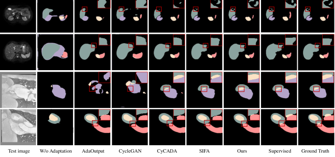
Figure 4: Visual comparison of segmentation results produced by different methods for abdominal multi-organ MRI images (the first and second rows) and cardiac CT images (the third and fourth rows). The liver, right kidney, left kidney and spleen are colored in blue, purple, yellow and red respectively. The cardiac structures of AA, LAC, LVC and MYO are colored in red, purple, yellow and blue respectively.

4.2.1 Abdominal Multi-organ Image Segmentation

The results of abdominal multi-organ segmentation are shown in Table 1. Our proposed method achieves the best average Dice and average ASD, and it outperforms the comparing methods by a large margin in terms of average Dice. In the four organs, our method achieves the best performance on three of them in terms of both Dice and ASD. Without adaptation, the trained model can only achieve an average Dice of 53.3$\%$ and an average ASD of 6.8 on the target domain images. When our proposed UDA method is used, the Dice is increased significantly by 35.9$\%$ and the ASD is reduced by 5.3. Noteworthily, the average Dice of our method is only 2.3$\%$ lower than the supervised upper bound. The visualization results are shown in Figure 4 (Rows 1-2). Without adaptation, the network can barely predict correct abdominal organs. The segmentation results of AdaptOut and CycleGAN show much noise and incorrect prediction masks. Our proposed method produces more precise segmentation results than CyCADA and SIFA.

4.2.2 Multi-modality Cardiac Segmentation

The results of multi-modality cardiac segmentation are shown in Table 2. Again, our method achieves the best average Dice and average ASD and the margin over comparing method are fairly large in terms of both Dice and ASD. Compared to ‘W/o adaption’, our method can increase the average Dice by 39.3$\%$ and reduce the average ASD by 10.5. Our method achieves the best performance on all four parts of heart in terms of ASD and on three parts in terms of Dice. The visualization results are shown in Figure 4 (Rows 3-4). Compared with other UDA methods, our proposed method generates more accurate predicted cardiac structures.

4.3 Ablation Studies on Key Components

We conducted ablation studies on each key component proposed in our adaptation framework on both datasets and the results are shown in Table 3, where ‘+ Spatial Transfer’ and ‘+ Frequency Transfer’ means training the segmentation model with spatial domain and frequency domain transferred images, respectively, and ‘+ S$\&$F Training’ means mixing transferred images from both spatial and frequency domains to train the segmentation model. Compared with ‘W/o adaptation’, both the spatial transfer and the frequency transfer strategy can significantly improve the segmentation performance on target domains. These results demonstrate the effectiveness of both transfer strategies. While simple mixing the spatial and frequency transferred images for model training is not effective, employing the multi-teacher knowledge distillation framework can improve the performance on target domains. These results indicate the effectiveness of the proposed multi-teacher distillation framework. The visualization of methods represent in Supplementary Material Section 4.

Table 3: The ablation studies on the effectiveness of key components.

Method	Abdominal		Cardiac
	Dice ↑	ASD ↓	Dice ↑	ASD ↓
W/o adaptation	53.3	6.8	46.0	13.1
+ Spatial Transfer(S)	88.6	1.4	83.7	3.2
+ Frequency Transfer(F)	87.3	2.0	84.6	2.4
+ S&F Trainning	88.4	1.9	83.9	3.6
Proposed Framework	89.2	1.5	85.3	2.6

Figure 5 visualizes the segmentation results of one example in each dataset in the ablation study. Generally speaking, every UDA setting shows good segmentation results. With the proposed framework, the segmentation results are more similar to the ground truth.

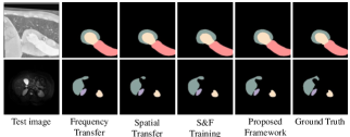
Figure 5: Visualization results of cardiac parts and abdominal organs using different settings in the ablation study.

4.4 Ablation Study on Different Histogram Matching Strategies

To reduce the style bias between the source and the target domains, we propose to use a histogram matching strategy based on batch momentum update to generate target-like images in the spatial domain. To validate the effectiveness of the batch momentum update-based histogram matching strategy, we conducted ablation experiments on different ways of target domain data selection in the histogram matching process. We experimented on four histogram calculation methods, including calculating the average histogram of the entire target domain data, randomly selecting the histogram of a single target domain image, calculating the average histogram of the current batch of target images and our proposed batch momentum update based histogram matching. The experiment results on the cardiac dataset shown in Table 4 indicate that our proposed method achieves the best segmentation performance on target domain.

Table 4: Experimental results of different histogram matching strategies on cardiac datasets (source domain: MRI, target domain: CT)

Method	Dice ↑	ASD ↓
Entire target domain images	81.5	3.4
Single target image	82.8	3.1
Batch average-based	83.4	3.3
Batch momentum update-based	83.7	3.2

5 Conclusion

In this paper, we propose a novel multi-teacher distillation framework for UDA based on frequency domain and spatial domain image transfer. In the frequency domain, we use NSCT to decompose images into 15 FCs and generate target-like images by combining selected FCs from the source and the target domain images for model training. In the spatial domain, we utilize histogram matching based on batch momentum update strategy to generate another set of target-like images for model training. Two teacher models are obtained with the frequency domain transferred images and the spatial domain transferred images, and a student model is then trained for inference under a multi-teacher distillation framework. Comparisons to existing methods and ablation studies validate the effectiveness of our proposed method. The idea of combining spatial and frequency domain transfer strategies in a multi-teacher distillation framework have the potential to be used in other UDA tasks.

Appendix A Appendix

A.1 Implementation Details

A.1.1 Experimental Setting

We applied TransUNet (Chen et al. 2021a) as the backbone of the two teacher networks and the student network. Our network was trained on an NVIDIA GTX 3090 GPU with a batch size of 32 and 50 epoch, using an Adam optimizer and a cosine annealing learning rate adjustment strategy with a learning rate of 1e-4 and a weight decay of 5e-4. We used the official data split for training and testing on two commonly-used segmentation datasets. For these two datasets, we split both source and target domain datasets with 80% data for training and 20% for testing according to their original setting. When training the two teacher networks, the training set of the source domain with different transfer strategies was used to optimize the model and then test on target domain testing set. After finishing the training of the two teachers, we used the same dataset splitting for training on source domain training set and testing on target domain.

A.1.2 Implementation Algorithms

The specific implementation algorithms of two teacher models training phase and multi-teacher distillation process are shown in Algorithm 1 and Algorithm 2, respectively.

Algorithm 1 Training process of the two teacher models.

0:  Source dataset $D_{s}=\{(x_{i}^{s},y_{i}^{s})\}_{i=1}^{N_{s}}$, target dataset $D_{t}=\{x_{j}^{t}\}_{j=1}^{N_{t}}$, model based on frequency transfer $\xi_{1}$, model based on spatial transfer $\xi_{2}$. % Frequency based Transfer Strategy

1:  for epoch $<$ $N$ do

2:     for $x_{i}^{s}\in D_{s}$ do

3:        Randomly select a target domain image $x_{j}^{t}\in D_{t}$.

4:        $f_{i}^{s}=NSCT(x_{i}^{s}),f_{j}^{t}=NSCT(x_{j}^{t}).$

5:        Get frequency components $f_{i}^{s\to t}$ and image $x_{Fi}^{s\to t}$ after frequency transfer.

6:        Generate the predicted mask $\hat{y}_{Fi}^{s\to t}=\xi_{1}\left(x_{Fi}^{s\to t}\right)$.

7:        Optimize model $\xi_{1}$ with $\mathcal{L}_{Fre}$.

8:     end for

9:  end for% Spatial based Transfer Strategy for Style alignment

10:  for epoch $<$ $N$ do

11:     for $i^{th}$ batch $\mathcal{X}_{s}=\{x_{1}^{s},x_{2}^{s},\ldots,x_{B}^{s}\}\in D_{S}$ and $\mathcal{X}_{t}=\{x_{1}^{t},x_{2}^{t},\ldots,x_{B}^{t}\}\in D_{t}$ do

12:        Compute the target domain average grayscale image $\bar{x}_{i}^{t}=1/B\sum_{j=1}^{B}x_{j}^{t}$ .

13:        for  $x_{j}^{s}\in\mathcal{X}_{s}$ do

14:           Generate transferred image with momentum histogram matching $x_{Sj}^{s\to t}=match\_histogram(x_{j}^{s},\bar{x}_{i}^{t})$

15:           if $i>1$ then

16:              Update $\bar{x}_{i}^{t}$ with momentum $\eta$:$\bar{x}_{i}^{t}=\eta\bar{x}_{i}^{t}+(1-\eta)\bar{x}_{i-1}^{t}$

17:           end if

18:           Generate the predicted mask $\hat{y}_{Sj}^{s\to t}=\xi_{2}(x_{Sj}^{s\to t})$;

19:           Optimize model $\xi_{2}$ with $\mathcal{L}_{Spa}$.

20:        end for

21:     end for

22:  end for

22:  Model $\xi_{1}$ based on frequency transfer and model $\xi_{2}$ based on histogram matching.

Algorithm 2 Training process of multi-teacher distillation.

0:  Source dataset $D_{s}=\{(x_{i}^{s},y_{i}^{s})\}_{i=1}^{N_{s}}$, teacher model $\xi_{1},\xi_{2}$, student model $\psi$.

1:  for epoch $<$ $N$ do

2:     for $x_{i}^{s}\in D_{s}$ do

3:        Generate the predicted masks $\hat{y}_{Fi}=\xi_{1}(x_{Fi}^{s\to t}),\hat{y}_{Si}=\xi_{2}(x_{Si}^{s\to t}),\hat{y}_{i}=\psi(x_{i}^{s})$

4:        Optimize the student model $\psi$ with $\mathcal{L}_{MKD}$.

5:     end for

6:  end for

6:  Student model $\psi$.

A.2 Non-Subsampled Contourlet Transform

Non-Subsampled Contourlet transform (NSCT) can efficiently capture multi-scale visual information of images by decomposing the image into high-pass sub-bands representing details and low-pass sub-bands representing structural information (Zhu et al. 2019; Bhatnagar, Wu, and Liu 2013). Concretely, NSCT consists of two parts: a Non-Subsampled Pyramid (NSP) and a Non-Subsampled Directional Filter Bank (NSDFB) shown in Figure A1, which are used to obtain multi-scale and multi-directional frequency components, respectively. We briefly introduce the three-layer NSCT used in this study here.

In NSP process, $H_{0}(z)$ and $H_{1}(z)$ represent low-pass filter and high-pass filter, respectively. For an input image $x$, NSP first decomposes it into a low-pass image $LS_{1}$ and a band-pass image $BS_{1}$ at the first layer using $H_{0}(z)$ and $H_{1}(z)$. $LS_{1}$ is further decomposed by NSP in layer two as $LS_{2}$ and $BS_{2}$. After $L$ times of NSP decompositions, the input image $x$ is decomposed into one low-pass image $LS_{L}$ and $L$ sub-band images $BS_{l},l=1,2,…,L$.

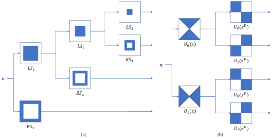
Figure A1: The details of NSP (left) and NSDFB (right).

NSDFB consists of non-subsampled directional filters including fan filters $U(z)$ and quadrature filters $U(z^{D})$. For the band-pass image in $l^{th}$ layer, NSDFB decompose it into $2^{l}$ frequency components (FCs) in different directions. Thus, after $L$-level NSCT decomposition, the input image $x$ is transformed into a series of FCs, including $f(0)$ corresponding to the low-frequency sub-band $LS_{L}$, and band-pass FCs $f(1)\sim f(\sum_{l=1}^{L}2^{l})$ corresponding to $L$ high frequency sub-bands $BS_{l},l=1,2,…,L$.

A.3 Empirical Experiments for DVFs and DIFs Identification

In the pre-experiment, we perform NSCT and FCs transfer on the source and target domain images respectively, and then identify DIFs and DVFs according to the results using the transferred images. However, since the label of target domain images are not available, we match the histogram of the source domain image to that of the target ones to obtain target-like, labeled source domain image as ”synthetic target domain data” for pre-experiment.

First, for each source domain image, we decompose it into 15 FCs using NSCT, and then reconstruct a series of images from different combinations of these FCs. The combination of frequency domain components is achieved by a band-stop filter, where the blocked frequency domain components are the ‘rejected FCs’. We train a baseline model using the original source domain images and train a transfer model using the images reconstructed from each FC combination. Then DVFs and DIFs are identified according to the performance of all these models on a synthetic target domain data. Specifically, an improved performance over the baseline model implies that the rejected FCs in the corresponding combination are domain-variant, and removing these FCs can prevent the model from learning too many domain-variant features to facilitate domain adaptation. On the contrary, a decreased performance over the baseline model implies that the removed FCs are domain-invariant, and by retaining these components, the model is encouraged to learn domain-invariant features to facilitate domain adaptation. In view of this insight, we conducted the experiments on synthetic target domain datasets because we have no access to segmentation ground truth in the target domain. Concretely, we use histogram matching strategy as described in original paper Section 3.3 to generate target style-like source images as synthetic target domain dataset. Then, we train the model using the new source images with different combination of FCs and test on synthetic target domain datasets in two applications.

The results of different FCs combinations on cardiac and abdominal multi-organ datasets are shown in Table A1.

Table A1: Comparison results of different FCs combinations on cardiac and abdominal multi-organ datasets.

No.	FCs	Cardiac Dice (%) ↑		Abdominal Dice (%) ↑
		src val	trgt val	src val	trgt val
Baseline	[0,15]	73.56	60.42	78.45	68.25
1	[0,1]	49.95	41.15	58.65	44.26
2	[1,3]	67.74	58.23	65.25	52.32
3	[3,7]	75.13	58.56	79.61	67.25
4	[7,14]	71.54	62.65	75.74	71.63
5	[0,1], [1,3]	72.02	59.98	72.84	64.62
6	[0,1], [3,7]	70.16	60.25	73.69	68.86
7	[0,1], [7,14]	77.32	64.85	80.17	72.54

From Table A1, we can see that compared to Baseline (full FCs), when we keep the low-frequency FC ([0,1]) and the third-layer FCs ([7,14]), the segmentation results on synthetic target domain validation dataset achieve improved and best performance on both applications. Therefore, we consider these FCs as DIFs and the rest as DVFs. The low-frequency component represents the shape and semantics of the image, which is important for semantic information learning. However, the segmentation results of only preserving low-frequency component show poor performance, which demonstrates the significance of the high-frequency components containing details and textures. When we keep different high-level FCs combined with low-level FC, the performance is consistently improved compared with the results only with different high-level FCs and only with low-level FC, which both validates the importance of semantics containing in low-level FC and details containing in high-level FCs.

A.4 Visualization results of Different Transfer Strategies

Examples of adapted images with different transfer strategies are visualized in Figure A2. We can see that the appearance of the source images is indeed adapted into target domains in different perspectives. In the frequency domain, we are expected to randomize the domain-variant frequency components while keeping the domain-invariant components unchanged. In the spatial domain, we are expected to align their style bias between different domains.

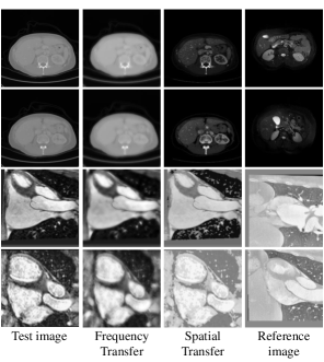
Figure A2: Examples of adapted images with different transfer strategies. The first two rows are from chaos CT images, and the last two rows are from cardiac MRI images.

References

- AlBadawy, Saha, and Mazurowski (2018) AlBadawy, E. A.; Saha, A.; and Mazurowski, M. A. 2018. Deep learning for segmentation of brain tumors: Impact of cross-institutional training and testing. Medical Physics, 45(3): 1150–1158.
- Bhatnagar, Wu, and Liu (2013) Bhatnagar, G.; Wu, Q. J.; and Liu, Z. 2013. Directive contrast based multimodal medical image fusion in NSCT domain. IEEE Transactions on Multimedia, 15(5): 1014–1024.
- Chen et al. (2019) Chen, C.; Dou, Q.; Chen, H.; Qin, J.; and Heng, P.-A. 2019. Synergistic image and feature adaptation: Towards cross-modality domain adaptation for medical image segmentation. In Proceedings of the AAAI Conference on Artificial Intelligence, volume 33, 865–872.
- Chen et al. (2020) Chen, C.; Dou, Q.; Chen, H.; Qin, J.; and Heng, P. A. 2020. Unsupervised bidirectional cross-modality adaptation via deeply synergistic image and feature alignment for medical image segmentation. IEEE Transactions on Medical Imaging, 39(7): 2494–2505.
- Chen et al. (2021a) Chen, J.; Lu, Y.; Yu, Q.; Luo, X.; Adeli, E.; Wang, Y.; Lu, L.; Yuille, A. L.; and Zhou, Y. 2021a. Transunet: Transformers make strong encoders for medical image segmentation. arXiv preprint arXiv:2102.04306.
- Chen et al. (2021b) Chen, S.; Jia, X.; He, J.; Shi, Y.; and Liu, J. 2021b. Semi-supervised domain adaptation based on dual-level domain mixing for semantic segmentation. In Proceedings of the IEEE/CVF Conference on Computer Vision and Pattern Recognition, 11018–11027.
- Csurka et al. (2017) Csurka, G.; et al. 2017. Domain adaptation in computer vision applications. Springer.
- Dou et al. (2018) Dou, Q.; Ouyang, C.; Chen, C.; Chen, H.; Glocker, B.; Zhuang, X.; and Heng, P.-A. 2018. Pnp-adanet: Plug-and-play adversarial domain adaptation network with a benchmark at cross-modality cardiac segmentation. arXiv preprint arXiv:1812.07907.
- Du and Liu (2021) Du, X.; and Liu, Y. 2021. Constraint-Based Unsupervised Domain Adaptation Network for Multi-Modality Cardiac Image Segmentation. IEEE Journal of Biomedical and Health Informatics, 26(1): 67–78.
- Ghafoorian et al. (2017) Ghafoorian, M.; Mehrtash, A.; Kapur, T.; Karssemeijer, N.; Marchiori, E.; Pesteie, M.; Guttmann, C. R.; Leeuw, F.-E. d.; Tempany, C. M.; Ginneken, B. v.; et al. 2017. Transfer learning for domain adaptation in MRI: Application in brain lesion segmentation. In International Conference on Medical Image Computing and Computer-assisted Intervention, 516–524. Springer.
- Gonzalez (2009) Gonzalez, R. C. 2009. Digital image processing. Pearson Education India.
- Guan and Liu (2021) Guan, H.; and Liu, M. 2021. Domain adaptation for medical image analysis: a survey. IEEE Transactions on Biomedical Engineering, 69(3): 1173–1185.
- He et al. (2021) He, J.; Jia, X.; Chen, S.; and Liu, J. 2021. Multi-source domain adaptation with collaborative learning for semantic segmentation. In Proceedings of the IEEE/CVF Conference on Computer Vision and Pattern Recognition, 11008–11017.
- Hoffman et al. (2018) Hoffman, J.; Tzeng, E.; Park, T.; Zhu, J.-Y.; Isola, P.; Saenko, K.; Efros, A.; and Darrell, T. 2018. Cycada: Cycle-consistent adversarial domain adaptation. In International Conference on Machine Learning, 1989–1998. Pmlr.
- Huang et al. (2021) Huang, J.; Guan, D.; Xiao, A.; and Lu, S. 2021. Fsdr: Frequency space domain randomization for domain generalization. In Proceedings of the IEEE/CVF Conference on Computer Vision and Pattern Recognition, 6891–6902.
- Huo et al. (2018) Huo, Y.; Xu, Z.; Moon, H.; Bao, S.; Assad, A.; Moyo, T. K.; Savona, M. R.; Abramson, R. G.; and Landman, B. A. 2018. Synseg-net: Synthetic segmentation without target modality ground truth. IEEE Transactions on Medical Imaging, 38(4): 1016–1025.
- Kavur et al. (2021) Kavur, A. E.; Gezer, N. S.; Barış, M.; Aslan, S.; Conze, P.-H.; Groza, V.; Pham, D. D.; Chatterjee, S.; Ernst, P.; Özkan, S.; et al. 2021. CHAOS challenge-combined (CT-MR) healthy abdominal organ segmentation. Medical Image Analysis, 69: 101950.
- Kwon et al. (2020) Kwon, K.; Na, H.; Lee, H.; and Kim, N. S. 2020. Adaptive knowledge distillation based on entropy. In ICASSP 2020-2020 IEEE International Conference on Acoustics, Speech and Signal Processing, 7409–7413. IEEE.
- Landman et al. (2015) Landman, B.; Xu, Z.; Igelsias, J.; Styner, M.; Langerak, T.; and Klein, A. 2015. Miccai multi-atlas labeling beyond the cranial vault–workshop and challenge. In Proc. MICCAI Multi-Atlas Labeling Beyond Cranial Vault—Workshop Challenge, volume 5, 12.
- Ma et al. (2021) Ma, H.; Lin, X.; Wu, Z.; and Yu, Y. 2021. Coarse-to-fine domain adaptive semantic segmentation with photometric alignment and category-center regularization. In Proceedings of the IEEE/CVF Conference on Computer Vision and Pattern Recognition, 4051–4060.
- Ma et al. (2022) Ma, X.; Yuan, J.; Chen, Y.-w.; Tong, R.; and Lin, L. 2022. Attention-based cross-layer domain alignment for unsupervised domain adaptation. Neurocomputing, 499: 1–10.
- Nam et al. (2021) Nam, H.; Lee, H.; Park, J.; Yoon, W.; and Yoo, D. 2021. Reducing domain gap by reducing style bias. In Proceedings of the IEEE/CVF Conference on Computer Vision and Pattern Recognition, 8690–8699.
- Shen et al. (2020) Shen, R.; Yao, J.; Yan, K.; Tian, K.; Jiang, C.; and Zhou, K. 2020. Unsupervised domain adaptation with adversarial learning for mass detection in mammogram. Neurocomputing, 393: 27–37.
- Toldo et al. (2020) Toldo, M.; Maracani, A.; Michieli, U.; and Zanuttigh, P. 2020. Unsupervised domain adaptation in semantic segmentation: a review. Technologies, 8(2): 35.
- Tsai et al. (2018) Tsai, Y.-H.; Hung, W.-C.; Schulter, S.; Sohn, K.; Yang, M.-H.; and Chandraker, M. 2018. Learning to adapt structured output space for semantic segmentation. In Proceedings of the IEEE/CVF Conference on Computer Vision and Pattern Recognition, 7472–7481.
- Wollmann, Eijkman, and Rohr (2018) Wollmann, T.; Eijkman, C.; and Rohr, K. 2018. Adversarial domain adaptation to improve automatic breast cancer grading in lymph nodes. In 2018 IEEE 15th International Symposium on Biomedical Imaging, 582–585. IEEE.
- Xing et al. (2020) Xing, F.; Cornish, T. C.; Bennett, T. D.; and Ghosh, D. 2020. Bidirectional mapping-based domain adaptation for nucleus detection in cross-modality microscopy images. IEEE Transactions on Medical Imaging, 40(10): 2880–2896.
- Xu et al. (2021) Xu, Q.; Zhang, R.; Zhang, Y.; Wang, Y.; and Tian, Q. 2021. A fourier-based framework for domain generalization. In Proceedings of the IEEE/CVF Conference on Computer Vision and Pattern Recognition, 14383–14392.
- Yang and Soatto (2020) Yang, Y.; and Soatto, S. 2020. Fda: Fourier domain adaptation for semantic segmentation. In Proceedings of the IEEE Conference on Computer Vision and Pattern Recognition, 4085–4095.
- Yaras et al. (2021) Yaras, C.; Huang, B.; Bradbury, K.; and Malof, J. M. 2021. Randomized Histogram Matching: A Simple Augmentation for Unsupervised Domain Adaptation in Overhead Imagery. arXiv preprint arXiv:2104.14032.
- Zeng et al. (2021) Zeng, G.; Lerch, T. D.; Schmaranzer, F.; Zheng, G.; Burger, J.; Gerber, K.; Tannast, M.; Siebenrock, K.; and Gerber, N. 2021. Semantic consistent unsupervised domain adaptation for cross-modality medical image segmentation. In International Conference on Medical Image Computing and Computer Assisted Intervention, 201–210. Springer.
- Zhang et al. (2019) Zhang, J.; Liu, M.; Pan, Y.; and Shen, D. 2019. Unsupervised conditional consensus adversarial network for brain disease identification with structural MRI. In International Workshop on Machine Learning in Medical Imaging, 391–399. Springer.
- Zhu et al. (2017) Zhu, J.-Y.; Park, T.; Isola, P.; and Efros, A. A. 2017. Unpaired image-to-image translation using cycle-consistent adversarial networks. In Proceedings of the IEEE International Conference on Computer Vision, 2223–2232.
- Zhu et al. (2019) Zhu, Z.; Zheng, M.; Qi, G.; Wang, D.; and Xiang, Y. 2019. A Phase Congruency and Local Laplacian Energy Based Multi-Modality Medical Image Fusion Method in NSCT Domain. IEEE Access, 7: 20811–20824.
- Zhuang and Shen (2016) Zhuang, X.; and Shen, J. 2016. Multi-scale patch and multi-modality atlases for whole heart segmentation of MRI. Medical Image Analysis, 31: 77–87.