Incremental Spectral Learning in Fourier Neural Operator

Abstract

Recently, neural networks have proven their impressive ability to solve partial differential equations (PDEs). Among them, Fourier neural operator (FNO) has shown success in learning solution operators for highly non-linear problems such as turbulence flow. FNO learns weights over different frequencies and as a regularization procedure, it only retains frequencies below a fixed threshold. However, manually selecting such an appropriate threshold for frequencies can be challenging, as an incorrect threshold can lead to underfitting or overfitting. To this end, we propose Incremental Fourier Neural Operator (IFNO) that incrementally adds frequency modes by increasing the truncation threshold adaptively during training. We show that IFNO reduces the testing loss by more than 10% while using 20% fewer frequency modes, compared to the standard FNO training on the Kolmogorov Flow (with Reynolds number up to 5000) under the few-data regime.

1 Introduction

Deep learning has been widely used in a variety of fields, from image recognition and natural language processing to solving scientific problems in physics, chemistry, and biology (Jumper et al., 2021; Degrave et al., 2022; Zvyagin et al., 2022). One of the most promising directions is using neural networks to solve partial differential equations (PDEs), which are ubiquitous in many scientific fields. In particular, the Fourier neural operator (FNO), recently proposed by Li et al. (a), achieves state-of-the-art performance in solving PDEs.

FNO is designed for solving PDEs by learning the solution operator that maps the input (initial and boundary conditions) to the output (solution functions). Along with other neural operators, FNO is a universal approximator that can represent any continuous solution operator (Kovachki et al., 2021). It has shown tremendous impact in solving highly non-linear PDE problems such as weather forecast (Pathak et al., 2022), material plasticity (Liu et al., 2022), and carbon storage (Wen et al., 2022).

FNO enjoys a property known as discretization-invariance, which allows FNO to train and test on different resolutions of PDE problems without significant performance degradation, while conventional neural networks do not. The discretization-invariance is achieved by parameterizing the linear transforms directly over the Fourier space followed by non-linearity.

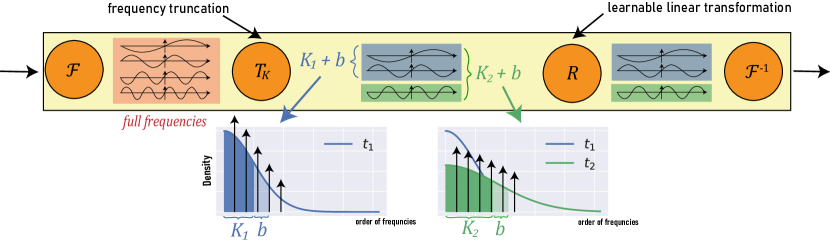
Figure 1: Top: Fourier convolution operator in FNO. After the Fourier transform $\mathcal{F}$, the layer truncates the full set of input frequencies to the $K$ lowest ones using a fixed truncation $T_{k}$, and then it applies a learnable linear transformation $R$ before mapping the frequencies back to the linear space using $\mathcal{F}^{-1}$. Previous method (Li et al., a) picks a fixed $K$ throughout the entire training. Bottom: incremental augmentation of frequency modes. Solid areas represent how much information in the spectrum is explained by the current modes $K_{t}$ at iteration $t$. From iteration $t_{1}$ to $t_{2}$, IFNO adds $K_{2}-K_{1}$ frequency modes to ensure the ratio of the explained information is greater than a certain threshold $\alpha$.

Capture the right frequency spectral is a central concern for both PDEs and machine learning. For most PDE systems, the large-scale, low-frequency components usually have larger magnitudes than small-scale, high-frequency components in PDEs. Therefore, as a regularization, FNO consists of a frequency truncation $T_{K}$ in each layer that only allows the lowest $K$ Fourier modes to propagate input information, as shown in Figure 1. The truncation $T_{K}$ encourages the learning of low-frequency components in PDEs, which is also related to the well-known phenomenon of implicit spectral bias. The implicit spectral bias suggests that neural networks trained by gradient descent implicitly prioritize learning low-frequency functions (Rahaman et al., ). It provides an implicit regularization effect that encourages a neural network to converge to a low-frequency and “simple” solution, among all possible candidates. This helps to explain why deep neural networks can generalize well while having considerably more learnable parameters than training samples.

However, it is still a challenge to explicitly apply an additional spectral regularization to further enhance the generalization in practice. Consider a weight matrix $M$ in a linear layer as an example. Traditional spectral regularization methods try to suppress small eigenvalues of $M$ to form it as a low-pass filter (Gerfo et al., 2008). These methods require expensive computation (such as performing eigen-decomposition at each training iteration) to access the eigenvalues of $M$, which makes them impractical for the training of large-scale neural networks.

It’s easier to measure the spectral bias in FNO without the need for expensive eigen-decomposition, since the frequency truncation $T_{K}$ is able to directly measure and control the spectrum of the model. For example, Li et al. (a) fix $K$ lowest frequencies through the entire training. However, it is challenging to select an appropriate $K$, as it is task-dependent and requires careful hyperparameter tuning. Setting $K$ too small will result in too few frequency modes, such that it delivers sufficient information for learning the solution operator, resulting in underfitting. On the other hand, a larger $K$ increases the parameter size and encourages FNO to interpolate the high-frequency noise. This results in overfitting while being computationally expensive.

Our work: we propose the incremental Fourier neural operator (IFNO) to address the above challenges. IFNO automatically increments the number of frequency modes $K$ during training. It adds a new batch of frequency modes whenever a certain quantity, known as the explained ratio, exceeds a certain threshold. The explained ratio characterizes the amount of information in the underlying spectrum that the current set of modes can explain. A small explained ratio indicates that the current modes are insufficient to represent the spectrum, and thus more high-frequency modes should be added, as illustrated in Figure 1.

Our contributions are summarized as follows:

1. We propose IFNO that incrementally augments the number of frequency modes $K$ during the training. This addresses the challenge of selecting an appropriate $K$ in the previous studies.

2. IFNO serves as a dynamic spectral regularization, which yields better generalization performance, especially in the few-data regime.

3. IFNO significantly improves training and inference efficiency, as it requires fewer frequency modes than the standard FNO without damaging any performance.

4. We evaluate IFNO on a variety of PDE problems. They include Naiver-Stokes Equation on Kolmogorov Flow, where we show that IFNO reduces more than 10% testing loss while using 20% fewer frequency modes compared to the standard FNO under few-data regime.

2 Fourier Neural Operator

FNO proposed by Li et al. (a) serves as a family of neural operators, which are formulated as a generalization of standard deep neural networks to operator setting (Li et al., b). A neural operator learns a mapping between two infinite dimensional spaces from a finite collection of observed input-output pairs. Let $D$ be a bounded, open set and $\mathcal{A}$ and $\mathcal{U}$ be separable Banach spaces of functions of inputs and outputs.

We want to learn a neural operator $\mathcal{G}_{\theta}:\mathcal{A}\times\theta\to\mathcal{U}$ that maps any initial condition $a\in\mathcal{A}$ to its solution $u\in\mathcal{U}$. The neural operator $\mathcal{G}_{\theta}$ composes linear integral operator $\mathcal{K}$ with pointwise non-linear activation function $\sigma$ to approximate highly non-linear operators.

Definition 2.1 (Neural operator).

The neural operator $\mathcal{G}_{\theta}$ is defined as follows:

$$\mathcal{G}_{\theta}:=\mathcal{Q}\circ\left(W_{L}+\mathcal{K}_{L}\right)\circ\cdots\circ\sigma\left(W_{1}+\mathcal{K}_{1}\right)\circ\mathcal{P},$$

where $\mathcal{P},\mathcal{Q}$ are the pointwise neural networks that encode the lower dimension function into higher dimensional space and decode the higher dimension function back to the lower dimensional space. The model stack $L$ layers of $\sigma\left(W_{l}+\mathcal{K}_{l}\right)$ where $W_{l}$ are pointwise linear operators (matrices), $\mathcal{K}_{l}$ are integral kernel operators, and $\sigma$ are fixed activation functions. The parameters $\theta$ consist of all the parameters in $\mathcal{P},\mathcal{Q},W_{l},\mathcal{K}_{l}$.

Li et al. (a) proposes FNO that adopts a convolution operator for $\mathcal{K}$ as shown in Figure 1, which obtains state-of-the-art results for solving PDE problems.

Definition 2.2 (Fourier convolution operator).

Define the Fourier convolution operator $\mathcal{K}$ as follows:

$$\left(\mathcal{K}v_{t}\right)(x)=\mathcal{F}^{-1}\left(R\cdot T_{K}\left(\mathcal{F}v_{t}\right)\right)(x)\quad\forall x\in D,$$

where $\mathcal{F}$ and $\mathcal{F}^{-1}$ are the Fourier transform and its inverse, $R$ is a learnable transformation and $T_{K}$ is a fixed truncation that restricts the input to lowest $K$ Fourier modes.

FNO is discretization-invariant, such that the model can produce a high-quality solution for any query points, potentially not in the training grid. In other words, FNO can be trained on low-resolution but generalizes to high-resolution. This property is highly desirable as it allows a transfer of solutions between different grid resolutions and discretizations.

Frequency truncation.

To ensure discretization invariance, FNO truncates the Fourier series $\mathcal{\hat{F}}v$ at a maximal number of modes $K$ using $T_{K}$. In this case, for any discrete frequency mode $k\in\{1,...,K\}$, we have $\mathcal{\hat{F}}v(k)\in\mathbb{C}^{\textrm{C}}$ and $R(k)\in\mathbb{C}^{\textrm{C}\times\textrm{C}}$, where C is the channel dimension of the input $v$. The size of linear parameterization $R$ depends on $K$. For example, $R$ has the shape of $K^{d}\times\textrm{C}\times\textrm{C}$ for a $d$-dimensional problem. We also denote the modes $1,...,K$ as the effective frequency modes. In the standard FNO, Li et al. (a) view $K$ as an additional hyperparameter to be tuned for each problem.

Frequency strength.

As $R(k)$ reflects how the frequency mode $k$ is transformed, we can measure the strength of transforming the frequency mode $k$ by the Frobenius norm of $R(k)$, such that:

$$S_{k}=\sum_{i}^{\textrm{C}}\sum_{j}^{\textrm{C}}R_{k,i,j}^{2},$$ (1)

where $S_{k}$ denotes the strength of the $k$-th frequency mode. A smaller $S_{k}$ indicates that the $k$-th frequency mode is less important for the output.

3 The importance of low-frequency modes

In this section, we will explain why frequency truncation is necessary for FNO, through the discussion of the importance of low-frequency modes in learning neural networks and the nature of PDEs.

3.1 Implicit spectral bias in neural networks

It has been well studied that neural networks implicitly learn low-frequency components first, and then learn high-frequency components in a later stage (Rahaman et al., ; Xu et al., 2019). This phenomenon is known as implicit spectral bias, and it helps explain the excellent generalization ability of overparameterized neural networks.

Since FNO performs linear transformation $R$ in the frequency domain, the frequency strength $S_{k}$ of each frequency mode $i$ is directly related to the spectrum of the resulting model. As FNO is a neural network and trained by first-order learning algorithms, it follows the implicit spectral bias such that the lower frequency modes have larger strength in $R$. This explains why FNO chooses to preserve a set containing the lowest frequency modes, instead of any arbitrary subset of frequencies.

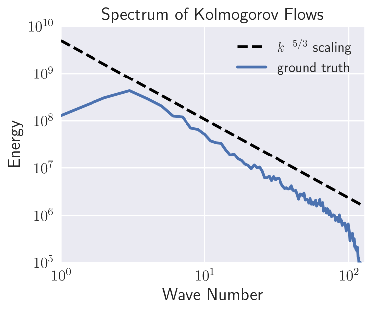
Figure 2: The spectrum of Kolmogorov flow decays exponentially with the Kolmogorov scale of $5/3$ in the inverse cascade range.

3.2 Low-frequency components in PDEs

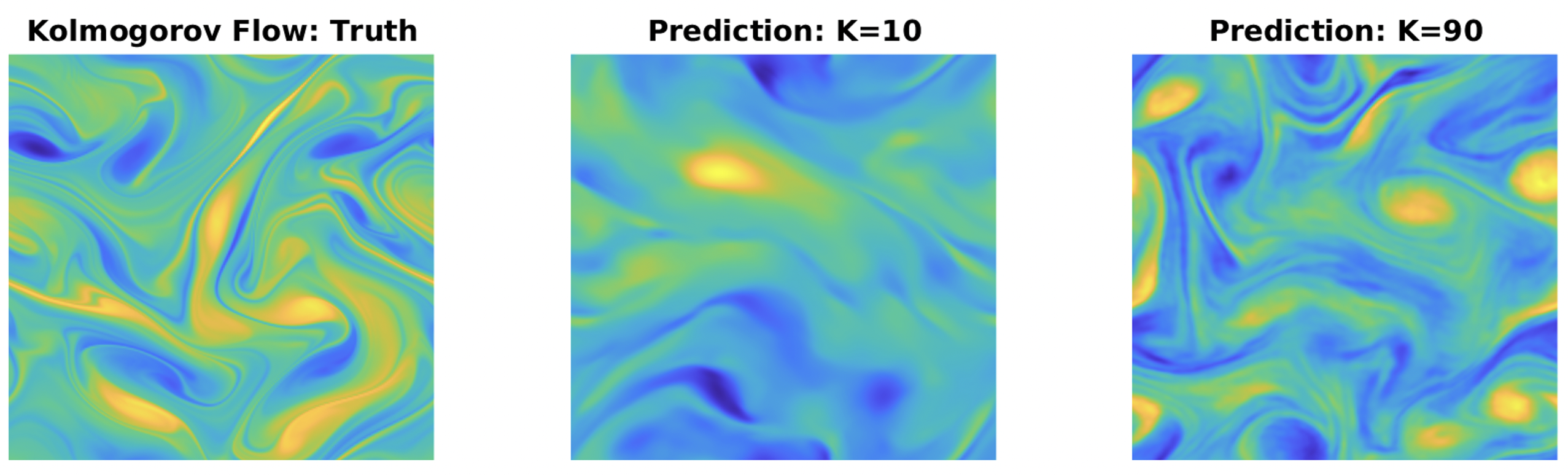
Figure 3: FNO with higher frequency modes captures smaller-scale structures in the turbulence. Prediction of the Kolmogorov flow by FNO with $K=10$ and $K=90$. Insufficient modes lead to overly strong dumping and it fails to capture small-scale structures in the turbulence of Kolmogorov flow.

Learning frequency modes is important as large-scale, low-frequency components usually have larger magnitudes than small-scale, high-frequency components in PDEs. For dissipative systems (with diffusion terms) such as the viscous Burgers’ equation and incompressible Navier-Stokes equation, the energy cascade involves the transfer of energy from large scales of motion to the small scales, which leads to the Kolmogorov spectrum with the slope of $k^{-5/3}$ in the inverse cascade range (Figure 2), and $k^{-3}$ in the direct-cascade range (Boffetta et al., 2012). The smallest scales in turbulent flow is called the Kolmogorov microscales. Therefore, one should choose the model frequencies with respect to the underlying equation frequencies when designing machine learning models. It would be a challenge to select the correct model frequencies in advance, without knowing the properties of the underlying PDEs.

4 Difficulties in Training Fourier Neural Operators

Although FNO has shown impressive performance in solving PDEs, the training remains to be a challenge. In this section, we discuss the main difficulties in training FNO.

4.1 The selection of effective modes

While frequency truncation $T_{K}$ ensures the discretization-invariance property of FNO, it is still challenging to select an appropriate number of effective modes $K$, as it is task-dependent and requires careful hyperparameter tuning.

Inappropriate selection of $K$ can lead to severe performance degradation. Setting $K$ too small will result in too few frequency modes, such that it delivers sufficient information for learning the solution operator, resulting in underfitting. As shown in Figure 3, in the prediction of Kolmogorov flow, FNO requires higher frequency modes to capture small-scale structures in turbulence for better performance. On the other hand, a larger $K$ with too many effective frequency modes may encourage FNO to interpolate the noise in the high-frequency components, leading to overfitting.

Previously, people have to choose the number of effective modes in FNO by estimating the underlying data frequencies, or using heuristics borrowed from pseudospectral solvers such as the 2/3 dealiaising rule (Hou & Li, 2007), i.e., picking the max Fourier modes as 2/3 of the training data resolution. However, it’s usually not easy to estimate the underlying frequency and the resolution of data may vary during training and testing. These problems lead to hand-tuning or grid-searching the optimal effective modes, which can be expensive and wasteful.

4.2 Regularization in FNO training

As discussed in Section 3, learning low-frequency modes is important for the successful training of FNO. However, the standard regularization techniques used in training neural networks are not capable of explicitly promoting the learning of low-frequency modes.

As shown in Figure 4, although FNO with well-tuned weight decay strength successfully regularizes the high-frequency modes, its regularization can be too strong for certain layers (such as the fourth operator in the figure). This leads to the instability of the frequency evolution, which damages the generalization performance as shown in Table 1. On the other hand, insufficient decay strength is not able to regularize the high-frequency modes and can even lead to the overfitting of the associated high-frequency noise. We extend our discussion about it in the appendix.

Algorithm 1 IFNO algorithm for 1D problem.

  Input: initial number of effective modes $K_{0}$ and mode buffers $b$, threshold $\alpha$

  Initialize: randomly initialize $R_{0}\in\mathbb{C}^{(K_{0}+b)\times\textrm{C}\times\textrm{C}}$

  For iteration $t$ in $1,...,T$:

    compute $s_{t}$ = $[S_{1},S_{2},...,S_{K_{t-1}+b}]$ // compute the frequency strength for each mode

    $K_{t}\leftarrow K_{t-1}$

   While $g(s_{t},K_{t})<\alpha$: // find $K_{t}$ that explains at least $\alpha$ of $s_{t}$

     $K_{t}\leftarrow K_{t}+1$

    construct $R_{t}\in\mathbb{C}^{(K_{t}+b)\times\textrm{C}\times\textrm{C}}$ where $R_{t}[0:(K_{t-1}+b),:,:]=R_{t-1}$ and initialize the rest randomly

4.3 Computational cost in training large-scale FNO

When training FNO to solve complex PDEs that consist of important high-frequency information, the number of effective modes $K$ needs to be large to well capture the solution operator.

However, this requires constructing a large-scale transformation $R$, which dominates the computational cost of the entire operations in FNO. This makes the training and inference more computationally expensive. For example, the Forecastnet (Pathak et al., 2022) for global weather forecast based on FNO is trained on 64 NVIDIA^® Tesla^® A100 GPUs, only covering a few key variables. And to simulate all the weather variables, it potentially needs the parallel FNO which scales to 768 GPUs(Grady II et al., 2022).

5 IFNO - Incremental Fourier Neural Operator

To address the above challenges, we propose Incremental Fourier Neural Operator (IFNO). IFNO automatically adjusts the number of effective modes $K$ during training. It starts with a ”small” FNO model with limited low-frequency modes and gradually increases $K$ based on the training progress or frequency evolution.

One of the key challenges in training IFNO is determining an appropriate time to proceed with the increase of $K$. A common practice is to use the training progress as a proxy to determine the time, as seen in previous work such as Liu et al. . Specifically, we let the algorithm increases $K$ only if the training loss is decreased by less than a threshold $\epsilon$ for $N$ epochs. We denote it as the loss-based IFNO algorithm. Despite its simplicity, this heuristic has been shown to be effective in practice. However, finding an appropriate $\epsilon$ and $N$ is challenging as it depends on the specific problem and the loss function. To address this issue, we propose a novel method to determine the expanding time by directly considering the frequency evolution in the parameter space.

5.1 Determination based on frequency evolution

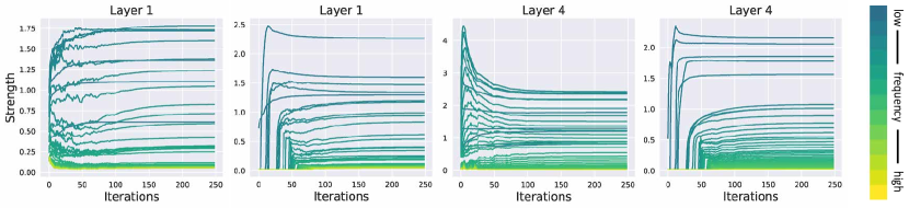
Figure 4: Frequency evolution of first and fourth Fourier convolution operators in FNO and IFNO during the training on Burgers’ equation. We visualize FNO on the left figure and IFNO on the right figure for each layer. Each frequency strength $S_{k}$ is visualized across training. FNO is tuned with the optimal weight decay strength.

As shown in Equation 1, $i$-th frequency strength $S_{i}$ reflects the importance of the $i$-th frequency mode in the model. The entire spectrum of the transformation $R$ can be represented by the collection of $p$ frequency strengths (when $p$ is sufficiently large):

$$s_{p}=[S_{1},S_{2},...,S_{p}],$$ (2)

where $s_{p}\in\mathbb{R}^{p}$.

When applying the frequency truncation $T_{K}$ ($K<p$), we can measure how much the lowest $K$ frequency modes explain the total spectrum by computing the explanation ratio $g(K,s_{p})$.

$$g(K,s_{p})=\frac{\sum_{k=1}^{K}S_{k}}{\sum_{k=1}^{p}S_{k}}.$$ (3)

We define a threshold $\alpha$, which is used to determine if the current modes can well explain the underlying spectrum. If $g(K,s_{p})>\alpha$, it indicates that the current modes are sufficient to capture the important information in the spectrum, and thus no additional modes need to be included in FNO. Otherwise, more frequency modes will be added into the model until $g(K,s_{p})>\alpha$ is satisfied.

Although $s_{p}$ reflects the entire spectrum when $p$ is sufficiently large, maintaining a large $p$ is unnecessary and computationally expensive. Instead, we only maintain a truncated spectrum $s_{K+b}\in\mathbb{R}^{K+b}$, which consists of $K$ effective modes and $b$ buffer modes. The buffer modes contain all mode candidacies that potentially would be included as effective modes in the later stage of training.

In practice, at iteration $t$ with $K_{t}$ effective modes, we construct a transformation $R_{t}\in\mathbb{C}^{(K_{t}+b)\times\textrm{C}\times\textrm{C}}$ for 1D problems. After updating $R_{t}$ at iteration $t+1$, we will find $K_{t+1}$ that satisfies $g(K_{t+1},s_{t})>\alpha$. In this way, we can gradually include more high-frequency modes when their evolution becomes more significant, as illustrated in Figure 1. We also describe how IFNO is trained for solving 1D problems in Algorithm 1.

IFNO is extremely efficient as the training only requires a part of frequency modes. In practice, it also converges to a model requiring fewer modes than the baseline FNO without losing any performance, making the model efficient for inference. Notably, the cost of computing the frequency strength and explanation ratio is negligible compared to the total training cost. It can be further reduced by performing the determination every $T$ iterations, which does not affect the performance.

Dynamic Spectral Regularization

As discussed in Section 4.2, learning low-frequency modes is important in FNO but standard regularization techniques (such as weight decay) do not have the ability to appropriately regularize the frequency evolution. However, we find that IFNO can be served as a dynamic spectral regularization process. As shown in Figure 4, IFNO properly regularizes the frequency evolution without causing any instability or overfitting high-frequency modes. As we will present in the experiment section, the dynamic spectral regularization gives IFNO a significant generalization improvement.

6 Evaluations

6.1 Experimental Setup

We evaluate IFNO and its variants on 4 different datasets of increasing difficulty. We retain the structure of the original FNO which consists of stacking four Fourier convolution operator layers with the ReLU activation as well as batch normalization. More specifically for the time-dependent problems we use an RNN structure in time that directly learns in space-time. For all the datasets, the initial and coefficient conditions are sampled from Gaussian random fields (Nelsen & Stuart, 2021).

Burgers’ Equation

We consider the 1D Burgers’ equation, which is a non-linear PDE with various applications, including modeling the flow of a viscous fluid. The 1D Burgers’ equation takes the form:

$$\partial_{t}u(x,t)+\partial_{x}\left(u^{2}(x,t)/2\right) =\nu\partial_{xx}u(x,t), t\in(0,1]$$

$$u(x,0) =u_{0}(x), x\in(0,1)$$

where $u_{0}$ is the initial condition and $\nu$ is the viscosity coefficient. We aim to learn the operator $\mathcal{G}_{\theta}$ mapping the initial condition to the solution. The training is performed under the resolution of 1024, and we consider the learning rate that is halved every 50 epochs and weight decay to be 0.0001.

Darcy Flow

Next, we consider the steady-state of the 2D Darcy Flow on the unit box, which is the second-order, linear, elliptic PDE:

$$-\nabla\cdot(a(x)\nabla u(x)) =f(x), x\in(0,1)^{2}$$

$$u(x) =0, x\in\partial(0,1)^{2}$$

with a Dirichlet boundary where $a$ is the diffusion coefficient and $f=1$ is the forcing function. We are interested in learning the operator mapping the diffusion coefficient to the solution. The resolution is set to be $421\times 421$ across all experiments.

Navier-Stokes Equation

Table 1: Evaluation on various PDEs in the few-data regime. The average training and testing L2 loss are reported with their standard deviation over 3 repeated runs. Frequency-based and loss-based IFNO are compared with standard FNO with fixed $K=10,30,60,90$ number of modes. Losses have been divided by the scale under the column.

Method	Burgers		Darcy Flow		Navier Stokes (FNO2D)
	Train ($110-3$)	Test ($110-1$)	Train ($110-3$)	Test (1e-5)	Train ($110-3$)	Test (1)
IFNO (Freq)	$0.310\pm 0.050$	0.874 $\pm$ 0.044	0.059 $\pm$ 0.001	1.127 $\pm$ 0.034	$142.3\pm 6.621$	0.589 $\pm$ 0.017
IFNO (Loss)	$13.53\pm 13.08$	$1.197\pm 0.398$	0.059 $\pm$ 0.001	$1.128\pm 0.025$	$126.8\pm 17.51$	$0.616\pm 0.017$
FNO (10)	$2.844\pm 0.070$	$0.934\pm 0.054$	0.061 $\pm$ 0.001	$1.144\pm 0.020$	$139.9\pm 6.913$	$0.618\pm 0.004$
FNO (30)	$0.276\pm 0.083$	$0.960\pm 0.004$	0.060 $\pm$ 0.003	$1.123\pm 0.011$	$118.6\pm 11.58$	$0.638\pm 0.018$
FNO (60)	$0.316\pm 0.015$	$0.899\pm 0.028$	0.060 $\pm$ 0.002	$1.138\pm 0.005$	87.64 $\pm$ 8.016	$0.644\pm 0.013$
FNO (90)	0.158 $\pm$ 0.064	$0.896\pm 0.022$	0.059 $\pm$ 0.001	$1.130\pm 0.023$	$113.7\pm 12.12$	$0.645\pm 0.022$

Method	Navier Stokes (FNO3D)		Kolmogorov Flow
	Train ($110-3$)	Test ($110-1$)	Train ($110-3$)	Test ($110-1$)
IFNO (Freq)	$4.350\pm 0.194$	$5.575\pm 0.039$	36.25 $\pm$ 0.533	$1.290\pm 0.022$
IFNO (Loss)	$2.083\pm 0.277$	$5.605\pm 0.051$	34.44 $\pm$ 1.075	1.275 $\pm$ 0.015
FNO (10)	$5.393\pm 0.070$	5.570 $\pm$ 0.014	142.3 $\pm$ 0.432	$1.792\pm 0.003$
FNO (30)	1.895 $\pm$ 0.273	$5.627\pm 0.073$	69.91 $\pm$ 0.511	$1.392\pm 0.022$
FNO (60)	$-$	$-$	38.59 $\pm$ 0.333	$1.386\pm 0.023$
FNO (90)	$-$	$-$	29.05 $\pm$ 1.066	$1.387\pm 0.015$

We also consider the 2D+time Navier-Stokes equation for a viscous, incompressible fluid on the unit torus:

$$\partial_{t}w(x,t)+u(x,t)\cdot\nabla w(x,t) =\nu\Delta w(x,t)+f(x),$$

$$\nabla\cdot u(x,t) =0,\;\;x\in(0,1)^{2}$$

$$w(x,0) =w_{0}(x),\;\;t\in(0,T]$$

where $w=\nabla\times u$ is the vorticity, $w_{0}$ is the initial vorticity, $\nu\in\mathbb{R}_{+}$is the viscosity coefficient, and $f(x)=0.1\bigl{(}\mathrm{sin}(2\pi(x_{1}+x_{2}))+\mathrm{cos}(2\pi(x_{1}+x_{2}))\bigr{)}$ is the forcing function. We are interested in learning the operator mapping the vorticity up to time 10 to the vorticity up to some later time. We experiment with the hardest viscosity task i.e $\nu=1\mathrm{e}-5$. The equivalent Reynolds number is around $500$ normalized by forcing and domain size. We set the final time $T=20$ as the dynamic becomes chaotic. The resolution is fixed to be $64\times 64$.

We consider solving this equation using the 2D FNO with an RNN structure in time or using the 3D FNO to do space-time convolution, similar to the benchmark in Li et al. (a). As 3D FNO requires significantly more parameters, evaluating 3D FNO with more than 30 modes is computationally intractable due to the hardware limitation.

Kolmogorov Flow

At last, we evaluate the models on high-frequency Kolmogorov Flow with Reynolds number 500. It is governed by the 2D Navier-Stokes equation, with forcing $f(x)=\mathrm{sin}(nx_{2})\hat{x}_{1}$, where $x_{1}$ is the unit vector and a larger domain size $[0,2\pi]$, as studied in (Li et al., 2021; Kochkov et al., 2021). We consider learning the evolution operator from the previous time step to the next based on 2D FNO. The resolution is fixed to be $256\times 256$ to show high frequency details. Notably, this is a much more challenging problem compared to the previous datasets.

Methods

We present our results for each dataset where we consider 4 standard FNO baselines with different numbers of frequency modes $K=10,30,60,90$. We denote FNO (Freq) as our mainly proposed algorithm that determines the mode increase based on the frequency evolution, as described in Algorithm 1. We also consider the simple variant that increases the frequency modes based on the training progress (training loss), which we denote as FNO (Loss). For each dataset, all methods are trained with the same hyperparameters, including the learning rate, weight decay, and the number of epochs. Unless otherwise specified, we use the Adam optimizer to train for 500 epochs with an initial learning rate of 0.001 that is halved every 100 epochs and weight decay set to be 0.0005. All experiments are run using NVIDIA^® Tesla^® V100 GPUs, and we repeat each experiment with 3 different random seeds.

6.2 Hyperparameter settings

We find IFNO is less sensitive to hyperparameters across different datasets. We use the same hyperparameters for all datasets, including the number of initial modes $K_{0}=1$, the number of buffer modes $b=5$, and the threshold $\alpha=0.99$. We also use an uniform threshold $\epsilon=0.001$ to determine whether the training progress is stalled in IFNO (Loss).

Insensitivity to hyperparameters is a nice property for IFNO, as it allows us to adopt FNO architecture to a wide range of problems without expensive trial-and-error experiments for finding an appropriate $K$.

6.3 Results

We evaluate all methods in the few-data regime across different datasets. The few-data regime means that the models only have the access to very limited data samples. This is a common scenario in many real-world PDE problems where accurately labeled data is expensive to obtain. In this regime, the ability to generalize well is highly desirable. We consider a small training set (5 to 50 samples) for Burgers, Darcy, and Navier-Stokes datasets. As the data trajectories are already limited in Kolmogorov dataset, we choose 8x larger time step (sampling rate ) for each trajectory, resulting in fewer time frames.

As shown in Table 1, IFNO (Freq) consistently outperforms the FNO baselines across all datasets, regardless of the number of modes $K$. It also shows that FNO with larger $K$ achieves lower training loss, but it overfits the training data and performs poorly on the testing set. On the other hand, IFNO (Freq) achieves slightly higher training loss but generalizes well to the testing set, which demonstrates the effectiveness of the dynamic spectral regularization. We also notice that although IFNO (Loss) has significant fluctuations especially in the training results, it does achieve better generalization on most datasets against the baselines.

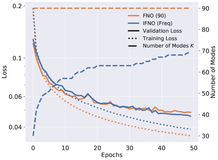
Figure 5: Testing loss, training loss, and number of modes $K$ during the training of FNO and IFNO on Kolmogorov flow.

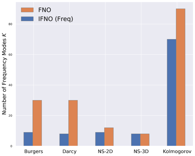
Figure 6: Number of frequency modes $K$ in the converged FNO and IFNO models across datasets. We report $K$ in the first Fourier convolution operator. NS denotes Navier-Stokes equations.

Figure 5 compares FNO (90) and IFNO (Freq) over the training on Kolmogorov flow. It shows that IFNO requires much fewer frequency modes during training. As the linear transformation $R$ dominates the number of parameters and FLOPs in FNO when $K$ is large, IFNO (Freq) can significantly reduce the computational cost and memory usage of training FNO.

IFNO not only achieves better generalization but even requires fewer modes at the end of training. In Figure 6, we compare IFNO (Freq) with FNO with a particular $K$ that achieves the best performance in each dataset. The results suggest that the trained IFNO (Freq) consistently requires fewer frequency modes than its FNO counterpart, which makes the inference of IFNO more efficient. This also indicates that IFNO can automatically determine the optimal number of frequency modes $K$ during training, without predetermine $K$ as an inductive bias that could potentially hurt the performance.

7 Related Works

The applications of neural networks on partial differential equations have a long history(Lagaris et al., 1998; Dissanayake & Phan-Thien, 1994). These deep learning methods can be classified into three categories: (1) ML-enhanced numerical solvers such as learned finite element, finite difference, and multigrid solvers (Kochkov et al., 2021; Pathak et al., 2021; Greenfeld et al., 2019) ; (2) Network network-based solvers such as Physics-Informed Neural Networks (PINNs), Deep Galerkin Method, and Deep Ritz Method (Raissi et al., 2019; Sirignano & Spiliopoulos, 2018; Weinan & Yu, 2018); and (3) the data-driven surrogate models such as (Guo et al., 2016; Zhu & Zabaras, 2018; Bhatnagar et al., 2019). Among them, the machine learning surrogate models directly parameterized the target mapping based on the dataset. They do not require a priori knowledge of the governing system, and they usually enjoy a light-fast inference speed. Recently a novel class of surrogate models called neural operators is developed (Li et al., b; Lu et al., 2021; Kissas et al., 2022). Neural operators parameterize the PDEs’ solution operator in the function spaces and leverage its mathematical structures in their architectures. Consequentially, neural operators usually have a better empirical performance (Takamoto et al., 2022) and theoretical guarantees (Kovachki et al., 2021) combined with conventional deep learning models.

The concept of implicit spectral bias was first proposed by Rahaman et al. as a possible explanation for the generalization capabilities of deep neural networks. There have been various results towards theoretically understanding this phenomenon (Cao et al., ; Basri et al., ). Fridovich-Keil et al. further propose methodologies to measure the implicit spectral bias on practical image classification tasks. Despite a wealth of theoretical results and empirical observations, there has been no prior research connecting the implicit spectral bias with FNO to explain its good generalization across different resolutions.

The notion of incremental learning has been applied to the training of PINNs in the previous studies (Krishnapriyan et al., 2021; Huang & Alkhalifah, ). These works propose to train PINNs while incrementally increasing the complexity of the underlying PDE problem, such as training them on low-frequency wavefields first and on high-frequency ones later(Huang & Alkhalifah, ). However, our work is orthogonal to the previous methods as we study on incrementally expanding the model architectures under a fixed PDE problem. We leave it as a future work to apply IFNO under the curriculum learning paradigm to address optimization challenges.

8 Conclusion

In this work, we propose Incremental Fourier Neural Operator (IFNO) that incrementally selects frequency modes during training. Our results suggest that IFNO achieves better generalization while requiring less number of parameters (frequency modes) compared to the standard FNO. We believe IFNO opens many new possibilities, such as solving PDEs with limited labeled data and training computationally efficient neural operators. In the future, we plan to evaluate IFNO on more complex PDEs and extend it to other changeling settings, such as training physics-informed neural operators.

Appendix A Standard Regularization in training FNO

In the section, we visualize the frequency evolution of FNO and IFNO. As shown in Figure 7, the weight decay used in the optimization has a significant effect on the learned weights. When the weight decay is active, the strength of weights will converge around the first 100 iterations of training. Further, the strength of frequencies is ordered with respect to the wave numbers where the lower frequencies have high strength and the higher frequencies have lower strength. On the other hand, when training without weight decay, the strength of all frequency modes will continuously grow and mix up with each other.

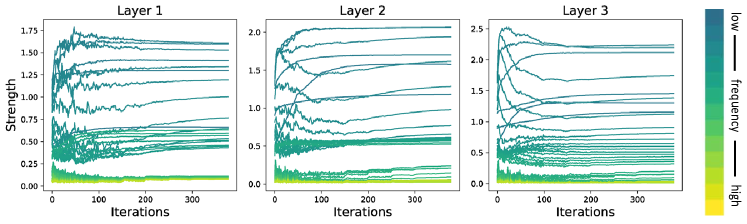
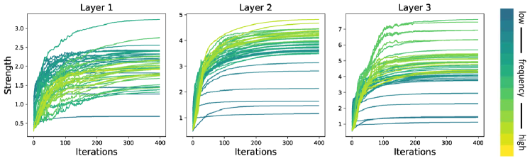
Figure 7: Frequency evolution of the Fourier convolution operators in FNO with and without weight decay. Top: with weight decay; bottom: without weight decay. When training with weight decay, the strength of each mode converges around 100 training iterations. And the weights of lower frequency tend to have high strength. On the other hand, the weight continues growing throughout the training without the weight decay. In this case, higher frequencies can also have high strength.

Appendix B Additional Results

B.1 Full Data Results

We evaluate the models with the most data samples available in each dataset. As shown in Table 2, IFNO achieves good performance comparable with standard FNO. It even achieves the best testing performance on Navier Stokes (2D) and Kolmogorov Flow.

Table 2: Evaluation on various PDEs in the full data regime. The average training and testing L2 loss are reported with their standard deviation over 3 repeated runs. Frequency-based and loss-based IFNO are compared with standard FNO with fixed $K=10,30,60,90$ number of modes. Losses have been divided by the scale under the column.

Method	Burgers		Darcy Flow		Navier Stokes (FNO 2D)
	Train ($110-3$)	Test ($110-3$)	Train ($110-4$)	Test (1e-4)	Train ($110-1$)	Test (1e-1)
IFNO (Freq)	$0.432\pm 0.018$	0.546 $\pm$ 0.020	0.447 $\pm$ 0.006	0.509 $\pm$ 0.020	$1.383\pm 0.015$	1.905 $\pm$ 0.017
IFNO (Loss)	$0.391\pm 0.027$	$0.595\pm 0.105$	0.405 $\pm$ 0.034	$0.464\pm 0.048$	1.325 $\pm$ 0.003	$1.918\pm 0.006$
FNO (10)	$0.441\pm 0.015$	$0.576\pm 0.006$	0.422 $\pm$ 0.012	$0.479\pm 0.019$	$1.409\pm 0.006$	$1.912\pm 0.021$
FNO (30)	0.382 $\pm$ 0.008	0.499 $\pm$ 0.003	0.390 $\pm$ 0.024	0.449 $\pm$ 0.026	$1.346\pm 0.011$	$1.934\pm 0.012$
FNO (60)	$0.385\pm 0.017$	$0.518\pm 0.004$	0.433 $\pm$ 0.015	$0.485\pm 0.020$	1.350 $\pm$ 0.011	$1.931\pm 0.012$
FNO (90)	0.394 $\pm$ 0.011	$0.540\pm 0.039$	0.424 $\pm$ 0.006	$0.489\pm 0.030$	$1.335\pm 0.012$	$1.927\pm 0.006$

Method	Navier Stokes (FNO 3D)		Kolmogorov Flow
	Train ($110-2$)	Test ($110-1$)	Train ($110-2$)	Test ($110-2$)
IFNO (Freq)	$4.843\pm 0.116$	$4.855\pm 0.005$	3.271 $\pm$ 0.025	4.343 $\pm$ 0.033
IFNO (Loss)	$2.798\pm 0.106$	$4.879\pm 0.013$	3.219 $\pm$ 0.139	5.032 $\pm$ 0.301
FNO (10)	$5.596\pm 0.030$	4.813 $\pm$ 0.013	12.26 $\pm$ 0.057	$13.28\pm 0.015$
FNO (30)	2.776 $\pm$ 0.098	$4.877\pm 0.008$	5.941 $\pm$ 0.023	$6.775\pm 0.019$
FNO (60)	$-$	$-$	3.789 $\pm$ 0.022	$4.865\pm 0.030$
FNO (90)	$-$	$-$	3.091 $\pm$ 0.022	$4.597\pm 0.070$

B.2 Frequency mode evolution during training

As shown in Figure 8, the effective modes $K$ adaptively increase during the training phase on the Burgers, Darcy, Navier-Stokes (2D & 3D formulation), and Kolmogorov Flows. For smooth problems such as viscous Burgers equation and Darcy Flow, the mode converges in the early epoch, while for problem with high frequency structures such as the Kolmogorov Flows, the mode will continuously increase throughout the training phase.

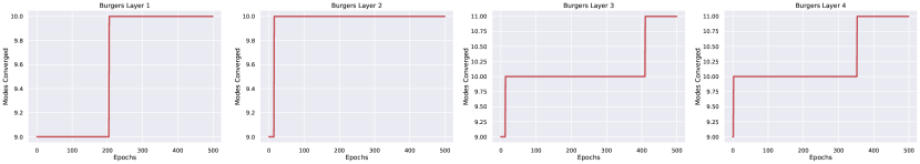
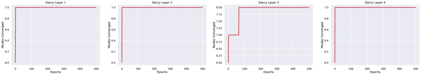
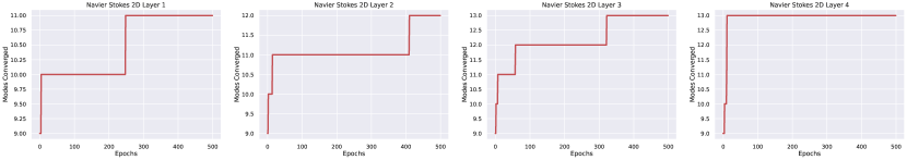
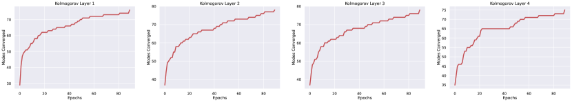
Figure 8: Mode evolution during training for each layer across datasets.

B.3 Training and testing loss during learning

Figure 9 and 10 show the training curves and testing curves across the five problem settings, ten rows in total. Overall, IFNO methods have a slightly higher training error but lower validation error, indicating its better generalization over the few data regime.

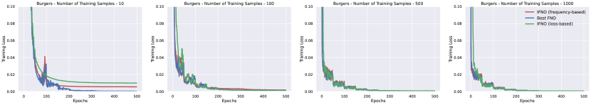
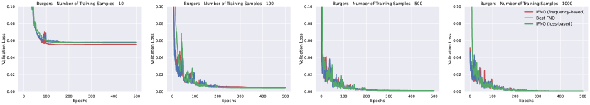
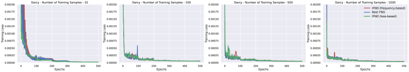
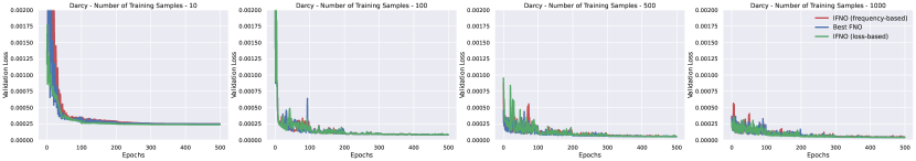
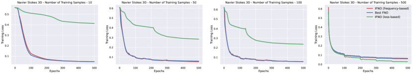
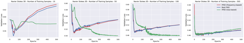
Figure 9: Loss vs Epochs across datasets (part 1: Burgers, Darcy, Navier-Stokes 2D). Each top row: training L2 loss. Each bottom row: validation L2 loss

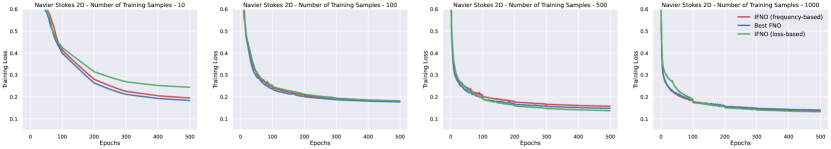
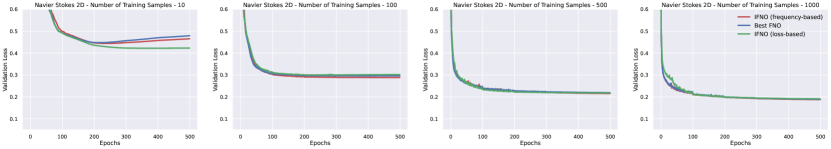
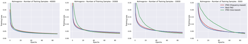
Figure 10: Loss vs Epochs across datasets (part 2: Navier-Stokes 2D, Kolmogorov Flows). Each top row: training L2 loss. Each bottom row: validation L2 loss

References

- (1) Basri, R., Jacobs, D., Kasten, Y., and Kritchman, S. The convergence rate of neural networks for learned functions of different frequencies. URL http://arxiv.org/abs/1906.00425. type: article.
- Bhatnagar et al. (2019) Bhatnagar, S., Afshar, Y., Pan, S., Duraisamy, K., and Kaushik, S. Prediction of aerodynamic flow fields using convolutional neural networks. Computational Mechanics, 64(2):525–545, 2019.
- Boffetta et al. (2012) Boffetta, G., Ecke, R. E., et al. Two-dimensional turbulence. Annual review of fluid mechanics, 44(1):427–451, 2012.
- (4) Cao, Y., Fang, Z., Wu, Y., Zhou, D.-X., and Gu, Q. Towards understanding the spectral bias of deep learning. URL http://arxiv.org/abs/1912.01198. type: article.
- Degrave et al. (2022) Degrave, J., Felici, F., Buchli, J., Neunert, M., Tracey, B., Carpanese, F., Ewalds, T., Hafner, R., Abdolmaleki, A., de Las Casas, D., et al. Magnetic control of tokamak plasmas through deep reinforcement learning. Nature, 602(7897):414–419, 2022.
- Dissanayake & Phan-Thien (1994) Dissanayake, M. and Phan-Thien, N. Neural-network-based approximations for solving partial differential equations. communications in Numerical Methods in Engineering, 10(3):195–201, 1994.
- (7) Fridovich-Keil, S., Gontijo-Lopes, R., and Roelofs, R. Spectral bias in practice: The role of function frequency in generalization. URL http://arxiv.org/abs/2110.02424. type: article.
- Gerfo et al. (2008) Gerfo, L. L., Rosasco, L., Odone, F., Vito, E. D., and Verri, A. Spectral Algorithms for Supervised Learning. Neural Computation, 20(7):1873–1897, 07 2008. ISSN 0899-7667. doi: 10.1162/neco.2008.05-07-517. URL https://doi.org/10.1162/neco.2008.05-07-517.
- Grady II et al. (2022) Grady II, T. J., Khan, R., Louboutin, M., Yin, Z., Witte, P. A., Chandra, R., Hewett, R. J., and Herrmann, F. J. Towards large-scale learned solvers for parametric pdes with model-parallel fourier neural operators. arXiv preprint arXiv:2204.01205, 2022.
- Greenfeld et al. (2019) Greenfeld, D., Galun, M., Basri, R., Yavneh, I., and Kimmel, R. Learning to optimize multigrid pde solvers. In International Conference on Machine Learning, pp. 2415–2423. PMLR, 2019.
- Guo et al. (2016) Guo, X., Li, W., and Iorio, F. Convolutional neural networks for steady flow approximation. In Proceedings of the 22nd ACM SIGKDD international conference on knowledge discovery and data mining, pp. 481–490, 2016.
- Hou & Li (2007) Hou, T. Y. and Li, R. Computing nearly singular solutions using pseudo-spectral methods. Journal of Computational Physics, 226(1):379–397, 2007.
- (13) Huang, X. and Alkhalifah, T. PINNup: Robust neural network wavefield solutions using frequency upscaling and neuron splitting. URL http://arxiv.org/abs/2109.14536.
- Jumper et al. (2021) Jumper, J., Evans, R., Pritzel, A., Green, T., Figurnov, M., Ronneberger, O., Tunyasuvunakool, K., Bates, R., Žídek, A., Potapenko, A., et al. Highly accurate protein structure prediction with alphafold. Nature, 596(7873):583–589, 2021.
- Kissas et al. (2022) Kissas, G., Seidman, J. H., Guilhoto, L. F., Preciado, V. M., Pappas, G. J., and Perdikaris, P. Learning operators with coupled attention. Journal of Machine Learning Research, 23(215):1–63, 2022.
- Kochkov et al. (2021) Kochkov, D., Smith, J. A., Alieva, A., Wang, Q., Brenner, M. P., and Hoyer, S. Machine learning accelerated computational fluid dynamics. arXiv preprint arXiv:2102.01010, 2021.
- Kovachki et al. (2021) Kovachki, N., Li, Z., Liu, B., Azizzadenesheli, K., Bhattacharya, K., Stuart, A., and Anandkumar, A. Neural operator: Learning maps between function spaces. arXiv preprint arXiv:2108.08481, 2021.
- Krishnapriyan et al. (2021) Krishnapriyan, A., Gholami, A., Zhe, S., Kirby, R., and Mahoney, M. W. Characterizing possible failure modes in physics-informed neural networks. In Ranzato, M., Beygelzimer, A., Dauphin, Y., Liang, P., and Vaughan, J. W. (eds.), Advances in Neural Information Processing Systems, volume 34, pp. 26548–26560. Curran Associates, Inc., 2021. URL https://proceedings.neurips.cc/paper/2021/file/df438e5206f31600e6ae4af72f2725f1-Paper.pdf.
- Lagaris et al. (1998) Lagaris, I. E., Likas, A., and Fotiadis, D. I. Artificial neural networks for solving ordinary and partial differential equations. IEEE transactions on neural networks, 9(5):987–1000, 1998.
- Li et al. (a) Li, Z., Kovachki, N., Azizzadenesheli, K., Liu, B., Bhattacharya, K., Stuart, A., and Anandkumar, A. Fourier neural operator for parametric partial differential equations, a. URL http://arxiv.org/abs/2010.08895. type: article.
- Li et al. (b) Li, Z., Kovachki, N., Azizzadenesheli, K., Liu, B., Bhattacharya, K., Stuart, A., and Anandkumar, A. Neural operator: Graph kernel network for partial differential equations, b. URL http://arxiv.org/abs/2003.03485.
- Li et al. (2021) Li, Z., Kovachki, N., Azizzadenesheli, K., Liu, B., Bhattacharya, K., Stuart, A., and Anandkumar, A. Markov neural operators for learning chaotic systems. arXiv preprint arXiv:2106.06898, 2021.
- Liu et al. (2022) Liu, B., Kovachki, N., Li, Z., Azizzadenesheli, K., Anandkumar, A., Stuart, A. M., and Bhattacharya, K. A learning-based multiscale method and its application to inelastic impact problems. Journal of the Mechanics and Physics of Solids, 158:104668, 2022.
- (24) Liu, Q., Wu, L., and Wang, D. Splitting steepest descent for growing neural architectures. URL http://arxiv.org/abs/1910.02366.
- Lu et al. (2021) Lu, L., Jin, P., Pang, G., Zhang, Z., and Karniadakis, G. E. Learning nonlinear operators via deeponet based on the universal approximation theorem of operators. Nature Machine Intelligence, 3(3):218–229, 2021.
- Nelsen & Stuart (2021) Nelsen, N. H. and Stuart, A. M. The random feature model for input-output maps between banach spaces. SIAM Journal on Scientific Computing, 43(5):A3212–A3243, 2021.
- Pathak et al. (2021) Pathak, J., Mustafa, M., Kashinath, K., Motheau, E., Kurth, T., and Day, M. Ml-pde: A framework for a machine learning enhanced pde solver. Bulletin of the American Physical Society, 2021.
- Pathak et al. (2022) Pathak, J., Subramanian, S., Harrington, P., Raja, S., Chattopadhyay, A., Mardani, M., Kurth, T., Hall, D., Li, Z., Azizzadenesheli, K., et al. Fourcastnet: A global data-driven high-resolution weather model using adaptive fourier neural operators. arXiv preprint arXiv:2202.11214, 2022.
- (29) Rahaman, N., Baratin, A., Arpit, D., Draxler, F., Lin, M., Hamprecht, F. A., Bengio, Y., and Courville, A. On the spectral bias of neural networks. URL http://arxiv.org/abs/1806.08734. type: article.
- Raissi et al. (2019) Raissi, M., Perdikaris, P., and Karniadakis, G. E. Physics-informed neural networks: A deep learning framework for solving forward and inverse problems involving nonlinear partial differential equations. Journal of Computational Physics, 378:686–707, 2019.
- Sirignano & Spiliopoulos (2018) Sirignano, J. and Spiliopoulos, K. Dgm: A deep learning algorithm for solving partial differential equations. Journal of computational physics, 375:1339–1364, 2018.
- Takamoto et al. (2022) Takamoto, M., Praditia, T., Leiteritz, R., MacKinlay, D., Alesiani, F., Pflüger, D., and Niepert, M. Pdebench: An extensive benchmark for scientific machine learning. arXiv preprint arXiv:2210.07182, 2022.
- Weinan & Yu (2018) Weinan, E. and Yu, B. The deep ritz method: a deep learning-based numerical algorithm for solving variational problems. Communications in Mathematics and Statistics, 6(1):1–12, 2018.
- Wen et al. (2022) Wen, G., Li, Z., Azizzadenesheli, K., Anandkumar, A., and Benson, S. M. U-fno—an enhanced fourier neural operator-based deep-learning model for multiphase flow. Advances in Water Resources, 163:104180, 2022.
- Xu et al. (2019) Xu, Z.-Q. J., Zhang, Y., Luo, T., Xiao, Y., and Ma, Z. Frequency principle: Fourier analysis sheds light on deep neural networks. arXiv preprint arXiv:1901.06523, 2019.
- Zhu & Zabaras (2018) Zhu, Y. and Zabaras, N. Bayesian deep convolutional encoder–decoder networks for surrogate modeling and uncertainty quantification. Journal of Computational Physics, 366:415–447, 2018.
- Zvyagin et al. (2022) Zvyagin, M. T., Brace, A., Hippe, K., Deng, Y., Zhang, B., Bohorquez, C. O., Clyde, A., Kale, B., Perez-Rivera, D., Ma, H., et al. Genslms: Genome-scale language models reveal sars-cov-2 evolutionary dynamics. bioRxiv, 2022.