Heterogeneous Graph Learning for Multi-modal Medical Data Analysis

Abstract

Routine clinical visits of a patient produce not only image data, but also non-image data containing clinical information regarding the patient, i.e., medical data is multi-modal in nature. Such heterogeneous modalities offer different and complementary perspectives on the same patient, resulting in more accurate clinical decisions when they are properly combined. However, despite its significance, how to effectively fuse the multi-modal medical data into a unified framework has received relatively little attention. In this paper, we propose an effective graph-based framework called HetMed (Heterogeneous Graph Learning for Multi-modal Medical Data Analysis) for fusing the multi-modal medical data. Specifically, we construct a multiplex network that incorporates multiple types of non-image features of patients to capture the complex relationship between patients in a systematic way, which leads to more accurate clinical decisions. Extensive experiments on various real-world datasets demonstrate the superiority and practicality of HetMed. The source code for HetMed is available at https://github.com/Sein-Kim/Multimodal-Medical.

1 Introduction

Along with recent advances of deep convolutional neural networks (CNNs) in computer vision domain, analyzing medical image with CNNs have achieved great success in patient healthcare (Azizi et al. 2021; Sun, Yu, and Batmanghelich 2021; Taleb et al. 2020; Deng et al. 2020; Aggarwal et al. 2021). Despite their success, they pay little attention to the inherent uniqueness of medical data: medical data is multi-modal in nature. That is, routine clinical visits of a patient produce not only image data, but also non-image data containing clinical information regarding the patient (Cui et al. 2022), which offers complementary diagnostic information of patients. More precisely, image data includes images of various body parts used for diagnostic or treatment purposes, while non-image data includes clinical data (e.g., demographic features and diagnosis) and lab test results (e.g., structured genomic sequences and blood test results). Such heterogeneous medical data provides different and complementary views of the same patient, leading to more accurate clinical decisions when they are properly combined. Hence, it is crucial to study how to integrate the multi-modal medical data for medical image analysis, which is relatively under explored despite its importance.

However, effectively fusing the multi-modal medical data is not a trivial task since a variety of clinical modalities contain their own distinct information and may have different data format (Cui et al. 2022). Some studies reflect multiple modalities in an “early fusion” manner by combining images of different modalities (e.g., positron emission tomography (PET), computed tomography (CT) and magnetic resonance imaging (MRI)) before training the model (Teramoto et al. 2016; Tan et al. 2020; Guo et al. 2019). On the other hand, “late fusion” approaches combine representations of different imaging modalities (Liu et al. 2021; Suk et al. 2014; Xu et al. 2016), while others learn from both image and non-image medical data by combining information from independently trained models in a post-hoc manner (Sanyal, Kar, and Sarkar 2021; Akselrod-Ballin et al. 2019; Cheerla and Gevaert 2019). A recent approach proposes end-to-end learning strategies for fusing multi-modal features at different stages of the model training, i.e., fusing intermediate features and output probabilities (Holste et al. 2021). However, current practice of naively integrating different modalities cannot fully benefit from the complementary relationship between multiple modalities.

In this work, we focus on the fact that patients who share similar non-image data are likely to suffer from the same disease. For example, it is well known that a group of people possessing the E4 allele of apolipoprotein E (APOE) has the primary genetic risk factor for the sporadic form of Alzheimer’s Disease (AD) (Emrani et al. 2020). Hence, by introducing non-image data (e.g., APOE in the tabular data) in addition to image data, we argue that preemptive clinical decisions can be made at an early stage of AD, which may not be detected based on image data only.

To elaborate our argument, we compare the similarity of non-image data between various levels of dementia with OASIS-3 (LaMontagne et al. 2019) dataset in which patients in the dataset are divided into four classes according to the severity of dementia assessed using Clinical Dementia Rating (CDR) scale (Morris 1991): CDR 0 indicates normal cognitive function, CDR 0.5 indicates very mild impairment, CDR 1 indicates mild impairment, and CDR 2 indicates moderate dementia. We calculate the average pairwise cosine similarities of patients’ non-image features within a class and between different classes in Figure 1 (a). We observe that the patients in the same class (i.e., diagonal) share high similarity compared with those in different classes (i.e., off-diagonal), demonstrating that patients with similar non-image data are more likely to suffer from the same disease. Furthermore, we find out that diverse aspects of non-image data induce complex similarity relationships between patients as shown in Figure 1 (b) and (c), i.e., the similarity among patients between different classes varies according to which features are selected for calculating the similarity. As a concrete example, consider two patients each of whom suffers from dementia of CDR 1 and 2, respectively. Incorporating personal and family historical list of patients (i.e., Type 1 features) may fail to find connections between the patients of CDR 1 and 2 as shown in Figure 1 (b). However, if the similarity is calculated based on the patients’ cognitive abilities (i.e., Type 2 features), we observe that the similarity between patients that belong to CDR 1 and 2 is relatively high, which indicates that mild impairment (i.e., CDR 1) likely leads to moderate dementia (i.e., CDR 2). This implies that considering complex relationship between patients induced by various types of features helps to capture implicit relationships that can play a key role in making medical decisions.

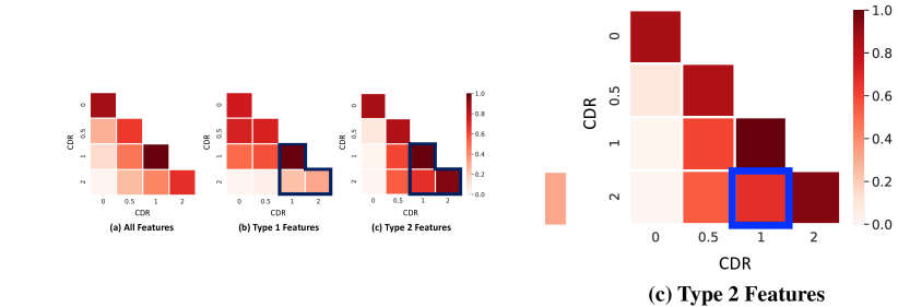
Figure 1: Average pairwise cosine similarity of patients’ non-image features between various CDR levels of dementia. Similarity is calculated with all features in (a), Type 1 features (i.e., personal and family historical list of patients) in (b), and Type 2 features (i.e., cognitive abilities reported by clinicians) in (c).

Contribution. In this work, we propose a general framework called HetMed (Heterogeneous Graph Learning for Multi-modal Medical Data Analysis) for fusing multi-modal medical data (i.e., image and non-image) based on a graph structure, which provides a natural way of representing patients and their similarities (Parisot et al. 2017). Specifically, each node in a graph denotes a patient associated with multi-modal features including medical images and non-image data of the patient. Moreover, each edge represents the similarity between patients in terms of non-image data. To capture the complex relationship between patients in a systematic way, we propose to construct a multiplex network (De Domenico et al. 2013) whose edges are connected according to the similarity of various feature combinations, revealing various types of relationship between patients. Our extensive experiments on various real-world datasets demonstrate the superiority of HetMed, showing that modeling complex relationships inherent between patients is crucial. A further appeal of integrating multi-modality into a graph structure, especially via a multiplex network, is that it shows robustness even with scarce label information.

2 Related Work

2.1 Medical Image Representation Learning

Training deep neural networks requires massive number of labeled data, which is time-consuming and expensive especially in medical domain. Recently, self-supervised representation learning methods for medical image has been recently proposed to alleviate the lack of training data. Inspired by SimCLR (Chen et al. 2020), Azizi et al. (2021) propose a loss function to maximize the mutual information between the images of the same patient. Sun, Yu, and Batmanghelich (2021) propose bi-level self-supervised learning objective for local anatomical level and patient-level. They use graph structure to model the relationship between different anatomical regions. For 3D medical images, Taleb et al. (2020) propose five self-supervised learning strategies inspired by recent computer vision approaches (Noroozi and Favaro 2016; Gidaris, Singh, and Komodakis 2018; Doersch, Gupta, and Efros 2015). Despite their success, they are designed to utilize only single-modality data, whereas multi-modal data are common in medical field.

2.2 Multi-modal Medical Image Analysis

By incorporating multiple modalities of medical data, machine learning models can trace patterns of diseases which cannot be captured by single modality of data. Some studies create multi-modal inputs to CNNs by combining images of multiple modalities (e.g., PET, CT and MRI) in an “early fusion” manner. Teramoto et al. (2016) identify initial pulmonary nodule candidates from both PET and CT images, and candidate regions from two images were combined for classification. Tan et al. (2020) propose medical image fusion method based on boundary measure modulated by a pulse-coupled neural network (Wang, Wang, and Guo 2018). Others learn from both image and non-image medical data by combining information from independently trained models in a post-hoc manner. Akselrod-Ballin et al. (2019) integrate XGBoost selected clinical features and mammography images to predict breast cancer of patients. Cheerla and Gevaert (2019) estimate the future course of patients with cancer lesions by fusing features that are independently learned from clinical data, mRNA expression data, microRNA expression data and histopathology whole slide images (WSIs). Recently, an end-to-end learning framework for fusing multiple modalities at different stages of model training has been proposed (Holste et al. 2021). However, a naive integration of the modalities cannot fully benefit from the complementary relationship between the modalities.

To address the issue, some recent works (Parisot et al. 2017; Kazi et al. 2019; Cao et al. 2021) suggest to fuse the multi-modalities into a graph structure. More precisely, each node feature is associated with a patient’s imaging feature vector, while edges represent the similarity between patients. These prior works, however, (a) do not consider inherent complex relationship between patients and (b) fail to show generalizability by only applying to a certain disease (e.g., autism spectrum disease and Alzheimer’s disease). Instead, we seek a general framework that encodes multi-modality into elaborately constructed network.

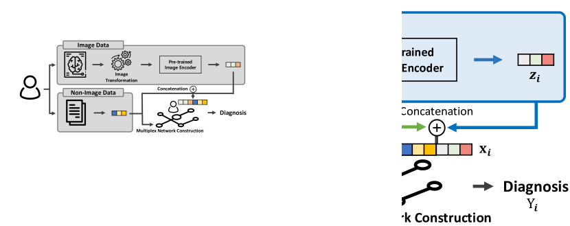
Figure 2: Overall model framework.

2.3 Multiplex Graph Neural Networks

With the recent success of deep neural networks, Graph Neural Networks (GNNs) extend the deep neural networks to deal with arbitrary graph-structured data. GNNs are trained by repeatedly aggregating the information from neighborhoods in a graph structure (Kipf and Welling 2016; Hamilton, Ying, and Leskovec 2017; Veličković et al. 2017; Lee et al. 2022a). Moreover, recent studies try to alleviate lack of label information with self-supervised learning methods (Zhu et al. 2020; Lee, Lee, and Park 2022; Lee et al. 2022b). However, by assuming only a single type of relationship between nodes, the above GNNs cannot deal with various types of edges which are prevalent in reality. A multiplex network, which is a type of heterogeneous graph (Shi et al. 2017), which is also known as multi-view graph (Qu et al. 2017), multi-layer graph (Li et al. 2018), multi-dimension graph (Ma et al. 2018), multi-relational graph (Schlichtkrull et al. 2018), and multiplex heterogeneous graph (Cen et al. 2019) in the literature, considers multiple types of relationships among a set of single-typed nodes. Recent multiplex network embedding methods aim to learn a single embedding for each node that captures multiple types of relationships associated with the node (Park et al. 2020; Jing, Park, and Tong 2021; Jing et al. 2021). MVE (Qu et al. 2017) and HAN (Wang et al. 2019) adopt attention approaches to combine embeddings learned from various relationships. DMGI (Park et al. 2020) and HDMI (Jing, Park, and Tong 2021) propose to adopt mutual information-based approaches to learn embeddings of nodes with consensus regularization and high order mutual information, respectively. To the best of our knowledge, this work is the first to employ a multiplex network to capture the complex relationship between patients for multi-modal medical image analysis.

3 Problem Statement

Definition 1. (Attributed Multiplex Network) An attributed multiplex network is a network $\mathcal{G}=\{\mathcal{G}^{(1)},...,\mathcal{G}^{(r)},...,\mathcal{G}^{(|\mathcal{R}|)}\}=\{\mathcal{V},\mathcal{E},\mathbf{X}\}$, where $\mathcal{G}^{(r)}=\{\mathcal{V},\mathcal{E}^{(r)},\mathbf{X}\}$ is a graph of the relation type $r\in\mathcal{R}$, $\mathcal{V}$ is the set of $n$ nodes, $\mathcal{E}=\bigcup_{r\in\mathcal{R}}{\mathcal{E}^{(r)}}\subseteq\mathcal{V}\times\mathcal{V}$ is the set of all edges with relation type $r$, and $\mathbf{X}\in\mathbb{R}^{|\mathcal{V}|\times F}$ is a matrix that encodes node attribute information for $n$ nodes. Given the network $\mathcal{G}$, $\mathcal{A}=\{\mathbf{A}^{(1)},...,\mathbf{A}^{(|\mathcal{R}|)}\}$ is a set of adjacency matrices, where $\mathbf{A}^{(r)}\in\{0,1\}^{|\mathcal{V}|\times|\mathcal{V}|}$ is an adjacency matrix of the network $\mathcal{G}^{(r)}$.

Task: Multi-modal Medical Image Analysis. Given a multi-modal medical data $\mathcal{D}=\{\mathbf{B},\mathbf{C},Y\}$, where $\mathbf{B}\in\mathbb{R}^{\mathcal{|V|}\times F_{\text{img}}}$ is the 2D or 3D medical image data, $\mathbf{C}\in\mathbb{R}^{\mathcal{|V|}\times F_{\text{non-img}}}$ is the non-image medical data that consists of categorical and numerical features, and $Y\in\mathbb{R}^{|\mathcal{V}|\times c}$ is the label matrix, where $c$ is the number of classes. The goal of multi-modal medical image analysis is to classify patient $i$ into label $Y_{i}$ given multi-modal medical data, i.e., medical image $\mathbf{b}_{i}\in\mathbf{B}\in\mathbb{R}^{\mathcal{|V|}\times F_{\text{img}}}$ and non-image data $\mathbf{c}_{i}\in\mathbf{C}\in\mathbb{R}^{\mathcal{|V|}\times F_{\text{non-img}}}$ of patient $i$.

4 Method

An overview of our proposed HetMed is shown in Fig. 2.

4.1 Image Preprocessing: Anatomical Standardized Image

Unlike ordinary images, medical images contain noisy information due to the difference in photographing devices and physical size variation per patient. To get medical image represented in standard anatomical information, we use a software called SimpleITK (Lowekamp et al. 2013; Yaniv et al. 2018) for medical image pre-processing that works as: $\mathbf{b}_{i}=\mathrm{T}_{opt}(\mathrm{T}_{s}(\mathrm{T}_{i}^{-1}(\mathbf{b}_{i}^{original}))$, transforming original image $\mathbf{b}_{i}^{original}$ of patient $i$ into preprocessed image $\mathbf{b}_{i}$ with standard anatomical coordinate. Transformation function $\mathrm{T}_{i}^{-1}$ is a fixed mapping function that maps patient $i$’s image domain to patient $i$’s virtual image domain, while $\mathrm{T}_{s}$ is a fixed mapping function that maps virtual image domain to standard anatomical image domain. Finally, $\mathrm{T}_{opt}$ is a modified mapping function for optimization. The transformation function, $\mathrm{T}_{i}^{-1}$ is a fixed mapping function which maps patient $i$’s image domain to patient $i$’s virtual image domain. $\mathrm{T}_{s}$ is fixed mapping function which maps virtual image domain to standard anatomical image domain. Finally, $\mathrm{T}_{opt}$ is modified mapping function for optimization.

4.2 Learning Medical Image Representation

After the image preprocessing step, we obtain representations of images through a pretrained image encoder. We adopt several previous self-supervised medical image representation learning methods to verify the generality of HetMed.

4.2.1. 2D Medical Image.

Following Azizi et al. (2021), we first pre-train an encoder network $f(\cdot):\mathbb{R}^{\mathcal{|V|}\times F_{\text{img}}}\rightarrow\mathbb{R}^{\mathcal{|V|}\times F_{z}}$ (i.e., a ResNet (He et al. 2016)) with non-medical image datasets (i.e., STL10 (Coates, Ng, and Lee 2011) and ImageNet (Deng et al. 2009)) by adopting recent self-supervised contrastive learning methods, e.g., SimCLR (Chen et al. 2020) and MoCo (He et al. 2020). After the non-medical image pre-training step, we adopt Multi-Instance Contrastive Learning (MICLe) loss (Azizi et al. 2021), which maximizes the mutual information between images from the same patient. More formally, given a randomly sampled mini-batch of patient $i$, two randomly selected medical images $\mathbf{b}_{i}^{1}$, $\mathbf{b}_{i}^{2}\in\mathbb{R}^{F_{\text{img}}}$ of patient $i$ are encoded via the encoder network $f(\cdot)$ to generate representations $\mathbf{z}_{i}^{1}$, $\mathbf{z}_{i}^{2}\in\mathbb{R}^{F_{\text{z}}}$, respectively. Given a mini-batch images of size $N$, the MICLe loss between patient $i$ and other patients is given as follows:

$$\mathcal{L}_{i}^{\mathrm{MICLe}}=-\log\frac{exp(sim(\mathbf{z}_{i}^{1},\mathbf{z}_{i}^{2})/\tau)}{\sum_{k=1}^{2N}\mathds{1}_{\left[k\neq i\right]}exp(sim(\mathbf{z}_{i},\mathbf{z}_{k})/\tau)}$$ (1)

where $sim(\cdot,\cdot)$ is the cosine similarity between two vectors, and $\tau$ is a temperature hyperparameter. Finally, the patient $i$’s image representation $\mathbf{z}_{i}$ is given by the mean of multiple images, i.e., $\mathbf{z}_{i}=1/K\sum_{k=1}^{K}{\mathbf{z}_{i}^{k}}$, where $\mathbf{z}_{i}^{k}$ is the representation of the $k$-th image of patient $i$, and $K$ is the number of images for a patient.

4.2.2. 3D Medical Image.

On the other hand, digital medical imaging systems can also create 3D images of human organs. With 3D images, medical staffs can access new angles, resolutions, and more details required for better medical decisions while minimizing radiation exposure of patients. However, inherent limited availability of 3D medical image data (Singh et al. 2020) makes it difficult to learn representations of 3D images by directly applying MICLe loss. Thus, we adopt recently proposed medical image representation learning approaches for 3D medical image, i.e. 3D Jigsaw, 3D Rotation and 3D Exampler (Taleb et al. 2020) to pre-train an encoder network $f(\cdot)$ that produces a medical image representation $\mathbf{z}_{i}\in\mathbb{R}^{F_{z}}$ for each patient $i$. These image representations are later used as node features of the multiplex network. Note that following (Taleb et al. 2020), we do not pre-train $f(\cdot)$ with non-medical image dataset.

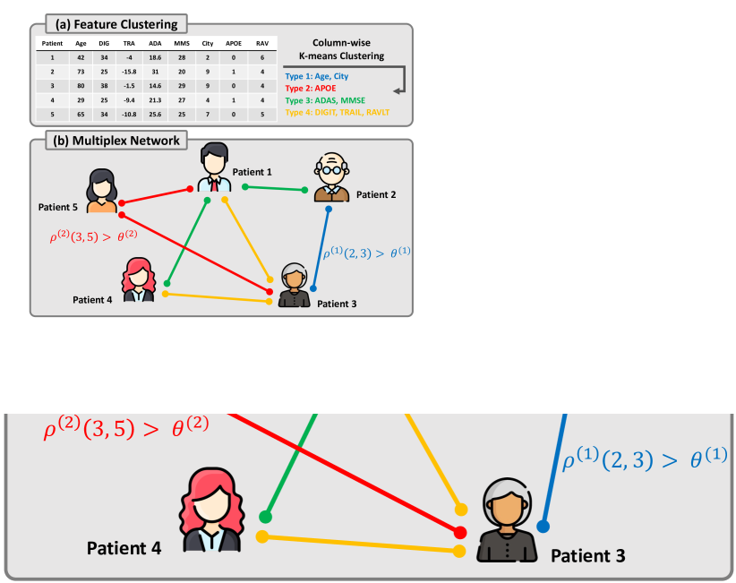
Figure 3: Multiplex network construction.

4.3 Multiplex Network Construction

In this section, we introduce how to construct a multiplex network to capture the inherent complex relationship between patients. Different from conventional approaches that utilize multiplex networks introduced in Section 2.3, where multiple types of relations are predefined (e.g., Paper-Author-Paper, Paper-Subject-Paper relationship in citation networks), relationship between patients are usually not given. Thus, the main challenge of constructing a multiplex network based on patient data is how to extract meaningful relationship between patients. On the other hand, non-image medical data contains various types of information regarding patients, e.g. demographic features, personal and family historical list and lab test results, each of which provides unique clinical information. That is, each type of non-image feature has a different connection to the target disease. For example, African Americans (i.e., demographic features) have been reported to have a higher prevalence of Alzheimer’s disease than Caucasians (Howell et al. 2017), while historical list (i.e., personal and family historical list) is an important non-modifiable risk factor for hypertension (Ranasinghe et al. 2015). Since non-image features can be categorized into several types regarding their characteristics, categorizing the features is the first step for relationship extraction.

Although adopting the domain knowledge is straightforward for the non-image features categorization, domain knowledge may (1) not be always available, and (2) not help discover implicit correlation between features. Thus, to automatically categorize various types of non-image features, we simply adopt K-means clustering algorithm  on the non-image tabular data $\mathbf{C}\in\mathbb{R}^{|\mathcal{V}|\times F_{\text{non-img}}}$ in a column-wise manner, which partitions the features in $F_{\text{non-img}}$ dimensions into $|\mathcal{R}|$ sets, i.e., $\mathbf{T}=\{T_{1},T_{2},\ldots,T_{|\mathcal{R}|}\}$. By doing so, we divide non-image data $\mathbf{C}$ into non-overlapping $|\mathcal{R}|$ types of features as shown in Figure 3 (a).

With $|\mathcal{R}|$ types of non-image features, we construct a multiplex network $\mathcal{G}=\{\mathcal{G}^{(1)},...,\mathcal{G}^{(r)},...,\mathcal{G}^{(|\mathcal{R}|)}\}$, where each $\mathcal{G}^{(r)}$ is constructed by calculating the cosine similarity of type $r$ features of non-image data, i.e., $\mathbf{C}^{(r)}$, as follows:

$$\centering\mathbf{A}^{(r)}(i,j)=\begin{cases}1&\mbox{if }\rho^{(r)}(i,j)>\theta^{(r)},\\ 0&\mbox{otherwise }\end{cases}\@add@centering$$ (2)

where $\rho^{(r)}(i,j)$ is the cosine similarity of type $r$ non-image feature between patient $i$ and $j$, i.e., $\rho^{(r)}(i,j)=\frac{\mathbf{c}^{(r)}_{i}\cdot\mathbf{c}^{(r)}_{j}}{\|\mathbf{c}^{(r)}_{i}\|\cdot\|\mathbf{c}^{(r)}_{j}\|}$ where $\mathbf{c}_{i}^{(r)}$ is the $i$-th row of $\mathbf{C}^{(r)}$, and $\theta^{(r)}$ is the threshold hyperparameter for each relation $r$. For example in Figure 3 (b), patient 2 and patient 3 are connected by relation type 1 since their age and city features (i.e. demographics type) are similar, while patient 3 and patient 5 are connected by APOE similarity (i.e., relation type 2). Finally, the image representation $\mathbf{Z}\in\mathbb{R}^{|\mathcal{V}|\times F_{z}}$, and non-image feature $\mathbf{C}\in\mathbb{R}^{|\mathcal{V}|\times F_{\text{non-img}}}$ are concatenated to generate the node attribute matrix $\mathbf{X}\in\mathbb{R}^{|\mathcal{V}|\times F}$ of multiplex network $\mathcal{G}$, i.e., $F=(F_{z}+F_{\text{non-img}})$.

4.4 Multiplex Graph Neural Networks

Given a multiplex network $\mathcal{G}$, learning from heterogeneous types of relationship among nodes is non-trivial, since these types of relationship are related (Park et al. 2020). Recently proposed multiplex network embedding methods captures interaction between relationships through attention mechanism (Wang et al. 2019) and consensus regularization (Park et al. 2020). Among various approaches for multiplex network embedding, we adopt DMGI (Park et al. 2020) in this work due to its simplicity and applicability under unsupervised setting. However, as HetMed is model-agnostic, any multiplex network embedding method can be adopted as will be demonstrated in Appendix 7.5.

Deep Multiplex Graph Infomax (DMGI). The core idea of DMGI is to learn the consensus embedding of a single node regarding multiple relation types, while each relation-type specific node embedding is trained to maximize the mutual information with relation-type specific summary vector. Specifically, relation-type specific node encoder $g_{r}(\cdot):\mathbb{R}^{|\mathcal{V}|\times F}\times\mathbb{R}^{|\mathcal{V}|\times|\mathcal{V}|}\rightarrow\mathbb{R}^{|\mathcal{V}|\times d}$ generates the relation-type specific node embedding matrix $\mathbf{H}^{(r)}\in\mathbb{R}^{|\mathcal{V}|\times d}$ for each relation type $r\in\mathcal{R}$. Then, the summary representation $\mathbf{s}^{(r)}$ of graph $\mathcal{G}^{(r)}$ is computed through mean pooling readout function. Given the embedding $\mathbf{H}^{(r)}$ and the summary vector $\mathbf{s}^{(r)}\in\mathbb{R}^{d}$, DMGI maximizes the mutual information between $\mathbf{H}^{(r)}$ and $\mathbf{s}^{(r)}$, while minimizing the mutual information between corrupted representation $\tilde{\mathbf{H}}^{(r)}$ and $\mathbf{s}^{(r)}$ as

$$\mathcal{L}^{(r)}=\sum_{i=1}^{\mathcal{|V|}}\log{\mathcal{D}(\mathbf{h}_{i}^{(r)},\mathbf{s}^{(r)})}+\sum_{j=1}^{\mathcal{|V|}}\log{(1-\mathcal{D}(\tilde{\mathbf{h}}_{j}^{(r)},\mathbf{s}^{(r)}))}$$ (3)

where $\mathcal{D}$ is a discrimination function that scores patch-summary representation pairs, i.e., high score for positive patch-summary pairs $(\mathbf{h}_{i}^{(r)},\mathbf{s}^{(r)})$, where $\mathbf{h}_{i}^{(r)}$ is the type $r$ embedding of node $v_{i}$. However, independently trained encoder $g_{r}(\cdot)$, which contains relevant information regarding each relation type $r$, cannot fully benefit from the multiplexity of the network. To this end, DMGI proposes consensus regularization which aims to minimize the discrepancy between relation specific embeddings, i.e., $\{\mathbf{H}^{(r)}|r\in\mathcal{R}\}$, and the consensus embedding $\mathbf{O}\in\mathbb{R}^{|V|\times d}$ as:

$$\ell_{cs}=\left[\mathbf{O}-\mathcal{Q}\left(\{\mathbf{H}^{(r)}|r\in\mathcal{R}\}\right)\right]^{2}-\left[\mathbf{O}-\mathcal{Q}\left(\{\tilde{\mathbf{H}}^{(r)}|r\in\mathcal{R}\}\right)\right]^{2}$$ (4)

where $\mathcal{Q}$ is an attentive pooling function for every relation-specific embedding matrix $\mathbf{H}^{(r)}$. Finally, we introduce a semi-supervised module to learn from labeled medical images based on the consensus embedding $\mathbf{O}$ as:

$$\ell_{sup}=-\frac{1}{|\mathcal{Y}_{L}|}\sum_{l\in\mathcal{Y}_{L}}{\sum_{i=1}^{c}{Y_{li}\ln{\hat{Y}_{li}}}}$$ (5)

where $\mathcal{Y}_{L}$ is the set of labeled node indices, $Y\in\mathbb{R}^{|\mathcal{V}|\times c}$ is the label matrix, and $\hat{Y}$ is the model prediction after passing the consensus embedding $\mathbf{O}$ through a softmax layer. Finally, our model is optimized to minimize the following loss:

$$\mathcal{L}=\sum_{r\in\mathcal{R}}{\mathcal{L}^{(r)}}+\alpha\ell_{cs}+\beta\ell_{sup}+\gamma\begin{Vmatrix}\boldsymbol{\Theta}\end{Vmatrix}^{2}$$ (6)

where $\alpha$, $\beta$, $\gamma$ are adjustable hyperparameters for each loss term, and $\boldsymbol{\Theta}$ is the trainable parameters of our model.

5 Experiments

5.1 Experimental Setup

Datasets. To evaluate our proposed HetMed, we conduct experiments on five multi-modal medical datasets. Specifically, we use three brain related datasets, and two breast-related datasets. Note that since 3D images can be readily converted to 2D images through slicing, we also report the performance on 3D image datasets when they are converted to 2D. The detailed statistics are summarized in Table 1 and further details on each dataset are described in Appendix 7.1.

Dataset	Body	Target	3D	# Non-Img	# Subjects	# Classes
	Parts	Disease		Features
ADNI	Brain	Alzheimer	✓	17	417	3
OASIS-3	Brain	Alzheimer	✓	19	979	4
ABIDE	Brain	Autism	✓	14	977	2
Duke-Breast	Breast	Tumor	✗	25	614	3
CMMD	Breast	Tumor	✗	4	1774	2

Table 1: Data statistics.

Model	ADNI		OASIS-3		ABIDE		Duke-Breast		CMMD
	Ma-F1	Mi-F1	Ma-F1	Mi-F1	Ma-F1	Mi-F1	Ma-F1	Mi-F1	Ma-F1	Mi-F1
Feat. (=MLP)	0.521	0.562	0.216	0.625	0.407	0.753	0.466	0.712	0.667	0.75
	(0.017)	(0.020)	(0.008)	(0.022)	(0.015)	(0.020)	(0.031)	(0.032)	(0.021)	(0.017)
Prob.	0.509	0.522	0.230	0.639	0.385	0.761	0.407	0.688	0.564	0.665
	(0.009)	(0.020)	(0.022)	(0.025)	(0.034)	(0.031)	(0.028)	(0.025)	(0.013)	(0.026)
Learned	0.576	0.598	0.199	0.647	0.649	0.776	0.484	0.625	0.714	0.773
	(0.012)	(0.022)	(0.009)	(0.010)	(0.021)	(0.023)	(0.022)	(0.024)	(0.032)	(0.020)
Spec.	0.628	0.788	0.202	0.679	0.696	0.717	0.427	0.701	0.681	0.742
	(0.009)	(0.018)	(0.011)	(0.014)	(0.032)	(0.037)	(0.010)	(0.025)	(0.036)	(0.024)
GCN	0.606	0.795	0.201	0.670	0.768	0.770	0.430	0.671	0.683	0.745
	(0.022)	(0.015)	(0.021)	(0.033)	(0.019)	(0.017)	(0.016)	(0.020)	(0.028)	(0.016)
HetMed	0.774	0.813	0.205	0.697	0.778	0.784	0.432	0.794	0.716	0.785
	(0.037)	(0.024)	(0.005)	(0.011)	(0.035)	(0.033)	(0.024)	(0.057)	(0.008)	(0.010)

Table 2: Performance under end-to-end framework on 2D medical image analysis.

Pretrain	Model	ADNI		OASIS-3		ABIDE		Duke-Breast		CMMD
		Ma-F1	Mi-F1	Ma-F1	Mi-F1	Ma-F1	Mi-F1	Ma-F1	Mi-F1	Ma-F1	Mi-F1
SimCLR	MLP	0.561	0.781	0.219	0.646	0.703	0.735	0.430	0.652	0.523	0.751
		(0.022)	(0.031)	(0.017)	(0.016)	(0.023)	(0.022)	(0.019)	(0.019)	(0.027)	(0.014)
	GCN	0.611	0.816	0.235	0.685	0.751	0.756	0.440	0.698	0.625	0.745
		(0.019)	(0.014)	(0.025)	(0.026)	(0.016)	(0.018)	(0.017)	(0.019)	(0.014)	(0.022)
	HetMed	0.851	0.857	0.235	0.686	0.833	0.842	0.447	0.765	0.720	0.781
		(0.009)	(0.012)	(0.020)	(0.017)	(0.005)	(0.004)	(0.011)	(0.021)	(0.025)	(0.022)
MoCo	MLP	0.547	0.757	0.247	0.669	0.708	0.739	0.439	0.699	0.531	0.748
		(0.012)	(0.020)	(0.014)	(0.013)	(0.012)	(0.014)	(0.020)	(0.027)	(0.033)	(0.021)
	GCN	0.616	0.825	0.238	0.679	0.734	0.749	0.445	0.716	0.611	0.752
		(0.016)	(0.018)	(0.013)	(0.021)	(0.022)	(0.030)	(0.026)	(0.024)	(0.019)	(0.021)
	HetMed	0.832	0.842	0.242	0.690	0.855	0.858	0.446	0.753	0.706	0.764
		(0.011)	(0.020)	(0.030)	(0.022)	(0.006)	(0.006)	(0.011)	(0.027)	(0.018)	(0.024)

Table 3: Performance over pretraining strategies on 2D medical image analysis.

Pretrain	Model	ADNI		OASIS-3		ABIDE
		Ma-F1	Mi-F1	Ma-F1	Mi-F1	Ma-F1	Mi-F1
Jigsaw	MLP	0.551	0.742	0.201	0.643	0.652	0.724
		(0.015)	(0.021)	(0.020)	(0.018)	(0.021)	(0.023)
	GCN	0.561	0.804	0.230	0.654	0.718	0.755
		(0.010)	(0.017)	(0.009)	(0.017)	(0.024)	(0.015)
	HetMed	0.761	0.825	0.233	0.687	0.827	0.831
		(0.025)	(0.010)	(0.015)	(0.016)	(0.009)	(0.006)
Rotation	MLP	0.529	0.700	0.200	0.635	0.669	0.712
		(0.017)	(0.021)	(0.015)	(0.020)	(0.021)	(0.017)
	GCN	0.541	0.709	0.216	0.667	0.708	0.741
		(0.014)	(0.020)	(0.011)	(0.017)	(0.007)	(0.010)
	HetMed	0.632	0.796	0.220	0.675	0.807	0.817
		(0.018)	(0.010)	(0.019)	(0.014)	(0.006)	(0.004)
Exemplar	MLP	0.600	0.810	0.226	0.668	0.700	0.744
		(0.011)	(0.010)	(0.021)	(0.014)	(0.019)	(0.038)
	GCN	0.654	0.840	0.247	0.681	0.721	0.755
		(0.031)	(0.033)	(0.018)	(0.027)	(0.019)	(0.020)
	HetMed	0.832	0.846	0.247	0.682	0.853	0.855
		(0.010)	(0.012)	(0.030)	(0.021)	(0.008)	(0.005)

Table 4: Performance on 3D medical image analysis.

Methods Compared. 1) Methods for 2D medical images: We compare HetMed against three non graph-based feature fusion approaches, i.e., “Feature Fusion (Feat.),” “Probability Fusion (Prob.)” and “Learned Feature Fusion (Learned)” proposed in Holste et al. (2021), and one graph-based approach (Spec.) (Parisot et al. 2017). Since these methods are trained in an end-to-end manner, we also train HetMed in an end-to-end manner for fair comparisons, i.e., 2D medical images are directly used as input to $f(\cdot)$ instead of pre-training $f(\cdot)$ based on non-medical described in Section 4.2.1. Besides, to compare among the pre-training approaches, i.e., SimCLR (Chen et al. 2020) and MoCo (He et al. 2020), we propose baselines that do not leverage multiplex graph structure after the concatenation of image and non-image feature, i.e., MLP and GCN. Specifically, both MLP and GCN are trained to predict labels given a concatenated vector of image and non-image features, but GCN uses a single graph constructed based on the entire non-image features whereas MLP is solely based on the features. Note that the major difference between Spec. and GCN is the graph structure on which each model is applied, i.e., Spec. constructs a graph by comparing absolute values of certain features leading to an almost fully connected graph, whereas GCN constructs a graph based on the cosine similarity of given features leading to a sparse graph. Moreover, Feat. is equivalent to MLP when the model is trained end-to-end. 2) Methods for 3D medical images: Since there is no existing studies for multi-modal medical image analysis that use 3D medical images, we compare HetMed with MLP and GCN as described above. Moreover, we evaluate various pre-training strategies, i.e., Jigsaw, Rotation, and Exemplar (Taleb et al. 2020). Further details on compared methods are described in Appendix 7.2.

Evaluation Protocol. For end-to-end framework evaluation, we split the data into train/validation/test data of $60/10/30\%$ following previous work (Holste et al. 2021). For pretraining framework evaluation, we use the whole data to pretrain the image encoder network following previous work (Azizi et al. 2021), and split the data into train/validation/test data of $60/10/30\%$ to train the final image classifier. We measure the performance in terms of Micro-F1 and Macro-F1 for classification. We report the test performance when the performance on validation data gives the best result.

Implementation Details. We use ResNet-18 as our backbone image encoder $f(\cdot)$ and single layer GCN (Kipf and Welling 2016) as our backbone node encoder $g_{r}(\cdot)$. For hyperparameters, we tune them in certain ranges as follows: learning rate $\eta$ in $\left\{0.0001,0.0005,0.001\right\}$, supervised loss parameter $\beta$ in $\left\{0.01,0.1,1.0\right\}$, node embedding dimension size $d$ in $\left\{64,128,256\right\}$, the number of clusters $|R|$ in $\left\{3,4,5\right\}$, and the graph construction threshold $\theta$ in $\left\{0.01,0.75,0.9\right\}$ for each relationship. Further details are described in Appendix 7.4.

5.2 Overall Performance

Table 2 and Table 3 show the classification performance of the methods on the end-to-end and pretraining evaluations, respectively. We have the following observations: 1) Our proposed HetMed generally performs well on all datasets compared to baseline methods not only on the proposed scheme (i.e., pretraining approach), but also end-to-end training fashion. This verifies the benefit of considering various relationships between patients during multi-modality fusion. 2) We also evaluate HetMed on 3D medical images in Table 4. HetMed also outperforms other naive fusion methods, showing generality of the proposed framework. 3) It is worth noting that methods that fuse multiple modalities based on a graph structure (i.e., Spec., GCN and HetMed) perform better than naive fusion methods (i.e., Feat., Prob., Learned and MLP). This indicates modeling the relationship between patients during the fusion helps medical decision process. Considering that most clinical decisions in reality are made based on empirical experiences, i.e., previous similar cases of patients, it is natural to consider relationship (similarity) during the fusion process. 4) However, among the graph-based methods, HetMed performs the best. This indicates that there exist multiple types of features that should be considered during medical decision process and also during multi-modality fusion process. 5) Comparing Table 2 and Table 3, pretraining the image encoder with non-medical image data helps medical image analysis as argued in Azizi et al. (2021), which has been overlooked in previous fusion methods.

5.3 Model Analysis

Number of Clusters. Figure 4 shows the sensitivity analysis on the hyperparameter $|R|$ of HetMed. Since $|R|$ is the number of relation types between patients, it determines how complex the relationship between patients is to be modeled. Note that HetMed becomes equivalent to a single graph framework (i.e., GCN in Table 3 and 4) if $|R|$ equals to 1. We observe that $|R|=4$ generally gives the best performance. On the other hand, too few or many clusters deteriorate performance of HetMed. When $|R|$ is small, it lacks capability to model the complex relationship between patients. When $|R|$ is large, it can get larger than the number of relation types inherent in the data, which leads to redundant information between multiple types of relationship. Furthermore, the multiplex network may include noisy relationship that is medically meaningless, thereby deteriorating the performance of HetMed.

Model	ABIDE		OASIS-3
	Ma-F1	Mi-F1	Ma-F1	Mi-F1
Random	0.757	0.766	0.231	0.672
	(0.042)	(0.041)	(0.013)	(0.018)
HetMed	0.833	0.842	0.235	0.686
(Clustering-based)	(0.005)	(0.004)	(0.007)	(0.011)
Domain	0.851	0.853	0.295	0.717
Knowledge	(0.005)	(0.006)	(0.020)	(0.017)

Table 5: Performance on various feature splitting strategies.

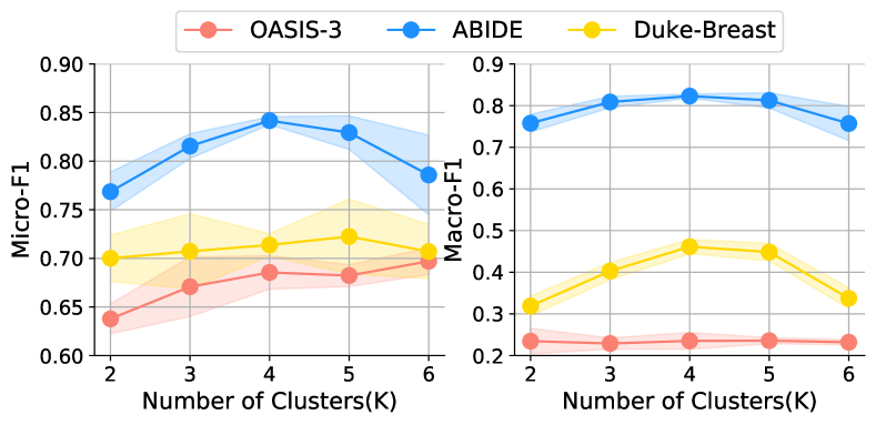
Figure 4: Effect of number of clusters $|R|$.

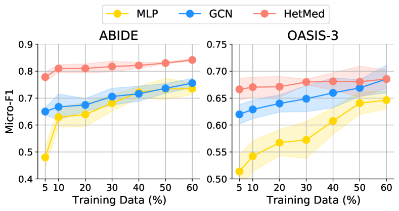
Figure 5: Effect of number of training data.

Non-Image Features Splitting Strategy. Since a multiplex network in HetMed is constructed based on non-overlapping $|R|$ types of non-image features, it is important to have splits such that each type contains its own meaningful information. In this regard, we compare the performance of HetMed with various feature splitting strategies in Table 5: i) splitting features randomly, and ii) splitting features based on domain knowledge. We have the following observations: 1) Our proposed clustering-based splitting strategy outperforms the random splitting strategy. We attribute this to the fact that the randomly split feature types may share similar features with one another, which hinders the construction of a meaningful multiplex network. 2) Splitting non-image features based on domain knowledge outperforms the clustering-based strategy. We argue that feature types that are split based on domain knowledge are clinically more meaningful, which eventually leads to a multiplex network that better captures complex relationship between patients that is clinically more meaningful. It is important to note that with some help of clinicians, the performance can be further improved, which implies that our HetMed can serve as a clinical decision support tool. Note that splitting based on domain knowledge can be considered as an upper bound of clustering-based splitting strategy.

Number of Training Data. Since a large volume of annotated data is rarely available in medical domain, showing robustness under the lack of labeled data is a key challenge in medical image analysis. As shown in Figure 5, HetMed consistently produces accurate predictions even under the lack of labeled data, and the performance gap becomes larger as the number of training data gets smaller, which demonstrates the practicality of HetMed. By modeling complex relationship into a multiplex network, HetMed becomes more robust than single relationship network (i.e., GCN). We can also observe that graph-based methods (i.e., GCN and HetMed) are more robust than non graph-based method (i.e. MLP). This is due to the advantage of using graph neural networks which makes decision by aggregating information from neighborhoods even with lack of label information. Moreover, we further verify the robustness of HetMed under the number of features used in Appendix 7.5.

5.4 Model Practicality

Explainability. The explainability of a machine learning model is one of the most important factors in its application to the medical field. Thanks to the attentive pooling mechanism in HetMed that captures the importance of each relation type, HetMed can provide explanations on which relationship has the most significant effect on the target disease. In Figure 9(a), we find out that model attention weights are concentrated on Type 3 relationship (i.e., cognitive abilities). This indicates that cognitive ability is the most important factor in determining Alzheimer’s disease among the multiple clinical features. Furthermore, in Figure 9(b), we conduct case studies on two patients, i.e., Patient A and Patient B, with Alzheimer Disease (AD) (i.e., CDR 2), who are correctly classified as having AD by HetMed, but incorrectly classified as not having AD by GCN. We calculate the average pairwise cosine similarity of non-image feature between patients A/B, and other patients that belong to different classes. We find out that when computing the similarity based on all the features, patients A and B are expected to belong to CDR 0.5 (i.e., very mild impairment) and CDR 0 (i.e., normal), respectively. However, when the similarities are computed based only on Type 3 feature discovered by HetMed to be important for the target disease, we observe that both patients A and B show the highest similarity with patients that belong to CDR 2 (i.e., moderate dementia). This implies that HetMed can infer the importance of each feature type, which can be used to explain the model prediction. We further verify explainability on various datasets in Appendix 7.5.

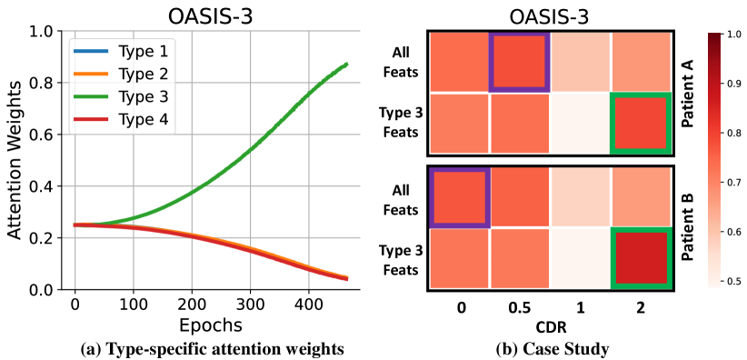
Figure 6: Model explainability analysis.

Generalizability. To further verify the practicality of HetMed, we conduct experiments on the situations where new patients arrive at the hospital (Table 6). We assume that new patients have provided all the required information to the hospital, which means these patients have their own medical image and non-image data. Under this situation, existing non graph-based approaches (e.g., MLP) would classify the patients based on their features alone. On the other hand, benefiting from the inductive capability of graph neural networks (Hamilton, Ying, and Leskovec 2017), we propose to add the new patients into the graph that we have used for training, and classify them based on the trained model. More precisely, we first split the non-image features of the new patients into $|R|$ types of features found during training, and follow Equation 2 to connect them to existing patients. Having constructed the graph, we use the trained multiplex graph neural networks to obtain the embeddings for the new patients, which are then used for classification. For experiments, we split the data into train/validation/test data into 60/10/30%, and use the graph that consists of patients that belong to the train split during the model training. We report the performance on the test data when the performance on the validation data is the best. We observe that graph-based methods (i.e., GCN and HetMed) perform better than a non graph-based method (i.e., MLP), which demonstrates the benefit of leveraging the relationship between patients. Moreover, HetMed outperforms GCN, which again verifies that considering various relationships between patients is crucial. We argue that this experiment demonstrates the practicality of HetMed.

Model	OASIS-3		Duke-Breast		CMMD
	Ma-F1	Mi-F1	Ma-F1	Mi-F1	Ma-F1	Mi-F1
MLP	0.197	0.646	0.359	0.622	0.484	0.642
	(0.017)	(0.029)	(0.011)	(0.023)	(0.028)	(0.053)
GCN	0.203	0.674	0.360	0.653	0.592	0.670
	(0.016)	(0.015)	(0.023)	(0.006)	(0.018)	(0.027)
HetMed	0.217	0.684	0.362	0.742	0.631	0.748
	(0.009)	(0.012)	(0.012)	(0.032)	(0.014)	(0.013)

Table 6: Performance on generalization.

6 Conclusion

In this paper, we propose a general framework called HetMed for fusing multiple modalities of medical data, which provides heterogeneous and complementary information on a single patient. Instead of naively fusing medical data, we propose to fuse multiple modalities into a multiplex network that contains complex relational information between patients. By doing so, the proposed framework HetMed captures important information for clinical decision by considering various aspects of the given data. Through experiments on the variety of multi-modal medical data, we empirically show the effectiveness of HetMed in fusing multiple modalities. A further appeal of HetMed is explainability and generalizability, which demonstrates the practicality of HetMed.

7 Appendix

7.1 Datasets

To evaluate HetMed, we use three brain related datasets, i.e., Alzheimer’s Disase Neuroimaging Intitiative (ADNI) (Petersen et al. 2010), Open Access Series of Imaging Studies (OASIS-3) (LaMontagne et al. 2019) and Autism Brain Imaging Data Exchange (ABIDE) (Di Martino et al. 2014, 2017), and two breast-related datasets, i.e., Dynamic contrast-enhanced magnetic resonance images of breast cancer patients with tumor locations (Duke-Breast) (Saha et al. 2021, 2018; Clark et al. 2013) and Chines Mammography Dataset (CMMD) (Cai et al. 2019; Wang et al. 2016).

• ADNI (Petersen et al. 2010): Alzheimer’s Disease Neuroimaging Initiative (ADNI) is a collection of multiple types of medical images (i.e., MRI, PET, DTI) and non-image clinical data (i.e., genetic information, clinical information and cognitive tests) that are related to Alzheimer’s disease. ADNI is an ongoing project that consists of different studies, i.e., ADNI 1, ADNI 2, ADNI 3, ADNI - GO. In our study, we use ADNI 1 dataset with T3-weighted MRI scan. In this subset, total 417 individuals are comprised of 135 cognitive normal subjects, 203 subjects with late mild cognitive impairment, and 79 subjects with Alzheimer’s disease.

• OASIS-3 (LaMontagne et al. 2019): Open Access Series of Imaging Studies (OASIS-3) provides openly shared neuro-image, clinical and cognitive data for research purpose. OASIS-3 comprises of 1,379 subjects with 2,842 MR sessions, 2,157 PET sessions and 1,472 CT sessions. The participants of OASIS-3 include 755 cognitively normal and 622 individuals at various stages of cognitive decline ranging in age from 42-95yrs. Among the subjects, we select 979 subjects who have both modalities of medical data and have T1-weighted MRI images. Those 979 subjects are divided into 4 groups according to the various CDR level, i.e., 670 subjects with CDR 0, 189 subjects with CDR 0.5, 38 subjects with CDR 1 and 82 subjects with CDR 2.

• ABIDE (Di Martino et al. 2014, 2017): Autism Brain Imaging Data Exchange (ABIDE) dataset has been used to detect autism spectrum disorder based on brain imaging. ABIDE involves 20 different sites, shares resting state functional magnetic resonance imaging (R-fMRI), anatomic, phenotype and clinical information of 1,112 subjects. We select 977 subjects in same pipeline of MRI scans processing. The subjects comprised 473 individuals with autism spectrum disorder and 504 healthy controls individuals.

• Duke-Breast (Saha et al. 2021, 2018): Dynamic contrast-enhanced magnetic resonance images of breast cancer patients with tumor locations (Duke-Breast) has been published by The Cancer Imaging Archive (TCIA) (Clark et al. 2013). It provides medical images and non-image clinical data for prediction of tumor. Among 922 patient IDs, we select 614 IDs that consists of 44 IDs with tumor grade 1.0, 105 IDs with tumor grade 2.0, and 465 IDs with tumor grade 3.0.

• CMMD (Cai et al. 2019; Wang et al. 2016): Chinese Mammography Dataset (CMMD) has also been published by TCIA for early stage diagnosis on breast cancer. It includes 1,775 mammography studies from 1,775 patients in various Chinese institutions between 2012 and 2016. Among the patients, we select 1774 subsets that consists of 481 benign and 1293 malignant patients.

	Learning	Embedding	Number of	Graph	$\alpha$	$\beta$	$\gamma$
	rate ($\eta$)	dim ($d$)	Clusters ($|R|$)	Thres. ($\theta$)
ADNI	0.0005	256	4	(0.9,0.9,0.9,0.9)	0.001	0.1	0.0001
OASIS-3	0.0001	128	4	(0.75,0.75,0.9,0.9)	0.001	0.1	0.0001
ABIDE	0.0005	64	4	(0.9,0.9,0.9,0.9)	0.001	1.0	0.0001
Duke-Breast	0.0005	64	4	(0.75,0.9,0.75,0.75)	0.001	0.01	0.0001
CMMD	0.0001	64	4	(0.9,0.9,0.9,0.75)	0.001	0.01	0.0001

Table 7: Hyperparameter specifications of HetMed.

7.2 Compared Methods

In this section, we explain methods that are compared in the experiments.

• Feature Fusion (Holste et al. 2021) concatenates the medical image data features obtained from a image encoder and features obtained from non-image medical data, and jointly train to produce a final prediction.

• Probability Fusion (Holste et al. 2021) combines the output probabilities of the independently trained models, i.e., image-only and non-image-only models, to produce a final prediction.

• Learned Feature Fusion (Holste et al. 2021) learns features from the image data and non-image data simultaneously, and uses the learned feature vectors to produce a final prediction.

• Spectral (Parisot et al. 2017) leverages a graph structure for fusing multiple modalities. Specifically, each node indicates a patient and each edge indicates the similarity between patients. However, this model uses dataset specific features for each node, i.e., vectorized functional connectivity matrix for ABIDE dataset and volumes of all 139 segmented brain structures for ADNI dataset, which hinders generality of the framework. In our experiments, we use extracted image features as node feature for fair comparisons.

• MLP replaces Multiplex Graph Neural Networks in HetMed with a simple Multi-layer Perceptron (MLP). That is, MLP is trained to predict labels given concatenated vector of image and non-image feature.

• GCN replaces Multiplex Graph Neural Networks in HetMed with a simple Graph Neural Networks (GNN) (Kipf and Welling 2016). It only considers a single relationship between patients instead of multiple relationships as in our proposed multiplex network neural network.

7.3 Evaluation Metrics

We evaluate the model performance in terms of Macro-F1 and Micro-F1 defined as follows:

$${\text{Precision}_{macro}=\frac{\sum_{k=1}^{K}{\text{Precision}_{k}}}{K}}$$ (7)

$${\text{Recall}_{macro}=\frac{\sum_{k=1}^{K}{\text{Recall}_{k}}}{K}}$$ (8)

$${\text{Macro-F1}=2\times\frac{\text{Precision}_{macro}\times\text{Recall}_{macro}}{\text{Precision}_{macro}+\text{Recall}_{macro}}}$$ (9)

$${\text{Precision}_{micro}=\frac{\sum_{k=1}^{K}{\text{TP}_{k}}}{\sum_{k=1}^{K}{\text{TP}_{k}+\text{FP}_{k}}}}$$ (10)

$${\text{Recall}_{micro}=\frac{\sum_{k=1}^{K}{\text{TP}_{k}}}{\sum_{k=1}^{K}{\text{TP}_{k}+\text{FN}_{k}}}}$$ (11)

$${\text{Micro-F1}=2\times\frac{\text{Precision}_{micro}\times\text{Recall}_{micro}}{\text{Precision}_{micro}+\text{Recall}_{micro}}}$$ (12)

where Precision_k $=\mathrm{TP}_{k}/(\mathrm{TP}_{k}+\mathrm{FP}_{k})$, Recall_k $=\mathrm{TP}_{k}/(\mathrm{TP}_{k}+\mathrm{FN}_{k})$, TP_k, TN_k, FP_k, and FN_k denote precision, recall and the number of true positives, true negatives, false positives, and false negatives for class $k$, respectively. Note that in mutlti-class classification where each observation has a single label, Micro-F1 is equivalent to Accuracy.

7.4 Implementation Details

As described in Section 5.1 of the submitted manuscript, we use ResNet-18 (He et al. 2016) as our backbone image encoder $f(\cdot)$. Moreover, we use GCN (Kipf and Welling 2016) encoders for multiplex network training. The base encoder of HetMed is a GCN model followed by an activation function. More formally, the architecture of the encoder $g_{r}(\cdot)$ is defined as:

$$\mathbf{H}^{(r)}=\mathrm{GCN}^{(r)}\mathbf{(X,A)}=\sigma(\mathbf{\hat{D}}^{-1/2}\mathbf{\hat{A}}\mathbf{\hat{D}}^{-1/2}\mathbf{XW}^{(r)}),$$ (13)

where $\mathbf{H}^{(r)}$ is the type $r$ node embedding matrix, $\hat{\mathbf{A}}^{(r)}=\mathbf{A}^{(r)}+\mathbf{I}$ is the type $r$ adjacency matrix with self-loops, $\hat{\mathbf{D}}^{(r)}=\sum_{i}{\hat{\mathbf{{A}}}^{(r)}_{i}}$ is the type $r$ degree matrix, $\sigma(\cdot)$ is a nonlinear activation function such as ReLU, and $\mathbf{W}^{(r)}$ is the trainable weight matrix for type $r$ relationship.

End-to-end Framework for 2D Medical Images. For the experiments regarding the end-to-end framework (Table 2 in Section 5.2), we use ResNet-18 model without any pretrained weights. By directly using medical image representation $\mathbf{Z}$ and non-image feature $\mathbf{C}$ as an input of multiple network, ResNet is also being trained during whole training process.

Pretraining Framework for 2D Medical Images. For the experiments regarding the pretraining framework (Table 3 in Section 5.2), we pretrain ResNet-50 with non-medical image dataset, i.e., SimCLR and MoCo. Specifically, we use pretrained weights that are provided in github repos. With the pretrained ResNet-50, we additionally train the model with medical image through MICLe loss. Then, the weights of ResNet model is fixed during training of multiplex graph neural network.

3D Medical Images. For the experiments regarding 3D medical images (Table 4 in Section 5.2), we follow pretraining scheme of Table 4 in Section 5.2, i.e., we first pretrain the ResNet model with 3D self-supervised medical image representation learning methods, i.e., Jigsaw, Rotation, Exemplar, and freeze the weights of the pretrained model during training multiplex graph neural network.

We tune the model hyperparameters in certain ranges as described in submitted manuscript. The best performing hyperparameters are reported in Table 7.

7.5 Additional Experiments

Importance of Multi-Modality

As mentioned in Section 1 of the submitted manuscript, multiple modalities of medical data provide different and complementary views of the same patient. To corroborate our argument, we conduct case studies by calculating average pairwise cosine similarity of features between a certain patient and all other patients in various classes (Figure 7). Specifically, we calculate the average of feature similarities based on 1) only image data, 2) only non-image data, and 3) both image and non-image data. To calculate the image-only similarity, we use the image representations produced by a pretrained image encoder. To calculate the non-image only similarities, we use the raw non-image features given in each dataset. To calculate the similarities based on both image and non-image data, we concatenate the image representations and non-image features, and use them for calculations.

We observe in Figure 7 (a) that a patient with CDR 0.5 is shown to be similar to patients with CDR 0 when using only medical image data. On the other hand, the patient is shown to be similar to CDR 1 when using only non-image data. This shows that multiple modalities of medical data provide different views both of which may be incorrect. That is, in this case, if the model is based only on the image data, a proactive medical decision would be dangerous since the model turns out to underestimate the situation. On the other hand, if the model is based only on the non-image data, the patient might suffer from various side effects (e.g., dizziness, insomnia, headache, etc.) since the model overestimates the situation which leads to over-treatments. However, by incorporating both modalities (i.e. Img.+Non-Img. in Figure 7 (a)), the model provides patients with accurate clinical decisions, which facilitates a proactive medical decision and a prevention of over-treatments. Figure 7 (b) shows another case study in which considering both modalities at the same time can only provide a correct clinical decision.

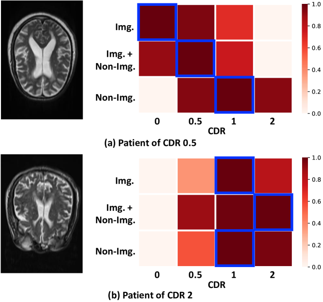
Figure 7: Case Study on OASIS-3 dataset. The element with the highest similarity value in each row is marked with a blue square.

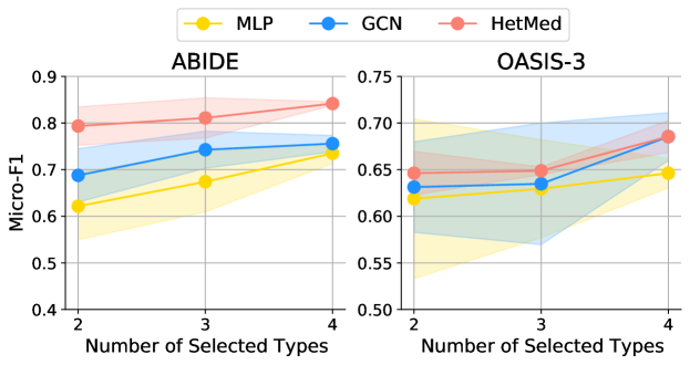
Figure 8: Effect of number of non-image features.

$|R|$	Method	OASIS-3		ABIDE
		Macro	Micro	Macro	Micro
1	Spec.	0.220	0.669	0.649	0.776
		(0.211)	(0.020)	(0.010)	(0.011)
	F.C.	0.202	0.648	0.701	0.717
	w/ weight	(0.018)	(0.034)	(0.048)	(0.029)
	GCN	0.235	0.685	0.751	0.756
		(0.025)	(0.026)	(0.016)	(0.018)
4	Multiplex	0.235	0.686	0.833	0.842
		(0.020)	(0.017)	(0.005)	(0.004)

Table 8: Performace on various edge construction strategies.

Model	ADNI		OASIS-3		ABIDE		Duke-Breast		CMMD
	Ma-F1	Mi-F1	Ma-F1	Mi-F1	Ma-F1	Mi-F1	Ma-F1	Mi-F1	Ma-F1	Mi-F1
MLP	0.561	0.781	0.219	0.646	0.703	0.735	0.430	0.652	0.523	0.751
	(0.022)	(0.031)	(0.017)	(0.016)	(0.023)	(0.022)	(0.019)	(0.019)	(0.027)	(0.014)
GCN	0.611	0.816	0.235	0.685	0.751	0.756	0.440	0.698	0.625	0.745
	(0.019)	(0.014)	(0.025)	(0.026)	(0.016)	(0.018)	(0.017)	(0.019)	(0.014)	(0.022)
HAN	0.801	0.823	0.221	0.677	0.829	0.834	0.434	0.745	0.719	0.779
	(0.015)	(0.023)	(0.014)	(0.017)	(0.022)	(0.031)	(0.028)	(0.034)	(0.019)	(0.027)
GATNE	0.812	0.820	0.226	0.669	0.799	0.802	0.423	0.785	0.705	0.767
	(0.018)	(0.014)	(0.008)	(0.020)	(0.023)	(0.018)	(0.010)	(0.032)	(0.019)	(0.015)
DMGI	0.851	0.857	0.235	0.686	0.833	0.842	0.447	0.765	0.720	0.781
	(0.009)	(0.012)	(0.020)	(0.017)	(0.005)	(0.004)	(0.011)	(0.021)	(0.025)	(0.022)

Table 9: Various Multiplex Network Embedding.

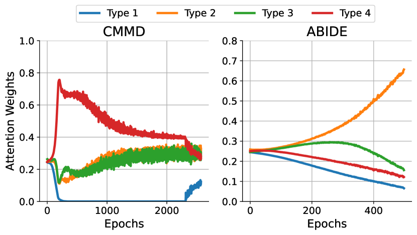
Figure 9: Additional analyses on the learned attention weights.

Number of Non-Image Features

In this section, we further verify the benefit of using multiplex network, which is shown in Section 5.3 in the submitted manuscript, i.e. robustness of multiplex network. In this experiment, we use certain types of features during the whole experiment. Specifically, we split non-image medical data into $|R|$ types as done before, but use only a subset among the $\mathbf{T}=\{T_{1},T_{2},\cdots,T_{|R|}\}$ feature types. By doing so, we can verify the robustness of the multiplex network-based approach under certain types of information loss. Note that we averaged over the performance of all possible combinations. For example, if only two types among four are used, we get $\binom{4}{2}=6$ combinations in total, and we average over the results for all six combinations. As shown in Figure 8, HetMed shows robustness even when only few feature types are used. We argue that modeling complex relationships through a multiplex network not only benefits the model in terms of performance but also robustness.

Edge Construction Strategies

In Table 8, we adopt various graph construction strategies proposed in previous works (Parisot et al. 2017; Cao et al. 2021). Parisot et al. (2017) (Spec.) constructs a graph by comparing absolute values of certain features leading to an almost fully connected graph, while Cao et al. (2021) (F.C. w/ weight) constructs a fully connected graph with edge weights whose weights are given by the similarity between the connected patients. Among various graph construction methods, HetMed based on a multiplex network shows the best performance, indicating the benefit of modeling complex relationship among patients. On the other hand, we find out that constructing a single graph with cosine similarity (i.e., GCN) outperforms other single graph construction strategies. We attribute this to the shortcomings of previous works, which connects almost every patient without regarding the informativeness of the relationships. That is, fully connected graph may inject noise to the model when aggregating the messages from connected patients.

Attention Analysis

In addition to the analysis reported in Figure 6 (a) of the submitted manuscript, we additionally provide analyses on the attention weights learned by HetMed on other datasets used in the experiments, i.e., CMMD and ABIDE datasets, in Figure 9. In ABIDE dataset, we observe that the attention weights are concentrated on the Type 2 relationship, which is about stereotyped behaviors, restricted interest and social responsiveness score. Compared with Type 3 relationship, which is about social effect, responsiveness and resticted behavior, it is obvious that the features in the Type 2 relationship are more crucial for identifying autism, and this is automatically detected by HetMed. Furthermore, despite their fairly similar information, we find out that graph $\mathcal{G}^{(2)}$, i.e., a graph constructed by the Type 2 features, captures more informative relationship than $\mathcal{G}^{(3)}$, i.e., a graph constructed by the Type 3 features, since the social responsiveness score (i.e., SRS_RAW_TOTAL feature) in the Type 2 features captures more fine-grained relationship between patients than other ADOS information about social effect and responsiveness in Type 3. On the other hand, in CMMD dataset, all types show nearly the same attention weights when identifying breast tumor. This is because, all types of features are closely related to the diagnosis of tumor due to the lack of information.

Various Multiplex Network Embedding

To further verify that HetMed is a model-agnostic framework, we adopt various recent multiplex network embedding methods (i.e., HAN (Wang et al. 2019) and GATNE (Cen et al. 2019)) into HetMed, and report results in Table 9. We have the following observations: 1) We find out that HetMed with various multiplex network embedding methods outperform existing other simple fusion methods (i.e., MLP and GCN), verifying the generality of HetMed. 2) DMGI outperforms all other multiplex network embedding methods, indicating modeling complex relationship between patients through consensus regularization and attentive mechanism are effective.

Feature Clustering Analysis

Table 10 shows the features categorized based on HetMed and domain knowledge. In general, we observe that our proposed column-wise K-means clustering tends to categorize similar features into the same group. For example in ADNI dataset, features that are related to simple memory tasks are grouped into Type 2 features, while features that are related to sophisticated memory tasks are grouped into Type 3 features. Moreover, in ABIDE dataset, Type 1 features include patient specific information while Type 2 includes detailed information regarding social responsiveness and behavior scores. We argue that by categorizing similarly characterized features into the same group, each of these groups captures distinct information, which helps to capture the complex relational information between patients. Note that details of the features that are split based on domain knowledge reported in the experiments regarding Table 5 of the submitted manuscript can be also found in Table 10.

7.6 Pseudocode of HetMed

Algorithm 1 shows the pseudocode of HetMed.

Input : A input image matrix $\mathbf{B}$, A input non-image matrix $\mathbf{C}$, A label matrix $\mathbf{Y}$, Number of clusters $|R|$, Thresholds $\mathbf{\theta}$, Maximum epoch of image training $MaxEpoch_{i}$, Maximum epoch of fusion training $MaxEpoch_{f}$, Image encoder $f$, Graph encoder $g$.

1 if 2D Image then

2       Pretrain with non-medical image

3 end if

4while not $MaxEpoch_{i}$ do

5       $\mathcal{L}^{\mathrm{Image}}\leftarrow\textsf{run}_{image}(\mathbf{B})$

6       Update f by backpropagating $\mathcal{L}^{Image}$

7 end while

// Learn medical img. representations

8 Cluster $\mathbf{C}$ into $\mathbf{C}^{(r)}\leftarrow\left\{\mathbf{C}^{(1)},\mathbf{C}^{(2)}\ldots,\mathbf{C}^{(|R|)}\right\}$

9 for $r=1,2,\ldots,|R|$ do

10       $\mathbf{A}^{(r)}(i,j)=\begin{cases}1&\mbox{if }\rho^{(r)}(i,j)>\theta^{(r)},\\ 0&\mbox{otherwise, }\end{cases}$

11 end for

12$\mathbf{Z}\leftarrow f(\mathbf{B})$

13 $\mathbf{X}\leftarrow Concatenate(\mathbf{Z},\mathbf{C})$

// Multiplex network construction

14 while not $MaxEpoch_{f}$ do

15       $\mathcal{L}^{\mathrm{Fusion}}\leftarrow\textsf{run}_{fusion}(\mathbf{X},\mathbf{A}^{(1)},\mathbf{A}^{(2)},\ldots,\mathbf{A}^{(|R|)})$

16       Update $g$ by backpropagating $\mathcal{L}^{\mathrm{Fusion}}$

17      

18 end while

// Train multiplex GNNs

19

20Function $\textsf{run}_{image}$($\mathbf{B}$):

21       $\mathbf{Z}\leftarrow f(\mathbf{B})$

22       if 2D Image then

23             $\mathcal{L}^{\mathrm{Image}}\leftarrow\sum_{i=1}^{|V|}\mathcal{L}_{i}^{\mathrm{MICLe}}$

24       else

25            $\mathcal{L}^{\mathrm{Image}}\leftarrow\mathcal{L}^{\mathrm{3D-Image}}$

26       end if

27      return $\mathcal{L}^{\mathrm{Image}}$

28 end

29

30

31Function $\textsf{run}_{fusion}$($\mathbf{X},\mathbf{A}^{(1)},\mathbf{A}^{(2)},\ldots,\mathbf{A}^{(|R|)}$):

32      

33      for $r=1,2,\ldots,|R|$ do

34             $\mathbf{H}^{(r)},\tilde{\mathbf{H}}^{(r)}\leftarrow g_{r}(\mathbf{X},\mathbf{A}^{(r)}),g_{r}(\tilde{\mathbf{X}},\mathbf{A}^{(r)})$

35       end for

36      

37      $\mathcal{L}^{\mathrm{Fusion}}\leftarrow\sum_{r\in\mathcal{R}}{\mathcal{L}^{(r)}}+\alpha\ell_{cs}+\beta\ell_{sup}+\gamma\|\boldsymbol{\Theta}\|^{2}$

38      return $\mathcal{L}^{\mathrm{Fusion}}$

39 end

Algorithm 1 Pseudocode for HetMed.

Dataset	Type	Ours	Domain
			Knowledge
ADNI	1	ADASQ4, RAVLT_forgetting, TRABSCOR	Hippocampus, Entorhinal
	2	MMSE, RAVLT_immediate, RAVLT_learning, LDELTOTAL,	RAVLT_immediate, RAVLT_learning, RAVLT_forgetting,
		DIGITSCOR, mPACCdigit, mPACCtrailsB, Hippocampus, Entorhinal	RAVLT_perc_forgetting, LDELTOTAL, DIGITSCOR
	3	CDRSB, ADAS11, ADAS13, FAQ	CDRSB, ADAS13, ADAS11, TRABSCOR, FAQ, ADASQ4
	4	RAVLT_perc_forgetting	MMSE, mPACCdigit, mPACCtrailsB
OASIS-3	1	HIS and CVD, NPI-Q, age, apoe, homehobb	Psych Assessments, Informant Demos,
			ADRC Clinical Data, Clinician Diagnosis
	2	Partcpt Family Hist., Sub Health Hist.,	Phys. Neuro Findings, UPDRS, DECCLIN,
		UPDRS, ADRC Clinical Data, DECCLIN, DECIN	DECIN, FAQs, Clin. Judgements
	3	Psych Assessments, FAQs, Sub Demos, Clin. Judgements	Sub Health Hist., GDS, Partcpt Family Hist.
	4	Clinician Diagnosis, GDS, Phys. Neuro Findings, Informant Demos	age, NPI-Q, HIS and CVD, Sub Demos
ABIDE	1	HANDEDNESS_CATEGORY, AGE_AT_SCAN, SEX, FIQ, EYE_STATUS_AT_SCAN	AGE_AT_SCAN, SEX, SRS_RAW_TOTAL
	2	HANDEDNESS_SCORES, ADOS_STEREO_BEHAV, SRS_RAW_TOTAL	EYE_STATUS_AT_SCAN, HANDEDNESS_CATEGORY,
			ADOS_GOTHAM_SOCAFFECT
	3	ADOS_GOTHAM_SOCAFFECT, ADOS_GOTHAM_RRB, ADOS_GOTHAM_TOTAL, ADOS_GOTHAM_SEVERITY	ADOS_GOTHAM_SEVERITY, HANDEDNESS_SCORES,
			ADOS_STEREO_BEHAV, ADOS_GOTHAM_RRB,
			ADOS_GOTHAM_TOTAL,
	4	VIQ, PIQ	VIQ, PIQ, FIQ
Duke-Breast	1	Menopause (at diagnosis), ER, PR, Surgery, Adjuvant Radiation Therapy,	Staging(Nodes)#(Nx replaced by -1)[N], HER2, ER, PR,
		Adjuvant Endocrine Therapy Medications, Pec/Chest Involvement	Staging(Metastasis)#(Mx -replaced by -1)[M]
	2	HER2, Multicentric/Multifocal, Lymphadenopathy or Suspicious Nodes,	Menopause (at diagnosis), Metastatic at Presentation (Outside of Lymph Nodes)
		Definitive Surgery Type, Neoadjuvant Chemotherapy, Adjuvant Chemotherapy,	Adjuvant Chemotherapy, Adjuvant Endocrine Therapy Medications,
		Neoadjuvant Anti-Her2 Neu Therapy, Adjuvant Anti-Her2 Neu Therapy	Known Ovarian Status, Recurrence event(s)
	3	Metastatic at Presentation (Outside of Lymph Nodes), Contralateral Breast Involvement	Surgery, Definitive Surgery Type, Neoadjuvant Radiation Therapy
		Staging(Metastasis)#(Mx -replaced by -1)[M], Skin/Nipple Involvement,	Neoadjuvant Chemotherapy, Adjuvant Radiation Therapy
		Neoadjuvant Radiation Therapy, Recurrence event(s), Known Ovarian Status,	Neoadjuvant Anti-Her2 Neu Therapy, Adjuvant Anti-Her2 Neu Therapy
		Therapeutic or Prophylactic Oophorectomy as part of Endocrine Therapy,	Therapeutic or Prophylactic Oophorectomy as part of Endocrine Therapy
		Neoadjuvant Endocrine Therapy Medications	Neoadjuvant Endocrine Therapy Medications
	4	Staging(Nodes)#(Nx replaced by -1)[N]	Multicentric/Multifocal, Lymphadenopathy or Suspicious Nodes
			Pec/Chest Involvement, Contralateral Breast Involvement, Skin/Nipple Invovlement
CMMD	1	LeftRight	LeftRight
	2	abnormality	abnormality
	3	subtype	subtype
	4	age	age

Table 10: Feature Split based on K-means clustering (Ours) and Domain Knowledge.

References

- Aggarwal et al. (2021) Aggarwal, R.; Sounderajah, V.; Martin, G.; Ting, D. S.; Karthikesalingam, A.; King, D.; Ashrafian, H.; and Darzi, A. 2021. Diagnostic accuracy of deep learning in medical imaging: A systematic review and meta-analysis. NPJ digital medicine, 4(1): 1–23.
- Akselrod-Ballin et al. (2019) Akselrod-Ballin, A.; Chorev, M.; Shoshan, Y.; Spiro, A.; Hazan, A.; Melamed, R.; Barkan, E.; Herzel, E.; Naor, S.; Karavani, E.; et al. 2019. Predicting breast cancer by applying deep learning to linked health records and mammograms. Radiology, 292(2): 331–342.
- Azizi et al. (2021) Azizi, S.; Mustafa, B.; Ryan, F.; Beaver, Z.; Freyberg, J.; Deaton, J.; Loh, A.; Karthikesalingam, A.; Kornblith, S.; Chen, T.; et al. 2021. Big self-supervised models advance medical image classification. In Proceedings of the IEEE/CVF International Conference on Computer Vision, 3478–3488.
- Cai et al. (2019) Cai, H.; Huang, Q.; Rong, W.; Song, Y.; Li, J.; Wang, J.; Chen, J.; and Li, L. 2019. Breast microcalcification diagnosis using deep convolutional neural network from digital mammograms. Computational and mathematical methods in medicine, 2019.
- Cao et al. (2021) Cao, M.; Yang, M.; Qin, C.; Zhu, X.; Chen, Y.; Wang, J.; and Liu, T. 2021. Using DeepGCN to identify the autism spectrum disorder from multi-site resting-state data. Biomedical Signal Processing and Control, 70: 103015.
- Cen et al. (2019) Cen, Y.; Zou, X.; Zhang, J.; Yang, H.; Zhou, J.; and Tang, J. 2019. Representation learning for attributed multiplex heterogeneous network. In Proceedings of the 25th ACM SIGKDD International Conference on Knowledge Discovery & Data Mining, 1358–1368.
- Cheerla and Gevaert (2019) Cheerla, A.; and Gevaert, O. 2019. Deep learning with multimodal representation for pancancer prognosis prediction. Bioinformatics, 35(14): i446–i454.
- Chen et al. (2020) Chen, T.; Kornblith, S.; Norouzi, M.; and Hinton, G. 2020. A simple framework for contrastive learning of visual representations. In International conference on machine learning, 1597–1607. PMLR.
- Clark et al. (2013) Clark, K.; Vendt, B.; Smith, K.; Freymann, J.; Kirby, J.; Koppel, P.; Moore, S.; Phillips, S.; Maffitt, D.; Pringle, M.; et al. 2013. The Cancer Imaging Archive (TCIA): maintaining and operating a public information repository. Journal of digital imaging, 26(6): 1045–1057.
- Coates, Ng, and Lee (2011) Coates, A.; Ng, A.; and Lee, H. 2011. An analysis of single-layer networks in unsupervised feature learning. In Proceedings of the fourteenth international conference on artificial intelligence and statistics, 215–223. JMLR Workshop and Conference Proceedings.
- Cui et al. (2022) Cui, C.; Yang, H.; Wang, Y.; Zhao, S.; Asad, Z.; Coburn, L. A.; Wilson, K. T.; Landman, B. A.; and Huo, Y. 2022. Deep Multi-modal Fusion of Image and Non-image Data in Disease Diagnosis and Prognosis: A Review. arXiv preprint arXiv:2203.15588.
- De Domenico et al. (2013) De Domenico, M.; Solé-Ribalta, A.; Cozzo, E.; Kivelä, M.; Moreno, Y.; Porter, M. A.; Gómez, S.; and Arenas, A. 2013. Mathematical formulation of multilayer networks. Physical Review X, 3(4): 041022.
- Deng et al. (2009) Deng, J.; Dong, W.; Socher, R.; Li, L.-J.; Li, K.; and Fei-Fei, L. 2009. Imagenet: A large-scale hierarchical image database. In 2009 IEEE conference on computer vision and pattern recognition, 248–255. Ieee.
- Deng et al. (2020) Deng, S.; Zhang, X.; Yan, W.; Chang, E. I.; Fan, Y.; Lai, M.; Xu, Y.; et al. 2020. Deep learning in digital pathology image analysis: a survey. Frontiers of medicine, 14(4): 470–487.
- Di Martino et al. (2017) Di Martino, A.; O’connor, D.; Chen, B.; Alaerts, K.; Anderson, J. S.; Assaf, M.; Balsters, J. H.; Baxter, L.; Beggiato, A.; Bernaerts, S.; et al. 2017. Enhancing studies of the connectome in autism using the autism brain imaging data exchange II. Scientific data, 4(1): 1–15.
- Di Martino et al. (2014) Di Martino, A.; Yan, C.-G.; Li, Q.; Denio, E.; Castellanos, F. X.; Alaerts, K.; Anderson, J. S.; Assaf, M.; Bookheimer, S. Y.; Dapretto, M.; et al. 2014. The autism brain imaging data exchange: towards a large-scale evaluation of the intrinsic brain architecture in autism. Molecular psychiatry, 19(6): 659–667.
- Doersch, Gupta, and Efros (2015) Doersch, C.; Gupta, A.; and Efros, A. A. 2015. Unsupervised visual representation learning by context prediction. In Proceedings of the IEEE international conference on computer vision, 1422–1430.
- Emrani et al. (2020) Emrani, S.; Arain, H. A.; DeMarshall, C.; and Nuriel, T. 2020. APOE4 is associated with cognitive and pathological heterogeneity in patients with Alzheimer’s disease: a systematic review. Alzheimer’s Research & Therapy, 12(1): 1–19.
- Gidaris, Singh, and Komodakis (2018) Gidaris, S.; Singh, P.; and Komodakis, N. 2018. Unsupervised representation learning by predicting image rotations. arXiv preprint arXiv:1803.07728.
- Guo et al. (2019) Guo, Z.; Li, X.; Huang, H.; Guo, N.; and Li, Q. 2019. Deep learning-based image segmentation on multimodal medical imaging. IEEE Transactions on Radiation and Plasma Medical Sciences, 3(2): 162–169.
- Hamilton, Ying, and Leskovec (2017) Hamilton, W.; Ying, Z.; and Leskovec, J. 2017. Inductive representation learning on large graphs. Advances in neural information processing systems, 30.
- He et al. (2020) He, K.; Fan, H.; Wu, Y.; Xie, S.; and Girshick, R. 2020. Momentum contrast for unsupervised visual representation learning. In Proceedings of the IEEE/CVF conference on computer vision and pattern recognition, 9729–9738.
- He et al. (2016) He, K.; Zhang, X.; Ren, S.; and Sun, J. 2016. Deep residual learning for image recognition. In Proceedings of the IEEE conference on computer vision and pattern recognition, 770–778.
- Holste et al. (2021) Holste, G.; Partridge, S. C.; Rahbar, H.; Biswas, D.; Lee, C. I.; and Alessio, A. M. 2021. End-to-end learning of fused image and non-image features for improved breast cancer classification from mri. In Proceedings of the IEEE/CVF International Conference on Computer Vision, 3294–3303.
- Howell et al. (2017) Howell, J. C.; Watts, K. D.; Parker, M. W.; Wu, J.; Kollhoff, A.; Wingo, T. S.; Dorbin, C. D.; Qiu, D.; and Hu, W. T. 2017. Race modifies the relationship between cognition and Alzheimer’s disease cerebrospinal fluid biomarkers. Alzheimer’s research & therapy, 9(1): 1–10.
- Huang (1997) Huang, Z. 1997. Clustering large data sets with mixed numeric and categorical values. In Proceedings of the 1st pacific-asia conference on knowledge discovery and data mining,(PAKDD), 21–34. Citeseer.
- Jing, Park, and Tong (2021) Jing, B.; Park, C.; and Tong, H. 2021. Hdmi: High-order deep multiplex infomax. In Proceedings of the Web Conference 2021, 2414–2424.
- Jing et al. (2021) Jing, B.; Xiang, Y.; Chen, X.; Chen, Y.; and Tong, H. 2021. Graph-MVP: Multi-View Prototypical Contrastive Learning for Multiplex Graphs. arXiv preprint arXiv:2109.03560.
- Kazi et al. (2019) Kazi, A.; Shekarforoush, S.; Arvind Krishna, S.; Burwinkel, H.; Vivar, G.; Kortüm, K.; Ahmadi, S.-A.; Albarqouni, S.; and Navab, N. 2019. InceptionGCN: receptive field aware graph convolutional network for disease prediction. In International Conference on Information Processing in Medical Imaging, 73–85. Springer.
- Kipf and Welling (2016) Kipf, T. N.; and Welling, M. 2016. Semi-supervised classification with graph convolutional networks. arXiv preprint arXiv:1609.02907.
- LaMontagne et al. (2019) LaMontagne, P. J.; Benzinger, T. L.; Morris, J. C.; Keefe, S.; Hornbeck, R.; Xiong, C.; Grant, E.; Hassenstab, J.; Moulder, K.; Vlassenko, A. G.; et al. 2019. OASIS-3: longitudinal neuroimaging, clinical, and cognitive dataset for normal aging and Alzheimer disease. MedRxiv.
- Lee et al. (2022a) Lee, J.; Oh, Y.; In, Y.; Lee, N.; Hyun, D.; and Park, C. 2022a. GraFN: Semi-Supervised Node Classification on Graph with Few Labels via Non-Parametric Distribution Assignment. arXiv preprint arXiv:2204.01303.
- Lee et al. (2022b) Lee, N.; Hyun, D.; Lee, J.; and Park, C. 2022b. Relational self-supervised learning on graphs. In Proceedings of the 31st ACM International Conference on Information & Knowledge Management, 1054–1063.
- Lee, Lee, and Park (2022) Lee, N.; Lee, J.; and Park, C. 2022. Augmentation-free self-supervised learning on graphs. In Proceedings of the AAAI Conference on Artificial Intelligence, volume 36, 7372–7380.
- Li et al. (2018) Li, J.; Chen, C.; Tong, H.; and Liu, H. 2018. Multi-layered network embedding. In Proceedings of the 2018 SIAM International Conference on Data Mining, 684–692. SIAM.
- Liu et al. (2021) Liu, Z.; Zhong, S.; Liu, Q.; Xie, C.; Dai, Y.; Peng, C.; Chen, X.; and Zou, R. 2021. Thyroid nodule recognition using a joint convolutional neural network with information fusion of ultrasound images and radiofrequency data. European Radiology, 31(7): 5001–5011.
- Lowekamp et al. (2013) Lowekamp, B. C.; Chen, D. T.; Ibáñez, L.; and Blezek, D. 2013. The design of SimpleITK. Frontiers in neuroinformatics, 7: 45.
- Ma et al. (2018) Ma, Y.; Ren, Z.; Jiang, Z.; Tang, J.; and Yin, D. 2018. Multi-dimensional network embedding with hierarchical structure. In Proceedings of the eleventh ACM international conference on web search and data mining, 387–395.
- Morris (1991) Morris, J. C. 1991. The clinical dementia rating (cdr): Current version and. Young, 41: 1588–1592.
- Noroozi and Favaro (2016) Noroozi, M.; and Favaro, P. 2016. Unsupervised learning of visual representations by solving jigsaw puzzles. In European conference on computer vision, 69–84. Springer.
- Parisot et al. (2017) Parisot, S.; Ktena, S. I.; Ferrante, E.; Lee, M.; Moreno, R. G.; Glocker, B.; and Rueckert, D. 2017. Spectral graph convolutions for population-based disease prediction. In International conference on medical image computing and computer-assisted intervention, 177–185. Springer.
- Park et al. (2020) Park, C.; Kim, D.; Han, J.; and Yu, H. 2020. Unsupervised attributed multiplex network embedding. In Proceedings of the AAAI Conference on Artificial Intelligence, volume 34, 5371–5378.
- Petersen et al. (2010) Petersen, R. C.; Aisen, P.; Beckett, L. A.; Donohue, M.; Gamst, A.; Harvey, D. J.; Jack, C.; Jagust, W.; Shaw, L.; Toga, A.; et al. 2010. Alzheimer’s disease neuroimaging initiative (ADNI): clinical characterization. Neurology, 74(3): 201–209.
- Qu et al. (2017) Qu, M.; Tang, J.; Shang, J.; Ren, X.; Zhang, M.; and Han, J. 2017. An attention-based collaboration framework for multi-view network representation learning. In Proceedings of the 2017 ACM on Conference on Information and Knowledge Management, 1767–1776.
- Ranasinghe et al. (2015) Ranasinghe, P.; Cooray, D. N.; Jayawardena, R.; and Katulanda, P. 2015. The influence of family history of hypertension on disease prevalence and associated metabolic risk factors among Sri Lankan adults. BMC public health, 15(1): 1–9.
- Saha et al. (2021) Saha, A.; Harowicz, M.; Grimm, L.; et al. 2021. Dynamic contrast-enhanced magnetic resonance images of breast cancer patients with tumor locations. The Cancer Imaging Archive.
- Saha et al. (2018) Saha, A.; Harowicz, M. R.; Grimm, L. J.; Kim, C. E.; Ghate, S. V.; Walsh, R.; and Mazurowski, M. A. 2018. A machine learning approach to radiogenomics of breast cancer: a study of 922 subjects and 529 DCE-MRI features. British journal of cancer, 119(4): 508–516.
- Sanyal, Kar, and Sarkar (2021) Sanyal, R.; Kar, D.; and Sarkar, R. 2021. Carcinoma type classification from high-resolution breast microscopy images using a hybrid ensemble of deep convolutional features and gradient boosting trees classifiers. IEEE/ACM Transactions on Computational Biology and Bioinformatics.
- Schlichtkrull et al. (2018) Schlichtkrull, M.; Kipf, T. N.; Bloem, P.; Berg, R. v. d.; Titov, I.; and Welling, M. 2018. Modeling relational data with graph convolutional networks. In European semantic web conference, 593–607. Springer.
- Shi et al. (2017) Shi, C.; Li, Y.; Zhang, J.; Sun, Y.; and Yu, P. S. 2017. A survey of heterogeneous information network analysis. IEEE Transactions on Knowledge and Data Engineering, 29(1): 17–37.
- Singh et al. (2020) Singh, S. P.; Wang, L.; Gupta, S.; Goli, H.; Padmanabhan, P.; and Gulyás, B. 2020. 3D deep learning on medical images: a review. Sensors, 20(18): 5097.
- Suk et al. (2014) Suk, H.-I.; Lee, S.-W.; Shen, D.; Initiative, A. D. N.; et al. 2014. Hierarchical feature representation and multimodal fusion with deep learning for AD/MCI diagnosis. NeuroImage, 101: 569–582.
- Sun, Yu, and Batmanghelich (2021) Sun, L.; Yu, K.; and Batmanghelich, K. 2021. Context matters: Graph-based self-supervised representation learning for medical images. In Proceedings of the AAAI Conference on Artificial Intelligence, volume 35, 4874–4882.
- Taleb et al. (2020) Taleb, A.; Loetzsch, W.; Danz, N.; Severin, J.; Gaertner, T.; Bergner, B.; and Lippert, C. 2020. 3d self-supervised methods for medical imaging. Advances in Neural Information Processing Systems, 33: 18158–18172.
- Tan et al. (2020) Tan, W.; Tiwari, P.; Pandey, H. M.; Moreira, C.; and Jaiswal, A. K. 2020. Multimodal medical image fusion algorithm in the era of big data. Neural Computing and Applications, 1–21.
- Teramoto et al. (2016) Teramoto, A.; Fujita, H.; Yamamuro, O.; and Tamaki, T. 2016. Automated detection of pulmonary nodules in PET/CT images: Ensemble false-positive reduction using a convolutional neural network technique. Medical physics, 43(6Part1): 2821–2827.
- Veličković et al. (2017) Veličković, P.; Cucurull, G.; Casanova, A.; Romero, A.; Lio, P.; and Bengio, Y. 2017. Graph attention networks. arXiv preprint arXiv:1710.10903.
- Wang et al. (2016) Wang, J.; Yang, X.; Cai, H.; Tan, W.; Jin, C.; and Li, L. 2016. Discrimination of breast cancer with microcalcifications on mammography by deep learning. Scientific reports, 6(1): 1–9.
- Wang et al. (2019) Wang, X.; Ji, H.; Shi, C.; Wang, B.; Ye, Y.; Cui, P.; and Yu, P. S. 2019. Heterogeneous graph attention network. In The world wide web conference, 2022–2032.
- Wang, Wang, and Guo (2018) Wang, Z.; Wang, S.; and Guo, L. 2018. Novel multi-focus image fusion based on PCNN and random walks. Neural Computing and Applications, 29(11): 1101–1114.
- Xu et al. (2016) Xu, T.; Zhang, H.; Huang, X.; Zhang, S.; and Metaxas, D. N. 2016. Multimodal deep learning for cervical dysplasia diagnosis. In International conference on medical image computing and computer-assisted intervention, 115–123. Springer.
- Yaniv et al. (2018) Yaniv, Z.; Lowekamp, B. C.; Johnson, H. J.; and Beare, R. 2018. SimpleITK image-analysis notebooks: a collaborative environment for education and reproducible research. Journal of digital imaging, 31(3): 290–303.
- Zhu et al. (2020) Zhu, Y.; Xu, Y.; Yu, F.; Liu, Q.; Wu, S.; and Wang, L. 2020. Deep graph contrastive representation learning. arXiv preprint arXiv:2006.04131.