Spurious Symmetry Enhancement and Interaction-Induced Topology in Magnons

Abstract

Linear spin wave theory (LSWT) is the standard technique to compute the spectra of magnetic excitations in quantum materials. In this paper, we show that LSWT, even under ordinary circumstances, may fail to implement the symmetries of the underlying ordered magnetic Hamiltonian leading to spurious degeneracies. In common with pseudo-Goldstone modes in cases of quantum order-by-disorder these degeneracies tend to be lifted by magnon-magnon interactions. We show how, instead, the correct symmetries may be restored at the level of LSWT. In the process we give examples, supported by nonperturbative matrix product based time evolution calculations, where symmetries dictate that there should be a topological magnon gap but where LSWT fails to open up this gap. We also comment on possible spin split magnons in MnF₂ and similar rutiles by analogy to recently proposed altermagnets.

From Néel order in the mid 20th century to skyrmion phases in the 21st, magnetically ordered materials have been a constant source of insights into the collective behavior of matter. The coherent spin wave excitations, or magnons, about these magnetic textures provide invaluable information about magnetic structures and couplings. They are also interesting in their own right: as a window into many-body interactions and quasiparticle breakdown [1], as a platform for investigating band topology [2, 3, 4], and as an essential ingredient in the functioning of many spintronics devices [5].

One of the most useful theoretical tools at our disposal to understand magnons is an expansion in powers of inverse spin $S$ based on the Holstein-Primakoff bosonization of quantum spins [6]. The single particle spectrum arising from spin wave theory to quadratic order (called linear, or non-interacting, spin wave theory) is often used with great success to constrain magnetic couplings from experimental data. This theory is known to fail qualitatively in cases where coupling between single and multi-particle states becomes important for example in highly frustrated magnets and non-collinear spin textures such as the famous triangular lattice antiferromagnet [7, 8, 1], and close to quantum phase transitions [9].

Another, more subtle way, in which linear spin wave theory (LSWT) can fail qualitatively is called order-by-disorder [10, 11, 12, 13] where spurious ground states and symmetry enhancement exist at the semi-classical level that are lifted by fluctuations. In some instances of quantum order-by-disorder, a spurious continuous symmetry forces the presence of a pseudo-Goldstone mode in LSWT where none should be present [14]. In this paper, we focus on a related instance of this physics where, instead of failing to capture degeneracy breaking in the ground state, the LSWT instead does not fully capture symmetries that affect degeneracies higher up in the excitation spectrum [15]. With growing interest in magnon band topology [16, 17, 18, 19, 20, 21, 22, 23, 24, 25, 26, 27, 28, 29, 30, 31, 32, 33, 34, 35, 36], there is additional impetus to understand how to implement symmetries correctly in LSWT as these provide important constraints on the possible topological band structures that can arise [15, 37, 38].

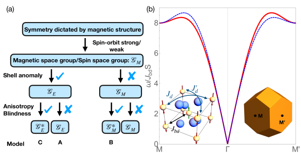
Figure 1: (a) Flow chart indicating the actual and spurious symmetries that may arise in LSWT. The parent symmetry group $\mathcal{G}_{M}$ constrained by the lattice symmetries, magnetic structure and the nature of the exchange may be enhanced via a shell anomaly and/or anisotropy blindness to new symmetry groups denoted $\mathcal{G}^{(*)}_{E}$ or $\mathcal{G}^{*}_{M}$. (b) Spin wave spectrum for a model A exhibiting a shell anomaly in the form of a double degeneracy in the absence of further neighbor terms. The spectrum shown (for the lattice model in the inset) has $J_{d}\neq J^{\prime}_{d}$.

Overview. In many-body physics, there is a large body of work on cases where at long wavelengths and low energies there are enhanced symmetries (e.g. [39, 40]). In contrast, the goals of this paper are to spell out ways in which spin wave theory can lead to spurious degeneracies in excitations across the Brillouin zone and to supply a simple, general way to resolve them.

The cases we consider fall into two classes [see Fig. 1(a)]. The first class is where the lattice symmetries are not manifest for exchange couplings between moments out to $n$th nearest neighbors but where the symmetries do manifest for longer-range couplings. This, we call the shell anomaly. Such a situation may be completely physical and, far from being confined to spin wave theory, it may arise in general tight-binding models. The second class is more subtle: where LSWT does not capture certain kinds of exchange anisotropy or anisotropy blindness. Then, LSWT fails to produce the correct magnon spectrum at a qualitative level and spurious symmetry-protected topological magnon degeneracies occur. We show that degeneracy breaking occurs by carrying out DMRG plus matrix product operator time evolution (DMRG+tMPO) [41, 42, 43] to resolve band splittings nonperturbatively. While the most straightforward LSWT does not capture the symmetries of the magnetic Hamiltonian, one may show that the symmetry breaking terms, treated perturbatively, lead to effective magnon hopping terms that do resolve spurious degeneracies. This fact leads us to propose a general solution to the problem by including all symmetry-allowed exchange couplings out to some shell.

The basic mechanism of both classes are explained in more detail below. Figure 1(a) is a schematic overview of the paper from a symmetry perspective. If the symmetry group dictated by the lattice, the magnetic ground state, and the presence or absence of exchange anomalies is $\mathcal{G}_{M}$, the symmetries may be enhanced by the shell anomaly (model A), anisotropy blindness (model B) or both (model C) leading to new symmetry groups. The models A, B, and C are discussed below and serve as worked examples that make contact with material classes such as altermagnets [44, 45], chiral magnets [46], and van der Waals magnets [47].

Shell Anomaly and Connection to Altermagnetism. We start with an example that illustrates the shell anomaly (model A). Figure 1(b) shows the crystal and magnetic structure of MnF₂. The symmetries ensure that there is a single nearest neighbor coupling $J_{\rm bd}$ on all the bonds joining the two magnetic sublattices in a primitive cell. In MnF₂ this is antiferromagnetic and, for this coupling alone, the model is identical to the simple body-centred tetragonal antiferromagnet with a double (spin) degeneracy in the magnon spectrum. However, further neighbor exchange will, in general, lift the double degeneracy [see Supplemental Material (SM) [48] for details]. Specifically, if the further neighbor couplings $J_{d}$ and $J^{\prime}_{d}$ are unequal, as is allowed by the symmetry of the lattice including the fluoride ion positions, the magnon bands are non-degenerate [cf. Fig. 1(b)]. In this instance, not only the linear theory but in fact the exact spin wave theory has an enhanced symmetry at the nearest neighbor level that is lifted by further neighbor couplings. This splitting is identical to the zero spin-orbit coupled electronic d-wave spin splitting reported in Refs. 49, 44, 45 that goes under the name altermagnetism.

In the language of group theory introduced above, the nearest neighbor model has a spurious sublattice symmetry present in $\mathcal{G}_{E}$ and absent in the full symmetry group $\mathcal{G}_{M}$. A shell anomaly may occur in materials where the exchange couplings are strictly short range. It is problematic when the exchange couplings in the material break down these symmetries but where this fact is overlooked by the choice of model.

We note that this shell anomaly can be entirely physical: in the case of MnF₂ inelastic neutron data reveals no degeneracy breaking and, thus, the shell anomaly is active in this material to within instrumental resolution [50, 51, 48].

Anisotropy Blindness. We now describe the origin of anisotropy blindness. Consider the bilinear magnetic couplings $J_{ij}^{\alpha\beta}$ between moments labelled by $i$ and $j$ with respective components $\alpha$ and $\beta$ in the quantization frame. Since LSWT is formulated in terms of the transverse spin fluctuations, transverse-longitudinal components $J_{ij}^{z\pm}$ do not enter into the theory. But, for example, the magnetic Hamiltonian with these couplings may have lower symmetry than the Hamiltonian without them. In such a situation, one can generally expect that LSWT will fail to capture certain instances of degeneracy breaking in the magnon spectrum.

A solution to this problem may be simply stated: the transverse-longitudinal components re-enter the transverse components of the dynamical structure factor to higher order in perturbation theory. More precisely, the $J_{ij}^{z\pm}$ lead to cubic vertices. Then, bubble diagrams with a pair of such vertices dress the single magnon propagator restoring the correct symmetry of the magnon spectrum. While simple in principle, this is burdensome in practice. Taking model B as an example, we show how the correct symmetries can be implemented instead already on the level of LSWT within a real-space perturbation theory, as verified by the nonperturbative DMRG+tMPO.

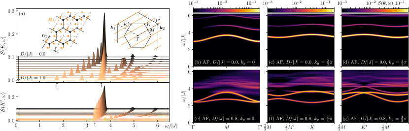
Figure 2: Dynamical spin-structure factor $\mathcal{S}(\bm{k},\omega)$ for the spin-$1/2$ honeycomb lattice antiferromagnet, $J_{z}/|J|=2.4$, and DMI obtained by numerically time-evolving a matrix product state [43]. (a) Line plots at the high-symmetry points $K$ (top) and $K^{\prime}$ (bottom) for increasing DMI from $D/|J|=0$ to $D/|J|=1$ illustrate the splitting of the spin-wave bands at $K$ while the splitting is absent at $K^{\prime}$. Magnon bands are highlighted by arrows. Insets show the lattice and the corresponding momenta lines determined by the cylindrical geometry with six sites circumference. (b-g) Representative color plots along aforementioned momenta cuts for zero DMI (top) and $D/|J|=0.8$ (bottom). The magnon bands (bright yellow features) split across the entire Brillouin zone apart from the $\Gamma$ and $K^{\prime}$ points that feature Dirac cones.

Model B1: Honeycomb Lattice Antiferromagnet.

As a first illustration of the problems faced by LSWT through the omission of longitudinal-transverse couplings (anisotropy blindness), we consider the honeycomb lattice spin-$1/2$ model with nearest neighbor Heisenberg coupling and interfacial Dzyaloshinskii-Moriya interaction (DMI), see inset in Fig. 2(a). The Hamiltonian is

$$H =\frac{1}{2}\sum_{\langle ij\rangle}\left[J_{z}S_{i}^{z}S_{j}^{z}+J\left(S_{i}^{x}S_{j}^{x}+S_{i}^{y}S_{j}^{y}\right)+\bm{D}_{ij}\cdot\bm{S}_{i}\times\bm{S}_{j}\right],$$ (1)

with $J_{z}>J>0$ being antiferromagnetic and $\bm{D}_{ij}=D\hat{\bm{z}}\times\hat{\bm{e}}_{ij}$; $\hat{\bm{e}}_{ij}$ is a unit vector along bond direction and $\hat{\bm{z}}$ along the lattice normal. For $J_{z}\gg J$ the strong easy-axis Ising anisotropy stabilizes the Néel ground state. The full model with group $\mathcal{G}_{M}$ has only discrete symmetries whereas the model without DMI has symmetry group $\mathcal{G}_{M}^{*}$ with a U(1) symmetry.

Expanding in fluctuations (sublattice-dependent bosons $a$ and $b$), one obtains the harmonic Hamiltonian in $\bm{k}$ space $H_{2}(J,J_{z})=\frac{1}{2}\sum_{\bm{k}}\bm{\psi}^{\dagger}_{\bm{k}}H_{\bm{k}}\bm{\psi}_{\bm{k}}$ featuring a block-diagonal kernel $H_{\bm{k}}=\mathrm{diag}(h_{\bm{k}},h_{-\bm{k}})$ in the basis $\bm{\psi}^{\dagger}_{\bm{k}}=(a^{\dagger}_{\bm{k}},b_{-\bm{k}},b^{\dagger}_{\bm{k}},a_{-\bm{k}})$ with

$$h_{\bm{k}}=\frac{1}{2}\begin{pmatrix}3J_{z}&-J\gamma_{\bm{k}}\\ -J\gamma_{-\bm{k}}&3J_{z}\end{pmatrix},\quad\gamma_{\bm{k}}=\sum_{n=0}^{2}\mathrm{e}^{\mathrm{i}\bm{k}\cdot\bm{\delta}_{n}}.$$ (2)

The nearest-neighbor bonds are $\bm{\delta}_{n}=(\cos\phi_{n},\sin\phi_{n})$ with $\phi_{n}=2\pi n/3+\pi/2$. After diagonalization, we find the normal mode magnon energies $\varepsilon_{\bm{k},\sigma}=\frac{1}{2}\sqrt{(3J_{z})^{2}-J^{2}|\gamma_{\bm{k}}|^{2}},$ which are two-fold spin-degenerate over the entire Brillouin zone ($\sigma=\uparrow,\downarrow$). This degeneracy is a result of the spurious U(1) and $PT$ symmetries in the LSWT. They appear because the harmonic theory is blind to the symmetry-breaking DMI which enters, to lowest order, to cubic order in the bosons. For a qualitative discussion of magnon-magnon interactions and their influence on the magnon spectrum see SM [48].

We explore the effects of the DMI by carrying out a real space perturbation theory [52], taking the Ising interaction as the unperturbed Hamiltonian and all other interactions as perturbations. Processes lifting the band degeneracy are found to second-order in the DMI-induced perturbation $V_{D}$ via virtual two-spin-flip states:

$$\frac{-2}{J_{z}}\left\langle\leavevmode\hbox to30.4pt{\vbox to17.74pt{\text{[drawing]}}}\right|V_{D}\left|\leavevmode\hbox to30.4pt{\vbox to17.74pt{\text{[drawing]}}}\right\rangle\left\langle\leavevmode\hbox to30.4pt{\vbox to17.74pt{\text{[drawing]}}}\right|V_{D}\left|\leavevmode\hbox to30.4pt{\vbox to17.74pt{\text{[drawing]}}}\right\rangle i j i j i j i j i j i j i j i j \propto\frac{D^{2}}{J_{z}}\mathrm{e}^{-2\mathrm{i}\varphi_{ij}},$$

where $\tan\varphi_{ij}=D_{ij}^{y}/D_{ij}^{x}$. The states depict the pattern of spin flips generated by $V_{D}$. White (black) circles indicate the ground state (spin flips). Such a coupling mimicks the bond-dependent symmetric off-diagonal exchange interaction that breaks spin conservation: $\mathrm{e}^{-2\mathrm{i}\varphi_{ij}}\frac{D^{2}}{J_{z}}S^{+}_{i}S^{+}_{j}$. Thus, by taking these terms to replace the DMI in Eq. (1), we account for the qualitative effects of DMI. We consider the amended Hamiltonian

$$H^{\prime}=\sum_{i\in\text{A}}\sum_{j=0}^{2} \left[J_{z}S_{i}^{z}S_{i+\bm{\delta}_{j}}^{z}+\frac{J}{2}\left(S_{i}^{+}S_{i+\bm{\delta}_{j}}^{-}+S_{i}^{-}S_{i+\bm{\delta}_{j}}^{+}\right)\right.$$

$$+\left.\frac{J_{++}^{\prime}}{2}\left(\mathrm{e}^{\mathrm{i}\vartheta_{\bm{\delta}_{j}}}S_{i}^{+}S_{i+\bm{\delta}_{j}}^{+}+\mathrm{e}^{-\mathrm{i}\vartheta_{\bm{\delta}_{j}}}S_{i}^{-}S_{i+\bm{\delta}_{j}}^{-}\right)\right],$$ (3)

where $|J_{++}^{\prime}|\propto D^{2}/J_{z}$. The $i$-sum runs over all sites of the A sublattice (spin-up) and the phases along the nearest-neighbor bonds read $\vartheta_{\bm{\delta}_{n}}=2\pi n/3$. A LSWT of $H^{\prime}$ yields a bilinear Hamiltonian $H^{\prime}_{2}(J,J_{z},D)$ that no longer features a block-diagonal kernel. As a result, the degeneracy of the magnon modes is lifted throughout the Brillouin zone except for the $\Gamma$ and the $K^{\prime}$ point, which feature magnon Dirac cones, in agreement with Refs. 53, 54; see the SM [48] for details.

The qualitative predictions of the modified LSWT are borne out by a fully nonperturbative calculation on the original model, Eq. (1). Figure 2 shows the dynamical spin-structure factor obtained from DMRG+tMPO; see SM for technical details [48]. Constant momentum slices show the progressive splitting of the bands at $K$ as a function of the DMI coupling [Fig. 2(a)]; in contrast, the magnon bands stay degenerate at $K^{\prime}$. As predicted, the DMI lifts the double degeneracy of the single magnon levels almost everywhere in the zone with exceptions at $\Gamma$ and $K^{\prime}$, where we find interaction-induced Dirac magnons [Figs. 2(b-g)].

Model B2: Honeycomb Lattice Ferromagnet.

A similar story holds for the ferromagnetic analogue of model B1. Within LSWT, the ferromagnet has two dispersive single magnon bands that meet at Dirac points at the $K$ and $K^{\prime}$ points, stabilized by a spurious time-reversal symmetry [15, 48] originating from a U(1) in the model without DMI (group $\mathcal{G}^{*}_{M}$). As before, the DMI breaks this spurious symmetry down to $\mathcal{G}_{M}$ but it does not enter the linear theory; however, it leads to topological magnon gaps via magnon-magnon interactions [15]. Here, we confirm these topological band gaps both via real space perturbation theory and nonperturbatively using DMRG+tMPO. Using real-space perturbation theory, we derive a modified LSWT that captures the topological gap opening by Haldane-type [55] second-neighbor hoppings [48]. The nonperturbative DMRG+tMPO data confirm that the Dirac cones are gapped out by the DMI (Fig. 3). Moreover, they show that the topological magnon modes are not dissolved into the continuum but rather are repelled by it (in line with general arguments in Ref. 56), pointing towards a considerably longer lifetime as expected from perturbation theory [15].

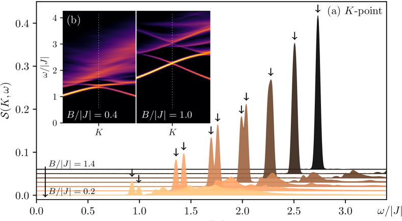
Figure 3: Numerically obtained dynamical spin-structure factors $\mathcal{S}(\bm{k},\omega)$ for the spin-$1/2$ honeycomb lattice ferromagnet with magnetic field, $B$, and DMI, $D/|J|=0.6$. (a) Line plots at the high-symmetry point $K$ illustrating the splitting of the Dirac-like mode in between the two magnon bands (highlighted by arrows). (b) Representative color plots of $\mathcal{S}(\bm{k},\omega)$ along a momenta cut including $K$, cf. inset of Fig. 2(a).

Model C: Tetragonal Lattice Model.

The previous examples are designed to understand in a simple way the mechanisms behind spurious LSWT symmetries. Here we show instead a non-fine-tuned 3D case, where the anisotropy blindness and shell anomaly join forces leading to enhanced symmetry in the LSWT (captured by magnetic group $\mathcal{G}_{E}^{*}$ of Fig. 1). As before, by going to further shells of interactions, the symmetry is lowered to that of the magnetic structure. We consider a ferromagnetic bipartite lattice with a tetragonal structure described by space group $P4$ [Fig. 4(a)]. This has low symmetry—with only a $C_{4}$ rotation around the $c$ (vertical) axis. For complete generality, we allow all the symmetry-allowed exchange terms within a shell. The minimal model that connects the moments in three dimensions includes both nearest and next-nearest neighbor couplings, with a total of $14$ possible exchange terms, or $10$ if we consider the anisotropy blindness (see also [48, 38]). We expect in this model, via representation theory, a Chern gap [38] which nevertheless is not present in LSWT in the $J_{1}+J_{2}$ model due to an enforced degenerate nodal line on the boundary of the Brillouin Zone [Fig. 4(b)] as shown in Fig. 4(c). The expected gap is recovered by going to the next shell—the $J_{1}+J_{2}+J_{3}$ model. The presence of this extra degeneracy can be understood in the context of spin-space group representation theory [48, 37]. The key spurious symmetry, present in the LSWT of $J_{1}+J_{2}$, is a glide plane, which is responsible for the nodal line degeneracy. This symmetry is allowed by anisotropy blindness which, in symmetry terms, amounts to a $C_{2}$ spin rotation around the $c$ axis. This two-fold spin rotation remains trivial for the $J_{1}+J_{2}+J_{3}$ model. But in the $J_{1}+J_{2}$ it combines with the remaining symmetries leading to an enhancement of the symmetries to a spin-space group.

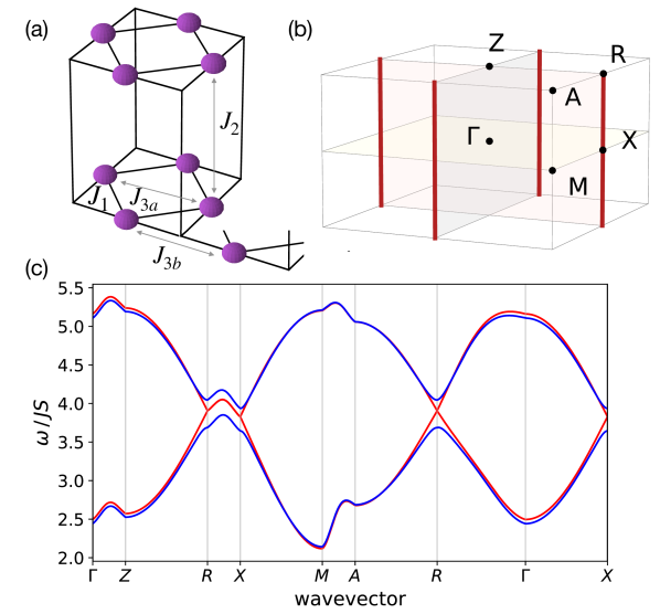
Figure 4: (a) Space group $P4$ tetragonal lattice and (b) corresponding Brillouin zone. Red lines indicate spurious nodal lines coming from the minimally coupled $J_{1}+J_{2}$ model in LSWT. (c) Magnon dispersions above the ferromagnetic ground state along high symmetry directions calculated within LSWT. The $J_{1}+J_{2}$ model (red) features spurious nodal lines, which are lifted switching on the next shell interaction $J_{3}$ (blue). The parameters are listed in the SM [48].

Discussion and symmetry context.

Consider the hypothetical situation where one wishes to characterise the magnetism of a material from spin wave data. As will be clear from the foregoing, the implementation of symmetries in LSWT contains potential pitfalls. We offer the following practical guide to using LSWT so that no spurious degeneracies arise.

Given a magnetic structure one may enumerate the spin and space locked transformations that leave the structure invariant. These symmetry elements form a magnetic space group $\mathcal{M}$. However, approximations to the full exchange Hamiltonian have the potential to break this locking leading to an enhanced symmetry formally described by spin-space groups [57, 58]. There may be physically well-motivated cases where the exchange couplings have spin-space symmetry—for example in collinear Heisenberg systems, in Kitaev magnets or generally when spin-orbit coupling is weak and there is a selection in the hierarchy of exchange terms [37]. There may be, in addition, cases where materials themselves realize a shell anomaly as a result of short-ranged couplings, leading to a physically relevant enhanced symmetry. This mechanism could be at work in MnF₂ (and possibly isostructural materials with weak spin-orbit coupling) [48, 44, 45, 50, 51]. Further high resolution experimental work may be of interest to look for degeneracy breaking in MnF₂.

However, as we have described, there are ways in which the intended symmetries may not be represented faithfully in the excitation spectrum. For example, one may underestimate the range of significant exchange couplings in the material leading to spurious symmetries at the Hamiltonian level. In the case of anisotropy blindness, Holstein-Primakoff LSWT itself has a spurious two-fold spin rotation symmetry around the magnetization vector for a collinear system that can lead to spin-space symmetries that are absent in the exact theory.

In general, as a practical rule of thumb, one should be especially cautious about LSWT for (i) collinear systems and for (ii) systems where the magnetic lattice has much higher symmetry than the entire crystal (model A, C), and, additionally, in the weak spin-orbit coupling regime when there are important couplings with longitudinal-transverse components (model B) [48]. To realize the correct symmetries in LSWT one should include all couplings consistent with the fundamental symmetries out to the $n$th shell until the spectrum ceases to change qualitatively. As an outlook, we emphasize that, where our discussion of the shell anomaly has focussed on its realization in spin waves, the ingredients to find it may arise in tight-binding models regardless of the quasiparticle type.

References

• Zhitomirsky and Chernyshev [2013] M. E. Zhitomirsky and A. L. Chernyshev, Colloquium: Spontaneous magnon decays, Rev. Mod. Phys. 85, 219 (2013).
• Malki and Uhrig [2020] M. Malki and G. Uhrig, Topological magnetic excitations, EPL (Europhysics Letters) 132, 20003 (2020).
• Bonbien et al. [2021] V. Bonbien, F. Zhuo, A. Salimath, O. Ly, A. Abbout, and A. Manchon, Topological aspects of antiferromagnets, Journal of Physics D: Applied Physics 55, 103002 (2021).
• McClarty [2022] P. A. McClarty, Topological magnons: A review, Annual Review of Condensed Matter Physics 13, 171 (2022).
• Chumak et al. [2015] A. V. Chumak, V. I. Vasyuchka, A. A. Serga, and B. Hillebrands, Magnon spintronics, Nature physics 11, 453 (2015).
• Holstein and Primakoff [1940] T. Holstein and H. Primakoff, Field dependence of the intrinsic domain magnetization of a ferromagnet, Phys. Rev. 58, 1098 (1940).
• Starykh et al. [2006] O. A. Starykh, A. V. Chubukov, and A. G. Abanov, Flat spin-wave dispersion in a triangular antiferromagnet, Phys. Rev. B 74, 180403(R) (2006).
• Chernyshev and Zhitomirsky [2009] A. L. Chernyshev and M. E. Zhitomirsky, Spin waves in a triangular lattice antiferromagnet: Decays, spectrum renormalization, and singularities, Phys. Rev. B 79, 144416 (2009).
• Sachdev [2011] S. Sachdev, Quantum phase transitions (Cambridge university press, 2011).
• Villain et al. [1980] J. Villain, R. Bidaux, J.-P. Carton, and R. Conte, Order as an effect of disorder, Journal de Physique 41, 1263 (1980).
• Shender [1982] E. Shender, Antiferromagnetic garnets with fluctuationally interacting sublattices, Soviet Journal of Experimental and Theoretical Physics 56, 178 (1982).
• Henley [1989] C. L. Henley, Ordering due to disorder in a frustrated vector antiferromagnet, Phys. Rev. Lett. 62, 2056 (1989).
• Chalker et al. [1992] J. T. Chalker, P. C. W. Holdsworth, and E. F. Shender, Hidden order in a frustrated system: Properties of the heisenberg kagomé antiferromagnet, Phys. Rev. Lett. 68, 855 (1992).
• Rau et al. [2018] J. G. Rau, P. A. McClarty, and R. Moessner, Pseudo-goldstone gaps and order-by-quantum disorder in frustrated magnets, Phys. Rev. Lett. 121, 237201 (2018).
• Mook et al. [2021a] A. Mook, K. Plekhanov, J. Klinovaja, and D. Loss, Interaction-stabilized topological magnon insulator in ferromagnets, Phys. Rev. X 11, 021061 (2021a).
• Katsura et al. [2010] H. Katsura, N. Nagaosa, and P. A. Lee, Theory of the thermal hall effect in quantum magnets, Phys. Rev. Lett. 104, 066403 (2010).
• Onose et al. [2010] Y. Onose, T. Ideue, H. Katsura, Y. Shiomi, N. Nagaosa, and Y. Tokura, Observation of the magnon hall effect, Science 329, 297 (2010).
• Ideue et al. [2012] T. Ideue, Y. Onose, H. Katsura, Y. Shiomi, S. Ishiwata, N. Nagaosa, and Y. Tokura, Effect of lattice geometry on magnon hall effect in ferromagnetic insulators, Phys. Rev. B 85, 134411 (2012).
• Zhang et al. [2013] L. Zhang, J. Ren, J.-S. Wang, and B. Li, Topological magnon insulator in insulating ferromagnet, Phys. Rev. B 87, 144101 (2013).
• van Hoogdalem et al. [2013] K. A. van Hoogdalem, Y. Tserkovnyak, and D. Loss, Magnetic texture-induced thermal hall effects, Phys. Rev. B 87, 024402 (2013).
• Shindou et al. [2013a] R. Shindou, R. Matsumoto, S. Murakami, and J.-i. Ohe, Topological chiral magnonic edge mode in a magnonic crystal, Phys. Rev. B 87, 174427 (2013a).
• Shindou et al. [2013b] R. Shindou, J.-i. Ohe, R. Matsumoto, S. Murakami, and E. Saitoh, Chiral spin-wave edge modes in dipolar magnetic thin films, Phys. Rev. B 87, 174402 (2013b).
• Shindou and Ohe [2014] R. Shindou and J.-i. Ohe, Magnetostatic wave analog of integer quantum hall state in patterned magnetic films, Phys. Rev. B 89, 054412 (2014).
• Mook et al. [2014a] A. Mook, J. Henk, and I. Mertig, Magnon hall effect and topology in kagome lattices: A theoretical investigation, Phys. Rev. B 89, 134409 (2014a).
• Mook et al. [2014b] A. Mook, J. Henk, and I. Mertig, Edge states in topological magnon insulators, Phys. Rev. B 90, 024412 (2014b).
• Owerre [2016] S. A. Owerre, A first theoretical realization of honeycomb topological magnon insulator, Journal of Physics: Condensed Matter 28, 386001 (2016).
• Chisnell et al. [2015] R. Chisnell, J. S. Helton, D. E. Freedman, D. K. Singh, R. I. Bewley, D. G. Nocera, and Y. S. Lee, Topological magnon bands in a kagome lattice ferromagnet, Phys. Rev. Lett. 115, 147201 (2015).
• Chen et al. [2018a] L. Chen, J.-H. Chung, B. Gao, T. Chen, M. B. Stone, A. I. Kolesnikov, Q. Huang, and P. Dai, Topological spin excitations in honeycomb ferromagnet ${\mathrm{CrI}}_{3}$Phys. Rev. X 8, 041028 (2018a).
• Fransson et al. [2016] J. Fransson, A. M. Black-Schaffer, and A. V. Balatsky, Magnon Dirac materials, Phys. Rev. B 94, 075401 (2016).
• Mook et al. [2016] A. Mook, J. Henk, and I. Mertig, Tunable magnon weyl points in ferromagnetic pyrochlores, Phys. Rev. Lett. 117, 157204 (2016).
• Xu et al. [2016] B. Xu, T. Ohtsuki, and R. Shindou, Integer quantum magnon hall plateau-plateau transition in a spin-ice model, Phys. Rev. B 94, 220403(R) (2016).
• McClarty et al. [2018] P. A. McClarty, X.-Y. Dong, M. Gohlke, J. G. Rau, F. Pollmann, R. Moessner, and K. Penc, Topological magnons in Kitaev magnets at high fields, Phys. Rev. B 98, 060404(R) (2018).
• Chen et al. [2018b] L. Chen, J.-H. Chung, B. Gao, T. Chen, M. B. Stone, A. I. Kolesnikov, Q. Huang, and P. Dai, Topological spin excitations in honeycomb ferromagnet ${\mathrm{cri}}_{3}$Phys. Rev. X 8, 041028 (2018b).
• Yuan et al. [2020] B. Yuan, I. Khait, G.-J. Shu, F. C. Chou, M. B. Stone, J. P. Clancy, A. Paramekanti, and Y.-J. Kim, Dirac magnons in a honeycomb lattice quantum $\mathit{XY}$ magnet ${\mathrm{CoTiO}}_{3}$Phys. Rev. X 10, 011062 (2020).
• Mook et al. [2021b] A. Mook, S. A. Díaz, J. Klinovaja, and D. Loss, Chiral hinge magnons in second-order topological magnon insulators, Phys. Rev. B 104, 024406 (2021b).
• Scheie et al. [2022] A. Scheie, P. Laurell, P. A. McClarty, G. E. Granroth, M. B. Stone, R. Moessner, and S. E. Nagler, Dirac magnons, nodal lines, and nodal plane in elemental gadolinium, Phys. Rev. Lett. 128, 097201 (2022).
• Corticelli et al. [2022a] A. Corticelli, R. Moessner, and P. A. McClarty, Spin-space groups and magnon band topology, Phys. Rev. B 105, 064430 (2022a).
• Corticelli et al. [2022b] A. Corticelli, R. Moessner, and P. A. McClarty, Identifying, and constructing, complex magnon band topology, arXiv:2203.06678 (2022b).
• Lin et al. [1998] H.-H. Lin, L. Balents, and M. P. A. Fisher, Exact so(8) symmetry in the weakly-interacting two-leg ladder, Phys. Rev. B 58, 1794 (1998).
• James et al. [2018] A. J. A. James, R. M. Konik, P. Lecheminant, N. J. Robinson, and A. M. Tsvelik, Non-perturbative methodologies for low-dimensional strongly-correlated systems: From non-abelian bosonization to truncated spectrum methods, Reports on Progress in Physics 81, 046002 (2018).
• White [1992] S. R. White, Density matrix formulation for quantum renormalization groups, Phys. Rev. Lett. 69, 2863 (1992).
• Phien et al. [2012] H. N. Phien, G. Vidal, and I. P. McCulloch, Infinite boundary conditions for matrix product state calculations, Phys. Rev. B 86, 245107 (2012).
• Zaletel et al. [2015] M. P. Zaletel, R. S. K. Mong, C. Karrasch, J. E. Moore, and F. Pollmann, Time-evolving a matrix product state with long-ranged interactions, Phys. Rev. B 91, 165112 (2015).
• Šmejkal et al. [2022] L. Šmejkal, J. Sinova, and T. Jungwirth, Beyond conventional ferromagnetism and antiferromagnetism: A phase with nonrelativistic spin and crystal rotation symmetry, Phys. Rev. X 12, 031042 (2022).
• Šmejkal et al. [2022] L. Šmejkal, J. Sinova, and T. Jungwirth, Emerging research landscape of altermagnetism, arXiv e-prints , arXiv:2204.10844 (2022), arXiv:2204.10844 [cond-mat.mes-hall] .
• Garst et al. [2017] M. Garst, J. Waizner, and D. Grundler, Collective spin excitations of helices and magnetic skyrmions: review and perspectives of magnonics in non-centrosymmetric magnets, Journal of Physics D: Applied Physics 50, 293002 (2017).
• Burch et al. [2018] K. S. Burch, D. Mandrus, and J.-G. Park, Magnetism in two-dimensional van der waals materials, Nature 563, 47 (2018).
• [48] The Supplemental Material at [URL inserted by publisher] contains Refs. 59, 60, 61, 62, 63, 64, 65, 66, 67, 68 and further details and additional supporting data.
• Naka et al. [2019] M. Naka, S. Hayami, H. Kusunose, Y. Yanagi, Y. Motome, and H. Seo, Spin current generation in organic antiferromagnets, Nature Communications 1010.1038/s41467-019-12229-y (2019).
• Nikotin et al. [1969] O. Nikotin, P. A. Lindgård, and O. W. Dietrich, Magnon dispersion relation and exchange interactions in MnF2, Journal of Physics C: Solid State Physics 2, 1168 (1969).
• Hutchings et al. [1970] M. T. Hutchings, B. D. Rainford, and H. J. Guggenheim, Spin waves in antiferromagnetic FeF2Journal of Physics C Solid State Physics 3, 307 (1970).
• Zhitomirsky [2015] M. E. Zhitomirsky, Real-space perturbation theory for frustrated magnets: application to magnetization plateaus, Journal of Physics: Conference Series 592, 012110 (2015).
• Matsumoto and Hayami [2020] T. Matsumoto and S. Hayami, Nonreciprocal magnons due to symmetric anisotropic exchange interaction in honeycomb antiferromagnets, Phys. Rev. B 101, 224419 (2020).
• Neumann et al. [2022] R. R. Neumann, A. Mook, J. Henk, and I. Mertig, Thermal hall effect of magnons in collinear antiferromagnetic insulators: Signatures of magnetic and topological phase transitions, Phys. Rev. Lett. 128, 117201 (2022).
• Haldane [1988] F. D. M. Haldane, Model for a quantum hall effect without landau levels: Condensed-matter realization of the "parity anomaly", Phys. Rev. Lett. 61, 2015 (1988).
• Verresen et al. [2019] R. Verresen, R. Moessner, and F. Pollmann, Avoided quasiparticle decay from strong quantum interactions, Nature Physics 15, 750 (2019).
• Brinkman and Elliott [1966] W. F. Brinkman and R. J. Elliott, Theory of Spin-Space Groups, Proceedings of the Royal Society of London Series A 294, 343 (1966).
• Litvin and Opechowski [1974] D. B. Litvin and W. Opechowski, Spin groups, Physica 76, 538 (1974).
• Harris et al. [1971] A. B. Harris, D. Kumar, B. I. Halperin, and P. C. Hohenberg, Dynamics of an antiferromagnet at low temperatures: Spin-wave damping and hydrodynamics, Phys. Rev. B 3, 961 (1971).
• Cohen-Tannoudji et al. [1998] C. Cohen-Tannoudji, J. Dupont-Roc, and G. Grynberg, Atom—Photon Interactions (Wiley, 1998).
• McCulloch [2008] I. P. McCulloch, Infinite size density matrix renormalization group, revisited, arXiv:0804.2509 (2008).
• Gendiar et al. [2009] A. Gendiar, R. Krcmar, and T. Nishino, Spherical Deformation for One-Dimensional Quantum Systems, Progress of Theoretical Physics 122, 953 (2009).
• Yule [1927] G. U. Yule, VII. On a method of investigating periodicities disturbed series, with special reference to Wolfer’s sunspot numbers, Philos. Trans. R. Soc. London, Ser. A 226, 267 (1927).
• Makhoul [1975] J. Makhoul, Linear prediction: A tutorial review, Proceedings of the IEEE 63, 561 (1975).
• Barthel et al. [2009] T. Barthel, U. Schollwöck, and S. R. White, Spectral functions in one-dimensional quantum systems at finite temperature using the density matrix renormalization group, Phys. Rev. B 79, 245101 (2009).
• Mühlbauer et al. [2009] S. Mühlbauer, B. Binz, F. Jonietz, C. Pfleiderer, A. Rosch, A. Neubauer, R. Georgii, and P. Böni, Skyrmion lattice in a chiral magnet, Science 323, 915 (2009).
• Han et al. [2010] J. H. Han, J. Zang, Z. Yang, J.-H. Park, and N. Nagaosa, Skyrmion lattice in a two-dimensional chiral magnet, Phys. Rev. B 82, 094429 (2010).
• Bradley and Cracknell [2009] C. Bradley and A. Cracknell, The mathematical theory of symmetry in solids (Oxford University Press, 2009).