Homogeneous nucleation of dislocations as a pattern formation phenomenon

Abstract

Dislocation nucleation in homogeneous crystals initially unfolds as a linear symmetry-breaking elastic instability. In the absence of explicit nucleation centers, such instability develops simultaneously all over the crystal and due to the dominance of long range elastic interactions it advances into the nonlinear stage as a collective phenomenon through pattern formation. In this paper we use a novel mesoscopic tensorial model (MTM) of crystal plasticity to study the delicate role of crystallographic symmetry in the development of the dislocation nucleation patterns in defect free crystals loaded in a hard device. The model is formulated in 2D and we systematically compare lattices with square and triangular symmetry. To avoid the prevalence of the conventional plastic mechanisms, we consider the loading paths represented by pure shears applied on the boundary of the otherwise unloaded body. These loading protocols can be qualified as exploiting the ’softest’ and the ’hardest’ directions and we show that the associated dislocation patterns are strikingly different.

1 Introduction

Plastic flow in crystals is a result of the motion of crystal defects among which the dominant role is played by lattice dislocations [1, 2, 3, 4, 5]. Understanding the mechanism of creation of dislocations is essential for the development of the fundamental theory of crystal plasticity allowing one to control the mechanical strength of crystalline materials [6, 7, 8, 9].

Homogeneous nucleation of dislocations in crystalline solids attracts particular attention as the main mechanism for incipient plasticity in nanomaterials where one usually has to deal with practically defect-free crystals [10, 11, 12, 13]. Since the action of standard (heterogeneous) dislocation sources at these scales is suppressed, the knowledge of alternative (homogeneous) dislocation nucleation mechanisms is of crucial importance for the understanding of the response of such materials which are known to demonstrate extraordinary mechanical properties due to the presence of peculiar, micro-scale-specific deformation mechanisms [14, 15, 16].

Nucleation of dislocations signals the loss of stability of a perfect lattice subjected to sufficiently large shear stresses [17]. The resulting symmetry breaking instability may lead to reconfiguration of only few atomic bonds, as is the case of a nucleation of a single dislocation, or carry a large-scale restructuring of the atomic lattice, as during a catastrophic, brittle-like, collective nucleation of a large number of dislocations which leads to the formation of intricate dislocation patterns [18]. Although at macro-scales such massive nucleation of dislocations can be usually neglected in comparison with emission of individual dislocations from heterogeneities, it may be also a dominant factor in bulk materials subjected to high intensity dynamic loadings [19, 20].

Given that the sizes associated with dislocation cores can be as small as a few lattice spacings, the continuum theory is hardly applicable for the description of the developed (post-bifurcational) stages of lattice instability resulting in the formation of dislocations. Therefore molecular dynamics simulation played an important role in uncovering the fundamental mechanisms of the nucleation of individual dislocations, however its limited timescale still remains a significant challenge for studying collective nucleation at experimentally relevant conditions [21]. Therefore various accelerated meso-scale approaches have been used including the microscopic phase-field crystal theory [22, 23], the multi-scale quasi-continuum method [24], the periodized-discrete-elasticity model [25], and the phase-field dislocation dynamics [26]. Each of these conceptual and computational approaches was successful in addressing a particular range of time and length scales.

Major efforts have been focused on finding the dislocation nucleation criterion [27, 28, 29]. Given that behind dislocation nucleation is a linear instability of an elastically pre-stressed solid, many attempts were made to reduce the corresponding continuum-scale criterion to nanoscale, for instance, by using the continuum loss of strong ellipticity condition with atomic level entries [30, 31]. However, even in the case of apparently homogeneous dislocation nucleation under micro-indenter, the molecular dynamics simulations revealed complex mesoscale processes involving a large number of atoms and producing a strong local distortion of the lattice which makes a phonon stability analysis hardly applicable [32, 33, 34, 35]. As a result various nonlocal corrections were proposed to ’delocalize’ the mesoscale atomic acoustic tensor and the results were extensively compared with molecular dynamics simulations [36]. Despite this progress, our ability to predict the instant and the location of the nucleation of an individual dislocation remains limited, while the first efforts to understand the corresponding collective effects have started only recently [37, 18]. Moreover, little remains known about the collective side of dislocation nucleation including the dependence of emerging patterns of cells and walls on the crystallographic symmetry of the lattice.

The goal of this paper is to contribute to the understanding of the collective nucleation of dislocations in perfect crystals as a bifurcation phenomenon with the focus on post-bifurcational development of patterns and textures. We assume that in the absence of explicit nucleation centers, the implied instability develops simultaneously all over the crystal and that, due to the dominance of long range elastic interactions, it proceeds into the nonlinear stage as a cooperative avalanche which involves self-organization of dislocations into energy minimizing patterns. We design a series of numerical experiments where we load pristine crystals with different crystallographic symmetries beyond the stability limit of the homogeneous state and then study the transient unfolding of the dislocation nucleation avalanche which leads to the catastrophic stress drop as the optimal dislocational microstructure settles down. For simplicity we operate in 2D where we can systematically compare the peculiarities of the collective nucleation in lattices with square and triangular symmetry. To avoid immediate activation of the conventional plastic mechanisms, we consider the loading paths represented by pure shears applied on the boundary of the otherwise unloaded body. These loading protocols can be qualified as exploiting the ’softest’ and the ’hardest’ directions and we show that the associated dislocation patterns are strikingly different.

Our main computational tool is the novel mesoscopic tensorial model (MTM) of crystal plasticity allowing one to capture in a geometrically precise way the role of crystallographically-specific lattice invariant shears while still operating with the macroscopic notions of stress and strain [38, 39, 37, 40, 18, 41]. The model implies the construction of an energy density respecting the global symmetry of Bravais lattices described by the group $GL(n,\mathbb{Z})$ [42, 43, 44, 45, 46].

The resulting theory can be viewed as a finite element version of nonlinear elasticity theory accounting for geometrically nonlinear kinematics. The size of the elements is viewed as a physical regularizing (cut-off) parameter bringing an internal scale into the theory. Behind such coarse-grained approach lies the assumption that the deformation inside the meso-scale material elements can be considered as affine and their response is characterized by an effective energy landscape which is globally periodic due to the presence of an infinite number of equivalent lattice configurations. From the perspective of such Landau-type continuum theory, plastically deformed crystal can be seen as a multi-phase mixture of equivalent “phases”. Plastic yield can be then interpreted as an escape from the reference energy well, and plastic “mechanisms” can be linked to low-barrier valleys of the energy landscape. Rate-independent dissipation emerges in such theory due to the fast (abrupt, at the time scale of the loading) well-switching events describing elementary plastic slips.

The main advantage of the MTM approach is that it is formulated in terms of macroscopically measurable quantities (stress and strain) while being able to distinguish between different crystal symmetries including the resolution of the symmetry dependent configuration of the dislocation cores. It can therefore account adequately for both long- and short-range interactions between dislocations. Most importantly, it allows for topological transitions associated with dislocation nucleation and annihilation even though the details of the corresponding “reactions” may appear as blurred on the scale of regularization. Last but not least, in the MTM approach the interaction of dislocations with various obstacles, including self locking and the formation of other types of dislocational entanglements can be handled without introducing ad-hoc relations.

Using this modeling framework we show that following the loss of elastic stability plasticity develops in the form of a system size avalanche which involves massive nucleation of dislocations which self-organize into system size patterns. The latter involves the formation of extended low-energy patches (or grains) undergoing pseudo-rigid rotations. Individual grains are separated by high-energy dislocation walls. The observed deformation patterns defy conventional continuum description with its insistence on rigid plastic mechanisms limited to crystallographically specific simple shears and the neglect of the effects of geometrical nonlinearity. More complex picture is observed with various slip systems activated simultaneously and finite elasticity playing an important role in the observed dislocation patterning.

The fact that the MTM energy can be formulated for lattices with different symmetries and that we can model general loading paths allows us to explore non-trivial deformation mechanisms peculiar to lattices with higher and lower symmetries. To highlight these ideas we focus in what follows on the simplest nontrivial case of 2D lattices with two types of symmetries, square and triangular. We study systematically two fundamentally different loading directions which we consider as providing conceptual bounds for the whole spectrum of available responses. One of them is directed towards the lowest and another one to the highest energy barrier away from the original energy well. The resulting breakdown of the original homogeneous state displays complex nucleation pattern with a large number of nucleated dislocations forming a highly organized crystal texture. The ’softest’ path highlights the role of the metastable phases in driving the complexity of the emerging dislocation arrangement. The ’hardest’ path shows in some cases the possibility of collective rearrangements of the lattice taking the form of inelastic rotations in which dislocations play the role of invisible intermediaries.

The paper is organized as follows. We begin by introducing the $GL(2,\mathbb{Z})$-invariant energy and discuss the resulting energy landscape (Section 2). In Section 3, we propose the criterion detecting the instability of the homogeneously loaded lattice which reveals various features of the activated instability modes. We then present in Section 4 the results of the numerical experiments which confirm the validity of our instability criterion and show the post avalanche arrangement of the nucleated dislocations. A brief description of the numerical method is given in the Appendix. Our conclusions are summarized in the final Section 5.

2 The model

Lattice invariant shears.

The proposed model, whose simplest nontrivial formulation is for 2D Bravais lattices which are solely considered in this paper, allows one to include plastic deformation in a continuum elastic framework, while simultaneously accounting of the discrete nature of the underlying lattice structure. This is achieved with the construction of an energy density whose material symmetry properties are described by the global symmetry group of the lattice $GL(2,\mathbb{Z})$. The latter is broader than the crystallographic point group [47] and includes the lattice invariant shears accounting for plastic slips [48, 49, 50, 51, 52, 53].

The energy density in the MTM model should be invariant of the action of the group $GL(2,\mathbb{Z})$ which is comprised of unimodular integer valued matrices $\mathbf{m}$. Indeed, two basis ${\bf e}_{I}$ and ${\bar{\bf e}}_{I}$ describe the same lattice if and only if [54]: ${\bf{e}}_{J}=m_{IJ}\bar{\bf e}_{I}\;\;\mbox{with}\;\;{m}_{IJ}\in{\mathbb{Z}}.$ Then, we can say that all 2D simple lattices are invariant under the action of a group $GL(2,\mathbb{Z})=\left\{{\bf m},\,m_{IJ}\in{\mathbb{Z}},\,\det(\bf m)=\pm 1\right\}.$ The fact that this matrices are unimodular (i.e. $\det{\bf m}=\pm 1$) reflects the condition that these transformations do no affect the volume of the lattice cell (the case $\det{\bf m}=-1$ corresponds to reflection). We remark that the group $GL(2,\mathbb{Z})$ accounts for the lattice invariance in shear, but also of invariance under rotations and reflections and in this sense the group $GL(2,\mathbb{Z})$ constitutes the finite strain extension of the crystallographic point group [55]. Every time we multiply a lattice basis with a matrix $\mathbf{m}\in GL(2,\mathbb{Z})$, we obtain a crystallographically-equivalent structure with exactly the same energy. The resulting multiplicity of the energy wells implies that such equivalent configurations can be interpreted as different ”phases” describing the same crystal. In such a description, dislocations will appear as incompatible parts of the resulting ’phase boundaries’.

In the following we take for granted that the lattice energy density $\varphi\left(\bar{\mathbf{e}}_{i}\right)$, where $\bar{\mathbf{e}}_{i}=\mathbf{F}\mathbf{e}^{0}_{i}$ is the deformed basis while $\mathbf{e}^{0}_{i}$ is the reference basis, can be identified with a continuum strain energy density such that $\phi(\mathbf{F}):=\varphi(\mathbf{F}\mathbf{e}^{0})$, with $\mathbf{F}=\nabla\mathbf{u}$ the deformation gradient. In view of frame indifference requirement, the strain energy density $\phi$ must be a function of the lattice metric tensor ${\bf C}={\bf F}^{T}{\bf F}$ [56, 57]. The configuration space is then described by the three significant components of the metric tensor: $C_{11},C_{22}$ and $C_{12}$. Every point of the surface $\det{\bf C}=C_{22}C_{11}-C^{2}_{12}=1$ corresponds to an orbit represented by rigidly rotated lattice configurations.

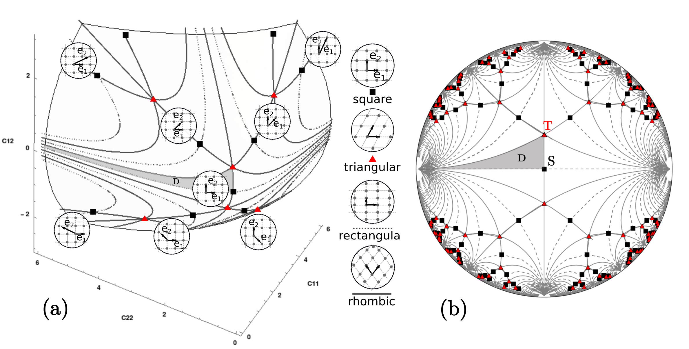
Figure 1: (a) A portion of the hyperbolic surface $\det{\bf C}=1$, points and lines corresponds to the different Bravais lattices. The respective basis vectors ${\bf e}_{i}$ are shown on insets. (b) A stereographic projection of the surface $\det{\bf C}=1$ on the Poincare disk. $D$ is the minimal periodicity domain.

Minimum periodic domain.

The global invariance of the energy suggests that we can construct the image of ${\bf C}$ in the minimum periodicity domain $D=\{C\in\det{\bf C}=1,\quad 0<C_{11}\leq C_{22},\quad 0\leq C_{12}\leq C_{11}/2\}.$ The metric tensors belonging to it are associated with lattices basis characterized by the ”minimal” vectors $\tilde{\mathbf{e}}_{1},\tilde{\mathbf{e}}_{2}$, because they are selected in such a way that: $\tilde{\mathbf{e}}_{1}$ is the shortest lattice vector and $\tilde{\mathbf{e}}_{2}$ is the shortest lattice vector not collinear with $\tilde{\mathbf{e}}_{1}$ and for which the sign is chosen in such a way that the angle between the two is acute. This type of basis is said to have reduced form of Lagrange [58].

To better visualize the tessellation of the configurational space into equivalent periodicity domains, we will use in what follows the stereographic projection of the infinite surface $\det{\bf C}=1$ on a disk with unit radius (Poincaré disk). The mapping, which associates the configuration $(C_{11},C_{22},C_{12})$ with the point $(x,y)$ on the unit disk, is given by the formulas

$$x=\frac{(\frac{C_{12}}{C_{22}})^{2}+(\frac{\sqrt{\det\bf C}}{C_{22}})^{2}-1}{(\frac{C_{12}}{C_{22}})^{2}+((\frac{\sqrt{\det\bf C}}{C_{22}})+1)^{2}},\,\,y=\frac{2(\frac{C_{12}}{C_{22}})}{(\frac{C_{12}}{C_{22}})^{2}+((\frac{\sqrt{\det\bf C}}{C_{22}})+1)^{2}}.$$ (1)

In Fig. 1 we show the location of the minimal periodicity domain $D$ on the hyperbolic surface $\det{\bf C}=1$ in the space of metric tensors and on its projection on the Poincaré disk. We highlight there the configurations $\bf S$ and $\bf T$ which are the unique representatives of the infinite equivalence classes of unloaded square and triangular lattices, belonging to $D$. The small black squares in Fig. 1 corresponding to other (not belonging to $D$) variants of the square lattice, while the other equivalent variants of triangular lattices with hexagonal symmetry are represented by small red triangles. The rectangular and the rhombic lattices with one parametric degeneracy are also located in Fig. 1 along the continuous and dashed grey lines; the generic obliques lattices with two parametric degeneracy are located in the open regions of the configuration.

Lagrange reduction.

For the ’equivalent’ of ${\bf C}$ inside the minimal periodicity domain we use the notation ${\bf C^{0}}$. The metric tensor ${\bf C^{0}}$ is defined by the mapping ${\bf C}^{0}={\bf m}^{T}{\bf C}{\bf m}$. The task of finding the corresponding unimodular matrix ${\bf m}$ is known as the Lagrange reduction [58]. It is a recursive procedure which can be formulated in the form of an algorithm [58]: (i) initiate ${\bf m}=\mathbb{I}$; (ii) define the following three matrices : ${\bf m}_{1}=\begin{pmatrix}1&0\\ 0&-1\end{pmatrix}$, ${\bf m}_{2}=\begin{pmatrix}0&1\\ 1&0\end{pmatrix}$, ${\bf m}_{3}=\begin{pmatrix}1&-1\\ 0&1\end{pmatrix}$; (iii) initiate recursive algorithm : (iv) if $C_{12}<0$, change sign to $C_{12}$, ${\bf m}\rightarrow$m${\bf m}_{1}$; (v) if $C_{22}<C_{11}$, swap these two components, ${\bf m}\rightarrow$m${\bf m}_{2}$; (vi) if $2C_{12}>C_{11}$, set $C_{12}=C_{12}-C_{11}$, and $C_{22}=C_{22}+C_{11}-2C_{12}$, ${\bf m}\rightarrow$m${\bf m}_{3}$. Note that the action of the matrix ${\bf m}_{1}$ is related to the sign of the angle between two lattice vectors $\mathbf{e}_{i}$ and returns an acute angle, whereas the action of the matrix ${\bf m}_{2}$ is to swap two lattice vectors $\mathbf{e}_{i}$. Therefore, both these two operations do not result in any change in vectors’ length and effectively propagate the metric in the same elastic well composed of the four copies of the fundamental domain $D$ and therefore are not associated with a plastic strain. On the other hand, the length of the lattice vectors is changed (shortened) under the action of the matrix ${\bf m}_{3}$, which indicates that the current metric belongs to another elastic well and accumulates plastic strain.

Energy density.

Given that the energy density will be defined fully as long as it is defined in the minimum periodicity domain and we will use for such a single period description a special notation $\phi_{D}(\bf C^{0})$ so that $\phi({\bf C})=\phi({\bf m}^{T}{\bf C}{\bf m})=\phi_{D}(\bf C^{0}).$ By defining $\phi_{D}$ as a function of scaled variables $\tilde{\bf C}={\bf C}/({\det^{1/2}\bf C})$ we decouple the isochoric contribution to the energy from the volumetric one that can be added separately. We will require $\phi_{D}$ to satisfy $\mathcal{C}^{2}$ smoothness, which ensures the continuity of the elastic moduli. Moreover, $\phi_{D}$ must have a minimum which corresponds to the chosen crystal symmetry. For instance, when modelling a square lattice, $\phi_{D}$ will be constructed in such a way that minimum coincides with the square symmetry lattice (that is point $C_{11}=C_{22}=1$, $C_{12}=0$).

A general $6$-th order polynomial energy $\phi_{D}$ with the required properties was introduced in [46]. The energy density is written in terms of the three invariants: $I_{1}=\frac{1}{3}(C_{11}+C_{22}-C_{12})$, $I_{2}=\frac{1}{4}(C_{11}-C_{22})^{2}+\frac{1}{12}(C_{11}+C_{22}-4C_{12})^{2}$ and $I_{3}=(C_{11}-C_{22})^{2}(C_{11}+C_{22}-4C_{12})-\frac{1}{9}(C_{11}+C_{22}-4C_{12})^{3}$ and can be written as $\tilde{\phi}_{D}(\tilde{\bf C})=\beta_{1}\psi_{1}(\tilde{\bf C})+\psi_{3}(\tilde{\bf C})$ where $\psi_{1}={I_{1}}^{4}\,I_{2}-\frac{41\,{I_{2}}^{3}}{99}+\frac{7\,I_{1}\,I_{2}\,I_{3}}{66}+\frac{{I_{3}}sof^{2}}{1056}$ and $\psi_{2}=\frac{4\,{I_{2}}^{3}}{11}+{I_{1}}^{3}\,I_{3}-\frac{8\,I_{1}\,I_{2}\,I_{3}}{11}+\frac{17\,{I_{3}}^{2}}{528}.$ The value of parameter $\beta_{1}=-0.25$ ($\beta_{1}=4$) must be set to ensure that the global minimum of the energy corresponds to square (triangular) symmetry. The proposed energy $\tilde{\phi}_{D}(\tilde{\bf C})$ concerns metrics located on the surface $\det{\bf C}=1$. To account for configurations which also allows for a volume change, we can add a volumetric term to $\tilde{\phi}_{D}(\tilde{\bf C})$. For instance, to exclude configurations with infinite compression one can use an expression $h(\det{\bf C})=-K(\ln\det{\bf C}-\det{\bf C}),$ so that $\phi_{D}({\bf C})=\tilde{\phi}_{D}(\tilde{\bf C})+h(\det{\bf C})$ where the coefficient K plays the role of a bulk modulus. The energy density $\phi_{D}({\bf C})$ is used in all numerical experiments reported in this paper.

Internal length scale.

Since the energy $\phi$ is non convex, the corresponding continuum elasticity problem, which is by definition scale free, is highly degenerate. The minimization in this setting can produce infinitely fine microstructures [59] reducing the stiffness in the relaxed problem to zero [60]. This lack of convexity is a property that the MTM of crystal plasticity shares with other similar Landau type theories. However, in contrast to the conventional Ginzburg-Landau approaches, relying for regularization on higher gradients of the order parameters, in MTM the regularization is achieved by spatial discretization, which reduces the space of admissible deformations to a finite dimensional set of compatible, piece-wise affine mappings. In other words, deformation is assumed to be piecewise linear and the elastic response is attributed to discrete material elements whose scale $h$ defines the resolution of the model (meso-scale) and is viewed as a physical parameter [38, 37].

More specifically, the original lattice is coarse grained with an introduction of a uniform meso-scale grid reproducing the symmetry of the crystal. The scale of the elements of the grid is selected to make sure that the Cauchy-Born type energy [53, 61], computed by ab initio methods for elements in the corresponding range of sizes, is essentially periodic in the interesting range of strains. In many crystals the periodicity at the level of the few first energy wells can be captured already for $h\sim 10a$ where $a$ is the atomic scale. In the resulting coarse grained description, some microscopic features like, for instance, dislocation cores will emerge as blurred because the scales smaller than $h$ are effectively homogenized out. While some aspects of a truly atomistic description will be then necessarily lost, for instance, the implied cut-offs may compromise the short-range interaction of dislocation cores during dislocation reactions, the crucial meso-scopic interactions at distances of the order and larger than $h$ are expected to be captured correctly. If we normalize the linear size of the macroscopic sample by setting $L=1$, we acquire a small dimensionless parameter $h/L=1/N$, where $N^{2}$ is the number of the nodes in the mesoscopic finite-element grid. For instance, if $h$ is in $nm$ size range, the simulations with $N\sim 10^{3}$ would describe a micrometer size samples.

Computational approach.

Solution of a continuum elastic problem implies local minimization of the energy $W=\int_{\Omega}\phi(\nabla\mathbb{y})d\mathbb{x}$ which is prescribed on a reference domain $\Omega$. We assume that the system is loaded by an affine displacement field prescribed on $\partial\Omega$ (hard device). The conditions of mechanical equilibrium read $\nabla\cdot\mathbf{P}=0,$ where ${\bf P}=\partial\phi/{\partial\bf F}$ is the Piola-Kirchhoff stress tensor. Using the Eulerian $i,j=1,2$ and the Lagrangian $K,L=1,2$ indexes and assuming summation on repeated indexes, we can rewrite the equations in the form $A_{iKjL}y_{j,KL}=0,$ where $A_{iKjL}$ is the tensor of the tangential elastic moduli: $A_{iKjL}=\frac{\partial^{2}\phi^{0}{({\bf C}^{0})}}{\partial F_{iK}\partial F_{jL}}.$ Here ${\bf C}^{0}=\mathbb{m}^{T}\mathbb{C}\mathbb{m}$, where the integer-valued matrix $\mathbb{m}$ can be computed for each value of $\mathbb{C}$ using the Lagrange reduction algorithm.

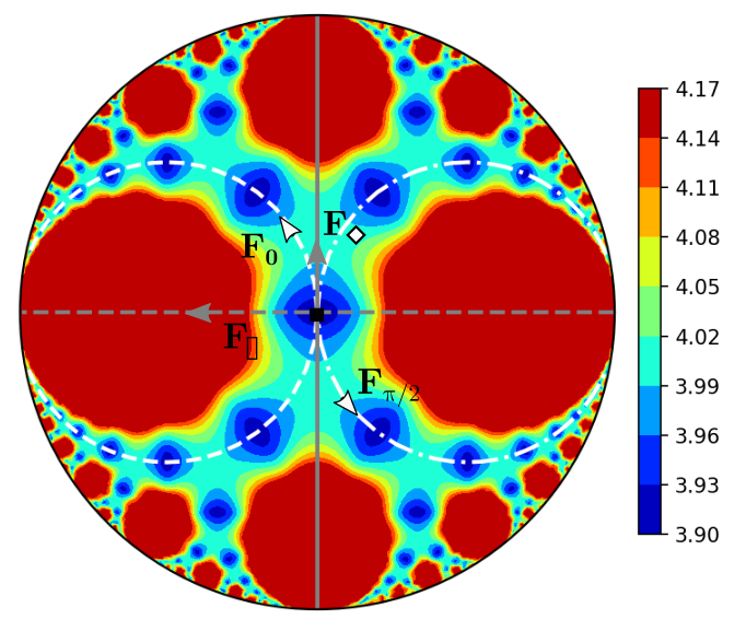
(a)

(b)

Figure 2: (a) Poincaré disk showing the energy landscape for the case $\beta=-1/4$. Minima of the energy are located on square lattice configurations. Loading paths corresponding to simple shears are illustrated in white (dashed for ${\bf F}(\alpha,0)$ and dash-dotted for ${\bf F}(\alpha,\pi/2)$. Grey lines are the rhombic pure shear ${\bf F}_{\diamond}$ (solid) and the rectangular ${\bf F}_{\framebox{\phantom{l}}}$ (dashed). (b) Energy landscape along the loading paths ${\bf F}(\alpha,0)$ and ${\bf F}(\alpha,\pi/2)$, the equivalent configurations of the square lattice are illustrated on the insets below the corresponding energy wells. Energy landscape along the rectangular and the rhombic pure shear paths ${\bf F}_{\framebox{\phantom{l}}}$ and ${\bf F}_{\diamond}$ are also shown for comparison.

The meso-scopic finite elelment grid is formed by a network of nodes, labelled by integer valued coordinates $a=1,...,N^{2}$. We assume that each element of the network is a deformable triangle and write the displacement field in the form ${\bf u}({\bf x})={\bf u}^{a}{\mathcal{N}}^{a}(\bf x)$, where ${\mathcal{N}}^{a}(\bf x)$ are the compactly supported shape functions, ${\bf u}^{a}$ are the amplitudes of nodal displacements and summation over repeated indexes effectively extends over elements containing or bounding point $\bf x$. The mesoscopic deformation gradient is then ${\bf F}(\bf x)=\mathbb{I}+\nabla{\bf u}(\bf x)$, and the equilibrium equations can be written in the form $\partial W/\partial{\bf u}^{a}=\int_{\Omega}{\bf P}({\bf F})\nabla{\mathcal{N}}^{a}({\bf x})d{\bf x}=0.$ The hard device loading is set through the displacement ${\bf u}(\alpha)=(\bar{\bf F}(\alpha)-\mathbb{I}){\bf x}$ for all nodes $a$ on the boundary of the body $\partial\Omega$, where $\bar{\bf F}(\alpha)$ is the applied deformation gradient with amplitude $\alpha$. We also performed simulations with periodic boundary conditions ${\bf u}^{B}-{\bf u}^{A}=(\bar{\bf F}(\alpha)-\mathbb{I})({\bf x}^{B}-{\bf x}^{A})$, where $A$ and $B$ are two points periodically located on the boundary of the body $\partial\Omega$. The equilibrium problem can be solved by quasi-Newton method followed by the so called NR ‘refinement’ when the initial guess is too far from the solution for Newton–Raphson method to converge initially [18].

More specifically, to find ${\bf u}^{a}$ we first use the L-BFGS algorithm [62] which builds a positive definite linear approximation allowing one to make a quasi-Newton step lowering $W$. Such iterations continue till the increment of total energy $W$ becomes sufficiently small. The obtained approximate solution is then used as an initial guess ${\bf w}^{a}$ to solve, using LU factorization [63], the equations for the correction $\text{d}{\bf w}^{a}$ which read $K^{ab}_{ij}dw_{j}^{b}+R_{i}^{a}=0,$ where $K^{ab}_{ij}=A_{iKjL}({\bf F})\frac{\partial{\mathcal{N}}^{a}}{\partial x_{K}}\frac{\partial{\mathcal{N}}^{b}}{\partial x_{L}}$ and $R^{a}_{i}=P_{iK}({\bf F})\frac{\partial{\mathcal{N}}^{a}}{\partial x_{K}}.$ The displacement field can be updated in this way till the value of the forces acting on the nodal points are sufficiently small and then the loading parameter can be advanced again, see Appendix 1 for more details.

3 Loading paths

In Figs. 2 and 3, we illustrate the energy landscapes in the cases when either square and a triangular lattice is chosen as the ground state. While some details are specific of the polynomial form of the energy density chosen in this work (say, the size of energy barriers) most of the observed features are generic and directly related to the symmetry requirements imposed on the energy. To illustrate the periodic nature of such energy we show in the insets its evolution along selected shearing deformation paths.

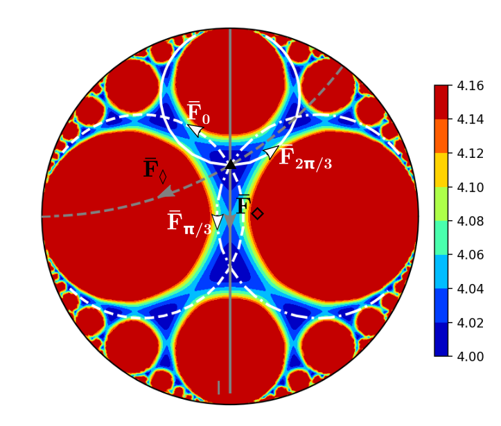
(a)

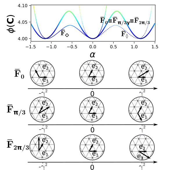
(b)

Figure 3: (a) Poincaré disk showing the energy landscape for the case $\beta=4$. Minima of the energy are located on triangular lattice configurations and simple shears form circular trajectories (shown in white). The loading paths ${\bf F}_{\diamond}$ and $\bar{\bf F}_{\lozenge}$ are illustrated in grey (with a continuous and a dashed line respectively). (b) Energy landscape along shearing deformation paths $\bar{\bf F}(\alpha,0)$, $\bar{\bf F}(\alpha,\pi/3)$ and $\bar{\bf F}(\alpha,2\pi/3)$, the shear-invariant triangular configurations are illustrated below the corresponding energy wells. The non-symmetric energy landscapes along the two pure shear paths are shown as well for comparison.

Square lattice.

Consider first the case of a lattice with square symmetry. Slip systems correspond in this case to the simple shear trajectories described by deformation gradients of the type

$$\mathbf{F}(\alpha,\theta)=\mathbf{I}+\alpha\mathbf{R}(\theta)\mathbf{e}^{0}_{1}\otimes\mathbf{R}(\theta)\mathbf{e}^{0}_{2},$$ (2)

where $\mathbf{e}^{0}_{i}$ are the vectors of the reference orthonormal basis, $\mathbf{R}(\theta)$ is an orthogonal matrix representing a clockwise rotation at the angle $\theta$ with respect to $\mathbf{e}^{0}_{1}$ and $\alpha$ is the shear amplitude parameter. The associated strain tensors ${\bf C}$ follow circular trajectories on the Poincaré disk. In Fig. 2 the white continuous and dotted circles correspond respectively to shears ${\bf F}(\alpha,\theta=0)$ and ${\bf F}(\alpha,\theta=\pi/2)$, which are oriented along close packed directions. In Fig. 2(b), we illustrate the energy landscape along such simple shear trajectories with the corresponding deformed lattice configurations shown below.

While both ’soft’ and ’hard’ simple shear loading paths were considered in detail in [18], in this paper we focus on the pure shear paths, that is, on volume preserving deformations that shrink the elementary cell of the crystal along one axis while elongating it along another one which is oriented in the perpendicular direction. We consider two pure shear loading paths for which the corresponding metric tensors $\bf C$ are non-generic as they are located on the boundaries of the fundamental domain $\bf D$. In the purely elastic regime such loading protocols transform the original square configurations into either rectangular and rhombic loaded configurations without changing their specific volumes; in what follows we use the notation $\mathbf{F}_{\diamond}$ for the rhombic pure shear and $\mathbf{F}_{\framebox{\phantom{l}}}$ for the rectangular pure shear.

Along the rhombic path the direction $-(\sqrt{2}/2){\bf e}_{1}+(\sqrt{2}/2){\bf e}_{2}$ is shortened while the direction $(\sqrt{2}/2){\bf e}_{1}+(\sqrt{2}/2){\bf e}_{2}$ is elongated with the volume of the element remaining constant. Then, ${\bf C}_{\diamond}={\bf F}_{\diamond}^{T}{\bf F}_{\diamond}={\bf U}_{\diamond}^{T}{\bf R}^{T}{\bf R}{\bf U}_{\diamond}={\bf U}_{\diamond}^{2}$, where

$${\bf U}_{\diamond} =\bm{\Psi}\bm{\Lambda}^{1/2}\bm{\Psi}^{T}=\left[\begin{array}[]{cc}\frac{\sqrt{2}}{2}&\frac{\sqrt{2}}{2}\\ \frac{-\sqrt{2}}{2}&\frac{\sqrt{2}}{2}\end{array}\right]\left[\begin{array}[]{cc}\frac{1}{\lambda}&0\\ 0&\lambda\end{array}\right]\left[\begin{array}[]{cc}\frac{\sqrt{2}}{2}&-\frac{\sqrt{2}}{2}\\ \frac{\sqrt{2}}{2}&\frac{\sqrt{2}}{2}\end{array}\right]$$ (9)

is the the stretch tensor, $\bm{\Psi}$ is the orthogonal matrix whose columns are the principal directions and $\bm{\Lambda}$ is the diagonal matrix with the squares principal stretches $\lambda_{i}$ as eigenvalues [64]. The corresponding deformation gradient, chosen in such a way that the lower side of the element is aligned with the horizontal direction during the deformation process, can be written as $\mathbf{F}_{\diamond}=\mathbf{R}_{\diamond}\mathbf{U}_{\diamond}$, where

$$\mathbf{F}_{\diamond}=\frac{1}{\sqrt{\cosh\alpha}}\left[\begin{array}[]{cc}\cosh\alpha&\sinh\alpha\\ 0&1\end{array}\right]\,,\,\mathbf{R}_{\diamond}=\frac{1}{\sqrt{\cosh\alpha}}\left[\begin{array}[]{cc}\cosh(\alpha/2)&\sinh(\alpha/2)\\ -\sinh(\alpha/2)&\cosh(\alpha/2)\end{array}\right]\,,$$ (10)

and $\alpha=\ln{\lambda}$. We note that the rhombic path is tangent to the simple shear path $F(\alpha,0)={\bf I}+\alpha{\bf e}_{1}^{0}\otimes{\bf e}^{0}_{2}$, these two deformation directions are interchangeable in the classical linear elasticity (but not in MTM).

Along the rectangular path $\mathbf{F}_{\framebox{\phantom{l}}}$ the principal directions are the reference vectors $\mathbf{e}^{0}_{1}$ and $\mathbf{e}^{0}_{2}$, therefore:

$$\mathbf{F}_{\framebox{\phantom{l}}}={\bf U}_{\framebox{\phantom{l}}}=\left[\begin{array}[]{cc}\frac{1}{\lambda}\,\,0\\ 0\,\,\lambda\end{array}\right]=\left[\begin{array}[]{cc}\cosh(\frac{\alpha}{2})-\sinh(\frac{\alpha}{2})\,\,\,\,\,\,\,\,\,\,\,\,\,\,\,\,0\\ 0\,\,\,\,\,\,\,\,\,\,\,\,\,\,\,\,\cosh(\frac{\alpha}{2})+\sinh(\frac{\alpha}{2})\end{array}\right]\,.$$ (11)

The individual elements are then elongated along the horizontal direction $\mathbf{e}^{0}_{2}$ and shortened along the vertical direction $\mathbf{e}^{0}_{1}$.

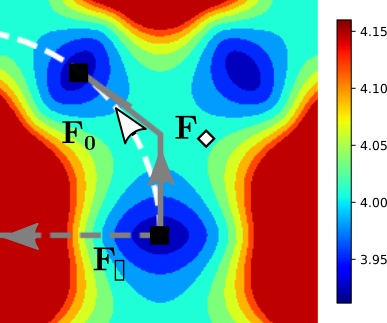
(a)

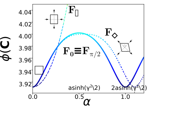
(b)

Figure 4: (a) Loading paths $\mathbf{F}_{0}$ (dashed white) , ${\bf F}_{\framebox{\phantom{l}}}$ (dashed grey) and ${\bf F}_{\diamond}$ (grey). The latter two correspond to the boundary of the periodicity domain $D$ and describe the deformations of the square lattice towards rectangular and rhombic configurations, respectively. (b) Energy landscape along the illustrated paths. The low energy path ${\bf F}_{\diamond}$ spans the bottom of the energy barrier and crosses the high symmetry point $\bf T$.

In Fig. 4(a), we the rhombic and the rectangular pure shear loading paths superimposed on the energy surface of a square crystal. One can see that the rhombic path is located inside the energy valley and can be then considered as ’soft’. Instead, the rectangular path goes against a steep energy hill and is therefore ’hard’. The corresponding one-dimensional energy landscapes are illustrated in Fig. 2(b).

Triangular lattice.

We now consider as the reference state, where the loading path begins, the triangular lattice $\bf T$. Its generating basis is given by the two vectors ${\bf e}^{\triangle}_{1}=\gamma\left\{1,0\right\}^{T}$ and ${\bf e}^{\triangle}_{2}=\gamma\left\{1/2,\sqrt{3}/2\right\}^{T}$, with $\gamma=\sqrt[4]{4/3}$. The shear paths are now characterized by the families of deformation gradients

$$\bar{\bf F}(\alpha,\theta)=\mathbf{F}(\alpha,\theta){\bf H},$$ (12)

where ${\bf H}$ is the matrix whose columns are the basis vectors ${\bf e}^{\triangle}_{i}$, ${\bf F}(\alpha,\theta)$ is shear deformation defined in Eq. 2 for simple shears (we recover closed-pack directions for $\theta=0,\pi/3,2\pi/3$). Note that with this parametrization, the value of the parameter $\alpha$ for which the lattice invariant shears for triangular symmetry are recovered is not an integer, but instead $\alpha=n\gamma^{2}$ where $n$ is integer. The energy profile along these paths $\bar{\bf F}(\alpha,\theta)$ is shown in Fig. 3(b), see [18] for more details.

Here we focus instead on pure shear loading paths originating in triangular reference state $\bf T$ and corresponding to the boundaries of the minimal periodicity domain $\bf D$. Along one of these paths, $\bar{\bf F}_{\diamond}$, we obtain lattices with rhombic symmetry where both diagonals of the rhombus are longer than the side; the other path, $\bar{\bf F}_{\lozenge}$, corresponds to the case of rhombi with one of the diagonals smaller than the side [46]. We remark that the path $\bar{\bf F}_{\diamond}$ originating in $\bf T$ describes the same deformation as the path ${\bf F}_{\diamond}$ originating in $\bf S$. In the case of triangular lattice, the principal directions are rotated by $\pi/6$ with respect to the reference axes of the square lattice, therefore, in analogy with (9) one can write

$$\bar{\bf U}_{\diamond}=\bar{\bm{\Psi}}\bm{\Lambda}^{1/2}\bar{\bm{\Psi}}^{T}=\left[\begin{array}[]{cc}\cosh(\frac{\alpha}{2})-\frac{1}{2}\sinh(\frac{\alpha}{2})&-\frac{\sqrt{3}}{2}\sinh(\frac{\alpha}{2})\\ -\frac{\sqrt{3}}{2}\sinh(\frac{\alpha}{2})&\cosh(\frac{\alpha}{2})+\frac{1}{2}\sinh(\frac{\alpha}{2})\\ \end{array}\right].$$

Among all such deformations the one which preserves the angle between ${\bf e}^{\triangle}_{1}$ and the horizontal direction is $\bar{\mathbf{F}}_{\diamond}={\bf R}(\chi)\bar{\bf U}_{\diamond}$, with: $\chi=\arctan\left(\frac{\sqrt{3}}{2}\frac{\tanh{\alpha/2}+2}{2\tanh{\alpha/2}}\right)^{-1}.$ This deformation is then applied to the triangular basis ${\bf e}^{\triangle}_{i}$. Note that along the loading path ${\bf F}_{\diamond}$, the crystal is driven trough a very shallow energy valley extending from the (triangular) energy minimum $\bf T$ towards the mountain pass represented by the (square) saddle $\bf S$ and then further to another energy (square) minimum at $\alpha=2\operatorname{arcsinh}(\gamma^{2}/2)$ (see Fig. 5). We remark that, along the ’soft’ pure shear path $\bar{\bf F}_{\diamond}$, the energy barrier, which has its maximum at $\mathbf{S}$ (with $\alpha=\text{arccosh}(\gamma^{2})$), is lower than the one along the simple shear path ${\bf F}_{\pi/3}$, the one which is habitually selected as the natural ’plastic mechanism’.

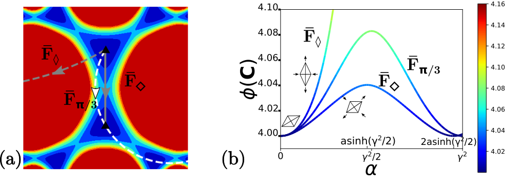
Figure 5: (a) Loading path $\bar{\bf F}_{\pi/3}$ (dashed white), $\bar{\bf F}_{\lozenge}$ (dashed grey) and $\bar{\bf F}_{\diamond}$ (grey). The latter two correspond to the boundary of $D$ and describe the deformation of the triangular lattice towards different rhombic configurations. (b) Energy landscape along the illustrated paths. The low energy path $\bar{\bf F}_{\diamond}$ spans the bottom of the energy barrier and crosses the high symmetry point $\bf S$.

The second rhombic loading path $\bar{\bf F}_{\lozenge}$ is obtained by applying the pure shear deformation ${\bf F}_{\framebox{\phantom{l}}}$ to the lattice defined by the basis vectors ${\bf e}^{\triangle}_{i}$. Along the path $\bar{\bf F}_{\lozenge}$ which is much ’harder’ than the path ${\bf F}_{\diamond}$, the energy grows very rapidly without ever passing through any other minimum, see Figure 5 .

Stability limits.

With each loading path we can associate an effective stability (yield) limit obtained under the assumption that the state is homogeneous and the discretization length scale is vanishingly small. In other words, we imply here an instability of a perfect crystal deformed in a hard device with the affine deformation $\bar{\bf F}(\alpha)$ applied on the boundary and search for the critical value of the loading parameter $\alpha_{c}$ at which the homogeneous state ceases to be stable. To identify the bifurcation point we need to solve an incremental problem defined by the tangential elastic moduli $\mathcal{A}_{iKjL}=\frac{\partial^{2}\phi}{\partial F_{iK}\partial F_{jL}}$ It is known that the homogeneous configuration remains incrementally stable in the above sense as long as the Legandre-Hadamard (strong ellipticity condition) $Q_{ij}(\mathbf{N})l_{i}l_{j}>0$ holds [65], where we introduced the acoustic tensor $Q_{ij}(\mathbf{N})=\mathcal{A}_{iKjL}N_{K}N_{L}$ while $\mathbf{N}$ and $\mathbf{l}$ are arbitrary vectors, in the reference and deformed configurations, respectively. The corresponding critical value of the loading parameter is usually found from the condition $\det Q(\mathbf{N})=0$, e.g. [66]. In what follows we use an Eulerian version of this bifurcation condition $\det\mathbf{q}(\mathbf{n})=0$, where $q_{ik}=\mathbf{a}_{ijkl}n_{j}n_{l}$, $\mathbf{a}_{ijkl}=\mathcal{A}_{iKjL}F_{kK}F_{lL}$ and $\mathbf{n}=\mathbf{F}^{-T}\mathbf{N}$. The Eulerian vectors $\bf n$ and $\bf l$ characterize the incipient unstability mode [67]. For instance, if $\bf n$ is approximately perpendicular to $\bf l$. In the post-bifurcational regime one can expect in this case the formation of (lattice size) shear bands along the plane with normal $\bf n$ and with slip direction $\bf l$ [28]. Further development may lead to the nucleation inside the individual bands of incipient dislocation pairs (slip embryos in 2D or dislocation loops in 3D) whose Burgers vector is aligned with $\bf l$ or to the collective process resulting in activation of a micro-twin laminate with the twinning plane oriented along $\bf n$.

(a)

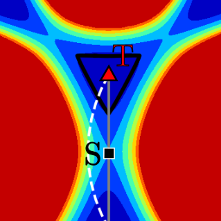
(b)

Figure 6: (a) Stability (yielding) limits for the square crystal (in black). The two loading paths corresponding to simple shear ${\bf F}_{0}$ (dashed white) and rhombic pure shear ${\bf F}_{\diamond}$ (grey) cross the stability region in similar configurations. (b) Stability region for the triangular symmetry crystal (black). Here the difference of strain configurations at the limit of stability is larger if we compare the loading paths corresponding to simple shear (dashed white) and pure shear (grey).

Using the proposed approximate stability condition we can delineate in the configurational space of metric tensors $\bf C$ a region around the reference state where the continuous homogeneous system can be expected to be stable and interpret it as an effective ’yield surface’. To this end we need to consider a sufficiently broad family of loading paths, for instance, the family of simple shear trajectories with the full range of values of the shearing angle $\theta$ plus the two limiting loading paths along the boundary of the periodicity domain $\bf D$ and representing pure shears (the paths ${\bf F}_{\framebox{\phantom{l}}}$ and ${\bf F}_{\diamond}$ for the square lattice, and $\bar{\bf F}_{\diamond}$ and $\bar{\bf F}_{\lozenge}$ for the triangular lattice). Along each of these paths we computed the first value of the loading parameter $\alpha$ where the Legandre-Hadamard condition is violated for some non-trivial $\bf n$ and $\bf l$. This produced an effective ’yield surface’ which we illustrated by black lines in our Figures 6(a) and 6(b) for square and triangular lattices, respectively.

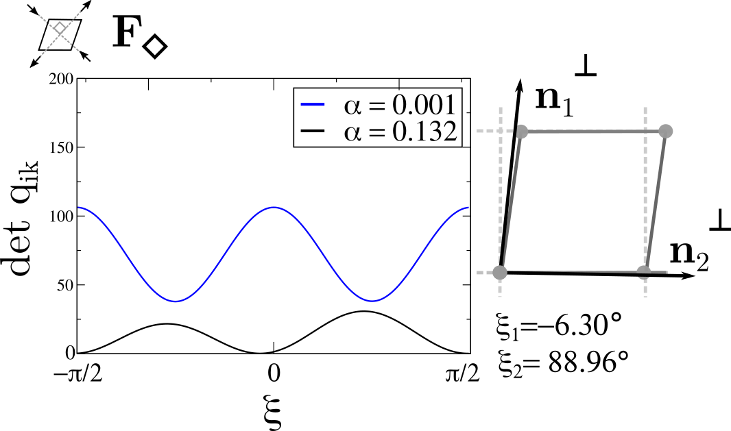
(a)

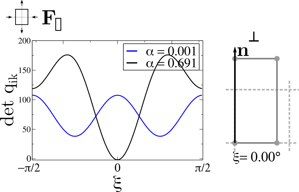
(b)

Figure 7: The function $\det\left({\bf F}(\alpha),{\bf n}(\xi)\right)$ is illustrated for $\alpha=0.001$ and $\alpha=\alpha_{c}$ for the two deformation paths considered in the case of the square crystal, that is ${\bf F}_{\diamond}$ (a) and ${{\bf F}}_{\framebox{\phantom{l}}}$ (b).

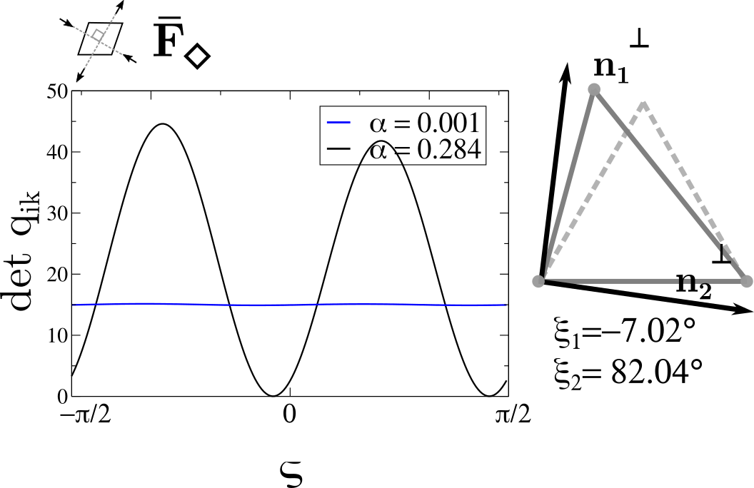
(a)

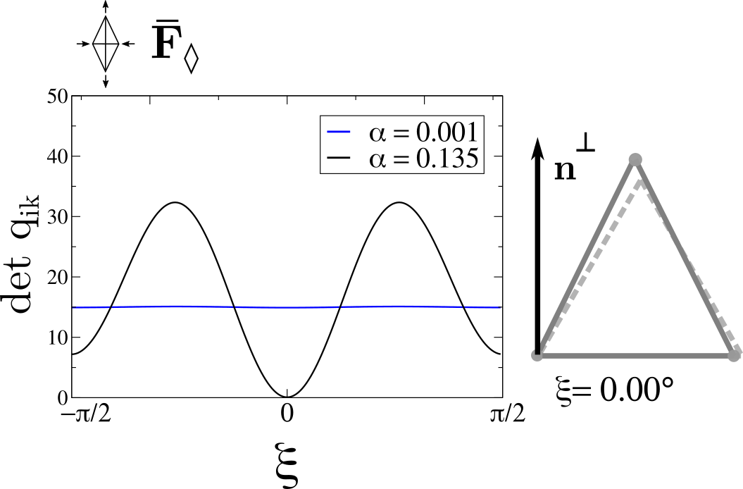
(b)

Figure 8: The function $\det\left({\bf F}(\alpha),{\bf n}(\xi)\right)$ is illustrated for $\alpha=0.001$ and $\alpha=\alpha_{c}$ for two deformation paths considered in the case of the triangular crystal, that is $\bar{\bf F}_{\diamond}$ (a) and ${\bar{\bf F}}_{\lozenge}$ (b).

We illustrate the nature of the instability modes for square and triangular lattices loaded along the special pure shear paths. If the potentially unstable orientation $\bf n$ is parametrized by the angle $\xi$ as $\bf n=\left\{\cos\xi,\sin\xi\right\}$ it is of interest to study the $\xi$ dependence of the parameter $\det\mathbf{q}(\mathbf{n})$ at different values of $\alpha$ and in our Fig. 7 and Fig. 8, we show such graphs for $\alpha=0$ and $\alpha_{c}$ for all four pure shear loading paths discussed above. In the inset located to the right of each of these plots we represented the directions ${\bf n}^{\perp}$ indicating the orientation of the unstable (slip) plane vis a vis the basis vectors of the deformed crystal at the onset of instability ( along with the values of $\xi$). We note that for the rectangular path ${\bf F}_{{\framebox{\phantom{l}}}}$ for the square and $\bar{\bf F}_{\lozenge}$ for the triangular lattices the unstable mode is perfectly aligned with the horizontal plane (${\bf n}^{\perp}$ is aligned with the vertical directions). The polarization vectors $\bf l$ were found to be approximately perpendicular to $\bf n$ for all of the investigated loading directions.

We remark that the simple shear type loading paths were discussed in detail in [18] where we showed that for square lattices the instability along the (’soft’) simple shear direction ${F}_{\theta=0,\alpha}$ produces two almost simultaneous instability modes with the resulting activation of two crystallographic slip systems. We have seen that such modes are also almost simultaneous in the case of square lattices subjected to the (’soft’) pure shear loading ${\bf F}_{\diamond}$. Moreover, the analysis of the (’soft’) path $\bar{\bf F}_{\diamond}$ for triangular lattices shows the analogous effect ( which is not apparent along crystallographic-oriented simple shears). Along the generic (’hard’) shearing directions (implying both pure and simple shears), there is only one unstable mode $\bf n$ which reflects the activation of a single slip system.

4 Numerical experiments

In this section we present the results of our numerical simulations. Their main goal is to provide first evidence of the efficiency of MTM in addressing various sub-continuum problems in crystal plasticity. Throughout this section we use the version of the model, the numerical algorithm and the loading protocols described in the previous sections.

Dislocation cores.

To interpret the obtained data in experiments involving large number of dislocations, it is important to be able to identify and resolve the structure of individual dislocation cores. That is why we begin with consideration of an isolated dislocation trapped by the discreteness of the meso-scopic lattice in the center of a sufficiently large unloaded crystal.

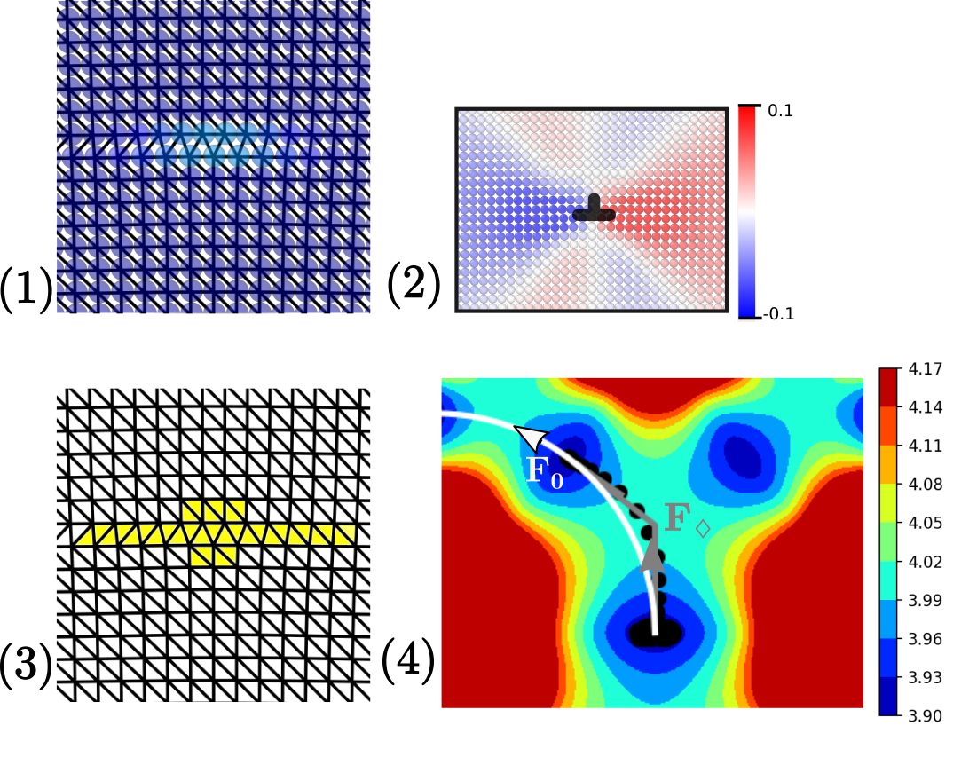
(a)

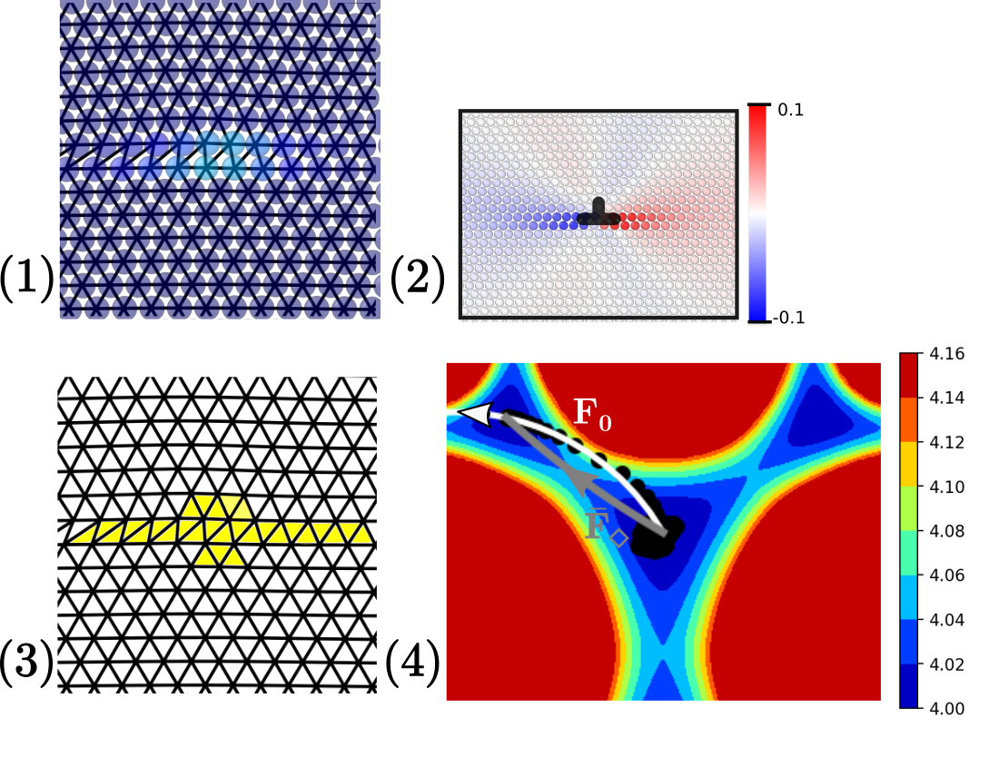
(b)

Figure 9: (a) Dislocation structure in the case of square lattice: (1) energy near the core, (2) Cauchy stress $\sigma_{xy}$, (3) a detail of the elements triangulation, (4) elements strain projection on $\bf C$ space, color bar shows the energy level both in (a) and (b). (b) Dislocation structure for the triangular symmetry crystal. Pictures are analogous to (a).

As we have already mentioned, dislocations can appear in MTM when different variants of the same lattice (different phases) are present simultaneously. Consider, for instance, the coexistence in the square lattice of the reference phase ${\bf S}={\bf F}(\theta=0,\alpha=0)$ and the phase ${\bf S}_{1}^{0}={\bf F}(\theta=0,\alpha=1)$ which is different from the reference phase by an elementary lattice invariant shear. A single dislocation is obtained in the configuration where a semi-infinite single layer of elements in phase ${\bf S}_{1}^{0}$ is embedded in an infinite lattice of elements in phase ${\bf S}$, see Fig. 9(a). Far away from the area around the terminal point of the sheared (slipped) layer of elements, which represents the dislocation core, the lattices are perfectly compatible because all such elements lie in the bottoms of the corresponding energy wells. Elements in the core region lie outside the energy wells and have therefore nonzero elastic energy.

To obtain in a numerical experiment an isolated dislocation we used a square domain (with $200\times 200$ finite element nodes) and applied on its boundary the displacement field reproducing anticipated far field continuum asymptotics (Volterra dislocation, [68]), $u_{x}=\frac{b}{2\pi}\left[\arctan\frac{y}{x}+\frac{xy}{2(1-\nu)(x^{2}+y^{2})}\right]$ and $u_{y}=\frac{b}{2\pi}\left[\frac{1-2\nu}{4(1-\nu)}\ln(x^{2}+y^{2})+\frac{x^{2}-y^{2}}{4(1-\nu)(x^{2}+y^{2})}\right]$. The configuration of the nodes was then allowed to relax elastically till the local minimum of the energy was reached. As a result of such relaxation an isolated dislocation core was formed in the middle of the domain whose different representations (energy, stress, deformation) are shown in Fig. 9(a) for the case of square lattice and in Fig. 9(b) for the case of triangular lattice. In Figs. 9 (a-4,b-4) we show the corresponding core structures in the configurational space of metric tensor.

From the deformed configuration of the elastic elements shown in Fig. 9(a-3), one can see the sheared layer to the left of the (square) dislocation core representing the (square) energy well ${\bf S}_{1}^{0}$ while the elements in the same layer but located on the right side of the dislocation core are in reference (square) well ${\bf S}$. Similarly, we see in Fig. 9(b-3) that the (triangular) dislocation core can be viewed as a domain boundary separating the coexisting elements of the two neighboring (triangular) energy wells ${\bf T}^{1}_{0}$ and $\bf T$. The presence of all these energy wells becomes even more clear as one looks at the values of the components of the metric tensors $C_{11},C_{12},C_{22}$ at the elastic elements which allows one to represent the structure of a core as a (in reality, somewhat blurred) trajectory in the configuration space, see our Fig. 9(a-4) and Fig. 9(b-4). While the initial and the final points in such trajectories are located at the bottoms of the corresponding energy wells, the trajectories themselves represent a mountain pass type connections between the wells. In the case of square crystals such trajectory ensures that the maximal elevation is minimal but apparently, this is not the case for triangular crystals. This confirms that while for both square and triangular lattices most of the transitions takes place close to the bottoms of the energy valleys, the fine structure of the barriers is manifestly symmetry dependent.

Thus, in the case of the square lattice, the trajectory describing a dislocation core appear to consist of two separate segments (shown in grey in Fig. 9(a-4) representing pure shears of the type ${\bf F}_{\diamond}$ studied in the previous section. Each of them connects the corresponding square wells (the reference well $\mathbf{S}$ and the equivalent well $\mathbf{S}^{-1}_{\pi/2}=\mathbf{F}_{\pi/2}(\alpha=-1)$ reachable by an elementary lattice invariant shear) with the shallow local minimum (almost a monkey saddle for our choice of the potential, see [37]) describing the triangular (hexagonal) lattice $\bf T$. Here the configuration $\bf T$, whose presence in the core structure is also suggested also by the configuration of the elements shown in Figure 9 (1c), plays here the role of a stacking fault while the pure shears can be interpreted as the analogs of Shockley partials, see for instance [69, 70, 71]. Note that the naively favored simple shear trajectory ${\bf F}_{0}$ (shown in white in Figure 9 (1-d)) delivers, as we have seen before, a slightly higher barrier and is therefore avoided by the solution of the energy minimization problem.

The structure of the dislocation core in triangular lattices is different. Thus, the corresponding mountain pass type trajectory in the configurational space (shown in white in Fig. 9(b-4)) follows the simple shear path ${\bf\bar{F}}_{0}$. An alternative trajectory consisting of two pure shear segments and passing through the square energy configuration ${\bf S}$ (shown in gray in Fig. 9(b-4)) is not taken by the system despite being characterized by a lower energy barrier (see Fig. 5).

Collective nucleation of dislocations.

Now, instead of the specially designed non-affine boundary conditions ensuring the emergence of a single dislocation, we consider generic affine loading paths and study the symmetry breaking decomposition of the homogeneous state. More specifically, we assume that the system is driven quasi-statically and therefore evolves through a sequence of equilibrium configurations. In the absence of pre-existing defects (pristine crystal), the initial evolution of the system from the unloaded reference state is elastic till the corresponding elastic branch of equilibria ceases to exist. At the point of instability the dissipative branch-switching event, accompanied by a macroscopic stress, drop takes place. It takes the form of a system size avalanche leading to collective nucleation of a large number of dislocation and a global slip-induced reorganization of the crystal lattice.

Consider, for instance, the case of a square domain $\Omega$ with $N=100\times 100$ nodes and assume that the applied affine deformation is a homogeneous simple shear $\bar{\bf F}(\alpha,\phi)$ with fixed orientation $\phi$, and the shear amplitude $\alpha$ playing the role of the loading parameter. By changing this parameter in increments of $10^{-4}$, we can advance the displacement field ${\bf u}(\alpha,\phi)=(\bar{\bf F}(\alpha,\phi)-\mathbb{I}){\bf x}$ for all nodes on the boundary of the body $\partial\Omega$ till the first instability occurs signaling the homogeneous dislocation nucleation. The incremental solution algorithm allowing one to see the unfolding of the avalanche in the fast computational time is detailed in the flowchart shown in Appendix A. In [18] we showed that the resulting (post-avalanche) dislocation pattern depends on the orientation of the applied simple shear with a strong difference between the dislocational configurations obtained in the cases of soft and hard loading directions. In the present paper, we illustrate results obtained along the pure shear loading protocols using periodic boundary conditions where the system was loaded starting from a stable reference configuration till the point of instability close to the theoretically predicted elastic instability, see Fig. 10(a) and Fig. 10(b). Results obtained along the same loading paths but the fixed boundary conditions are comparable in terms of observed collective dislocation mechanisms, but since they tend to display a stronger influence of the boundaries we are not discussing them here in detail.

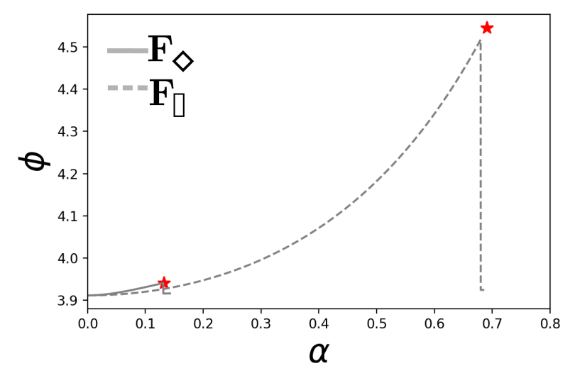
(a)

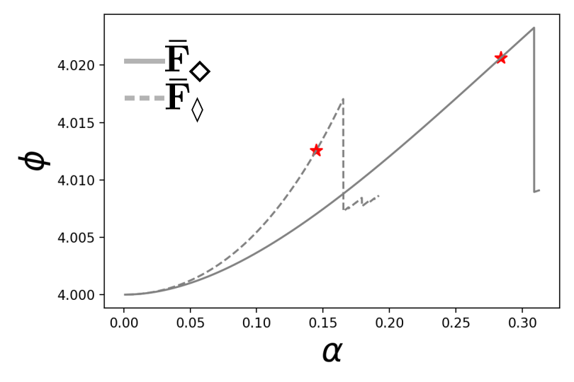
(b)

Figure 10: Energy-strain relations obtained in numerical experiments for a crystal with square symmetry: (a) and for a crystal of triangular symmetry (b). Simulated domains are formed by $N\times N$ nodes with $N=100$, loaded with affine boundary conditions. Red stars display the critical parameters calculated analytically.

Here we report the results of the numerical experiments obtained for the pure shear loading protocols discussed in the previous section. These loading paths are of particular interest since they include the ’softest’ and the ’hardest’ loading directions which correspond to the ’shortest’ and the ’longest’ distance to instability’, respectively. These loading paths are also highly symmetric which suggests that the post avalanche dislocation patterns may have some particular features. Thus, as we have already seen, among the two pure shear loading directions, one is always directed towards the energy maximum and can be expected to produce regular micro-twin microstructures. Another one is aiming directly at the mountain pass where the corresponding saddle point may foment the generation of disorder.

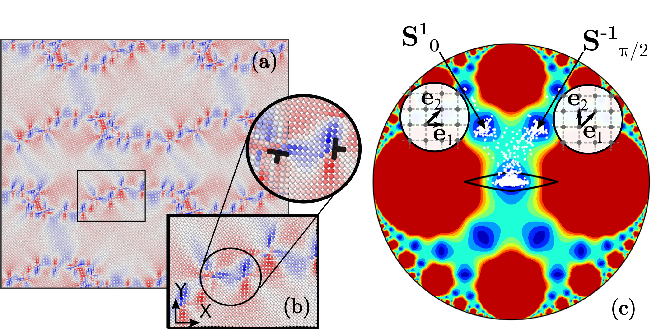
Figure 11: (a) Post-instability pattern for the rhombic path ${\bf F}_{\diamond}$, colors show the level of the Cauchy stress $\sigma_{xy}$. (b) Inset highlights the presence of both vertical and horizontal dislocations. (c) Distribution of ${\bf C}_{i}$ points in configuration space show the dominant presence of the three wells $\bf S$, ${\bf S}^{1}_{0}$ and ${\bf S}_{\pi/2}^{-1}$. The elements on the low energy valleys connecting wells corresponds to dislocation cores.

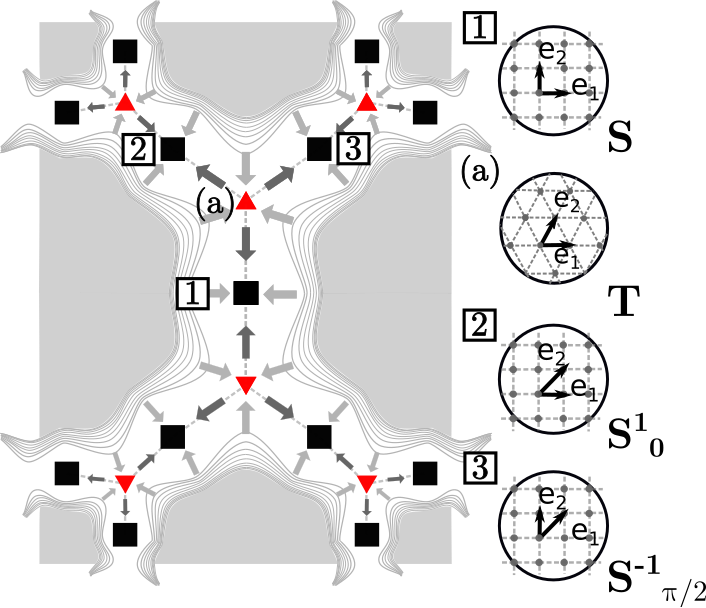
Figure 12: Schematic representation of the saddle-like structure of the triangular phases in the square symmetry crystal. When the reference square configuration (1) is loaded along the energy valley, the systems encounters the triangular phase (a) and here splits along two different slip system, thus involving two additional wells (2) and (3). This splitting mechanism presents every time a square phase is loaded towards a triangular one.

Square lattices.

We start with the case of a square lattice loaded along the ’soft’ rhombic loading path ${\bf F}_{\diamond}$. The fragment of the post-instability pattern, shown in Fig. 11(a); the colors in this image representing the physical space indicate the level of the Cauchy stress $\sigma_{xy}$. The observed simultaneous activation of both available slip systems is compatible with the emergence of two unstable modes in the linear analysis which suggests dislocation nucleation along the planes with two types of normals ${\bf n}_{i}$. We note the concurrent initiation of the horizontal and vertical slip systems has been already observed in [18] for the case of the simple shear loading path ${\bf F}_{\theta=0}$.This is not surprising since the two paths corresponding to simple and pure shear cross the stability boundary in configurations which are very close to each other in $\bf C$ space.

The obtained dislocation pattern can be understood further if we represent it in the configurational space of metric tensors, see our in Fig. 11(b). In the homogeneous elastic state all configurational points were in the same location which depended parametrically on the loading parameter $\alpha$. After the effective yield surface was reached the configurational points spread over the configurational space with most of them concentrating in the three equivalent energy wells corresponding to the reference square lattice ${\bf S}$, and the equivalent square lattices ${\bf F}_{0}(\alpha=1)$ and ${\bf F}_{\pi/2}(\alpha=-1)$ which differ from the reference lattice by lattice invariant shears along the two perpendicular slip direction. Since the corresponding states have zero energy, such a localization indicates the formation of unloaded square lattice patches (grains) which differ only by rotation. The points outside the energy wells are mostly located inside the energy valleys connecting the reference lattice ${\bf S}$ with equivalent configurations ${\bf F}_{0}(\alpha=1)$ and ${\bf F}_{\pi/2}(\alpha=-1)$, and corresponding to the horizontal and vertical dislocation core structures. Those structures are not exactly built as the pairs of pure shear partials studied above because they form grain boundaries (dislocation walls) where dislocation interaction is strong.

We remark that the discussed coupling between the slip systems is not postulated phenomenologically, as it is usually done in conventional continuum theories of crystal plasticity, but emerges directly from the postulated global symmetry of the energy landscape. We illustrate this point in our Fig. 12 where we show the zoom in on the schematic energy landscape in the configurational space around the reference energy well ${\bf S}$. This figure emphasizes the presence of the valleys which represent the classical ’plastic mechanisms’ and direct the flow of configurational points away from the energetically expensive purely elastic deformation. It shows that an exit from the narrow stability neighborhood of the point ${\bf S}$ (elastic domain) leads to the flow of the configurational points towards the degenerate saddle regions corresponding to the triangular lattice with the higher symmetry than the symmetry of the reference state; we note the triangular lattice automatically corresponds to a critical point due to the global symmetry of the energy landscape.

For instance, suppose that the system is driven along the rhombic loading path ${\bf F}_{\diamond}$. It is then forced directly towards the mountain pass around the point ${\bf T}$ where the system is confronted with a (binary) choice between moving either towards the (square) well ${\bf F}_{0}(\alpha=1)$ or the (square) well ${\bf F}_{\pi/2}(\alpha=-1)$ or, as in real numerical experiments, moving in both directions simultaneously while activating in this way both slip systems (here we are not talking about the configurational points that simply relax into the reference state). In the case of a less symmetric loading path, like for instance, the simple shear path ${\bf F}_{\theta=0}$, the choice will be slightly biased with both slip systems still available due to the superior symmetry of the saddle region. It is clear that when the system is loaded beyond the first avalanche, a succession of similar binary choice enhances the complexity in the developing pattern even further.

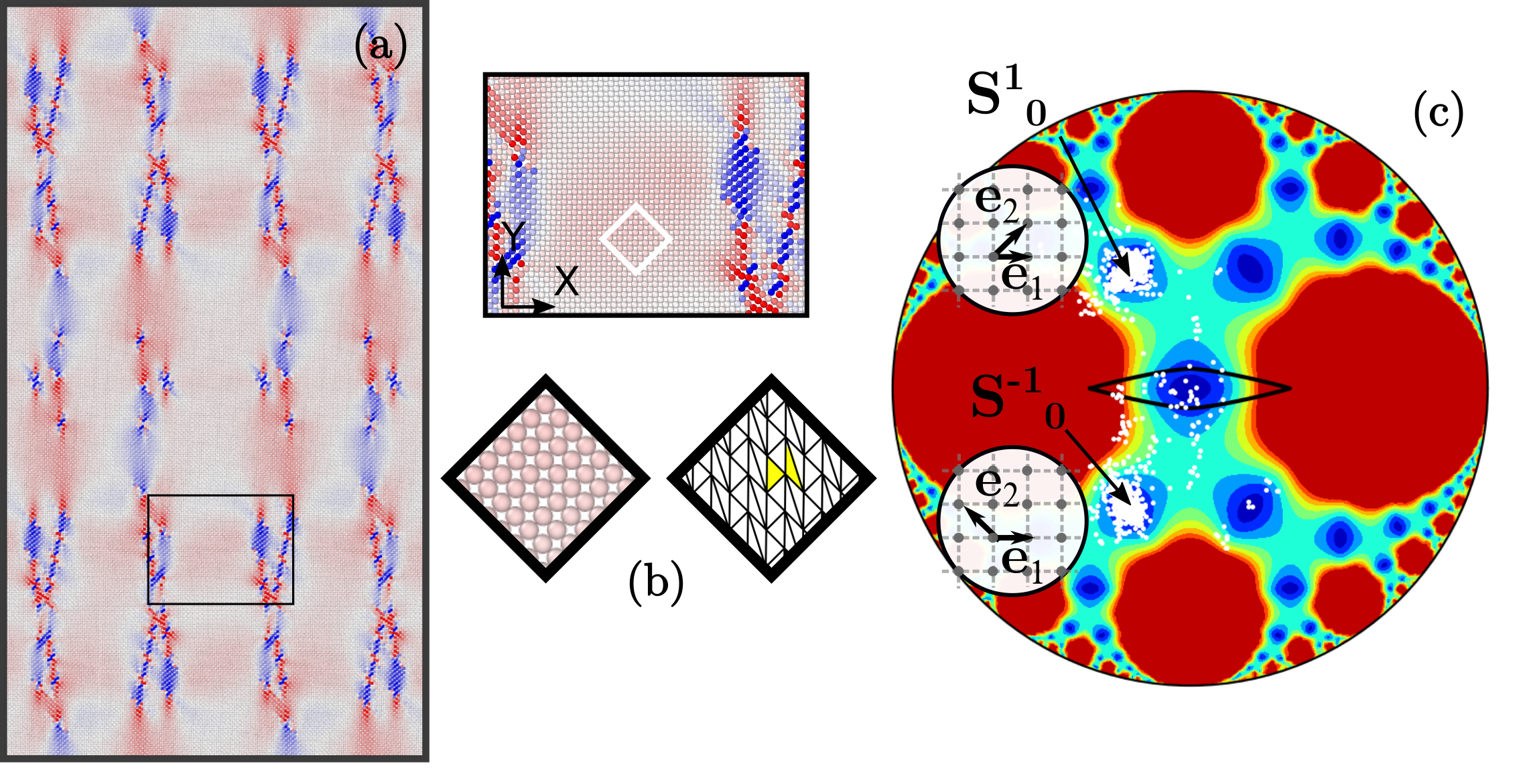
Figure 13: (a) Post-instability pattern for the rectangular path ${\bf F}_{{\framebox{\phantom{l}}}}$, colors indicate the level of the Cauchy stress $\sigma_{xy}$. (a) The insets allow one to visualize the $\pi/4$ rotated structure, the triangulation reveals the shearing mechanism behind such apparent rotation. (c) Distribution of ${\bf C}_{i}$ points in configuration space show the splitting of the system between the wells ${\bf R}^{\pi/4}{\bf S}^{1}_{0}$ and ${\bf R}^{-\pi/4}{\bf S}^{-1}_{0}$.

We now discuss the ”hard” loading path $\mathbf{F}_{\framebox{\phantom{l}}}$ corresponding to driving through the imposed on the boundary affine rectangular pure shear. We recall that in this case the square elements of the reference lattice are deformed elastically into rectangles with progressively higher energy cost. As we have also seen before, the instability of the ensuing rectangular lattice leads to the formation of the sheared layers oriented perpendicular to the long axis of the rectangles which is a horizontal direction and with their shear amplitude aligned with the vertical direction. The direction of the shear presents a binary choice between the (square) energy wells ${\bf S}_{1}^{0}={\bf F}(\theta=0,\alpha=1)$ and ${\bf S}_{-1}^{0}={\bf F}(\theta=0,\alpha=-1)$ which suggests micro-twinning mechanism of instability.

The post avalanche configuration obtained in the corresponding numerical experiment is illustrated in Fig. 13. The analysis of the physical state reveals the system size pattern where patches of the original square lattice structure appear to be rotated at $\pi/4$. The dislocation rich high energy defects serve again as the boundaries separating these grains, see Fig. 13(a). The deformed configuration of the elements inside the grains shows that the apparent rotation is produced by the fine lamination of the (almost) unloaded states from the different energy wells ${\bf S}_{1}^{0}$ and ${\bf S}_{-1}^{0}$, see Fig. 13(b). The implied two-well redistribution is clearly visible in the configurational space, shown in Fig. 13(c), where we see that these two wells are almost equally populated with almost no elements flipping back into the original energy well ${\bf S}$. This type of accommodation through inelastic rotation can be easily understood if we observe that the two sheared state configurations constituting the micro-twin laminate, ${\bf F}=\mathbf{R}(\pi/4){\bf S}^{0}_{1}$ and ${\bf G}=\mathbf{R}(-\pi/4){\bf S}^{0}_{-1}$ satisfy the compatibility condition [54] $\mathbf{F}={\bf I}+\left(\mathbf{a}\otimes\mathbf{n}\right){\bf G},$ where ${\bf a}^{T}=\left(0,2\right)$ and ${\bf n}^{T}=\left(1,0\right)$, see Fig. 14(a). Note that the normal to the twinning plane $\bf n$ coincides with the instability direction predicted by our approximate stability analysis.

In Fig. 14(b) we show the distribution of the configurational points immediately following the onset of instability, when the avalanche is only unfolding. It suggests that a highly inhomogeneous configuration precedes the development of the micro-laminates disguised as uniformly rotated grains. The eventual equilibration is achieved through the advancement of a dynamic front. Inside such a transition front the apparent rotation of the lattice is achieved through transverse motion of dislocations which nucleate inside the computational domain but ultimately annihilate on the boundary [41].

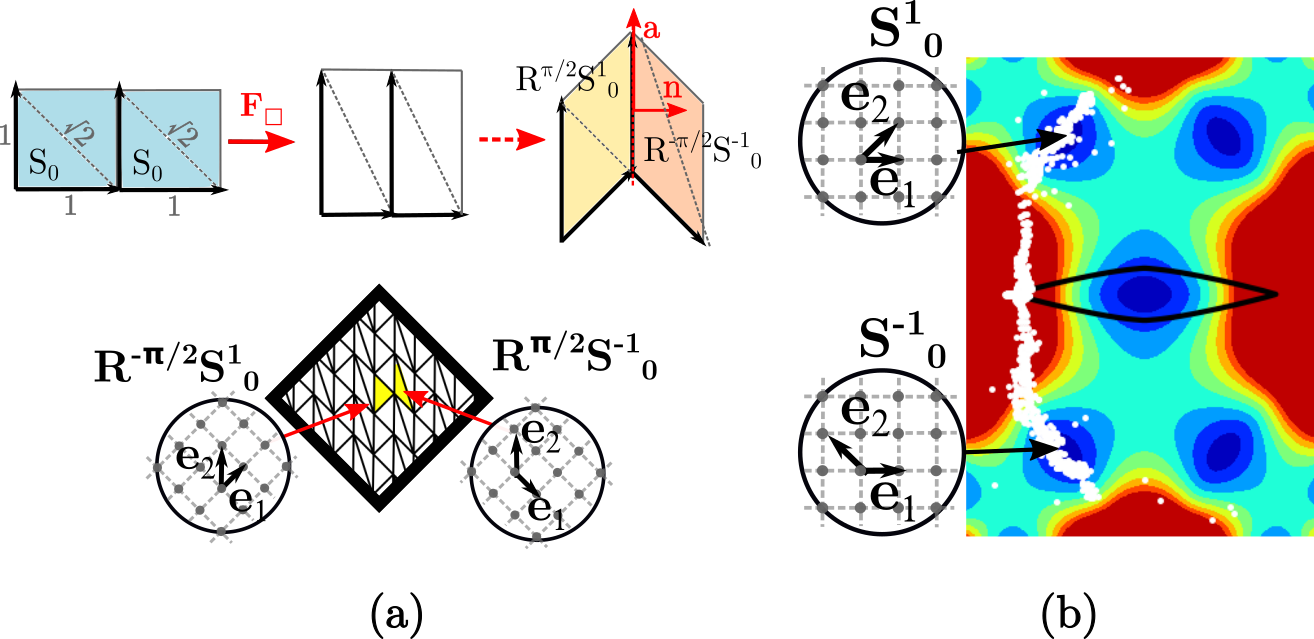
Figure 14: (a) The twinning mechanism behind the apparent rotation. The instability develops with a redistribution of the elements between the energy wells ${\bf R}^{\pi/4}{\bf S}^{1}_{0}$ and ${\bf R}^{-\pi/4}{\bf S}^{-1}_{0}$. (b) A snapshot of the developing instability, showing the early evolution of the system towards the two equivalent wells.

Triangular lattices.

Consider now the ’soft’ pure shear loading protocol $\bar{\bf F}_{\diamond}$ applied to a triangular lattice. In Fig. 15(a) we show a fragment of the post avalanche pattern in the physical space; the corresponding distribution of the configurational points is presented in Fig. 15(b). As in the case of ’hard’ pure shear loading of a square crystal, here we again see the emergence of slip on two slip systems (out of three available in general). We recall that also according to the linear stability analysis two slip directions are activated simultaneously. Interestingly, and differently from the case of square symmetry, in our numerical experiments involving triangular lattices loaded by simple shears along the closest crystallographic directions to $\bar{\bf F}_{\diamond}$, for instance $\bar{\bf F}_{\pi/3}$ or $\bar{\bf F}_{0}$, such double activation of two slip systems does not take place [18]. This is related to a structurally different organization of the low energy valleys around the reference states for square and triangular crystals and the resulting different mismatch between the critical stability thresholds along simple and pure shear loading paths.

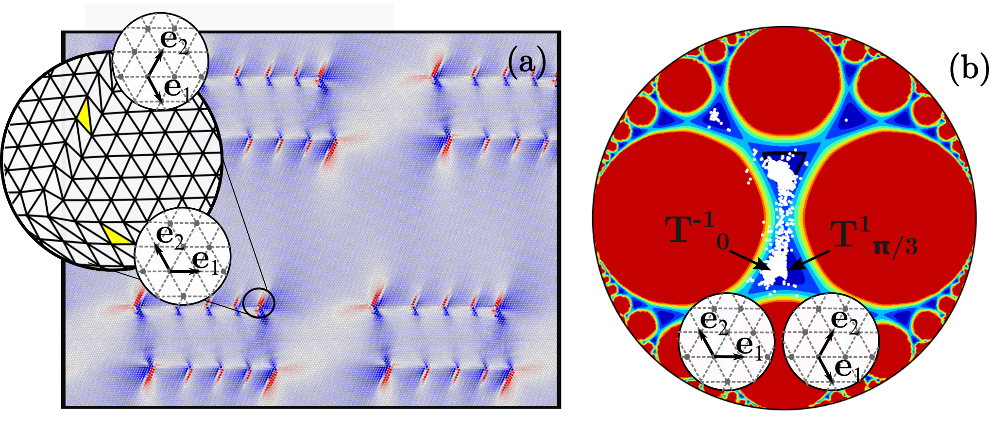
Figure 15: (a) Post-instability pattern observed on the rhombic path $\bar{\bf F}_{\diamond}$, colors indicate the level of the Cauchy stress $\sigma_{xy}$. The inset shows a detail of the triangulation revealing the activation of two slip systems. (b) Distribution of ${\bf C}_{i}$ points in configuration space show that the majority of points lies in the low energy valleys connecting $\bf T$ with ${\bf T}^{-1}_{0}$ and ${\bf T}_{\pi/3}^{-1}$. Since these two configurations differs by a rigid rotation only, the paths are overlapping.

Note first that in the case of triangular lattices, the loading paths $\bar{\bf F}_{\pi/3}$ and $\bar{\bf F}_{\diamond}$ intersect the boundary of the elastic (stability) region in the configurational points that are rather distant from the point where such crossing takes place for the pure shear path $\bar{\bf F}_{\diamond}$ while in the case of square lattices all three paths cross the stability boundary at almost the same point (compare Fig. 5 and Fig. 4). In other words, the triangular lattice, driven along the path $\bar{\bf F}_{\diamond}$, becomes unstable in the middle of the energy valley, quite late vis a vis the instability under the simple shear protocols $\bar{\bf F}_{0}$ and $\bar{\bf F}_{\pi/3}$. The fact that this happens close to the saddle S facilitates the coupling between the slip systems oriented at the angles $\theta=\pi/3$ and $\theta=0$.

Note next that while the simple shear loading paths $\bar{\bf F}_{\pi/3}(\alpha)$ and $\bar{\bf F}_{0}(-\alpha)$ are distinct, they intersect not only at $\alpha=0$ (at the reference energy well ${\bf T}$) but also at $\alpha=\gamma^{2}$ ( at the equivalent energy well ${\bf T}^{-1}_{2\pi/3}$, where the pure shear loading path $\bar{\bf F}_{\diamond}$ ultimately leads. The fact that the two simple shear paths are ultimately getting closer to the main driving direction contributes to the ultimate activation of both slip systems.

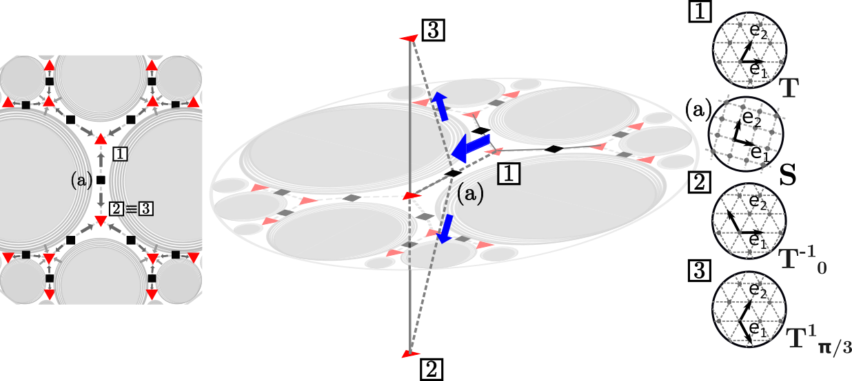
(a)

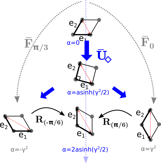
(b)

Figure 16: (a) Schematic representation of the saddle-like structure of the square phases in the triangular symmetry crystal. An extra dimension (here showed with vertical lines) needs to be included to observe rotated wells along the same orbit, that in these case intervene when considering the shears aligned with the crystallographic planes (oriented). Here we consider the reference triangular phase (1), loaded towards the square phase (a). The system ends up activating two slip system whose corresponding wells are distinguished by a rigid rotation. (b) Pure shear (Eq. 3) and simple shears $\bar{\bf F}_{\pi/3}(\alpha=\gamma^{2})$, $\bar{\bf F}_{0}(\alpha=-\gamma^{2})$ leads to formation of different patterns comprised of energy wells distinguished solely by a rigid rotation; (c) The symmetric rotations disguising two simple shears as one pure shear

We remark that, while activation of the two slip systems is clearly visible in physical space, see Fig. 15(a), it is less apparent from the spreading of the cloud of configurational points in the space of metric tensors, see Fig. 15(b) where we see that at the saddle ${\bf S}$ about half of the elements flip back to the original well ${\bf S}$ while another half advances to the new well ${\bf T}^{-1}_{2\pi/3}$. However, the two states $\bar{\bf F}_{\pi/3}(\alpha=\gamma^{2})$ and $\bar{\bf F}_{0}(\alpha=-\gamma^{2})$, which occupy the same point ${\bf T}^{-1}_{2\pi/3}$ in our conventional configurational space of metric tensors, differ by a rigid rotation.

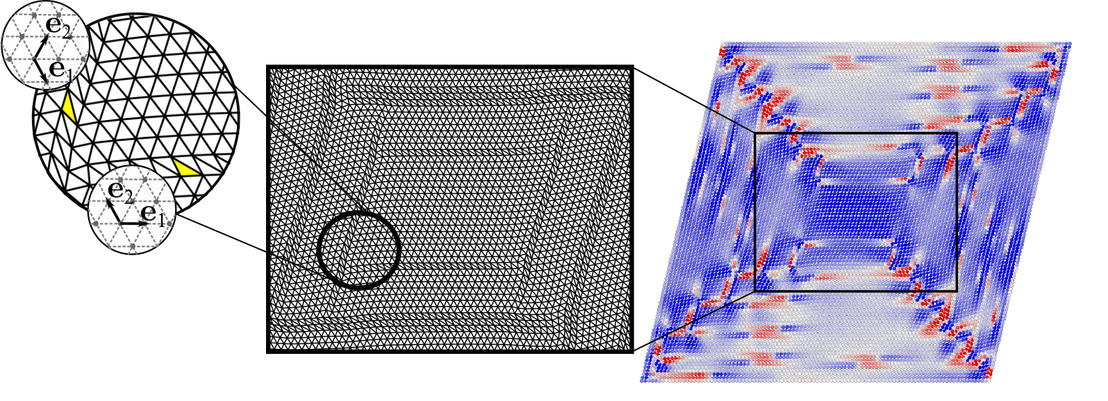
Figure 17: Post-instability pattern for the rhombic path $\bar{\bf F}_{\diamond}$, observed with fixed boundary conditions.

To explain this point we recall that even though the two configurations may belong to the same energy well, they may correspond to different points of the orbit of this well and formed by rotations which leave the metric tensor unchanged [54]. In Fig. 16 we illustrate by a scheme, a likely mechanism of the simultaneous activation of the two slip systems. While the horizontal plane in this scheme represents our conventional configurational space of metric tensors (see also the inset to the left of the scheme), the vertical direction mimics a one-parameter space of rigid rotations which we neglected in all previous considerations. When the triangular lattice ${\bf T}$, marked as (1), evolving along the energy valley, reaches the saddle describing the square lattice ${\bf S}$, marked as (a), two rotations of the same amplitude but of different signs start to develop as the system continues to evolve along the energy valley down from the saddle ${\bf S}$ towards the energy well ${\bf T}^{-1}_{2\pi/3}$, while fully maturing as symmetric slips along the close packed directions $\theta=\pi/3$ and $\theta=0$.

In Fig. 17 we show, for comparison, the post-avalanche pattern in the same setting but with fixed affine boundary conditions. While it has the same elementary local dislocational patterns as in the case of the periodic boundary conditions, the global organization is largely shaped by the influence of the boundaries. This and other finite size effects will be considered in more detail in a separate publication.

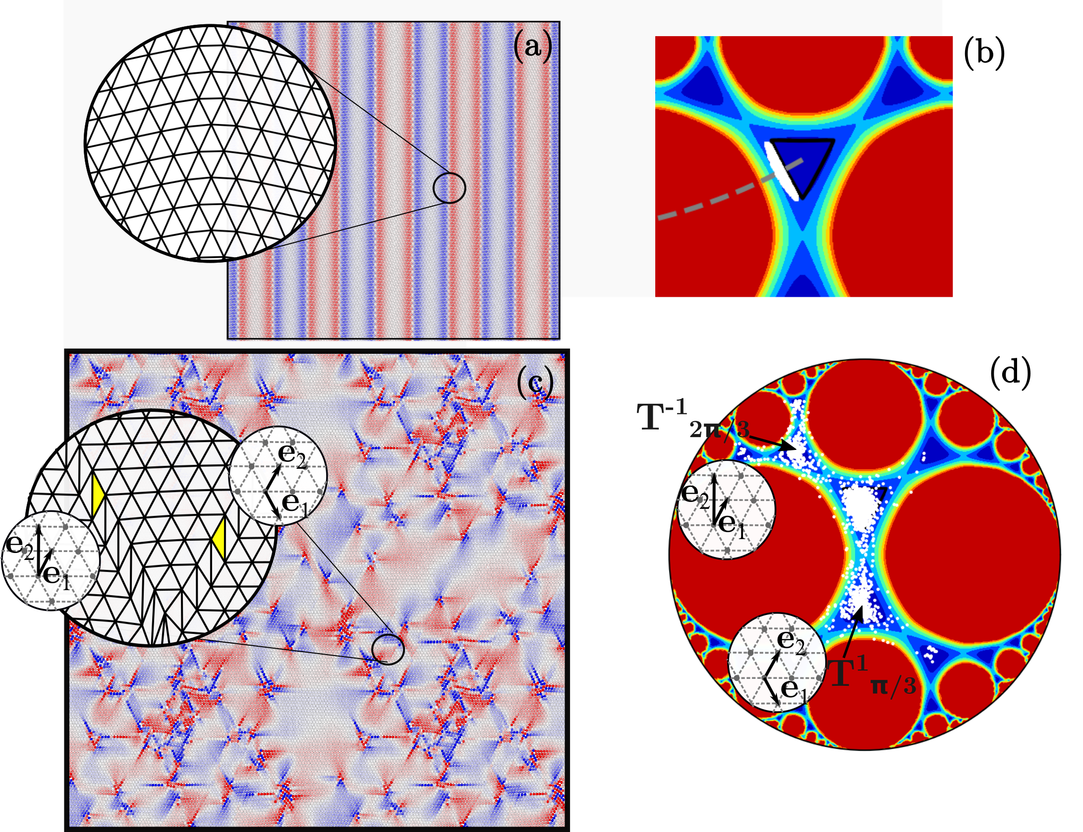
Figure 18: (a) The emerging inhomogeneous configuration at the point of instability, characterized by a pattern of weakly rotated triangular lattices; the corresponding distribution in configuration space is illustrated in (b). Below: the post-avalanche structure takes the form of a double dislocation nucleation along crystallographic planes $\pi/3$ and $2\pi/3$. In (c) we show the pattern in the physical space, along with an inset of the triangulation, while in (d) we show the distribution of ${\bf C}_{i}$ among finite elements in configuration space.

Finally, consider a triangular lattice driven using the ’hard’ loading protocol $\bar{\bf F}_{\lozenge}$ representing rhombic pure shear. In this case the system is moved away from the energy well ${\bf T}$ along the steep energy hill acquiring progressively increasing elastic energy. As in the case of the ’hard’ pure shear loading of a square lattice, the eventual instability of the homogeneous configuration of the elastically deformed triangular lattice can be expected to resolve into a symmetric (micro-twin?) mixture of the two triangular lattices corresponding to the energy wells ${\bf T}^{-1}_{2\pi/3}$ and ${\bf T}^{1}_{\pi/3}$.

The results of our numerical experiment are reported in Fig. 18. We first show in Fig. 18(a-b) the initial (elastic) stage of the instability when the system still remains in the vicinity of the reference state ${\bf T}$ while developing periodic modulation oriented in accordance with the predictions produced by the theoretical study of the linear elastic instability. While such modulation does not involve the anticipated activation of the two symmetry related energy wells, the increasingly pronounced periodic patterning resembles a somewhat blurred micro-twin structure involving a mixture of the energy wells ${\bf T}^{-1}_{2\pi/3}$ and ${\bf T}^{1}_{\pi/3}$ , see Fig. 18(a). These two wells are in fact compatible and can in principle mix (laminate) to produce a rotation of the original triangular lattice. The corresponding twinning equation is analyzed in Appendix B.

However, under further loading, this highly ordered inhomogeneous configuration does not evolve into an organized micro-twin laminate as in the case of similar loading protocol for square crystals. Instead, at the advanced stage of the avalanche, some elements flip back to the reference energy well ${\bf T}$ and the incipient periodic pattern breaks down with a massive nucleation of dislocations of the two types: connecting either the wells ${\bf T}$ and ${\bf T}^{-1}_{2\pi/3}$ or the wells ${\bf T}$ and ${\bf T}^{1}_{\pi/3}$. During this breakdown process we observe sharp drop in stress and energy as the two slip systems are activated simultaneously. The avalanche ends with a formation of a complex arrangement of self-locked dislocations, see Figure 18(c). The final configuration in the space of metric tensors is represented by the three symmetric energy wells almost equally populated.

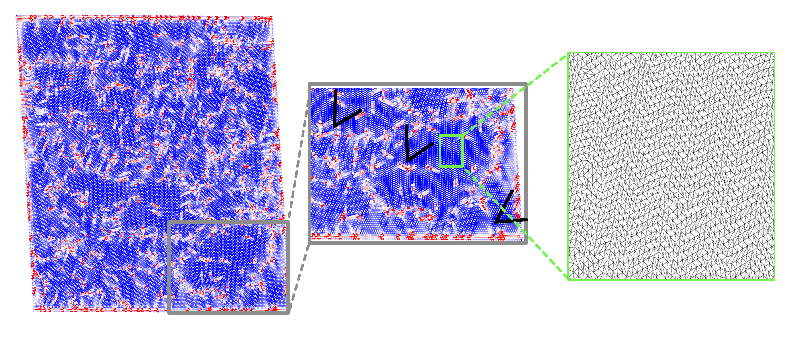
Figure 19: Post-avalanche pattern for a triangular lattice deformed along the simple shear loading path with $\theta=54$ degrees, see Eq. 12, which shows variously oriented dislocation-free grains

The observed differences in the character of the collective dislocation nucleation phenomenon along the ’hard’ loading paths in triangular and square lattices are probably related to the higher symmetry of the former. Thus, in triangular lattices due to the more ’compact’ structure of the effective yield surface, the instability of a homogeneous states takes place at lower levels of elastic energy which is then less available for the restructuring of the lattice. Therefore, instead of micro-twinning, aimed at the reduction of the energy globally, the system mimizes the energy locally by producing an intricate network of self-jammed dislocational entanglements. In other words the breakdown of metastability simply does not release enough energy to access the micro-twinned configuration, which requires major rearrangement.

Interestingly, our numerical experiments showed that using a specially designed loading protocol, the local micro-twinning can be achieved, see Fig. 19. Here one can see that the overall pseudo-rigid rotation inside a grain can be reached by complex micro-twinning which involves coexistence of the three unloaded triangular lattices corresponding to the bottoms of the energy wells, ${\bf T}$, ${\bf T}^{-1}_{2\pi/3}$ and ${\bf T}^{1}_{\pi/3}$, which are separated by semi-coherent grain boundaries oriented at either zero or 60 degrees, in accordance with the theoretical prediction made in our Appendix B.

5 Conclusions

In this paper we have presented new insights on homogeneous nucleation of dislocations in 2D pure crystals by emphasizing the collective nature of this phenomenon. These insights became possible due to the use of the novel mesoscopic tensorial model (MTM) of crystal plasticity which combines the advantages of pseudo-macroscopic description of plastic flows in terms of stresses and strains with the ability to describe short range interaction of dislocations and even resolve the crystallographic symmetry sensitive aspects of the structure of their cores. In contrast to some other mesoscopic approaches, the MTM does not require any dislocation-specific phenomenological entries and relies almost exclusively on the global symmetry of the lattice. This symmetry goes beyond the conventional point group and accounts in a geometrically exact way of lattice invariant shears.

The phenomenon of the homogeneous nucleation of dislocations presents a convenient background for testing the access of MTM to the crucial mesoscopic features of crystal plasticity. Previously, such nucleation in 2D was modeled as a localized event resulting in the formation of a topologically neutral pair of dislocations of opposite signs. Here we show that in the absence of defects and inhomogenities, the dislocation nucleation in pristine simple crystals unfolds as a system size avalanche. Due to the dominance of long range elastic interactions, it emerges as a collective phenomenon, involving a large number of dislocations, and leading to the formations of intricate patterns of global nature. We showed that some important peculiarities of such patterns may sensitively depend on the crystallographic symmetry of the lattice.

To highlight the importance of crystal symmetry in the process of homogeneous nucleation of dislocations we considered two main classes of simple lattices amenable to modeling in 2D: the lower symmetry square lattice and the higher symmetry triangular lattice. The possibility of defining general loading protocols allowed us to compare for both types of lattices the two archetypal loading paths: along the maximally ’soft’ direction and along the maximally ’hard’ direction.

Driving in the ’soft’ direction reveals a non-trivial coupling between several slip systems allowing the crystal to accommodate the applied loading by forming a relatively regular patterns of dislocation walls. The important role in such coupling is played by the metastable phases: triangular lattice ${\bf T}$ during the plasticity of square crystal $\bf S$ and vice versa. While in the case of plasticity of square crystal the implied branching of the energy valleys at the location of the triangular lattice $\bf T$ is immediately apparent, the situation is less simple in the case of plasticity of triangular crystals where the branching at the location of the square lattice $\bf S$ is between the different points of the orbit of the same lattice ${\bf T}^{1}_{\pi/3}\cong{\bf T}^{-1}_{0}$.

Instead, driving in a ’hard’ direction, produces in crystals with lower symmetry a regular pattern of mutually misoriented patches (or grains) where plastic deformation takes the form of micro-twinning disguised as rigid rotation [41]. Thus the collective nucleation of dislocation in the case of square crystals, ultimately resulting in a formation of laminates, proceeds through the propagation of a front. The latter involves the transverse motion of individual dislocations which are finally expelled to the boundary of the crystal leaving behind a fully unloaded but inelastically rotated original lattice. Such perfectly organized pattern fails to develop in triangular crystal, where it is replaced by a more complex network of jammed dislocation self-locks. Apparently, due to the higher symmetry of the crystal in this case, the dislocation generating instability takes place at the lower levels of stress which prevents global rearrangement replacing it with more local self-organization of individual slips.

Our exploratory study shows the strength of the MTM in dealing with the micro-structural aspects of crystal plasticity. This model can be potentially developed with no phenomenology at all if the periodic potential is constructed by ab initio methods. The natural future target of the model is the study of the mechanical fluctuations accompanying plastic yield. To be realistic the model should be moved from 2D to 3D where it should be able to reproduce the experimentally observed peculiarities of plastic fluctuations in FCC, BCC and HCP crystals.

6 Acknowledgments

The authors acknowledge helpful discussions with G. Zanzotto and C. Conti at the stage of the development of the MTM theory. O. U. S. is supported partially by the grant ANR-18-CE42-0017-03, O. U. S. and R.B. were supported by the grants ANR-19-CE08-0010-01, ANR-20-CE91- 0010, and L. T. by the grant ANR-10-IDEX-0001-02 PSL.

Appendix A Appendix: Numerical algorithm

1:Generation of finite element mesh of the body $\Omega$ and identification of boundary nodes on the boundary of the body $\partial\Omega$.

2:Initialization of the displacement vector $\bf u=0$ for all nodes $a$.

3:Set loading through the displacement ${\bf u}(\alpha)=(\bar{\bf F}(\alpha)-\mathbb{I}){\bf x}$ for all nodes $a$ on the boundary of the body $\partial\Omega$, where $\bar{\bf F}(\alpha)$ is the applied deformation gradient with amplitude $\alpha$.

4:Start the iterative L-FBGS minimization algorithm:

5: Construct a deformation gradient ${\bf F}$ in each finite element.

6: Construct a metric tensor ${\bf C}={\bf F}^{T}{\bf F}$ in each finite element.

7: Perform Lagrange reduction to calculate the reduced metric tensor ${\bf C}_{D}$ and the ${\bf m}$ matrix in each finite element.

8: Calculate the first Piola-Kirchhoff stress tensor.

9: Obtain nodal forces.

10: Obtain the total strain energy.

11: Obtain the new displacement vector $\bf u^{t}$ at iteration $t$ such that $W^{t}<W^{t-1}$

12: Ends minimization at iteration $t$ when $W^{t}-W^{t-1}<tol$

13:Start Newton algorithm with the displacement vector $\bf u^{t}$ obtained after the termination of L-FBGS minimisation algorithm

14: Construct a deformation gradient ${\bf F}$ in each finite element.

15: Construct a metric tensor ${\bf C}={\bf F}^{T}{\bf F}$ in each finite element.

16: Perform Lagrange reduction to calculate the reduced metric tensor ${\bf C}_{D}$ and the ${\bf m}$ matrix in each finite element.

17: Calculate the tensor $\bf A$.

18: Calculate the stiffness matrix $\bf K$ and the residual forces ${\bf R}$.

19: Perform a Newton step.

20: Obtain the new displacement vector $\bf u^{t}$ at iteration $t$ such that the vector norm of residual forces $|{\bf R}^{t}|<|{\bf R}^{t-1}|$.

21: Ends the Newton-Raphson at iteration $t$ when $|{\bf R}^{t}|-|{\bf R}^{t-1}|<tol$

22:Increase the loading amplitude: $\alpha\rightarrow\alpha+\delta\alpha$

23:Go to step 3

Appendix B Appendix: Twinning relations

Suppose that the constant deformation gradients $\bf G$ and $\bf H$ correspond to two equivalent minima of the strain-energy $\phi(\bf C)$. To generate piece wise affine continuous deformation, across an invariant discontinuity plane they must satisfy on such a plane the kinematic (Hadamard) compatibility conditions [54]:

$$\mathbf{R}\mathbf{H}=\mathbf{G}+\mathbf{a}\otimes\mathbf{n}^{*}=\mathbf{G}\left(\mathbf{I}+\mathbf{a}^{*}\otimes\mathbf{n}^{*}\right)=\left(\mathbf{I}+\mathbf{a}\otimes\mathbf{n}\right){\bf G}$$ (13)

where ${\bf R}\in SO(2)$ is a rotation. The Eulerian vector $\bf a$ (normal to the discontinuity plane) and covector $\bf n$ must satisfy ${\bf a}\cdot{\bf n}=0$; their Lagrangian counterparts are $\mathbf{a}^{*}=\mathbf{G}^{-1}\mathbf{a}$ and $\mathbf{n}^{*}=\mathbf{G}^{T}{\mathbf{n}}$. If we assume further that $\det\mathbf{H}=\det\mathbf{G}=1$ and exclude reflections, the deformation gradients satisfying (13) form a mechanical twin. If, in addition, the rotation $\mathbf{R}$ belongs to the point group of the lattice, such twinning structure produces the undistorted zero energy configuration. The resulting microtwinned laminates are sometimes referred to as pseudotwins [54].

The twinning equation (13) was studied extensively, see for instance [72]. It was shown that (13) admits either no solutions or two solutions. The two solutions exist when the matrix $\mathbf{G}^{-T}\mathbf{H}^{T}\mathbf{H}\mathbf{G}^{-1}\neq{\bf I}$ and its ordered eigenvalues $\mu_{1}<\mu_{2}$ are such that $\mu_{1}\mu_{2}=1$. In that case, the two solutions are given explicitly by the formulas:

$$\mathbf{a} =\rho\left(\sqrt{\frac{\mu_{2}(1-\mu_{1})}{\mu_{2}-\mu_{1}}}\mathbf{v}_{1}+\kappa\sqrt{\frac{\mu_{1}(\mu_{2}-1)}{\mu_{2}-\mu_{1}}}\mathbf{v}_{2}\right)\;,$$ (14)

$$\mathbf{n} =\frac{1}{\rho}\left(\frac{\sqrt{\mu_{2}}-\sqrt{\mu_{1}}}{\sqrt{\mu_{2}-\mu_{1}}}\right)\left(-\sqrt{1-\mu_{1}}\mathbf{v}_{1}+\kappa\sqrt{\mu_{2}-1}\mathbf{v}_{2}\right)\;,$$ (15)

where $\mathbf{\hat{v}}_{1}$ and $\mathbf{\hat{v}}_{2}$ are the normalized eigenvectors of $\mathbf{G}^{-T}\mathbf{H}^{T}\mathbf{H}\mathbf{G}^{-1}$, $\rho>0$ is a constant ensuring that $|{\bf n}|=1$ and $\kappa=\pm 1$. Once $\bf a$ and $\bf n$ are known, the rotation $\bf R$ can be obtained directly from (13).

First, we consider the compatibility of the two nearest wells reachable by deforming the original triangular phase using the deformation gradients:

1. ${\bf H}=\begin{pmatrix}1&\gamma^{2}\\ 0&1\end{pmatrix}$ and ${\bf G}=\begin{pmatrix}1&-\gamma^{2}\\ 0&1\end{pmatrix}.$ They correspond to the zero degree shear defined in Eq. 2 such that ${\bf H}={\bf F}(\gamma^{2},0)$ and ${\bf G}={\bf F}(-\gamma^{2},0)$.

2. ${\bf H}=\begin{pmatrix}1&\gamma^{2}\\ 0&1\end{pmatrix}$ and ${\bf G}=\begin{pmatrix}0.5&\sqrt{3}/6\\ -\sqrt{3}/2&1.5\end{pmatrix}$. The phase ${\bf G}$ is accesible by deforming the original triangular phase by ${\bf G}={\bf F}(-\gamma^{2},\pi/3)$.

3. ${\bf H}=\begin{pmatrix}0.5&\sqrt{3}/6\\ -\sqrt{3}/2&1.5\end{pmatrix}$ and ${\bf G}=\begin{pmatrix}0.5&-\sqrt{3}/6\\ \sqrt{3}/2&1.5\end{pmatrix}$. The phase ${\bf G}$ is accesible by deforming the original triangular phase by ${\bf G}={\bf F}(-\gamma^{2},2\pi/3)$.

4. ${\bf H}=\begin{pmatrix}1&-\gamma^{2}\\ 0&1\end{pmatrix}$ and ${\bf G}=\begin{pmatrix}0.5&-\sqrt{3}/6\\ \sqrt{3}/2&1.5\end{pmatrix}$.

We found that for each of the cases described above, the twinning equation admits solutions summarized below for each case:

1. Solution corresponding to $\kappa=1$ is given by

   $$\mathbf{a}^{T}=\{-1.74574,1.51186\}\quad\mathbf{n}^{T}=\{0.654654,0.755929\},$$ (16)

   and the corresponding rotation angle is 98.2132 degrees. . For $\kappa=-1$, the solution is different

   $$\mathbf{a}^{T}=\{-2.3094,0\}\quad\mathbf{n}^{T}=\{0,-1\}.$$ (17)

   We found that ${\bf R}=\mathds{1}$.

2. Solution corresponding to $\kappa=1$ is given by

   $$\mathbf{a}^{T}=\{0.436436,2.26779\}\quad\mathbf{n}^{T}=\{0.981981,-0.188982\},$$ (18)

   and the corresponding rotation angle is 38.2132 degrees.. For $\kappa=-1$, the solution is

   $$\mathbf{a}^{T}=\{-1.1547,2.\}\quad\mathbf{n}^{T}=\{-0.866025,-0.5\}.$$ (19)

   The corresponding rotation angle is $60$ degrees.

3. Solution corresponding to $\kappa=1$ is given by

   $$\mathbf{a}^{T}=\{1.1547005,2\}\quad\mathbf{n}^{T}=\{0.8660256,-0.5\},$$ (20)

   The corresponding rotation angle is $\pm 120$ degrees. The solution corresponding to $\kappa=-1$ is

   $$\mathbf{a}^{T}=\{-0.436436,2.26779\}\quad\mathbf{n}^{T}=\{-0.9819805,-0.188982\},$$ (21)

   The corresponding rotation angle is $21.7868$ degrees.

4. Solution corresponding to $\kappa=1$ is given by

   $$\mathbf{a}^{T}=\{1.1547005,2\}\quad\mathbf{n}^{T}=\{0.866025,-0.5\},$$ (22)

   The corresponding rotation angle is $60$ degrees. The solution corresponding to $\kappa=-1$ is

   $$\mathbf{a}^{T}=\{-0.436436,2.26779,\}\quad\mathbf{n}^{T}=\{-0.9819805,-0.188982\},$$ (23)

   the corresponding rotation angle is $38.2132$ degrees.

The results given above suggest that micro-twinning is possible in triangular lattices since there are several cases for which the rotation $\mathbf{R}$ belongs to the point group of the triangular lattice. However, as opposed to the case of square lattice, we did not observe any micro-twinning patterns in our numerical experiments in triangular lattices. One possible explanation is the strong misalignment, in the case of triangular lattices between the orientation of the macro-modulations and the lattice vectors when the critical loading is approached. Instead, in the case of square lattices we observe lattice scale modulations corresponding to the wave vectors at the boundary of the Brillouin zone present already in the original unstable mode, which is a perfect arrangement to generate a micro-laminate, see [18] for a detailed explanation on developing instability modes.

Second, we study the compatibility of the two nearest wells with the original triangular lattice that we take as identity ${\bf G}=\mathds{1}$. We have again 4 cases to consider (i) ${\bf H}=\begin{pmatrix}1&\gamma^{2}\\ 0&1\end{pmatrix}$, (ii) ${\bf H}=\begin{pmatrix}1&-\gamma^{2}\\ 0&1\end{pmatrix}$, (iii) ${\bf H}=\begin{pmatrix}0.5&\sqrt{3}/6\\ -\sqrt{3}/2&1.5\end{pmatrix}$, (iv) ${\bf H}=\begin{pmatrix}0.5&-\sqrt{3}/6\\ \sqrt{3}/2&1.5\end{pmatrix}$.

1. Solution corresponding to $\kappa=1$ is given by

   $$\mathbf{a}^{T}=\{0.57735,1.\}\quad\mathbf{n}^{T}=\{-0.866025,0.5\},$$ (24)

   and the corresponding rotation angle is 60 degrees. . For $\kappa=-1$, the solution is given by

   $$\mathbf{a}^{T}=\{1.1547,0\}\quad\mathbf{n}^{T}=\{0.,-1\}.$$ (25)

   We found that ${\bf R}=\mathds{1}$.

2. Solution corresponding to $\kappa=1$ is given by

   $$\mathbf{a}^{T}=\{-0.57735,1.\}\quad\mathbf{n}^{T}=\{0.866025,-0.5\},$$ (26)

   and the corresponding rotation angle is 60 degrees. . For $\kappa=-1$, the solution is given by

   $$\mathbf{a}^{T}=\{-1.1547,0\}\quad\mathbf{n}^{T}=\{0.,-1\}.$$ (27)

   We obtain ${\bf R}=\mathds{1}$.

3. Solution corresponding to $\kappa=1$ is given by

   $$\mathbf{a}^{T}=\{0.57735,1\}\quad\mathbf{n}^{T}=\{0.8660256,-0.5\},$$ (28)

   We obtain ${\bf R}=\mathds{1}$. The solution corresponding to $\kappa=-1$ is

   $$\mathbf{a}^{T}=\{-0.57735,1\}\quad\mathbf{n}^{T}=\{-0.8660256,-0.5\},$$ (29)

   The corresponding rotation angle is $60$ degrees.

4. Solution corresponding to $\kappa=1$ is given by

   $$\mathbf{a}^{T}=\{0.57735,1\}\quad\mathbf{n}^{T}=\{0.866025,-0.5\},$$ (30)

   The corresponding rotation angle is $60$ degrees. The solution corresponding to $\kappa=-1$ is

   $$\mathbf{a}^{T}=\{-0.57735,1\}\quad\mathbf{n}^{T}=\{-0.866025,-0.5\},$$ (31)

   the corresponding rotation is ${\bf R}=\mathds{1}$.

Bibliography

Bibliography

- [1] A. B. Movchan, R. Bullough, J. R. Willis, Stability of a dislocation : Discrete model, Eur. J. Appl. Math. 9 (4) (1998) 373–396.
- [2] V. Karlin, V. G. Maz’ya, A. B. Movchan, J. R. Willis, R. Bullough, Numerical solution of nonlinear hypersingular integral equations of the peierls type in dislocation theory, SIAM J. Appl. Math. 60 (2) (2000) 664–678.
- [3] A. A. Movchan, Phenomenological description of dislocation mechanism of defect nucleation during plastic deformation, 19 (5) PMTF. Zhurnal Prikladnoj Mekhaniki i Tekhnicheskoj (1987) 147–155.
- [4] R. Bullough, A.B. Movchan, J.R. Willis, The peierls-stress for various dislocation morphologies, Materials Modelling From Theory to Technology, CRC Press (1992).
- [5] A. B. Movchan, R. Bullough, J. R. Willis, Two-dimensional lattice models of the peierls type, Philos. Mag. 83 (5) (2003) 569–587.
- [6] P.-A. Geslin, R. Gatti, B. Devincre, D. Rodney, Implementation of the nudged elastic band method in a dislocation dynamics formalism: Application to dislocation nucleation, J. Mech. Phys. Solids 108 (2017) 49–67.
- [7] A. E. Mayer, Dislocation nucleation in al single crystal at shear parallel to 111 plane: Molecular dynamics simulations and nucleation theory with artificial neural networks, Int. J. Plast. 139 (2021) 102953.
- [8] E. T. Lilleodden, J. A. Zimmerman, S. M. Foiles, W. D. Nix, Atomistic simulations of elastic deformation and dislocation nucleation during nanoindentation, J. Mech. Phys. Solids 51 (5) (2003) 901–920.
- [9] J. K. Mason, A. C. Lund, C. A. Schuh, Determining the activation energy and volume for the onset of plasticity during nanoindentation, Phys. Rev. B Condens. Matter 73 (5) (2006) 054102.
- [10] S. Aubry, K. Kang, S. Ryu, W. Cai, Energy barrier for homogeneous dislocation nucleation: Comparing atomistic and continuum models, Scr. Mater. 64 (11) (2011) 1043–1046.
- [11] A. Asenjo, M. Jaafar, E. Carrasco, J. M. Rojo, Dislocation mechanisms in the first stage of plasticity of nanoindented au(111) surfaces, Phys. Rev. B Condens. Matter 73 (7) (2006) 075431.
- [12] P. Zhang, O. U. Salman, J. Weiss, L. Truskinovsky, Variety of scaling behaviors in nanocrystalline plasticity, Phys Rev E 102 (2-1) (2020) 023006.
- [13] V. Skogvoll, A. Skaugen, L. Angheluta, J. Viñals, Dislocation nucleation in the phase-field crystal model, Phys. Rev. B Condens. Matter 103 (1) (2021) 014107.
- [14] J. Li, The mechanics and physics of defect nucleation, MRS Bull. 32 (2) (2007) 151–159.
- [15] T. Zhu, J. Li, S. Ogata, S. Yip, Mechanics of Ultra-Strength materials, MRS Bull. 34 (3) (2009) 167–172.
- [16] X. Li, Y. Wei, L. Lu, K. Lu, H. Gao, Dislocation nucleation governed softening and maximum strength in nano-twinned metals, Nature 464 (7290) (2010) 877–880.
- [17] G. Grimvall, B. Magyari-Köpe, V. Ozoliņš, K. A. Persson, Lattice instabilities in metallic elements, Rev. Mod. Phys. 84 (2) (2012) 945–986.
- [18] O. U. Salman, R. Baggio, B. Bacroix, G. Zanzotto, N. Gorbushin, L. Truskinovsky, Discontinuous yielding of pristine micro-crystals, C. R. Phys. 22 (S3) (2021) 1–48.
- [19] M. A. Shehadeh, H. M. Zbib, On the homogeneous nucleation and propagation of dislocations under shock compression, Philos. Mag. 96 (26) (2016) 2752–2778.
- [20] E. M. Bringa, K. Rosolankova, R. E. Rudd, B. A. Remington, J. S. Wark, M. Duchaineau, D. H. Kalantar, J. Hawreliak, J. Belak, Shock deformation of face-centred-cubic metals on subnanosecond timescales, Nat. Mater. 5 (10) (2006) 805–809.
- [21] V. Bulatov, W. Cai, Computer Simulations of Dislocations, OUP Oxford, 2006.
- [22] M. Salvalaglio, L. Angheluta, Z.-F. Huang, A. Voigt, K. R. Elder, J. Viñals, A coarse-grained phase-field crystal model of plastic motion, J. Mech. Phys. Solids 137 (2020) 103856.
- [23] P. Y. Chan, G. Tsekenis, J. Dantzig, K. A. Dahmen, N. Goldenfeld, Plasticity and dislocation dynamics in a phase field crystal model, Phys. Rev. Lett. 105 (1) (2010) 015502.
- [24] V. B. Shenoy, R. Miller, E. b. Tadmor, D. Rodney, R. Phillips, M. Ortiz, An adaptive finite element approach to atomic-scale mechanics—the quasicontinuum method, J. Mech. Phys. Solids 47 (3) (1999) 611–642.
- [25] I. Plans, A. Carpio, L. L. Bonilla, Homogeneous nucleation of dislocations as bifurcations in a periodized discrete elasticity model, EPL 81 (3) (2007) 36001.
- [26] M. Javanbakht, V. I. Levitas, Phase field approach to dislocation evolution at large strains: Computational aspects, Int. J. Solids Struct. 82 (2016) 95–110.
- [27] J. Li, K. J. Van Vliet, T. Zhu, S. Yip, S. Suresh, Atomistic mechanisms governing elastic limit and incipient plasticity in crystals, Nature 418 (6895) (2002) 307–310.
- [28] K. J. Van Vliet, J. Li, T. Zhu, S. Yip, S. Suresh, Quantifying the early stages of plasticity through nanoscale experiments and simulations, Phys. Rev. B Condens. Matter 67 (10) (2003) 104105.
- [29] R. E. Miller, A. Acharya, A stress-gradient based criterion for dislocation nucleation in crystals, J. Mech. Phys. Solids 52 (7) (2004) 1507–1525.
- [30] A. Garg, A. Acharya, C. E. Maloney, A study of conditions for dislocation nucleation in coarser-than-atomistic scale models, J. Mech. Phys. Solids 75 (2015) 76–92.
- [31] T. J. Delph, J. A. Zimmerman, J. M. Rickman, J. M. Kunz, A local instability criterion for solid-state defects, J. Mech. Phys. Solids 57 (1) (2009) 67–75.
- [32] P. Schall, I. Cohen, D. A. Weitz, F. Spaepen, Visualizing dislocation nucleation by indenting colloidal crystals, Nature 440 (7082) (2006) 319–323.
- [33] M. A. Tschopp, D. E. Spearot, D. L. McDowell, Atomistic simulations of homogeneous dislocation nucleation in single crystal copper, Modell. Simul. Mater. Sci. Eng. 15 (7) (2007) 693.
- [34] R. E. Miller, D. Rodney, On the nonlocal nature of dislocation nucleation during nanoindentation, J. Mech. Phys. Solids 56 (4) (2008) 1203–1223.
- [35] R. J. Wagner, L. Ma, F. Tavazza, L. E. Levine, Dislocation nucleation during nanoindentation of aluminum, J. Appl. Phys. 104 (11) (2008) 114311.
- [36] A. Garg, C. E. Maloney, Universal scaling laws for homogeneous dislocation nucleation during nano-indentation, J. Mech. Phys. Solids 95 (2016) 742–754.
- [37] R. Baggio, E. Arbib, P. Biscari, S. Conti, L. Truskinovsky, G. Zanzotto, O. U. Salman, Landau-Type theory of planar crystal plasticity, Phys. Rev. Lett. 123 (20) (2019) 205501.
- [38] O. U. Salman, L. Truskinovsky, Minimal integer automaton behind crystal plasticity, Phys. Rev. Lett. 106 (17) (2011) 175503.
- [39] O. U. Salman, L. Truskinovsky, On the critical nature of plastic flow: One and two dimensional models, Int. J. Eng. Sci. 59 (2012) 219–254.
- [40] O. U. Salman, R. Baggio, Homogeneous Dislocation Nucleation in Landau Theory of Crystal Plasticity, Mechanics and Physics of Solids at Micro‐and Nano‐Scales, Wiley Online Library, 2019.
- [41] R. Baggio, O. U. Salman, L. Truskinovsky, Inelastic rotations and plastic turbulence, arXiv:2203.08711v3.
- [42] J. L. Ericksen, Nonlinear elasticity of diatomic crystals, Int. J. Solids Struct. 6 (7) (1970) 951–957.
- [43] J. L. Ericksen, The cauchy and born hypothesis for crystals, MRC Technical Summary Report.
- [44] I. Folkins, Functions of two‐dimensional bravais lattices, J. Math. Phys. 32 (7) (1991) 1965–1969.
- [45] G. P. Parry, Low‐Dimensional lattice groups for the continuum mechanics of phase transitions in crystals, Arch. Ration. Mech. Anal. 145 (1) (1998) 1–22.
- [46] S. Conti, G. Zanzotto, A variational model for reconstructive phase transformations in crystals, and their relation to dislocations and plasticity, Arch. Ration. Mech. Anal. 173 (1) (2004) 69–88.
- [47] C. Truesdell, W. Noll, The non-linear field theories of mechanics, in: The non-linear field theories of mechanics, Springer, 2004, pp. 1–579.
- [48] J. L. Ericksen, Special topics in elastostatics, in: Advances in applied mechanics, Vol. 17, Elsevier, 1977, pp. 189–244.
- [49] J. Ericksen, On the symmetry of deformable crystals, Arch. Ration. Mech. Anal 72 (1) (1979) 1–13.
- [50] J. Ericksen, Some phase transitions in crystals, Arch. Ration. Mech. Anal. 73 (2) (1980) 99–124.
- [51] J. L. Ericksen, Twinning of crystals (i), in: Metastability and incompletely posed problems, Springer, 1987, pp. 77–93.
- [52] J. Ericksen, Weak martensitic transformations in bravais lattices, in: Mechanics and Thermodynamics of Continua, Springer, 1991, pp. 145–158.
- [53] J. Ericksen, The cauchy and born hypotheses for crystals, Mechanics and mathematics of crystals: selected papers of JL Ericksen. Singapore: World Scientific Publishing Co (2005) 117–33.
- [54] M. Pitteri, G. Zanzotto, Continuum models for phase transitions and twinning in crystals, Chapman and Hall/CRC, 2002.
- [55] M. Pitteri, Reconciliation of local and global symmetries of crystals, J. Elast. 14 (2) (1984) 175–190.
- [56] A. Finel, Y. Le Bouar, A. Gaubert, U. Salman, Phase field methods: Microstructures, mechanical properties and complexity, C. R. Phys. 11 (3) (2010) 245–256.
- [57] O. U. Salman, B. Muite, A. Finel, Origin of stabilization of macrotwin boundaries in martensites, Eur. Phys. J. B 92 (1) (2019) 20.
- [58] P. Engel, Geometric crystallography: an axiomatic introduction to crystallography, Springer Science & Business Media, 2012.
- [59] M. Ortiz, R. Phillips, Nanomechanics of defects in solids, in: E. van der Giessen, T. Y. Wu (Eds.), Advances in Applied Mechanics, Vol. 36, Elsevier, 1998, pp. 1–79.
- [60] I. Fonseca, Variational methods for elastic crystals, Arch. Ration. Mech. Anal 97 (3) (1987) 189–220.
- [61] J. L. Ericksen, On the Cauchy—Born rule, Math. Mech. Solids 13 (3-4) (2008) 199–220.
- [62] S. Bochkanov, V. Bystritsky, Alglib, Available from: www alglib net.
- [63] C. Sanderson, R. Curtin, Armadillo: a template-based c++ library for linear algebra, J. Open Source Softw. 1 (2) (2016) 26.
- [64] C. Thiel, J. Voss, R. J. Martin, P. Neff, Shear, pure and simple, Int. J. Non Linear Mech. 112 (2019) 57–72.
- [65] R. W. Ogden, Non-linear elastic deformations, Courier Corporation, 1997.
- [66] R. Borja, Bifurcation of elastoplastic solids to shear band mode at finite strain, Comput. Methods Appl. Mech. Eng. 0 (0) (2001) 0.
- [67] J. R. Rice, Localization of plastic deformation, Tech. rep., Brown Univ., Providence, RI (USA). Div. of Engineering (1976).
- [68] Jaswon, El-Damanawi, What is a dislocation?, Math. Comput. Model.
- [69] Y. Kamimura, K. Edagawa, A. M. Iskandarov, M. Osawa, Y. Umeno, S. Takeuchi, Peierls stresses estimated via the Peierls-Nabarro model using ab-initio -surface and their comparison with experiments, Acta Mater. 148 (2018) 355–362.
- [70] V. V. Bulatov, E. Kaxiras, Semidiscrete variational peierls framework for dislocation core properties, Phys. Rev. Lett. 78 (22) (1997) 4221–4224.
- [71] A. S. K. Mohammed, O. K. Celebi, H. Sehitoglu, Critical stress prediction upon accurate dislocation core description, Acta Mater. 233 (2022) 117989.
- [72] A. Forclaz, A simple criterion for the existence of rank-one connections between martensitic wells, J. Elast. 57 (3) (1999) 281–305.