Celaya et al.

Proximity and flatness bounds for ILPs Proximity and flatness bounds for linear integer optimization

Marcel Celaya Department of Mathematics, Institute for Operations Research, ETH Zürich, Switzerland, marcel.celaya@ifor.math.ethz.ch Stefan Kuhlmann Institut für Mathematik, Technische Universität Berlin, Germany, kuhlmann@math.tu-berlin.de Joseph Paat Sauder School of Business, University of British Columbia, BC Canada, joseph.paat@sauder.ubc.ca Robert Weismantel Department of Mathematics, Institute for Operations Research, ETH Zürich, Switzerland, robert.weismantel@ifor.math.ethz.ch

This paper deals with linear integer optimization. We develop a technique that can be applied to provide improved upper bounds for two important questions in linear integer optimization.

• Proximity bounds: Given an optimal vertex solution for the linear relaxation, how far away is the nearest optimal integer solution (if one exists)?

• Flatness bounds: If a polyhedron contains no integer point, what is the smallest number of integer parallel hyperplanes defined by an integral, non-zero, normal vector that intersect the polyhedron?

This paper presents a link between these two questions by refining a proof technique that has been recently introduced by the authors. A key technical lemma underlying our technique concerns the areas of certain convex polygons in the plane: if a polygon $K\subseteq\mathbb{R}^{2}$ satisfies $\tau K\subseteq K^{\circ}$, where $\tau$ denotes $90^{\circ}$ counterclockwise rotation and $K^{\circ}$ denotes the polar of $K$, then the area of $K^{\circ}$ is at least 3.

1 Introduction.

Suppose $\boldsymbol{A}$ is an integral full-column-rank $m\times n$ matrix. By

$$\Delta_{k}\left(\boldsymbol{A}\right):=\max\left\{\left|\det\boldsymbol{M}\right|:\boldsymbol{M}\text{ is a $k\times k$ submatrix of $\boldsymbol{A}$}\right\}$$

we denote the largest absolute $k\times k$ minor of $\boldsymbol{A}$. The polyhedron corresponding to a right hand side $\boldsymbol{b}\in\mathbb{Q}^{m}$ is

$$\mathcal{P}\left(\boldsymbol{A},\boldsymbol{b}\right) :=\left\{\boldsymbol{x}\in\mathbb{R}^{n}:\ \boldsymbol{A}\boldsymbol{x}\leq\boldsymbol{b}\right\}.$$

The linear program corresponding to $$\mathcal{P}\left(\boldsymbol{A},\boldsymbol{b}\right) \boldsymbol{c}\in\mathbb{Q}^{n}$$ and an objective vector is

$$\operatorname{LP}(\boldsymbol{A},\boldsymbol{b},\boldsymbol{c}) :=\max\left\{\boldsymbol{c}^{\top}\boldsymbol{x}:\ \boldsymbol{x}\in\mathcal{P}\left(\boldsymbol{A},\boldsymbol{b}\right)\right\},$$

and the corresponding integer linear program is

$$\operatorname{IP}(\boldsymbol{A},\boldsymbol{b},\boldsymbol{c}) :=\max\left\{\boldsymbol{c}^{\top}\boldsymbol{x}:\ \boldsymbol{x}\in\mathcal{P}\left(\boldsymbol{A},\boldsymbol{b}\right)\cap\mathbb{Z}^{n}\right\}.$$

Our point of departure is the following foundational result due to Cook, Gerards, Schrijver, and Tardos that has several applications in integer optimization; see [6, 7, 15].

Theorem 1.1 (Theorem 1 in [4])

Let $\boldsymbol{b}\in\mathbb{Q}^{m}$ and $\boldsymbol{c}\in\mathbb{Q}^{n}$. Let $\boldsymbol{x}^{*}$ be an optimal vertex of $\operatorname{LP}(\boldsymbol{A},\boldsymbol{b},\boldsymbol{c})$. If $\operatorname{IP}(\boldsymbol{A},\boldsymbol{b},\boldsymbol{c})$ is feasible, then there exists an optimal solution $\boldsymbol{z}^{*}$ such that

$$\|\boldsymbol{x}^{*}-\boldsymbol{z}^{*}\|_{\infty}\leq n\cdot\Delta_{n-1}\left(\boldsymbol{A}\right).$$

The technique to prove Theorem 1.1 has been used to establish proximity bounds involving other data parameters [32] and different norms [19, 20]. Furthermore, their result has been extended to derive proximity results for convex separable programs [10, 14, 31] (where the bound in Theorem 1.1 remains valid), for mixed integer programs [25], and for random integer programs [24].

Lovász [28, Section 17.2] and Del Pia and Ma [5, Section 4] identified tuples $(\boldsymbol{A},\boldsymbol{b},\boldsymbol{c})$ such that proximity is arbitrarily close to the upper bound in Theorem 1.1. However, their examples crucially rely on the fact that $\boldsymbol{b}$ can take arbitrary rational values. In fact, Lovász’s example uses a totally unimodular matrix $\boldsymbol{A}$ while Del Pia and Ma use a unimodular matrix. Therefore, if the right hand sides $\boldsymbol{b}$ in their examples were to be replaced by the integral rounded down vector $\lfloor\boldsymbol{b}\rfloor$, then the polyhedron $\mathcal{P}(\boldsymbol{A},\lfloor\boldsymbol{b}\rfloor)$ would only have integral vertices. From an integer programming perspective, replacing $\boldsymbol{b}$ with $\lfloor\boldsymbol{b}\rfloor$ is natural as it strengthens the linear relaxation without cutting off any feasible integer solutions.

It remains an open question whether Cook et al.’s bound is tight when $\boldsymbol{b}\in\mathbb{Z}^{m}$. Under this assumption, Paat et al. [25] conjecture that the true bound is independent of $n$. This conjecture is supported by various results: Aliev et al. [2] prove that proximity is upper bounded by the largest entry of $\boldsymbol{A}$ for knapsack polytopes, Veselov and Chirkov’s result [30] implies a proximity bound of $2$ when $\Delta_{n}(\boldsymbol{A})\leq 2$, and Aliev et al. [1] prove a bound of $\Delta_{n}(\boldsymbol{A})$ for corner polyhedra.

One of our main results is an improvement on Theorem 1.1.

Theorem 1.2

Let $n\geq 2$, $\boldsymbol{b}\in\mathbb{Z}^{m}$, and $\boldsymbol{c}\in\mathbb{Q}^{n}$. Let $\boldsymbol{x}^{*}$ be an optimal vertex of $\operatorname{LP}(\boldsymbol{A},\boldsymbol{b},\boldsymbol{c})$. If $\operatorname{IP}(\boldsymbol{A},\boldsymbol{b},\boldsymbol{c})$ is feasible, then there exists an optimal solution $\boldsymbol{z}^{*}$ such that

$$\|\boldsymbol{x}^{*}-\boldsymbol{z}^{*}\|_{\infty}<\frac{4n+2}{9}\cdot\Delta_{n-1}(\boldsymbol{A}).$$

A second equally fundamental question in discrete mathematics is concerned with bounds on flatness of $\mathcal{P}(\boldsymbol{A},\boldsymbol{b})$ if $\mathcal{P}(\boldsymbol{A},\boldsymbol{b})$ is lattice-free, i.e., $\mathcal{P}(\boldsymbol{A},\boldsymbol{b})\cap\mathbb{Z}^{n}=\emptyset$. The width of $\mathcal{P}\left(\boldsymbol{A},\boldsymbol{b}\right)$ in direction $\boldsymbol{a}\in\mathbb{R}^{n}\backslash\{0\}$ is defined by

$$w^{\boldsymbol{a}}\left(\mathcal{P}\left(\boldsymbol{A},\boldsymbol{b}\right)\right):=\max_{\boldsymbol{x}\in\mathcal{P}\left(\boldsymbol{A},\boldsymbol{b}\right)}\boldsymbol{a}^{\top}\boldsymbol{x}-\min_{\boldsymbol{y}\in\mathcal{P}\left(\boldsymbol{A},\boldsymbol{b}\right)}\boldsymbol{a}^{\top}\boldsymbol{y}.$$

The lattice width is defined by

$$w\left(\mathcal{P}\left(\boldsymbol{A},\boldsymbol{b}\right)\right):=\min_{\boldsymbol{a}\in\mathbb{Z}^{n}\backslash\{\mathbf{0}\}}w^{\boldsymbol{a}}\left(\mathcal{P}\left(\boldsymbol{A},\boldsymbol{b}\right)\right).$$

A prominent result regarding the lattice width is due to Khinchine.

Theorem 1.3 ([18])

Let $\mathcal{P}\left(\boldsymbol{A},\boldsymbol{b}\right)$ be a lattice-free polyhedron. There exists a non-zero vector $\boldsymbol{a}\in\mathbb{Z}^{n}$ such that $w^{\boldsymbol{a}}\left(\mathcal{P}\left(\boldsymbol{A},\boldsymbol{b}\right)\right)$ is bounded above by some function depending only on the dimension $n$.

The current best upper bound is $\mathcal{O}^{*}(n^{\frac{4}{3}})$, where $\mathcal{O}^{*}$ denotes that a polynomial in $\log n$ is omitted; see [26]. It is conjectured that the lattice width can be bounded by a function which only depends linearly on $n$.

A variety of algorithms related to integer programs rely on upper bounds on the lattice width of lattice-free polytopes. One famous example is Lenstra’s approach to solve the feasibility question of integer linear programs [21]. In order to improve the understanding of the running time of these algorithms with respect to their input, it is a natural task to analyze the lattice width in dependence of other input parameters than $n$.

Gribanov and Veselov presented the first bound on the lattice width of lattice-free polytopes which depends linearly on $n$ and on the least common multiple of all $n\times n$ minors; see [11]. The least common multiple is in the worst case exponentially large in $\Delta_{n}(\boldsymbol{A})$. We present a bound that depends linearly on $n$ and linearly on $\Delta_{n}(\boldsymbol{A})$.

Theorem 1.4

Let $n\geq 2$ and $\boldsymbol{b}\in\mathbb{Z}^{m}$ such that $\mathcal{P}\left(\boldsymbol{A},\boldsymbol{b}\right)$ is a full-dimensional lattice-free polyhedron and each row of $\boldsymbol{A}$ is facet-defining. Then, there exists a row $\boldsymbol{a}$ of $\boldsymbol{A}$ such that

$$w^{\mathcal{\boldsymbol{a}}}\left(\mathcal{P}\left(\boldsymbol{A},\boldsymbol{b}\right)\right)<\frac{4n+2}{9}\cdot\Delta_{n}(\boldsymbol{A})-1.$$

It is open whether the lattice width of lattice-free polytopes can be bounded solely by $\Delta_{n}(\boldsymbol{A})$. Some interesting classes of polytopes, where this is the case, are simplices and special pyramids; see [13]. In [17], the authors utilize bounds on the facet width of certain lattice-free polytopes with respect to their minors to construct an algorithm which efficiently enumerates special integer vectors in those polytopes.

On the first glance Theorem 1.2 and 1.4 have nothing in common. However, we will show that both results follow from a more general result that allows us to establish a bound on the gap of the value between a linear optimization problem and its integer analogue. This applies to arbitrary integral valued objective function vectors. In order to state this result formally, let us introduce the following definition.

Definition 1.5

Let $\boldsymbol{A}\in\mathbb{Z}^{m\times n}$ be full-column-rank matrix. For $\boldsymbol{\alpha}\in\mathbb{Z}^{n}$, let

$$\Delta^{\boldsymbol{\alpha}}\left(\boldsymbol{A}\right):=\max\left\{\left|\det\left(\begin{array}[]{l}\boldsymbol{\alpha}^{\top}\\ \boldsymbol{B}\end{array}\right)\right|:\boldsymbol{B}\text{ is a }(n-1)\times n\text{ submatrix of }\boldsymbol{A}\right\}.$$

Theorem 1.6

Let $\boldsymbol{\alpha}\in\mathbb{Z}^{n}\backslash\{\mathbf{0}\}$, $n\geq 2$, $\boldsymbol{b}\in\mathbb{Z}^{m}$, and $\boldsymbol{c}\in\mathbb{Q}^{n}$. Let $\boldsymbol{x}^{*}$ be an optimal vertex of $\operatorname{LP}(\boldsymbol{A},\boldsymbol{b},\boldsymbol{c})$. If $\operatorname{IP}(\boldsymbol{A},\boldsymbol{b},\boldsymbol{c})$ is feasible, then there exists an optimal solution $\boldsymbol{z}^{*}$ such that

$$\left|\boldsymbol{\alpha}^{\top}(\boldsymbol{x}^{*}-\boldsymbol{z}^{*})\right|<\frac{4n+2}{9}\cdot\Delta^{\boldsymbol{\alpha}}\left(\boldsymbol{A}\right).$$

Our proof of Theorem 1.6 consists of three major parts. First, we apply a dimension reduction technique so that general instances can be reduced to full-dimensional instances in lower dimensional space. This is discussed in Section 3. Next, we establish a relationship between Theorem 1.6 and the volume of a particular polytope associated with the matrix $\boldsymbol{A}$ and the vector $\boldsymbol{\alpha}$. This applies to arbitrary dimensions. In order to give an estimate on the volume, we restrict our attention to low dimensional cases. We establish such lower bounds when $n=1$ and $n=2$; see the end of Section 3. Third, we show how these bounds in lower dimensions can be lifted to bounds in higher dimensions; see Section 5. Section 4 is devoted to carrying out the calculations when $n=3$.

When $n=3$, this particular polytope transforms linearly into a polygon $\mathcal{Q}^{\circ}\subseteq\mathbb{R}^{2}$ satisfying $\tau\mathcal{Q}\subseteq\mathcal{Q}^{\circ}$, where $\tau$ denotes the $90^{\circ}$ counterclockwise rotation. In Appendix 9, we show that the area of any such polygon is at least 3. For this we show that it is sufficient to consider the extremal case where $\tau\mathcal{Q}=\mathcal{Q}^{\circ}$. Polytopes of this type have been analysed by Jensen in [16] (see also [9] for the planar case), where they are called self-polar polytopes. Next, by repeatedly applying Jensen’s add-and-cut modification described in [16], we show all minimal-area polygons $\mathcal{Q}$ satisfying $\tau\mathcal{Q}=\mathcal{Q}^{\circ}$ have area 3. We remark that inequalities relating the volume of a polytope with the volume of its polar have long been investigated; their product is the subject of Mahler’s conjecture [22] (see also [12, Page 177]), and their sum has been studied in the planar case [8].

Our techniques can be adapted to analyze the special case when the $n\times n$ minors of $\boldsymbol{A}$ are contained in $\{0,\pm k,\pm 2k\}$ for some integer $k\geq 1$. A special instance of such a matrix $\boldsymbol{A}$ is the case when $\boldsymbol{A}$ is strictly $\Delta_{n}(\boldsymbol{A})$-modular, that is, $\boldsymbol{A}=\boldsymbol{T}\boldsymbol{B}$ for a totally unimodular matrix $\boldsymbol{T}$ and a square integer matrix $\boldsymbol{B}$ with determinant $\Delta_{n}(\boldsymbol{A})$. In this case, the bounds on proximity and flatness are independent of the dimension, generalizing results of Nägele, Santiago, and Zenklusen [23, Theorem 1.4 and 1.5].

Theorem 1.7

Let the $n\times n$ minors of $\boldsymbol{A}$ be contained in $\{0,\pm k,\pm 2k\}$ for some integer $k\geq 1$. The following hold:

1. The bound in Theorem 1.2 can be sharpened to

   $$\|\boldsymbol{x}^{*}-\boldsymbol{z}^{*}\|_{\infty}\leq\max\{\Delta_{n-1}(\boldsymbol{A}),\Delta_{n}(\boldsymbol{A})\}-1$$

   and

   $$\|\boldsymbol{x}^{*}-\boldsymbol{z}^{*}\|_{\infty}<\Delta_{n-1}(\boldsymbol{A}).$$

2. The bound in Theorem 1.4 can be sharpened to

   $$w^{\mathcal{\boldsymbol{a}}}\left(\mathcal{P}\left(\boldsymbol{A},\boldsymbol{b}\right)\right)\leq\Delta_{n}(\boldsymbol{A})-2.$$

The proof of this theorem is given in Section 8.

Remark 1.8

This manuscript builds upon the work carried out by the authors in [3]. All of the results in this paper are strict improvements of the results in [3], with the main new contributions being the improved constant in Theorem 1.2, the flatness result of Theorem 1.4, and the extension of Theorem 1.7 to the $\{0,\pm k,\pm 2k\}$-setting. $\diamond$

2 Basic Definitions and Notation.

Here we outline the key objects and parameters used in the paper.

Let $\boldsymbol{A}\in\mathbb{Z}^{m\times n}$ be a full-column-rank matrix, and $\boldsymbol{b}\in\mathbb{Z}^{m}$ be such that $\mathcal{P}(\boldsymbol{A},\boldsymbol{b})\cap\mathbb{Z}^{n}\neq\emptyset$. For $I\subseteq[m]:=\{1,\ldots,m\}$, we use $\boldsymbol{A}_{I}$ and $\boldsymbol{b}_{I}$ to denote the rows of $\boldsymbol{A}$ and $\boldsymbol{b}$ indexed by $I$. If $I=\{i\}$, then we write $\boldsymbol{a}_{i}^{\top}:=\boldsymbol{A}_{I}$. We use $\mathbf{0}$ and $\mathbf{1}$ to denote the all zero and all one vector (in appropriate dimension). For a polyhedron $\mathcal{Q}\subseteq\mathbb{R}^{n}$, the dimension of $\mathcal{Q}$ is the dimension of the linear span of $\mathcal{Q}$ and is denoted by $\dim\mathcal{Q}$. We also define, for $I\subseteq[m]$,

$$\gcd\boldsymbol{A}_{I}:=\gcd\left\{\left|\det\boldsymbol{M}\right|:\ \boldsymbol{M}~{}\text{is a}~{}\text{rank}(\boldsymbol{A}_{I})\times\text{rank}(\boldsymbol{A}_{I})~{}\text{submatrix of}~{}\boldsymbol{A}_{I}\right\},$$

with $\gcd\boldsymbol{A}_{\emptyset}=1$. In the case when $\mathcal{P}\cap\mathbb{Z}^{n}=\{\mathbf{0}\}$, bounding proximity is equivalent to bounding

$$\max_{\boldsymbol{x}\in\mathcal{P}(\boldsymbol{A},\boldsymbol{b})}\ \|\boldsymbol{x}\|_{\infty}=\max_{\boldsymbol{\alpha}\in\{\pm\mathbf{e}_{1},\ldots,\pm\mathbf{e}_{n}\}}\ \max\left\{\boldsymbol{\alpha}^{\top}\boldsymbol{x}:\ \boldsymbol{x}\in\mathcal{P}(\boldsymbol{A},\boldsymbol{b})\right\},$$ (1)

where $\mathbf{e}_{1},\ldots,\mathbf{e}_{n}\in\mathbb{Z}^{n}$ are the standard unit vectors. As we shall see in the proof of Theorem 1.6, the general case then follows from this case. In light of this, we analyze the maximum of an arbitrary linear form $\boldsymbol{\alpha}^{\top}\boldsymbol{x}$ over $\mathcal{P}(\boldsymbol{A},\boldsymbol{b})$ for $\boldsymbol{\alpha}\in\mathbb{Z}^{n}$.

We provide non-trivial bounds on the maximum of these linear forms for small values of $n$; see Section 3 and 4. In order to lift low dimensional results to higher dimensions (see Section 5), we consider slices of $\mathcal{P}\left(\boldsymbol{A},\boldsymbol{b}\right)$ through the origin induced by rows of $\boldsymbol{A}$. Given $I\subseteq\left[m\right]$ such that $|I|\leq n-1$ and $\text{rank}~{}\boldsymbol{A}_{I}=|I|$, define

$$\mathcal{P}_{I}\left(\boldsymbol{A},\boldsymbol{b}\right):=\mathcal{P}\left(\boldsymbol{A},\boldsymbol{b}\right)\cap\ker\boldsymbol{A}_{I}.$$

We specify $\ker\boldsymbol{A}_{\emptyset}=\mathbb{R}^{n}$, so that $\mathcal{P}_{\emptyset}(\boldsymbol{A},\boldsymbol{b})=\mathcal{P}(\boldsymbol{A},\boldsymbol{b})$. The bounds that we provide on $\boldsymbol{\alpha}^{\top}\boldsymbol{x}$ are given in terms of the parameter

$$\Delta^{\boldsymbol{\alpha}}_{I}\left(\boldsymbol{A}\right):=\frac{1}{\gcd\boldsymbol{A}_{I}}\cdot\max\left\{\left|\det\left(\begin{array}[]{c}\boldsymbol{\alpha}^{\top}\\ \boldsymbol{A}_{K}\end{array}\right)\right|:I\subseteq K\subseteq\left[m\right],\;\left|K\right|=n-1\right\}.$$

Observe that $\Delta^{\boldsymbol{\alpha}}\left(\boldsymbol{A}\right)=\Delta^{\boldsymbol{\alpha}}_{\emptyset}(\boldsymbol{A})$. In particular, we define $\kappa_{I}\left(\boldsymbol{A},\boldsymbol{b},\boldsymbol{\alpha}\right)$ to be the number satisfying

$$\max_{\boldsymbol{x}\in\mathcal{P}_{I}\left(\boldsymbol{A},\boldsymbol{b}\right)}\boldsymbol{\alpha}^{\top}\boldsymbol{x}=\kappa_{I}\left(\boldsymbol{A},\boldsymbol{b},\boldsymbol{\alpha}\right)\Delta^{\boldsymbol{\alpha}}_{I}\left(\boldsymbol{A}\right).$$ (2)

Maximizing over all $I\subseteq\left[m\right]$ such that $\mathcal{P}_{I}\left(\boldsymbol{A},\boldsymbol{b}\right)$ has a fixed dimension $d$, define

$$\kappa_{d}\left(\boldsymbol{A},\boldsymbol{b},\boldsymbol{\alpha}\right):=\max_{I:\dim\mathcal{P}_{I}\left(\boldsymbol{A},\boldsymbol{b}\right)=d}\kappa_{I}\left(\boldsymbol{A},\boldsymbol{b},\boldsymbol{\alpha}\right).$$

Equation (2) looks similar to the bound we seek. However, $\Delta^{\boldsymbol{\alpha}}_{I}\left(\boldsymbol{A}\right)$ depends on $\boldsymbol{\alpha}$, whereas our main result (Theorem 1.2) only depends on $\Delta_{n-1}(\boldsymbol{A})$. Later (see Section 6), we will substitute $\pm\mathbf{e}_{1},\ldots,\pm\mathbf{e}_{n}$ in for $\boldsymbol{\alpha}$ as in (1). We also want to consider $I=\emptyset$ because $\mathcal{P}_{\emptyset}(\boldsymbol{A},\boldsymbol{b})=\mathcal{P}(\boldsymbol{A},\boldsymbol{b})$ by definition. Note that when $\boldsymbol{\alpha}$ is a unit vector, then $\Delta^{\boldsymbol{\alpha}}_{I}\left(\boldsymbol{A}\right)$ is a lower bound for $\Delta_{n-1}(\boldsymbol{A})$. Another important object for us is the following cone. For $\boldsymbol{x}^{*}\in\mathbb{R}^{n}$, define

$$\mathcal{C}\left(\boldsymbol{A},\boldsymbol{x}^{*}\right):=\left\{\boldsymbol{x}\in\mathbb{R}^{n}:\begin{array}[]{rl}\mathrm{sign}\left(\boldsymbol{a}_{i}^{\top}\boldsymbol{x}^{*}\right)\cdot\boldsymbol{a}_{i}^{\top}\boldsymbol{x}&\geq 0~{}\forall~{}i\in[m]~{}\text{such that}~{}\boldsymbol{a}_{i}^{\top}\boldsymbol{x}^{*}\neq 0\\[2.84544pt] \boldsymbol{a}_{i}^{\top}\boldsymbol{x}&=0~{}\forall~{}i\in[m]~{}\text{such that}~{}\boldsymbol{a}_{i}^{\top}\boldsymbol{x}^{*}=0\end{array}\right\}.$$

The cone $\mathcal{C}\left(\boldsymbol{A},\boldsymbol{x}^{*}\right)$ serves as a key ingredient in the proof of Theorem 1.1 in [4]. We also define the polytope

$$\mathcal{S}\left(\boldsymbol{A},\boldsymbol{x}^{*}\right):=\mathcal{C}\left(\boldsymbol{A},\boldsymbol{x}^{*}\right)\cap\left(\boldsymbol{x}^{*}-\mathcal{C}\left(\boldsymbol{A},\boldsymbol{x}^{*}\right)\right).$$

One checks that if $\boldsymbol{x}^{*}\in\mathcal{P}\left(\boldsymbol{A},\boldsymbol{b}\right)$, then $\mathcal{S}\left(\boldsymbol{A},\boldsymbol{x}^{*}\right)\subseteq\mathcal{P}\left(\boldsymbol{A},\boldsymbol{b}\right)$. Moreover, if $\boldsymbol{y}^{*}\in\mathcal{S}\left(\boldsymbol{A},\boldsymbol{x}^{*}\right)$ then $\mathcal{S}\left(\boldsymbol{A},\boldsymbol{y}^{*}\right)\subseteq\mathcal{S}\left(\boldsymbol{A},\boldsymbol{x}^{*}\right)$. Polytopes of this form, namely, ones in which every facet is incident to one of two distinguished vertices, known as spindles, were used in [27] to construct counterexamples to the Hirsch conjecture.

We often fix $\boldsymbol{A}\in\mathbb{Z}^{m\times n}$ and $\boldsymbol{b}\in\mathbb{Z}^{m}$. Thus, if the dependence on $\boldsymbol{A}$ and $\boldsymbol{b}$ is clear from the context, we abbreviate $\mathcal{P}_{I}$ for $\mathcal{P}_{I}(\boldsymbol{A},\boldsymbol{b})$, $\Delta^{\boldsymbol{\alpha}}_{I}$ for $\Delta^{\boldsymbol{\alpha}}_{I}\left(\boldsymbol{A}\right)$, $\kappa(\boldsymbol{\alpha})$ for $\kappa(\boldsymbol{A},\boldsymbol{b},\boldsymbol{\alpha})$, $\mathcal{S}(\boldsymbol{x}^{*})$ for $\mathcal{S}(\boldsymbol{A},\boldsymbol{x}^{*})$ and so on.

3 Dimension Reduction and Further Preliminaries.

A useful fact for us is that we only need to consider the case when $\dim\mathcal{P}=n$, by replacing a not-necessarily full-dimensional instance with an equivalent full-dimensional instance in a lower-dimensional space. This construction is outlined below.

Lemma 3.1

Let $\boldsymbol{\alpha}\in\mathbb{Z}^{n}$ such that $\max\{\boldsymbol{\alpha}^{\top}\boldsymbol{x}:\boldsymbol{x}\in\mathcal{P}\}$ is attained and is finite. Assume $I\subseteq\left[m\right]$ determines a linearly independent subset of the rows of $\boldsymbol{A}$ such that the linear span of $\mathcal{P}_{I}$ is $\ker\boldsymbol{A}_{I}$, which has dimension $d$. Then there exists a linear isomorphism $\ker\boldsymbol{A}_{I}\rightarrow\mathbb{R}^{d}$ given by $\boldsymbol{x}\mapsto\boldsymbol{P}\boldsymbol{x}$ where $\boldsymbol{P}\in\mathbb{Z}^{d\times n}$, which maps $\ker\boldsymbol{A}_{I}\cap\mathbb{Z}^{n}$ onto $\mathbb{Z}^{d}$ and maps $\mathcal{P}_{I}(\boldsymbol{A},\boldsymbol{b})$ onto $\mathcal{P}(\hat{\boldsymbol{A}\;}\negthickspace,\hat{\boldsymbol{b}})$ for some $\hat{\boldsymbol{A}\;}\negthickspace\in\mathbb{Z}^{\left(m-n+d\right)\times d}$, $\hat{\boldsymbol{b}}\in\mathbb{Z}^{m-n+d}$, and satisfies

$$\kappa_{I}\left(\boldsymbol{A},\boldsymbol{b},\boldsymbol{\alpha}\right)=\kappa_{d}\bigl{(}\hat{\boldsymbol{A}\;}\negthickspace,\hat{\boldsymbol{b}},\hat{\boldsymbol{\alpha}}\bigr{)}$$

where $\hat{\boldsymbol{\alpha}}\in\mathbb{Z}^{d}$ is the unique vector satisfying $\hat{\boldsymbol{\alpha}}^{\top}\boldsymbol{P}=\boldsymbol{\alpha}^{\top}$.

Proof 3.2

Proof. Without loss of generality, suppose $I=[n-d]$. Set $J:=[n-d]$, $\bar{J}:=\{n-d+1,\ldots,n\}$, and $\bar{I}:=\{n-d+1,\ldots,m\}$. Choose a unimodular matrix $\boldsymbol{U}\in\mathbb{Z}^{n\times n}$ (e.g., via the Hermite Normal Form of $\boldsymbol{A}_{[n]}$) such that

$$\boldsymbol{A}\boldsymbol{U}=\begin{pmatrix}\left(\boldsymbol{A}\boldsymbol{U}\right)_{I,J}&\mathbf{0}\\ \left(\boldsymbol{A}\boldsymbol{U}\right)_{\bar{I},J}&\left(\boldsymbol{A}\boldsymbol{U}\right)_{\bar{I},\bar{J}}\end{pmatrix}$$

with $\left(\boldsymbol{A}\boldsymbol{U}\right)_{I,J}$ square and invertible.

Set $\hat{\boldsymbol{A}\;}\negthickspace:=\left(\boldsymbol{A}\boldsymbol{U}\right)_{\bar{I},\bar{J}},$ $\hat{\boldsymbol{b}}:=\boldsymbol{b}_{\bar{I}},$ and $\hat{\boldsymbol{\alpha}}^{\top}:=\left(\boldsymbol{\alpha}^{\top}\boldsymbol{U}\right)_{\bar{J}}.$ For $\boldsymbol{x}\in\ker\boldsymbol{A}_{I}$, we have

$$\mathbf{0}=\boldsymbol{A}_{I}\boldsymbol{x}=\boldsymbol{A}_{I}\boldsymbol{U}\boldsymbol{U}^{-1}\boldsymbol{x}=[(\boldsymbol{A}\boldsymbol{U})_{I,J}~{}\mathbf{0}]\ \boldsymbol{U}^{-1}\boldsymbol{x}=(\boldsymbol{A}\boldsymbol{U})_{I,J}(\boldsymbol{U}^{-1}\boldsymbol{x})_{J}.$$

Thus, $(\boldsymbol{U}^{-1}\boldsymbol{x})_{J}=\mathbf{0}$. Hence, the map $\boldsymbol{x}\mapsto\left(\boldsymbol{U}^{-1}\boldsymbol{x}\right)_{\bar{J}}$ is a linear isomorphism from $\ker\boldsymbol{A}_{I}$ to $\mathbb{R}^{|\bar{J}|}=\mathbb{R}^{d}$, which restricts to a lattice isomorphism from $\ker\boldsymbol{A}_{I}\cap\mathbb{Z}^{n}$ to $\mathbb{Z}^{d}$ and maps $\mathcal{P}_{I}(\boldsymbol{A},\boldsymbol{b})$ to $\mathcal{P}\bigl{(}\hat{\boldsymbol{A}\;}\negthickspace,\hat{\boldsymbol{b}}\bigr{)}$. It follows that $\mathcal{P}\bigl{(}\hat{\boldsymbol{A}\;}\negthickspace,\hat{\boldsymbol{b}}\bigr{)}\cap\mathbb{Z}^{d}=\left\{\mathbf{0}\right\}$. For $\boldsymbol{x}\in\ker\boldsymbol{A}_{I}$, the equation $\left(\boldsymbol{U}^{-1}\boldsymbol{x}\right)_{J}=\mathbf{0}$ implies that

$$\boldsymbol{\alpha}^{\top}\boldsymbol{x}=\boldsymbol{\alpha}^{\top}\boldsymbol{U}\boldsymbol{U}^{-1}\boldsymbol{x}=\hat{\boldsymbol{\alpha}}^{\top}\left(\boldsymbol{U}^{-1}\boldsymbol{x}\right)_{\bar{J}}.$$ (3)

Moreover, if $K\subseteq\bar{I}$ with $\left|K\right|=d-1$, then

$$\left|\det\left(\begin{array}[]{c}\hat{\boldsymbol{\alpha}}^{\top}\\ \hat{\boldsymbol{A}\;}\negthickspace_{K}\end{array}\right)\right| =\left|\det\left(\begin{array}[]{r@{\hskip 0 cm}r@{\hskip 0 cm}l}\left(\right.\hskip 0.0pt&\boldsymbol{\alpha}^{\top}\boldsymbol{U}\hskip 0.0pt&\left.\right)_{\bar{J}}\\ \left(\right.\hskip 0.0pt&\boldsymbol{A}\boldsymbol{U}\hskip 0.0pt&\left.\right)_{K,\bar{J}}\end{array}\right)\right|$$

$$=\frac{1}{\bigl{|}\det\left(\boldsymbol{A}\boldsymbol{U}\right)_{I,J}\bigr{|}}\cdot\left|\det\left(\begin{array}[]{r@{\hskip 0 cm}r@{\hskip 0 cm}lr@{\hskip 0 cm}r@{\hskip 0 cm}l}\left(\right.\hskip 0.0pt&\boldsymbol{A}\boldsymbol{U}\hskip 0.0pt&\left.\right)_{I,J}&\hskip 0.0pt&\mathbf{0}{}{}\hskip 0.0pt&\\ \left(\right.\hskip 0.0pt&\boldsymbol{\alpha}^{\top}\boldsymbol{U}\hskip 0.0pt&\left.\right)_{J}&\left(\right.\hskip 0.0pt&\boldsymbol{\alpha}^{\top}\boldsymbol{U}\hskip 0.0pt&\left.\right)_{\bar{J}}\\ \left(\right.\hskip 0.0pt&\boldsymbol{A}\boldsymbol{U}\hskip 0.0pt&\left.\right)_{K,J}&\left(\right.\hskip 0.0pt&\boldsymbol{A}\boldsymbol{U}\hskip 0.0pt&\left.\right)_{K,\bar{J}}\end{array}\right)\right|$$

$$=\frac{1}{\gcd\boldsymbol{A}_{I}}\cdot\left|\det\left(\begin{array}[]{c}\boldsymbol{\alpha}^{\top}\\ \boldsymbol{A}_{I\cup K}\end{array}\right)\right|,$$

where we have used $\bigl{|}\det\left(\boldsymbol{A}\boldsymbol{U}\right)_{I,J}\bigr{|}=\gcd(\boldsymbol{A}\boldsymbol{U})_{I}=\gcd\boldsymbol{A}_{I}\boldsymbol{U}=\gcd\boldsymbol{A}_{I}.$ Taking the maximum over all such $K$, we get

$$\Delta^{\hat{\boldsymbol{\alpha}}}(\hat{\boldsymbol{A}\;}\negthickspace)=\Delta^{\boldsymbol{\alpha}}_{I}\left(\boldsymbol{A}\right).$$ (4)

Putting (3) and (4) together, we get

$$\kappa_{d}\bigl{(}\hat{\boldsymbol{A}\;}\negthickspace,\hat{\boldsymbol{b}},\hat{\boldsymbol{\alpha}}\bigr{)}=\max_{\boldsymbol{y}\in\mathcal{P}\left(\hat{\boldsymbol{A}\;}\negthickspace,\hat{\boldsymbol{b}}\right)}\ \frac{\hat{\boldsymbol{\alpha}}^{\top}\boldsymbol{y}}{\Delta^{\hat{\boldsymbol{\alpha}}}(\hat{\boldsymbol{A}\;}\negthickspace)}=\max_{\boldsymbol{x}\in\mathcal{P}_{I}(\boldsymbol{A},\boldsymbol{b})}\ \frac{\boldsymbol{\alpha}^{\top}\boldsymbol{x}}{\Delta^{\boldsymbol{\alpha}}_{I}\left(\boldsymbol{A}\right)}=\kappa_{I}\left(\boldsymbol{A},\boldsymbol{b},\boldsymbol{\alpha}\right).$$

Next, we present a general relationship between the volume of polyhedra associated with the matrix $\boldsymbol{A}$, $\boldsymbol{\alpha}$, and $\kappa_{n}(\boldsymbol{\alpha})$.

Define the polyhedron

$$\mathcal{P}_{\boldsymbol{\alpha}}:=\left\{\boldsymbol{x}\in\mathbb{R}^{n}:\left|\boldsymbol{A}\boldsymbol{x}\right|\leq\mathbf{1},\;\boldsymbol{\alpha}^{\top}\boldsymbol{x}=0\right\}.$$

This is an $\left(n-1\right)$-dimensional polyhedron, which is bounded since $\boldsymbol{A}$ has full-column-rank by assumption. We use $\mathrm{vol}_{i}(\cdot)$ to denote the $i$-dimensional Lebesgue measure.

Lemma 3.3

Let $\boldsymbol{\alpha}\in\mathbb{Z}^{n}$ be non-zero. Assume $\dim\mathcal{P}=n$ and $\mathcal{P}\cap\mathbb{Z}^{n}=\{\mathbf{0}\}$. Then

$$\kappa_{n}(\boldsymbol{\alpha})<\frac{2^{n-1}\left\|\boldsymbol{\alpha}\right\|_{2}}{\mathrm{vol}_{n-1}\left(\mathcal{P}_{\boldsymbol{\alpha}}\right)\Delta^{\boldsymbol{\alpha}}}.$$

Proof 3.4

Proof. Recall $\mathcal{P}=\mathcal{P}(\boldsymbol{A},\boldsymbol{b})$. Let $\boldsymbol{x}^{*}\in\mathcal{P}$ attain the maximum of

$$\kappa_{n}(\boldsymbol{\alpha})=\max_{\boldsymbol{x}\in\mathcal{P}}\frac{\boldsymbol{\alpha}^{\top}\boldsymbol{x}}{\Delta^{\boldsymbol{\alpha}}},$$

which we assume is positive without loss of generality. Define the polytope

$$\mathcal{Q}\left(\boldsymbol{x}^{*}\right):=\mathcal{P}_{\boldsymbol{\alpha}}+\left[-\boldsymbol{x}^{*},\boldsymbol{x}^{*}\right],$$

which is $\mathbf{0}$-symmetric and full-dimensional in $\mathbb{R}^{n}$. Observe that

$$\mathrm{vol}_{n}\left(\mathcal{Q}\left(\boldsymbol{x}^{*}\right)\right)=\frac{2\kappa_{n}(\boldsymbol{\alpha})\Delta^{\boldsymbol{\alpha}}}{\left\|\boldsymbol{\alpha}\right\|_{2}}\cdot\mathrm{vol}_{n-1}\left(\mathcal{P}_{\boldsymbol{\alpha}}\right).$$

All integer points not in $\mathcal{Q}(\boldsymbol{x}^{*})$ are a positive distance away from $\mathcal{Q}(\boldsymbol{x}^{*})$, hence there exists $\delta>0$ such that $\mathcal{Q}((1+\delta)\boldsymbol{x}^{*})$ and $\mathcal{Q}(\boldsymbol{x}^{*})$ contain precisely the same set of integer points. This choice of $\delta$ uniquely determines $\varepsilon>0$ for which

$$\mathcal{Q}^{\prime}\left(\boldsymbol{x}^{*}\right):=\left(1-\varepsilon\right)\mathcal{Q}\left(\left(1+\delta\right)\boldsymbol{x}^{*}\right)$$

has the same $n$-dimensional volume as $\mathcal{Q}(\boldsymbol{x}^{*})$, and furthermore

$$\mathcal{Q}^{\prime}\left(\boldsymbol{x}^{*}\right)\cap\mathbb{Z}^{n}\subseteq\mathcal{Q}\left(\boldsymbol{x}^{*}\right)\cap\mathbb{Z}^{n}.$$

Assume to the contrary that $\mathrm{vol}_{n}\left(\mathcal{Q}\left(\boldsymbol{x}^{*}\right)\right)\geq 2^{n}$. By Minkowski’s convex body theorem, there exists $\boldsymbol{z}^{*}\in\mathcal{Q}(\boldsymbol{x}^{*})\cap\mathcal{Q}^{\prime}(\boldsymbol{x}^{*})\cap\mathbb{Z}^{n}\setminus\{\mathbf{0}\}$ by the above inclusion. Therefore, with respect to the vector space decomposition of $\mathbb{R}^{n}$ into the line $\mathbb{R}\cdot\boldsymbol{x}^{*}$ and the hyperplane $\boldsymbol{\alpha}^{\top}\boldsymbol{x}=0$, the vector $\boldsymbol{z}^{*}$ decomposes uniquely as $\boldsymbol{z}^{*}=\lambda\boldsymbol{x}^{*}+\left(\boldsymbol{z}^{*}-\lambda\boldsymbol{x}^{*}\right)$ with $\lambda\in[0,1]$ and $\boldsymbol{z}^{*}-\lambda\boldsymbol{x}^{*}\in\left(1-\varepsilon\right)\mathcal{P}_{\boldsymbol{\alpha}}$. Hence,

$$\left|\boldsymbol{A}\left(\boldsymbol{z}^{*}-\lambda\boldsymbol{x}^{*}\right)\right|\leq\left(1-\varepsilon\right)\mathbf{1}.$$

As $\mathcal{P}\cap\mathbb{Z}^{n}=\left\{\mathbf{0}\right\}$ and $\boldsymbol{z}^{*}\neq\mathbf{0}$, there exists some row $\boldsymbol{a}_{j}^{\top}$ of $\boldsymbol{A}$ such that $\boldsymbol{a}_{j}^{\top}\boldsymbol{z}^{*}\geq\boldsymbol{b}_{j}+1$. Since $\boldsymbol{x}^{*}\in\mathcal{P}(\boldsymbol{A},\boldsymbol{b})$, we also have $\boldsymbol{a}_{j}^{\top}\boldsymbol{x}^{*}\leq\boldsymbol{b}_{j}$. Thus, we get

$$\boldsymbol{b}_{j}+1\leq\boldsymbol{a}_{j}^{\top}\boldsymbol{z}^{*} =\boldsymbol{a}_{j}^{\top}\left(\lambda\boldsymbol{x}^{*}\right)+\boldsymbol{a}_{j}^{\top}\left(\boldsymbol{z}^{*}-\lambda\boldsymbol{x}^{*}\right)\leq\lambda\boldsymbol{b}_{j}+\left(1-\varepsilon\right)<\boldsymbol{b}_{j}+1.$$

This is a contradiction. Hence,

$$\frac{2\kappa_{n}(\boldsymbol{\alpha})\Delta^{\boldsymbol{\alpha}}}{\left\|\boldsymbol{\alpha}\right\|_{2}}\cdot\mathrm{vol}_{n-1}\left(\mathcal{P}_{\boldsymbol{\alpha}}\right)=\mathrm{vol}_{n}\left(\mathcal{Q}\left(\boldsymbol{x}^{*}\right)\right)<2^{n}.$$

Rearranging yields the desired inequality.

Remark 3.5

Integrality of $\boldsymbol{b}$, which is the key assumption of this paper, is used above in the assertion $\boldsymbol{a}_{j}^{\top}\boldsymbol{z}^{*}\geq\boldsymbol{b}_{j}+1$. If $\boldsymbol{b}$ were not integral, then we would only be able to assert that $\boldsymbol{a}_{j}^{\top}\boldsymbol{z}^{*}\geq\lceil\boldsymbol{b}_{j}\rceil$, which is not sufficient to complete the proof. $\diamond$

A final step in this Section is to establish basic bounds on $\kappa_{1}(\boldsymbol{\alpha})$ and $\kappa_{2}(\boldsymbol{\alpha})$.

Lemma 3.6

Let $\boldsymbol{\alpha}\in\mathbb{Z}^{n}$ be non-zero. Suppose $\mathcal{P}\cap\mathbb{Z}^{n}=\{\mathbf{0}\}$. Then $\kappa_{1}(\boldsymbol{\alpha})<1$ and $\kappa_{2}(\boldsymbol{\alpha})<1$.

Proof 3.7

Proof. By Lemma 3.1 we may assume $\mathcal{P}$ is full-dimensional. If $n=1$, then $\mathcal{P}\left(\boldsymbol{A},\boldsymbol{b}\right)$ is contained in the open interval $\left(-1,1\right)$, which immediately implies $\kappa_{1}(\boldsymbol{\alpha})<1$. If $n=2$, then the polytope $\mathcal{P}_{\boldsymbol{\alpha}}$ is an origin-symmetric line segment $\left[-\boldsymbol{y}^{*},\boldsymbol{y}^{*}\right]$, where $\boldsymbol{y}^{*}\in\mathbb{R}^{2}$ satisfies $\boldsymbol{\alpha}^{\top}\boldsymbol{y}^{*}=0$ and $\boldsymbol{a}_{j}^{\top}\boldsymbol{y}^{*}=1$ for some $j\in\left[m\right]$. Hence

$$\mathrm{vol}_{1}\left(\mathcal{P}_{\boldsymbol{\alpha}}\right)=2\left\|\boldsymbol{y}^{*}\right\|_{2}=\frac{2\left\|\boldsymbol{\alpha}\right\|_{2}}{\left|\det\left(\boldsymbol{\alpha},\boldsymbol{a}_{j}\right)\right|}.$$

Applying Lemma 3.3, we get

$$\kappa_{2}(\boldsymbol{\alpha})<\frac{2\left\|\boldsymbol{\alpha}\right\|_{2}}{\mathrm{vol}_{1}\left(\mathcal{P}_{\boldsymbol{\alpha}}\right)\Delta^{\boldsymbol{\alpha}}}=\frac{\left|\det\left(\boldsymbol{\alpha},\boldsymbol{a}_{j}\right)\right|}{\Delta^{\boldsymbol{\alpha}}}\leq 1.$$

4 An Analysis for 3-Dimensional Polyhedra.

Recall the definition of the polar $\mathcal{Q}^{\circ}$ of a non-empty compact convex set $\mathcal{Q}\subseteq\mathbb{R}^{2}$:

$$\mathcal{Q}^{\circ}:=\left\{\boldsymbol{x}\in\mathbb{R}^{2}:\boldsymbol{y}^{\top}\boldsymbol{x}\leq 1\text{ for all }\boldsymbol{y}\in\mathcal{Q}\right\}.$$

Also recall that $\tau:\mathbb{R}^{2}\to\mathbb{R}^{2}$ denotes the $90^{\circ}$ counterclockwise rotation in $\mathbb{R}^{2}$. Our bound for $\kappa_{3}(\boldsymbol{\alpha})$ relies on the following result, which is proved in Appendix 9:

Lemma 4.1

Suppose $\mathcal{Q}$ is a polygon such that $\tau\mathcal{Q}\subseteq\mathcal{Q}^{\circ}$. Then $\mathrm{vol}_{2}(\mathcal{Q}^{\circ})\geq 3$.

Lemma 4.2

Let $\boldsymbol{\alpha}\in\mathbb{Z}^{3}$ be non-zero. Suppose $\mathcal{P}\cap\mathbb{Z}^{3}=\{\mathbf{0}\}$. Then $\kappa_{3}(\boldsymbol{\alpha})<4/3$.

Proof 4.3

Proof. By Lemma 3.1 we may assume $\mathcal{P}$ is full-dimensional. Choose $I\subseteq\left[m\right]$ with $\left|I\right|=2$ such that

$$\boldsymbol{B}:=\begin{pmatrix}\boldsymbol{\alpha}^{\top}\\ \boldsymbol{A}_{I}\end{pmatrix}$$

satisfies $\left|\det\boldsymbol{B}\right|=\Delta^{\boldsymbol{\alpha}}$. Let $\boldsymbol{A}^{\prime}$ denote the last two columns of $\boldsymbol{A}\boldsymbol{B}^{-1}$, and enumerate the rows of $\boldsymbol{A}^{\prime}$ as $\boldsymbol{a}_{1}^{\prime},\ldots,\boldsymbol{a}_{m}^{\prime}$. Let $\mathcal{Q}$ denote the convex hull of these rows and their negatives. Then

$$\boldsymbol{B}\cdot\mathcal{P}_{\boldsymbol{\alpha}} =\left\{0\right\}\times\mathcal{Q}^{\circ}.$$

Since $\mathcal{P}_{\boldsymbol{\alpha}}$ is bounded, so is $\mathcal{Q}^{\circ}$. Observe that $\tau\mathcal{Q}\subseteq\mathcal{Q}^{\circ}.$ Indeed, for each pair $\{i,j\}\subseteq\left[m\right]$, we have

$$\bigl{|}(\tau\boldsymbol{a}_{i}^{\prime})^{\top}\boldsymbol{a}_{j}^{\prime}\bigr{|}=\bigl{|}\det(\boldsymbol{a}_{i}^{\prime},\boldsymbol{a}_{j}^{\prime})\bigr{|}=\frac{\bigl{|}\det(\boldsymbol{\alpha},\boldsymbol{a}_{i},\boldsymbol{a}_{j})\bigr{|}}{\bigl{|}\det\boldsymbol{B}\bigr{|}}\leq 1.$$

Hence, by Lemma 4.1, we get $\mathrm{vol}_{2}\left(\mathcal{Q}^{\circ}\right)\geq 3$. We have

$$\mathrm{vol}_{2}\left(\mathcal{Q}^{\circ}\right)=\frac{\left|\det\boldsymbol{B}\right|}{\left\|\boldsymbol{\alpha}\right\|_{2}}\cdot\mathrm{vol}_{2}\left(\mathcal{P}_{\boldsymbol{\alpha}}\right),$$

and so by Lemma 3.3, we get

$$\kappa_{3}(\boldsymbol{\alpha})<\frac{4\left\|\boldsymbol{\alpha}\right\|_{2}}{\mathrm{vol}_{2}\left(\mathcal{P}_{\boldsymbol{\alpha}}\right)\Delta^{\boldsymbol{\alpha}}}=\frac{4}{\mathrm{vol}_{2}\left(\mathcal{Q}^{\circ}\right)}\leq\frac{4}{3}.$$

5 Lifting Low Dimensional Results to Higher Dimensions.

The next step is to prove Theorem 1.2 by showing how results for low dimensional polytopes can be used to derive results for higher dimensional polytopes.

Lemma 5.1

Let $\boldsymbol{x}^{*}\in\mathbb{R}^{n}$, and let $d=\dim\mathcal{S}\left(\boldsymbol{x}^{*}\right)$. Let $\boldsymbol{y}^{*}\in\mathcal{S}\left(\boldsymbol{x}^{*}\right)$, let $k:=\dim\mathcal{S}\left(\boldsymbol{y}^{*}\right)$, and fix $d\in\{1,\ldots,k\}$. There exists a $d$-face of $\mathcal{S}\left(\boldsymbol{y}^{*}\right)$ incident to $\boldsymbol{y}^{*}$ that intersects some $\left(k-d\right)$-face of $\mathcal{S}\left(\boldsymbol{y}^{*}\right)$ incident to $\mathbf{0}$.

Proof 5.2

Proof. Let $I\subseteq\left[m\right]$ index the components $i$ such that $\boldsymbol{a}_{i}^{\top}\boldsymbol{y}^{*}\neq 0$. For $i\in I$ let $\hat{\boldsymbol{a}}_{i}=\mathrm{sign}\left(\boldsymbol{a}_{i}^{\top}\boldsymbol{y}^{*}\right)\cdot\boldsymbol{a}_{i}$. The spindle $\mathcal{S}\left(\boldsymbol{y}^{*}\right)$ can be written as

$$\mathcal{S}\left(\boldsymbol{y}^{*}\right)=\left\{\boldsymbol{x}\in\mathbb{R}^{n}:\ \mathbf{0}\leq\hat{\boldsymbol{a}}_{i}^{\top}\boldsymbol{x}\leq\hat{\boldsymbol{a}}_{i}^{\top}\boldsymbol{y}^{*}~{}\forall~{}i\in I~{}\text{and}~{}\boldsymbol{a}_{i}^{\top}\boldsymbol{x}=0~{}\forall~{}i\not\in I\right\}.$$

The constraints are indexed by the disjoint union $I_{\mathbf{0}}\cup I_{\boldsymbol{y}^{*}}\cup\bar{I}$, where $I_{\mathbf{0}}$ and $I_{\boldsymbol{y}^{*}}$ denote the two copies of $I$ indexing constraints tight at $\mathbf{0}$ and at $\boldsymbol{y}^{*}$, respectively. Let $J_{0},J_{1},\ldots,J_{r}$ be a sequence of feasible bases of this system, with corresponding basic feasible solutions $\mathbf{0}=\boldsymbol{y}^{(0)},\boldsymbol{y}^{(1)},\ldots,\boldsymbol{y}^{(r)}=\boldsymbol{y}^{*}$ such that for each $i<r$, the symmetric difference of $J_{i+1}$ and $J_{i}$ is a 2-element subset of $I_{\mathbf{0}}\cup I_{\boldsymbol{y}^{*}}$. We have $|J_{0}\cap I_{\boldsymbol{y}^{*}}|=0$ and $|J_{r}\cap I_{\boldsymbol{y}^{*}}|=k$, and $|J_{i+1}\backslash J_{i}|=1$ for each $i<r$. It follows that there must exist some $\ell$ such that $|J_{\ell}\cap I_{\boldsymbol{y}^{*}}|=k-d$. Since we always have $|J_{i}\cap(I_{\mathbf{0}}\cup I_{\boldsymbol{y}^{*}})|=k$ for every choice of $i$, we also get $|J_{\ell}\cap I_{\mathbf{0}}|=d$.

The basic feasible solution $\boldsymbol{y}^{(\ell)}$ associated to $J_{\ell}$ is a vertex of the face of $\mathcal{S}\left(\boldsymbol{y}^{*}\right)$ obtained by making the constraints of $J_{\ell}\cap I_{\boldsymbol{y}^{*}}$ tight. It is also a vertex of the face of $\mathcal{S}\left(\boldsymbol{y}^{*}\right)$ obtained by making the constraints of $J_{\ell}\cap I_{\mathbf{0}}$ tight. These faces are contained in a $d$-face and a $\left(k-d\right)$-face, respectively.

Lemma 5.1 will be used to create a path from one vertex of a spindle to another by traveling over $d$ dimensional faces. In the next result, we apply $d$ dimensional results to each $d$ dimensional face that we travel over. This generalizes the proof of Cook et al., which can be interpreted as walking along edges of a spindle.

Lemma 5.3

Let $\boldsymbol{\alpha}\in\mathbb{Z}^{n}$ be non-zero. Let $\dim\mathcal{P}=:d=\sum_{i=0}^{k}d_{i}$ where each $d_{i}$ is a positive integer. Then

$$\kappa_{d}(\boldsymbol{\alpha})\leq\textstyle\sum_{i=0}^{k}\kappa_{d_{i}}(\boldsymbol{\alpha}).$$

Proof 5.4

Proof. In this proof, we suppress in our notation dependence on $\boldsymbol{\alpha}$. Let $\boldsymbol{x}^{*}$ maximize $\boldsymbol{\alpha}^{\top}\boldsymbol{x}$ over $\mathcal{P}$. Build a sequence $\boldsymbol{x}^{*}=:\boldsymbol{x}_{0}^{*},\boldsymbol{x}_{1}^{*},\ldots,\boldsymbol{x}_{t}^{*}:=\mathbf{0}$ of points inductively as follows. Assume $i\geq 0$ and $\boldsymbol{x}_{0}^{*},\ldots,\boldsymbol{x}_{i}^{*}$ have been determined already. If both

$$i\leq k~{}\text{ and }~{}d_{i}<\dim\mathcal{S}\left(\boldsymbol{x}_{i}^{*}\right),$$ (4)

then we use Lemma 5.1 to choose a vertex $\boldsymbol{x}_{i+1}^{*}$ of $\mathcal{S}\left(\boldsymbol{x}_{i}^{*}\right)$ that is incident to both a $d_{i}$-dimensional face $F_{i}$ of $\mathcal{S}\left(\boldsymbol{x}_{i}^{*}\right)$ containing $\boldsymbol{x}_{i}^{*}$, as well as a $\left(\dim\mathcal{S}\left(\boldsymbol{x}_{i}^{*}\right)-d_{i}\right)$-dimensional face $G_{i}$ of $\mathcal{S}\left(\boldsymbol{x}_{i}^{*}\right)$ containing $\mathbf{0}$. Otherwise, if (4) fails, then we set $F_{i}=\mathcal{S}\left(\boldsymbol{x}_{i}^{*}\right)$ and $\boldsymbol{x}_{i+1}^{*}=\mathbf{0}$, and we terminate the sequence by setting $t=i+1$.

Let $i\in\{0,\ldots,t-2\}$. We show $\boldsymbol{x}_{i+1}^{*}\neq\mathbf{0}$. If not, then $F_{i}$ contains both $\mathbf{0}$ and $\boldsymbol{x}_{i}^{*}$. But the only face of $\mathcal{S}\left(\boldsymbol{x}_{i}^{*}\right)$ containing $\mathbf{0}$ and $\boldsymbol{x}_{i}^{*}$ is $\mathcal{S}\left(\boldsymbol{x}_{i}^{*}\right)$ itself. One can see this by observing that the centre of symmetry of the centrally symmetric spindle $\mathcal{S}\left(\boldsymbol{x}_{i}^{*}\right)$ is $\nicefrac{{1}}{{2}}\cdot\boldsymbol{x}_{i}^{*}$. But this contradicts the fact that $G_{i}$ has positive dimension by (4). Thus, $\boldsymbol{x}_{i+1}^{*}$ is non-zero, which implies

$$\dim\mathcal{S}\left(\boldsymbol{x}_{i+1}^{*}\right)\geq 1.$$ (5)

Moreover, as both $G_{i}$ and $\mathcal{S}\left(\boldsymbol{x}_{i+1}^{*}\right)$ are contained in the affine (equivalently, linear) span of $G_{i}$, we must have

$$\dim\mathcal{S}\left(\boldsymbol{x}_{i+1}^{*}\right)\leq\dim G_{i}=\dim\mathcal{S}\left(\boldsymbol{x}_{i}^{*}\right)-d_{i}.$$ (6)

Applying (5) and then (6) sequentially with $s\in\{t-2,t-3,\ldots,0\}$, we have

$$1\leq\dim\mathcal{S}\left(\boldsymbol{x}_{t-1}^{*}\right)\leq\dim\mathcal{S}\left(\boldsymbol{x}_{0}^{*}\right)-\sum_{s=0}^{t-2}\ d_{s}\leq d-\sum_{s=0}^{t-2}\ d_{s},$$

which is to say $d=\sum_{s=0}^{k}d_{s}>\sum_{s=0}^{t-2}d_{s}.$ It follows that $t-1\leq k$.

Suppose $I\subseteq\left[m\right]$ indexes linearly independent rows of $\boldsymbol{A}$ such that $\kappa_{d}=\kappa_{I}$, so that in particular $\ker\boldsymbol{A}_{I}$ is the linear span of $\mathcal{P}$. Let $i\in\{0,\ldots,t-1\}$.We have that $\boldsymbol{x}_{i}^{*}-F_{i}$ is a face of $\mathcal{S}\left(\boldsymbol{x}_{i}^{*}\right)$ containing $\mathbf{0}$. Choose an index set $I_{i}$, where $I\subseteq I_{i}\subseteq\left[m\right]$, such that the rows of $\boldsymbol{A}_{I_{i}}$ are linearly independent and $\ker\boldsymbol{A}_{I_{i}}$ is the linear span of $\boldsymbol{x}_{i}^{*}-F_{i}$. We have

$$\boldsymbol{\alpha}^{\top}\left(\boldsymbol{x}_{i}^{*}-\boldsymbol{x}_{i+1}^{*}\right)\leq\max_{\boldsymbol{x}\in\boldsymbol{x}_{i}^{*}-F_{i}}\boldsymbol{\alpha}^{\top}\boldsymbol{x}\leq\max_{\boldsymbol{x}\in\mathcal{P}_{I_{i}}}\boldsymbol{\alpha}^{\top}\boldsymbol{x}\leq\kappa_{I_{i}}\Delta_{I_{i}}.$$

If $i<t-1$, then since $F_{i}$ is a $d_{i}$-dimensional face, we have $\kappa_{I_{i}}\Delta_{I_{i}}\leq\kappa_{d_{i}}\Delta_{I}$ for $i\in\{0,\ldots,t-2\}$. Otherwise $i=t-1$, in which case one of the inequalities in (4) fails. We have established that $t-1\leq k$, thus

$$d_{t-1}\geq\dim\mathcal{S}\left(\boldsymbol{x}_{t-1}^{*}\right)=\dim F_{t-1}.$$

and hence $\kappa_{I_{t-1}}\Delta_{I_{t-1}}\leq\kappa_{d_{t-1}}\Delta_{I}$. Putting these all together we get

$$\Delta_{I}\cdot\kappa_{d}=\boldsymbol{\alpha}^{\top}\boldsymbol{x}^{*}=\sum_{i=0}^{t-1}\ \boldsymbol{\alpha}^{\top}\left(\boldsymbol{x}_{i}^{*}-\boldsymbol{x}_{i+1}^{*}\right)\ \leq\ \sum_{i=0}^{t-1}\ \kappa_{I_{i}}\Delta_{I_{i}}\ \leq\ \Delta_{I}\cdot\sum_{i=0}^{k}\kappa_{d_{i}}.$$

6 Proof of Theorem 1.6 and 1.2.

The first step of the proof of 1.6 is the following reduction which turns out to be useful in later sections.

Lemma 6.1

Given $\mathcal{P}\left(\boldsymbol{A},\boldsymbol{b}\right)$ and $\boldsymbol{x}^{*}$, an optimal vertex of $\operatorname{LP}(\boldsymbol{A},\boldsymbol{b},\boldsymbol{c})$, then there exist $\boldsymbol{z}^{*}$, an optimal solution of $\operatorname{IP}(\boldsymbol{A},\boldsymbol{b},\boldsymbol{c})$, an integral matrix $\overline{\boldsymbol{A}}$, and an integral vector $\overline{\boldsymbol{b}}$ such that $\mathcal{P}\left(\overline{\boldsymbol{A}},\overline{\boldsymbol{b}}\right)\subseteq\mathcal{P}\left(\boldsymbol{A},\boldsymbol{b}\right)$, $\boldsymbol{x}^{*}\in\mathcal{P}\left(\overline{\boldsymbol{A}},\overline{\boldsymbol{b}}\right)$ is a vertex, and $\mathcal{P}\left(\overline{\boldsymbol{A}},\overline{\boldsymbol{b}}\right)\cap\mathbb{Z}^{n}=\{\boldsymbol{z}^{*}\}$, where the rows of $\overline{\boldsymbol{A}}$ consists of rows of $\boldsymbol{A}$ and their negatives.

Proof 6.2

Proof. By LP duality, there exists an optimal LP basis $I^{*}\subseteq[m]$, i.e., $\boldsymbol{x}^{*}=\boldsymbol{A}_{I^{*}}^{-1}\boldsymbol{b}_{I^{*}}^{\phantom{-1}}$, and a vector $\boldsymbol{y}\in\mathbb{R}^{I^{*}}_{\geq 0}$ that satisfies $\boldsymbol{c}^{\top}=\boldsymbol{y}^{\top}\boldsymbol{A}_{I^{*}}$. The polytope $\mathcal{P}(\overline{\boldsymbol{A}},\overline{\boldsymbol{b}}):=\{\boldsymbol{x}\in\mathcal{P}(\boldsymbol{A},\boldsymbol{b}):\ \boldsymbol{A}_{I^{*}}\boldsymbol{x}\geq\boldsymbol{A}_{I^{*}}\boldsymbol{z}^{*}\}$ contains $\boldsymbol{x}^{*}$ and $\boldsymbol{z}^{*}$ and $\Delta_{k}(\overline{\boldsymbol{A}})=\Delta_{k}(\boldsymbol{A})$ for all $k\in[n]$. Any integer vector $\boldsymbol{w}^{*}\in\mathcal{P}(\overline{\boldsymbol{A}},\overline{\boldsymbol{b}})\setminus\{\boldsymbol{z}^{*}\}$ is also an optimal solution to $\operatorname{IP}(\boldsymbol{A},\boldsymbol{b},\boldsymbol{c})$ because $\boldsymbol{c}^{\top}\boldsymbol{w}^{*}=\boldsymbol{y}^{\top}(\boldsymbol{A}_{I^{*}}\boldsymbol{w}^{*})\geq\boldsymbol{y}^{\top}(\boldsymbol{A}_{I^{*}}\boldsymbol{z}^{*})=\boldsymbol{c}^{\top}\boldsymbol{z}^{*}$, and $\boldsymbol{A}_{I^{*}}\boldsymbol{w}^{*}\geq\boldsymbol{A}_{I^{*}}\boldsymbol{z}^{*}$ with at least one of the $n$ inequalities satisfied strictly because $I^{*}$ is a basis. Thus, by replacing $\boldsymbol{z}^{*}$ by an integer vector in $\mathcal{P}(\overline{\boldsymbol{A}},\overline{\boldsymbol{b}})\setminus\{\boldsymbol{z}^{*}\}$ finitely many times, we may assume that $\mathcal{P}(\overline{\boldsymbol{A}},\overline{\boldsymbol{b}})\cap\mathbb{Z}^{n}=\{\boldsymbol{z}^{*}\}$.

Observe that $\Delta^{\boldsymbol{\alpha}}\left(\boldsymbol{A}\right)=\Delta^{\boldsymbol{\alpha}}(\overline{\boldsymbol{A}})$.

Proof 6.3

Proof of Theorem 1.6. Suppose $\boldsymbol{x}^{*}$ is an optimal vertex of $\operatorname{LP}(\boldsymbol{A},\boldsymbol{b},\boldsymbol{c})$. We apply Lemma 6.1. Note that our bounds on $\kappa_{d}(\boldsymbol{A},\boldsymbol{b},\boldsymbol{\alpha})$ do not depend on the constraint matrix and right hand side. So we assume without loss of generality that $\mathcal{P}\left(\boldsymbol{A},\boldsymbol{b}\right)\cap\mathbb{Z}^{n}=\{\boldsymbol{z}^{*}\}$. Translating the instance, we may further assume that $\boldsymbol{z}^{*}=\mathbf{0}$, so that our objective is now to show $\bigl{|}\boldsymbol{\alpha}^{\top}\boldsymbol{x}^{*}\bigr{|}<\frac{4n+2}{9}\cdot\Delta^{\boldsymbol{\alpha}}\left(\boldsymbol{A}\right)$.

Recall, that

$$\max_{\boldsymbol{x}\in\mathcal{P}}\boldsymbol{\alpha}^{\top}\boldsymbol{x}=\kappa_{d}(\boldsymbol{\alpha})\cdot\Delta^{\boldsymbol{\alpha}}\left(\boldsymbol{A}\right).$$

By Lemma 3.6, $\kappa_{1}(\boldsymbol{\alpha})<1$, and since $n\geq 2$ we may assume $d\geq 2$. We write $d=3a+2b$, where $a,b$ are non-negative integers, and we further specify

$$a=\frac{d}{3}-2\cdot\left\{-\frac{d}{3}\right\}\quad\text{and}\quad b=3\cdot\left\{-\frac{d}{3}\right\}.$$

where $\{x\}:=x-\lfloor x\rfloor$ denotes the fractional part of $x\in\mathbb{R}$. Applying Lemma 5.3, then Lemma 3.6, then the fact $d\leq n$, we get

$$\kappa_{d}(\boldsymbol{\alpha})\leq\kappa_{3}(\boldsymbol{\alpha})\cdot a+\kappa_{2}(\boldsymbol{\alpha})\cdot b<\frac{4}{9}\cdot d+\frac{1}{3}\cdot\left\{-\frac{d}{3}\right\}\leq\frac{4d+2}{9}\leq\frac{4n+2}{9}$$

which implies

$$\max_{\boldsymbol{x}\in\mathcal{P}}\boldsymbol{\alpha}^{\top}\boldsymbol{x}=\kappa_{d}(\boldsymbol{\alpha})\cdot\Delta^{\boldsymbol{\alpha}}\left(\boldsymbol{A}\right)<\frac{4n+2}{9}\cdot\Delta^{\boldsymbol{\alpha}}\left(\boldsymbol{A}\right).$$ (7)

The proof of Theorem 1.2 follows directly from inequality (7) by setting $\boldsymbol{\alpha}=s\mathbf{e}_{i}$ for $s\in\{-1,1\}$ and $i\in\{1,2,\ldots,n\}$. Note that under these assumptions $\Delta^{\boldsymbol{\alpha}}\left(\boldsymbol{A}\right)\leq\Delta_{n-1}(\boldsymbol{A})$.

7 Proof of Theorem 1.4.

This section is devoted to outline a construction that allows us to derive Theorem 1.4 from Theorem 1.6. In order to make this link precise, we define for a fixed full-column-rank matrix $\boldsymbol{A}\in\mathbb{Z}^{m\times n}$ the parameter

$$\pi\left(\boldsymbol{A}\right):=\max_{\begin{subarray}{c}\boldsymbol{b}\in\mathbb{Z}^{m}\\ \text{ s.t. }\\ \mathcal{P}\left(\boldsymbol{A},\boldsymbol{b}\right)\cap\mathbb{Z}^{n}\neq\emptyset\end{subarray}}\max_{\begin{subarray}{c}\boldsymbol{x}^{*}\in\mathcal{P}\left(\boldsymbol{A},\boldsymbol{b}\right)\\ \text{ vertex}\end{subarray}}~{}~{}\min_{\boldsymbol{z}^{*}\in\mathcal{P}\left(\boldsymbol{A},\boldsymbol{b}\right)\cap\mathbb{Z}^{n}}~{}\left\|\boldsymbol{A}\left(\boldsymbol{x}^{*}-\boldsymbol{z}^{*}\right)\right\|_{\infty}.$$

The key connection between the lattice width and $\pi\left(\boldsymbol{A}\right)$ is highlighted in the statement below.

Lemma 7.1

Let $n\geq 2$ and $\boldsymbol{b}\in\mathbb{Z}^{m}$ such that $\mathcal{P}\left(\boldsymbol{A},\boldsymbol{b}\right)$ is a full-dimensional lattice-free polyhedron and each row of $\boldsymbol{A}$ is facet-defining. Then, there exists a row $\boldsymbol{a}$ of $\boldsymbol{A}$ such that

$$w^{\mathcal{\boldsymbol{a}}}\left(\mathcal{P}\left(\boldsymbol{A},\boldsymbol{b}\right)\right)\leq\pi\left(\boldsymbol{A}\right)-1.$$

Proof 7.2

Proof. Throughout the proof, we abbreviate $\mathbf{e}_{J}:=\sum_{j\in J}\mathbf{e}_{j}$ for $J\subseteq[m]$. Let $k\in\mathbb{N}$ be given such that $\mathcal{P}\left(\boldsymbol{A},\boldsymbol{b}+k\mathbf{1}\right)$ contains integer vectors. We define for each $\boldsymbol{z}\in\mathcal{P}\left(\boldsymbol{A},\boldsymbol{b}+k\mathbf{1}\right)\cap\mathbb{Z}^{n}$ the set $I(\boldsymbol{z}):=\{i\in[m]:\boldsymbol{a}_{i}^{\top}\boldsymbol{z}\geq\boldsymbol{b}_{i}+1\}$.

We choose a $\overline{\boldsymbol{z}}\in\mathcal{P}\left(\boldsymbol{A},\boldsymbol{b}+k\mathbf{1}\right)\cap\mathbb{Z}^{n}$ such that $|I(\boldsymbol{z})|$ is minimal among all integer vectors in $\mathcal{P}\left(\boldsymbol{A},\boldsymbol{b}+k\mathbf{1}\right)$. For sake of brevity, we set $I:=I(\overline{\boldsymbol{z}})$.

In the following, we analyze $\mathcal{P}\left(\boldsymbol{A},\boldsymbol{b}+k\mathbf{e}_{I}\right)$. This polyhedron is not lattice-free since $\overline{\boldsymbol{z}}\in\mathcal{P}\left(\boldsymbol{A},\boldsymbol{b}+k\mathbf{e}_{I}\right)$. Furthermore, the minimality of $|I|$ implies

$$\boldsymbol{A}_{I}\boldsymbol{z}\geq\boldsymbol{b}_{I}+\mathbf{1}$$ (8)

for all $\boldsymbol{z}\in\mathcal{P}\left(\boldsymbol{A},\boldsymbol{b}+k\mathbf{e}_{I}\right)\cap\mathbb{Z}^{n}$.

Pick $i\in I$, observe that $I\neq\emptyset$ as $\mathcal{P}\left(\boldsymbol{A},\boldsymbol{b}\right)$ is lattice-free. Choose a vertex $\tilde{\boldsymbol{x}}$ which minimizes $\boldsymbol{a}_{i}^{\top}\boldsymbol{x}$ over $\mathcal{P}\left(\boldsymbol{A},\boldsymbol{b}\right)$ and a vertex $\boldsymbol{x}^{*}$ which minimizes $\boldsymbol{a}_{i}^{\top}\boldsymbol{x}$ over $\mathcal{P}\left(\boldsymbol{A},\boldsymbol{b}+k\mathbf{e}_{I}\right)$. Since $\mathcal{P}(\boldsymbol{A},\boldsymbol{b})$ is not necessarily bounded, it is not obvious why these vertices exist in the first place. We claim that our choice of $\boldsymbol{a}_{i}$ implies that: If $\min\boldsymbol{a}_{i}^{\top}\boldsymbol{x}$ is unbounded over $\mathcal{P}\left(\boldsymbol{A},\boldsymbol{b}+k\mathbf{e}_{I}\right)$, then there exists some $\boldsymbol{r}\in\mathbb{Z}^{n}$ with $\boldsymbol{A}\boldsymbol{r}\leq\mathbf{0}$ such that $\boldsymbol{a}_{i}^{\top}\boldsymbol{r}\leq-1$. This yields $\boldsymbol{a}_{i}^{\top}(\boldsymbol{z}-\lambda\boldsymbol{r})\leq\boldsymbol{b}_{i}$ for some $\boldsymbol{z}\in\mathcal{P}\left(\boldsymbol{A},\boldsymbol{b}+k\mathbf{e}_{I}\right)\cap\mathbb{Z}^{n}$ and some large enough $\lambda\in\mathbb{Z}_{\geq 0}$, contradicting (8). So we have $\min\boldsymbol{a}_{i}^{T}\boldsymbol{x}$ over $\mathcal{P}(\boldsymbol{A},\boldsymbol{b}+k\mathbf{e}_{I})$ is bounded which also implies boundedness over $\mathcal{P}(\boldsymbol{A},\boldsymbol{b})$ as $\mathcal{P}(\boldsymbol{A},\boldsymbol{b})\subseteq\mathcal{P}(\boldsymbol{A},\boldsymbol{b}+k\mathbf{e}_{I})$.

There exists $\boldsymbol{z}^{*}\in\mathcal{P}\left(\boldsymbol{A},\boldsymbol{b}+k\mathbf{e}_{I}\right)\cap\mathbb{Z}^{n}$ such that

$$\boldsymbol{a}_{i}^{\top}(\boldsymbol{z}^{*}-\boldsymbol{x}^{*})\leq\pi\left(\boldsymbol{A}\right).$$ (9)

Let $\overline{\boldsymbol{y}}\in\mathcal{P}\left(\boldsymbol{A},\boldsymbol{b}\right)$ be a vertex maximizing $\boldsymbol{a}_{i}^{\top}\boldsymbol{x}$. So we have $w^{\boldsymbol{a}_{i}}\left(\mathcal{P}\left(\boldsymbol{A},\boldsymbol{b}\right)\right)=\boldsymbol{a}_{i}^{\top}(\tilde{\boldsymbol{y}}-\tilde{\boldsymbol{x}})$. We obtain

$$w^{\boldsymbol{a}_{i}}\left(\mathcal{P}\left(\boldsymbol{A},\boldsymbol{b}\right)\right)=\boldsymbol{a}_{i}^{\top}(\tilde{\boldsymbol{y}}-\tilde{\boldsymbol{x}})\leq\boldsymbol{b}_{i}-\boldsymbol{a}_{i}^{\top}\boldsymbol{x}^{*}\leq\boldsymbol{a}_{i}^{\top}\boldsymbol{z}^{*}-\boldsymbol{a}_{i}^{\top}\boldsymbol{x}^{*}-1\leq\pi\left(\boldsymbol{A}\right)-1,$$

where the first inequality comes from the fact that $\mathcal{P}\left(\boldsymbol{A},\boldsymbol{b}\right)\subseteq\mathcal{P}\left(\boldsymbol{A},\boldsymbol{b}+k\mathbf{e}_{I}\right)$. We use (8) for the second inequality and (9) for the third inequality.

Proof 7.3

Proof of Theorem 1.4. Our strategy is to apply Lemma 7.1. We can bound $\pi\left(\boldsymbol{A}\right)$ using Theorem 1.6. In order to do so, let $\pi(\boldsymbol{A})$ be attained for $\mathcal{P}(\boldsymbol{A},\hat{\boldsymbol{b}})$ with $\hat{\boldsymbol{b}}\in\mathbb{Z}^{m}$, a vertex $\boldsymbol{x}^{*}\in\mathcal{P}(\boldsymbol{A},\hat{\boldsymbol{b}})$, and some integral vector in $\mathcal{P}(\boldsymbol{A},\hat{\boldsymbol{b}})$. Thus, $\pi(\boldsymbol{A})\leq\left\|\boldsymbol{A}\left(\boldsymbol{x}^{*}-\boldsymbol{z}^{*}\right)\right\|_{\infty}$ for all $\boldsymbol{z}^{*}\in\mathcal{P}(\boldsymbol{A},\hat{\boldsymbol{b}})\cap\mathbb{Z}^{n}$.

Since $\boldsymbol{x}^{*}$ is a vertex, there exists some $\boldsymbol{c}\in\mathbb{Q}^{n}$ such that $\boldsymbol{c}^{\top}\boldsymbol{x}$ is maximized at $\boldsymbol{x}^{*}$ over $\mathcal{P}(\boldsymbol{A},\hat{\boldsymbol{b}})$. This enables us to apply Lemma 6.1 and obtain a polyhedron $\mathcal{P}(\overline{\boldsymbol{A}},\overline{\boldsymbol{b}})\subseteq\mathcal{P}(\boldsymbol{A},\hat{\boldsymbol{b}})$ with $\mathcal{P}(\overline{\boldsymbol{A}},\overline{\boldsymbol{b}})\cap\mathbb{Z}^{n}=\{\boldsymbol{z}^{*}\}$ and $\boldsymbol{x}^{*}\in\mathcal{P}(\overline{\boldsymbol{A}},\overline{\boldsymbol{b}})$, where $\overline{\boldsymbol{b}}$ is integral and the rows of $\overline{\boldsymbol{A}}$ are a subset of the rows of $\boldsymbol{A}$ and their negatives. We analyze the distance between $\boldsymbol{x}^{*}$ and $\boldsymbol{z}^{*}$ with respect to $\mathcal{P}(\overline{\boldsymbol{A}},\overline{\boldsymbol{b}})$ via Theorem 1.6. Observe that $\boldsymbol{z}^{*}$ is always the closest integer vector in $\mathcal{P}(\overline{\boldsymbol{A}},\overline{\boldsymbol{b}})$ to $\boldsymbol{x}^{*}$ with respect to some arbitrary $\boldsymbol{\alpha}$ since $\boldsymbol{z}^{*}$ is the only integer vector in $\mathcal{P}(\overline{\boldsymbol{A}},\overline{\boldsymbol{b}})$.

Choose $\boldsymbol{\alpha}$ in the statement of Theorem 1.6 to be a row of $\boldsymbol{A}$, say $\boldsymbol{a}_{i}$ for some $i\in[m]$. This leads to

$$\left|\boldsymbol{a}_{i}^{\top}(\boldsymbol{x}^{*}-\boldsymbol{z}^{*})\right|<\frac{4n+2}{9}\cdot\Delta_{n}(\boldsymbol{A}).$$

Note that $\Delta^{\boldsymbol{a}_{i}}(\boldsymbol{A})\leq\Delta_{n}(\boldsymbol{A})$ and $\Delta_{n}(\boldsymbol{A})=\Delta_{n}(\overline{\boldsymbol{A}})$. This procedure works for every row of $\boldsymbol{A}$. Hence, we conclude $\left\|\boldsymbol{A}\left(\boldsymbol{x}^{*}-\boldsymbol{z}^{*}\right)\right\|_{\infty}<\frac{4n+2}{9}\cdot\Delta_{n}(\boldsymbol{A})$. Therefore, we get

$$\pi\left(\boldsymbol{A}\right)\leq\left\|\boldsymbol{A}\left(\boldsymbol{x}^{*}-\boldsymbol{z}^{*}\right)\right\|_{\infty}<\frac{4n+2}{9}\cdot\Delta_{n}(\boldsymbol{A})$$

and the claim follows from Lemma 7.1.

8 The $\{0,\pm k,\pm 2k\}$-case.

In this section, we prove Theorem 1.7, that is, bounds on the proximity and facet width of lattice-free polyhedra which are independent of the dimension.

For this purpose, we need the notion of Graver bases. Given a full-column-rank matrix $\boldsymbol{A}\in\mathbb{Z}^{m\times n}$, we define the cone $\mathcal{C}\left(\boldsymbol{A}\right):=\{\boldsymbol{x}\in\mathbb{R}^{n}:\boldsymbol{A}\boldsymbol{x}\geq\mathbf{0}\}$. There exists a unique minimal set $\mathcal{H}\left(\boldsymbol{A}\right)\subseteq\mathcal{C}(\boldsymbol{A})\cap\mathbb{Z}^{n}$ such that every element in $\mathcal{C}\left(\boldsymbol{A}\right)\cap\mathbb{Z}^{n}$ is a non-negative integral combination of the elements in $\mathcal{H}\left(\boldsymbol{A}\right)$. This set is called Hilbert basis of $\mathcal{C}(\boldsymbol{A})$ and its elements are referred to as Hilbert basis elements. Then, the Graver basis of $\boldsymbol{A}$ is given by

$$\mathcal{G}\left(\boldsymbol{A}\right):=\bigcup_{\boldsymbol{S}\in D}\mathcal{H}\left(\boldsymbol{S}\boldsymbol{A}\right),$$

where $D$ is the set of all diagonal $m\times m$-matrices with $\pm 1$ entries on the diagonal. Note that $\mathcal{C}\left(\boldsymbol{A}\right)=\{\mathbf{0}\}$ implies $\mathcal{H}\left(\boldsymbol{A}\right)=\emptyset$. We refer to the elements of $\mathcal{G}\left(\boldsymbol{A}\right)$ as Graver basis elements.

The Hilbert basis elements satisfy an important property: They are precisely the irreducible elements in $\mathcal{C}\left(\boldsymbol{A}\right)$, i.e., given $\boldsymbol{y}^{1},\boldsymbol{y}^{2}\in\mathcal{C}\left(\boldsymbol{A}\right)\cap\mathbb{Z}^{n}$ with $\boldsymbol{h}=\boldsymbol{y}^{1}+\boldsymbol{y}^{2}$ for $\boldsymbol{h}\in\mathcal{H}\left(\boldsymbol{A}\right)$, we have that either $\boldsymbol{y}^{1}=\mathbf{0}$ or $\boldsymbol{y}^{2}=\mathbf{0}$. This is the case if and only if $\mathcal{S}\left(\boldsymbol{A},\boldsymbol{h}\right)\cap\mathbb{Z}^{n}=\{\mathbf{0},\boldsymbol{h}\}$.

The main result is based on taking suitable Graver basis steps in a certain polytope. Since we aim to measure the length of these steps with respect to some $\boldsymbol{\alpha}\in\mathbb{Z}^{n}$, we define $\tilde{\kappa}_{n}\left(\boldsymbol{A},\boldsymbol{\alpha}\right)$ to be the minimum number such that

$$\left|\boldsymbol{\alpha}^{\top}\boldsymbol{g}\right|\leq\tilde{\kappa}_{n}\left(\boldsymbol{A},\boldsymbol{\alpha}\right)\cdot\Delta^{\boldsymbol{\alpha}}\left(\boldsymbol{A}\right)$$

for all $\boldsymbol{g}\in\mathcal{G}\left(\boldsymbol{A}\right)$.

Note that in the following we work with polyhedra $\mathcal{P}(\boldsymbol{A}\boldsymbol{B},\boldsymbol{b})$, where $\boldsymbol{B}\in\mathbb{Z}^{n\times n}$ is invertible. In order to highlight the dependence on $\boldsymbol{A}$ and $\boldsymbol{B}$, we write $\kappa_{n}\left(\boldsymbol{A},\boldsymbol{b},\boldsymbol{\alpha}\right)$ but allow for rows of $-\boldsymbol{A}$ in the definition of $\kappa_{n}\left(\boldsymbol{A},\boldsymbol{b},\boldsymbol{\alpha}\right)$.

Lemma 8.1

Let $\boldsymbol{\alpha}\in\mathbb{Z}^{n}\backslash\{\mathbf{0}\}$, $\boldsymbol{A}\in\mathbb{Z}^{m\times n}$ have full column rank, $\boldsymbol{B}\in\mathbb{Z}^{n\times n}$ be invertible, and $\boldsymbol{b}\in\mathbb{Z}^{m}$ such that $\mathcal{P}\left(\boldsymbol{A}\boldsymbol{B},\boldsymbol{b}\right)\cap\mathbb{Z}^{n}=\{\mathbf{0}\}$. Let $\boldsymbol{x}^{*}$ be a vertex of $\mathcal{P}\left(\boldsymbol{A}\boldsymbol{B},\boldsymbol{b}\right)\cap\mathbb{Z}^{n}$. Then,

$$\left|\boldsymbol{\alpha}^{\top}\boldsymbol{x}^{*}\right|\leq\frac{\kappa_{n}\left(\boldsymbol{A},\overline{\boldsymbol{b}},\boldsymbol{\alpha}\right)+\tilde{\kappa}_{n}\left(\boldsymbol{A},\boldsymbol{\alpha}\right)(\left|\det\boldsymbol{B}\right|-1)}{\left|\det\boldsymbol{B}\right|}\cdot\Delta^{\boldsymbol{\alpha}}\left(\boldsymbol{A}\boldsymbol{B}\right)$$

for some integral vector $\overline{\boldsymbol{b}}$.

Proof 8.2

Proof. Observe that $\boldsymbol{B}\cdot\mathcal{P}\left(\boldsymbol{A}\boldsymbol{B},\boldsymbol{b}\right)=\mathcal{P}\left(\boldsymbol{A},\boldsymbol{b}\right)$ and define the lattice $\Lambda:=\boldsymbol{B}\mathbb{Z}^{n}$. Note that $\Lambda\subseteq\mathbb{Z}^{n}$ and $\mathcal{P}\left(\boldsymbol{A},\boldsymbol{b}\right)\cap\Lambda=\{\mathbf{0}\}$. Moreover, we set $\boldsymbol{\beta}:=\left|\det\boldsymbol{B}\right|\boldsymbol{B}^{-\top}\boldsymbol{\alpha}\in\mathbb{Z}^{n}$ and $\boldsymbol{y}^{*}:=\boldsymbol{B}\boldsymbol{x}^{*}$. Our aim is to bound

$$\left|\boldsymbol{\alpha}^{\top}\boldsymbol{x}^{*}\right|=\frac{1}{\left|\det\boldsymbol{B}\right|}\left|\boldsymbol{\beta}^{\top}\boldsymbol{y}^{*}\right|.$$

Since $\boldsymbol{x}^{*}$ is a vertex of $\mathcal{P}\left(\boldsymbol{A}\boldsymbol{B},\boldsymbol{b}\right)$, $\boldsymbol{y}^{*}=\boldsymbol{B}\boldsymbol{x}^{*}$ is a vertex of $\mathcal{P}\left(\boldsymbol{A},\boldsymbol{b}\right)$. So there exists some $\boldsymbol{c}\in\mathbb{Q}^{n}$ which is maximized by $\boldsymbol{y}^{*}$ over $\mathcal{P}\left(\boldsymbol{A},\boldsymbol{b}\right)$. We know that ILP($\boldsymbol{A},\boldsymbol{b},\boldsymbol{c}$) is feasible as $\mathbf{0}\in\mathcal{P}\left(\boldsymbol{A},\boldsymbol{b}\right)\cap\mathbb{Z}^{n}$. Thus, we can apply Lemma 6.1: there exists $\boldsymbol{z}^{(0)}\in\mathcal{P}\left(\boldsymbol{A},\boldsymbol{b}\right)\cap\mathbb{Z}^{n}$, an optimal solution of ILP($\boldsymbol{A},\boldsymbol{b},\boldsymbol{c}$), and $\mathcal{P}(\overline{\boldsymbol{A}},\overline{\boldsymbol{b}})$ with $\mathcal{P}(\overline{\boldsymbol{A}},\overline{\boldsymbol{b}})\cap\mathbb{Z}^{n}=\{\boldsymbol{z}^{(0)}\}$, where the rows of $\overline{\boldsymbol{A}}$ are rows of $\boldsymbol{A}$ or their negatives. Since the definition of $\kappa_{n}\left(\boldsymbol{A},\boldsymbol{b},\boldsymbol{\alpha}\right)$ is translation-invariant, we conclude

$$\left|\boldsymbol{\beta}^{\top}(\boldsymbol{y}^{*}-\boldsymbol{z}^{(0)})\right|\leq\kappa_{n}\left(\boldsymbol{A},\overline{\boldsymbol{b}},\boldsymbol{\alpha}\right)\cdot\Delta^{\boldsymbol{\beta}}\left(\boldsymbol{A}\right).$$ (10)

If $\boldsymbol{z}^{(0)}=\mathbf{0}$, then we are done and the claim follows from $\Delta^{\boldsymbol{\beta}}\left(\boldsymbol{A}\right)=\Delta^{\boldsymbol{\alpha}}\left(\boldsymbol{A}\boldsymbol{B}\right)$. Suppose that $\boldsymbol{z}^{(0)}\neq\mathbf{0}$. We go back to analyzing $\mathcal{P}\left(\boldsymbol{A},\boldsymbol{b}\right)$ and pass to the spindle $\mathcal{S}\left(\boldsymbol{A},\boldsymbol{z}^{(0)}\right)\subseteq\mathcal{P}\left(\boldsymbol{A},\boldsymbol{b}\right)$. We claim that there exists $\boldsymbol{z}^{(1)}\in\mathcal{S}\left(\boldsymbol{A},\boldsymbol{z}^{(0)}\right)\cap\mathbb{Z}^{n}$ such that $\boldsymbol{z}^{(1)}\neq\boldsymbol{z}^{(0)}$ and $\mathcal{S}\left(\boldsymbol{A},\boldsymbol{z}^{(0)}-\boldsymbol{z}^{(1)}\right)\cap\mathbb{Z}^{n}=\{\mathbf{0},\boldsymbol{z}^{(0)}-\boldsymbol{z}^{(1)}\}$. Recall that $D$ denotes the set of all $m\times m$ diagonal matrices with $\pm 1$ entries on the diagonal. Let $\boldsymbol{S}\in D$ be such that $\mathcal{S}\left(\boldsymbol{A},\boldsymbol{z}^{(0)}\right)=\{\boldsymbol{x}\in\mathbb{R}^{n}:\mathbf{0}\leq\boldsymbol{S}\boldsymbol{A}\boldsymbol{x}\leq\boldsymbol{S}\boldsymbol{A}\boldsymbol{z}^{(0)}\}$. Further, let $\boldsymbol{z}\in\mathcal{S}\left(\boldsymbol{A},\boldsymbol{z}^{(0)}\right)\cap\mathbb{Z}^{n}\backslash\{\boldsymbol{z}^{(0)}\}$. If $\mathcal{S}\left(\boldsymbol{A},\boldsymbol{z}^{(0)}-\boldsymbol{z}\right)\cap\mathbb{Z}^{n}=\{\mathbf{0},\boldsymbol{z}^{(0)}-\boldsymbol{z}\}$, we set $\boldsymbol{z}^{(1)}:=\boldsymbol{z}$. Otherwise, there exists $\tilde{\boldsymbol{z}}\in\mathcal{S}\left(\boldsymbol{A},\boldsymbol{z}^{(0)}\right)\cap\mathbb{Z}^{n}\backslash\{\boldsymbol{z}^{(0)},\boldsymbol{z}\}$ such that $\boldsymbol{S}\boldsymbol{A}\boldsymbol{z}\leq\boldsymbol{S}\boldsymbol{A}\tilde{\boldsymbol{z}}$. We pass to $\mathcal{S}\left(\boldsymbol{A},\boldsymbol{z}^{(0)}-\tilde{\boldsymbol{z}}\right)$ and iterate this procedure. Note that $\left|\mathcal{S}\left(\boldsymbol{A},\boldsymbol{z}^{(0)}-\boldsymbol{z}\right)\cap\mathbb{Z}^{n}\right|>\left|\mathcal{S}\left(\boldsymbol{A},\boldsymbol{z}^{(0)}-\tilde{\boldsymbol{z}}\right)\cap\mathbb{Z}^{n}\right|$ as $\boldsymbol{z}^{(0)}-\boldsymbol{z}\notin\mathcal{S}\left(\boldsymbol{A},\boldsymbol{z}^{(0)}-\tilde{\boldsymbol{z}}\right)\cap\mathbb{Z}^{n}$. Hence, our procedure terminates with some $\boldsymbol{z}^{(1)}\in\mathcal{S}\left(\boldsymbol{A},\boldsymbol{z}^{(0)}\right)\cap\mathbb{Z}^{n}\backslash\{\boldsymbol{z}^{(0)}\}$ such that $\mathcal{S}\left(\boldsymbol{A},\boldsymbol{z}^{(0)}-\boldsymbol{z}^{(1)}\right)\cap\mathbb{Z}^{n}=\{\mathbf{0},\boldsymbol{z}^{(1)}\}$.

This choice of $\boldsymbol{z}^{(1)}$ guarantees that $\boldsymbol{z}^{(0)}-\boldsymbol{z}^{(1)}\in\mathcal{C}\left(\boldsymbol{S}\boldsymbol{A}\right)\cap\mathbb{Z}^{n}$ is irreducible and, thus, $\boldsymbol{z}^{(0)}-\boldsymbol{z}^{(1)}\in\mathcal{H}\left(\boldsymbol{S}\boldsymbol{A}\right)$. Hence, we have $\boldsymbol{z}^{(0)}-\boldsymbol{z}^{(1)}\in\mathcal{G}\left(\boldsymbol{A}\right)$ by the definition of Graver bases. Therefore, we get

$$\left|\boldsymbol{\beta}^{\top}(\boldsymbol{z}^{(0)}-\boldsymbol{z}^{(1)})\right|\leq\tilde{\kappa}_{n}\left(\boldsymbol{A},\boldsymbol{\alpha}\right)\cdot\Delta^{\boldsymbol{\beta}}\left(\boldsymbol{A}\right).$$ (11)

We pass to $\mathcal{S}\left(\boldsymbol{A},\boldsymbol{z}^{(1)}\right)\subseteq\mathcal{S}\left(\boldsymbol{A},\boldsymbol{z}^{(0)}\right)$ and repeat the procedure until $\boldsymbol{z}^{(s)}=\mathbf{0}$ for some integer $s\geq 1$.

We claim that $s\leq\left|\det\boldsymbol{B}\right|-1$. If $s\geq\left|\det\boldsymbol{B}\right|$, then the pigeonhole principle gives us that either there exists a vector $\boldsymbol{z}^{(i)}\in\Lambda$ for some $i\in\{0,\ldots,s-1\}$ or there exist vectors such that $\boldsymbol{z}^{(k)}-\boldsymbol{z}^{(l)}\in\Lambda$ for $k,l\in\{0,\ldots,s-1\}$ with $l>k$. The first case is not possible since $\mathbf{0}\neq\boldsymbol{z}^{(i)}\in\mathcal{S}\left(\boldsymbol{A},\boldsymbol{z}^{(0)}\right)\cap\Lambda\subseteq\mathcal{P}\left(\boldsymbol{A},\boldsymbol{b}\right)\cap\Lambda$, contradicting $\mathcal{P}\left(\boldsymbol{A},\boldsymbol{b}\right)\cap\Lambda=\{\mathbf{0}\}$. The second case leads to the same contradiction as $\mathbf{0}\neq\boldsymbol{z}^{(k)}-\boldsymbol{z}^{(l)}\in\mathcal{S}\left(\boldsymbol{A},\boldsymbol{z}^{(0)}\right)\cap\Lambda$. Thus, we have $s\leq\left|\det\boldsymbol{B}\right|-1$.

As a result, we obtain

$$\left|\boldsymbol{\alpha}^{\top}\boldsymbol{x}^{*}\right| =\frac{1}{\left|\det\boldsymbol{B}\right|}\left|\boldsymbol{\beta}^{\top}\boldsymbol{y}^{*}\right|$$

$$\leq\frac{1}{\left|\det\boldsymbol{B}\right|}\left(\left|\boldsymbol{\beta}^{\top}(\boldsymbol{y}^{*}-\boldsymbol{z}^{(0)})\right|+\sum_{i=0}^{s-1}\left|\boldsymbol{\beta}^{\top}(\boldsymbol{z}^{(i)}-\boldsymbol{z}^{(i+1)})\right|\right)$$

$$\leq\frac{\kappa_{n}\left(\boldsymbol{A},\overline{\boldsymbol{b}},\boldsymbol{\alpha}\right)+\tilde{\kappa}_{n}\left(\boldsymbol{A},\boldsymbol{\alpha}\right)(\left|\det\boldsymbol{B}\right|-1)}{\left|\det\boldsymbol{B}\right|}\cdot\Delta^{\boldsymbol{\alpha}}\left(\boldsymbol{A}\boldsymbol{B}\right),$$

where we use (10), (11), and $s\leq\left|\det\boldsymbol{B}\right|-1$ for the last inequality. Moreover, we exploit that $\Delta^{\boldsymbol{\beta}}\left(\boldsymbol{A}\right)=\Delta^{\boldsymbol{\alpha}}\left(\boldsymbol{A}\boldsymbol{B}\right)$.

We want to utilize Lemma 8.1. Therefore, we need upper bounds on $\kappa_{n}(\boldsymbol{A},\overline{\boldsymbol{b}},\boldsymbol{\alpha})$ and $\tilde{\kappa}_{n}(\boldsymbol{A},\boldsymbol{\alpha})$. If $\boldsymbol{A}$ is unimodular, we have $\kappa_{n}(\boldsymbol{A},\overline{\boldsymbol{b}},\boldsymbol{\alpha})=0$ as every vertex of $\mathcal{P}(\boldsymbol{A},\overline{\boldsymbol{b}})$ is integral. In order to determine $\tilde{\kappa}_{n}\left(\boldsymbol{A},\boldsymbol{\alpha}\right)$ when $\boldsymbol{A}$ is unimodular, we claim that $\left|\boldsymbol{\alpha}^{\top}\boldsymbol{r}\right|\leq\Delta^{\boldsymbol{\alpha}}\left(\boldsymbol{A}\right)$, where $\boldsymbol{r}$ is a primitive vector on an extreme ray of $\mathcal{C}\left(\boldsymbol{A}\right)$, that is, $\boldsymbol{r}\in\mathbb{Z}^{n}$ and $\gcd\boldsymbol{r}=1$. More specifically, there exists $I\subseteq[m]$ with $|I|=n-1$ such that $\text{rank}~{}\boldsymbol{A}_{I}=n-1$ and, up to a sign,

$$\boldsymbol{r}_{i}=\frac{1}{\gcd\boldsymbol{A}_{I}}(-1)^{i}\det\boldsymbol{A}_{I,[n]\backslash i}$$

for all $i\in[n]$, where $\boldsymbol{A}_{I,J}$ denotes the matrix with rows indexed by $I$ and columns indexed $J$ for $I\subseteq[m]$ and $J\subseteq[n]$. So

$$\left|\boldsymbol{\alpha}^{\top}\boldsymbol{r}\right|\leq\Delta^{\boldsymbol{\alpha}}\left(\boldsymbol{A}\right)$$ (12)

by Laplace expansion.

It is well-known that the Hilbert basis elements coincide with the primitive vectors on the extreme rays of $\mathcal{C}\left(\boldsymbol{A}\right)$ if $\boldsymbol{A}$ is unimodular; see, e.g., [29, Proposition 8.1]. Thus, we have $\left|\boldsymbol{\alpha}^{\top}\boldsymbol{h}\right|\leq\Delta^{\boldsymbol{\alpha}}\left(\boldsymbol{A}\right)$ for all $\boldsymbol{h}\in\mathcal{H}\left(\boldsymbol{A}\right)$ by (12). This extends naturally to the Graver basis and we conclude $\tilde{\kappa}_{n}\left(\boldsymbol{A},\boldsymbol{\alpha}\right)\leq 1$.

In order to prove Theorem 1.7, we still need bounds on $\kappa_{n}\left(\boldsymbol{A},\overline{\boldsymbol{b}},\boldsymbol{\alpha}\right)$ and $\tilde{\kappa}_{n}\left(\boldsymbol{A},\boldsymbol{\alpha}\right)$ when $\boldsymbol{A}$ is bimodular, i.e., $\Delta_{n}\left(\boldsymbol{A}\right)=2$.

Lemma 8.3

Let $\boldsymbol{\alpha}\in\mathbb{Z}^{n}\backslash\{\mathbf{0}\}$, $\boldsymbol{A}\in\mathbb{Z}^{m\times n}$ be bimodular, and $\boldsymbol{b}\in\mathbb{Z}^{m}$ such that $\mathcal{P}\left(\boldsymbol{A},\boldsymbol{b}\right)\cap\mathbb{Z}^{n}=\{\mathbf{0}\}$. Then we have

1. $\kappa_{n}\left(\boldsymbol{A},\boldsymbol{b},\boldsymbol{\alpha}\right)\leq\frac{1}{2}$ and

2. $\tilde{\kappa}_{n}\left(\boldsymbol{A},\boldsymbol{\alpha}\right)\leq 1$.

Proof 8.4

Proof. We begin with $\kappa_{n}\left(\boldsymbol{A},\boldsymbol{b},\boldsymbol{\alpha}\right)$. Let $\boldsymbol{x}^{*}$ be an arbitrary vertex of $\mathcal{P}\left(\boldsymbol{A},\boldsymbol{b}\right)$. If $\boldsymbol{x}^{*}\in\mathbb{Z}^{n}$, then $\boldsymbol{x}^{*}=\mathbf{0}$ because $\mathcal{P}\left(\boldsymbol{A},\boldsymbol{b}\right)\cap\mathbb{Z}^{n}=\{\mathbf{0}\}$ and, in particular, $\left|\boldsymbol{\alpha}^{\top}\boldsymbol{x}^{*}\right|=0$.

So suppose that $\boldsymbol{x}^{*}\notin\mathbb{Z}^{n}$. Additionally, assume that without loss of generality $\dim\mathcal{P}\left(\boldsymbol{A},\boldsymbol{b}\right)=n$ by Lemma 3.1. This assumption allows us to apply a result by Chirkov and Veselov [30, Theorem 2]: There exists $\boldsymbol{z}\in\mathcal{P}\left(\boldsymbol{A},\boldsymbol{b}\right)\cap\mathbb{Z}^{n}$ such that $\boldsymbol{z}$ and $\boldsymbol{x}^{*}$ lie on an edge of $\mathcal{P}\left(\boldsymbol{A},\boldsymbol{b}\right)$. Since $\mathcal{P}\left(\boldsymbol{A},\boldsymbol{b}\right)\cap\mathbb{Z}^{n}=\{\mathbf{0}\}$, we have $\boldsymbol{z}=\mathbf{0}$. So $\boldsymbol{x}^{*}\in\ker\boldsymbol{A}_{I}$ for some $I\subseteq[m]$ with $|I|=n-1$ and $\text{rank}~{}\boldsymbol{A}_{I}=n-1$. Since the line segment $[\mathbf{0},\boldsymbol{x}^{*}]$ is an edge of $\mathcal{P}\left(\boldsymbol{A},\boldsymbol{b}\right)$ and $\mathcal{P}\left(\boldsymbol{A},\boldsymbol{b}\right)\cap\mathbb{Z}^{n}=\{\mathbf{0}\}$, there is no non-zero integer vector contained in $[\mathbf{0},\boldsymbol{x}^{*}]$. Additionally, we have $2\boldsymbol{x}^{*}\in\ker\boldsymbol{A}_{I}\cap\mathbb{Z}^{n}$ by Cramer’s rule. We conclude that $2\boldsymbol{x}^{*}$ is primitive and get

$$\left|2\boldsymbol{\alpha}^{\top}\boldsymbol{x}^{*}\right|\leq\Delta^{\boldsymbol{\alpha}}\left(\boldsymbol{A}\right)$$

by (12). Dividing by two yields the first part of the statement.

For the second statement, we utilize a structural result about the Hilbert basis of cones defined by bimodular matrices [13, Theorem 1.5]: Every $\boldsymbol{h}\in\mathcal{H}\left(\boldsymbol{A}\right)$ either is a primitive vector on an extreme ray or can be expressed as $\frac{1}{2}\boldsymbol{r}^{1}+\frac{1}{2}\boldsymbol{r}^{2}$, where $\boldsymbol{r}^{1}$ and $\boldsymbol{r}^{2}$ are integral vectors on extreme rays such that $\left|\boldsymbol{\alpha}^{\top}\boldsymbol{r}^{i}\right|\leq\Delta^{\boldsymbol{\alpha}}\left(\boldsymbol{A}\right)$ for $i=1,2$. In first case, we follow that $\left|\boldsymbol{\alpha}^{\top}\boldsymbol{h}\right|\leq\Delta^{\boldsymbol{\alpha}}\left(\boldsymbol{A}\right)$ by (12) and in the second case we draw the same conclusion from the triangle inequality. This holds for every bimodular cone and, therefore, generalizes naturally to $\tilde{\kappa}_{n}\left(\boldsymbol{A},\boldsymbol{\alpha}\right)\leq 1$.

We are in the position to prove our main result.

Proof 8.5

Proof of Theorem 1.7. We apply Lemma 6.1. Note that this does not alter the property that every $n\times n$ minor is contained in $\{0,\pm k,\pm 2k\}$. So we assume without loss of generality that $\mathcal{P}\left(\boldsymbol{A},\boldsymbol{b}\right)\cap\mathbb{Z}^{n}=\{\mathbf{0}\}$.

We can decompose $\boldsymbol{A}=\boldsymbol{T}\boldsymbol{B}$ such that $\left|\det\boldsymbol{B}\right|=k$ and the $n\times n$ minors of $\boldsymbol{T}$ are contained in $\{0,\pm 1,\pm 2\}$. Thus, $\boldsymbol{T}$ is either unimodular or bimodular. Our aim is to apply Lemma 8.1. Observe that $\tilde{\kappa}_{n}\left(\boldsymbol{T},\boldsymbol{\alpha}\right)\leq 1$ by the previous discussion and Lemma 8.3. Recall that $\kappa_{n}\left(\boldsymbol{T},\overline{\boldsymbol{b}},\boldsymbol{\alpha}\right)=0$ when $\boldsymbol{T}$ is unimodular and $\kappa_{n}\left(\boldsymbol{T},\overline{\boldsymbol{b}},\boldsymbol{\alpha}\right)\leq\frac{1}{2}$ if $\boldsymbol{T}$ is bimodular by Lemma 8.3. Together we have $\kappa_{n}\left(\boldsymbol{T},\overline{\boldsymbol{b}},\boldsymbol{\alpha}\right)\leq\frac{\Delta_{n}\left(\boldsymbol{T}\right)-1}{\Delta_{n}\left(\boldsymbol{T}\right)}$. By Lemma 8.1, we obtain

$$\left|\boldsymbol{\alpha}^{\top}\boldsymbol{x}^{*}\right| \leq\frac{\kappa_{n}\left(\boldsymbol{T},\overline{\boldsymbol{b}},\boldsymbol{\alpha}\right)+\tilde{\kappa}_{n}\left(\boldsymbol{T},\boldsymbol{\alpha}\right)(\left|\det\boldsymbol{B}\right|-1)}{\left|\det\boldsymbol{B}\right|}\cdot\Delta^{\boldsymbol{\alpha}}\left(\boldsymbol{A}\right)$$

$$\leq\left(1-\frac{1}{\Delta_{n}\left(\boldsymbol{T}\right)\left|\det\boldsymbol{B}\right|}\right)\cdot\Delta^{\boldsymbol{\alpha}}\left(\boldsymbol{A}\right)$$

$$=\frac{\Delta_{n}\left(\boldsymbol{A}\right)-1}{\Delta_{n}\left(\boldsymbol{A}\right)}\cdot\Delta^{\boldsymbol{\alpha}}\left(\boldsymbol{A}\right)$$ (13)

as $\Delta_{n}\left(\boldsymbol{T}\right)\left|\det\boldsymbol{B}\right|=\Delta_{n}\left(\boldsymbol{T}\boldsymbol{B}\right)=\Delta_{n}\left(\boldsymbol{A}\right)$.

The proximity bounds of the statement follow directly by setting $\boldsymbol{\alpha}=\mathbf{e}_{i}$ for $i\in\{1,2,\ldots,n\}$ and the observation that $\Delta^{\boldsymbol{\alpha}}\left(\boldsymbol{A}\right)\leq\Delta_{n-1}\left(\boldsymbol{A}\right)$ for this choice of $\boldsymbol{\alpha}$.

In order to bound the facet width, we follow the same strategy as in the proof of Theorem 1.4. In particular, we want to use Lemma 7.1. So our aim is to bound $\pi\left(\boldsymbol{A}\right)$. Applying the reduction from the proof of Theorem 1.4, we assume that $\boldsymbol{z}^{*}$ is the only integer vector contained in our polyhedron. We choose $\boldsymbol{\alpha}$ to be a row of $\boldsymbol{A}$, say $\boldsymbol{a}_{i}$ for some $i\in[m]$. By (8.5), we get

$$\left|\boldsymbol{a}_{i}^{\top}\left(\boldsymbol{x}^{*}-\boldsymbol{z}^{*}\right)\right|\leq\Delta_{n}\left(\boldsymbol{A}\right)-1,$$

where we use that $\Delta^{\boldsymbol{a}_{i}}\left(\boldsymbol{A}\right)\leq\Delta_{n}\left(\boldsymbol{A}\right)$. This bound holds for all $i\in[m]$ and hence $\|\boldsymbol{A}\left(\boldsymbol{x}^{*}-\boldsymbol{z}^{*}\right)\|_{\infty}\leq\Delta_{n}\left(\boldsymbol{A}\right)-1$. Therefore, we get $\pi(\boldsymbol{A})\leq\Delta_{n}\left(\boldsymbol{A}\right)-1$ and the claim follows from Lemma 7.1.

9 The area of a polygon containing its rotated polar.

In this appendix we prove Lemma 4.1, which states that any polygon $\mathcal{Q}\subseteq\mathbb{R}^{2}$ satisfying $\tau\mathcal{Q}\subseteq\mathcal{Q}^{\circ}$ has $\mathrm{vol}_{2}(\mathcal{Q}^{\circ})\geq 3$. Recall that $\tau:\mathbb{R}^{2}\rightarrow\mathbb{R}^{2}$ denotes the $90^{\circ}$ counterclockwise rotation in $\mathbb{R}^{2}$. We frequently use here the fact that for all $\boldsymbol{x}\in\mathbb{R}^{2}$ we have $(\tau\boldsymbol{v})^{\top}\boldsymbol{x}=\det(\boldsymbol{v},\boldsymbol{x})$.

It turns out that we only need to consider closed convex polygons $\mathcal{P}\subseteq\mathbb{R}^{2}$ satisfying the equality $\tau\mathcal{P}=\mathcal{P}^{\circ}$. Note that any such $\mathcal{P}$ must contain the origin. Such polygons do exist, for example suitably scaled regular ($4k+2$)-gons for $k\geq 1$. More general examples which are not polygons include lines through the origin and the unit Euclidean ball.

A thorough analysis of polytopes which are linearly equivalent to their polars was undertaken in [16]. We use many of the results from this work, in particular the modification techniques from [16, Section 7], and provide corresponding citations where appropriate. These techniques do not directly apply to our setting, as they concern polytopes satisfying $-\mathcal{P}=\mathcal{P}^{\circ}$. Thus, the proofs here are self-contained. However, this difference seems to be superficial at first glance, and it would be interesting to unite the two points of view.

We use the following notation in our proof: letters $\mathcal{P}$ and $\mathcal{Q}$ refer to convex sets in the plane, typically polygons. Greek letters such as $\tau,\gamma$ refer to linear transformations in the plane. Letters $\boldsymbol{u},\boldsymbol{v},\boldsymbol{w}$ refer to points in the plane, typically vertices of polygons. For a set $S$ we write $\pm S$ as shorthand for $S\cup-S$. For a point $\boldsymbol{v}$ in the plane we write $\pm\boldsymbol{v}$ as shorthand for $\boldsymbol{v},-\boldsymbol{v}$. Closed (resp. open) line segments in the plane with ends $\boldsymbol{u},\boldsymbol{v}$ are denoted by $[\boldsymbol{u},\boldsymbol{v}]$ (resp. $(\boldsymbol{u},\boldsymbol{v})$).

Proposition 9.1 (cf. [16, Theorem 3.3])

Suppose $\tau\mathcal{P}=\mathcal{P}^{\circ}$. Then $\mathcal{P}$ is centrally-symmetric.

Proof 9.2

Proof. For any non-singular linear transformation $\gamma$ on $\mathbb{R}^{2}$, we have $(\gamma\mathcal{P})^{\circ}=\gamma^{-\top}\mathcal{P}^{\circ}$. Since $\tau^{-\top}=\tau$, we have

$$-\mathcal{P}=\tau^{2}\mathcal{P}=\tau(\tau\mathcal{P})=\tau\mathcal{P}^{\circ}=(\tau^{-\top}\mathcal{P})^{\circ}=(\tau\mathcal{P})^{\circ}=(\mathcal{P}^{\circ})^{\circ}=\mathcal{P}.$$

Proposition 9.3

Suppose $\tau\mathcal{P}=\mathcal{P}^{\circ}$. Then either $\mathcal{P}$ is a line through the origin, or $\mathcal{P}$ is bounded and full-dimensional.

Proof 9.4

Proof. Suppose $\mathcal{P}$ is not a line through the origin. We rule out that $\mathcal{P}$ is contained in a line through the origin. If this were the case, then by Proposition 9.1, $\mathcal{P}$ must be bounded, which implies $\mathcal{P}^{\circ}$ is full-dimensional. But this would contradict $\tau\mathcal{P}=\mathcal{P}^{\circ}$. So $\mathcal{P}$ is not contained in a line through the origin. Since $\mathbf{0}\in\mathcal{P}$, $\mathcal{P}$ must therefore be full-dimensional. If $\mathcal{P}$ were unbounded, then $\mathcal{P}^{\circ}$ would be lower-dimensional, but again this would contradict $\tau\mathcal{P}=\mathcal{P}^{\circ}$.

Proposition 9.5

Suppose $\tau\mathcal{P}=\mathcal{P}^{\circ}$. If $\gamma$ is a $2\times 2$ matrix with determinant $\pm 1$, then $\gamma\mathcal{P}$ also has this property.

Proof 9.6

Proof. Let $s=\det(\gamma)$. One quickly verifies that $\gamma^{\top}\tau\gamma=s\tau$. We have

$$\tau(\gamma\mathcal{P})=s\gamma^{-\top}\tau\mathcal{P}=s\gamma^{-\top}\mathcal{P}^{\circ}=s(\gamma\mathcal{P})^{\circ}=(\gamma(s\mathcal{P}))^{\circ}=(\gamma\mathcal{P})^{\circ},$$

where the last equality holds by central symmetry.

Definition 9.7

Let $\boldsymbol{v}\in\mathbb{R}^{2}$ be non-empty. We define the line $L_{\boldsymbol{v}}$, the half-space $H_{\boldsymbol{v}}$, and the strip $S_{\boldsymbol{v}}$ as

$$\begin{array}[]{rclcl}L_{\boldsymbol{v}}&:=&\{\boldsymbol{x}\in\mathbb{R}^{2}:(\tau\boldsymbol{v})^{\top}\boldsymbol{x}&=&1\}\\ H_{\boldsymbol{v}}&:=&\{\boldsymbol{x}\in\mathbb{R}^{2}:(\tau\boldsymbol{v})^{\top}\boldsymbol{x}&\leq&1\}\\ S_{\boldsymbol{v}}&:=&\{\boldsymbol{x}\in\mathbb{R}^{2}:\left|(\tau\boldsymbol{v})^{\top}\boldsymbol{x}\right|&\leq&1\}.\end{array}$$

Note that $\boldsymbol{u}\in L_{\boldsymbol{v}}\Leftrightarrow\boldsymbol{v}\in L_{-\boldsymbol{u}}$ and similarly $\boldsymbol{u}\in H_{\boldsymbol{v}}\Leftrightarrow\boldsymbol{v}\in H_{-\boldsymbol{u}}$. On the other hand, we have $\boldsymbol{u}\in S_{\boldsymbol{v}}\Leftrightarrow\boldsymbol{v}\in S_{\boldsymbol{u}}$.

In the remainder of this manuscript we focus only on the case when $\mathcal{P}$ is a polygon. Let $V(\mathcal{P})$ and $E(\mathcal{P})$ denote the set of vertices and edges of $\mathcal{P}$, respectively.

Proposition 9.8 (cf. [16, Theorem 3.2])

Suppose $\tau\mathcal{P}=\mathcal{P}^{\circ}$ is a polygon. Then the map $\left[\boldsymbol{u},\boldsymbol{v}\right]\mapsto L_{\boldsymbol{u}}\cap L_{\boldsymbol{v}}$ is a bijection from $E(\mathcal{P})$ to $V(\mathcal{P})$. The inverse of this bijection is given by $\boldsymbol{v}\mapsto\mathcal{P}\cap L_{-\boldsymbol{v}}$.

Proof 9.9

Proof. For $\boldsymbol{v}\in\mathbb{R}^{2}$, define $\ell_{\boldsymbol{v}}$ to be the line $\boldsymbol{v}^{\top}\boldsymbol{x}=1$. The map $\left[\boldsymbol{u},\boldsymbol{v}\right]\mapsto\ell_{\boldsymbol{u}}\cap\ell_{\boldsymbol{v}}$ is a bijection from $E(\mathcal{P})$ to $V(\mathcal{P}^{\circ})=V(\tau\mathcal{P})$, with inverse $\boldsymbol{v}\mapsto\mathcal{P}\cap\ell_{\boldsymbol{v}}$. The map $\boldsymbol{v}\mapsto\tau\boldsymbol{v}$ is a bijection from $V(\tau\mathcal{P})$ to $V(\mathcal{P})$ by central symmetry, with inverse $\boldsymbol{v}\mapsto-\tau\boldsymbol{v}$. Composing these two maps yields the desired bijection.

Proposition 9.10

Suppose $\tau\mathcal{P}=\mathcal{P}^{\circ}$ is a polygon. Then $\left|V(\mathcal{P})\right|\geq 6$.

Proof 9.11

Proof. Since $\mathcal{P}$ is centrally symmetric, $\left|V(\mathcal{P})\right|$ is even, and hence $\left|V(\mathcal{P})\right|\geq 4$. But we cannot have $\left|V(\mathcal{P})\right|=4$. Suppose this were the case. Then $\mathcal{P}$ is a parallelogram by central symmetry. By Proposition 9.5, we may apply a suitable determinant 1 linear transformation so that $\mathcal{P}$, and hence $\tau\mathcal{P}$, is an origin-symmetric axis-aligned square. But then $\mathcal{P}^{\circ}$ is a two-dimensional cross-polytope. Thus $\tau\mathcal{P}\neq\mathcal{P}^{\circ}$. So $\left|V(\mathcal{P})\right|\geq 6$.

Proposition 9.12

Suppose $\tau\mathcal{P}=\mathcal{P}^{\circ}$ is a polygon, and there exists three consecutive vertices $\boldsymbol{u}<\boldsymbol{v}<\boldsymbol{w}$ in the counterclockwise order such that $L_{\boldsymbol{u}}$ contains both $\boldsymbol{v}$ and $\boldsymbol{w}$. Then $\left|V(\mathcal{P})\right|=6$.

Proof 9.13

Proof. Since $L_{\boldsymbol{u}}$ contains both $\boldsymbol{v}$ and $\boldsymbol{w}$, we have $\mathcal{P}\cap L_{\boldsymbol{u}}=\left[\boldsymbol{v},\boldsymbol{w}\right]$, and hence $\boldsymbol{u}$ is the intersection of the two edges $\mathcal{P}\cap L_{-\boldsymbol{v}}$ and $\mathcal{P}\cap L_{-\boldsymbol{w}}$ by Proposition 9.8. It follows that either $\left[\boldsymbol{u},\boldsymbol{v}\right]=\mathcal{P}\cap L_{-\boldsymbol{v}}$ or $\left[\boldsymbol{u},\boldsymbol{v}\right]=\mathcal{P}\cap L_{-\boldsymbol{w}}$. Since $\boldsymbol{v}\notin L_{-\boldsymbol{v}}$, we must have $\left[\boldsymbol{u},\boldsymbol{v}\right]=\mathcal{P}\cap L_{-\boldsymbol{w}}$ and therefore $\boldsymbol{w}\in L_{\boldsymbol{v}}$. Since we also have $-\boldsymbol{u}\in L_{\boldsymbol{v}}$ and $\boldsymbol{w},-\boldsymbol{u}$ are vertices of $\mathcal{P}$, we get that $\left[\boldsymbol{w},-\boldsymbol{u}\right]=\mathcal{P}\cap L_{\boldsymbol{v}}$ is an edge of $\mathcal{P}$. Therefore, by central symmetry, $\boldsymbol{u},\boldsymbol{v},\boldsymbol{w},-\boldsymbol{u},-\boldsymbol{v},-\boldsymbol{w}$ are the vertices of $\mathcal{P}$.

Proposition 9.14

Suppose $\tau\mathcal{P}=\mathcal{P}^{\circ}$ and $\left|V(\mathcal{P})\right|=6$. Then $\mathrm{vol}(\mathcal{P})=3$.

Proof 9.15

Proof. Let $\boldsymbol{u},\boldsymbol{v},\boldsymbol{w},-\boldsymbol{u},-\boldsymbol{v},-\boldsymbol{w}$ be the six vertices of $\mathcal{P}$ in the counterclockwise order. We have $\boldsymbol{v},\boldsymbol{w}\in L_{\boldsymbol{u}}$ and also $\boldsymbol{w}\in L_{\boldsymbol{v}}$ by Proposition 9.8. Thus,

$$\det(\boldsymbol{u},\boldsymbol{v})=\det(\boldsymbol{v},\boldsymbol{w})=\det(\boldsymbol{w},-\boldsymbol{u}) =1$$

using the identity $(\tau\boldsymbol{x})^{\top}\boldsymbol{y}=\det(\boldsymbol{x},\boldsymbol{y})$, and hence

$$\det(-\boldsymbol{u},-\boldsymbol{v})=\det(-\boldsymbol{v},-\boldsymbol{w})=\det(-\boldsymbol{w},\boldsymbol{u})=1.$$

The sum of these six determinants is equal to twice the area of $\mathcal{P}$.

Definition 9.16

For a $\mathbf{0}$-symmetric polygon $\mathcal{P}$ and a point $\boldsymbol{v}\in\mathbb{R}^{2}$, define

$$\mathcal{P}_{\boldsymbol{v}}:=\mathrm{conv}\left(\mathcal{P}\cup\left\{\pm\boldsymbol{v}\right\}\right)\cap S_{\boldsymbol{v}}.$$

Note that if $\boldsymbol{v}\in\mathcal{P}^{\circ}$, then $\mathcal{P}\subseteq S_{\tau\boldsymbol{v}}$ which implies

$$\tau(\mathcal{P}_{\tau\boldsymbol{v}}) =\mathrm{conv}\left(\tau\mathcal{P}\cup\left\{\pm\boldsymbol{v}\right\}\right)$$ (14)

$$(\mathcal{P}_{\tau\boldsymbol{v}})^{\circ} =\mathcal{P}^{\circ}\cap S_{\boldsymbol{v}}.$$ (15)

Proposition 9.17 (cf. [16, Theorem 7.2])

Suppose $\mathcal{P}$ is a $\mathbf{0}$-symmetric polygon such that $\tau\mathcal{P}\subseteq\mathcal{P}^{\circ}$. Let $\boldsymbol{v}$ be a vertex of $\mathcal{P}^{\circ}$. Then

$$\tau\mathcal{P}\subseteq\tau(\mathcal{P}_{\tau\boldsymbol{v}})\subseteq(\mathcal{P}_{\tau\boldsymbol{v}})^{\circ}\subseteq\mathcal{P}^{\circ}.$$

Proof 9.18

Proof. Equalities (14) and (15) immediately imply the first and third inclusions, respectively. It remains to show the middle inclusion $\tau(\mathcal{P}_{\tau\boldsymbol{v}})\subseteq(\mathcal{P}_{\tau\boldsymbol{v}})^{\circ}$, which by (14) and (15) is equivalent to showing

$$\tau\mathcal{P}\cup\left\{\pm\boldsymbol{v}\right\}\subseteq\mathcal{P}^{\circ}\cap S_{\boldsymbol{v}}.$$

We know $\tau\mathcal{P}\cup\left\{\pm\boldsymbol{v}\right\}\subseteq\mathcal{P}^{\circ}$ by assumption, so it suffices to show that the strip $S_{\boldsymbol{v}}$ contains both $\pm\boldsymbol{v}$ and $\tau\mathcal{P}$. The strip indeed contains $\pm\boldsymbol{v}$ since $(\tau\boldsymbol{v})^{\top}\boldsymbol{v}=0$. To see that the strip contains $\tau\mathcal{P}$, observe that $\pm\boldsymbol{v}$ are vertices of $\mathcal{P}^{\circ}$, which means $\boldsymbol{v}^{\top}\boldsymbol{x}=\pm 1$ defines two lines spanning parallel edges of $\mathcal{P}$, and hence $\pm L_{\boldsymbol{v}}$ are two lines spanning parallel edges of $\tau\mathcal{P}$. But these two lines form the boundary of the strip $S_{\boldsymbol{v}}$.

Proposition 9.19 (cf. [16, Corollary 7.3])

Suppose $\mathcal{P}$ is a symmetric polygon such that $\tau\mathcal{P}\subseteq\mathcal{P}^{\circ}$. Then there exists a polygon $\mathcal{Q}$ such that

$$\tau\mathcal{P}\subseteq\tau\mathcal{Q}=\mathcal{Q}^{\circ}\subseteq\mathcal{P}^{\circ}.$$

Proof 9.20

Proof. Assume $\mathcal{P}^{\circ}\neq\tau\mathcal{P}$. By Proposition 9.17, it suffices to show that there exists a vertex $\boldsymbol{v}$ of $\mathcal{P}^{\circ}$ not contained in $\tau\mathcal{P}$ such that

$$V(\tau(\mathcal{P}_{\tau\boldsymbol{v}}))\backslash V((\mathcal{P}_{\tau\boldsymbol{v}})^{\circ})\subsetneq V(\tau\mathcal{P})\backslash V(\mathcal{P}^{\circ}).$$ (16)

The result then follows by induction on $\left|V(\tau\mathcal{P})\backslash V(\mathcal{P}^{\circ})\right|$. After possibly scaling, we may assume without loss of generality that $\tau\mathcal{P}$ intersects the boundary of $\mathcal{P}^{\circ}$.

Assume $\mathcal{P}^{\circ}\neq\tau\mathcal{P}$, and let $\boldsymbol{v}\in V(\mathcal{P}^{\circ})\backslash\tau\mathcal{P}$. We may assume that $\boldsymbol{v}$ is contained in an edge of $\mathcal{P}^{\circ}$ which intersects $\tau\mathcal{P}$. Indeed, if no such $\boldsymbol{v}$ exists, then we must have that every edge of $\mathcal{P}^{\circ}$ is contained in $\tau\mathcal{P}$ or is disjoint from $\tau\mathcal{P}$. Since $\tau\mathcal{P}$ intersects the boundary of $\mathcal{P}^{\circ}$, this is only possible if the boundaries of $\tau\mathcal{P}$ and $\mathcal{P}^{\circ}$ agree, which contradicts $\mathcal{P}^{\circ}\neq\tau\mathcal{P}$.

We start with the containment of (16). Let $\boldsymbol{w}\in V(\tau(\mathcal{P}_{\tau\boldsymbol{v}}))\backslash V((\mathcal{P}_{\tau\boldsymbol{v}})^{\circ})$. Since $(\tau\boldsymbol{v})^{\top}\boldsymbol{v}=0$, it follows by (15) that $\pm\boldsymbol{v}$ are vertices of $(\mathcal{P}_{\tau\boldsymbol{v}})^{\circ}$, and hence we cannot have $\boldsymbol{w}=\pm\boldsymbol{v}$. Thus $\boldsymbol{w}\in V(\tau\mathcal{P})$ by (14). To see that $\boldsymbol{w}\notin V(\mathcal{P}^{\circ})$, observe that by Proposition 9.17 we have $\boldsymbol{w}\in\tau(\mathcal{P}_{\tau\boldsymbol{v}})\subseteq(\mathcal{P}_{\tau\boldsymbol{v}})^{\circ}\subseteq S_{\boldsymbol{v}}$. However, if it were the case that $\boldsymbol{w}\in V(\mathcal{P}^{\circ})$, then by assumption we would have $\boldsymbol{w}\in V(\mathcal{P}^{\circ})\backslash V((\mathcal{P}_{\tau\boldsymbol{v}})^{\circ})$, and by (15) this would imply $\boldsymbol{w}\notin S_{\boldsymbol{v}}$.

It remains to show the containment of (16) is strict. Let $\left[\boldsymbol{u},\boldsymbol{v}\right]$ be an edge of $\mathcal{P}^{\circ}$ which intersects $\tau\mathcal{P}$. If this intersection is given by a line segment $\left[\boldsymbol{r},\boldsymbol{s}\right]$, so that $\boldsymbol{r}$ and $\boldsymbol{s}$ are distinct vertices of $\tau\mathcal{P}$ with $\boldsymbol{s}$ a proper convex combination of $\boldsymbol{r}$ and $\boldsymbol{v}$, then we have $\boldsymbol{s}\in V(\tau\mathcal{P})\backslash V(\mathcal{P}^{\circ})$. On the other hand, by (14) we have $\boldsymbol{s}\notin V(\tau(\mathcal{P}_{\tau\boldsymbol{v}}))$ and hence $\boldsymbol{s}\notin V(\tau(\mathcal{P}_{\tau\boldsymbol{v}}))\backslash V((\mathcal{P}_{\tau\boldsymbol{v}})^{\circ})$.

Otherwise, $\left[\boldsymbol{u},\boldsymbol{v}\right]$ intersects $\tau\mathcal{P}$ at a single point $\boldsymbol{q}\in V(\tau\mathcal{P})$. In this case, let $\boldsymbol{p},\boldsymbol{r}$ be the neighbouring vertices of $\boldsymbol{q}$ in $\tau\mathcal{P}$. There exists a unique vertex $\boldsymbol{y}$ of $\tau\mathcal{P}$ such that $\left[\boldsymbol{u},\boldsymbol{v}\right]=\mathcal{P}^{\circ}\cap L_{\boldsymbol{y}}$. Since $\tau\mathcal{P}\cap L_{\boldsymbol{y}}=\left\{\boldsymbol{q}\right\}$, we have that $\boldsymbol{p},\boldsymbol{r}$ lie in the interior of $H_{\boldsymbol{y}}$. The edge of $\mathcal{P}^{\circ}$ spanned by $L_{-\boldsymbol{q}}$ contains $\boldsymbol{y}$, and the two endpoints $\hat{\boldsymbol{u}},\hat{\boldsymbol{v}}$ of this edge have $\boldsymbol{p}\in L_{\hat{\boldsymbol{u}}}$ and $\boldsymbol{r}\in L_{\hat{\boldsymbol{v}}}$. Since $L_{\boldsymbol{y}}$ is the boundary of $H_{\boldsymbol{y}}$, $\boldsymbol{y}$ is equal to neither $\hat{\boldsymbol{u}}$ nor $\hat{\boldsymbol{v}}$. It follows $\boldsymbol{y}\notin V(\mathcal{P}^{\circ})$, so that $\boldsymbol{y}\in V(\tau\mathcal{P})\backslash V(\mathcal{P}^{\circ})$.

It remains to show $\boldsymbol{y}\notin V(\tau(\mathcal{P}_{\tau\boldsymbol{v}}))\backslash V((\mathcal{P}_{\tau\boldsymbol{v}})^{\circ})$. For this it suffices to show $\boldsymbol{y}\in V((\mathcal{P}_{\tau\boldsymbol{v}})^{\circ})$. Note that $\boldsymbol{y}\in\tau\mathcal{P}\subseteq\mathcal{P}^{\circ}$ and $\boldsymbol{y}\in L_{-\boldsymbol{v}}$ by definition of $\boldsymbol{y}$. Thus by (15), $\boldsymbol{y}$ is contained in $(\mathcal{P}_{\tau\boldsymbol{v}})^{\circ}$. Since $\boldsymbol{v},\boldsymbol{s}$ are linearly independent by full-dimensionality, we have that $\boldsymbol{y}$ is a vertex of $S_{\boldsymbol{v}}\cap S_{\boldsymbol{s}},$which in turn contains $(\mathcal{P}_{\tau\boldsymbol{v}})^{\circ}$. Therefore we have that $\boldsymbol{y}\in V((\mathcal{P}_{\tau\boldsymbol{v}})^{\circ})$ as desired.

Definition 9.21

Suppose $\mathcal{P}$ is a polygon. Let $\mathrm{stell}(\mathcal{P})$ denote the set of all points in $\mathbb{R}^{2}$ that violate at most one inequality constraint of $\mathcal{P}$. When $\tau\mathcal{P}=\mathcal{P}^{\circ}$, this is

$$\mathrm{stell}(\mathcal{P})=\bigcup_{\boldsymbol{v}\in V(\mathcal{P})}\bigcap_{\boldsymbol{w}\in V(\mathcal{P})\backslash\{\boldsymbol{v}\}}H_{\boldsymbol{w}}$$

Proposition 9.22

Suppose $\tau\mathcal{P}=\mathcal{P}^{\circ}$ is a polygon. Then $\mathrm{stell}(\mathcal{P})$ is bounded. In particular, the set of components of $\mathrm{stell}(\mathcal{P})\backslash\mathcal{P}$ is in bijection with the set of vertices of $\mathcal{P}$ as follows:

$$V(\mathcal{P}) \longrightarrow\left\{\text{components of }\mathrm{stell}(\mathcal{P})\backslash\mathcal{P}\right\}$$

$$\boldsymbol{v} \longmapsto H_{\boldsymbol{u}}\cap H_{\boldsymbol{v}}^{\mathrm{c}}\cap H_{\boldsymbol{w}}$$

where, in the above expression, $\boldsymbol{u}$ and $\boldsymbol{w}$ are the neighbouring vertices of $\boldsymbol{v}$.

Proof 9.23

Proof. By Proposition 9.10 and central symmetry, there exists three vertices $\boldsymbol{u},\boldsymbol{v},\boldsymbol{w}$ of $\mathcal{P}$ which are pairwise linearly independent. We have

$$\mathrm{stell}(\mathcal{P}) \subseteq(S_{\boldsymbol{u}}\cup S_{\boldsymbol{v}})\cap(S_{\boldsymbol{u}}\cup S_{\boldsymbol{w}})\cap(S_{\boldsymbol{v}}\cup S_{\boldsymbol{w}})$$

$$=(S_{\boldsymbol{u}}\cap S_{\boldsymbol{v}})\cup(S_{\boldsymbol{u}}\cap S_{\boldsymbol{w}})\cup(S_{\boldsymbol{v}}\cap S_{\boldsymbol{w}})$$

which is a union of three parallelograms. So $\mathrm{stell}(\mathcal{P})$ is bounded. The set $\mathrm{stell}(\mathcal{P})\backslash\mathcal{P}$ consists of all points in the plane which violate exactly one inequality constraint of $\mathcal{P}$. Therefore, we have the disjoint union

$$\mathrm{stell}(\mathcal{P})\backslash\mathcal{P}=\bigcup_{\boldsymbol{v}\in V(\mathcal{P})}H_{\boldsymbol{v}}^{\mathrm{c}}\cap\mathrm{stell}(\mathcal{P}).$$

Let $c(\boldsymbol{v})$ denote the closure of $H_{\boldsymbol{v}}^{\mathrm{c}}\cap\mathrm{stell}(\mathcal{P})$. We have $c(\boldsymbol{v}$) is a non-empty polygon for each $\boldsymbol{v}\in V(\mathcal{P})$, hence the above union is a decomposition into the components of $\mathrm{stell}(\mathcal{P})\backslash\mathcal{P}$. Now fix $\boldsymbol{v}\in V(\mathcal{P})$, and let $\boldsymbol{u},\boldsymbol{w}$ be the neighbouring vertices of $\boldsymbol{v}$. We show that $c(\boldsymbol{v})$ is the triangle bounded by the lines $L_{\boldsymbol{u}},L_{\boldsymbol{v}},L_{\boldsymbol{w}}$. We have $c(\boldsymbol{v})\cap L_{\boldsymbol{v}}=\mathcal{P}\cap L_{\boldsymbol{v}}$, and we denote this edge of $\mathcal{P}$ by $\left[\hat{\boldsymbol{u}},\hat{\boldsymbol{w}}\right]$ so that $\hat{\boldsymbol{u}}\in L_{\boldsymbol{u}}$ and $\hat{\boldsymbol{w}}\in L_{\boldsymbol{w}}$. The lines $L_{\boldsymbol{p}}$ over all $\boldsymbol{p}\in V(\mathcal{P})$ cut up $L_{\boldsymbol{u}}$ and $L_{\boldsymbol{w}}$ each into line segments and two half-lines. Let $\left[\hat{\boldsymbol{u}},\hat{\boldsymbol{v}}^{\prime}\right]$ be the segment of $L_{\boldsymbol{u}}$ that contains $\hat{\boldsymbol{u}}$ but $\hat{\boldsymbol{v}}^{\prime}\notin\mathcal{P}$. Note that this is indeed a segment and not a half-line, since $\mathrm{stell}(\mathcal{P})$ is bounded. Then $\left[\hat{\boldsymbol{u}},\hat{\boldsymbol{v}}^{\prime}\right]$ is an edge of $c(\boldsymbol{v})$. Similarly, let $\left[\hat{\boldsymbol{w}},\hat{\boldsymbol{v}}^{\prime\prime}\right]$ be the segment of $L_{\boldsymbol{w}}$ that contains $\hat{\boldsymbol{w}}$ but $\hat{\boldsymbol{v}}^{\prime\prime}\notin\mathcal{P}$. Here too we have $\left[\hat{\boldsymbol{w}},\hat{\boldsymbol{v}}^{\prime\prime}\right]$ is an edge of $c(\boldsymbol{v})$.

It remains to show $\hat{\boldsymbol{v}}^{\prime}=\hat{\boldsymbol{v}}^{\prime\prime}$. If these two points are distinct, then there exists some $\boldsymbol{q}$ in $V(\mathcal{P})$ such that $\boldsymbol{v},\boldsymbol{q}$ are linearly independent and $L_{\boldsymbol{q}}$ bounds an edge of $c(\boldsymbol{v})$ that is disjoint from $\left[\hat{\boldsymbol{u}},\hat{\boldsymbol{w}}\right]$. We may assume without loss of generality $\hat{\boldsymbol{v}}^{\prime}\in L_{\boldsymbol{q}}$. Let $\boldsymbol{b}\in L_{\boldsymbol{q}}\cap L_{\boldsymbol{v}}$, and let $\ell$ denote the half-line

$$\ell=\left\{\boldsymbol{b}+\lambda(\boldsymbol{b}-\hat{\boldsymbol{v}}^{\prime}):\lambda\geq 0\right\}\subseteq L_{\boldsymbol{q}}.$$

We have $\hat{\boldsymbol{v}}^{\prime}\in H_{\boldsymbol{v}}^{\mathrm{c}}$ while $\boldsymbol{b}\in L_{\boldsymbol{v}}$, which implies that $\ell$ contains the edge $\mathcal{P}\cap L_{\boldsymbol{q}}$. If $\hat{\boldsymbol{w}}<\hat{\boldsymbol{u}}<\boldsymbol{b}$ along $L_{\boldsymbol{v}}$, then because $\hat{\boldsymbol{w}}\in H_{\boldsymbol{u}}\backslash L_{\boldsymbol{u}}$ and $\hat{\boldsymbol{u}}\in L_{\boldsymbol{u}}$, we have $\boldsymbol{b}\in H_{\boldsymbol{u}}^{\mathrm{c}}$. Since $\hat{\boldsymbol{v}}^{\prime}\in L_{\boldsymbol{u}}$, $\ell$ does not intersect $\mathcal{P}$, a contradiction. Similarly, if $\boldsymbol{b}<\hat{\boldsymbol{w}}<\hat{\boldsymbol{u}}$, then because $\hat{\boldsymbol{u}}\in H_{\boldsymbol{w}}\backslash L_{\boldsymbol{w}}$ and $\hat{\boldsymbol{w}}\in L_{\boldsymbol{w}}$, we have $\boldsymbol{b}\in H_{\boldsymbol{w}}^{\mathrm{c}}$. Since $\hat{\boldsymbol{v}}^{\prime}\in H_{\boldsymbol{w}}$, again we have that $\ell$ does not intersect $\mathcal{P}$, a contradiction.

Proposition 9.24 (cf. [16, Corollary 7.5])

Suppose $\tau\mathcal{P}=\mathcal{P}^{\circ}$ is a polygon. Let $\boldsymbol{v}\in\mathrm{stell}(\mathcal{P})\backslash\mathcal{P}$. Then

$$\mathcal{P}_{\boldsymbol{v}}=\mathrm{conv}\left(\left(\mathcal{P}\cup\left\{\pm\boldsymbol{v}\right\}\right)\cap S_{\boldsymbol{v}}\right).$$

Proof 9.25

Proof. It suffices to show

$$\mathrm{conv}\left(\mathcal{P}\cup\left\{\pm\boldsymbol{v}\right\}\right)\backslash\left(\mathcal{P}\cup\left\{\pm\boldsymbol{v}\right\}\right)\subseteq S_{\boldsymbol{v}}.$$

Choose $\boldsymbol{r}\in\mathrm{conv}\left(\mathcal{P}\cup\left\{\pm\boldsymbol{v}\right\}\right)$ not in $\mathcal{P}$, not equal to $\pm\boldsymbol{v}$. Up to a sign change, $\boldsymbol{r}=(1-\lambda)\boldsymbol{z}+\lambda\boldsymbol{v}$ for some $\boldsymbol{z}\in\mathcal{P}$ and $\lambda\in(0,1)$. There is a unique vertex $\hat{\boldsymbol{v}}\in V(\mathcal{P})$ such that $L_{\hat{\boldsymbol{v}}}$ separates $\boldsymbol{v}$ from $\mathcal{P}$. We show $\hat{\boldsymbol{v}}$ is the unique vertex of $\mathcal{P}$ such that $L_{\hat{\boldsymbol{v}}}$ separates $\boldsymbol{r}$ from $\mathcal{P}$. Indeed, if $\boldsymbol{r}\in H_{\hat{\boldsymbol{r}}}^{\mathrm{c}}$ for some $\hat{\boldsymbol{r}}\in V(\mathcal{P})$, then because $\boldsymbol{z}\in H_{\hat{\boldsymbol{r}}}$ we must have by convexity $\boldsymbol{v}\in H_{\hat{\boldsymbol{r}}}^{\mathrm{c}}$. Therefore, $\hat{\boldsymbol{r}}=\hat{\boldsymbol{v}}$. Without loss of generality, then, we assume $\boldsymbol{z}\in L_{\hat{\boldsymbol{v}}}$.

Let $L_{\hat{\boldsymbol{v}}}\cap\mathcal{P}=\left[\boldsymbol{u},\boldsymbol{w}\right]$ where $\boldsymbol{u},\boldsymbol{w}$ are vertices of $\mathcal{P}$. Note that both $\boldsymbol{u}$ and $\boldsymbol{w}$ are distinct from $\hat{\boldsymbol{v}}$, one can see this by observing $\boldsymbol{u},\boldsymbol{w}\in L_{\hat{\boldsymbol{v}}}$ while $(\tau\hat{\boldsymbol{v}})^{\top}\hat{\boldsymbol{v}}=0$. Thus $\boldsymbol{v}\in S_{\boldsymbol{u}}\cap S_{\boldsymbol{w}}$, hence $\boldsymbol{u},\boldsymbol{w}\in S_{\boldsymbol{v}}$, and so by convexity $\boldsymbol{z}\in S_{\boldsymbol{v}}$. Since $\boldsymbol{v}\in S_{\boldsymbol{v}}$ we get again by convexity $\boldsymbol{r}\in S_{\boldsymbol{v}}$.

Proposition 9.26 (cf. [16, Theorem 7.4])

Suppose $\tau\mathcal{P}=\mathcal{P}^{\circ}$ is a polygon, and $\boldsymbol{v}\in\mathrm{stell}(\mathcal{P})$. Then we have $\tau\mathcal{P}_{\boldsymbol{v}}=(\mathcal{P}_{\boldsymbol{v}})^{\circ}$.

Proof 9.27

Proof. Since polarity interchanges unions and intersections of closed convex sets containing the origin, we get by Proposition 9.24 that

$$\mathcal{P}_{\boldsymbol{v}}^{\circ} =\left(\mathrm{conv}\left(\left(\mathcal{P}\cup\left\{\pm\boldsymbol{v}\right\}\right)\cap S_{\boldsymbol{v}}\right)\right)^{\circ}$$

$$=\left(\mathrm{conv}\left(\left(\mathcal{P}\cap S_{\boldsymbol{v}}\right)\cup\left\{\pm\boldsymbol{v}\right\}\right)\right)^{\circ}$$

$$=\left(\mathcal{P}\cap S_{\boldsymbol{v}}\right)^{\circ}\cap(\tau S_{\boldsymbol{v}})$$

$$=\mathrm{conv}\left(\mathcal{P}^{\circ}\cup\left\{\pm\tau\boldsymbol{v}\right\}\right)\cap(\tau S_{\boldsymbol{v}})$$

$$=\tau\left(\mathrm{conv}\left(\tau\mathcal{P}^{\circ}\cup\left\{\pm\boldsymbol{v}\right\}\right)\cap S_{\boldsymbol{v}}\right)$$

$$=\tau\left(\mathrm{conv}\left(\mathcal{P}\cup\left\{\pm\boldsymbol{v}\right\}\right)\cap S_{\boldsymbol{v}}\right)$$

$$=\tau\mathcal{P}_{\boldsymbol{v}}.$$

The next definition gives names to the points along the boundary of $\mathcal{P}$ which are involved in the transformation from $\mathcal{P}$ into $\mathcal{P}_{\boldsymbol{v}}$.

Definition 9.28

Let $\mathcal{P}$ be a polygon such that $\tau\mathcal{P}=\mathcal{P}^{\circ}$, and let $\boldsymbol{v}\in\mathrm{stell}(\mathcal{P})\backslash\mathcal{P}$. With dependence on the pair $\left(\mathcal{P},\boldsymbol{v}\right)$, we define

$$-\boldsymbol{w}\leq\boldsymbol{p}\leq\hat{\boldsymbol{u}}<\hat{\boldsymbol{v}}<\hat{\boldsymbol{w}}\leq\boldsymbol{q}\leq\boldsymbol{u}<\boldsymbol{w}$$

to be the points along the boundary of $\mathcal{P}$ in the counterclockwise order such that $\hat{\boldsymbol{v}}$ is the unique vertex for which $L_{\hat{\boldsymbol{v}}}$ separates $\boldsymbol{v}$ from $\mathcal{P}$, and

$$\mathcal{P}\cap L_{\hat{\boldsymbol{v}}} =\left[\boldsymbol{u},\boldsymbol{w}\right] \mathcal{P}\cap L_{-\boldsymbol{u}} =\left[\boldsymbol{p},\hat{\boldsymbol{v}}\right]$$

$$\mathcal{P}\cap L_{-\boldsymbol{v}} =\left[\hat{\boldsymbol{u}},\hat{\boldsymbol{w}}\right] \mathcal{P}\cap L_{-\boldsymbol{w}} =\left[\hat{\boldsymbol{v}},\boldsymbol{q}\right].$$

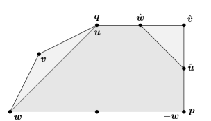
Figure 1: The boundary points of $\mathcal{P}$ given in Definition 9.28. In this example, $\boldsymbol{q}=\boldsymbol{u}$ and $\boldsymbol{p}=-\boldsymbol{w}$, but these equalities need not hold in general.

See Figure 1 for an illustration. Note that $\boldsymbol{p},\hat{\boldsymbol{v}},\boldsymbol{q},\boldsymbol{u},\boldsymbol{w}$ are all vertices of $\mathcal{P}$, and that $\boldsymbol{p}\leq\hat{\boldsymbol{u}}<\hat{\boldsymbol{v}}<\hat{\boldsymbol{w}}\leq\boldsymbol{q}$ since $-\boldsymbol{v}$ is the unique vertex of $\mathcal{P}$ for which $L_{-\boldsymbol{v}}$ separates $\hat{\boldsymbol{v}}$ from all other vertices of $\mathcal{P}$. We adopt the notation of Definition 9.28 in Propositions 9.29 and 9.31 below.

Proposition 9.29

The symmetric difference of $V(\mathcal{P}_{\boldsymbol{v}})$ and $V(\mathcal{P})$ satisfies

$$\left\{\pm\boldsymbol{v},\pm\hat{\boldsymbol{v}}\right\}\subseteq V(\mathcal{P}_{\boldsymbol{v}})\triangle V(\mathcal{P})\subseteq\left\{\pm\boldsymbol{v},\pm\hat{\boldsymbol{v}},\pm\boldsymbol{u},\pm\hat{\boldsymbol{u}},\pm\boldsymbol{w},\pm\hat{\boldsymbol{w}}\right\}.$$

Proof 9.30

Proof. The boundary of $S_{\boldsymbol{v}}$ is $\pm L_{\boldsymbol{v}}$, so any vertex of $\mathcal{P}_{\boldsymbol{v}}$ that is not contained in $\mathcal{P}$ must lie in

$$(\mathcal{P}\cup\left\{\pm\boldsymbol{v}\right\})\cap(\pm L_{\boldsymbol{v}})=\mathcal{P}\cap(\pm L_{\boldsymbol{v}})=\pm\left[\hat{\boldsymbol{u}},\hat{\boldsymbol{w}}\right]$$

by Proposition 9.24. Hence

$$\left\{\pm\boldsymbol{v}\right\}\subseteq V(\mathcal{P}_{\boldsymbol{v}})\backslash V(\mathcal{P})\subseteq\left\{\pm\boldsymbol{v},\pm\hat{\boldsymbol{u}},\pm\hat{\boldsymbol{w}}\right\}.$$

We show

$$\left\{\pm\hat{\boldsymbol{v}}\right\}\subseteq V(\mathcal{P})\backslash V(\mathcal{P}_{\boldsymbol{v}})\subseteq\left\{\pm\hat{\boldsymbol{v}},\pm\boldsymbol{u},\pm\boldsymbol{w}\right\}.$$

By assumption, $\boldsymbol{v}\in H_{\hat{\boldsymbol{v}}}^{\mathrm{c}}$ and therefore $-\hat{\boldsymbol{v}}\in H_{\boldsymbol{v}}^{\mathrm{c}}$ which shows $\hat{\boldsymbol{v}}\in V(\mathcal{P})\backslash V(\mathcal{P}_{\boldsymbol{v}})$. Now, let $\boldsymbol{b}\in V(\mathcal{P})\backslash V(\mathcal{P}_{\boldsymbol{v}})$ distinct from $\pm\hat{\boldsymbol{v}}$. Since $\pm\hat{\boldsymbol{u}},\pm\hat{\boldsymbol{w}}\in V(\mathcal{P}_{\boldsymbol{v}})$, $\boldsymbol{b}$ must be a vertex of $\mathrm{conv}(\mathcal{P}\cup\left\{\pm\boldsymbol{v}\right\})$ by Proposition 9.24. Let $\boldsymbol{r},\boldsymbol{s}$ be the vertices of $\mathcal{P}$ such that $\boldsymbol{b}\in L_{\boldsymbol{r}}\cap L_{\boldsymbol{s}}$. If $\boldsymbol{v}\in S_{\boldsymbol{r}}\cap S_{\boldsymbol{s}}$ then $\boldsymbol{b}$ would be a vertex of $S_{\boldsymbol{r}}\cap S_{\boldsymbol{s}}$ which is a parallelogram containing $\mathrm{conv}(\mathcal{P}\cup\left\{\pm\boldsymbol{v}\right\})$, and hence $\boldsymbol{b}$ would be a vertex of $\mathrm{conv}(\mathcal{P}\cup\left\{\pm\boldsymbol{v}\right\})$, a contradiction. So either $\boldsymbol{v}\notin S_{\boldsymbol{r}}$ or $\boldsymbol{v}\notin S_{\boldsymbol{s}}$. It follows that either $\boldsymbol{r}=\pm\hat{\boldsymbol{v}}$ or $\boldsymbol{s}=\pm\hat{\boldsymbol{v}}$. Therefore, $\boldsymbol{b}\in\mathcal{P}\cap(\pm L_{\hat{\boldsymbol{v}}})=\pm\left[\boldsymbol{u},\boldsymbol{w}\right]$, so $\boldsymbol{b}\in\left\{\pm\boldsymbol{u},\pm\boldsymbol{w}\right\}$.

Proposition 9.31

Suppose it is not the case that both $\left|V(\mathcal{P})\right|=6$ and $\boldsymbol{v}\in L_{\boldsymbol{u}}\cap L_{-\boldsymbol{w}}$. Then the symmetric difference of $V(\mathcal{P}_{\boldsymbol{v}})$ and $V(\mathcal{P})$ has size 8 and is given by

$$V(\mathcal{P}_{\boldsymbol{v}})\triangle V(\mathcal{P})=\left\{\pm\boldsymbol{v},\pm\hat{\boldsymbol{v}},\pm\tilde{\boldsymbol{u}},\pm\tilde{\boldsymbol{w}}\right\}$$

for some $\tilde{\boldsymbol{u}}\in\left\{\pm\boldsymbol{u},\pm\hat{\boldsymbol{u}}\right\}$ and some $\tilde{\boldsymbol{w}}\in\left\{\pm\boldsymbol{w},\pm\hat{\boldsymbol{w}}\right\}$.

Proof 9.32

Proof. We have $\boldsymbol{u},\boldsymbol{w}\in V(\mathcal{P})$ and $\hat{\boldsymbol{u}},\hat{\boldsymbol{w}}\in V(\mathcal{P}_{\boldsymbol{v}})$. Applying Proposition 9.29, we would like to show that $\hat{\boldsymbol{u}}\in V(\mathcal{P})$ if and only if $\boldsymbol{u}\notin V(\mathcal{P}_{\boldsymbol{v}})$, and similarly $\hat{\boldsymbol{w}}\in V(\mathcal{P})$ if and only if $\boldsymbol{w}\notin V(\mathcal{P}_{\boldsymbol{v}})$. We sketch the argument of the former claim; the latter claim is analogous.

Suppose $\hat{\boldsymbol{u}}\in V(\mathcal{P})$. Then $\hat{\boldsymbol{u}}=\boldsymbol{p}$. This implies $\boldsymbol{u},\boldsymbol{v}\in L_{\boldsymbol{p}}$. Suppose for a contradiction $\boldsymbol{u}\in V(\mathcal{P}_{\boldsymbol{v}})$. Then $\mathcal{P}_{\boldsymbol{v}}\cap L_{\boldsymbol{p}}=\left[\boldsymbol{u},\boldsymbol{v}\right]$, and since $\boldsymbol{u}\in\mathcal{P}\cap L_{\hat{\boldsymbol{v}}}$ but $L_{\hat{\boldsymbol{v}}}$ separates $\boldsymbol{v}$ from $\mathcal{P}$, we get $\mathcal{P}\cap\left[\boldsymbol{u},\boldsymbol{v}\right]=\left\{\boldsymbol{u}\right\}$. Meanwhile $\mathcal{P}\cap L_{\boldsymbol{p}}=\left[\boldsymbol{u}^{\prime},\boldsymbol{u}\right]$ for some vertex $\boldsymbol{u}^{\prime}$ of $\mathcal{P}$, which shows $\boldsymbol{u}\in(\boldsymbol{u}^{\prime},\boldsymbol{v})$. It follows that $\boldsymbol{u}^{\prime}$ is a vertex of $\mathcal{P}$ outside of $S_{\boldsymbol{v}}$, since otherwise $\boldsymbol{u}$ would not be a vertex of $\mathcal{P}_{\boldsymbol{v}}$. Since $-\boldsymbol{w}<\hat{\boldsymbol{v}}\leq\boldsymbol{u}^{\prime}<\boldsymbol{u}<\boldsymbol{w}$ we have $\boldsymbol{u}^{\prime}=\hat{\boldsymbol{v}}$. Hence $\boldsymbol{u}=\boldsymbol{q}$. It follows that $\hat{\boldsymbol{v}}<\boldsymbol{u}<\boldsymbol{w}$ are consecutive vertices of $\mathcal{P}$ in the counterclockwise ordering. Since $\boldsymbol{u},\boldsymbol{w}\in L_{\hat{\boldsymbol{v}}}$, we get by Proposition 9.12 that $\left|V(\mathcal{P})\right|=6$. We have $\boldsymbol{v}\in L_{-\boldsymbol{w}}$ since there are only six vertices and hence $-\boldsymbol{w}=\boldsymbol{p}=\hat{\boldsymbol{u}}$. Since $\mathcal{P}_{\boldsymbol{v}}\cap L_{\boldsymbol{p}}=\left[\boldsymbol{u},\boldsymbol{v}\right]$ and since $\boldsymbol{u}\in(\boldsymbol{u}^{\prime},\boldsymbol{v})$, we have $\mathcal{P}_{\boldsymbol{v}}\cap\left[\boldsymbol{u}^{\prime},\boldsymbol{u}\right]=\left\{\boldsymbol{u}\right\}$. Since $\hat{\boldsymbol{w}}$ is a vertex of $\mathcal{P}_{\boldsymbol{v}}$ for which $\hat{\boldsymbol{w}}\in\left[\hat{\boldsymbol{v}},\boldsymbol{q}\right]=\left[\boldsymbol{u}^{\prime},\boldsymbol{u}\right]$, we get $\boldsymbol{u}=\hat{\boldsymbol{w}}$ and therefore $\boldsymbol{v}\in L_{\boldsymbol{u}}$. Thus $\boldsymbol{v}\in L_{\boldsymbol{u}}\cap L_{-\boldsymbol{w}}$. This contradicts the given hypotheses of the proposition. We conclude $\boldsymbol{u}\notin V(\mathcal{P}_{\boldsymbol{v}})$.

Now suppose $\hat{\boldsymbol{u}}\notin V(\mathcal{P})$. Since $L_{\hat{\boldsymbol{v}}}$ separates $\boldsymbol{v}$ from all other vertices of $\mathcal{P}$, we have that $L_{-\boldsymbol{v}}$ separates $\hat{\boldsymbol{v}}$ from all other vertices of $\mathcal{P}$. Therefore, since $\mathcal{P}\cap L_{-\boldsymbol{v}}=\left[\hat{\boldsymbol{u}},\hat{\boldsymbol{w}}\right]$, we have $\hat{\boldsymbol{u}}$ and $\hat{\boldsymbol{w}}$ both lie in edges incident to $\hat{\boldsymbol{v}}$. Since $\boldsymbol{p}\leq\hat{\boldsymbol{u}}<\hat{\boldsymbol{v}}$ we have in particular that $\hat{\boldsymbol{u}}$ lies in the edge $\left[\boldsymbol{p},\hat{\boldsymbol{v}}\right]$ of $\mathcal{P}$. But this edge is given by the intersection $\mathcal{P}\cap L_{-\boldsymbol{u}}$, which implies $\hat{\boldsymbol{u}}\in L_{-\boldsymbol{u}}$, and therefore $\boldsymbol{u}\in L_{\hat{\boldsymbol{u}}}$. We also have $\boldsymbol{u}\in L_{\boldsymbol{p}}$, and also $\boldsymbol{u}\in\mathcal{P}_{\boldsymbol{v}}$ since $\boldsymbol{u}\in S_{\boldsymbol{v}}$. Now $\boldsymbol{p}\in V(\mathcal{P})$, and by assumption, $\hat{\boldsymbol{u}}\notin V(\mathcal{P})$, which implies $\hat{\boldsymbol{u}}\neq\boldsymbol{p}$. Both $\hat{\boldsymbol{u}},\boldsymbol{p}$ are vertices of $\mathcal{P}_{\boldsymbol{v}}$, the latter since $\boldsymbol{p}\neq\hat{\boldsymbol{v}}$. Therefore, since $\boldsymbol{u}\in\mathcal{P}_{\boldsymbol{v}}$ is contained in the intersection of the two edges $\mathcal{P}_{\boldsymbol{v}}\cap L_{\boldsymbol{p}}$ and $\mathcal{P}_{\boldsymbol{v}}\cap L_{\hat{\boldsymbol{u}}}$, we conclude $\boldsymbol{u}\in V(\mathcal{P}_{\boldsymbol{v}})$.

Proposition 9.33

Suppose $\tau\mathcal{Q}=\mathcal{Q}^{\circ}$ is a polygon such that $\left|V(\mathcal{Q})\right|>6$, and let $\boldsymbol{v}\in V(\mathcal{Q})$. Then there exists a polygon $\mathcal{P}$ such that $\tau\mathcal{P}=\mathcal{P}^{\circ}$, $\boldsymbol{v}$ lies in the interior of $\mathrm{stell}(\mathcal{P})\backslash\mathcal{P}$, and $\mathcal{Q}=\mathcal{P}_{\boldsymbol{v}}$.

Proof 9.34

Proof. Let $\boldsymbol{u},\boldsymbol{w}$ be the vertices of $\mathcal{Q}$ adjacent to $\boldsymbol{v}$, so that $\boldsymbol{u}<\boldsymbol{v}<\boldsymbol{w}$ in the counterclockwise order. The triangle bounded by $L_{-\boldsymbol{u}},L_{-\boldsymbol{v}},L_{-\boldsymbol{w}}$ is the closure of a component of $\mathrm{stell}(\mathcal{Q})\backslash\mathcal{Q}$ by Proposition 9.22. Let $\hat{\boldsymbol{v}}$ be the unique point of $L_{-\boldsymbol{u}}\cap L_{-\boldsymbol{w}}$, which is the unique vertex of this triangle not in $\mathcal{Q}$. Let $\hat{\boldsymbol{u}}<\hat{\boldsymbol{w}}\in V(\mathcal{Q})$ be the other two vertices of this triangle, so that $\mathcal{Q}\cap L_{-\boldsymbol{v}}=\left[\hat{\boldsymbol{u}},\hat{\boldsymbol{w}}\right]$, and let $\mathcal{P}=\mathcal{Q}_{\hat{\boldsymbol{v}}}$. We have

$$\left[\boldsymbol{u},\boldsymbol{w}\right]=\mathcal{Q}\cap L_{\hat{\boldsymbol{v}}}=\mathcal{P}\cap L_{\hat{\boldsymbol{v}}}$$ (17)

where the second equality holds by Proposition 9.24. Since $\tau\mathcal{P}=\mathcal{P}^{\circ}$ by Proposition 9.26, we have $\boldsymbol{u},\boldsymbol{w}$ are vertices of both $\mathcal{P}$ and $\mathcal{Q}$. Since $\left|V(\mathcal{Q})\right|>6$, we therefore apply Proposition 9.31 with respect to the pair $\left(\mathcal{Q},\hat{\boldsymbol{v}}\right)$, which corresponds to the Definition 9.28 sequence

$$-\hat{\boldsymbol{w}}\leq-\boldsymbol{u}\leq-\boldsymbol{u}<-\boldsymbol{v}<-\boldsymbol{w}\leq-\boldsymbol{w}\leq\hat{\boldsymbol{u}}<\hat{\boldsymbol{w}}$$

of boundary points of $\mathcal{Q}$, to get

$$V(\mathcal{P})\triangle V(\mathcal{Q})=\left\{\pm\boldsymbol{v},\pm\hat{\boldsymbol{v}},\pm\hat{\boldsymbol{u}},\pm\hat{\boldsymbol{w}}\right\}.$$ (18)

Let $\boldsymbol{p}<\hat{\boldsymbol{v}}<\boldsymbol{q}$ be consecutive vertices of $\mathcal{P}$ in the counterclockwise ordering. Then $L_{\boldsymbol{p}},L_{\hat{\boldsymbol{v}}},L_{\boldsymbol{q}}$ bound the closure of a component of $\mathrm{stell}(\mathcal{P})\backslash\mathcal{P}$ by Proposition 9.22. We show $\boldsymbol{v}$ lies in the interior of this component. The fact that $\hat{\boldsymbol{v}}\notin H_{-\boldsymbol{v}}$ implies $\boldsymbol{v}\notin H_{\hat{\boldsymbol{v}}}$. To see $\boldsymbol{v}\in H_{\boldsymbol{p}}\cap H_{\boldsymbol{q}}$ it suffices to show $\boldsymbol{p},\boldsymbol{q}$ are vertices of $\mathcal{Q}$, which is equivalent to saying $\boldsymbol{p},\boldsymbol{q}\notin V(\mathcal{P})\triangle V(\mathcal{Q})$. Since $\boldsymbol{v}\notin\mathcal{P}$ and $\boldsymbol{p}<\hat{\boldsymbol{v}}<\boldsymbol{q}$ we have $\boldsymbol{p},\boldsymbol{q}\notin\left\{\pm\boldsymbol{v},\pm\hat{\boldsymbol{v}}\right\}$. Since $\hat{\boldsymbol{u}},\hat{\boldsymbol{w}}$ are vertices of $\mathcal{Q}$, by (18) they are not vertices of $\mathcal{P}$, and hence $\boldsymbol{p},\boldsymbol{q}\notin\left\{\pm\hat{\boldsymbol{u}},\pm\hat{\boldsymbol{w}}\right\}$. We also have $\boldsymbol{v}\notin L_{\boldsymbol{p}}$ and $\boldsymbol{v}\notin L_{\boldsymbol{q}}$, since otherwise we would have $\boldsymbol{v}\in\mathcal{Q}\cap L_{\hat{\boldsymbol{u}}}\cap L_{\hat{\boldsymbol{w}}}\cap L_{\boldsymbol{p}}$ or $\boldsymbol{v}\in\mathcal{Q}\cap L_{\hat{\boldsymbol{u}}}\cap L_{\hat{\boldsymbol{w}}}\cap L_{\boldsymbol{q}}$. As $\hat{\boldsymbol{u}},\hat{\boldsymbol{w}},\boldsymbol{p},\boldsymbol{q}\in V(\mathcal{P})$ are pairwise distinct, either case would imply that $\boldsymbol{v}$ lies in the intersection of three edges of $\mathcal{Q}$, a contradiction.

The final step is to show $\mathcal{P}_{\boldsymbol{v}}=\mathcal{Q}$. We begin by showing $\mathcal{P}\cap L_{\hat{\boldsymbol{v}}}=\left[\boldsymbol{u},\boldsymbol{w}\right]$ and $\mathcal{P}\cap L_{-\boldsymbol{v}}=\left[\hat{\boldsymbol{u}},\hat{\boldsymbol{w}}\right]$. The former equality holds by (17). We establish the latter equality. Observe that $\hat{\boldsymbol{u}},\hat{\boldsymbol{w}}$ both lie on the boundary of $\mathcal{P}$. Indeed, $\hat{\boldsymbol{u}},\hat{\boldsymbol{w}}$ are vertices of $\mathcal{Q}$ distinct from $\boldsymbol{v}$, which means $\hat{\boldsymbol{u}},\hat{\boldsymbol{w}}\in S_{\hat{\boldsymbol{v}}}$ and therefore $\hat{\boldsymbol{u}},\hat{\boldsymbol{w}}\in\mathcal{P}$. Since $\boldsymbol{u},\boldsymbol{w}\in V(\mathcal{P})$, we have $\mathcal{P}\cap L_{-\boldsymbol{u}}$ and $\mathcal{P}\cap L_{-\boldsymbol{w}}$ are two edges of $\mathcal{P}$ which contain $\hat{\boldsymbol{u}}$ and $\hat{\boldsymbol{w}}$, respectively. The fact that $\hat{\boldsymbol{u}},\hat{\boldsymbol{w}}\in L_{-\boldsymbol{v}}$ concludes the claim $\mathcal{P}\cap L_{-\boldsymbol{v}}=\left[\hat{\boldsymbol{u}},\hat{\boldsymbol{w}}\right]$.

Note that $\boldsymbol{v}\notin L_{\boldsymbol{u}}\cap L_{-\boldsymbol{w}}$. This is equivalent to the statement $\mathcal{Q}\cap L_{-\boldsymbol{v}}\neq\left[\boldsymbol{u},-\boldsymbol{w}\right]$, which is true because we already know $\mathcal{Q}\cap L_{-\boldsymbol{v}}=\left[\hat{\boldsymbol{u}},\hat{\boldsymbol{w}}\right]$ and that $\hat{\boldsymbol{u}},\hat{\boldsymbol{w}}\notin V(\mathcal{P})$ by (18). We have

$$\left[\hat{\boldsymbol{u}},\hat{\boldsymbol{w}}\right]=\mathcal{P}\cap L_{-\boldsymbol{v}}=\mathcal{P}_{\boldsymbol{v}}\cap L_{-\boldsymbol{v}}$$

where again the second equality holds by Proposition 9.24, and since $-\boldsymbol{v}\in V(\mathcal{P}_{\boldsymbol{v}})$ and $\tau\mathcal{P}_{\boldsymbol{v}}=(\mathcal{P}_{\boldsymbol{v}})^{\circ}$ we get as before $\hat{\boldsymbol{u}},\hat{\boldsymbol{w}}\in V(\mathcal{P}_{\boldsymbol{v}})$. We again apply Proposition 9.31, this time in terms of the pair $\left(\mathcal{P},\boldsymbol{v}\right)$. We get

$$V(\mathcal{P}_{\boldsymbol{v}})\triangle V(\mathcal{P})=\left\{\pm\boldsymbol{v},\pm\hat{\boldsymbol{v}},\pm\hat{\boldsymbol{u}},\pm\hat{\boldsymbol{w}}\right\}.$$

Thus the vertex sets of $\mathcal{P}_{\boldsymbol{v}}$ and $\mathcal{Q}$ agree.

Definition 9.35

Let $\mathcal{Q}=\mathcal{P}_{\boldsymbol{v}}$ as in Proposition 9.33, and assume the notation of Definition 9.28 with respect to the pair $(\mathcal{P},\boldsymbol{v})$. Let $\boldsymbol{v}_{0}=\boldsymbol{u}$ and let $\boldsymbol{v}_{1}\in L_{\hat{\boldsymbol{u}}}\cap L_{\boldsymbol{q}}$. For $\lambda\in\left[0,1\right]$, let $\boldsymbol{v}_{\lambda}=(1-\lambda)\boldsymbol{v}_{0}+\lambda\boldsymbol{v}_{1}$. Let $\hat{\boldsymbol{w}}_{\lambda}$ denote the unique point in $L_{-\boldsymbol{v}_{\lambda}}\cap L_{-\boldsymbol{w}}$. Finally, let

$$\mathcal{P}_{\lambda}:=\mathcal{P}_{\boldsymbol{v}_{\lambda}}.$$

Note that this definition is well-defined since $\boldsymbol{v}_{\lambda}\in\mathrm{stell}(\mathcal{P})$. By Proposition 9.26, we have $\tau\mathcal{P}_{\lambda}=(\mathcal{P}_{\lambda})^{\circ}$. Note that $\mathcal{P}=\mathcal{P}_{0}$ and that $\boldsymbol{v}=\boldsymbol{v}_{\lambda}$ for some $\lambda\in(0,1)$ since $\boldsymbol{v}\in L_{\hat{\boldsymbol{u}}}\cap L_{\hat{\boldsymbol{w}}}$ and $L_{\hat{\boldsymbol{u}}}$ intersects the boundary of the component of $\mathrm{stell}(\mathcal{P})\backslash\mathcal{P}$ containing $\boldsymbol{v}$ at $\boldsymbol{v}_{0}$ and $\boldsymbol{v}_{1}$. Hence, we have $\mathcal{Q}=\mathcal{P}_{\boldsymbol{v}}=\mathcal{P}_{\boldsymbol{v}_{\lambda}}=\mathcal{P}_{\lambda}$. See Figure 2 for an illustration of Definition 9.35.

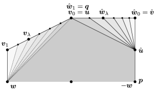
Figure 2: The polytopes $\mathcal{P}_{\lambda}$ for $\lambda\in\left\{0,\tfrac{1}{6},\frac{2}{6},\tfrac{3}{6},\frac{4}{6},\frac{5}{6},1\right\}$.

Proposition 9.36

Let $\lambda\in\left[0,1\right]$, and write $\hat{\boldsymbol{w}}_{\lambda}=(1-\mu)\hat{\boldsymbol{v}}+\mu\boldsymbol{q}$. Then

$$\mu=\frac{\lambda a}{\lambda a+(1-\lambda)b},$$

where $a:=\det(\hat{\boldsymbol{v}},\boldsymbol{v}_{1}-\boldsymbol{u})$ and $b:=\det(\boldsymbol{u},\boldsymbol{q}-\hat{\boldsymbol{v}})$.

Figure 2 demonstrates the nonlinear dependence of $\mu$ on $\lambda$.

Proof 9.37

Proof. Since $\hat{\boldsymbol{w}}_{\lambda}\in L_{-\boldsymbol{v}_{\lambda}}$ we have

$$1 =-(\tau\boldsymbol{v}_{\lambda})^{\top}\hat{\boldsymbol{w}}_{\lambda}$$

$$=\det((1-\mu)\hat{\boldsymbol{v}}+\mu\boldsymbol{q},(1-\lambda)\boldsymbol{u}+\lambda\boldsymbol{v}_{1})$$

$$=\det(\hat{\boldsymbol{v}}+\mu(\boldsymbol{q}-\hat{\boldsymbol{v}}),\boldsymbol{u}+\lambda(\boldsymbol{v}_{1}-\boldsymbol{u}))$$

$$=1+\lambda a-\mu b+\lambda\mu\det(\boldsymbol{q}-\hat{\boldsymbol{v}},\boldsymbol{v}_{1}-\boldsymbol{u}).$$

Since $\boldsymbol{u}\in L_{\hat{\boldsymbol{v}}}$ and $\boldsymbol{v}_{1}\in L_{\boldsymbol{q}}$ we have $\det(\boldsymbol{q},\boldsymbol{v}_{1})=1=\det(\hat{\boldsymbol{v}},\boldsymbol{u})$. Hence

$$\det(\boldsymbol{q}-\hat{\boldsymbol{v}},\boldsymbol{v}_{1}-\boldsymbol{u}) =\det(\boldsymbol{q},\boldsymbol{v}_{1})-\det(\boldsymbol{q},\boldsymbol{u})-a$$ (19)

$$=\det(\hat{\boldsymbol{v}},\boldsymbol{u})-\det(\boldsymbol{q},\boldsymbol{u})-a$$

$$=b-a,$$

and therefore we get

$$1=1+\lambda a-\mu b+\lambda\mu(b-a).$$

Solving for $\mu$ yields the desired equality.

Proposition 9.38

For $\lambda\in\left[0,1\right]$, we have

$$\mathrm{vol}(\mathcal{P}_{\lambda}) \geq\min\{\mathrm{vol}(\mathcal{P}_{0}),\mathrm{vol}(\mathcal{P}_{1})\}.$$

Proof 9.39

Proof. Observe that

$$\mathrm{vol}(\mathcal{P}_{0}\backslash\mathcal{P}_{\lambda}) =\left|\det(\hat{\boldsymbol{v}}-\hat{\boldsymbol{u}},\hat{\boldsymbol{w}}_{\lambda}-\hat{\boldsymbol{u}})\right|=\mu\left|\det(\hat{\boldsymbol{v}}-\hat{\boldsymbol{u}},\boldsymbol{q}-\hat{\boldsymbol{u}})\right|$$

$$\mathrm{vol}(\mathcal{P}_{\lambda}\backslash\mathcal{P}_{0}) =\left|\det(\boldsymbol{u}-\boldsymbol{w},\boldsymbol{v}_{\lambda}-\boldsymbol{w})\right|=\lambda\left|\det(\boldsymbol{u}-\boldsymbol{w},\boldsymbol{v}_{1}-\boldsymbol{w})\right|.$$

We have

$$\mathrm{vol}(\mathcal{P}_{\lambda})=\mathrm{vol}(\mathcal{P}_{0})+\mathrm{vol}(\mathcal{P}_{\lambda}\backslash\mathcal{P}_{0})-\mathrm{vol}(\mathcal{P}_{0}\backslash\mathcal{P}_{\lambda}),$$

and so

$$\frac{\mathrm{d}^{2}\mathrm{vol}(\mathcal{P}_{\lambda})}{\mathrm{d}\lambda^{2}}=-\left|\det(\hat{\boldsymbol{v}}-\hat{\boldsymbol{u}},\boldsymbol{q}-\hat{\boldsymbol{u}})\right|\cdot\frac{\mathrm{d}^{2}\mu}{\mathrm{d}\lambda^{2}}.$$

Hence we are done if we can show $\mu=\mu(\lambda)$ is convex on $\lambda\in\left[0,1\right]$, as this would imply that the minimum of $\mathrm{vol}(\mathcal{P}_{\lambda})$ is attained at either $\lambda=0$ or $\lambda=1$. By Proposition 9.36, we have

$$\frac{\mathrm{d}^{2}\mu}{\mathrm{d}\lambda^{2}}=\frac{2ab(b-a)}{(\lambda a+(1-\lambda)b)^{3}}.$$

It therefore remains to show $b\geq a>0$. Since $\boldsymbol{v}_{1}$ is separated from $\mathcal{P}$ by $L_{\hat{\boldsymbol{v}}}$ we have $\det(\hat{\boldsymbol{v}},\boldsymbol{v}_{1})>1$. Since $\det(\hat{\boldsymbol{v}},\boldsymbol{u})=1$ we get $a>0$. To see that $b-a>0$, we use the representation of (19) to write $b-a=\det(\boldsymbol{q}-\hat{\boldsymbol{v}},\boldsymbol{v}_{1}-\boldsymbol{u})$. We have $\boldsymbol{q},\hat{\boldsymbol{v}}\in L_{-\boldsymbol{w}}$, which implies $\boldsymbol{q}-\hat{\boldsymbol{v}}$ is a scalar multiple of $\boldsymbol{w}$. Since $-\boldsymbol{w}<\hat{\boldsymbol{v}}<\boldsymbol{q}<\boldsymbol{w}$ along the boundary of $\mathcal{P}$ in the counterclockwise order, we have that $\boldsymbol{q}-\hat{\boldsymbol{v}}$ is a positive multiple of $\boldsymbol{w}$. In a similar manner, we have $\boldsymbol{v}_{1},\boldsymbol{u}\in L_{\hat{\boldsymbol{u}}}$ which implies $\boldsymbol{v}_{1}-\boldsymbol{u}$ is a scalar multiple of $\hat{\boldsymbol{u}}$. Since $-\boldsymbol{w}<\hat{\boldsymbol{u}}<\boldsymbol{u}<\boldsymbol{v}_{1}<\boldsymbol{w}<-\hat{\boldsymbol{u}}$ along the boundary of $\mathcal{P}_{1}$ in the counterclockwise order, $\boldsymbol{v}_{1}-\boldsymbol{u}$ is a negative multiple of $\hat{\boldsymbol{u}}$. We conclude that $b-a$ has the same sign as $\det(\boldsymbol{w},-\hat{\boldsymbol{u}})$. Since $-\boldsymbol{w}<\hat{\boldsymbol{u}}<\boldsymbol{w}$ in the counterclockwise order of $\mathcal{P}$, this determinant is positive.

Proposition 9.40

For $\lambda\in(0,1)$, we have

$$\left|V(\mathcal{P}_{\lambda})\right| >\max\{\left|V(\mathcal{P}_{0})\right|,\left|V(\mathcal{P}_{1})\right|\}.$$

Proof 9.41

Proof. We have $\hat{\boldsymbol{u}}\in(\boldsymbol{p},\hat{\boldsymbol{v}})$ and therefore $\hat{\boldsymbol{u}}\notin V(\mathcal{P})$. Since $\lambda\in(0,1)$, and $\hat{\boldsymbol{w}}_{\lambda}\in(\hat{\boldsymbol{v}},\boldsymbol{q})$, we also have $\hat{\boldsymbol{w}}_{\lambda}\notin V(\mathcal{P})$. Therefore, by Proposition 9.31, we have

$$V(\mathcal{P}_{\lambda})=(V(\mathcal{P})\backslash\left\{\pm\hat{\boldsymbol{v}}\right\})\cup\left\{\pm\boldsymbol{v}_{\lambda},\pm\hat{\boldsymbol{u}},\pm\hat{\boldsymbol{w}}_{\lambda}\right\}.$$

Now $L_{-\boldsymbol{v}_{1}}\cap\mathcal{P}=\left[\hat{\boldsymbol{u}},\boldsymbol{q}\right]$. We have $\boldsymbol{q}\in V(\mathcal{P})$, and therefore by Proposition 9.31, we have

$$V(\mathcal{P}_{1})=(V(\mathcal{P})\backslash\left\{\pm\hat{\boldsymbol{v}},\pm\boldsymbol{q}\right\})\cup\left\{\pm\boldsymbol{v}_{1},\pm\hat{\boldsymbol{u}}\right\}.$$

Since $\boldsymbol{v}_{0}=\boldsymbol{u}$, we have $\mathcal{P}_{0}=\mathcal{P}$, and therefore we conclude

$$\left|V(\mathcal{P}_{\lambda})\right|>\left|V(\mathcal{P}_{0})\right|=\left|V(\mathcal{P}_{1})\right|.$$

Recall the statement of Lemma 4.1: if $\mathcal{Q}$ is a polygon satisfying $\tau\mathcal{Q}\subseteq\mathcal{Q}^{\circ}$ then $\mathrm{vol}(\mathcal{Q}^{\circ})\geq 3$.

Proof 9.42

Proof of Lemma 4.1. Suppose $\mathcal{Q}$ is a polygon satisfying $\tau\mathcal{Q}\subseteq\mathcal{Q}^{\circ}$. By Proposition 9.19, we may assume without loss of generality that $\tau\mathcal{Q}=\mathcal{Q}^{\circ}$. Then $\left|V(\mathcal{Q})\right|\geq 6$ by Proposition 9.10. If $\left|V(\mathcal{Q})\right|=6$ then $\mathrm{vol}(\mathcal{Q})=3$ by Proposition 9.14. Otherwise, $\left|V(\mathcal{Q})\right|>6$. By Proposition 9.33, there exists $\boldsymbol{v}\in V(\mathcal{Q})$ such that $\mathcal{Q}=\mathcal{P}_{\boldsymbol{v}}$ for some $\boldsymbol{v}$ in the interior of $\mathrm{stell}(\mathcal{P})\backslash\mathcal{P}$. For $\lambda\in\left[0,1\right]$, let $\mathcal{P}_{\lambda}$ be the polytope of Definition 9.35, in terms of the pair $(\mathcal{P},\boldsymbol{v})$, so that in particular there exists some $\lambda\in(0,1)$ such that $\mathcal{Q}=\mathcal{P}_{\lambda}$. By Proposition 9.38, there exists $i\in\left\{0,1\right\}$ for which $\mathrm{vol}(\mathcal{Q})\geq\mathrm{vol}(\mathcal{P}_{i})$. By Proposition 9.40, $\left|V(\mathcal{Q})\right|>\left|V(\mathcal{P}_{i})\right|$. By induction on the number of vertices, we have $\mathrm{vol}(\mathcal{P}_{i})\geq 3$, and therefore $\mathrm{vol}(\mathcal{Q}^{\circ})=\mathrm{vol}(\tau\mathcal{Q})=\mathrm{vol}(\mathcal{Q})\geq 3$.

Acknowledgements.

J. Paat was supported by a Natural Sciences and Engineering Research Council of Canada (NSERC) Discovery Grant [RGPIN-2021-02475]. R. Weismantel was supported by the Einstein Foundation Berlin.

References

- Aliev et al. [2021] Aliev I, Celaya M, Henk M, Williams A (2021) Distance-sparsity transference for vertices of corner polyhedra. SIAM Journal on Optimization 31:200–126, URL http://dx.doi.org/10.1137/20M1353228.
- Aliev et al. [2020] Aliev I, Henk M, Oertel T (2020) Distances to lattice points in knapsack polyhedra. Mathematical Programming 182:175–198, URL http://dx.doi.org/10.1007/s10107-019-01392-1.
- Celaya et al. [2022] Celaya M, Kuhlmann S, Paat J, Weismantel R (2022) Improving the Cook et al. proximity bound given integral valued constraints. Integer Programming and Combinatorial Optimization, 84 – 97 (Springer International Publishing), URL http://dx.doi.org/10.1007/978-3-031-06901-7_7.
- Cook et al. [1986] Cook W, Gerards A, Schrijver A, Tardos E (1986) Sensitivity theorems in integer linear programming. Mathematical Programming 34:251–264, URL http://dx.doi.org/10.1007/BF01582230.
- Del Pia and Ma [2021] Del Pia A, Ma M (2021) Proximity in concave integer quadratic programming. Available online: arXiv:2006.01718 .
- Eisenbrand and Weismantel [2020] Eisenbrand F, Weismantel R (2020) Proximity Results and Faster Algorithms for Integer Programming Using the Steinitz Lemma. ACM Transactions on Algorithms 16:1–14, URL http://dx.doi.org/10.1145/3340322.
- Fischetti et al. [2005] Fischetti M, Glover F, Lodi A (2005) The feasibility pump. Mathematical Programming 104:91–104, URL http://dx.doi.org/10.1007/s10107-004-0570-3.
- Florian [1996] Florian A (1996) On the area sum of a convex set and its polar reciprocal. Mathematica Pannonica 171:176.
- Fortier [2020] Fortier JM (2020) Self-nolar Planar Polytopes: When Finding the Polar is Rotating by Pi. Master’s thesis, Concordia University.
- Granot and Skorin-Kapov [1990] Granot F, Skorin-Kapov J (1990) Some proximity and sensitivity results in quadratic integer programming. Mathematical Programming 47:259–268, URL http://dx.doi.org/10.1007/BF01580862.
- Gribanov and Veselov [2016] Gribanov D, Veselov S (2016) On integer programming with bounded determinants. Optimization Letters 10:1169–1177.
- Gruber [2007] Gruber P (2007) Convex and Discrete Geometry (Springer-Verlag Berlin Heidelberg).
- Henk et al. [2022] Henk M, Kuhlmann S, Weismantel R (2022) On lattice width of lattice-free polyhedra and height of Hilbert bases. SIAM Journal on Discrete Mathematics 36(3):1918–1942.
- Hochbaum and Shanthikumar [1990] Hochbaum DS, Shanthikumar JG (1990) Convex separable optimization is not much harder than linear optimization. Journal of the ACM 37:843–862, URL http://dx.doi.org/10.1145/96559.96597.
- Jansen and Rohwedder [2019] Jansen K, Rohwedder L (2019) On Integer Programming and Convolution. 10th Innovations in Theoretical Computer Science, volume 43, 43:1–43:17, URL http://dx.doi.org/10.4230/LIPIcs.ITCS.2019.43.
- Jensen [2021] Jensen A (2021) Self-polar polytopes. Polytopes and Discrete Geometry, Contemporary Mathematics (American Mathematical Society), URL http://dx.doi.org/10.1090/conm/764.
- Jiang and Basu [2022] Jiang H, Basu A (2022) Enumerating integer points in polytopes with bounded subdeterminants. SIAM Journal on Discrete Mathematics 36(1):449–460, URL http://dx.doi.org/10.1137/21M139935X.
- Khinchine [1948] Khinchine A (1948) A quantitative formulation of Kronecker’s theory of approximation. Izv. Acad. Nauk SSSR 12:113 – 122.
- Lee et al. [2020] Lee J, Paat J, Stallknecht I, Xu L (2020) Improving proximity bounds using sparsity. Proceedings of the 2020 International Symposium on Combinatorial Optimization 115–127, URL http://dx.doi.org/10.1007/978-3-030-53262-8_10.
- Lee et al. [2021] Lee J, Paat J, Stallknecht I, Xu L (2021) Polynomial upper bounds on the number of differing columns of -modular integer programs. arXiv:2105.08160 .
- Lenstra [1983] Lenstra H (1983) Integer programming with a fixed number of variables. Mathematics of Operations Research 8(4):538 – 548.
- Mahler [1939] Mahler K (1939) Ein übertragungsprinzip für konvexe Körper (in German). Časopis Pešt. Mat. Fyz. 68:93–102.
- Nägele et al. [2022] Nägele M, Santiago R, Zenklusen R (2022) Congruency-constrained TU problems beyond the bimodular case. In proceedings of SODA 2022 URL http://dx.doi.org/10.1137/1.9781611977073.108.
- Oertel et al. [2020] Oertel T, Paat J, Weismantel R (2020) The distributions of functions related to parametric integer optimization. SIAM Journal on Applied Algebra and Geometry 422–440, URL http://dx.doi.org/10.1137/19M1275954.
- Paat et al. [2020] Paat J, Weismantel R, Weltge S (2020) Distances between optimal solutions of mixed-integer programs. Mathematical Programming 179:455–468, URL http://dx.doi.org/10.1007/s10107-018-1323-z.
- Rudelson [2000] Rudelson M (2000) Distances between nonsymmetric convex bodies and the MM*-estimate. Positivity 4:2:161–178.
- Santos [2012] Santos F (2012) A counterexample to the Hirsch Conjecture. Annals of Mathematics 176:383–412, URL http://dx.doi.org/10.4007/annals.2012.176.1.7.
- Schrijver [1986] Schrijver A (1986) Theory of linear and integer programming (John Wiley & Sons, Inc. New York, NY).
- Sturmfels [1996] Sturmfels B (1996) Gröbner bases and convex polytopes (University Lecture Series, Volume 8, 162 pp.).
- Veselov and Chirkov [2009] Veselov S, Chirkov A (2009) Integer programming with bimodular matrix. Discrete Optimization 6:220–222, URL http://dx.doi.org/10.1016/j.disopt.2008.12.002.
- Werman and Magagnosc [1991] Werman M, Magagnosc D (1991) The relationship between integer and real solutions of constrained convex programming. Mathematical Programming 51:133–135, URL http://dx.doi.org/10.1007/BF01586929.
- Xu and Lee [2019] Xu L, Lee J (2019) On proximity for -regular mixed-integer linear optimization. Proceedings of WCGO 2019, 438–447 (Springer), URL http://dx.doi.org/10.1007/978-3-030-21803-4_44.