Targeted Demand Response: Formulation, LMP Implications, and Fast Algorithms

Abstract

Demand response (DR) is regarded as a solution to the issue of high electricity prices in the wholesale market, as the flexibility of the demand can be harnessed to lower the demand level for price reductions. As an across-the-board DR in a system is impractical due to the enrollment budget for instance, it is necessary to select a small group of nodes for DR implementing. Current studies resort to intuitive yet naive approaches for DR targeting, as price is implicitly associated with demand, though optimality cannot be ensured. In this paper, we derive such a relationship in the security-constrained economic dispatch via the multi-parametric programming theory, based on which the DR targeting problem is rigorously formulated as a mixed-integer quadratic programming problem aiming at reducing the averaged price to a reference level by efficiently reducing targeted nodes’ demand. A solution strategy is proposed to accelerate the computation. Numerical studies demonstrate compared with the benchmarking strategy, the proposed approach can reduce the price to the reference point with less efforts in demand reduction. Besides, we empirically show that the proposed approach is immune to inaccurate system parameters, and can be generalized to variants of DR targeting tasks.

Keywords: Demand response, targeting, electricity price, multi-parametric programming

I Introduction

Demand response (DR) involves the active participation of retail customers in electricity markets, which encourages the adaptability of electricity consumption plans in response to dynamic price or incentives [1]. Due to the potential benefits brought by DR on power grid efficiency and reliability, many efforts have been devoted to elicit flexibility from customers, including the retail price design [2, 3], direct load control [4, 5], and incentive design [6, 7]. And in the U.S., there are already 11.7 million customers enrolled in DR programs in 2020 [8]. With the huge DR capacity, the benefits of DR to power systems management are also becoming evident.

Although customers have great potentials in providing flexibility via well-designed DR programs, it is intractable for them to directly interact with the system operators [9]. Therefore, intermediate entities, such as load-serving entities (LSEs), are required to aggregate DR resources from customers and interact with both operators and customers. Accordingly, the intermediate entities can benefit from such DR programs [10]. Take a LSE as an example, it bears the price risk as a result of the spot price spike in the wholesale market and then resells the electricity to the served customers at a fixed retail rate. Therefore, reducing demands via DR programs during a price spike is beneficial to managing such risk for LSEs. In addition to that, it can lower the risk and extent of forced outages to enhance system-level reliability by offering load reduction.

The economic benefits from DR are also prominent; several grid operators, e.g. NYISO, PJM, ISO-NE, and ERCOT, have taken steps to integrate DR into their wholesale markets [11]. By coordinately shifting nodal demands, DR can lower the wholesale market price by cutting the costs coming from running costly-to-run power plants, and in turn, a reduction in electricity prices. As the decrease in wholesale prices benefits all wholesale market participants, existing studies have investigated the collaboration between LSEs and system operators [6] as well as the corresponding DR mechanisms [12, 13].

However, dispatching universal DR signals throughout all nodes is impractical due to limited DR recruitment budgets or physical constraints. DR targeting, which efficiently selects a subset of candidate locations to participate in DR programs, is essential to the success of DR programs. From the perspective of system operators, not every LSE in a system is allowed to participate in DR programs. Therefore, there is a strong need for implementing DR targeting by determining a set of available and most effective nodes for demand reduction. As system operators are allowed to get access to market and grid information, it is feasible for system operators to perform such mechanisms [14, 15]. And various constraints, such as the cardinality constraint limiting number of DR participants, are needed to be considered. Once selected, the LSEs at the targeted nodes could collaborate with the system operators to reduce their demands as requested.

In this work, we focus on targeting nodes for demand reduction to lower the averaged wholesale market price, which is especially beneficial to both power grid reliability and economics. Previous studies have shown that if nodes are not selected correctly, reducing demand at selected nodes may even lead to higher prices [16, 17]. Moreover, existing price-based control strategies often neglect the physical and operational constraints of the underlying electricity networks when deriving the price [18, 19]. Though reducing demand can act as an “action knob” to lower the electricity price, knowing the relationship between the price and demand under the network constraints is a preliminary step to formulate a targeting problem. Our work is closely related to the intuitive DR targeting method proposed in [20], which sets load targets by taking a reference of historical load data, whose associated averaged nodal prices is below the threshold. Then it determines nodes for DR implementing as well as the nodal demand reduction quantity to let the adjusted load track the selected reference. However, such an approach has not exploited the structure of underlying optimization problems and operational conditions, thereby the resulting DR decisions may not be optimal. We also note that the DR targeting studied in this work is different from DR targeting conducted by LSE, which aims to select an optimal subset of customers to achieve the demand reduction requirement imposed to LSE [21], or to minimize the DR cost [22]. Therefore, it remains an open issue to design efficient DR targeting method in system-level.

Indeed, the nodal electricity price, often referred to as locational marginal price (LMP) in literature, is associated with the dual variables of economic dispatch (ED) problem performed by the operator for market clearing [9]. The nodal LMPs are usually associated with the distinct operating patterns, such as the binding constraints of transmission or generation. And each system operating pattern corresponds to a unique region of nodal demands. Therefore, the relationship between the nodal LMPs and the nodal demands is implicitly reflected in the ED problem. For instance, for an ED problem with the linear objective, the nodal LMPs remain unchanged when demands lie in some specific region. The current literature leverages this property to transform the LMP prediction task to a region classification one for both probabilistic [23] and deterministic [24] forecasts. Yet how to leverage such relationship for finding the optimal DR nodes and DR reductions is still undetermined.

In this paper, we try to answer the following questions:

Are some nodes impacting electricity prices more significantly given demand profiles? How can system operators efficiently select a set of nodal participants to implement DR?

We answer those questions with affirmations by rigorously formulating a DR targeting problem that determines the targeted nodes as locations for implementing DR and the corresponding demand reduction. To achieve these, we use the theoretical relationship between the nodal LMPs and nodal demands to inform the targeting process. Concretely, the nodal LMPs are the results of the optimal dual solutions of a security-constrained economic dispatch (SCED) problem with a quadratic objective, which is performed by the system operators. And we treat the nodal demands as the input parameters of SCED. The relationship between the nodal LMPs and nodal demands, which is denoted as policy in this work, is derived by multi-parametric programming theory [25, 26] and proved to be a piecewise linear function. We show such LMPs policy is making DR targeting practical. With the derived policy, the DR targeting problem is formulated as a mixed-integer quadratic programming (MIQP) problem with multi-objectives, which minimizes the demand reduction cost and the squared error between the averaged LMP and the reference value. Furthermore, to accelerate the solution process, we propose to first judge the feasibility of the relaxed problem of MIQP, which is a quadratic program (QP), before solving the MIQP problem. The case study demonstrates that well-targeted DR schemes can find the nodes which impact the price more significantly than others. Such selected nodes are not the load centers with the highest demand or those with the highest prices, indicating that there is a need to properly select nodes to implement DR actions. More importantly, the averaged electricity price is effectively lowered with a smaller demand reduction, while the proposed algorithm is also much more efficient in terms of computation time.

The main contribution of this paper can be summarized as follows:

1) A rigorous formulation of the DR targeting problem, which sets up the problem in the form of MIQP and determines the targeted nodes and demand reduction optimally.

2) A theoretical derivation of the policy between nodal LMPs and nodal demands, which is further applied to inform the DR targeting process.

3) An acceleration strategy of the solution process, which significantly reduces the computation burden for the original DR targeting problem and makes the proposed framework implementable in a real market environment.

In addition, we also demonstrate proposed framework can be readily applied to a variant of settings, such as DR targeting under inaccurate network models or geographical load shifting. The remaining sections of this paper are organized as follows. Section II introduces the problem setup of SCED, whereas Section III presents the physical framework and formulates the problem. The details of policy derivation and solution strategy are given in Section IV and V, respectively. Results are discussed and evaluated in Section VI, followed by the conclusions.

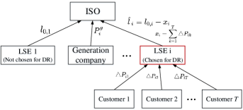
Figure 1: Illustration of the proposed DR targeting framework. When a DR event is triggered, ISO determines the a). targeted nodes and b). the corresponding demand reduction. The LSE connected to the targeted node (plotted in red) reduces the demand as required.

II Preliminaries: Security-Constrained Economic Dispatch

In this paper, we consider a transmission network represented by the graph $\mathcal{G}(\mathcal{N},\mathcal{A})$, where $\mathcal{N}$ is the set of nodes and $\mathcal{A}$ is the set of lines, the SCED problem considers the minimization of the total generation cost $\sum_{i=1}^{|\mathcal{N}|}C_{g}(P_{i}^{g})$, where $P_{i}^{g}$ is the power output of the generator connected to the node $i$, and $C_{g}(\cdot)$ is the generation cost function. Without loss of generality, the quadratic cost is considered in our framework, i.e., $C_{g}(P_{i}^{g})=\frac{1}{2}a_{i}^{g}\cdot(P_{i}^{g})^{2}+b_{i}^{g}\cdot P_{i}^{g}+c_{i}^{g}$. Let $\bm{P}^{g}=[P_{i}^{g}]_{i\in\mathcal{N}}$, $\bm{l}=[l_{i}]_{i\in\mathcal{N}}$ denote the vector formed by the nodal generation power and nodal load. The formulation of SCED problem, which considers each snapshot independently, is as follows:

$$\mathop{\min}_{P_{i}^{g}}\sum_{i=1}^{|\mathcal{N}|}C_{g}(P_{i}^{g})$$ (1a)

$$s.t.\sum_{i=1}^{|\mathcal{N}|}P_{i}^{g}=\sum_{i=1}^{|\mathcal{N}|}l_{i}:\gamma$$ (1b)

$$\quad\ -\bm{f}\leq\bm{H}(\bm{P}^{g}-\bm{l})\leq\bm{f}:\bm{\mu}_{1},\bm{\mu}_{2}$$ (1c)

$$\quad\ \bm{P}^{min}\leq\bm{P}^{g}\leq\bm{P}^{max}:\bm{\psi}_{1},\bm{\psi}_{2};$$ (1d)

where (1b) is the power balance constraint. Given the shift factor matrix $\bm{H}\in\mathbb{R}^{|\mathcal{A}|\times|\mathcal{N}|}$ which maps the nodal power injections to the power flow on lines [27, 28], the transmission constraint is presented in (1c) bounded by the vector of maximum transmission capacity $\bm{f}$. And the generation capacity constraint regarding $\bm{P}^{g}$ is given in (1d), where $\bm{P}^{min}=[P^{min}_{i}]_{i\in\mathcal{N}},\bm{P}^{max}=[P^{max}_{i}]_{i\in\mathcal{N}}$ are the vector regarding the minimum and maximum output power of generators. The dual variables are given behind the colons. Let $\lambda_{i}$ be the LMP at bus $i$. By computing the gradient of the Lagrangian associated with (1) with respect to the demand vector $\bm{l}$, the vector of LMP $\bm{\lambda}=[\lambda_{i}]_{i\in\mathcal{N}}$ can be expressed as [9]:

$$\bm{\lambda}=\gamma^{*}\cdot\bm{1}_{|\mathcal{N}|}-\bm{H}^{T}(\bm{\mu}_{2}^{*}-\bm{\mu}_{1}^{*}),$$ (2)

where $\bm{1}_{|\mathcal{N}|}$ is an all-one column vector with dimension of $|\mathcal{N}|$, and $\gamma^{*},\bm{\mu}_{2}^{*},\bm{\mu}_{1}^{*}$ are the values of optimal dual variables.

Related to the optimal dual solution of (1), the vector of LMP $\bm{\lambda}$ is impacted by the parameters in (1). And the relationship between the optimal dual solution and the parameters of a QP problem, such as the one in (1), is shown to be bijective [26]. Essentially, as the LMP vector $\bm{\lambda}$ is a specific linear transformation of the optimal dual solutions, the relationship between the parameters in (1), such as the vector of load $\bm{l}$, and the LMP vector $\bm{\lambda}$ is also a bijection. We denote such bijection as the policy $\bm{\lambda}=\pi(\bm{l})$ and explicitly describe such price-demand relationship by multi-parametric programming theory in the following discussion.

III Methodological Components

In this section, we first introduce the underlying physical mechanism setup considered in the DR targeting problem in Section III-A. Then, we formulate the DR targeting problem in Section III-B.

III-A The Physical Framework for DR Targeting

The DR targeting framework is sketched in Fig. 1. In real-time energy market operation, the independent system operator (ISO) solves the SCED problem based on predicted nodal demands and derives locational marginal price (LMP, $/MW) at each node. Following the practice in [20], a DR event is triggered once the averaged LMP over all nodes is greater than a threshold (100 $/MW for instance in [20]). To reduce the averaged LMP to a reference value $\lambda^{*}$, it is necessary to dispatch DR signals by reducing the demands at certain nodes.

Firstly, we use a concrete example to show that improper DR targeting can even result in an increase in the averaged LMP. For example, Fig. 2 shows the operation pattern before and after DR of the New England IEEE 39-Bus system, where the red lines and circles display the binding lines and generators. And the node of the DR location is improperly chosen. Concretely, assume the operator reduces the demand of 44.8 MW at node 25. Although the system pattern is not changed after DR, the inappropriate node selection results in the averaged LMP increasing from 105.6303 $/MW to 106.1503 $/MW. Therefore, properly choosing locations for implementing DR is necessary, so as to avoid such adverse effects. And in this work, we assume that ISO shoulders the responsibility of identifying the appropriate set of nodes to implement DR. They also need to determine the corresponding nodal demand reduction as a DR signal. The LSE, which is connected to the DR-targeted node, collects the DR resources from its served customers to fulfill the targeted demand reduction. Meanwhile, the load level remains unchanged for those LSE nodes not chosen for DR.

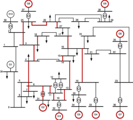
Figure 2: The system pattern before and after DR with improperly targeted node. Binding lines and nodes are shown in red.

III-B The Formulation of DR Targeting Problem

In this subsection, we formulate the DR targeting problem under the policy $\bm{\lambda}=\pi(\bm{l})$. As we focus on the DR targeting problem formulation in this subsection, we assume that the policy is already obtained. Details on obtaining such pricing policy will be discussed in the next Section.

As stated in subsection III-A, in a DR event, one of the major economical objectives is to reduce the nodal prices. And to achieve such goal, ISO needs to determine both the targeted nodes as DR locations and the corresponding demand reduction. Let the binary vector $\bm{v}=[v_{i}]_{i\in\mathcal{N}}$ denote DR/non-DR locations, where $v_{i}=1$ means the node $i$ is chosen as DR location, and $v_{i}=0$ means the node $i$ is not chosen. Let the continuous vector $\bm{x}=[x_{i}]_{i\in\mathcal{N}}$ denote the nodal demand reduction and $\bm{l}_{0}$ denote the nodal load vector before DR. The DR targeting problem seeks to lower the averaged LMP of the system to the reference value $\lambda^{*}$ with the small demand reduction. In this regard, we formulate a multi-objective problem, which is given as

$$\mathop{\min}_{\bm{v},\bm{x}}\quad (\sum_{i\in\mathcal{N}}\lambda_{i}-|\mathcal{N}|\cdot\lambda^{*})^{2}+\bm{w}^{\top}\bm{x}$$ (3a)

$$s.t.\quad \sum_{i\in\mathcal{N}}v_{i}\leq K$$ (3b)

$$\ \bm{0}\leq\bm{x}\leq\bar{\bm{x}}\cdot\bm{v}$$ (3c)

$$\bm{\hat{l}}=\bm{l}_{0}-\bm{x}$$ (3d)

$$\bm{\lambda}=\pi(\bm{\hat{l}}),$$ (3e)

where the objective function (3a) is composed of minimizing the difference between the averaged LMP and the reference value $\lambda^{*}$ along with minimizing the cost of implementing demand reduction. And here we interpret the term $\bm{w}^{\top}\bm{x}$ as the weighted system demand reduction, where the importance of the demand reduction at each node is controlled by a weighting parameter $w_{i}\in\bm{w}$. Constraint (3b) limits that the number of the targeted nodes should be less or equal than a preset integer $K$. Constraint (3c) bounds the demand reduction of the targeted node between 0 and $\bar{x}_{i}$. (3d) gives the new load vector $\bm{\hat{l}}$, which is the original load vector $\bm{l}_{0}$ minus the demand reduction $\bm{x}$. And (3e) maps the new load vector $\bm{\hat{l}}$ to the vector of LMP $\bm{\lambda}$ via the obtained policy $\pi$.

Solving the DR targeting problem (3) is not trivial, since LMP is a product of optimizing the SCED problem, while finding the optimal load reduction deals with the LMP, the binary variables $\bm{v}$ and load reduction $\bm{x}$ simultaneously. In the following sections, we will illustrate obtaining the policy $\pi$ in (3e) is a key but challenging step, and we will detail the solution process for $\pi(\cdot)$ and how it helps find DR targets.

IV Policy Derivation via Multi-parametric Quadratic Programming Theory

In this section, we derive the policy between the vector of LMP and the load vector via multi-parametric quadratic programming theory. An illustrative example is presented in Section IV-A, to intuitively present the policy in one-dimensional space. And the policy derivation algorithm for SCED problem is given in Section IV-B.

IV-A An Illustrative Example

An one-bus numerical example is presented to motivate finding the policy between the LMP and the load, and such analysis can be generalized to any large-scale networks. Consider a simple one-bus system with two generators serving the load $l$. And the generation cost of $C_{g}(P_{1}^{g})$ is cheaper than that of $C_{g}(P_{2}^{g})$ under the same generation level. The SCED problem becomes

$$\mathop{\min}_{P_{i}^{g}}\sum_{i=1}^{2}C_{g}(P_{i}^{g})$$ (4a)

$$s.t.\sum_{i=1}^{2}P_{i}^{g}=l$$ (4b)

$$\quad\ 0\leq P_{i}^{g}\leq P^{max}_{i},\forall i\in\{1,2\}.$$ (4c)

Fig. 3 (b) plots LMP $\lambda$ versus load $l$. The curve is piecewise linear, convex and increasing. Different segments of load corresponds to different affine functions with varying slopes as shown in Fig. 3. Specifically, as the generation cost of $P_{1}^{g}$ is cheaper, the slope of the affine line in the first segment is related with $C_{g}(P_{1}^{g})$, i.e., $\frac{1}{2}a_{1}^{g}$. When the power output of $P_{1}^{g}$ reaches the upper bound $P^{max}_{1}$, the generator $P_{2}^{g}$ begins to output power to serve the load. Therefore, the slope of the affine line in the second segment is $\frac{1}{2}a_{2}^{g}$. The LMP is continuous within each line segment, and discontinuous between the segments.

The example in the one-bus system illustrates the policy defining the LMP can be described by a piecewise linear function over the scalar load variable $l$. Yet the policy of a system with multiple nodes along with line constraints is more complex, as the region of loads is systematically characterized by high-dimensional polytopes. Moreover, the power flow constraints need to be explicitly considered in order to describe the accurate mapping from load to LMPs. Yet if we can decide the specific load region given a load vector, the LMPs can be determined as a parameterized function over load vector $\bm{l}$. In the next subsection, we will show how to find such policy via multi-parametric quadratic programming theory.

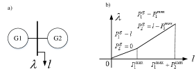
Figure 3: The policy curve of a single bus load with two generators.

IV-B The Derivation of Price-Demand Policy

Given the SCED problem in (1), the goal of this subsection is to derive the policy between the LMP vector $\bm{\lambda}$ and the load vector $\bm{l}$. Let $\bm{I}\in\mathbb{R}^{|\mathcal{N}|\times|\mathcal{N}|}$ be the identity matrix. Before going to the details, we firstly rewrite the SCED problem in (1) into the compact form of a quadratic programming (QP) problem

$$\mathop{\min}_{\bm{P^{g}}}\frac{1}{2}(\bm{P}^{g})^{\top}\bm{Q}(\bm{P}^{g})+\bm{q}^{\top}\bm{P}^{g}+\sum_{i\in\mathcal{N}}c_{i}^{g}$$ (5a)

$$s.t.\bm{1}_{|\mathcal{N}|}^{\top}\bm{P}^{g}=\bm{1}_{|\mathcal{N}|}^{\top}\bm{l}:\gamma$$ (5b)

$$\quad\ \bm{A}\bm{P}^{g}\leq\bm{b}:\bm{\mu}$$ (5c)

$$\quad\ \bm{S}\bm{P}^{g}\leq\bm{h}:\bm{\psi},$$ (5d)

where

$$\bm{Q}=\begin{bmatrix}a_{1}^{g}&&\\ &\ddots&\\ &&a_{|\mathcal{N}|}^{g}\end{bmatrix},\bm{q}=\begin{bmatrix}b_{1}^{g}\\ \vdots\\ b_{|\mathcal{N}|}^{g}\end{bmatrix},\bm{A}=\begin{bmatrix}\bm{H}\\ -\bm{H}\\ \end{bmatrix},$$

$$\bm{b}=\begin{bmatrix}\ \bm{f}+\bm{H}\bm{l}\ \\ \ \bm{f}-\bm{H}\bm{l}\end{bmatrix},\bm{S}=\begin{bmatrix}\bm{I}\\ -\bm{I}\\ \end{bmatrix},\bm{\mu}=\begin{bmatrix}\bm{\mu}_{2}\\ \bm{\mu}_{1}\\ \end{bmatrix},\bm{\psi}=\begin{bmatrix}\bm{\psi}_{2}\\ \bm{\psi}_{1}\\ \end{bmatrix},$$

$$\bm{h}_{1}=\begin{bmatrix}-P^{min}_{1}\\ \vdots\\ -P^{min}_{|\mathcal{N}|}\\ \end{bmatrix},\bm{h}_{2}=\begin{bmatrix}P^{max}_{1}\\ \vdots\\ P^{max}_{|\mathcal{N}|}\\ \end{bmatrix},\bm{h}=\begin{bmatrix}\bm{h}_{2}\\ \bm{h}_{1}\\ \end{bmatrix}.$$

We now proceed with the following theorem to characterize the relationship between optimization input parameters $\bm{l}$ and the optimal solutions.

Theorem 1 [26]: Consider the parameters of QP problem belong to a convex set and the parameters $\bm{Q}$ is positive definite. The optimal solution of QP problem is given by a conditional piecewise linear function of the varying parameters.

We can have the corollary from the Theorem 1 that in the neighborhood of a point of the optimal solution, the mapping between the optimal solution and the load is an affine function. Therefore, we can have the following proposition for the QP problem in (5).

Proposition 1: Consider the QP problem (5). Let $\bm{P}^{g}(\bm{l}),\gamma(\bm{l}),\bm{\mu}(\bm{l}),\bm{\psi}(\bm{l})$ denote the mapping between the load $\bm{l}$ and the optimal solutions of primal and dual variables, $\bm{P}^{g}(\tilde{\bm{l}}),\gamma(\tilde{\bm{l}}),\bm{\mu}(\tilde{\bm{l}}),\bm{\psi}(\tilde{\bm{l}})$ denote the optimal primal and dual solutions under a given point $\tilde{\bm{l}}$. The calculation of $\bm{P}^{g}(\bm{l}),\gamma(\bm{l}),\bm{\mu}(\bm{l}),\bm{\psi}(\bm{l})$, in the neighborhood of $\bm{l}=\tilde{\bm{l}}$, is

$$\begin{bmatrix}\bm{P}^{g}(\bm{l})\\ \gamma(\bm{l})\\ \bm{\mu}(\bm{l})\\ \bm{\psi}(\bm{l})\end{bmatrix}=\begin{bmatrix}\bm{P}^{g}(\tilde{\bm{l}})\\ \gamma(\tilde{\bm{l}})\\ \bm{\mu}(\tilde{\bm{l}})\\ \bm{\psi}(\tilde{\bm{l}})\end{bmatrix}+(\bm{M}_{0})^{-1}\cdot\bm{N}_{0}\cdot(\bm{l}-\tilde{\bm{l}}),$$ (6)

where $\bm{M}_{0}\in\mathbb{R}^{(3|\mathcal{N}|+1+2|\mathcal{A}|)\times(3|\mathcal{N}|+1+2|\mathcal{A}|)}$ and $\bm{N}_{0}\in\mathbb{R}^{(3|\mathcal{N}|+1+2|\mathcal{A}|)\times|\mathcal{N}|}:$

$$\bm{M}_{0}=$$

$$\begin{bmatrix}\bm{Q}&\bm{1}_{|\mathcal{N}|}&\bm{A}^{\top}&\bm{S}^{\top}\\ \bm{1}_{|\mathcal{N}|}^{\top}&0&0&0\\ D(\bm{\mu}(\tilde{\bm{l}}))\bm{A}&\bm{0}&D(\bm{A}\bm{P}^{g}(\tilde{\bm{l}})-\bm{b})&\bm{0}\\ D(\bm{\psi}(\tilde{\bm{l}}))\bm{S}&\bm{0}&\bm{0}&D(\bm{S}\bm{P}^{g}(\tilde{\bm{l}})-\bm{h})\\ \end{bmatrix};$$

$$\bm{N}_{0}=\begin{bmatrix}\bm{0}\\ \bm{1}_{|\mathcal{N}|}^{\top}\\ D(\bm{\mu}(\tilde{\bm{l}}))\begin{bmatrix}\bm{H}\\ -\bm{H}\end{bmatrix}\bm{I}\\ \bm{0}\end{bmatrix}.$$

$D(\cdot)$ creates a diagonal matrix from a vector. The proof of Proposition 1 is given in Appendix A.

Once (6) is obtained, we can find the optimal primal and dual variables’ values starting from $\tilde{\bm{l}}$. According to (2), the policy $\pi(\bm{l})$ in the neighborhood of $\tilde{\bm{l}}$ can be derived as

$$\pi(\bm{l})=\gamma(\bm{l})\cdot\bm{1}_{|\mathcal{N}|}-\bm{H}^{T}[\bm{\mu}_{2}(\bm{l})-\bm{\mu}_{1}(\bm{l})].$$ (7)

Recall in the DR targeting task, we are interested in finding LMPs given varying demand vectors. Such task then motivates us to firstly identify $\pi(\bm{l})$ for a specific $\tilde{\bm{l}}$ using (7), and then to work through all possible load regions that have distinct policy parameters defined by (6).

The neighborhood of $\tilde{\bm{l}}$ where the (6) holds is defined as the critical region $\mathcal{B}(\tilde{\bm{l}})$. Since the sign of the optimal dual solutions $\bm{\mu}(\bm{l}),\bm{\psi}(\bm{l})$ in (6) is the same within the region, the active inequalities and the inactive inequalities remain the same as well. Let $\tilde{\bm{A}},\tilde{\bm{b}}$, $\tilde{\bm{S}}$, and $\tilde{\bm{h}}$ denote the coefficients corresponding to the inactive inequalities, and $\tilde{\bm{\mu}}(\bm{l}),\tilde{\bm{\psi}}(\bm{l})$ be part of the $\bm{\mu}(\bm{l}),\bm{\psi}(\bm{l})$ corresponding to the active inequalities. Feasibility is ensured by substituting $\bm{P}^{g}(\bm{l})$ into the inactive inequalities and the equality in (5b), whereas the optimality condition is given by $\tilde{\bm{\mu}}(\bm{l})\geq 0,\tilde{\bm{\psi}}(\bm{l})\geq 0$. The critical region $\mathcal{B}(\tilde{\bm{l}})$ is defined as

$$\begin{split}\tilde{\mathcal{B}}(\tilde{\bm{l}})=\{&\tilde{\bm{A}}\bm{P}^{g}(\bm{l})\leq\tilde{\bm{b}},\tilde{\bm{S}}\bm{P}^{g}(\bm{l})\leq\tilde{\bm{h}},\bm{1}_{|\mathcal{N}|}^{\top}\bm{P}^{g}(\bm{l})=\bm{1}_{|\mathcal{N}|}^{\top}\bm{l},\\ &\qquad\qquad\tilde{\bm{\mu}}(\bm{l})\geq 0,\tilde{\bm{\psi}}(\bm{l})\geq 0,\mathcal{L}\};\\ &\mathcal{B}(\tilde{\bm{l}})=\triangle\{\tilde{\mathcal{B}}(\tilde{\bm{l}})\},\end{split}$$ (8)

where $\mathcal{L}$ denotes the given initial convex set of all feasible vectors of loads, and $\triangle\{\cdot\}$ is defined as an operator which removes redundant constraints; see [29]. Once $\mathcal{B}(\tilde{\bm{l}})$ has been obtained, the rest of region $\mathcal{N}(\tilde{\bm{l}})$ is obtained; see [30]:

$$\mathcal{N}(\tilde{\bm{l}})=\mathcal{L}-\mathcal{B}(\tilde{\bm{l}}).$$ (9)

Given the remaining regions $\mathcal{N}(\tilde{\bm{l}})$, the mapping between load to generation $\bm{P}^{g}(\bm{l})$, the LMP policy $\pi(\bm{l})$, and the corresponding critical region $\mathcal{B}(\tilde{\bm{l}})$ can then been obtained via Proposition 1 iteratively. The algorithm terminates when there are no more regions to explore. The main steps of the algorithm is summarized in Algorithm 1.

To sum up, the policy $\pi(\bm{l})$ on the convex set of feasible load vector $\mathcal{L}$ is also a piecewise linear function, where the function is affine on each critical region which can be characterized by a high-dimensional polytope. With this representation of the policy $\pi(\bm{l})$, the DR targeting problem formulated in (3) can be solved separately on each critical region with the policy represented by an affine function. This resolves the burden on finding LMPs and solving DR targeting problem simultaneously in an optimization problem. And a constraint regarding the space of the critical region is therefore added to the original problem. We will illustrate the overall solution procedure in the next Section.

Algorithm 1 The derivation of policy $\pi(\bm{l})$ via multi-parametric quadratic programming

1:The initial set of all feasible vector of loads $\mathcal{L}$

2:In the given set of $\mathcal{L}$, solve (5) by treating $\bm{l}$ as a free variable to obtain a feasible point $\tilde{\bm{l}}$.

3:Fix $\bm{l}=\tilde{\bm{l}}$ and solve (5) to obtain $\bm{P}^{g}(\tilde{\bm{l}}),\gamma(\tilde{\bm{l}}),\bm{\mu}(\tilde{\bm{l}}),\bm{\psi}(\tilde{\bm{l}})$.

4:Compute $(\bm{M}_{0})^{-1}\cdot\bm{N}_{0}$ and obtain $\bm{P}^{g}(\bm{l}),\gamma(\bm{l}),\bm{\mu}(\bm{l}),\bm{\psi}(\bm{l})$ from (6).

5:Compute the policy $\pi(\bm{l})$ from (7).

6:Obtain the critical region $\mathcal{B}(\tilde{\bm{l}})$ as defined in (8).

7:Obtain $\mathcal{N}(\tilde{\bm{l}})$ using (9).

8:If no more regions to explore, go to next step, otherwise given $\mathcal{N}(\tilde{\bm{l}})$, solve (5) by treating $\bm{l}$ as a free variable to obtain a new feasible point $\tilde{\bm{l}}$, and then go to Step 2.

9:Collect all the solutions and unify the regions having the same solution to obtain a compact representation.

V The Solution Strategy for DR Targeting Problem

Given the derived policy $\pi(\bm{l})$, in this section, we show that the DR targeting problem can be formulated as a MIQP problem. And an acceleration strategy for the solution process is also given.

With the policy $\pi(\bm{l})$, let the set of polytopes characterized the initial set $\mathcal{L}$ denote as $\mathcal{M}$. For any polytope $m\in\mathcal{M}$, the corresponding policy $\pi_{m}(\bm{l})$ is an affine function. Here, we denote the region of the polytope as $\bm{R}_{m}\cdot\bm{l}\leq\bm{r}_{m}$ for polytope $m$. Therefore, the DR targeting problem under the polytope $m$ is a MIQP problem, given by

$$\mathop{\min}_{\bm{v},\bm{x}}(\sum_{i\in\mathcal{N}}\lambda_{i}-|\mathcal{N}|\cdot\lambda^{*})^{2}+\bm{w}^{\top}\bm{x}$$ (10a)

$$s.t.\eqref{3(b)},\eqref{3(c)},\eqref{3(d)}$$

$$\quad\ \bm{\lambda}=\pi_{m}(\bm{\hat{l}})$$ (10b)

$$\quad\ \bm{R}_{m}\cdot\bm{\hat{l}}\leq\bm{r}_{m}.$$ (10c)

Although we can solve the MIQP problem for each $m\in\mathcal{M}$, and return the optimal solution of the problem whose optimal objective is the smallest among the $|\mathcal{M}|$ problems, this practice is computationally expensive, as solving the MIQP problem takes a relatively long time for multiple polytopes. Considering the fact that the allowable demand reduction is upper bounded, there are only a set of polytopes contain feasible solutions for the MIQP problem. While these polytopes only take up a small portion among the $|\mathcal{M}|$ problems, we can greatly reduce the time of solving the DR targeting by only working on feasible DR regions. To accelerate the process, we propose to firstly judge the feasibility of (10) before solving it. As such, the time of solving the infeasible MIQP problem is spared. Therefore, the relaxed version of (10) is firstly solved to help judge the feasibility, which is given by

$$\mathop{\min}_{\bm{v},\bm{x}}(\sum_{i\in\mathcal{N}}\lambda_{i}-|\mathcal{N}|\cdot\lambda^{*})^{2}+\bm{w}^{\top}\bm{x}$$ (11a)

$$s.t.\eqref{3(c)},\eqref{3(d)}$$

$$\quad\ 0\leq v_{i}\leq 1,\forall i\in\mathcal{N}$$ (11b)

$$\quad\ \bm{\lambda}=\pi_{m}(\bm{\hat{l}})$$ (11c)

$$\quad\ \bm{R}_{m}\cdot\bm{\hat{l}}\leq\bm{r}_{m},$$ (11d)

where the binary variable $v_{i}$ is relaxed to be a continuous variable in the range of $[0,1]$. As $v_{i}$ is a continuous variable in (11), the constraint (3b) which bounds the number of DR locations is omitted. If the relaxed problem in (11) is feasible, then solve the MIQP problem in (10); otherwise go to the problem on the next polytope. The pseudocode regarding the solution strategy is summarized in Algorithm 2.

Algorithm 2 The solution strategy for DR targeting

1:The derived policy $\pi(\bm{l})$, which is defined on the region formed by a set of polytopes $\mathcal{M}$, and for each polytope $m\in\mathcal{M}$, the policy is an affine function defined as $\pi_{m}(\bm{l})$.

2:for $m\in\mathcal{M}$ do

3:     Given the policy $\pi_{m}(\hat{\bm{l}})$ and the corresponding polytope $\bm{R}_{m}\cdot\bm{\hat{l}}\leq\bm{r}_{m}$, solve the relaxed problem in (11).

4:     If (11) is feasible, then solve the MIQP problem in (10). If the MIQP problem in (10) is feasible, then store the optimal solution and objective in the buffer.

5:end for

6:Return the optimal solution whose optimal objective is the smallest in the buffer.

VI Case Study

This section testifies the effectiveness of the proposed approach on New England IEEE 39-Bus system [31]. And the aim is to show the proposed approach (1) can reduce the averaged LMPs to the reference point with smaller demand reduction compared to heuristics such as selecting DR locations with highest LMPs; (2) achieves efficient DR targeting under different number of DR locations and different value of weight vector $\bm{w}$; (3) can achieve effective policies even when network parameters are inaccurate. Lastly, to showcase the proposed approach is also generalizable to other DR applications, we consider the case of load shifting and show the proposed approach can still effectively reduce the average LMPs.

We adapt the scale of parameters in the standard IEEE 39-Bus system and the detailed configurations are provided along with the codes. In addition, without the special statement, the nodal demand levels $\bm{l}_{0}$ and nodal LMPs before DR used in the subsequent subsections are the ones illustrated in Fig. 4.

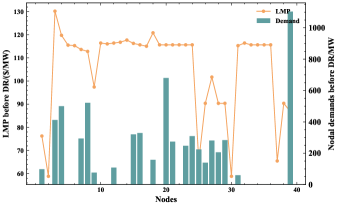
Figure 4: The nodal demand levels and nodal LMPs before DR.

VI-A Operational Advantage of the Proposed Approach

In this subsection, we set the number of targeted DR nodes $K$ in (3b) as 5, the reference value of LMP as 70 $/MW, and every element in the weight vector $\bm{w}$ as 1.1. As the LMP at each node can be interpreted as an extra cost when an additional one more unit of nodal demand, it is a straightforward choice to reduce the demand at nodes with relatively high LMPs in order to lower the system averaged LMP. Therefore, we chose this method as a benchmark algorithm, and under such node selection policy, #3, #4, #12, #15, #18 are selected as locations for implementing DR.

The averaged LMP and total demand reduction in the system are shown in Fig. 5 and the nodal LMP after DR is shown in Fig. 6. Both the proposed approach and the comparison candidate can reduce the averaged LMP to the reference point. The nodal LMPs of the proposed approach vary around 70 $/MWh, and the nodal LMPs of the comparison candidate are of the same value, which indicates there is no network congestion after DR. However, the proposed approach requires less total demand reduction compared with the benchmarking method and the reduction quantity only takes up to 4.7% in the system demand level, indicating the superiority of the proposed approach. Therefore, the results reveal that the ideal nodes to implement DR are not necessarily coinciding with the nodes with highest LMPs, which is reasonable as the comparison candidate produces a feasible solution to the proposed MIQP problem in (10), not an optimal one. The results demonstrate that the proposed approach can bring more advantages to the operation than the comparison candidate.

Furthermore, the targeted nodes of the two approaches and the corresponding demand reduction (shown in the parentheses) are displayed in Table I. Interestingly, except for the node #3, the nodes with the highest LMPs are not selected as DR locations by the proposed method. And the node with the relatively low LMP value is chosen, for example the node #25. Also, the targeted nodes of the proposed method are not necessarily the load centers with heavy demand. For instance, the node #1 is selected, whose demand is relatively small. The results further show that the intuitive wisdom is not necessarily the optimal one. And the rigorous examination is needed to target the proper nodes for more effective DR.

Table I: The index of targeted nodes and corresponding demand reduction (in MW).

Proposed	#1(33)	#3(85)	#20(120)	#25(45)	#39(30)
Comparison	#3(84)	#4(120)	#12(25)	#15(65)	#18(28)

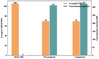
Figure 5: The comparison between the proposed and the DR targeting method selecting the targeted nodes with the highest LMP.

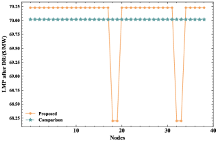
Figure 6: Nodal LMP of the proposed approach and comparison candidate after DR.

Also, by testing the proposed approach and comparing candidate on different demand levels before DR, we aim to show that the proposed approach is superior to the method where DR is implemented at fixed nodes. Specifically, we test the approach on eight kinds of different nodal demand levels before DR, which are denoted as $S_{1}-S_{8}$. Those demand levels are generated by adding the Gaussian noise to the demand level shown in Fig. 4. The comparison candidate always selects the nodes #3, #4, #12, #15, #18 as DR locations, whose corresponding LMPs are almost the highest in the system. The results regarding the demand reduction are given in Table II, where the sign of $-$ indicates the problem is infeasible, which means given the targeted nodes, the constraint (10c) cannot be satisfied in any of the problem. In other words, the demand level $\hat{\bm{l}}$ after DR cannot fall in the region of any polytope in the set $\mathcal{M}$. Since for feasible instances, the methods can always reduce the averaged LMP to the reference value, namely 70 $/MWh, the results regarding the averaged LMPs after DR are not shown in Table II. Among $S_{1}-S_{8}$, the comparison method is infeasible in six problems and results in larger demand reduction in the remaining problems, compared with the proposed approach. For the proposed approach, the targeted nodes in $S_{1}-S_{8}$ are shown in Table III. The targeted nodes differ from each other with the variation of the demand levels before DR. And we note that in $S_{7}$, it only needs four targeted nodes to lower the averaged LMP. The results validate that the proposed approach can adapt the DR targeted nodes to different demand levels, which is superior to the approach of choosing the fixed nodes.

Table II: Total demand reduction (in MW) under different nodal demand levels before DR. “-” denotes infeasible DR decisions.

	$S_{1}$	$S_{2}$	$S_{3}$	$S_{4}$	$S_{5}$	$S_{6}$	$S_{7}$	$S_{8}$
Proposed	326	343	353	336	322	319	307	339
Comparison	-	-	-	-	333	-	317	-

Table III: Targeted nodes of the proposed approach under different nodal demand levels before DR.

$S_{1}$	#3	#20	#29	#31	#39
$S_{2}$	#1	#3	#20	#31	#39
$S_{3}$	#3	#7	#20	#31	#39
$S_{4}$	#3	#7	#20	#31	#39
$S_{5}$	#1	#3	#20	#25	#39
$S_{6}$	#1	#3	#7	#20	#25
$S_{7}$	#1	#3	#20	#25	-
$S_{8}$	#3	#7	#20	#31	#39

Furthermore, to validate the feasibility judgement in Algorithm 2 can accelerate the computation process, we compare it with the method which solves (10) directly without firstly judging the feasibility. The computation time under different values of the integer $K$ is given in Table IV. It demonstrates that the proposed approach can reduce the computation time, as the number of feasible problems takes up a small fraction of all the problems. This sheds light on implementing DR targeting in practice which has a limitation on computation time.

Table IV: Computation time comparison undering varing $K$.

	$K=2$	$K=5$	$K=10$
Proposed	152s	109s	130s
Original	328s	333s	365s

VI-B Investigation on Different Targeted Node Numbers and Weight Values

The number of the targeted nodes, which is controlled by the integer $K$ in (3b), has impact on the DR performance. Likewise, the value of the weight $\bm{w}$ controls the balance between averaged LMP reduction and demand reduction. Therefore, we investigate the influence of those parameters in this subsection. Specifically, the reference value of LMP is set as 60 $/MW, and the number of targeted nodes is set as 2, 5, and 10. The elements in the weight vector are set as 1.1 and 111, respectively. The results in Fig. 7 show that with the increasing number of the targeted nodes, the averaged LMP can be reduced to a lower value. Concretely, when the number of the targeted nodes is set as 2 or 5, the averaged LMP cannot be reduced to the reference point, and different values of weight have no impact on the results. When the number of the targeted nodes is set as 10, with less weight imposed on the total demand reduction, the proposed approach can reduce the averaged LMP to the reference point by reducing more demands. In contrast, with larger weight, the larger demand reduction is punished more. Therefore, the averaged LMP is higher than the reference point and the corresponding demand reduction is smaller.

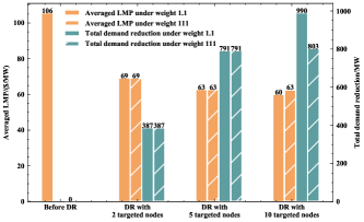
Figure 7: Averaged LMP and total demand reduction under different number of targeted nodes and value of weight.

VI-C Investigation on the Influence of Inaccurate System Parameters

Due to the measurement error, it is likely that the system parameters, used for deriving the policy, are different from the actual ones. To investigate the influence of the inaccurate system parameters on the DR targeting results, we consider two inaccurate policies built by the inaccurate transmission limits, namely $\bm{\hat{f}}_{1}=0.9\bm{f}$ and $\bm{\hat{f}}_{2}=1.1\bm{f}$, where $\bm{f}$ denotes the original line flow limits. And we denote the policies built under $\bm{\hat{f}}_{1}$ and $\bm{\hat{f}}_{2}$ as policy 1 and policy 2 in the following discussion. The results under the policy based on the accurate parameters and the results under policy 1 and policy 2 are shown in Fig. 8, where the number of the targeted nodes is set as 5 and the element in the weight vector $\bm{w}$ is set as 1.1. The reference value of LMP is set as 70 $/MW and 60 $/MW, respectively. For the first LMP reference value, the averaged LMP can be reduced to the reference point. However, for the second one, it cannot be reduced to the reference point with only 5 targeted nodes. For the two reference values of LMP, the values of the averaged LMP after optimization, which relies on the accurate policy and the inaccurate policies respectively, are almost the same. The only difference is that the total demand reduction under policy 2 is slightly larger than that under the accurate one, when the reference point is set as 70$/MW. The results show that the impact of the inaccurate parameters on the results is relatively small, and the proposed approach can still achieve the good performance under the policy built by the inaccurate system parameters.

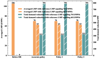
Figure 8: Averaged LMP and total demand reduction under the policies built by the accurate and inaccurate system parameters.

VI-D Application on Targeted Load Shifting

To showcase the proposed framework is also applicable to other DR applications, we consider the case of load shifting in this subsection. The objective is to reduce average LMPs by geographically shifting load from one node to another while the net demand keeps constant. Such DR type can be achieved by the cooperation between ISO and a group of geographically flexible demand such as data centers [32, 33]. Tailored to the case of load shifting, the MIQP formulation in (10) is slightly modified by adding a constraint ensuring the total demand reduction to be zero.

$$\mathop{\min}_{\bm{v},\bm{x}}(\sum_{i\in\mathcal{N}}\lambda_{i}-|\mathcal{N}|\cdot\lambda^{*})^{2}$$ (12)

$$s.t.\eqref{3(b)},\eqref{3(c)},\eqref{3(d)}$$

$$\quad\ \bm{\lambda}=\pi_{m}(\bm{\hat{l}})$$

$$\quad\ \bm{R}_{m}\cdot\bm{\hat{l}}\leq\bm{r}_{m}$$

$$\quad\ \bm{1}_{|\mathcal{N}|}^{\top}\bm{x}=0.$$

The number of the targeted nodes are chosen as 2, 5, 8, and 10 respectively. And the reference value of LMP and the elements in the weight are set as 70$/MW and $1.1$ respectively. The averaged LMP under the different number of targeted nodes is shown in Fig. 9. Although the total demand reduction remains zero, the average LMP can drop below 100 $/MWh by changing the load distribution of the system. And it can be further decreased by increasing the number of DR targeted nodes. Therefore, the results show that the proposed approach is also applicable to other DR types by finding the most effective demand nodes to reduce the overall costs.

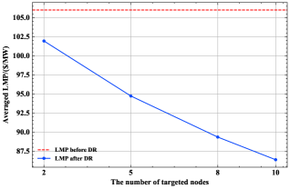
Figure 9: Averaged LMP under different number of targeted nodes in a load shifting DR event.

VII Conclusion

In this work, we propose an efficient DR targeting approach implemented by a system operator to target proper nodes as locations for implementing DR, and the proposed scheme can efficiently determine the corresponding nodes’ demand reduction quantity. Such a DR targeting algorithm can reduce the averaged LMPs to a reference point with mild load reductions. The theoretical relationship between the nodal LMPs and nodal demands is derived, such that the DR targeting problem is formulated as a rigorous MIQP problem, where the demand reduction serves as the “action knob” to control the LMP. A solution strategy is also proposed to improve the computational efficiency for solving the DR targeting problem.

Case studies reveal that the common heuristic of choosing nodes with the highest LMPs to implement DR is not optimal. The proposed approach can achieve the same averaged LMP reduction with a smaller demand reduction. Also, its performance is validated under varying settings of the number of targeted nodes and the weight vector. Furthermore, the experiment shows that the proposed approach can achieve almost the same performance under accurate and inaccurate system parameters, and is applicable to other DR types, such as load shifting.

Our approach can inform system operators how to target nodes for price reduction under constrained budgets. As the nodes with the highest LMPs are not necessarily the optimal locations for DR, they are “free-riders” by enjoying the LMP reduction through the demand reduction in other nodes. Thus, future directions about DR mechanism design will include fairness notions regarding customer groups and the uncertainties about both generation and nodal demands. We will also explore more efficient learning approaches to find the LMP policies.

Appendix A Proof of Proposition 1

Proof.

The Lagrangian of (5) is given by

$$\begin{split}&L=\frac{1}{2}(\bm{P}^{g})^{\top}\bm{Q}(\bm{P}^{g})+\bm{q}^{\top}\bm{P}^{g}+\sum_{i\in\mathcal{N}}c_{i}^{g}+\\ &\gamma(\bm{1}_{|\mathcal{N}|}^{\top}\bm{P}^{g}-\bm{1}_{|\mathcal{N}|}^{\top}\bm{l})+\bm{\mu}^{\top}(\bm{A}\bm{P}^{g}-\bm{b})+\bm{\psi}^{\top}(\bm{S}\bm{P}^{g}-\bm{h})\end{split}$$ (13)

Given the optimal solution of primal and dual variables when $\bm{l}=\tilde{\bm{l}}$, namely $\bm{P}^{g}(\tilde{\bm{l}}),\gamma(\tilde{\bm{l}}),\bm{\mu}(\tilde{\bm{l}}),\bm{\psi}(\tilde{\bm{l}})$, the KKT conditions for stationarity, primal feasibility, and complementary slackness are

$$\bm{Q}\bm{P}^{g}(\tilde{\bm{l}})+\bm{q}+\gamma(\tilde{\bm{l}})\bm{1}_{|\mathcal{N}|}+\bm{A}^{\top}\bm{\mu}(\tilde{\bm{l}})+\bm{S}^{\top}\bm{\psi}(\tilde{\bm{l}})=0$$ (14a)

$$\bm{1}_{|\mathcal{N}|}^{\top}\bm{P}^{g}(\tilde{\bm{l}})-\bm{1}_{|\mathcal{N}|}^{\top}\bm{l}=0$$ (14b)

$$D(\bm{\mu}(\tilde{\bm{l}}))(\bm{A}\bm{P}^{g}(\tilde{\bm{l}})-\bm{b})=0$$ (14c)

$$D(\bm{\psi}(\tilde{\bm{l}}))(\bm{S}\bm{P}^{g}(\tilde{\bm{l}})-\bm{h})=0$$ (14d)

Taking the differentials of these conditions gives the equations

$$(d\bm{Q})\bm{P}^{g}(\tilde{\bm{l}})+\bm{Q}(d\bm{P}^{g})+d\bm{q}+d\gamma\bm{1}_{|\mathcal{N}|}+$$

$$\quad(d\bm{A})^{\top}\bm{\mu}(\tilde{\bm{l}})+\bm{A}^{\top}(d\bm{\mu})+(d\bm{S})^{\top}\bm{\psi}(\tilde{\bm{l}})+\bm{S}^{\top}(d\bm{\psi})=0$$ (15a)

$$\bm{1}_{|\mathcal{N}|}^{\top}d\bm{P}^{g}-\bm{1}_{|\mathcal{N}|}^{\top}d\bm{l}=0$$ (15b)

$$D(\bm{A}\bm{P}^{g}(\tilde{\bm{l}})-\bm{b})d\bm{\mu}+$$

$$\qquad D(\bm{\mu}(\tilde{\bm{l}}))[(d\bm{A})\bm{P}^{g}(\tilde{\bm{l}})+\bm{A}(d\bm{P}^{g})-d\bm{b}]=0$$ (15c)

$$D(\bm{S}\bm{P}^{g}(\tilde{\bm{l}})-\bm{h})d\bm{\psi}+$$

$$\qquad D(\bm{\psi}(\tilde{\bm{l}}))[(d\bm{S})\bm{P}^{g}(\tilde{\bm{l}})+\bm{S}(d\bm{P}^{g})-d\bm{h}]=0.$$ (15d)

We rewrite (15) into a compact matrix form

$$\begin{split}&\begin{bmatrix}\bm{Q}&\bm{1}_{|\mathcal{N}|}&\bm{A}^{\top}&\bm{S}^{\top}\\ \bm{1}_{|\mathcal{N}|}^{\top}&0&0&0\\ D(\bm{\mu}(\tilde{\bm{l}}))\bm{A}&\bm{0}&D(\bm{A}\bm{P}^{g}(\tilde{\bm{l}})-\bm{b})&\bm{0}\\ D(\bm{\psi}(\tilde{\bm{l}}))\bm{S}&\bm{0}&\bm{0}&D(\bm{S}\bm{P}^{g}(\tilde{\bm{l}})-\bm{h})\\ \end{bmatrix}\cdot\begin{bmatrix}d\bm{P}^{g}\\ d\gamma\\ d\bm{\mu}\\ d\bm{\psi}\end{bmatrix}\\ &=\begin{bmatrix}-d\bm{Q}\bm{P}^{g}(\tilde{\bm{l}})-d\bm{q}-(d\bm{A})^{\top}\bm{\mu}(\tilde{\bm{l}})-(d\bm{S})^{\top}\bm{\psi}(\tilde{\bm{l}})\\ \bm{1}_{|\mathcal{N}|}^{\top}d\bm{l}\\ -D(\bm{\mu}(\tilde{\bm{l}}))(d\bm{A})\bm{P}^{g}(\tilde{\bm{l}})+D(\bm{\mu}(\tilde{\bm{l}}))d\bm{b}\\ -D(\bm{\psi}(\tilde{\bm{l}}))(d\bm{S})\bm{P}^{g}(\tilde{\bm{l}})+D(\bm{\psi}(\tilde{\bm{l}}))d\bm{h}\end{bmatrix}\end{split}$$ (16)

The coefficient matrix in the left-hand side is the matrix $\bm{M}_{0}$. Since we wish to compute the Jacobian $\frac{\partial\bm{P}^{g}}{\partial\bm{l}},\frac{\partial\gamma}{\partial\bm{l}},\frac{\partial\bm{\mu}}{\partial\bm{l}},\frac{\partial\bm{\psi}}{\partial\bm{l}}$, we simply substitute $d\bm{l}=\bm{I}$, and set all other differential terms in the right-hand side to zero. Given

$$d\bm{b}=\begin{bmatrix}d\bm{f}+(d\bm{H})\bm{l}+\bm{H}d\bm{l}\\ d\bm{f}-(d\bm{H})\bm{l}-\bm{H}d\bm{l}\end{bmatrix}$$

Then the right-hand vector become

$$\begin{bmatrix}\bm{0}\\ \bm{1}_{|\mathcal{N}|}^{\top}\\ D(\bm{\mu}(\tilde{\bm{l}}))\begin{bmatrix}\bm{H}\\ -\bm{H}\end{bmatrix}\bm{I}\\ \bm{0}\end{bmatrix},$$

which is $\bm{N}_{0}$. Therefore, we have

$$\begin{bmatrix}\frac{\partial\bm{P}^{g}}{\partial\bm{l}}\\ \frac{\partial\gamma}{\partial\bm{l}}\\ \frac{\partial\bm{\mu}}{\partial\bm{l}}\\ \frac{\partial\bm{\psi}}{\partial\bm{l}}\end{bmatrix}=\bm{M}_{0}^{-1}\bm{N}_{0}$$ (17)

With the Theorem 1 and the Jacobian derived in (17), the calculation of $\bm{P}^{g}(\bm{l}),\gamma(\bm{l}),\bm{\mu}(\bm{l}),\bm{\psi}(\bm{l})$, in the neighborhood of $\bm{l}=\tilde{\bm{l}}$ is the affine function defined in (6), which completes the proof.

∎

References

- [1] C. W. Gellings and J. H. Chamberlin, “Demand-side management: concepts and methods,” 1987.
- [2] J. S. Vardakas, N. Zorba, and C. V. Verikoukis, “A survey on demand response programs in smart grids: Pricing methods and optimization algorithms,” IEEE Communications Surveys & Tutorials, vol. 17, no. 1, pp. 152–178, 2014.
- [3] H. Yang, J. Zhang, J. Qiu, S. Zhang, M. Lai, and Z. Y. Dong, “A practical pricing approach to smart grid demand response based on load classification,” IEEE Transactions on Smart Grid, vol. 9, no. 1, pp. 179–190, 2016.
- [4] C. Chen, J. Wang, and S. Kishore, “A distributed direct load control approach for large-scale residential demand response,” IEEE Transactions on Power Systems, vol. 29, no. 5, pp. 2219–2228, 2014.
- [5] B. Ramanathan and V. Vittal, “A framework for evaluation of advanced direct load control with minimum disruption,” IEEE Transactions on Power Systems, vol. 23, no. 4, pp. 1681–1688, 2008.
- [6] H. Zhong, L. Xie, and Q. Xia, “Coupon incentive-based demand response: Theory and case study,” IEEE Transactions on Power Systems, vol. 28, no. 2, pp. 1266–1276, 2012.
- [7] R. Lu and S. H. Hong, “Incentive-based demand response for smart grid with reinforcement learning and deep neural network,” Applied energy, vol. 236, pp. 937–949, 2019.
- [8] “Number of customers enrolled in demand response electricity programs in the united states in 2020, by sector,” https://www.statista.com/statistics/669480/electricity-demand-response-customers-in-the-us/, accessed: 2022-10-21.
- [9] D. S. Kirschen and G. Strbac, Fundamentals of power system economics. John Wiley & Sons, 2018.
- [10] X. Fang, Q. Hu, F. Li, B. Wang, and Y. Li, “Coupon-based demand response considering wind power uncertainty: A strategic bidding model for load serving entities,” IEEE Transactions on Power Systems, vol. 31, no. 2, pp. 1025–1037, 2015.
- [11] J. MacDonald, P. Cappers, D. Callaway, and S. Kiliccote, “Demand response providing ancillary services: A comparison of opportunities and challenges in us wholesale markets,” 2022.
- [12] J. Torriti, M. G. Hassan, and M. Leach, “Demand response experience in europe: Policies, programmes and implementation,” Energy, vol. 35, no. 4, pp. 1575–1583, 2010.
- [13] H. Zhong, L. Xie, Q. Xia, C. Kang, and S. Rahman, “Multi-stage coupon incentive-based demand response in two-settlement electricity markets,” in 2015 IEEE Power & Energy Society Innovative Smart Grid Technologies Conference (ISGT). IEEE, 2015, pp. 1–5.
- [14] E. Dehnavi and H. Abdi, “Determining optimal buses for implementing demand response as an effective congestion management method,” IEEE Transactions on Power Systems, vol. 32, no. 2, pp. 1537–1544, 2016.
- [15] M. H. Moradi, A. R. Reisi, and S. M. Hosseinian, “An optimal collaborative congestion management based on implementing dr,” IEEE Transactions on Smart Grid, vol. 9, no. 5, pp. 5323–5334, 2017.
- [16] D. Yang and Y. Chen, “Demand response and market performance in power economics,” in 2009 IEEE Power and Energy Society General Meeting, 2009, pp. 1–6.
- [17] L. Wu, “Impact of price-based demand response on market clearing and locational marginal prices,” IET Generation, Transmission & Distribution, vol. 7, no. 10, pp. 1087–1095, 2013.
- [18] X. Wang, F. Li, J. Dong, M. M. Olama, Q. Zhang, Q. Shi, B. Park, and T. Kuruganti, “Tri-level scheduling model considering residential demand flexibility of aggregated hvacs and evs under distribution lmp,” IEEE Transactions on Smart Grid, vol. 12, no. 5, pp. 3990–4002, 2021.
- [19] L. Chen, N. Li, S. H. Low, and J. C. Doyle, “Two market models for demand response in power networks,” in 2010 First IEEE International Conference on Smart Grid Communications. IEEE, 2010, pp. 397–402.
- [20] K. Lee, X. Geng, S. Sivaranjani, B. Xia, H. Ming, S. Shakkottai, and L. Xie, “Targeted demand response for mitigating price volatility and enhancing grid reliability in synthetic texas electricity markets,” iScience, vol. 25, no. 2, p. 103723, 2022.
- [21] J. Kwac and R. Rajagopal, “Data-driven targeting of customers for demand response,” IEEE Transactions on Smart Grid, vol. 7, no. 5, pp. 2199–2207, 2016.
- [22] J. Kwac, J. I. Kim, and R. Rajagopal, “Efficient customer selection process for various dr objectives,” IEEE Transactions on Smart Grid, vol. 10, no. 2, pp. 1501–1508, 2019.
- [23] Y. Ji, R. J. Thomas, and L. Tong, “Probabilistic forecasting of real-time lmp and network congestion,” IEEE Transactions on Power Systems, vol. 32, no. 2, pp. 831–841, 2016.
- [24] A. Radovanovic, T. Nesti, and B. Chen, “A holistic approach to forecasting wholesale energy market prices,” IEEE Transactions on Power Systems, vol. 34, no. 6, pp. 4317–4328, 2019.
- [25] P. Tøndel, T. A. Johansen, and A. Bemporad, “An algorithm for multi-parametric quadratic programming and explicit mpc solutions,” Automatica, vol. 39, no. 3, pp. 489–497, 2003.
- [26] A. Grancharova and T. A. Johansen, Multi-parametric Programming. Berlin, Heidelberg: Springer Berlin Heidelberg, 2012, pp. 1–37.
- [27] P. S. Kundur and O. P. Malik, Power system stability and control. McGraw-Hill Education, 2022.
- [28] X. Geng and L. Xie, “Learning the lmp-load coupling from data: A support vector machine based approach,” IEEE Transactions on Power Systems, vol. 32, no. 2, pp. 1127–1138, 2017.
- [29] T. Gal, Postoptimal Analyses, Parametric Programming, and Related Topics. Berlin, New York: De Gruyter, 2010.
- [30] V. Dua and E. Pistikopoulos, “An algorithm for the solution of multiparametric mixed integer linear programming problems,” Annals of Operations Research, vol. 99, pp. 123–139, 2000.
- [31] T. Athay, R. Podmore, and S. Virmani, “A practical method for the direct analysis of transient stability,” IEEE Transactions on Power Apparatus and Systems, no. 2, pp. 573–584, 1979.
- [32] J. Lindberg, B. C. Lesieutre, and L. A. Roald, “Using geographic load shifting to reduce carbon emissions,” Electric Power Systems Research, vol. 212, p. 108586, 2022.
- [33] J. Lindberg, Y. Abdennadher, J. Chen, B. C. Lesieutre, and L. Roald, “A guide to reducing carbon emissions through data center geographical load shifting,” in Proceedings of the Twelfth ACM International Conference on Future Energy Systems, 2021, pp. 430–436.