Rethinking Data Augmentation for Single-source Domain Generalization
in Medical Image Segmentation

Abstract

Single-source domain generalization (SDG) in medical image segmentation is a challenging yet essential task as domain shifts are quite common among clinical image datasets. Previous attempts most conduct global-only/random augmentation. Their augmented samples are usually insufficient in diversity and informativeness, thus failing to cover the possible target domain distribution. In this paper, we rethink the data augmentation strategy for SDG in medical image segmentation. Motivated by the class-level representation invariance and style mutability of medical images, we hypothesize that unseen target data can be sampled from a linear combination of $C$ (the class number) random variables, where each variable follows a location-scale distribution at the class level. Accordingly, data augmented can be readily made by sampling the random variables through a general form. On the empirical front, we implement such strategy with constrained B$\acute{\rm e}$zier transformation on both global and local (i.e. class-level) regions, which can largely increase the augmentation diversity. A Saliency-balancing Fusion mechanism is further proposed to enrich the informativeness by engaging the gradient information, guiding augmentation with proper orientation and magnitude. As an important contribution, we prove theoretically that our proposed augmentation can lead to an upper bound of the generalization risk on the unseen target domain, thus confirming our hypothesis. Combining the two strategies, our Saliency-balancing Location-scale Augmentation (SLAug) exceeds the state-of-the-art works by a large margin in two challenging SDG tasks. Code is available at https://github.com/Kaiseem/SLAug.

Introduction

Despite the success of deep learning applications in medical image analysis (Valanarasu et al. 2021; Yao et al. 2022; Milletari, Navab, and Ahmadi 2016), many approaches are known to be data-driven and non-robust. However, it is often the case that the testing data exists distribution shift with the training data in terms of many factors, such as imaging protocol, device vendors and patient populations.

Many efforts have been made to alleviate the above-mentioned distribution shift problem. Generally, these methods either use extra data (e.g. Unsupervised Domain Adaptation (Chen et al. 2019)) or require the diversity of the training data (e.g. Multi-source Domain Generalization (Wang et al. 2020)). In this paper, we consider a more challenging but practical setting: single-source domain generalization (SDG) in medical images. This task aims to learn a generalizable and robust predictive model on the related but different target domain with only single source domain data. The key to this problem lies in increasing the diversity and informativeness of the training data, i.e., data augmentation.

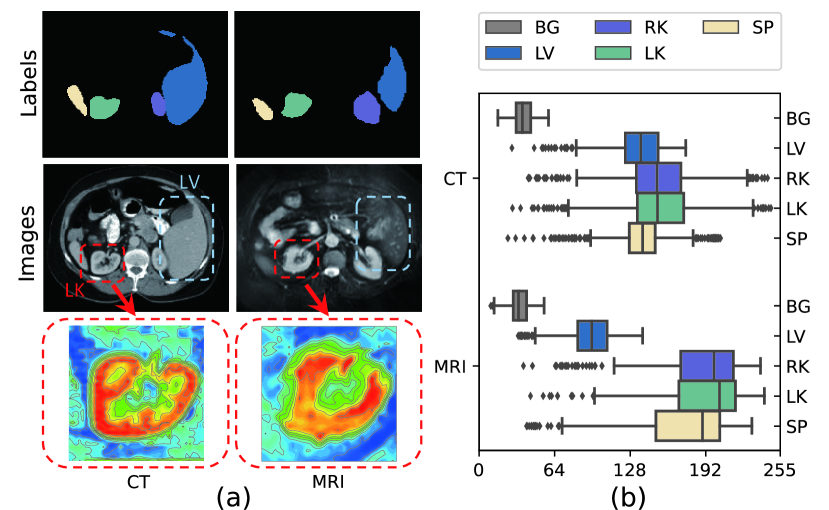
Figure 1: Conceptual overview of our motivation. (a) Different domain images and partial enlarged views (colormap surface). (b) Box-plot of class-specific intensity value distribution across the overall domains of CT&MRI.

Although previous augmentation methods have led to impressive results in generalization tasks, they suffer from the following limitations in medical image segmentation: 1) Global-only augmentation performing transformation on the whole image limits the diversity of augmented images. 2) Random augmentation considers no constraint on the distribution of the augmented samples, which may lead to over-generalization and cause performance degradation. 3) General-task-specific augmentation specially designed for natural image is restricted from medical image tasks, such as weather augmentation (Volk et al. 2019) for automatic driving. These limitations naturally motivate us to think: How to improve augmentation in medical image segmentation? Meanwhile, by looking into medical image segmentation, there are three findings as follows: 1) Class-level representation invariance. Strong similarity exists in the pixel-level representation of the same class between different domains in medical images, as compared with natural images. For an illustrative example in Fig. 1(a), the left kidney (LK) (red dashed square) shows the similar contrast tendency in both CT and MRI domains, i.e. they are relatively bright in the margins and dark in the center. 2) Style mutability. Variance between domains may be reflected in the class-level overall contrast, texture, quality, and clarity. For example, if we compare the liver (LV) (blue dashed square) in Fig. 1(a), it is obvious that this substructure is brighter compared with its surroundings in CT but blends into the background in MRI. This can also be observed through the blue box (LV) in Fig. 1(b), whose mean value is close to other classes in CT but exists a gap in MRI. 3) Segmentation task enjoys inherent advantages owing to pixel-level labels, meaning that the ground truth mask could be used to crop the class-level regions as a unit to perform augmentation. The combination of the class-level augmented samples are much more diverse.

Motivated from these findings, we argue that, in medical scenarios, it is reasonable to hypothesize that the unseen target data can be represented by a linear combination of $C$ (the class number) random variables. Each class-level random variable $x_{U}^{c}$ is sampled from a location-scale distribution. That is to say, $x_{U}=\sum_{c=1}^{C}x_{U}^{c}$, where $x_{U}^{c}=\alpha^{c}x_{S}^{c}+\beta^{c}$. It is noted that a location–scale distribution belongs to a family of probability distributions (e.g. Normal distribution) parameterized by a location parameter and a non-negative scale parameter.

Based on this assumption, we propose a novel augmentation strategy, location-scale augmentation. The augmented data is randomly sampled from the general form $x_{S}^{aug}=\sum_{c=1}^{C}\alpha^{c}x_{S}^{c}+\beta^{c}$, where $\alpha^{c}$ is the scale factor and $\beta^{c}$ is the location factor. With two individual modules: global location-scale augmentation (GLA) and local location-scale augmentation (LLA), this doubling augmentation strategy promotes the diversity of the augmented samples exponentially compared to the previous global-only augmentation. On the empirical front, our method performs constrained B$\acute{\rm e}$zier transformation on both global and local (i.e. class-level) regions. GLA intends to immunize the model against global intensity shift. LLA leverages the mask information to crop the class-level region and perform class-specific transformations, which aims to simulate the class-level distribution shift. Importantly, we make a theoretical analysis in the setting of SDG and prove that the generalization risk can be indeed upper bounded by introducing the location-scale augmentation strategy, thus confirming our hypothesis.

Besides, to address the over-generalization of random augmentation, we further devise a saliency-balancing fusion (SBF) strategy that engages the gradient distribution as an indicator for augmentation magnitude, making our augmentation process informative and oriented. Specifically, we calculate the saliency map and optimize it from noisy to smooth to show the large-gradient area. Such regions in the GLA sample would be preserved, and then fused with LLA sample. As such, the augmented image would be neither too close to the original source distribution nor too far out-of-distribution. Experimental results validate that SBF could achieve a substantially lower source risk compared with the existing random/no fusion mechanism, leading to a tighter generalization bound in our setting.

In summary, we make the following contributions:

1) To the best of our knowledge, we make a first attempt to investigate both global and local augmentation in medical image tasks. We propose a novel augmentation strategy, location-scale augmentation, that engages the inherent class-level information and enjoys a general form of augmentation. Theoretically, we prove that the generalization risk of our augmentation strategy can be upper bounded.

2) We propose a saliency-balancing fusion strategy, providing augmentation with gradient information for proper orientation and intensity. Empirical investigations show saliency-balancing fusion achieves lower source risk, leading to a tighter bound in overall generalization risk.

3) Combining the two strategies, our Saliency-balancing Location-scale Augmentation (SLAug) for SDG achieves superior performance in two segmentation tasks, demonstrating its outstanding generalization capability.

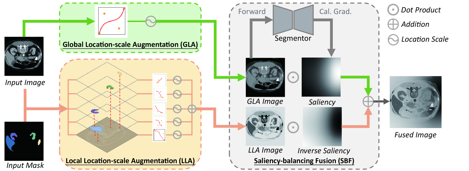
Figure 2: Workflow of the proposed Saliency-balancing Location-scale Augmentation (SLAug).

Related Work

Single-source Domain Generalization

Single-source Domain Generalization (SDG) aims to train a robust and generalizable predictive model against unseen domain shifts with only single source data, which is extremely challenging due to the insufficient diversity in training domain. Several methods (Zhou et al. 2021; Xu et al. 2021; Huang et al. 2020) designed different generation strategies for augmentation in domain generalization tasks. Recently, in medical image fields, Ouyang et al. (2021) used data augmentation to remove the spurious correlations via causal intervention, and Zhou et al. (2022) proposed a dual-normalization based model to tackle the generalization task under cross-modality setting. Different from the previous works, we introduce additive class-level information into augmentation process, significantly boosting the generalization performance.

Mask-based Augmentation

Compared with traditional augmentation (random crop, flipping, etc.), DNN-orientated augmentation is designed from the learning characteristic view of DNNs. Recent efforts (Olsson et al. 2021; Zhang, Zhang, and Xu 2021; Chen et al. 2021) have taken advantages of semantic mask to generate training samples. Olsson et al. (2021) synthesized new samples by cutting half of the predicted classes from one image and then pasting them onto another image. Zhang, Zhang, and Xu (2021) decoupled the image into the background and objects with the mask, and replaced the objects on the inpainted background image. However, the above methods are neither medical-orientated nor designed for domain generalization, making them not suitable in this medical segmentation SDG scenario.

Saliency

Saliency information has been utilized in various fields of machine learning (Wei et al. 2017; Kim, Choo, and Song 2020), which aims to figure out the region of interests in the images. Traditional methods (Wang and Dudek 2014; Hou and Zhang 2007) focused on exploring low-level vision features from images themselves. More recently, deep-learning based methods (Zhao et al. 2015; Simonyan, Vedaldi, and Zisserman 2014) have been proposed for gradient-based saliency detection, which measures the impact of the features of each pixel point in the image on the classification result. In this work, we follow (Simonyan, Vedaldi, and Zisserman 2014) to detect the saliency by computing gradients of a pre-trained model, which does not require modification on the network or additional annotation.

Main Methodology

This section details our proposed Saliency-balancing Location-scale Augmentation (SLAug). As illustrated in Fig. 2, our framework consists of two parts: Location-scale Augmentation and Saliency-balancing Fusion.

Preliminary

In domain generalization tasks, we denote the training samples from the source distribution as $\mathcal{X}_{S}=\{(x_{i,S},m_{i,S})\}_{i=1}^{n_{S}}$ with total classes $C$, where $x_{i,S}$ denotes the $i^{th}$ training sample, $n_{S}$ is the number of training samples, $m_{i,S}$ denotes the corresponding groundtruth mask. Given an unseen distribution $\mathcal{X}_{U}=\{(x_{i,U},m_{i,U})\}_{i=1}^{n_{U}}$, we aim to minimize the error between prediction $\hat{m}_{i,U}$ and groundtruth mask $m_{i,U}$ through a trained segmentor.

Given an image $x$ and its mask $m\in\{1,2,...,C\}^{W\times H}$, $m^{c}$ is defined as the binary mask of class c. $m^{c}_{(w,h)}=1$ means pixel $x_{(w,h)}$ falls in the region of class $c$. The decouple of an image by the semantic class is represented as follows:

$$x^{c}=m^{c}\odot x,\textstyle\sum_{c=1}^{C}x^{c}=x,$$ (1)

where $x^{c}$ are the image regions belong to class $c$, $\odot$ is dot product. Note that since one pixel can correspond to only one class, the mask of one image is constrained as $\textstyle\sum_{c=1}^{C}m^{c}=\textbf{1}$, where 1 presents the all-ones matrix.

Location-scale Augmentation

We consider two types of augmentation, Global Location-scale Augmentation (GLA), which increases the source-like images through global distribution shifting, and Local Location-scale Augmentation (LLA), which conducts class-specific augmentation to explore sufficiently diverse or even extreme appearance of unseen domain.

Different from previous works (Xu et al. 2021; Ouyang et al. 2021), which are based on generic assumptions and utilized random intensity/texture transformations, we leverage the monotonic non-linear transformation for medical images, as the absolute intensity values convey information of the underlying substructures (Buzug 2011; Forbes 2012). Inspired by Model Genesis (Zhou et al. 2019), we choose Cubic B$\acute{\rm e}$zier Curve (Mortenson 1999), a smooth and monotonic function, as our mapping function. Specifically, we constrain our function by the the lowest and highest value of the non-blank image region. That is to say, given an image region with the lowest value $v_{\rm low}$ and highest value $v_{\rm high}$, the constrained B$\acute{\textit{e}}$zier function is given by:

$$B\acute{\textit{e}}zier(t)=\textstyle\sum_{k=0}^{3}(1-t)^{3-k}t^{k}P_{k},t\in[v_{\rm low},v_{\rm high}],$$ (2)

where $t$ is a fractional value along the length of the line. $P_{0}=(v_{\rm low},v_{\rm low})$ and $P_{3}=(v_{\rm high},v_{\rm high})$ are the start and end points to limit the range of value, and $P_{1},P_{2}$ are the control points whose values are randomly generated from [$v_{\rm low}$,$v_{\rm high}$]. The inverse mapping function can be generated by swapping the start point and end point to $P_{0}=(v_{\rm low},v_{\rm high})$ and $P_{3}=(v_{\rm high},v_{\rm low})$. This non-linear transformation function is tagged as $\mathcal{F}_{\rm p}(\cdot)$, where ${\rm p}$ is the probability to perform the inverse mapping.

Before augmentation, $x$ is min-max normalized in the range of [0, 1]. Then, GLA performing global distribution shifting can be described as:

$${\rm GLA}(x)=\alpha\mathcal{F}_{0}(x)+\beta,$$ (3)

where $\alpha\sim\mathcal{TN}(1,\sigma_{1})$, $\beta\sim\mathcal{TN}(0,\sigma_{2})$ are location-scale factors, and $\sigma_{1}$ and $\sigma_{2}$ are standard deviations of the two truncated Gaussian distributions respectively. By using $\mathcal{F}_{0}$, the probability of inverse is zero to ensure the GLA samples have similar appearance with original images. In contrast, LLA takes the individual class-level regions as the processing unit and applies transformation respectively. The augmented regions are then combined linearly. This process can be represented as:

$${\rm LLA}(x,m)=\textstyle\sum_{c=1}^{C}\alpha_{c}\mathcal{F}_{{\rm p}_{c}}(x^{c})+\beta_{c},$$ (4)

where $\alpha_{c}\sim\mathcal{TN}(1,\sigma_{1})$ and $\beta_{c}\sim\mathcal{TN}(0,\sigma_{2})$ are location-scale factors. For all classes, ${\rm p}_{c}=0.5$ is set to apply random inversion, except ${\rm p}_{1}=1$ is set to ensure the LLA augmented images are dissimilar to the GLA samples. It should be noted that we only perform non-linear transformation operations on foreground regions (the non-blank regions in the pictures, representing the human body areas). We visualize the GLA and LLA process in Fig. 3 for better understanding. Empirically, $\sigma_{1}$ is set to be small (e.g. $0.1$ used in the paper), encouraging that the augmented data should stay not further from the source data; $\sigma_{2}$ is set to $0.5$ in this paper, constraining that the “shift” is neither too small nor too big.

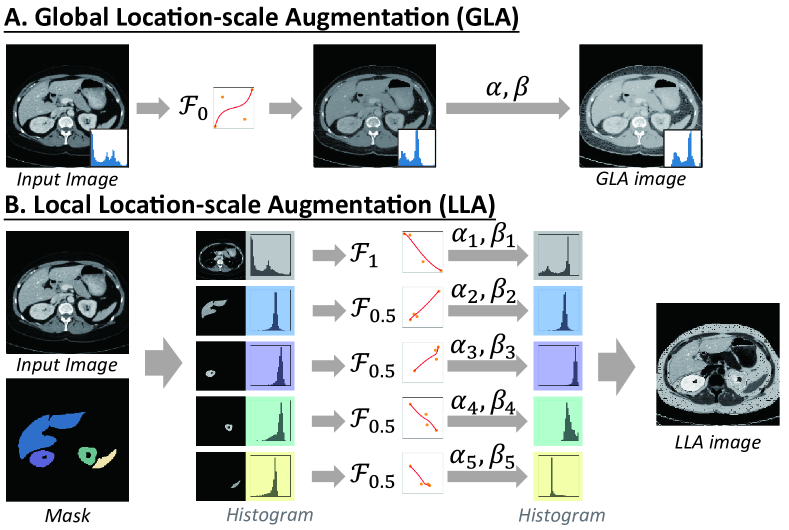
Figure 3: Illustration of proposed global and local location-scale augmentation. $\mathcal{F}_{\rm p}$ denotes the non-linear transformation, while $\alpha$ and $\beta$ are location-scale factors.

Theoretical Evidence

We provide the theoretical evidence to show that our framework can lead to an upper bound of the expected loss on “unseen” but related target domain under our setting.

Assumption 1

The unseen target data can be represented by a linear combination of $C$ (the class number) random variables, each following the location-scale distribution of the source, i.e., $x_{U}=\sum_{c=1}^{C}\alpha^{c}x_{S}^{c}+\beta^{c}$.

Note that Assumption 1 is very mild in the field of medical imaging tasks based on the observation that medical image domain variability is mainly about the overall contrast, texture and clarity at class-level, while other characteristics are comparably more consistent.

Assumption 2

There exists a distribution gap between the generated samples from different augmentations, i.e., $\phi^{aug{{}^{\prime}}}_{S}\neq\phi^{aug{{}^{\prime\prime}}}_{S}$. The $\mathcal{H}$-divergence measured between the two distributions is bounded by $\delta$, which is the largest $\mathcal{H}$-divergence measured between elements of $\sum_{i=1}^{N}\phi^{aug^{i}}_{S}$, i.e., $d_{\mathcal{H}}[{\phi^{aug{{}^{\prime}}}_{S}},{\phi^{aug{{}^{\prime\prime}}}_{S}}]\leq\delta$.

This assumption is satisfied in our setting as the processing steps vary for two augmentation strategy (GLA&LLA), and the variation is bounded by the semantic consistency.

Proposition 1

[Albuquerque et al. (2019)] Define the convex hull $\Lambda_{S}$ as the set of source mixture distributions $\Lambda_{S}=\left\{{\bar{\phi}:\bar{\phi}(\cdot)=\sum_{i=1}^{N_{S}}}\pi_{i}\phi_{S}^{i}(\cdot),\pi_{i}\in\delta_{N_{S}-1}\right\}$, where $\delta_{N_{S}-1}$ is the $N_{S}$-1-th dimensional simplex. The unseen domain composed on a set of unseen distributions $\phi_{U}^{j},j\in[N_{U}]$ is defined as $\phi_{U}$. The labeling rules corresponding to each domain are denoted as $f_{S_{i}}$ and $f_{U_{i}}$. We further introduce $\bar{\phi}_{U}$, the element within $\Lambda_{S}$ which is closest to $\phi_{U}$, i.e., $\bar{\phi}_{U}$ is given by $\mathop{\arg\min}_{\pi_{1},...,\pi_{N_{S}}}d_{\mathcal{H}}[\phi_{U},\sum_{i=1}^{N_{S}}\pi_{i}\phi_{S}^{i}]$. The risk $R_{U}[h],\forall h\in\mathcal{H},$ for any unseen domain $\phi_{U}$ such that $d_{\mathcal{H}}[\bar{\phi}_{U},{\phi}_{U}]=\gamma$ is bounded as:

$$\begin{split}R_{U}[h]&\leq\textstyle\sum_{i=1}^{N_{S}}\pi_{i}R_{S}^{i}[h]+\gamma+{\delta}\\ &+min\left\{\mathbb{E}_{\bar{\phi}_{U}}[|f_{s_{\pi}}-f_{U}|],\mathbb{E}_{{\phi}_{U}}[|f_{U}-f_{s_{\pi}}|]\right\},\end{split}$$ (5)

where $\delta$ is the highest pairwise $\widehat{\mathcal{H}}$-divergence within $\Lambda_{S}$,
$\widehat{\mathcal{H}}=\left\{sign(|h(x)-h^{{}^{\prime}}(x)|-t)|h,h^{{}^{\prime}}(x)\in\mathcal{H},0\leq t\leq 1\right\}$. $f_{S_{\pi}}(x)=\sum_{i=1}^{N_{S}}\pi_{i}f_{S_{i}}(x)$ is the labeling function for any $x\in Supp(\bar{\phi}_{U})$ resulting from combining all $f_{S_{i}}$ with weight $\pi_{i}$, $i\in[N_{S}],\sum_{i=1}^{N_{S}}\pi_{i}=1$, determined by $\bar{\phi}_{U}$.

Theorem 1

Based on Assumption 1 & 2, given data from $N_{S}$ source domains, where the empirical risk of domain i is given as $L(y^{i},y)=\epsilon_{i}\leq\sigma$, the single-source domain generalization risk can be upper bounded by $\sigma+\delta$.

Proof. In our task - single-source domain generalization, the covariate shift assumption (David et al. 2010) holds, the labeling function remains unchanged. When such assumption holds, $f_{S_{\pi}}=f_{{U}}$. The right-most term in Eqn. 5 equals to zero. Based on Assumption 1, the unseen target data can be represented by a linear combination of $C$ random variables sampled from location-scale distribution of the source. Accordingly, data augmentation is implemented with random sampling from the assumed distribution. This can lead to the conclusion that the unseen distribution is actually contained inside the convex hull of the sources, i.e., $\phi_{U}\in\Lambda_{S},\phi_{U}=\bar{\phi}_{U},d_{\mathcal{H}}[\bar{\phi}_{U},{\phi}_{U}]=\gamma=0$. The upper bound would be rewritten as:

$$\begin{split}R_{U}[h]\leq\textstyle\sum_{i=1}^{N_{S}}\pi_{i}R_{S}^{i}[h]+\delta\leq\sigma+\delta.\end{split}$$ (6)

This completes the proof. $\Box$

Notice that the upper bound only depends on the source risk $\sigma$ and the source distribution divergence $\delta$. $\sigma$ is minimized during the training process. As illustrated in Assumption 2, $\delta$ is bounded by the semantic consistency, which means $\delta$ is low in actual experiments. We further validate that the saliency-balancing fusion would lead to a tighter bound compared with no fusion and random fusion through experiments in the following parts.

Algorithm 1 Saliency-balancing Location-scale Augmentation

Require: Training data $(x,m)$, network $f_{\theta}$, loss function $\mathcal{L}$, global location-scale augmentation ${\rm GLA}$, local location-scale augmentation ${\rm LLA}$, common augmentation $F$.

1:  $x^{g}\leftarrow{\rm GLA}(x)$ $\triangleright$ See Eqn.3

2:  $x^{l}\leftarrow{\rm LLA}(x,m)$ $\triangleright$ See Eqn.4

3:  $\tilde{x}^{g},\tilde{x}^{l},\tilde{m}\leftarrow F(x^{g},x^{l},m)$ $\triangleright$ Common augmentation

4:  Calculate gradient Grad = $\nabla_{\tilde{x}^{g}}\mathcal{L}(f_{\theta}(\tilde{x}^{g}),\tilde{m})$

5:  $\textbf{s}\leftarrow\textit{normalize}(\textit{smooth}(\left|\textit{Grad}\right|$)) $\triangleright$ Calculate saliency

6:  $\tilde{x}^{fused}\leftarrow\textbf{s}\odot\tilde{x}^{g}+(1-\textbf{s})\odot\tilde{x}^{l}$

7:  return $\tilde{x}^{fused}$

Saliency-balancing Fusion

We further introduce a gradient distribution harmonizing mechanism named Saliency-balancing Fusion (SBF). The main idea is to preserve the sensitive areas (large-gradient areas) while progressively driving the span of the training data, enabling the augmentation progress to evolve under the guidance of gradient information. Specifically, the saliency map is obtained by taking $l_{2}$ norm of gradient values across input channels and then downsampled to the grid size of $g\times g$ followed by interpolation to the original image size via quadratic B-spline kernels for smoothing.

The whole process can be described as follows: First, we input a GLA augmented image and calculate the saliency map. This step will identify the sensitive areas in source images with slight distribution shifts. Second, we fuse LLA augmented image with GLA augmented image through saliency map, which preserves the large-gradient regions in the GLA augmented image and replace the remaining regions with LLA augmented parts, where drastic changes could be observed in the appearance. Algorithm 1 describes the whole process of our augmentation pipeline, while the above mentioned SBF is detailed in line 4-6. As the fused images contain both parts of the augmented images, SBF encourages the model to behave linearly in-between GLA augmented and LLA augmented examples. We argue that this linear behaviour reduces the amount of undesirable oscillations when predicting out-of-distribution examples compared with directly inputting LLA augmented samples.

Finally, we utilize both GLA augmented images and the saliency-balancing fused images to train the model. The segmentation model $f_{\theta}$ is optimized with the total objective consisting of the cross entropy loss and Dice loss as follows:

$$\mathcal{L}(x,m)=\mathcal{L}_{ce}(x,m)+\mathcal{L}_{dice}(x,m).$$ (7)

Experiments and Results

Datasets and Preprocessing

In our experiments, we evaluate our method on two datasets, cross-modality abdominal dataset (Landman et al. 2015; Kavur et al. 2021) and cross-sequence cardiac dataset (Zhuang et al. 2020). The detailed split of dataset and the preprocessing steps follow the instructions given by  Ouyang et al. (2020), which can be found in the given code. Our proposed approach is used as additional stages followed by common augmentations including Affine, Elastic, Brightness, Contrast, Gamma and Additive Gaussian Noise. All the compared methods (including “ERM” and “Supervised”) conduct the same common augmentation for fair comparison.

Network Architecture and Training Configurations

We utilize U-Net with an EfficientNet-b2 backbone as our segmentation network, same as CSDG (Ouyang et al. 2021). The network is trained from scratch. The grid size $g$ is empirically set to 3 and 18 for abdominal and cardiac datasets respectively. Adam (Kingma and Ba 2014) is used as the optimizer with an initial learning rate of $3\times 10^{-4}$ and weight decay of $3\times 10^{-5}$. The learning rate remains unchanged for the first 50 epochs and linearly decays to zero over the next 1,950 epochs. For all experiments, batch size is set to 32 and the methods are evaluated at the 2,000^th epoch. We implemented our framework on a workstation equipped with one NVIDIA GeForce RTX 3090 GPU (24G memory).

Method	Abdominal CT-MRI					Cardiac bSSFP-LGE
	Liver	R-Kidney	L-Kidney	Spleen	Average	LVC	MYO	RVC	Average
Supervised	91.30	92.43	89.86	89.83	90.85	92.04	83.11	89.30	88.15
ERM	78.03	78.11	78.45	74.65	77.31	86.06	66.98	74.94	75.99
Cutout	79.80	82.32	82.14	76.24	80.12	88.35	69.06	79.19	78.87
RSC	76.40	75.79	76.60	67.56	74.09	87.06	69.77	75.69	77.51
MixStyle	77.63	78.41	78.03	77.12	77.80	85.78	64.23	75.61	75.21
AdvBias	78.54	81.70	80.69	79.73	80.17	88.23	70.29	80.32	79.62
RandConv	73.63	79.69	85.89	83.43	80.66	89.88	75.60	85.70	83.73
CSDG	86.62	87.48	86.88	84.27	86.31	90.35	77.82	86.87	85.01
SLAug (ours)	90.08	89.23	87.54	87.67	88.63	91.53	80.65	87.90	86.69
Method	Abdominal MRI-CT					Cardiac LGE-bSSFP
	Liver	R-Kidney	L-Kidney	Spleen	Average	LVC	MYO	RVC	Average
Supervised	98.87	92.11	91.75	88.55	89.74	91.16	82.93	90.39	88.16
ERM	87.90	40.44	65.17	55.90	62.35	90.16	78.59	87.04	85.26
Cutout	86.99	63.66	73.74	57.60	70.50	90.88	79.14	87.74	85.92
RSC	88.10	46.60	75.94	53.61	66.07	90.21	78.63	87.96	85.60
MixStyle	86.66	48.26	65.20	55.68	63.95	91.22	79.64	88.16	86.34
AdvBias	87.63	52.48	68.28	50.95	64.84	91.20	79.50	88.10	86.27
RandConv	84.14	76.81	77.99	67.32	76.56	91.98	80.92	88.83	87.24
CSDG	85.62	80.02	80.42	75.56	80.40	91.37	80.43	89.16	86.99
SLAug (ours)	89.26	80.98	82.05	79.93	83.05	91.92	81.49	89.61	87.67

Table 1: Performance comparison of different methods. Dice score (%) is utilized as the evaluation metrics.

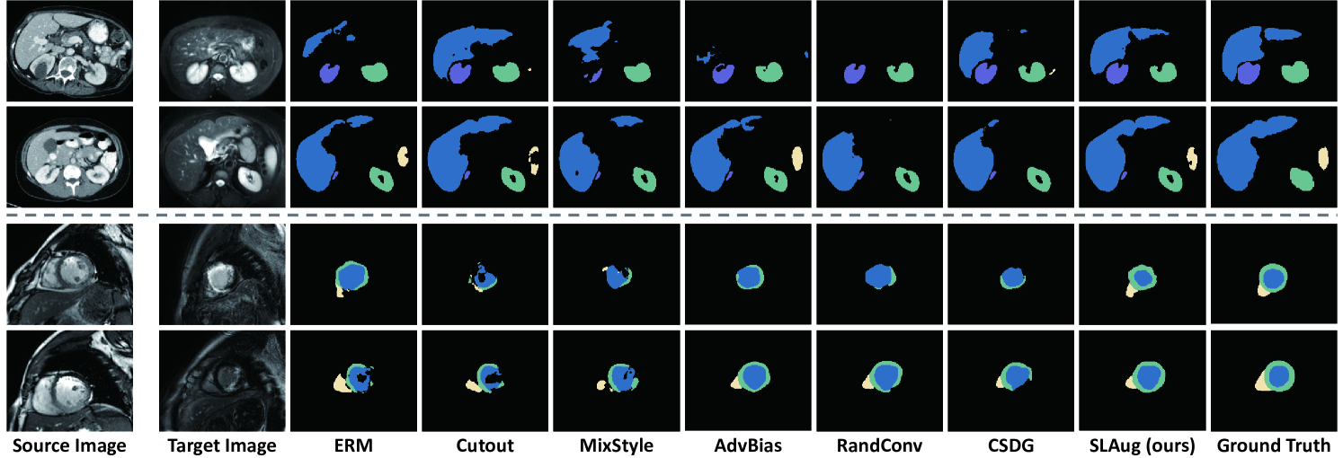
Figure 4: Qualitative comparison for Abdominal CT-MRI (top two rows) and Cardiac bSSFP-LGE (bottom two rows).

Results and Comparative Analysis

To quantify the instance segmentation performance of each method, we engage the Dice score (Milletari, Navab, and Ahmadi 2016) as the evaluation metric for measuring the overlap between the prediction and ground truth.

We compare our proposed method with the baseline empirical risk minimization (ERM) and the state-or-the-art methods (e.g. Cutout, RSC, MixStyle, AdvBias, RandConv, and CSGD) in the abdominal and cardiac segmentation. Cutout (DeVries and Taylor 2017) improves the model robustness and overall performance by randomly masking out square regions. RSC (Huang et al. 2020) forces the model to learn more general features by iteratively discarding the dominant features. MixStyle (Zhou et al. 2021) generates novel images by mixing styles of training instances at the bottom layers of the network. AdvBias (Chen et al. 2020) generates plausible and realistic signal corruptions, which models the intensity inhomogeneities in an adversarial way. To randomize the image intensity and texture, RandConv (Xu et al. 2021) employs transformation via randomly initializing the weight of the first convolution layer. CSDG (Ouyang et al. 2021) further improves RandConv by extending the random module to a shallow network, and then mixes two augmented images through the pseudo correlations map to alleviate the spurious spatial correlations.

The quantitative performance of different methods is presented in Tab. 1. Overall, our method significantly outperforms the previous methods by a large margin. To be specific, we improve the performance of SDG by 47.77% compared with the latest work CSDG in the four experiments on average, greatly narrowing the gap between single-source domain generalization and the upper bound. In abdominal cross-modality experiments, our method achieves the highest average Dice score of 88.63 and 83.05 in both directions. Compared with the most competitive method CSDG which engages a random texture augmentation, SLAug leads to an average improvement of 2.49 Dice score, demonstrating its superiority in cross-modality scenarios. In cardiac cross-sequence experiments, we observe the unequal difficulty between the generalization direction of “bSSFP to LGE” and “LGE to bSSFP”. Our method performs steadily in either small or large domain gap situation, leading to an increase of 1.68 and 0.43 compared with the best performance in previous methods. This indicates that SLAug has better domain generalization capability in various medical image distributions with diverse domain gaps. The visualization of different methods is presented in Fig. 4. We also show the source and target domain images in the first two columns, illustrating the appearance shift between domains. It is clearly observed that our method generates few misclassified predictions in the unseen target domain.

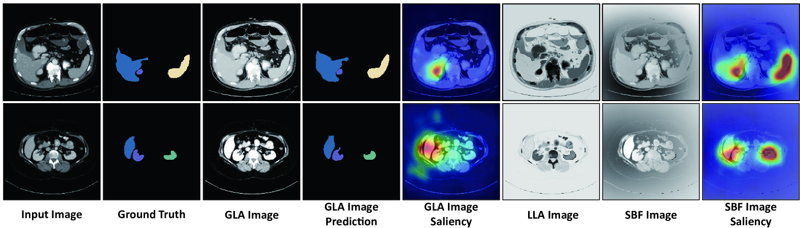
Figure 5: Visualization of the saliency map from intermediate results of SLAug.

Analytical Experiments

Ablation Study.

We conduct ablation studies on the three main components in SLAug to better demonstrate our contribution, i.e., the Global Location-scale Augmentation (GLA), the Local Location-scale Augmentation (LLA), and Saliency-balancing Fusion (SBF). Tab. 2 presents the performance of different variants of SLAug in two tasks - abdominal cross-modality and cardiac cross-sequence segmentation. Comparing Variant 1, 2 with ERM, we can observe that solely utilizing GLA or LLA could steadily improve the overall performance. However, GLA and LLA can only boost the performance in one of the two tasks, indicating either GLA or LLA is not applicable for both types of tasks. Variant 2 indicates that utilizing mask-based augmentation could lead to a gain in performance, but once GLA is combined (e.g. Variant 3), the obtained results could even outperform most SOTA methods. Then, we add SBF based on Variant 1,2 and 3. For Variant 4 and 5, we augment the images with the same augmentation twice, and use one of them to generate the saliency map to fuse the two images. The performance improvement of Variant 4 over Variant 1 implies that the saliency information from GLA augmented images plays a vital role in our method, as it can indicate the data distribution near the decision boundary of the source domain, thus providing guidance for distribution enlargement. Also, the marginal performance degradation in Variant 5 over Variant 2 also supports this claim. We assume that the saliency information derived from LLA augmented samples is inaccurate since LLA samples vary a lot from the original source samples, which leads to the decrease of the overall performance. Finally, SLAug performs the best, showing that the three components promote mutually and are all indispensable for the superior domain generalization.

Methods	GLA	LLA	SBF	Abd.	Card.	Avg.
ERM	-	-	-	77.31	75.99	76.65
Variant 1	✓	-	-	80.28	74.21	77.25
Variant 2	-	✓	-	75.43	85.12	80.28
Variant 3	✓	✓	-	85.48	85.55	85.52
Variant 4	✓	-	✓	83.57	82.39	82.98
Variant 5	-	✓	✓	75.42	85.00	80.21
SLAug	✓	✓	✓	88.63	86.69	87.66

Table 2: Ablation study of SLAug on the direction of abdominal CT-MRI (Abd.) and cardiac bSSFP-LGE (Card.).

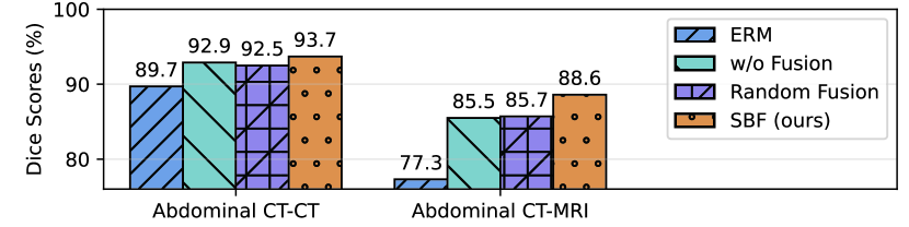
Figure 6: Comparisons of ERM and different fusion methods on location-scale augmented images in Abdominal task.

Effectiveness of Saliency-balancing Fusion.

To investigate the benefits of the guidance from saliency for image fusion, we replace the saliency map with a randomly initialized map. As shown in Fig. 6, random fusion slightly improves the performance by 0.2 Dice score against without (w/o) fusion in cross-domain (CT-MRI) scenarios. This indicates the mixture of two augmented images could improve the generalization performance, which, may benefit from the enrichment of the augmented samples. However, this result is much lower than SBF by 2.9 in Dice score, as we consider SBF is much more informative and explainable compared with random fusion. Moreover, we compare the source test set results as a metric for the preserving capability of source-domain knowledge, as shown in Fig. 6 by the CT-CT bars. A reduction of 0.4 Dice score can be observed by using random fusion against directly inputting the two augmented images into training (w/o fusion). In contrast, our SBF promotes the source performance by 0.8 in comparison with no fusion, and 4.0 compared with empirical risk minimization (ERM). This result corresponds to the first term of the upper bound in Eqn. 6, showing that SBF could achieve a tighter generalization bound by lowering the source risk.

Besides demonstrating the effectiveness of SBF by numerical values, we provide the visualization of the saliency maps and the predictions of the GLA augmented image, serving as the indicator for its interpretability and informativeness in Fig. 5. From these pictures, we can infer that 1) saliency map can provide accurate feedback on the sensitive regions in GLA step. If we focus on the large-gradient areas in saliency map, we would find that these areas are misclassified in GLA prediction. 2) LLA enforces larger augmentation intensity on the given samples. Saliency maps in the last column show more salient areas in comparison to the GLA images saliency maps. 3) SBF could effectively combine the sensitive areas in GLA images while introduce larger augmentation magnitude in the remaining areas. The fused images can locate the vital areas, which is beneficial for gradient harmonizing, so as to boost the generalization capability of the training model.

Conclusion

In this paper, we propose a novel augmentation strategy to better solve the single-source domain generalization problems in medical image segmentation. By jointly integrate the location-scale augmentation and saliency-balancing fusion, this plug-and-play module shows superior performance on two challenging tasks. Moreover, we provide the theoretical evidence and visualization examples for better explanation, aiming to facilitate more principled techniques for robust learning in medical fields.

Appendix A Appendix

Additive Experimental Details

In our experiments, we evaluate our method on two datasets. The first cross-modality abdominal dataset includes 30 volumes of CT data (Landman et al. 2015), and 20 volumes of T2-SPIR MRI data (Kavur et al. 2021). We conduct a 70%-10%-20% data split for training, validation and testing set on source domain. All the target domain images are used to evaluate the domain generalization performance, same in (liu2020shape). The second dataset is cross-sequence cardiac segmentation dataset (Zhuang et al. 2020), which consists of 45 balanced steady-state free precession (bSSFP) and 45 late gadolinium enhanced (LGE) MRI volumes. Data split in direction “bSFFP to LGE” is the same as in the challenge (Zhuang et al. 2020), and the training and test sets are interchanged in the opposite direction.

The preprocessing steps follow the instructions given by  Ouyang et al. (2020). All the 3D volumes are spatial normalized and reformatted into 2D slices, and then cropped/resized to $192\times 192$ on XY-plane. For the abdominal CT dataset, a window of [-275, 125] (Ouyang et al. 2020) is applied on Hounsfield values. For the MRI datasets, the top 0.5% intensity histogram are clipped. Our proposed approach is used as additional stages followed by common augmentations including Affine, Elastic, Brightness, Contrast, Gamma and Additive Gaussian Noise. All the compared methods (including “ERM” and “Supervised”) conduct the same common augmentation for fair comparison. The details of common augmentations are included in Tab. S3, which are applied to all methods by default. The parameters setting is the same with Ouyang et al. (2021).

During training, all the augmentations applied to GLA and LLA image for one slice are in the same random states. The same geometric transformations such as Affine and Elastic transformations ensure the two augmented images can be fused without spatial difference. The same intensity augmentations including Brightness, Contrast and Gamma augmentations can maintain the appearance difference caused by location-scale augmentations.

Augmentations	Parameters
Affine Transformation	Rotate: 20 Shift: 15 Shear: 20 Scale: [0.5, 1.5]
Elastic Transformation	Alpha: 20 Sigma: 5
Brightness	Brightness: [-10,10]
Contrast	Contrast: [0.6,1.5]
Gamma	Gamma: [0.2, 1.8]
Additive Gaussian Noise	Noise std: 0.15

Table S3: Parameters of common augmentations used in all experiments by default.

Hyper-parameter Analysis

We give an experimental analysis of the grid size $g$ as shown in Fig. S7, which is utilized to smooth the gradient map. As can be observed in the figure, the performance remains steady with the change of grid size. Note that grid size $=1$ means the saliency map equals to 1 everywhere, so only GLA images contribute to the final fused image.

As the grid size affects the smoothness of the fine-grained fusion map, we conjecture that this parameter is related to the size and spatial distribution of each class. Different from segmenting separate organs in abdominal segmentation, the substructures in cardiac segmentation are more closer to each other. Therefore, a less smooth fusion map is expected in cardiac segmentation to ensure a higher resolution fusion map to distinguish each components inside the heart. Generally, the grid size is suggested to set large if the classes are close to each other.

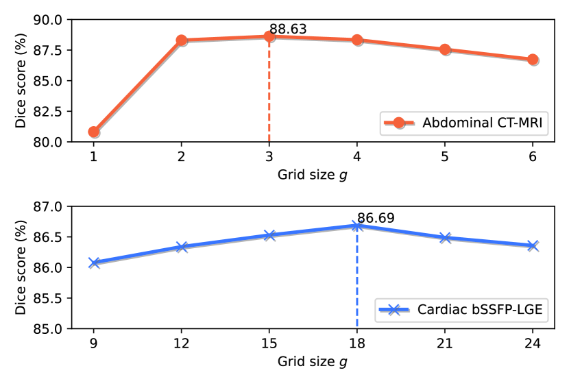
Figure S7: Influence of grid size $g$ on two experiments.

More Visualization

To better illustrate the Bezier Curve transformation, we demonstrate some cases in Fig. S8. The 1st column is the raw images which have been normalized in $[0,1]$. The start point $P_{0}=(0,0)$ and end point $P_{3}=(1,1)$ is set for simplicity, except $P_{0}=(0,1)$, $P_{3}=(1,0)$ is set at 7th columns for intensity inversion.

Meanwhile, we give more visualization of comparative results in Fig. S9, consisting of Abdominal MRI-CT and Cardiac LGE-bSSFP segmentation.

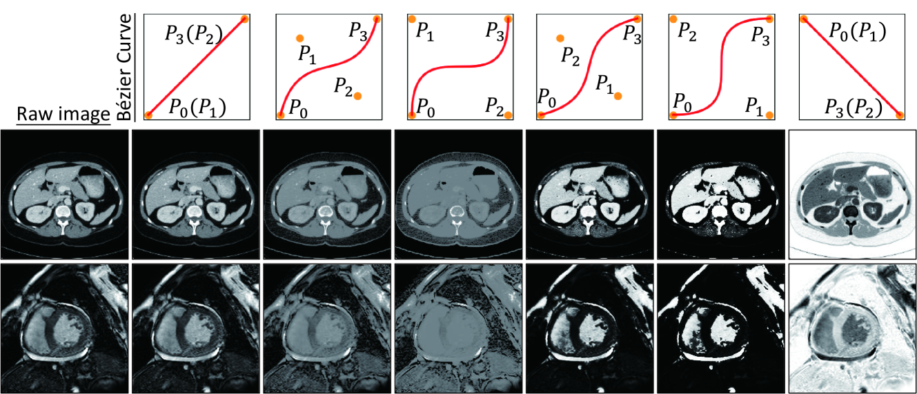
Figure S8: Demonstration of bezier curve and augmented images.

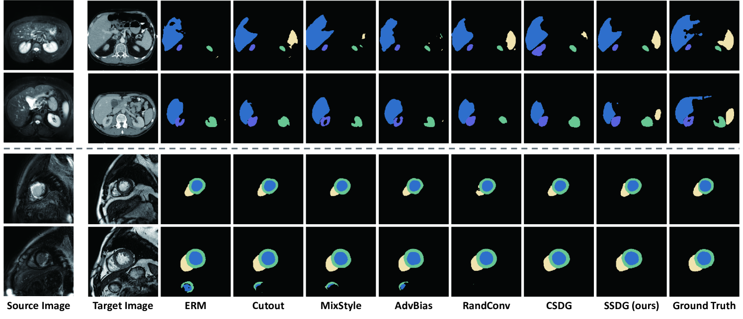
Figure S9: Additive quantitative comparison for Abdominal MRI-CT (top two rows) and Cardiac LGE-bSSFP (bottom two rows).From left to right are the source domain images (1st column), the target domain images (2rd column), results of other comparative methods (3nd-8th columns), results of our proposed SLAug (9th column) and ground truth (last column).

References

- Albuquerque et al. (2019) Albuquerque, I.; Monteiro, J.; Darvishi, M.; Falk, T. H.; and Mitliagkas, I. 2019. Generalizing to unseen domains via distribution matching. arXiv:1911.00804.
- Buzug (2011) Buzug, T. M. 2011. Computed tomography. In Springer handbook of medical technology, 311–342. Springer.
- Chen et al. (2019) Chen, C.; Dou, Q.; Chen, H.; Qin, J.; and Heng, P.-A. 2019. Synergistic image and feature adaptation: Towards cross-modality domain adaptation for medical image segmentation. In AAAI Conference on Artificial Intelligence, volume 33, 865–872.
- Chen et al. (2020) Chen, C.; Qin, C.; Qiu, H.; Ouyang, C.; Wang, S.; Chen, L.; Tarroni, G.; Bai, W.; and Rueckert, D. 2020. Realistic adversarial data augmentation for MR image segmentation. In International Conference on Medical Image Computing and Computer-Assisted Intervention, 667–677. Springer.
- Chen et al. (2021) Chen, Y.; Ouyang, X.; Zhu, K.; and Agam, G. 2021. Mask-based data augmentation for semi-supervised semantic segmentation. arXiv:2101.10156.
- David et al. (2010) David, S. B.; Lu, T.; Luu, T.; and Pál, D. 2010. Impossibility theorems for domain adaptation. In Proceedings of the Thirteenth International Conference on Artificial Intelligence and Statistics, volume 9, 129–136.
- DeVries and Taylor (2017) DeVries, T.; and Taylor, G. W. 2017. Improved regularization of convolutional neural networks with cutout. arXiv:1708.04552.
- Forbes (2012) Forbes, G. B. 2012. Human body composition: growth, aging, nutrition, and activity. Springer Science & Business Media.
- Hou and Zhang (2007) Hou, X.; and Zhang, L. 2007. Saliency detection: A spectral residual approach. In 2007 IEEE Conference on computer vision and pattern recognition, 1–8. Ieee.
- Huang et al. (2020) Huang, Z.; Wang, H.; Xing, E. P.; and Huang, D. 2020. Self-challenging improves cross-domain generalization. In European Conference on Computer Vision, 124–140. Springer.
- Kavur et al. (2021) Kavur, A. E.; Gezer, N. S.; Barış, M.; Aslan, S.; Conze, P.-H.; Groza, V.; Pham, D. D.; Chatterjee, S.; Ernst, P.; Özkan, S.; et al. 2021. CHAOS challenge-combined (CT-MR) healthy abdominal organ segmentation. Medical Image Analysis, 69: 101950.
- Kim, Choo, and Song (2020) Kim, J.-H.; Choo, W.; and Song, H. O. 2020. Puzzle mix: Exploiting saliency and local statistics for optimal mixup. In International Conference on Machine Learning, 5275–5285. PMLR.
- Kingma and Ba (2014) Kingma, D. P.; and Ba, J. 2014. Adam: A Method for Stochastic Optimization. arXiv:1412.6980.
- Landman et al. (2015) Landman, B.; Xu, Z.; Igelsias, J.; Styner, M.; Langerak, T.; and Klein, A. 2015. Miccai multi-atlas labeling beyond the cranial vault-workshop and challenge. In Proc. MICCAI Multi-Atlas Labeling Beyond Cranial Vault—Workshop Challenge, volume 5, 12.
- Milletari, Navab, and Ahmadi (2016) Milletari, F.; Navab, N.; and Ahmadi, S.-A. 2016. V-net: Fully convolutional neural networks for volumetric medical image segmentation. In International Conference on 3D Vision, 565–571. IEEE.
- Mortenson (1999) Mortenson, M. E. 1999. Mathematics for computer graphics applications. Industrial Press Inc.
- Olsson et al. (2021) Olsson, V.; Tranheden, W.; Pinto, J.; and Svensson, L. 2021. Classmix: Segmentation-based data augmentation for semi-supervised learning. In Proceedings of the IEEE/CVF Winter Conference on Applications of Computer Vision, 1369–1378.
- Ouyang et al. (2020) Ouyang, C.; Biffi, C.; Chen, C.; Kart, T.; Qiu, H.; and Rueckert, D. 2020. Self-supervision with superpixels: Training few-shot medical image segmentation without annotation. In European Conference on Computer Vision, 762–780. Springer.
- Ouyang et al. (2021) Ouyang, C.; Chen, C.; Li, S.; Li, Z.; Qin, C.; Bai, W.; and Rueckert, D. 2021. Causality-inspired Single-source Domain Generalization for Medical Image Segmentation. arXiv:2111.12525.
- Simonyan, Vedaldi, and Zisserman (2014) Simonyan, K.; Vedaldi, A.; and Zisserman, A. 2014. Deep Inside Convolutional Networks: Visualising Image Classification Models and Saliency Maps. In 2nd International Conference on Learning Representations, ICLR 2014, Banff, AB, Canada, April 14-16, 2014, Workshop Track Proceedings.
- Valanarasu et al. (2021) Valanarasu, J. M. J.; Oza, P.; Hacihaliloglu, I.; and Patel, V. M. 2021. Medical Transformer: Gated Axial-Attention for Medical Image Segmentation. In de Bruijne, M.; Cattin, P. C.; Cotin, S.; Padoy, N.; Speidel, S.; Zheng, Y.; and Essert, C., eds., Medical Image Computing and Computer Assisted Intervention, volume 12901, 36–46.
- Volk et al. (2019) Volk, G.; Müller, S.; Von Bernuth, A.; Hospach, D.; and Bringmann, O. 2019. Towards robust CNN-based object detection through augmentation with synthetic rain variations. In 2019 IEEE Intelligent Transportation Systems Conference, 285–292.
- Wang and Dudek (2014) Wang, B.; and Dudek, P. 2014. A fast self-tuning background subtraction algorithm. In Proceedings of the IEEE Conference on Computer Vision and Pattern Recognition Workshops, 395–398.
- Wang et al. (2020) Wang, S.; Yu, L.; Li, K.; Yang, X.; Fu, C.-W.; and Heng, P.-A. 2020. Dofe: Domain-oriented feature embedding for generalizable fundus image segmentation on unseen datasets. IEEE Transactions on Medical Imaging, 39(12): 4237–4248.
- Wei et al. (2017) Wei, Y.; Feng, J.; Liang, X.; Cheng, M.-M.; Zhao, Y.; and Yan, S. 2017. Object region mining with adversarial erasing: A simple classification to semantic segmentation approach. In Proceedings of the IEEE conference on computer vision and pattern recognition, 1568–1576.
- Xu et al. (2021) Xu, Z.; Liu, D.; Yang, J.; Raffel, C.; and Niethammer, M. 2021. Robust and Generalizable Visual Representation Learning via Random Convolutions. In International Conference on Learning Representations.
- Yao et al. (2022) Yao, K.; Su, Z.; Huang, K.; Yang, X.; Sun, J.; Hussain, A.; and Coenen, F. 2022. A novel 3D unsupervised domain adaptation framework for cross-modality medical image segmentation. IEEE Journal of Biomedical and Health Informatics.
- Zhang, Zhang, and Xu (2021) Zhang, J.; Zhang, Y.; and Xu, X. 2021. Objectaug: object-level data augmentation for semantic image segmentation. In 2021 International Joint Conference on Neural Networks (IJCNN), 1–8. IEEE.
- Zhao et al. (2015) Zhao, R.; Ouyang, W.; Li, H.; and Wang, X. 2015. Saliency detection by multi-context deep learning. In Proceedings of the IEEE conference on computer vision and pattern recognition, 1265–1274.
- Zhou et al. (2021) Zhou, K.; Yang, Y.; Qiao, Y.; and Xiang, T. 2021. Domain Generalization with MixStyle. In International Conference on Learning Representations.
- Zhou et al. (2022) Zhou, Z.; Qi, L.; Yang, X.; Ni, D.; and Shi, Y. 2022. Generalizable Cross-modality Medical Image Segmentation via Style Augmentation and Dual Normalization. In Proceedings of the IEEE/CVF Conference on Computer Vision and Pattern Recognition, 20856–20865.
- Zhou et al. (2019) Zhou, Z.; Sodha, V.; Rahman Siddiquee, M. M.; Feng, R.; Tajbakhsh, N.; Gotway, M. B.; and Liang, J. 2019. Models genesis: Generic autodidactic models for 3d medical image analysis. In International conference on medical image computing and computer-assisted intervention, 384–393. Springer.
- Zhuang et al. (2020) Zhuang, X.; Xu, J.; Luo, X.; Chen, C.; Ouyang, C.; Rueckert, D.; Campello, V. M.; Lekadir, K.; Vesal, S.; RaviKumar, N.; et al. 2020. Cardiac segmentation on late gadolinium enhancement MRI: a benchmark study from multi-sequence cardiac MR segmentation challenge. arXiv:2006.12434.